a hybrid cultural-harmony algorithm for multi-objective...

Scientia Iranica E (2015) 22(3), 1227{1241

Sharif University of TechnologyScientia Iranica

Transactions E: Industrial Engineeringwww.scientiairanica.com

A hybrid cultural-harmony algorithm formulti-objective supply chain coordination

S. Alaei and F. Khoshalhan�

Department of Industrial Engineering, KNT University of Technology, Tehran, Iran.

Received 2 October 2013; received in revised form 20 April 14; accepted 17 November 2014

KEYWORDSSupply chaincoordination;Meta-heuristics;Taguchi method;Supplier selection;Cultural algorithm;Harmony search.

Abstract. We investigate a one-buyer, multi-vendor, coordination model with a vendorselection problem in a centralized supply chain. In the proposed model, the buyer selectsone or more vendor and orders an appropriate quantity. The quantity discount mechanismis used by all vendors with the aim of coordinating the supply chain. We formulatethe problem as a multi-objective mixed integer nonlinear mathematical model. Usingthe Global Criterion method, the proposed model is transformed into a single objectiveoptimization problem. Since the problem is NP-hard, we propose four meta-heuristicalgorithms: Particle Swarm Optimization (PSO), Scatter Search (SS), population basedHarmony Search (HS-pop) and Harmony Search based Cultural Algorithm (HS-CA). TheTaguchi robust tuning method is applied in order to estimate the optimum values ofparameters. Then, the solution quality and computational time of the algorithms arecompared.

c 2015 Sharif University of Technology. All rights reserved.

1. Introduction

Coordination between all entities in a supply chainand global planning is necessary to achieve e�ectiveSupply Chain Management (SCM) [1]. In the lackof cooperation, supply chain members are willing tooptimize their own objectives independently, whichmay lead to channel ine�ciency. Designing mecha-nisms for coordinating and aligning decisions betweenentities is of great importance in supply chain man-agement. Several coordination mechanisms have beenapplied in the literature, such as the wholesale pricecontract [2], two-part tari� [3], buyback [4], revenuesharing [5], quantity exibility [6], back-up [7], salesrebate [8], quantity discount [9], timing discount [10],and the revenue sharing reservation contract withpenalty [11].

*. Corresponding author. Tel.: +98 21 84063347;E-mail addresses: [email protected] (S. Alaei);[email protected] (F. Khoshalhan)

Supplier (vendor) selection is a strategic decisionwhen a buyer tries to establish a win-win businessrelationship with its supplier. It is one of the mostcritical components of the purchasing function of a�rm [12]. Vendor selection and order allocation aretwo main features to be considered in supply chainmanagement.

Suppose a typical channel with a single buyerand multiple vendors. The buyer faces a four-objective constrained problem, i.e. selecting one ormore vendor(s) in order to allocate his order quantityfor satisfying market demand. All the vendors o�erquantity discounts to motivate buyers to order morequantities. The coordination of this supply chainis studied in context to examine the performance ofdi�erent metaheuristic algorithms.

Some models have been developed to investigatethe coordination problem and the vendor selectionproblem. However, little attention has been paidto developing e�cient algorithms in this area. Inthis paper, we consider four metaheuristic algorithms.

1228 S. Alaei and F. Khoshalhan/Scientia Iranica, Transactions E: Industrial Engineering 22 (2015) 1227{1241

The population based Harmony Search (HS-pop) andHarmony Search based Cultural Algorithm (HS-CA)are two hybrid algorithms that are proposed for com-parison with already developed algorithms in this area(i.e. Particle Swarm Optimization (PSO) and ScatterSearch (SS)).

The main contributions of the article are:

1. The Harmony Search (HS) algorithm and the Cul-tural Algorithm are incorporated (CA). We assumethat the situational knowledge component of theCA belief space acts as a harmony memory. More-over, o�spring are generated using HS operatorsand CA belief space.

2. In the HS-pop algorithm, the reproduction processand updating the harmony memory are modi�edcompared to the traditional HS algorithm.

The objectives of the research are:

1. To investigate multi-objective coordination of asupply chain using a quantity discount contract;

2. To compare the performance of two hybrid algo-rithms with other metaheuristic algorithms. Usingnumerical study, we perform analyses over solutionqualities and computational e�ort.

We apply the Taguchi robust tuning method in orderto estimate the optimum values of parameters. TheRelative Percentage Deviation (RPD) is used to assessthe quality of solutions. Moreover, in order to evaluatethe computational time of the proposed algorithms, thetime to reach a solution with r% error (i.e. 1% or 3%) iscomputed. We investigate the Convergence Index (CI)of the proposed algorithms, as the number of successfulruns with which the algorithm reaches a solution, withr% error, over the total number of runs.

The remainder of the paper is organized as fol-lows: Section 2 brie y reviews the related literature.Section 3 describes the problem and notation. Section 4presents the solution procedure and four metaheuristicalgorithms. In Section 5, the Taguchi method is usedfor tuning parameters of the algorithms. Section 6provides an illustrative example. The proposed algo-rithms are evaluated using the numerical example inSection 7. Finally, Section 8 summarizes and concludesthe paper.

2. Literature review

We provide a brief review of supply chain coordi-nation and supplier selection models that have beenstudied in recent years. Rosenthal et al. [13] studieda supplier selection problem with multiple products,where suppliers o�er discounts when a \bundle" ofproducts is bought. Sarkis and Semple [14] discussed asingle period supplier selection problem with business

volume discounts, wherein the total purchasing costshould be optimized without taking inventory-relatedcosts into account. Goossens et al. [15] studied amulti items supplier selection, wherein the supplierso�er an all-unit quantity discount and try to mini-mize the total cost of purchasing. Ghodsypour andO'Brien [16] developed an integrated AHP and linearprogramming model, in which both qualitative andquantitative factors are considered in the process ofsupplier selection and order allocation. Amid et al. [17]proposed a weighted additive fuzzy multi-objectivemodel for the supplier selection problem under all-unitprice discounts.

Jayaraman et al. [18] developed a Mixed Integerlinear Programming (MIP) model, wherein qualityproduction capacity, lead-time, and storage capacitylimits are considered. Another MIP model for thesupplier selection is proposed by Cakravastia et al. [19]where the objective is to minimize the level of customerdissatisfaction, which was evaluated by price and leadtime. Dahel [20] developed a Multi-Objective MixedInteger Programming (MO-MIP) model with multipleproducts and discounts on total business volume. Xiaand Wu [21] presented a MO-MIP approach under atotal business volume discount, and used an integratedAHP method and multi-objective programming toinvestigate the problem. Ebrahim et al. [22] developeda MO-MIP model with di�erent types of discountand proposed a scatter search algorithm to solve theproblem.

Herer et al. [23] were the �rst to propose asupplier selection problem together with coordinationmodels. The limited annual production rate andinventory holding costs are taken into account in theirmodel. Kim and Goyal [24] investigated two di�erentshipment policies from the suppliers to the buyer inwhich suppliers deliver their production lots eithersimultaneously or successively. Kamali et al. [25]developed a multi-objective mixed integer nonlinearprogramming model to coordinate the system of asingle-buyer- multi-vendors, under an all-unit quantitydiscount. They proposed Particle Swarm Optimizationand Scatter Search for solving the problem. Gheidar-Kjeljani [26] proposed a nonlinear mathematical modelwhich is a combination of a supplier selection modeland a coordination model in a centralized supply chain.In their model, the buyer ordered quantities are splitinto small lot sizes and are delivered to the buyer overmultiple periods.

3. Problem description

A typical channel with one buyer and multiple vendorsis considered. The buyer selects one or more vendorsin order to allocate his order quantity for satisfyingmarket demand without any type of shortage. All the

S. Alaei and F. Khoshalhan/Scientia Iranica, Transactions E: Industrial Engineering 22 (2015) 1227{1241 1229

Figure 1. Supply chain members.

vendors o�er quantity discounts to motivate buyers toorder more quantities. A schematic view of the supplychain is illustrated in Figure 1. Selecting suitablevendors for supplying the products is an important partof the operation.

The buyer has to choose one or more vendor(s)and purchase an optimal level of single product fromeach vendor based on various objectives. The buyerhas a dilemma, due to discount contracts o�ered bythe vendors, which depend on the volume of the orderquantity. The objectives considered in this paperfor choosing potential vendors are similar to those ofKamali et al. [25]; they are:

a) Minimizing the whole supply chain annual costs;

b) Minimizing the total defective items ordered by thebuyer;

c) Minimizing the total late delivered items;

d) Maximizing the total annual purchasing value.

Suppose that there are n vendors in the supply chain.Each of them (i.e., vendor i) o�ers an all-unit quantitydiscount with Ki price level, each level (i.e. level k) ischaracterized by an interval, [ui;k�1; uik), and the priceof cik is associated with this interval. For example, foreach vendor, i, we have ui1 < ui2 < � � � < ui;Ki andci1 > ci2 > � � � > ci;Ki . Also, assume that vendor orderquantities are dispatched to the buyer in a sequentialorder. In other words, after consuming the productsof one vendor, the products of another vendor can beentered.

Parameters used in the problem:D Buyer annual �xed market demand

rate;Si Fixed setup cost associated with

vendor i;Ai Buyer �xed ordering cost for vendor i;

hi Vendor i's inventory holding cost perunit, per unit time;

h Retailer's �xed inventory holding costper unit, per unit time (independent ofpurchasing cost);

Ti Consumption time of an order quantityfrom vendor i;

T Cycle time of the retailer;zi Unit variable cost of vendor i;Pi Production rate associated with vendor

i;bik Quantity at which the kth price break

occurs by vendor i;Ri Reliability of time of delivery of

products for vendor i;di Defective rate that vendor i maintains;wi Total weight assigned to vendor i.

Decision variables used in the model:qik Number of units supplied by vendor i

at price level k in a cycle;yik Binary variable denoting whether order

quantity is chosen from k's price levelor not;

Qi Order quantity supplied by vendor i ina cycle, i.e. Qi =

PKik=1 qik;

Q Total order quantity supplied by allvendors in a cycle, i.e. Q =

Pni=1Qi.

The problem consists of four objectives:

a) Cost: To minimize annual costs of the wholesupply chain:

Z1 =DQ

nXi=1

KiXk=1

(zi + cik)qik

+DQ

nXi=1

KiXk=1

(Ai + Si)yik

+DQ

nXi=1

2412

�hD

+hiPi

� KiXk=1

qik

!235 : (1)

The objective function, as shown in Eq. (1), con-sists of three parts: The �rst part includes variableand purchasing costs; The second part consistsof ordering and setup costs; and the third partincludes buyer and vendor holding costs.

b) Quality: To minimize the total defective itemsordered by the buyer:

Z2 =DQ

nXi=1

KiXk=1

diqik: (2)


c) Delivery reliability: To minimize the total latedelivered items:

Z3 =DQ

nXi=1

KiXk=1

(1�Ri)qik; (3)

where (1 � Ri) denotes the late delivery rate ofproducts for vendor i.

d) Purchasing value: To maximize the total annualpurchasing value:

Z4 =DQ

nXi=1

wiKiXk=1

qik; (4)

where wi captures the overall performance of ven-dor i, and can be calculated by multiple criteriadecision making methods; and

PKik=1 qik is the total

amount of products to be ordered from vendor i.Note that the vendor with the highest weight has ahigher priority for purchasing. In a single objectiveframework, the decision maker (buyer) tends topurchase all his order quantities from the vendorwith the highest weight. So, maximizing Eq. (4)ensures that the greater part of the buyer ordersare allocated to vendors with higher performanceweights and higher priorities.

Under the Global Criterion method, the relativeweighted distance between each objective function'svalue and its reference point is minimized. Thereference point for each objective m (Z�m), is obtainedby optimizing the mth objective and neglecting otherobjectives subject to the problem constraints. Supposethat Wm is the weight of objective m that can beachieved by decision maker preferences. So, the prob-lem can be rewritten as the following single objectiveoptimization problem:

minZ =4X

m=1

WmjZm � Z�mj

Z�m: (5)

Moreover, the problem has the following constraints:

� Capacity constraint: Each vendor, i, has maximumcapacity,

DQ

KiXk=1

qik � Pi 8i = 1 � � �n: (6)

� Demand constraint: The demand of the buyer hasto be satis�ed,

nXi=1

KiXk=1

qik = Q: (7)

� Discount constraints: The following constraintsensure that if vendor i is chosen, the amount oforder quantity should fall into discount interval[ui;k�1; uik):

KiXk=1

yik � 1 8i = 1 � � �n; (8)

ui;k�1yik � qik � uikyik8i = 1 � � �n; 8k = 1 � � �Ki: (9)

4. Solution procedure

For the problem studied in this paper, we investigatefour algorithms. As mentioned before, they are PSO,SS, HS-pop and HS-CA. Here, each solution vector isdemonstrated as Q = [Q1; Q2; � � � ; Qn], where Qi isthe order quantity assigned for vendor i, and is equalto Qi = [qi1; qi2; � � � ; qiKi ]. In all algorithms studiedhere, we apply a similar algorithm for generating initialsolutions. In this algorithm, each vendor is selectedwith a probability of 0.5. Then, for each selectedvendor, i, an order quantity is randomly assignedbetween [0; uik).

4.1. Repair algorithmIn order to avoid infeasible solutions caused by capacityconstraints, we apply repairing strategies in all algo-rithms. A repair procedure transforms an infeasiblesolution into a feasible one. For the problem studied inthis paper, if each vendor annual capacity constraintsare violated by assigned annual order quantities, then,the extra amount of their order quantities is assignedto other vendors by a rule, as described below.

For any infeasible solution, we de�ne ai = Pi �DQi=Q for each vendor, i, in which ai � 0 pointsout that vendor i still has some capacity for assigningthe order, and ai < 0 indicates that the annualorder quantity allocated to vendor i exceeds its annualproduction capacity. Then, we de�ne two subset ofvendors as S+ = fi : ai � 0g, which captures vendorsthat still have some capacity, and S� = fi : ai < 0g,which demonstrates vendors with violated capacityconstraints. So, the following changes ensure thefeasibility of the solution until we have

Pi2S+ ai �P

i2S� ai, otherwise, the solution should be rejected:

Qi =QDPi 8i 2 S�; (10)

Qi = Qi +�

aiPi2S+ ai

� Xi2S�

ai 8i 2 S+: (11)

Eq. (10) sets the annual order quantity of already-capacity-violated vendors to be equal to their annual


production capacity. Eq. (11) shares the extra quantity(Pi2S� ai) among the other vendors proportional to

their remainder capacity.

4.2. Particle swarm optimizationParticle swarm optimization is a population basedmetaheuristic inspired from swarm intelligence [27].PSO has been successfully applied for continuous op-timization problems [28]. A swarm of N particles iesaround the search space. Each particle position isdetermined by its velocity and previous position. Thestep and direction of each particle, i, toward the globaloptimum is a�ected by two factors: Pbesti, which isthe best position visited by itself; and Gbest, which isthe best position visited by all particles. The velocityof each particle is updated as follows:

vt+1i =w � vti + c1 � r1 � (Pbestti � xti) + c2

� r2 � (Gbestt � xti); (12)

where r1; r2 2 [0; 1] are two random numbers; c1 andc2 are constant and denote the learning factors; t is theiteration number; and w is the inertia weight whichcontrols the e�ect of previous velocity on the currentone. We use a dynamic approach for the inertia weight,as:

w(t) = wmax � wmax � wmin

N� t; (13)

where wmin and wmax are the minimum and maximuminertia weights, respectively, and N is the maximumnumber of iterations. Then, each particle position isupdated with:

xt+1i = xti + vt+1

i : (14)

At each iteration, the values of Pbesti and Gbest areupdated if better solutions are obtained by particle iand all particles, respectively. Algorithm 1 presents thetemplate for PSO.

4.3. Scatter searchThe scatter search was �rstly introduced by Glover [29]and is an evolutionary metaheuristic which recombinesselected solutions from a reference set to build oth-ers [30]. There are �ve basic methods in the scattersearch [31]:

Algorithm 1. Particle Swarm Optimization (PSO) pseudocode.

1. A Diversi�cation generation method generates aset of diverse trial solutions. This method aimsto diversify the search while selecting high-qualitysolutions.

2. An Improvement method transforms a trial solutioninto one or more enhanced trial solutions using anyS-metaheuristic. Usually, a local search algorithmis applied and then a local optimum is generated.

3. In the Reference set update method, the aim isto guarantee diversity while keeping high-qualitysolutions. This method builds and maintains areference set (with b individuals) that consists oftwo subsets: Ref-Set1 (with b1 individuals), withthe best �tness function, and Ref-Set2 (with b2individuals where b2 = b � b1), with the bestdiversity.

4. A Subset Generation Method operates on the ref-erence set, and produces a subset of solutions asa basis for creating combined solutions. In thismethod, all the subsets of a �xed size, r (generally,r = 2), are selected.

5. The Solution Combination Method is a given subsetof solutions produced by the Subset GenerationMethod transformed into one or more combinedsolution vectors.

Algorithm 2 presents the template for SS.

4.4. Proposed algorithms4.4.1. Brief review of harmony searchHarmony Search (HS), a relatively new metaheuristicoptimization algorithm, was introduced by Geem etal. [32]. It imitates musician behavior, where theinstrument pitch is improvised upon by searching fora perfect state of harmony. According to the harmonysearch algorithm, the Harmony Memory (HM) is amatrix of individuals with a size of HMS:

HM =

264 Q1...

QHMS

375 =

264 q11 � � � qn1...

. . ....

q1;HMS � � � qn;HMS

375 ; (15)

Algorithm 2. Scatter Search (SS) pseudo code.


where we have f(Q1) � f(Q2) � � � � � f(QHMS). Inorder to update HM, if a new generated solution isbetter than the worst vector, then, the worst vector isreplaced by the new one.

A new harmony vector or individual is generatedby considering harmony memory and randomness.

q0i (q0i2fqi1; qi2; � � � ; qi;HMSg w.p. HMCRq0i2Ai w.p. (1�HMCR) (16)

Pitch adjusting for:

q0i (

Yes w.p. PARNo w.p. (1� PAR)

q0i q0i � rand()� bw; (17)

where HMCR 2 [0; 1] is the Harmony Memory Con-sidering Rate; PAR 2 [0; 1] is the Pitch AdjustmentRate; and bw is the maximum distance bandwidth ofchanging q0i. At each iteration:

1. Each new variable either inherits its value from thehistorical values stored in HM with a probability ofHMCR, or is chosen according to its possible range,with a probability of (1-HMCR).

2. Then, each decision variable is examined as towhether or not to be changed around its value, witha probability of PAR.

In this paper, we use the improved version of HarmonySearch (IHS) proposed by Mahdavi et al. [33]. Theirproposed algorithm includes dynamic adaptation forboth PAR and bw values. The PAR value is linearlyincreased, and the bw value is exponentially decreasedin each iteration of the HS using the following equa-tions, respectively:

PAR(t) = PARmin +PARmax � PARmin

NI� t; (18)

bw(t) = bwmax � exp(c� t);

c =Ln(bwmin=bwmax)

NI; (19)

where PARmin and PARmax are the minimum andmaximum pitch adjusting rates, respectively, NI is themaximum number of iterations, t is the generationnumber; bwmin and bwmax are the minimum andmaximum bandwidths, respectively.

4.4.2. Brief review of cultural algorithmCultural Algorithms (CAs) were introduced byReynolds [34] and are special variants of evolutionaryalgorithms. They are inspired by the principle ofcultural evolution. The CA framework consists of

population space and belief space, which is used forforming, storing, and delivering knowledge experiences.

The belief space contains the �ve knowledgesources, i.e. the normative, situational, domain, to-pographical and history KS. Here, we apply two kindsof the most fundamental knowledge of the belief space:situational knowledge, St, and normative knowledge,N t. That is, Bt = (St; N t), where the situationalknowledge, St, is the set of best individuals. For exam-ple, for K best individuals, the situational knowledgehas the following structure:

St =

2666664x1

1; x12; � � � ; x1

n; f(x)1

x21; x2

2; � � � ; x2n; f(x)2

...xK1 ; xK2 ; � � � ; xKn ; f(x)K

3777775 : (20)

Moreover, the normative knowledge, N t, is the set ofinterval information, together with the �tness for eachextreme of the interval:

N t =�X t1 ;X t2 ; � � � ;X tn� ; (21)

and for each domain variable, X ti , the following infor-mation is stored:

X ti = (lti ; uti; L

ti; U

ti ); i = 1 � � �n; (22)

where lti and uti, respectively, represent the lower andupper bounds of the closed interval for variable i, i.e.lti � qi � uti; Lti and U ti are the performance scoresof the individual for the lower and upper bounds,respectively.

There are two main phases in the CA: the in u-ence phase and the acceptance phase. The in uencefunction determines which knowledge source in uencesindividuals. The original CA used the roulette wheelselection, based on knowledge source performance inprevious generations [35]. The acceptance function de-cides which individuals and their properties can a�ectthe belief space [36]. For example, a percentage of thebest individuals (e.g. top 10%) can be accepted [36].

With the acceptance function and in uence func-tion on hand, the belief space is updated at eachgeneration. Updating the situational knowledge can bedone by any selection approach. For example, one canupdate situational knowledge by the k top individualsin the population, or use the Tournament selection.

In addition, the normative knowledge of beliefspace is updated at each generation. The lowerand upper boundaries of decision variables and theirresponding �tness values are updated as follows. Foreach Qtj ; j = 1::nBt ;

lt+1i =

(qtij if qtij � lti or f(Qtj) < Ltilti otherwise

(23)


Figure 2. Procedure of the proposed HS-pop algorithm.

ut+1i =

(qtij if qtij � uti or f(Qtj) < U tiuti otherwise

(24)

Lt+1i =

(f(Qtj) if qtij � lti or f(Qtj) < LtiLti otherwise

(25)

U t+1i =

(f(Qtj) if qtij � uti or f(Qtj) < U tiU ti otherwise

(26)

4.4.3. Population based harmony search (HS-pop)In a traditional harmony search, only one new harmonyvector or individual is generated during the reproduc-tion process, and only one individual is examined inorder to update the harmony memory. However, inthis algorithm, a population based approach is appliedin the harmony search algorithm. In other words, Knew harmonies are generated at each generation. Ateach generation, as illustrated in Figure 2, K newindividuals are generated with the following rules:

a) K 0 best individuals are selected from the previouspopulation, K 0 < K. We assume that these indi-viduals form the harmony memory (K 0 = HMS);

b) Then, (K � K 0) o�spring are generated based onharmony search operators, i.e. PAR and HMCR.

Algorithm 3 presents the template for HS-pop.

4.4.4. Harmony search based cultural algorithm(HS-CA)

Gao et al. [37] proposed a hybrid optimization methodin which the HS algorithm is merged together with CA.First, the knowledge of the belief space is extractedfrom the harmony memory, and then used to directthe mutation of the new o�spring. Using the historicalvalues of individuals, we incorporate the HS algorithminto CA. We assume that the situational knowledge

Algorithm 3. Population based harmony search (HS-pop)pseudo code.

Algorithm 4. Harmony search based cultural algorithm(HS-CA) pseudo code.

Figure 3. Procedure of the proposed HS-CA algorithm.

component of the CA belief space acts as a harmonymemory matrix with the size of HMS. The procedureof the algorithm is illustrated in Figure 3. Here, allsteps of the algorithm are similar to those of Algorithm3, except for the reproduction process. Algorithm 4presents the template for HS-CA.

The procedure of Algorithm 4 is described belowin detail.

Initialization: The �rst population, including Ksolution vectors, is generated. Suppose that we denotethe mth solution vector at iteration t with Qtm =[Qtm1; Qtm2; � � � ; Qtmn], where Qtmi; i = 1; 2; � � � ; n, is


the order quantity assigned for vendor i at iterationt, and n is the number of vendors. For each solutionvector, an order quantity for vendor i is randomlychosen from its production interval. That is, Q0

mi = aninteger random number, 2 [0; ui], i = 1; 2; � � � ; n, m =1; 2; � � � ;K. Then, infeasible solutions are transformedto feasible ones by repairing the algorithm described inSection 4.1. All the individuals are evaluated by the�tness function, f(:), and sorted, in ascending order,according to their �tness value in Pop0:

Pop0 =

26664Q0

1Q0

2...Q0K

37775 =

26664Q0

11 Q012 � � � Q0

1nQ0

21 Q022 � � � Q0

2n...

......

...Q0K1 Q0

K2 � � � Q0Kn

37775 ; (27)

where Q01 and Q0

K are the best and worst solutions,respectively, and we have f(Q0

1) � f(Q02) � � � � �

f(Q0K). Recall that the belief space comprises norma-

tive knowledge and situational knowledge. Normativeknowledge is denoted by N t = (X t1 ;X t2 ; � � � ;X tn), whereX ti = (lti ; uti; Lti; U ti ). Note that the closed intervalcharacteristic for each vendor is initialized as below:l0i = 0; u0

i = ui; L0i =1; U0

i =1;

i = 1 � � �n: (28)

We assume that at each generation, K 0 best individ-uals from the previous generation form the harmonymemory matrix, with HMS being equal to K 0 (whereK 0 < K). So, situational knowledge is initialized asbelow:

S0 =

26664Q0

11 Q012 � � � Q0

1nQ0

21 Q022 � � � Q0

2n...

......

...Q0K0;1 Q0

K0;2 � � � Q0K0;n

37775 : (29)

Reproduction: The hybrid HS-CA applies elitismfor K 0 the best individuals, in order to keep them fromone generation to the next. The remaining (K � K 0)individuals are generated based on harmony searchoperators, i.e. PAR and HMCR, as described in thefollowing.

With an in uence function, the knowledge in thebelief space can be used to in uence the creation ofthe o�spring. We assume that both normative andsituational (harmony memory) components are usedduring the o�spring generation. Each variable inthe new harmony vector or individual is generated asbelow:

Qt:i

8>>>>>><>>>>>>:Qt:i 2 fQt�1

1i ; Qt�12i ; � � � ; Qt�1

K0igw.p. HMCR

Qt:i = Qt�1:i + (ut�1

i � lt�1i )Ni(0; 1)

w.p. (1�HMCR)

(30)

where HMCR 2 [0; 1] is the Harmony Memory Consid-ering Rate. Note that each variable of an individual isgenerated using either situational knowledge with theprobability of HMCR, or normative knowledge with theprobability of (1-HMCR). Then, each decision variableis examined as to whether or not be changed around itsvalue, with a probability of PAR, using the followingformula:

Pitch adjusting for:

Qt:i (

Yes w.p. PARNo w.p. (1� PAR)

Qt:i Qt:i � rand()� bw; (31)

where PAR 2 [0; 1] is the Pitch Adjustment Rate, andbw is maximum distance bandwidth of changing qti .

Updating the belief space: We use the dynamicformula (32) to determine how many individuals shouldbe selected from the Popt in order to shape the beliefspace:

nBt =�K t

�; 2 [0; 1]; (32)

where t is the iteration number. These nBt bestperformers are selected to update the normative knowl-edge, i.e. for each Qtmi; m = 1 � � �nBt ; i = 1 � � �n,Eqs. (23)-(26) should be updated. Moreover, thesituational knowledge or harmony memory (St =HMt) should be updated by replacing the previousindividuals by K 0 best individuals.

5. Parameters tuning

The parameters of the algorithms impress the solutionquality. There are several ways of tuning the parame-ters. One is the Taguchi method. The Taguchi robusttuning method is a powerful tool in the DOE (design ofexperiment), in order to estimate the optimum valuesof parameters. This method applies the S/N (signalto noise) ratio for measuring the quality characteristicsdeviating from the desired values.

There are three categories in S/N ratio per-formance evaluations, depending on the goal of theproblem, i.e. smaller-the-better, larger-the-better, andnominal-the-best. In this paper, the smaller-the-betterquality characteristic is taken into account with thefollowing formula:

S=N = �10 log

1n

nXi=1

y2i

!; (33)

where y is the observed �tness, and n is the number ofobservations. Here, we use the Taguchi method onlyfor tuning parameters of HS-pop and HS-CA. For SSand PSO parameters, please refer to Kamali et al. [25].


Table 1. Optimal levels of PSO's parameters.

Swarm-size Wmin Wmax c1 c2

Optimal level 100 0.2 0.7 0.8 0.8

Table 2. Optimal levels of SS's parameters.

Pop-size b1 b2

Optimal level 100 15 15

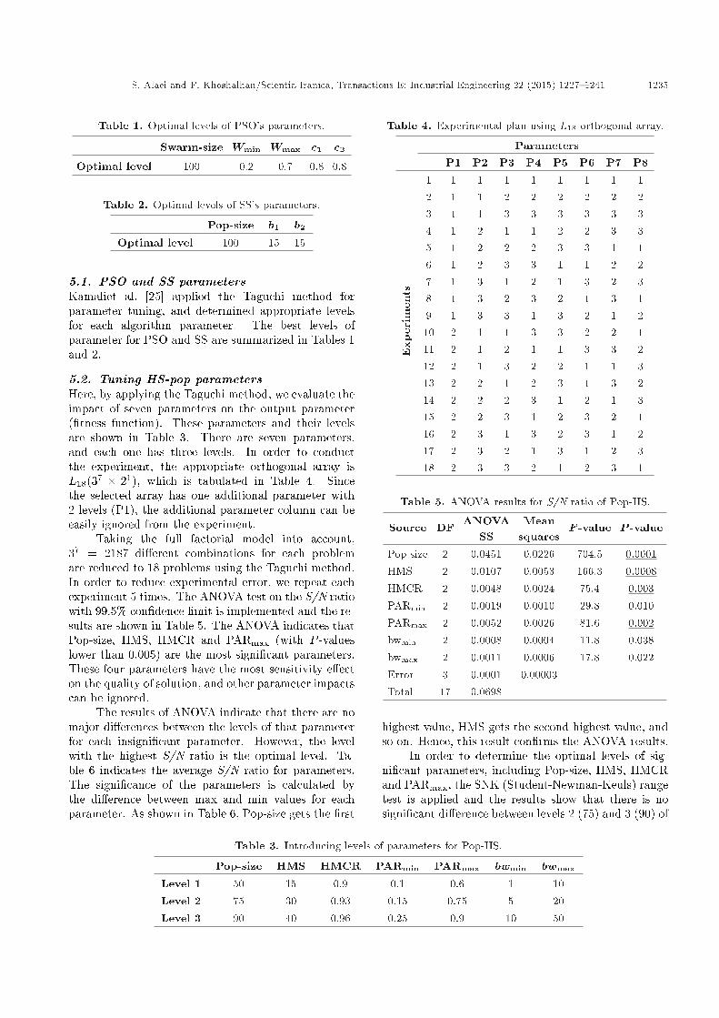
5.1. PSO and SS parametersKamaliet al. [25] applied the Taguchi method forparameter tuning, and determined appropriate levelsfor each algorithm parameter. The best levels ofparameter for PSO and SS are summarized in Tables 1and 2.

5.2. Tuning HS-pop parametersHere, by applying the Taguchi method, we evaluate theimpact of seven parameters on the output parameter(�tness function). These parameters and their levelsare shown in Table 3. There are seven parameters,and each one has three levels. In order to conductthe experiment, the appropriate orthogonal array isL18(37 � 21), which is tabulated in Table 4. Sincethe selected array has one additional parameter with2 levels (P1), the additional parameter column can beeasily ignored from the experiment.

Taking the full factorial model into account,37 = 2187 di�erent combinations for each problemare reduced to 18 problems using the Taguchi method.In order to reduce experimental error, we repeat eachexperiment 5 times. The ANOVA test on the S/N ratiowith 99.5% con�dence limit is implemented and the re-sults are shown in Table 5. The ANOVA indicates thatPop-size, HMS, HMCR and PARmax (with P -valueslower than 0.005) are the most signi�cant parameters.These four parameters have the most sensitivity e�ecton the quality of solution, and other parameter impactscan be ignored.

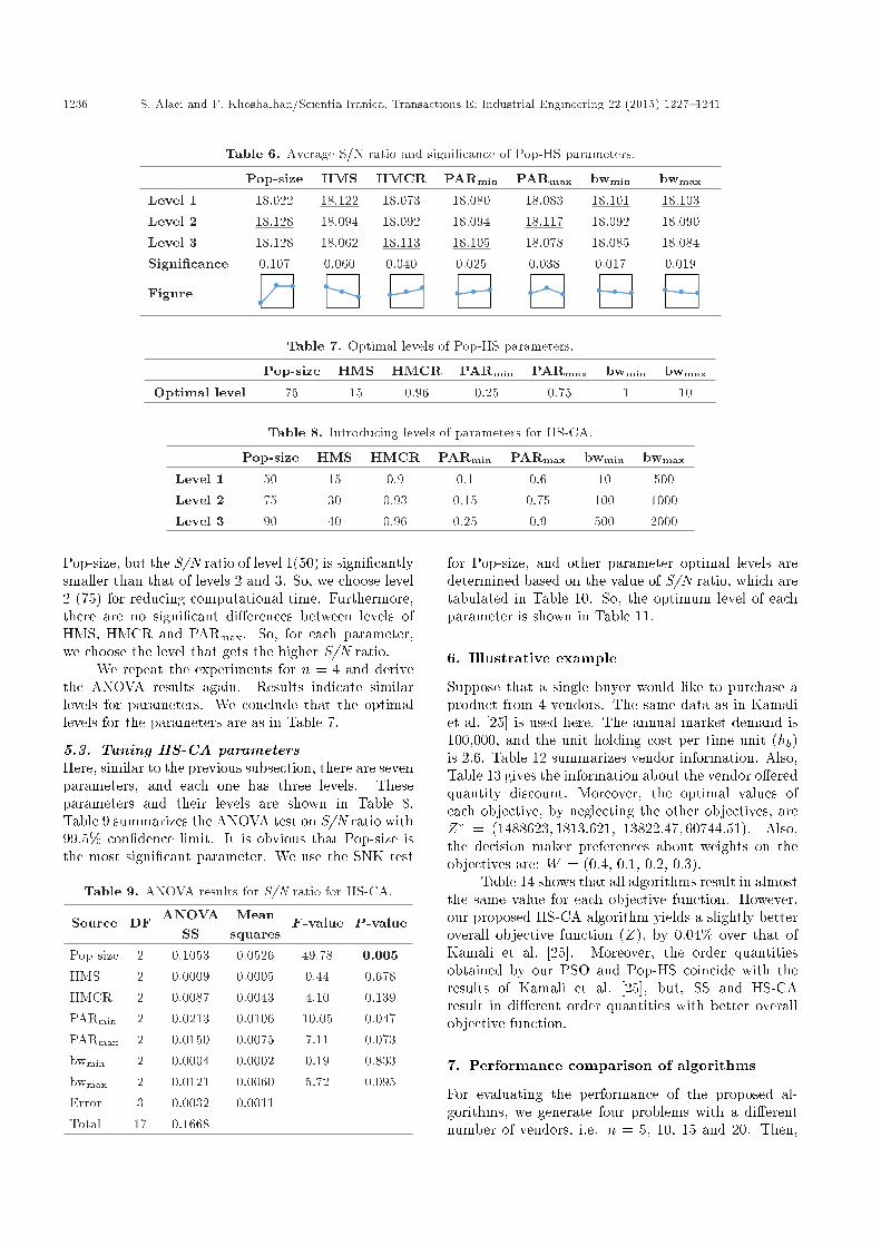
The results of ANOVA indicate that there are nomajor di�erences between the levels of that parameterfor each insigni�cant parameter. However, the levelwith the highest S/N ratio is the optimal level. Ta-ble 6 indicates the average S/N ratio for parameters.The signi�cance of the parameters is calculated bythe di�erence between max and min values for eachparameter. As shown in Table 6, Pop-size gets the �rst

Table 4. Experimental plan using L18 orthogonal array.

ParametersP1 P2 P3 P4 P5 P6 P7 P8

Exp

erim

ents

1 1 1 1 1 1 1 1 12 1 1 2 2 2 2 2 23 1 1 3 3 3 3 3 34 1 2 1 1 2 2 3 35 1 2 2 2 3 3 1 16 1 2 3 3 1 1 2 27 1 3 1 2 1 3 2 38 1 3 2 3 2 1 3 19 1 3 3 1 3 2 1 210 2 1 1 3 3 2 2 111 2 1 2 1 1 3 3 212 2 1 3 2 2 1 1 313 2 2 1 2 3 1 3 214 2 2 2 3 1 2 1 315 2 2 3 1 2 3 2 116 2 3 1 3 2 3 1 217 2 3 2 1 3 1 2 318 2 3 3 2 1 2 3 1

Table 5. ANOVA results for S/N ratio of Pop-HS.

Source DF ANOVASS

Meansquares

F -value P -value

Pop-size 2 0.0451 0.0226 704.5 0:0001HMS 2 0.0107 0.0053 166.3 0:0008HMCR 2 0.0048 0.0024 75.4 0:003PARmin 2 0.0019 0.0010 29.8 0.010PARmax 2 0.0052 0.0026 81.6 0:002bwmin 2 0.0008 0.0004 11.8 0.038bwmax 2 0.0011 0.0006 17.8 0.022Error 3 0.0001 0.00003Total 17 0.0698

highest value, HMS gets the second highest value, andso on. Hence, this result con�rms the ANOVA results.

In order to determine the optimal levels of sig-ni�cant parameters, including Pop-size, HMS, HMCRand PARmax, the SNK (Student-Newman-Keuls) rangetest is applied and the results show that there is nosigni�cant di�erence between levels 2 (75) and 3 (90) of

Table 3. Introducing levels of parameters for Pop-HS.

Pop-size HMS HMCR PARmin PARmax bwmin bwmax

Level 1 50 15 0.9 0.1 0.6 1 10Level 2 75 30 0.93 0.15 0.75 5 20Level 3 90 40 0.96 0.25 0.9 10 50


Table 6. Average S/N ratio and signi�cance of Pop-HS parameters.


Level 1 18.022 18:122 18.073 18.080 18.083 18:101 18:103Level 2 18:128 18.094 18.092 18.094 18:117 18.092 18.090Level 3 18.128 18.062 18:113 18:105 18.078 18.085 18.084Signi�cance 0.107 0.060 0.040 0.025 0.038 0.017 0.019

Figure

Table 7. Optimal levels of Pop-HS parameters.


Optimal level 75 15 0.96 0.25 0.75 1 10

Table 8. Introducing levels of parameters for HS-CA.


Level 1 50 15 0.9 0.1 0.6 10 500Level 2 75 30 0.93 0.15 0.75 100 1000Level 3 90 40 0.96 0.25 0.9 500 2000

Pop-size, but the S/N ratio of level 1(50) is signi�cantlysmaller than that of levels 2 and 3. So, we choose level2 (75) for reducing computational time. Furthermore,there are no signi�cant di�erences between levels ofHMS, HMCR and PARmax. So, for each parameter,we choose the level that gets the higher S/N ratio.

We repeat the experiments for n = 4 and derivethe ANOVA results again. Results indicate similarlevels for parameters. We conclude that the optimallevels for the parameters are as in Table 7.

5.3. Tuning HS-CA parametersHere, similar to the previous subsection, there are sevenparameters, and each one has three levels. Theseparameters and their levels are shown in Table 8.Table 9 summarizes the ANOVA test on S/N ratio with99.5% con�dence limit. It is obvious that Pop-size isthe most signi�cant parameter. We use the SNK test

Table 9. ANOVA results for S/N ratio for HS-CA.

Source DF ANOVASS

Meansquares

F -value P -value

Pop-size 2 0.1053 0.0526 49.78 0.005HMS 2 0.0009 0.0005 0.44 0.678HMCR 2 0.0087 0.0043 4.10 0.139PARmin 2 0.0213 0.0106 10.05 0.047PARmax 2 0.0150 0.0075 7.11 0.073bwmin 2 0.0004 0.0002 0.19 0.833bwmax 2 0.0121 0.0060 5.72 0.095Error 3 0.0032 0.0011Total 17 0.1668

for Pop-size, and other parameter optimal levels aredetermined based on the value of S/N ratio, which aretabulated in Table 10. So, the optimum level of eachparameter is shown in Table 11.

6. Illustrative example

Suppose that a single buyer would like to purchase aproduct from 4 vendors. The same data as in Kamaliet al. [25] is used here. The annual market demand is100,000, and the unit holding cost per time unit (hb)is 2.6. Table 12 summarizes vendor information. Also,Table 13 gives the information about the vendor o�eredquantity discount. Moreover, the optimal values ofeach objective, by neglecting the other objectives, areZ� = (1488623; 1813:621; 13822:47; 60744:51). Also,the decision maker preferences about weights on theobjectives are: W = (0.4, 0.1, 0.2, 0.3).

Table 14 shows that all algorithms result in almostthe same value for each objective function. However,our proposed HS-CA algorithm yields a slightly betteroverall objective function (Z), by 0.04% over that ofKamali et al. [25]. Moreover, the order quantitiesobtained by our PSO and Pop-HS coincide with theresults of Kamali et al. [25], but, SS and HS-CAresult in di�erent order quantities with better overallobjective function.

7. Performance comparison of algorithms

For evaluating the performance of the proposed al-gorithms, we generate four problems with a di�erentnumber of vendors, i.e. n = 5, 10, 15 and 20. Then,


Table 10. Average S/N ratio and signi�cance of HS-CA parameters.


Level 1 17.901 18:016 18:035 18:055 18:043 18:015 18.026Level 2 18.049 18.01 18.008 17.996 17.972 18.006 18:027Level 3 18:075 17.998 17.981 17.973 18.009 18.004 17.972Signi�cance 0.174 0.018 0.054 0.082 0.071 0.011 0.055

Figure

Table 11. Optimal levels of HS-CA parameters.


Optimal level 75 15 0.9 0.1 0.6 10 1000

Table 12. Vendors' information.

Vendor1 2 3 4

z 4.04 6.48 7.17 5.87S 43 39 42 30P 35108 29898 35785 68777A 40 19 25 39h 2.29 1.96 2.74 0.54d 0.0344 0.0551 0.0121 0.0215H 0.1444 0.1806 0.116 0.1581w 0.7968 0.3629 0.326 0.505

we run each algorithm ten times for each problem. Inorder to assess the quality of solutions, we use theRelative Percentage Deviation (RPD) as a performancemeasure, that is:

RPD =f� � ff� � 100; (34)

where f� is the global optimum or best known solution,and f is an obtained solution for an instance. Table 15shows the objective function values. It can be inferredfrom Table 15 that the HS-pop and HS-CA performbetter than standard HS, and they all perform betterthan SS and PSO in �nding best solutions. In order tobetter compare each algorithm performance, the RPDof each algorithm for each problem size is computedand illustrated by a box plot, as in Figure 4.

It can be implied from Figure 4 that HS-pop andHS-CA perform better than Scatter Search and ParticleSwarm optimization algorithms; both in best knownsolutions and solution variability.

In order to evaluate the computational time of theproposed algorithms, the time to reach a solution withr% error is computed, where r is the maximum value ofaverage RPD of di�erent algorithms for given n. Thevalue of r for n = 5, 10, 15 and 20 is equal to 7.8, 7.7,9.2 and 9.4, respectively. We de�ne the Convergence

Table 13. Discount intervals o�ered by vendors.

Vendor Intervals Unit prices

1

(0, 5000) 9[5000, 10000) 8.9[10000, 15000) 8.8[15000, 20000) 8.7[20000, 25000) 8.6[25000, 30000) 8.5[30000, 35108) 8.4

2

[0, 2000) 9.1[2000, 4000) 9[4000, 6000) 8.9[6000, 8000) 8.8[8000, 10000) 8.7[10000, 20000) 8.6

3

[0, 3000) 8.7[3000, 6000) 8.6[6000, 9000) 8.5[9000, 12000) 8.4[12000, 15000) 8.3[15000, 18000) 8.2[18000, 21000) 8.1[21000, 30000) 8

4

[0, 4000) 10.5[4000, 8000) 10.4[8000, 12000) 10.3[12000, 16000) 10.2[16000, 68777) 10.1

Index (CI) as the number of successful runs in whichthe algorithm reaches a solution with r% error in a timeless than 300 seconds, over the total number of runs.

CI =number of successful runs

total number of runs: (35)

All the algorithms are coded in MATLAB 2012 and run


Table 14. Optimal solution for base data.

HS Pop-HS HS-CA SS PSO Kamali et al. [25]

Z 0.063098 0.063098 0.063064 0.063087 0.063095 0.063095

Z1(�106) 1.5128 1.5128 1.5127 1.5127 1.5128 1.5128

Z2(�106) 0.0023 0.0023 0.0023 0.0023 0.0023 0.0023

Z3(�106) 0.0138 0.0138 0.0138 0.0138 0.0138 0.0138

Z4(�106) 0.0543 0.0543 0.0543 0.0543 0.0543 0.0543

Q1 5890 5890 2943 2972 5887 5887

Q2 0 0 0 0 0 0

Q3 6004 6004 3000 3030 6000 6000

Q4 4884 4884 2440 2465 4881 4880

Table 15. Computational results of the proposed algorithms.

nPSO SS HS-pop HS-CA HS

fmin �f fmin �f fmin �f fmin �f fmin �f

5 0.04861 0.0524 0.04868 0.04925 0.04861 0.04862 0.04861 0.04861 0.04861 0.04864

10 0.10519 0.10814 0.1028 0.10499 0.10045 0.10056 0.10044 0.10045 0.10053 0.10080

15 0.12271 0.12396 0.1198 0.12263 0.11367 0.11479 0.11357 0.11521 0.11402 0.11569

20 0.12613 0.13425 0.13139 0.13468 0.12331 0.12398 0.12309 0.12427 0.12409 0.12551

Figure 4. RPD of the proposed algorithms for a) n = 5, b) n = 10, c) n = 15, and d) n = 20.

on an Intel Core i3 2.10 GHz, HP Pavilion g6 at 4 GBRAM under a Microsoft Windows 7 environment. Werun each algorithm 20 times and results are tabulatedin Table 16. Note that the CPU time represents theaverage elapsing time of the algorithm in successfulruns.

It is obvious from Table 16 that HS-pop and HS-CA signi�cantly perform better than PSO and SS inboth convergence index and CPU time. Moreover,there is no distinguishable di�erence between HS-pop and HS-CA. In order to make a comprehensivecomparison between standard HS, HS-pop and HS-


Table 16. CPU time and convergence index of the proposed algorithms.

nPSO SS HS-pop HS-CA HS

CI CPU CI CPU CI CPU CI CPU CI CPU

5 70% 0.75 100% 0.41 100% 0.015 100% 0.015 100% 0.034

10 60% 1.3 90% 3.2 100% 0.020 100% 0.022 100% 0.053

15 55% 3.5 70% 4.9 100% 0.032 100% 0.031 100% 0.095

20 65% 5.6 40% 13.3 100% 0.038 100% 0.041 100% 0.255

Table 17. CPU time and convergence index of HS-pop and HS-CA.

nr = 3% r = 1%

HS-pop HS-CA HS HS-pop HS-CA HS

CI CPU CI CPU CI CPU CI CPU CI CPU CI CPU

5 100% 0.025 100% 0.027 100% 0.102 100% 0.076 100% 0.044 100% 0.619

10 100% 0.026 100% 0.043 100% 0.138 100% 0.070 100% 0.073 100% 2.890

15 90% 0.046 80% 0.061 80% 3.693 90% 1.323 35% 0.178 55% 4.922

20 100% 0.303 80% 0.095 90% 5.735 80% 1.180 25% 0.228 50% 7.923

Figure 5. \CPU time-problem size" curve foroptimization techniques.

CA, we run these algorithms again for r = 1% andr = 3%. Table 17 shows the results. It can be inferredfrom Table 17 that although there is no considerabledi�erence between the CPU times of the two algo-rithms, obviously, HS-pop performs better than HS-CAin convergence. Moreover, the standard HS takes muchmore CPU time to converge the solution.

We provide the \CPU time-problem size" curvefor all optimization techniques. As shown in Figure 5,HS-CA and HS-pop have a better performance thanstandard HS, and they all perform better than SS andPSO.

8. Conclusion

Due to the existence of competition and market pres-sure, coordinating all entities within a supply chain is

becoming increasingly critical. Some models have beendeveloped to investigate the coordination problem,together with the vendor selection problem. However,little attention has been paid to developing e�cientalgorithms in this area. By applying the GlobalCriterion method, the multi-objective mixed integernonlinear mathematical model is transformed into asingle objective optimization problem. Due to the com-plexity of the problem, we propose four metaheuristics:PSO, SS, and two hybrid algorithms, i.e., HS-pop andHS-CA. Then, the comparison is performed amongthe parameter-tuned algorithms. Solving the sampleproblems, it is shown that the modi�ed harmony searchalgorithms (HS-pop and HS-CA) have better perfor-mance than standard HS and they all perform betterthan SS and PSO in �nding high quality solutions inless computational time.

References

1. Thomas, D.J. and Gri�n, P.M. \Coordinated supplychain management", Eur. J. Oper. Res., 94(1), pp. 1-15 (1996).

2. Shin, H. and Tunca, T.I. \Do �rms invest in forecastinge�ciently? The e�ect of competition on demandforecast investment and supply chain coordination",Oper. Res., 58, pp. 1592-1610 (2010).

3. Fauli-Oller, R. and Sandonis, J. \Optimal two parttari� licensing contracts with di�erentiated goods andendogenous R&D", University of Allicante (2007).

4. Donohue, K.L. \E�cient supply contracts for fashiongoods with forecast updating and two productionmodels", Manag. Sci., 46, pp. 1397-1411 (2000).

5. Cachon, G.P. and Lariviere, M. \Supply chain coordi-


nation with revenue sharing contracts: Strengths andlimitations", Manag. Sci., 51, pp. 30-44 (2005).

6. Tsay, A.A. \The quantity exibility contract andsupplier-customer incentives", Manag. Sci., 45, pp.1339-1358 (1999).

7. Eppen, G.D. and Iyer, A.V. \Backup agreements infashion buying - the value of upstream exibility",Manag. Sci., 43, pp. 1469-1484 (1997).

8. Taylor, T.A. \Supply chain coordination under channelrebates with sales e�ort e�ects", Manag. Sci., 48, pp.992-1007 (2002).

9. Li, X. and Wang, Q. \Coordination mechanisms ofsupply chain systems", Eur. J. Oper. Res., 179, pp.1-16 (2007).

10. Sarlak, R. and Nookabadi, A. \Synchronization inmulti-echelon supply chain applying timing discount",Int. J. Adv. Manuf. Technol., 59, pp. 289-297 (2012).

11. Pezeshki, Y., Baboli, A. and Akbari-Jokar, M.R.\Simultaneous coordination of capacity building andprice decisions in a decentralized supply chain", Int.J. Adv. Manuf. Technol., 64, pp. 961-976 (2013).

12. Florez-Lopez, R. \Strategic supplier selection in theadded-value perspective: A CI approach", Inf. Sci.,177(5), pp. 1169-1179 (2007).

13. Rosenthal, E.C., Zydiak, J.L. and Chaudhry, S.S.\Vendor selection with bundling", Dec. Sci., 26, pp.35-48 (1995).

14. Sarkis, J. and Semple, J.H. \Vendor selection withbundling: A comment", Dec. Sci., 30(1), pp. 265-271(1999).

15. Goossens, D.R., Maas, A.J.T., Spieksma, F.C.R. andKlundert, J.J. \Exact algorithms for procurementproblems under a total quantity discount structure",Eur. J. Oper. Res., 178, pp. 603-626 (2007).

16. Ghodsypour, S.H. and O'Brien, C. \A decision sup-port system for supplier selection using an integratedanalytic hierarchy process and linear programming",Int. J. Prod. Econ., 56, pp. 199-212 (1998).

17. Amid, A., Ghodsypour, S.H. and O'Brien, C. \Aweighted additive fuzzy multi-objective model for thesupplier selection problem under price breaks in asupply chain", Int. J. Prod. Econ., 121, pp. 323-332(2009).

18. Jayaraman, V., Srivastava, R. and Benton, W.C.\Supplier selection and order quantity allocation: Acomprehensive model", J. Suppl. Chain Manag., 35,pp. 50-58 (1999).

19. Cakravastia, A., Toha, I.S. and Nakamura, N. \A two-stage model for the design of supply chain network",Int. J. Prod. Econ., 80, pp. 231-248 (2002).

20. Dahel, N.E. \Vendor selection and order quantityallocation in volume discount environments", Suppl.Chain Manag.: Int. J., 8(4), pp. 335-342 (2003).

21. Xia, W. and Wu, Z.H. \Supplier selection with multi-

ple criteria in volume discount environments", Omega,35, pp. 494-504 (2007).

22. Ebrahim, R.M., Razmi, J. and Haleh, H. \Scattersearch algorithm for supplier selection and order lotsizing under multiple price discount environment",Adv. Eng. Soft., 40, pp. 766-776 (2009).

23. Herer, Y.T., Rosenblatt, M.J. and Hefter, I. \Fastalgorithms for single-sink �xed charge transportationproblems with applications to manufacturing andtransportation", Transport. Sci., 30(4), pp. 276-290(1996).

24. Kim, T. and Goyal, S.K. \A consolidated deliverypolicy of multiple suppliers for a single buyer", Int.J. Proc. Manag., 2, pp. 267-287 (2009).

25. Kamali, A., Fatemi-Ghomi, S.M.T. and Jolai, F. \Amulti-objective quantity discount and joint optimiza-tion model for coordination of a single-buyer multi-vendor supply chain", Comput. Math. Appl., 62, pp.3251-3269 (2011).

26. Gheidar-Kjeljani, J., Ghodsypour, S.H. and Fatemi-Ghomi, S.M.T. \Supply chain optimization policy fora supplier selection problem: a mathematical program-ming approach", Iran. J. Oper. Res., 2(1), pp. 17-31(2010).

27. Eberhart, R.C. and Kennedy, J. \A new optimizerusing particle swarm theory", In Proceedings of theSixth International Symposium on Micro Machine andHuman Science, Nagoya, Japan, pp. 39-43 (1995).

28. Kennedy, J. and Eberhart, R.C. \Particle swarmoptimization", In IEEE International Conference onNeural Networks, Perth, Australia, pp. 1942-1948(1995).

29. Glover, F. \Heuristics for integer programming us-ing surrogate constraints", Dec. Sci., 8, pp. 156-166(1977).

30. Laguna, M. and Marti, R., Scatter Search: Method-ology and Implementations, in C. Kluwer AcademicPublishers, Boston, MA (2003).

31. Marti, R., Laguna, M. and Glover, F. \Principles ofscatter search", Eur. J. Oper. Res., 169(2), pp. 359-372 (2006).

32. Geem, Z.W., Kim, J.H. and Loganathan, G. \A newheuristic optimization algorithm: Harmony search",Simulation, 76(2), pp. 60-68 (2001).

33. Mahdavi, M., Fesanghary, M. and Damangir, E. \Animproved harmony search algorithm for solving opti-mization problems", Appl. Math. Comput., 188(2), pp.1567-1579 (2007).

34. Reynolds, R.G. \An introduction to cultural algo-rithms", In Proceedings of the 3rd Annual Conferenceon Evolutionary Programming, World Scienti�c Pub-lishing, San Diego, Calif, USA, pp. 131-139 (1994).

35. Srinivasan, S. and Ramakrishnan, S. \Cultural algo-rithm toolkit for interactive knowledge discovery", Int.


J. Data Mining & Knowledge Manage. Process, 2(5),pp. 53-70 (2012).

36. Sternberg, M. and Reynolds, R.G. \Using culturalalgorithms to support re-engineering of rule basedexpert systems in dynamic environments: A case studyin fraud detection", IEEE Trans. Evol. Comput., 1(4),pp. 225-243 (1997).

37. Gao, X.Z., Wang, X., Jokinen, T., Ovaska, S.J.,Arkkio, A. and Zenger, K. \A hybrid optimizationmethod for wind generator design", Int. J. Innov.Comput. Inf. Control, 8(6), pp. 4347-4373 (2012).

Biographies

Saeed Alaei obtained BS and MS degrees in IndustrialEngineering from Amirkabir University of Technology,

Tehran, Iran, in 2009, and Sharif University of Technol-ogy, Tehran, Iran, in 2011, respectively. He is currentlya PhD degree candidate in Industrial Engineering atK.N. Toosi University of Technology, Tehran, Iran. Hisresearch interests are mainly focused on supply chaincoordination, multi-echelon inventory management andgame theory.

Farid Khoshalhan received MS and PhD degrees inIndustrial Engineering, in 1997 and 2001, respectively,from Tarbiat Modares University, Tehran, Iran. Heis currently Assistant Professor in the Faculty of In-dustrial Engineering at K.N. Toosi University of Tech-nology, Tehran, Iran. His research interests include e-commerce and e-business, evolutionary algorithms andmetaheuristics, multiple criteria decision making andgame theory.

a hybrid cultural-harmony algorithm for multi-objective...

Documents