on the gravity recommendation system
TRANSCRIPT

On the Gravity Recommendation System
Gabor TakacsDept. of Measurement and
Information SystemsBudapest University of
Technology and EconomicsMagyar Tudosok krt. 2.
Budapest, [email protected]
Istvan PilaszyDept. of Measurement and
Information SystemsBudapest University of
Technology and EconomicsMagyar Tudosok krt. 2.
Budapest, [email protected]
Bottyan NemethDept. of Telecom. and Media
InformaticsBudapest University of
Technology and EconomicsMagyar Tudosok krt. 2.
Budapest, [email protected]
Domonkos TikkDept. of Telecom. and Media
InformaticsBudapest University of
Technology and EconomicsMagyar Tudosok krt. 2.
Budapest, [email protected]
ABSTRACTThe Netflix Prize is a collaborative filtering problem. Thissubfield of machine learning has become popular from thelate 1990s with the spread of online services that use rec-ommendation systems, such as e.g. Amazon, Yahoo! Mu-sic, and of course Netflix. The aim of such a system is topredict what items a user might like based on his/her andother users previous ratings. The dataset of Netflix Prizeis much larger than the previously known benchmark sets,therefore we first show in the paper how to store it efficientlyand adaptively to various algorithms. Then we describe theoutline of our solution, called the Gravity RecommendationSystem (GRS), to the Netflix Prize contest, which is in theleader position with RMSE 0.8808 at the time of the submis-sion of the paper. GRS comprises of the combination of dif-ferent approaches that are presented in the main part of thepaper. We then compare the effectiveness of some selectedindividual and combined approaches against a designatedsubset of the dataset, and discuss their important featuresand drawbacks. Beside the description of successful experi-ments we also report on the useful lessons of (temporarily)failed ideas and algorithms.
Categories and Subject DescriptorsH.5.3 [Information Storage and Retrieval]: InformationSearch and Retrieval—Information Filtering ; G.3 [Probabilityand Statistics]: Correlation and regression analysis
Permission to make digital or hard copies of all or part of this work forpersonal or classroom use is granted without fee provided that copies arenot made or distributed for profit or commercial advantage and that copiesbear this notice and the full citation on the first page. To copy otherwise, torepublish, to post on servers or to redistribute to lists, requires prior specificpermission and/or a fee.KDD Cup Workshop at SIGKDD ’07 San Jose, California USACopyright 200X ACM X-XXXXX-XX-X/XX/XX ... $5.00.
General TermsExperimentation, Algorithms
KeywordsNetflix Prize, Machine learning, Collaborative filtering, Ma-trix factorization
1. INTRODUCTIONCollaborative filtering (CF) is a subfield of machine learn-
ing that aims at creating algorithms to predict user prefer-ences based on known user ratings or user behavior in selec-tion/purchasing items. Such a system has great importancein applications in e-commerce, subscription based services,information filtering and so on. Recommendation systemsproviding personalized suggestions greatly increase the like-lihood over a customer making a purchase than unperson-alized ones. This is especially important on such a marketwhere the variety of choices is large, the taste of the cus-tomer is important, and last but not least the price of theitems is modest. Typical areas of such services are mostlyrelated to art (esp. books, movies, music), fashion, food &restaurants, gaming & humor, etc. Clearly, the online DVDrental service operated by Netflix fits into this list.
The Netflix Prize problem (see the details in the generaldescription, [2]) belongs to one of the typical framework ofCF called the social-filtering method. In this case the userfirst provides ratings of some items, titles or artifacts usuallyon a discrete numerical scale, and then the system recom-mends other items based on ratings the virtual communityusing the system has already provided. The virtual com-munity was defined in [6] as “a group of people who sharecharacteristics and interact in essence or effect only” that isin reality they do not interact. The underlying assumptionof such a system that people who had similar taste in thepast may also agree in the future.
1.1 Related works
22

The first works on the field of CF has been publishedfrom early 1990s. The GroupLens systems of [10] was one ofthe pioneer applications of the field where users could ratearticles after reading on a 1–5 scale, and then were offeredsuggestion. The underlying techniques of predicting userpreferences can be divided into two main groups [3]. Thememory based approaches operate on the entire databaseof ratings collected by the vendor or service supplier. Onthe other hand, model based approaches use the database toestimate or learn a model, and then apply it for prediction.
Over the last broad decade many CF algorithms havebeen proposed that approach the problem from differentpoint of view, including similarity based approaches [10, 13],Bayesian networks [3], personality diagnosis [8], various ma-trix factorization techniques [4, 7, 12, 16], and very recentlyrestricted Boltzman machines [11]. Short descriptions of themost important CF algorithm can be found in [1], while in[3] a more detailed survey is given on major CF approaches.The GRS described in this paper apply the combinationof several different approaches to maximize its performance(see details in Section 3).
1.2 The aim of this paperAs we have experienced in the last few months, the de-
velopment of a high-quality movie recommender system isnot only about innovative approaches and tricky ideas butit also requires a lot of efficient coding and experimentationin order to try different variants of approaches and para-meter settings, resp. Even after a superficial scanning ofthe related literature, one can easily find that the matrixfactorization and the K-nearest neighbors approaches suitswell to the Netflix Prize problem. We also believe that manyother teams use these methods in their prediction algorithm.However, a good approach does not necessarily guarantee agood implementation. This latter additionally requires towork out every minor detail of the algorithm appropriately,which is laborious and cumbersome.
In this paper, we present the main components of oursolution termed Gravity Recommendation Systems to theNetflix Prize and show how the individual methods are com-bined to obtain more efficient results. However, due to thelimits of the paper and our obvious interests, we intention-ally do not publish all parts of the puzzle: some small butimportant details remain hidden.
1.3 OrganizationThis paper is organized as follows. Section 2 deals with
the data storage issue after having introduced the notationsand some formulae used throughout the paper. Section 3describes the algorithms we have experimented with andapplied in GRS. Section 4 presents the result achieved bymeans of the presented approaches, which is followed by aconcise discussion.
2. PRELIMINARIES
2.1 NotationWe use the following notation in this paper. The rating
matrix is denoted by X ∈ {1, . . . , 5}I×J , where an elementxij stores the rating of the jth movie provided by ith cus-tomer. I and J denote the total number of users and movies,resp. We refer to the set of all known (i, j) pairs in X as R.At the prediction of a given rating we refer to the user as
active user, and to the movie as active movie. Superscript,,hat” denotes the prediction of the given quantity, that is xis the prediction of x.
Concerning the details of the Netflix Prize problem (e.g.the terminology of various datasets), we refer the Reader tothe general description given in [2].
2.2 Data storageNetflix has generously provided a 100 million ratings data-
set for the contestants. Because the size of the training setis huge compared to other benchmark problems of collabo-rative filtering and in the usual machine learning tasks, thestorage of training data is an important issue. For compari-son the widespreadly used EachMovie dataset1 only consistsof about 2.8 million ratings of 73k users and 1628 movies.Another dataset of the GroupLens project (see e.g. [1]) hasabout 13 million ratings from 105k users on 9k movies.
Efficient data storage is particularly important since theoriginal format of the database is impractical: reading andparsing the text files takes about 30 minutes with by meansa naive implementation. It is crucial to reduce the ex-perimenting time in order to speed up the development.The weakness of model-based approaches, namely that themodel-building process is time-consuming [1], can also beeliminated or degraded with proper implementation. Thetime requirement of both the input processing and the learn-ing/predicting phases can be reduced with several ordersof magnitude by means of an appropriate representation ofdata described next.
Clearly, it is worth storing the entire training set in thememory, if it is possible. Consequently, we decided to trans-form the original input data into a concise binary format.Based on some experiments, we found that the date of theratings can be thrown away. Because the 99 percent of rat-ings in the movie-user matrix is unknown, it is practical touse sparse representation. There are two reasonable choices:
• The per-user storage represents each row as a list of(column index, value) pairs.
• The per-movie storage represents each column as a listof (row index, value) pairs.
In the first case it is easy to go through the ratings of agiven customer. In the second case the ratings of a moviecan be queried efficiently. Most algorithms prefer the firstrepresentation, some prefer the second one, and some meth-ods need both. It is also possible to store the matrix as (rowindex, column index, value) triplets, but this is impracticalbecause it provides none of the above advantages.
In the training database there are 480189 customers and17770 movies, so the space requirement of the row index andthe column index is 19 bits and 15 bits, resp. The 5 differentvalues of the ratings can be stored in 3 bits. Therefore thespace requirement of one matrix element is 18 bits in the per-user and 22 bits in the per-movie representation. In practicethis means that with appropriate C structs (see Table 1) arating can be stored in 24 bits and the storage of the wholematrix requires ∼300 MB in each case.
This database representation made us possible to developefficient algorithms on an average PC. We achieved our first
1It used to be available upon request from Compaq, but in2004 the proprietary retired the dataset, and since then itis no longer available for download.
23

Table 1: C structures for storing one ratingstruct PerUserRating { struct PerMovieRating {ushort movieId; uchar userIdxHi;
uchar value; uchar userIdxLo:4;
}; uchar value:4;
};
leading position using only a 2 GHz notebook with 1 GBRAM.
For a weaker hardware (512 MB RAM), the 300 MB rep-resentation can be still too large to work with. Therefore,we have developed an even more compact per-user represen-tation, which requires only 200 MB at the expense of a bitslower access to the data.
To achieve this, first we split the matrix into two halves.The first one contains ratings for movies with ID≤ 17770/2 =8885, the second contains the rest. We utilize the fact that8885 · 5 = 44425 ≤ 216 = 65536. This means, that a moviewith ID between 1 and 8885 and its rating between 1 and 5can be stored in 2 bytes:
(j, xij) → cij := 5 · j + xij − 1
cij → j = bcij/5c, xij = 1 + (cij mod5)
where j ∈ [1, J ] identifies the movie. Movies with ID > 8885can be treated similarly: first we subtract 8885 from the ID,then the rating and the new ID (≤ 8885) can be stored in 2bytes in the second matrix.
3. APPROACHES
3.1 Matrix factorizationThe idea behind matrix factorization (MF) techniques is
very simple. Suppose we want to approximate the matrixX as the product of two matrices:
X ≈ UM, (1)
where U is an I×K and M is a K×J matrix. The uik andmkj values can be considered, reps. the kth feature of the ithuser and the jth movie. If we consider the matrices as lineartransformations, the approximation can be interpreted asfollows: the M matrix transforms from V1 = RJ into V2 =RK , and U transforms from V2 into V3 = RI . Thus, the V2
vector space acts as a bottleneck when predicting v3 ∈ V3
from v1 ∈ V1. In other words, the number of parameters todescribe X is reduced from |R| to IK + KJ . However, Xcontains integers of range 1 to 5, while M and U containreal numbers.
Several matrix factorization techniques have been appliedsuccessfully to CF, including SVD (singular value decompo-sition, [12]), pLSA (probabilistic latent semantic analysis,[7]), and MMMF (maximum margin matrix factorization,[16]). Due to the speciality of the Netflix Prize problem, thesolution should be sought as a low-rank approximation withmissing data (see also e.g. [5, 9, 15]). Here we present thebasics of MF methods via SVD:
X = UΣM, (2)
where U ∈ RI×min(I,J) and M ∈ Rmin(I,J)×J are orthogo-nal matrices, and Σ ∈ Rmin(I,J)×min(I,J) contains non-zeroelements only along the diagonal. These elements are called
singular values, and are always non-negative. If we keeponly the K largest singular values and replace the othersby zero, we got X, a K-rank approximation of X with thefollowing property:
‖X−X‖ = min{‖X′ −X‖ : X′ ∈ RI×J , rank(X′) ≤ K}In other words: from the SVD the optimal K-rank approx-imation of X can easily be computed, which minimizes the
Frobenius norm, defined as ‖A‖ =qP
a∈A a2, of the dis-
tance of the matrices. We can eliminate Σ from the factor-ization given in eq. (2):
X = (UΣ)M = U(ΣM) = (U√
Σ)(√
ΣM),
thus the form reduces to eq. (1).In the case of the given problem, X has many unknown
elements which cannot be treated as zero. For this case,the approximation task can be defined as follows. Let nowU ∈ RI×K and M ∈ RK×J . Let uik denote the elements ofU, and mkj the elements of M. Then:
xij =
KXk=1
uikmkj (3)
eij = xij − xij for (i, j) ∈ R
SE =X
(i,j)∈Re2
ij =X
(i,j)∈R
xij −
KXk=1
uikmkj
!2
(U,M) = arg min(U,M)
SE (4)
Here xij denotes how the ith user would rate the jth movie,according to the model, eij denotes the training error on the(i, j)th example, and SE denotes the total squared trainingerror. Eq. (4) states that the optimal U and M minimizesthe sum of squared errors only on the known elements of X.
In order to minimize SE (which is equivalent to minimizeRMSE), we have applied a simple gradient descent methodto find a local minimum. Suppose that a training examplexij and its approximation xij are given. We compute thegradient of e2
ij :
∂
∂uike2
ij = −2eij ·mkj ,∂
∂mkje2
ij = −2eij · uik. (5)
We update the weights in the opposite direction of gradient:
u′ik = uik + η · 2eij ·mkj , m′kj = mkj + η · 2eij · uik,
that is, we change the weights in U and M to decrease theerror, thus better approximating xij . Here η is the learn-ing rate. To better generalize on unseen examples, we haveapplied regularization with factor λ to prevent large weights:
u′ik = uik + η · (2eij ·mkj − λ · uik) (6)
m′kj = mkj + η · (2eij · uik − λ ·mkj) (7)
Our algorithm can be summarized as follows:
1. Initialize the weights in U and M randomly.Set η and λ to some small positive value.
2. Loop until the terminal condition is met
(a) Iterate over each known element of X which isnot in the probe subset. For xij :
i. compute eij ;
24

ii. compute the gradient of e2ij ;
iii. update the ith row of U and the jth columnof M according to eqs. (6)–(7).
(b) Calculate the RMSE on the probe subset.
The loop is terminated when the RMSE does not decreaseduring two iterations.
Note that if the rows of U and the columns of M are con-stant vectors, each row of U and each column of M remainsa constant vector. That is, why we initialize randomly. Ourapproach is very similar to Simon Funk’s SVD,2 but we up-date each factor simultaneously, and initialize the matrixrandomly. Simon Funk’s approach learns the first factor fora certain number of iterations, then the second, and so on.His approach converges much slower than ours because ititerates more on X. Additionally, it is not specified in hisalgorithm when one has finish the learning of one factor andstart the next.
We remark that after the learning phase, each value of Xcan be computed easily by eq. (3), even the “unseen” values.In other words, the model (U and M) can say somethingabout how an arbitrary user would rate any movie.
GRS comprises of a combination of several methods. Amongthem there are some variants of the presented MF algorithm,which will be described next.
3.1.1 Using datesWe can easily incorporate the date of ratings into the MF
model. Let gij denote the date of the (i, j)th rating, repre-sented as an integer between 1 and L. We can then refor-mulate eq. (3) as
xij =
KXk=1
uikmkjdkl, where l = gij .
Here dkl are the elements of D ∈ RK×L. Its weights areinitialized randomly as well. We compute the gradient ofe2
ij = (xij − xij)2:
∂
∂uike2
ij = −2eij ·mkj · dkl,
∂
∂mkje2
ij = −2eij · uik · dkl,
∂
∂dkle2
ij = −2eij · uik ·mkj .
The weight updating scheme is similar to eqs. (6)–(7):
u′ik = uik + η · (− ∂
∂uik− λ · uik)
m′kj = mkj + η · (− ∂
∂mkj− λ ·mkj)
d′kl = dkl + η · (− ∂
∂dkl− λ · dkl)
This method can adapt to some changes in the users’ rat-ing conventions, which may be caused for example by pro-motions for users to rate more movies or by improvement inthe recommendation system. Although, these MF modelswith dates do not result a significant improvement of theprediction, they can be efficiently used in the combinationsince they differ sufficiently from regular MFs.
2http://sifter.org/~simon/journal/20061211.html
3.1.2 Constant values in matricesBeside the (user ID, movie ID, date, rating) quadruples,
Netflix has also provided the title and year of release ofeach movie. This information can be incorporated in theMF model as follows: we can extend M with rows thatindicate the occurrence of words in the movie title, or theyear of release. For example, the k1th row of M is 1 or0 depending on whether the term “Season” occurs in thetitle of the movies or not. This row of M is fixed to bea constant, thus we do not apply equ. (7) for k = k1. Ifthe occurrence of term “Season” in the title increases theith user’s rating (i.e. the user likes TV-series), the resultingmodel can have positive weight for uik1 . Other constantvalues can be inserted, for example, we can increase the sizeof matrices, K, with 2 by inserting the average rating of theuser and the movie, resp.
3.1.3 Rounding the valuesX contains only integers between 1 and 5, and this holds
also for the unknown ratings in the Quiz set. It is straight-forward that this information should also be exploited. Wehave tried several approaches to round the values in UM,but none of them helped. The error of approximation (ele-ments of X −UM) has Gaussian distribution, with µ = 0and σ between 0.7 and 1.0. Note that σ is the same as theRMSE in the Netflix contest, but on the training set. Be-cause a large portion of the errors are ≥ 0.5, rounding thevalues has no point. To see this, let us suppose that we wantto round the values with the following function:
x′ij = ρ · xij + (1− ρ) · round(xij) 0 ≤ ρ ≤ 1 (8)
If we set ρ to 1, there is no rounding, if we set to 0, we roundeach value to the closest integer. Errors between 0 and 0.5will decrease, errors between 0.5 and 1 will increase, between1 and 1.5 decrease, etc. For example, suppose that for somei, j, xij = 2, xij = 1.2, and ρ = 0.9. Hence, x′ij = 1.18and we increased the error by 0.02. Let ε = xij − xij andε′ = xij − x′ij denote the variate of training error before andafter rounding, resp. If −0.5 < ε < 0.5, then −0.5 · ρ < ε′ <0.5 ·ρ. If 0.5 < ε < 1.5, then 1−0.5 ·ρ < ε′ < 1+0.5 ·ρ, etc.
Let ϕ denote the probability density function of ε:
ϕ(x) =1√2πσ
exp
�− (x− µ)2
2σ2
�Formally, the training error after rounding will be:
RMSE =
vuutXn∈Z
Z n+0,5
n−0.5
ϕ(x) · (n + ρ(x− n))2 dx
When ρ = 0.9, this approach improves performance only ifσ is below ∼ 0.5, which seems unreachable (on the probesubset).
We have also tried another rounding approach, which de-fines a smooth rounding function as follows:
sr(x) = bxc+ tanh((x− bxc − 0.5) · 2 ·A)− tanh(−A)
tanh(A)− tanh(−A)(9)
Here A controls the “smoothness” of rounding.We can apply rounding functions (8) or (9) either on the
entire or on a part of the output, i.e.:
xij =
K1Xk=1
uikmkj + sr
0@ KXk=K1+1
uikmkj
1A ,
25

where 0 ≤ K1 < K denotes the part not altered by rounding.With this modification, the computation of the gradient, eq.(5), becomes more complicated.
We expected that this model will activate rounding onlyon such users for who this is worthwhile, and thus improvesthe performance. However, it yielded inferior results.
We tried to apply different non-linear functions on differ-ent parts of the output, but none of these experiments weresuccessful. The failure of these trials can be supported bythe following explanatory example. If xij is 4.1, then theuser would rate 4 with probability 0.9, and 5 with proba-bility 0.1, and the decision of the user is taken completelyarbitrarily.
3.1.4 Parameters of matrix factorizationThe more parameters a matrix factorization has, the harder
to set them well, but the more chance to get a better RMSE.We experimented with the following parameters:
• the number of features: K;
• different learning rate and regularization factor
– for users and movies;
– at different learning cycles;
– values of η and λ depends on k in eqs. (6)–(7);
– for users or movies with different number of rat-ings;
– for the corresponding variables of constant fea-tures;
• probability distribution function to initialize U andM;
• offset to subtract from X before learning (can be, e.g.,set to the global average of ratings);
• nonlinear functions on parts of the output as in eq. (9).
We subsampled the matrix for faster evaluation of a pa-rameter settings. We experienced that movie-subsamplingsubstantially increased the error, in contrast to user-subsampling.It is interesting, that the larger the subsample is, the feweriterations are required to achieve the optimal model. Wethink this is because of the redundancy in the data set.
3.1.5 Connections with neural networksThe MF model can be considered as the learning of a
multi-layer perceptron given on Figure 1. The network hasI inputs, J outputs and K hidden neurons, and identityactivation function in each neuron. We consider the weightbetween the ith input and the kth hidden neuron as uik,and the weight between the kth hidden neuron and the jthoutput neuron as mkj .
The network applies incremental learning method. For the(i, j)th rating, we set the input x as xi is 1 and xk 6=i = 0,thus zk = uik holds. Let xij = yj denote the jth outputof the network. We compute the error: eij = xij − xij .This error is back-propagated from the jth output neurontowards the input layer.
In the evaluation phase, we set the input as in the learningphase, and yj (j = 1, . . . , J) predicts the active user’s ratingon the jth movie. The network can be generalized in manyways, e.g.:
x2
x3
x1 y1
y2
y3
yJxI
z1
z2
zK
Figure 1: Multilayer perceptron for collaborative fil-tering
• reverse the direction of edges;
• replace some of the identity activation functions withnon-linear ones in the hidden layer or in the outputlayer;
• create more hidden layers;
• apply batch learning.
3.1.6 2D Modifications of the matrix factorizationalgorithm
The linear combination of different MF algorithms is bet-ter than the best single algorithm. The result is as goodas different the MFs are in the combination. Based on thisobservation, we made different modifications on simple MFmodels. In one experiment we arranged the movie and userfeatures (recall that these are provided by MF) to a 2Dlattice and defined a simple neighborhood relation betweenthe features. If the difference of the horizontal and verticalpositions of two features are small (they are neighbors) the“meaning” of those features should also be close. To achievethis, we proceed as follows. After each usual learning step,we modify the feature values towards the direction of theneighboring features by smoothing the calculated changesof feature values. In practice, in order to prevent slow train-ing, we take only those features into account which are nextto each other
∆u′i,k1,k2 = ∆ui,k1,k2 + ξ(∆ui,k1+1,k2 + ∆ui,k1−1,k2
+ ∆ui,k1,k2+1 + ∆ui,k1,k2−1) +ξ√2(∆ui,k1+1,k2+1
+ ∆ui,k1−1,k2−1 + ∆ui,k1−1,k2+1 + ∆ui,k1+1,k2−1).
Here ξ is the smoothing rate, ∆u′ the modified and ∆u the2D array of the original changes in user features. The indicesof ∆u denotes the user index, and the two coordinates of thefeature in the feature array, respectively. We applied analogformula also on the movies.
The 2D features of a movie (or user) can be nicely visu-alized. Meanings can be associated with the regions of theimage. The labels on Figure 2 are assigned to sets of fea-tures and not to single ones. The labels has been determinedbased on such movies that have extreme values at the givenfeature.
Such feature maps are useful for detecting main differencesbetween movies or episodes of the same movie. Figure 3
26
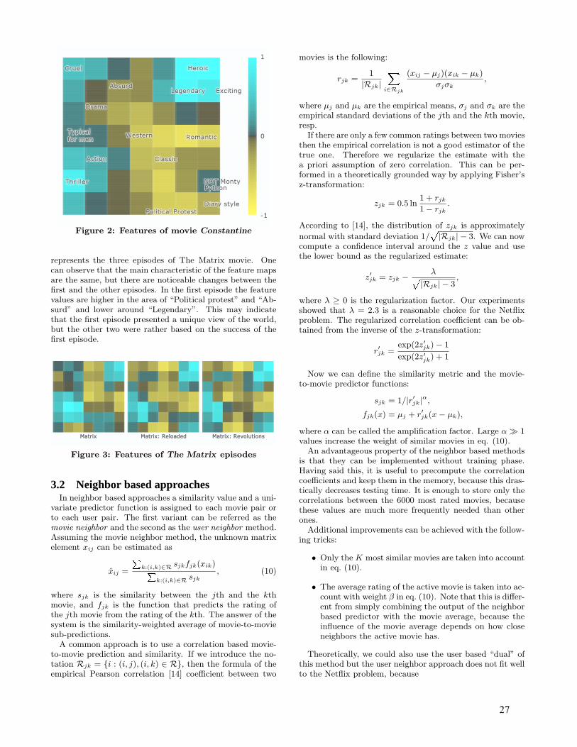
Figure 2: Features of movie Constantine
represents the three episodes of The Matrix movie. Onecan observe that the main characteristic of the feature mapsare the same, but there are noticeable changes between thefirst and the other episodes. In the first episode the featurevalues are higher in the area of “Political protest” and “Ab-surd” and lower around “Legendary”. This may indicatethat the first episode presented a unique view of the world,but the other two were rather based on the success of thefirst episode.
Figure 3: Features of The Matrix episodes
3.2 Neighbor based approachesIn neighbor based approaches a similarity value and a uni-
variate predictor function is assigned to each movie pair orto each user pair. The first variant can be referred as themovie neighbor and the second as the user neighbor method.Assuming the movie neighbor method, the unknown matrixelement xij can be estimated as
xij =
Pk:(i,k)∈R sjkfjk(xik)P
k:(i,k)∈R sjk, (10)
where sjk is the similarity between the jth and the kthmovie, and fjk is the function that predicts the rating ofthe jth movie from the rating of the kth. The answer of thesystem is the similarity-weighted average of movie-to-moviesub-predictions.
A common approach is to use a correlation based movie-to-movie prediction and similarity. If we introduce the no-tation Rjk = {i : (i, j), (i, k) ∈ R}, then the formula of theempirical Pearson correlation [14] coefficient between two
movies is the following:
rjk =1
|Rjk|X
i∈Rjk
(xij − µj)(xik − µk)
σjσk,
where µj and µk are the empirical means, σj and σk are theempirical standard deviations of the jth and the kth movie,resp.
If there are only a few common ratings between two moviesthen the empirical correlation is not a good estimator of thetrue one. Therefore we regularize the estimate with thea priori assumption of zero correlation. This can be per-formed in a theoretically grounded way by applying Fisher’sz-transformation:
zjk = 0.5 ln1 + rjk
1− rjk.
According to [14], the distribution of zjk is approximately
normal with standard deviation 1/p|Rjk| − 3. We can now
compute a confidence interval around the z value and usethe lower bound as the regularized estimate:
z′jk = zjk − λp|Rjk| − 3
,
where λ ≥ 0 is the regularization factor. Our experimentsshowed that λ = 2.3 is a reasonable choice for the Netflixproblem. The regularized correlation coefficient can be ob-tained from the inverse of the z-transformation:
r′jk =exp(2z′jk)− 1
exp(2z′jk) + 1
Now we can define the similarity metric and the movie-to-movie predictor functions:
sjk = 1/|r′jk|α,
fjk(x) = µj + r′jk(x− µk),
where α can be called the amplification factor. Large α À 1values increase the weight of similar movies in eq. (10).
An advantageous property of the neighbor based methodsis that they can be implemented without training phase.Having said this, it is useful to precompute the correlationcoefficients and keep them in the memory, because this dras-tically decreases testing time. It is enough to store only thecorrelations between the 6000 most rated movies, becausethese values are much more frequently needed than otherones.
Additional improvements can be achieved with the follow-ing tricks:
• Only the K most similar movies are taken into accountin eq. (10).
• The average rating of the active movie is taken into ac-count with weight β in eq. (10). Note that this is differ-ent from simply combining the output of the neighborbased predictor with the movie average, because theinfluence of the movie average depends on how closeneighbors the active movie has.
Theoretically, we could also use the user based “dual” ofthis method but the user neighbor approach does not fit wellto the Netflix problem, because
27

• user correlations are unreliable, since there are typi-cally very few common movies between two arbitraryusers;
• the distribution of the users is approximately uniformin the test set, therefore there is no such a part ofthe user correlation matrix that is used significantlymore often than other ones. Consequently, the pre-computation step is needless, and the testing time ofthe algorithm is significantly larger than that of themovie neighbor based approach.
We have experienced also with modified version of theuser neighbor method, when we computed the correlationbetween each user and the top 10000 users and stored 1000neighbors, but it did not yield any improvement on the effi-ciency of GRS.
3.3 Clustering based approachesAnother possible way to tackle the Netflix Prize problem is
to use a clustering based approach. We independently applyclustering on users and movies that yields L user clustersand M movie clusters. Let us call the L×M (user cluster,movie cluster) pairs product clusters. The unknown matrixelement xij can be predicted based on the product clustercorresponding to the ith customer and the jth movie. Inthe simplest case the prediction is the average rating in theproduct cluster.
The outline of training algorithm is the following:
1. Randomly create the initial clustering of users andmovies, resp.
2. For each user u: reassign u to a new user cluster, sothat the training RMSE is minimized.
3. For each movie m: reassign m to the movie cluster, sothat the training RMSE is minimized.
4. If the training RMSE decreased significantly, then goto step 2.
The most frequent operations in the algorithm is comput-ing the training RMSE and updating the attributes of thesource and target clusters after the reassignment step. Bothcan be performed efficiently if we store the sum of ratings,the squared sum of ratings and the number of elements ineach cluster. We can obtain interesting variants of this ap-proach, if each user (movie) belongs to a separate clusterand only the movie (user) clustering is optimized.
4. EVALUATIONThe approaches were evaluated on the probe subset of
the training set [2]. Tables 2–4 presents some results of MFmethods, neighbor methods and clustering based methods,respectively and Table 5 tabulates the best results of singlemethods and their combination. These results were obtainedwithout using some efficient tricks implemented in GRS —we now hold back those ones for obvious reason. However,the results themselves indicate the efficiency of various tech-niques, and we also report on the effect of certain previouslymentioned modifications.
As shown also in Table 5, MF is the most effective onefrom the three approaches. The appropriate selection of itsparameters can boost MF’s performance significantly (see
Table 2: RMSE of the basic matrix factorizationalgorithm for various η and λ values (K = 40)
ηλ
0.005 0.007 0.010 0.015 0.020
0.005 0.9280 0.9260 0.9237 0.9208 0.91900.007 0.9326 0.9301 0.9273 0.9243 0.92260.010 0.9397 0.9367 0.9337 0.9306 0.92870.015 0.9543 0.9518 0.9494 0.9473 0.94580.020 0.9781 0.9767 0.9753 0.9736 0.9719
Table 3: RMSE of various neighbor based methodsParameters RMSE
K = ∞, α = 2, β = 0.0, λ = 0.0 0.9483K = 16, α = 2, β = 0.0, λ = 0.0 0.9399K = ∞, α = 2, β = 0.2, λ = 0.0 0.9451K = ∞, α = 2, β = 0.0, λ = 2.3 0.9445K = 16, α = 2, β = 0.2, λ = 2.3 0.9313
also Table 2). In our MF experiments we initialized theweights of U and M uniformly between −0.01 and 0.01.The effect of random initialization based on 50 with differentrandom seeds have also been examined. We found standarddeviation of 1.5 ·10−4 on training RMSE, 0.9 ·10−4 on probeRMSE. The correlation was 0.29 between them. We realizedthat increasing K yields better RMSE, however, the memoryconsumption increases linearly, and the training time almostlinearly. The increase of λ, and analogously, the decreaseof η have the same effect3: improve RMSE but slow downthe training. In case of η = 0.005, λ = 0.02 37 iterationswere required, as opposed to η = 0.02, where 12 iterationswere enough. We can state in general that MF with betterparameters requires more time to converge, but it also de-pends on the details of implementation. We have witnesseda 0.0010 . . . 0.0030 difference between RMSE on probe andquiz subsets. Figures 4–6 illustrate the over-learning effectand some learning curves of MF.
0.5
0.6
0.7
0.8
0.9
1
1 10 100 1000
RM
SE
K
Probe RMSETrain RMSE
Figure 4: MFs with different values of K (η =0.01, λ = 0.01)
The results of Table 3 achieved with the correlation coef-ficients computed only between the 6.000 most rated moviesbased on the top 75.000 users. When predicting other rat-
3though η has larger influence on RMSE than λ
28

0.7
0.75
0.8
0.85
0.9
0.95
1
5 10 15 20 25 30 35 40 45 50
RM
SE
Number of training epochs
Probe RMSETrain RMSE
Figure 5: Learning curves of an MF run (η = 0.01, λ =0.01, K = 40)
0.9
0.91
0.92
0.93
0.94
0.95
0.96
0.97
1 2 3 4 5 6 7 8 9
RM
SE
Number of training epochs
7x79x9
Figure 6: The learning curves of two 2D MF algo-rithm for various numbers of features
Table 4: RMSE of various clustering based methodsParameters RMSE
L = 480189, M = 5 0.9659L = 5, M = 17770 0.9640L = 40, M = 40 0.9606
ings we simply answered a combination of the user and themovie mean.
We applied different rating normalization methods in thethree cases presented in Table 4. In the first case, we sub-tracted the movie mean, in the second case the user mean,and in the third case the average of the movie mean and theuser mean from the ratings before training. The results ofthe clustering based approach are inferior to Cinematch’s.However, its model is easy to interpret and can be used asan input of other algorithms.
Observing the combinations of the different approaches onTable 5, one can see that they outperform the single onessignificantly. Note that clustering based method does notyield improvement on the combination of MF and NB.
The effect of using only a fixed number of neighbors im-
Table 5: Best results of single approaches and theircombinations
Method/Combination RMSEMF 0.9190NB 0.9313CL 0.9606NB + CL 0.9275MF + CL 0.9137MF + NB 0.9089MF + NB + CL 0.9089
proved RMSE by 0.0098. Taking the movie average intoaccount yielded an improvement of 0.0024. Regularizingthe correlation coefficient using Fisher’s z-transformation re-sulted in a 0.0043 change. When all of the three tricks wereapplied, then the improvement was 0.0173, which meansthat combination of these modification amplify their ownbeneficial effect.
5. REFERENCES[1] S. K. L. Al Mamunur Rashid, G. Karypis, and
J. Riedl. ClustKNN: a highly scalable hybrid model-&memory-based CF algorithm. In Proc. ofWebKDD’06: KDD Workshop on Web Mining andWeb Usage Analysis, at 12th ACM SIGKDD Int.Conf. on Knowledge Discovery and Data Mining,Philadelphia, PA, USA, 2006.
[2] J. Bennett and S. Lanning. The Netflix Prize. In Proc.of KDD Cup and Workshop, San Jose, CA, USA,2007. (to appear).
[3] J. S. Breese, D. Heckerman, and C. Kadie. Empiricalanalysis of predictive algorithms for collaborativefiltering. Technical Report MSR-TR-98-12, MicrosoftResearch, Redmond, USA, 1998.
[4] J. Canny. Collaborative filtering with privacy viafactor analysis. In Proc. of SIGIR’02: 25th ACMSIGIR Conf. on Research and Development inInformation Retrieval, pages 238–245, Tampere,Finland, 2002. ACM Press.
[5] N. Del Buono and T. Politi. A Continuous Techniquefor the Weighted Low-Rank Approximation Problem.In Proc. of ICCSA, Int. Conf. on ComputationalScience and Its Applications, Part II., number 3044 inLecture Notes in Computer Science Series, pages988–997. Springer, 2004.
[6] W. Hill, L. Stead, M. Rosenstein, and G. Furnas.Recommending and evaluating choices in a virtualcommunity of use. In Proc. of CHI’95, ACMConference on Human Factors in Computing Systems,pages 194–201, Denver, Colorado, United States, 1995.ACM Press/Addison-Wesley Publishing Co.
[7] T. Hofmann. Latent semantic models for collaborativefiltering. ACM Trans. Inf. Syst., 22(1):89–115, 2004.
[8] D. M. Pennock, E. Horvitz, S. Lawrence, and C. L.Giles. Collaborative filtering by personality diagnosis:A hybrid memory and model-based approach. In Proc.of UAI’00: 16th Conf. on Uncertainty in ArtificialIntelligence, pages 473–480, Stanford, CA, USA, 2000.Morgan Kaufmann.
[9] J. D. M. Rennie and N. Srebro. Fast maximum marginmatrix factorization for collaborative prediction. In
29

Proc. of ICML’05: 22nd Int. Conf. on MachineLearning, pages 713–719, Bonn, Germany, 2005.
[10] P. Resnick, N. Iacovou, M. Suchak, P. Bergstrom, andJ. Riedl. GroupLens: An open architecture forcollaborative filtering of netnews. In Proc. ofCSCW’94, ACM Conference on Computer SupportedCooperative Work, pages 175–186, Chapel Hill, NorthCarolina, United States, 1994. ACM Press.
[11] R. Salakhutdinov, A. Mnih, and G. Hinton. RestrictedBoltzmann machines for collaborative filtering. InProc. of ICML’07, the 24th Int. Conf. on MachineLearning, Corvallis, OR, USA, 2007. (to appear).
[12] B. M. Sarwar, G. Karypis, J. A. Konstan, andJ. Riedl. Application of dimensionality reduction inrecommender system – a case study. In Proc. ofWebKDD’00: Web Mining for E-CommerceWorkshop, at 6th ACM SIGKDD Int. Conf. onKnowledge Discovery and Data Mining, Boston, MA,USA, 2000.
[13] B. M. Sarwar, G. Karypis, J. A. Konstan, andJ. Riedl. Item-based collaborative filteringrecommendation algorithms. In Proc. of WWW’01:10th Int. Conf. on World Wide Web, pages 285–295,Hong Kong, 2001. ACM Press.
[14] G. W. Snedecor and W. G. Cochran. StatisticalMethods. Iowa State University Press, 7th edition,1980.
[15] N. Srebro and T. S. Jaakkola. Weighted low-rankapproximations. pages 720–727, Washington DC,USA.
[16] N. Srebro, J. D. M. Rennie, and T. S. Jaakkola.Maximum-margin matrix factorization. Advances inNeural Information Processing Systems, 17, 2005.
30