On the Generalised Langevin Equation for SimulatedAnnealing

Martin Chak, Nikolas Kantas, Grigorios A. PavliotisDept. of Mathematics,Imperial College London

Abstract

In this paper, we consider the generalised (higher order) Langevin equation for the purpose of simulatedannealing and optimisation of nonconvex functions. Our approach modifies the underdamped Langevin equationby replacing the Brownian noise with an appropriate Ornstein-Uhlenbeck process to account for memory in thesystem. Under reasonable conditions on the loss function and the annealing schedule, we establish convergenceof the continuous time dynamics to a global minimum. In addition, we investigate the performance numericallyand show better performance and higher exploration of the state space compared to the underdamped andoverdamped Langevin dynamics with the same annealing schedule.

1 Introduction

Algorithms for optimisation have received significant interest in recent years due to applications in machine learning,data science and molecular dynamics. Models in machine learning are formulated to have some loss function andparameters with respect to which it is to be minimised, where use of optimisation techniques is heavily relied upon.We refer to [7, 62] for related discussions. Many models, for instance neural networks, use parameters that vary overa continuous space, where gradient-based optimisation methods can be used to find good parameters that generateeffective predictive ability. As such, the design and analysis of such algorithms for global optimisation has beenthe subject of considerable research [60] and it has proved useful to study algorithms for global optimisation usingtools from the theory of stochastic processes and dynamical systems. A paradigm of the use of stochastic dynamicsfor the design of algorithms for global optimisation is one of simulated annealing, where overdamped Langevindynamics with a time dependent temperature (1.1) that decreases with an appropriate cooling schedule is used toguarantee the global minimum of a nonconvex loss function U : Rn → R:

dXt = −∇U(Xt) dt+√

2Tt dWt. (1.1)

Here Wt is a standard n-dimensional Wiener process and Tt : R+ → R is an appropriate decreasing determinsticfunction of time often referred to as the annealing or cooling schedule. For fixed Tt = T > 0, this is the dynamicsused for the related problem of sampling from a possibly high dimensional probability measure, for example in theunadjusted Langevin algorithm [18]. Gradually decreasing Tt to zero balances the exploration-exploitation trade-offby allowing at early times larger noise to drive Xt and hence sufficient mixing to escape local minima. Designingan appropriate annealing schedule is well-understood. We briefly mention classical references [15, 24, 25, 27, 28, 31,32, 35], as well as the more recent [34, 41, 57], where one can find details and convergence results. In this paper weaim to consider generalised versions of (1.1) for the same purpose.

Using dynamics such as (1.1) has clear connections with sampling. When Tt = T is a constant function,

the invariant distribution of X is proportional to exp(−U(x)T )dx. In addition, when Tt decreases with time, the

probability measure νt(dx) ∝ exp(−U(x)Tt

)dx converges weakly to the set of global minima based on the Laplaceprinciple [33]. One can expect that if one replaces (1.1) with a stochastic process that mixes faster and maintainsthe same invariant distribution for constant temperatures, then the superior speed of convergence should improve

1

arX

iv:2

003.

0644

8v2

[m

ath.

PR]

28

Mar

202

0

performance in optimisation due to the increased exploration of the state space. Indeed, it is well known thatmany different dynamics can be used in order to sample from a given probability distribution, or for finding theminima of a function when the dynamics is combined with an appropriate cooling schedule for the temperature.Different kinds of dynamics have already been considered for sampling, e.g. nonreversible dynamics, preconditionedunadjusted Langevin dynamics [2, 4, 39, 54], as well as for optimisation, e.g. interacting Langevin dynamics [65],consensus based optimisation [8, 9, 58], etc.

A natural candidate in this direction is to use the underdamped or kinetic Langevin dynamics:

dXt = Yt dt (1.2a)

dYt = −∇U(Xt) dt− T−1t µYt dt+

√2µdWt (1.2b)

Here the reversibility property of (1.1) has been lost; the improvement from breaking reversibility in both thecontext of sampling and that of optimisation1 is investigated in [16, 38] and [21] respectively. When Tt = T , (1.2)can converge faster than (1.1) to its invariant distribution

ρ(dx, dy) ∝ exp

(− 1

T

(U(x) +

|y|2

2

))dx dy,

see [19] or Section 6.3 of [56] for particular comparisons and also [5, 6] for more applications using variants of (1.2).In the context of simulated annealing, using this set of dynamics has recently been studied rigorously in [47], wherethe author established convergence to global minima using the generalised Γ-calculus [48] framework that is basedon Bakry-Emery theory. Note that (1.2b) uses the temperature in the drift rather than the diffusion constant inthe noise as in (1.1). Both formulations admit the same invariant measure when Tt = T . In the remainder of thepaper, we adopt this formulation to be closer to [47].

In this paper we will consider an extension of the kinetic Langevin equation by adding an additional auxiliaryvariable that accounts for the memory in the system. To the best of the authors’ knowledge, this has not beenattempted before in the context of simulated annealing and global optimisation. In particular we consider theMarkovian approximation to the generalised Langevin equation:

dXt = Yt dt (1.3a)

dYt = −∇U(Xt) dt+ λ>Zt dt (1.3b)

dZt = −λYt dt− T−1t AZt dt+ Σ dWt, (1.3c)

with A ∈ Rm×m being positive definite and Σ ∈ Rm×m restricted to satisfying

ΣΣ> = A+A>.

Here Xt, Yt ∈ Rn and Zt ∈ Rm (with m ≥ n), M> denotes the transpose of a matrix M , λ ∈ Rm×n is a rank nmatrix with a left inverse λ−1 ∈ Rn×m.

Our aim is to establish convergence using similar techniques as [47] and investigate the improvements in per-formance. Equation (1.3) is related to the generalised Langevin equation, where memory is added to (1.2) by anintegrating over past velocities with a kernel Γ : R+ → Rn×n:

x = −∇U(x)−∫ t

0

Γ(t− s)x(s) ds+ Ft (1.4)

with Ft being a zero mean stationary Gaussian process with an autocorrelation matrix given by the fluctuation-dissipation theorem

E(FtF>s ) = TtΓ(t− s).

When Tt = T , (1.4) is equivalent to (1.3) when setting

Γ(t) = λ>e−Atλ, (1.5)

1under more restrictive conditions on the objective function or the initial condition than those considered here

2

and the invariant distribution becomes

ρ(dx, dy, dz) ∝ exp

(− 1

T

(U(x) +

|y|2

2+|z|2

2

))dx dy dz,

see Section 8.2 of [56] for details2. In the spirit of adding a momentum variable in (1.1) to get (1.2), (1.3) adds anadditional auxiliary variable to the Langevin system whilst preserving the invariant distribution in the x marginal.In the constant temperature context, (1.4) is natural from the point of statistical mechanics and has already beenconsidered as a sampling tool in [10, 11, 12, 50] with considerable success. We will demonstrate numerically thatthe additional tuning parameters can improve performance; see also [49] for recent work demonstrating advantagesof using (1.4) compared to using (1.2) when sampling from a log concave density. A detailed study of the Markovianapproximation (1.3) of the generalised Langevin dynamics (1.4) can be found in [52].

To motivate the use of (1.3), consider the quadratic case where U = αx2 and 0 < α < 1. This case allows forexplicit or numerical calculation of the spectral gaps of the generators in (1.1)-(1.3) in order to compare the rateof convergence to equilibrium; see [53, 44] for details. For a given T , it is possible to choose λ and A, such that thespectral gap of the generator of (1.3) is much larger than that of (1.2) with the best choice of µ being used. Thelatter is already larger than that of the overdamped dynamics in (1.1). We will later demonstrate numerically thatthis will translate to better exploration in simulated annealing (when Tt is decreasing in time).

Use of (1.4) is also motivated by parallels with accelerated gradient descent algorithms. When the noise isremoved from (1.2), the second order differential equation can be loosely considered as a continuous time version ofNesterov’s algorithm [64]. The latter is commonly preferred to discretising the first order differential equation givenby the noiseless version of (1.1), because in the high dimensional and low iterations setting it achieves the optimalrate of convergence for convex optimisation; see Chapter 2 in [51] and also [26] for a nonconvex setting. Here wewould like to investigate the effect of adding another auxiliary variable, which would correspond to a third orderdifferential equation when noise is removed. When noise is added for the fixed temperature case, [20] has studiedthe long time behaviour and stability for different choices of a memory kernel as in (1.4). Finally, we note thatgeneralised Langevin dynamics in (1.4) have additionally been studied in related areas such as sampling problemsin molecular dynamics from chemical modelling [1, 10, 11, 12, 50, 68], see also [36] for work determining the kernelΓ in the generalised system (1.4) from data.

Our theoretical results will focus only on the continuous time dynamics and follow closely the approach in [47].The main requirement in terms of assumptions are quadratic upper and lower bounds on U and bounded secondderivatives. This is different to classical references such as [25], [27] or [32]. These works also rely on the Poincareinequality, an approach which will be mirrored here (and in [47] for the underdamped case) using a log-Sobolevinequality; see also [31] for the relationship between such functional inequalities and the annealing schedule in thefinite state space case. We will also present detailed numerical results for different choices of U . There are manypossibilities for the method of discretisation of (1.3), we will use a time discretisation scheme that appeared in [3],but will not present theoretical results on the time discretised dynamics; this is beyond the scope of this article. Werefer instead the interested reader to [61] for a study on discretisation schemes for the system (1.3), [14] for recentresults on (1.2) and its time-discretisation and [22, 23] for linking discrete time Markov chains with the overdampedLangevin system in (1.1).

1.1 Contributions and organisation of the paper

• To the best of the authors’ knowledge, neither of the generalised Langevin systems (1.3) and (1.4) have beenconsidered along with simulated annealing to solve a global optimisation problem. The main theoreticalcontribution consists of Theorem 2.4 that establishes convergence in probability of Xt in the higher orderMarkovian dynamics (1.3) to a global minimiser of U . For the optimal cooling schedule Tt, the rate ofconvergence is as the known rate for the Langevin system (1.2) presented in [47].

• On a more technical level, the assumptions and proofs here closely parallel those of [47] bar a number ofdifferences. Due to the different dynamics, we use a different form of the distorted entropy, stated formally in

2To the best of the authors’ knowledge, there is no known direct translation between (1.4) and (1.3) for a non-constant Tt; such atranslation quite possibly exists and at the very least the intuition here is useful.

3

(C.8). In addition, we use different truncation arguments for establishing dissipation of this distorted entropy.We provide more details on differences in Remarks 2.1 and C.4. Also we make an effort to emphasise the roleof the critical factor of the cooling schedule in the rate of convergence in Theorem 2.4. This can be seen inour assumptions for Tt and U below.

• Our results cover also convergence to equilibrium for the constant temperature case, which is relevant forsampling problems. In Proposition 2.5 we establish exponential convergence to equilibrium for (1.3) withTt = T > 0, see also Remark 2.4. This is not surprising, see [52] for similar results.

• Detailed numerical experiments are provided to illustrate the performance of our approach. We also discussthoroughly tuning issues. In particular, we investigate the role of matrix A and how it can be chosen toincrease exploration of the state space. For the leapfrog time discretisation of [3], our results suggest thatexploration of the state space is increased considerably compared to using an Euler discretisation of (1.2).

The paper is organised as follows. Section 2 will present the assumptions and main theoretical results. Detailedproofs can be found in the appendices. Section 3 presents numerical results demonstrating the effectiveness of ourapproach both in terms of reaching the global minimum and the exploration of the state space. In Section 4, weprovide some concluding remarks.

2 Main Result

Let Lt denote the infinitesimal generator of the associated semigroup to (1.3) at t > 0 and temperature Tt. This isgiven by

Lt = (y · ∇x −∇xU(x) · ∇y) + (z>λ∇y − y>λ>∇z)− T−1t z>A∇z +A : D2

z , (2.1)

where we denote the gradient vector as ∇x = (∂x1, . . . , ∂xn)>, the Hessian with D2

x and similarly for the y and zvariables. For matrices M,N ∈ Rr×r we denote M : N =

∑i,jMijNij for all 1 ≤ i, j ≤ r and the operator norm

|M | = sup{|Mv||v| : v ∈ Rr with x 6= 0

}. We will also use |v| to denote Euclidean distance for a vector v.

Let mt be the law of (Xt, Yt, Zt) in (1.3) and, with slight abuse of notation, we will also denote as mt thecorresponding Lebesgue density. Similarly we define µTt be the instantaneous invariant law of the process

µTt(dx, dy, dz) =1

ZTtexp

(− 1

Tt

(U(x) +

|y|2

2+|z|2

2

))dx dy dz (2.2)

with ZTt =∫

exp(− 1

Tt

(U(x) + |y|2

2 + |z|22

))dx dy dz. Finally, define the density between the two laws:

ht :=dmt

dµTt. (2.3)

We proceed by stating our assumptions.

Assumption 1.

1. The potential U is smooth with bounded second derivatives

|D2xU |∞ := sup

x∈Rn|D2

xU(x)| <∞ (2.4)

and satisfies

|a ◦ x|2 + Um ≤ U(x) ≤ |a ◦ x|2 + UM (2.5)

∇xU(x) · x ≥ r1|x|2 − Ug (2.6)

|∇xU(x)|2 ≤ r2|x|2 + Ug (2.7)

4

for some constants a ∈ Rn+, r1, r2, Ug > 0, and Um, UM ∈ R, where ◦ denotes the Hadamard product. In therest of the paper, the smallest element of a is denoted as

am := miniai,

where a = (a1, . . . , an).

2. The temperature Tt : R+ → R+ is continuously differentiable and there exists some constant t0 > 0 such thatTt satisfies for all t > t0:

(i) limt→∞ Tt = 0,

(ii) Tt ≥ E(ln t)−1 for some constant E > UM − Um ≥ 0 and T > 0,

(iii) −T t−1 ≤ T ′t ≤ 0 for some constant T > 0. In addition, there exists a small δ > 0 such that Tt is constanton [0, δ].

3. The initial density m0 satisfies:

(i) m0 is smooth,

(ii)∫ |∇m0|2

m0dxdydz <∞,

(iii)∫

(|x|p + |y|p + |z|p)m0 dxdydz < 0 for 2 ≤ p ≤ p, p ∈ N and some p ∈ N.

Remark 2.1. Note that (2.5) and (2.7) deviate from [47]. The modification is useful for providing a clear charac-terisation of the annealing schedule (2. above) and the log-Sobolev constant in (C.17) found in the appendices.The relationship (C.17) between the log-Sobolev constant here and the critical value UM − Um for E mirrors thatbetween the spectral gap of the overdamped Langevin generator (of (1.1)) and the same critical value appearing inthe annealing schedule in (1.1) as shown in [34] and [59]. For the overdamped case, more recent extenstions such asthe Eyring-Kramers formula for the spectral gap and the log-Sobolev constant can be found in [43]. Future workcould consider extension of these ideas for the underdamped and generalised Langevin case.

We present two key propositions.

Proposition 2.1. For all t > 0, denote by(XTt , Y Tt , ZTt

)a r.v. with distribution µTt . For any δ, α > 0, there

exists a constant A > 0 such thatP(U(XTt

)> minU + δ

)≤ Ae−

δ−αTt .

Proposition 2.2. Under Assumption 1, for all t > 0, Xt, Yt, Zt are well defined, E[|Xt|2 + |Yt|2 + |Zt|2

]<∞ and

mt ∈ C∞+ = {m ∈ C∞ : m > 0}.

Propositions 2.1 and 2.2 follow by modifications on the proofs of Lemma 3, Proposition 4 and Proposition5 of [47]. The statements are restated as Propositions B.1 and B.2 along with proofs in the Appendices. Theproof of Proposition 2.1 uses probabilistic arguments and the one for Proposition 2.2 Hormander’s condition andcontrollability.

Remark 2.2. Proposition 2.1 can be thought of as a Laplace principle; Proposition 2.2 says roughly that the process(1.3) does not blow up in finite time and and the noise in the dynamics (1.3c) for Zt spreads throughout the system,that is to Xt and Yt.

Proposition 2.3. Under Assumption 1, for any α > 0, there exists some constant B > 0 and th > 0, bothdepending on |D2

xU |∞, A, λ, Tt, α, UM , Um, Ug, E, r2 and am, such that for all t > th,

∫ht lnhtdµTt ≤ B

(1

t

)1−UM−UmE −2α

. (2.8)

5

The full proof is the contained in the appendices and follows directly from Proposition C.8. Therein a similarstatement is proved for the distorted entropy that has the following form:

H(t) :=

∫ (〈S∇ht,∇ht〉

ht+ β(T−1

t )ht ln(ht)

)dµTt ,

where S being a well chosen matrix (so that (C.14) holds) and β(·) is a particular polynomial (see (C.8) for theprecise form of H(t) and (C.11) for β(·)). This construction of H compared to a standard definition of entropycompensates for the fact that the diffusion is degenerate (see [67] for a general discussion). The proof requires use oftime derivatives of H, which is rigorously established using a truncation argument, whereby a sequence of compactfunctions with specific properties are multiplied onto the integrand. Then the problem is split into the partial timeand partial temperature derivatives where, amongst other tools, (C.14) and a log-Sobolev inequality are used as in[47] to arrive at a bound that allows a Gronwall-type argument.

Remark 2.3. Proposition C.8 is a statement about the distorted entropyH(t), which bounds the entropy∫ht lnhtdµTt .

In fact this is achieved in such a way that the bound becomes less sharp as t becomes large but without consequencesfor Theorem 2.4.

Remark 2.4. Part of the analysis used in the proof of Proposition C.8 can be used for the sampling case and Tt = T ,i.e. working only with the partial time derivatives mentioned above for the invariant distribution. Proposition 2.5below shows exponential convergence to equilibrium for the generalised Langevin equation (1.3) with constanttemperature.

We proceed with the statement of our main result.

Theorem 2.4. Under Assumption 1, for any δ > 0, as t→∞,

P(U(Xt) ≤ minU + δ)→ 1.

If in addition Tt = E(ln t)−1, then for any α > 0, there exists a constant C > 0 such that for all t > 0,

P(U(Xt) ≤ minU + δ) ≤ C(

1

t

)r(E)

,

where the exponential rate r : (UM − Um,∞)→ R is defined by

r(E) := min

(1− UM−Um

E − α2

,δ − αE

)=

{12

(1− UM−Um

E − α)

if E < UM−Um+2(δ−α)1−α

δ−αE otherwise.

Proof. For all t > 0, denote by(XTt , Y Tt , ZTt

)a random variable with distribution µTt . For all δ > 0, with the

definition (2.3) of ht and triangle inequality,

P(U(Xt) > minU + δ) ≤ P(U(XTt

)> minU + δ

)+

∫|ht − 1|dµTt .

Pinsker’s inequality gives ∫|ht − 1|dµTt ≤

(2

∫ht lnhtdµTt

) 12

, (2.9)

which, by Proposition 2.3, together with Proposition 2.1 gives the result.

Remark 2.5. The cooling schedule Tt = E(ln t)−1 is optimal with respect to the method of proof for PropositionC.8; see Proposition D.2 in the appendices. This is a consistent with most works in simulated annealing, e.g.[15, 24, 25, 27, 28, 31, 32, 35].

6

Remark 2.6. The ’mountain-like’ shape of r indicates the bottleneck for the rate of convergence at low and highvalues of E: a small E means convergence to the instantaneous equilibrium µTt is slow and a large E means theconvergence of µTt to the global minima of U is slow.

Proposition 2.5. Let 1. and 3. of Assumption 1 hold and let Tt = T for all t for some constant T > 0. It holdsthat ∫

|ht − 1|dµT ≤

√2H(0)

β(T )e−

C−1∗2 t,

where C∗ is the log-Sobolev constant (C.17)

C∗ = A∗ + β(T−1)e(UM−Um)T−1 T

4max

(2, a−2

m

)(2.10)

for all t > 0, H is the distorted entropy defined in (C.8), A∗ = A∗(|D2xU |∞, λ) > 0 is a constant and β is a second

order polynomial (C.11) depending on |D2xU |∞, A and λ.

Proof. See proof of Proposition D.1 in the Appendices.

3 Numerical results

Here we investigate the numerical performance of (1.3) in terms of convergence to a global optimum and explorationcapabilities and compare with (1.2). In Section 3.1, we will present the discretisation we use for both sets of dynamicsand some details related to the annealing schedule and parameters. In Section 3.2 and 3.3, for different parametersand cost functions, we present results for the probability of convergence to the global minimum and transitionrates between different regions of the state space. We will investigate thoroughly the effect of E appearing in theannealing schedule as well as the parameters in the dynamics (1.2) and (1.3).

3.1 Time discretisation

In order to simulate from (1.3), we will use the following time discretisation:

Yn+ 12

= Yn −∆t

2γ∇U(Xn) +

∆t

2λ>Zn (3.1a)

Xn+1 = Xn + ∆tγYn+ 12

(3.1b)

Zn+1 = Zn − θλYn+ 12− θAZn + α

√Tk Σξn (3.1c)

Yn+1 = Yn+ 12− ∆t

2γ∇U(Xn+1) +

∆t

2λ>Zn+1 (3.1d)

where ∆t denotes the time incremements in the discretisation, ξn are i.i.d. standard m dimensional normal randomvariables with unit variance and θ = 1− exp(−∆t), and α =

√1− θ2. Specifically this is method 2 of [3] applied on

a slight modification of (1.3), where γYtdt and γ∇Udt is used instead in the r.h.s. of (1.3a) and (1.3b). Tuning γcan improve numerical perfomance especially in high dimensional problems, but we note that this has no effect interms of the instantaneous invariant density in (2.2); γ will not appear in (2.2) similar to λ and A. Unless statedotherwise, in the remainder we will use γ = 1.

As we will see below the choices for A is important. To illustrate this we will use different choices of the formA = µAi; i here is an index for different designs of A. The first choice will be to set m = n and set A1 = In whereIn is n× n identity matrix. For the rest, we will use m = 2n and

A2 =

(0 −InIn In

), A3 =

(In −InIn In

), A4 =

1 . . . 1

−1. . .

......

. . .

−1 . . . −1 1

.

7

Similarly we will use in each case λ = λλi with λ1 = In and

λi =

(In0

)for i = 2, 3, 4. As a result λ, µ > 0 are the main tuning constants for (3.1) that do not involve the annealingschedule.

The Langevin system (1.2) will be approximated with the following Euler-Maruyama scheme,

Xk+1 = Xk + ∆tγYk (3.2a)

Yk+1 = Yk −∆tγ∇U(Xk)−∆tµYk +√

∆tµTkξk. (3.2b)

To make valid comparisons, both (3.1) and (3.2) will use the same noise realisation ξk (or the first common nelements) and same step size ∆t. Similarly, γ = 1 unless stated otherwise. Finally for both cases we will usefollowing annealing schedule:

Tk =

(1

5+

ln(1 + k∆t)

E

)−1

,

where E is an additional tuning parameter.

3.2 Sample path properties

Our first set of simulations focus on illustrating some properties of the sample paths generated by (3.1) and (3.2).We will use the following bivariate potential function

U(x1, x2) =x2

1

5+x2

2

10+ 5e−x

21 − 7e−(x1+5)2−(x2−3)2 − 6e−(x1−5)2−(x2+2)2

+5x2

1e− x

219 cos(x1 + 2x2) cos(2x1 − x2)

1 +x22

9

. (3.3)

The global minimum is located at (−5, 3), but there are plenty of local minima where the process can gettrapped. In addition, there is a barrier along the vertical line {x1 = 0} that makes crossing from each half planeless likely. Here we set ∆t = 0.1, E = 5 and each sample is initialised at (4, 2). As a result, it is harder to cross{x1 = 0} to reach the global minimum and it is quite common to get stuck in other local minima such as near(5,−2).

To illustrate this, in Figure 3.1 we present contour plots of U together with typical realisation of sample paths(in the left panels) for (3.2) and (3.1) for the different choices of Ai. As expected, (3.1) generates smoother pathsthan those of (3.2). We also employ independent runs of each stochastic process for the same initialisation. Theresults are presented in the right panels of Figure 3.1, where we show heat maps for two dimensional histogramsrepresenting the frequency of visiting each (x1, x2) location over 15 independent realisations of each process. Theheat maps in Figure 3.1 do not directly depict time dependence in the paths and only illustrate which areas arevisited more frequently. Of course converging at the global minumum or the local one at (5,−2) will result in morevisits at these areas. The aim here is to investigate the exploration of the state space. A careful examination of theplots shows more visits for (3.1) near {x1 = 0}. The increased number of crossings of the vertical line {x1 = 0} arealso demonstrated in Table 3.1 for more independent runs.

3.3 Performance and tuning

As expected, the tuning parameters, E, λ and µ play significant roles in the performance of (3.1) and (3.2). As E iscommon to both, we wish to demontrate that the additional tuning variable for (3.1) will can improve performance.

We first comment on relative scaling of λ and µ based on earlier work for quadratic U and Tt = T being constant.A quadratic U satisfies the bounds in Assumption 1 and is of particular interest because analytical calculationsare possible for the spectral gap of Lt, which in turn gives the (exponential) rate of convergence to the equilibrium

8

Method equation Number of transitions across x = 0(3.2) 20609

(3.1) with A = A1 21532(3.1) with A = A2 38804(3.1) with A = A3 32745(3.1) with A = A4 38948

Table 3.1: Number of crossings across the vertical line {x1 = 0} for U defined in (3.3). The results are for k = 105

iterations over 104 independent runs.

distribution. It is observed numerically in [53] that in this case, (1.3) has a spectral gap that is approximately a

function of λ2

µ . On the other hand, the spectral gap of (1.2) with quadratic U is a function of µ thanks to Theorem

3.1 in [44]. For the rest of the comparison, we will use λ2

µ and µ as variables for (3.1) and (3.2) respectively as thesequantities appear to have a distinct effect on the mixing in each case.

We will consider three different cost functions U and set ∆t = 0.02. As before we will initialise at a point wellseparated from the global minimum and consider each method to be successful if it convergences at a particulartolerance region near the global minumum. The details are presented in Table 3.2. We choose the popular Alpinefunction in 12 dimensions (∇U1 here is a subgradient) and two variants of (3.3). U2 is modified to have the samequadratic confinement in x1 and x2 direction and there are several additional local minima due to the last term inthe sum. More importantly, compared to (3.3) (and U3) it has a narrow region near the origin that allows easierpassage through {x1 = 0}. On the other hand U3 similar to (3.3) except that the well near the global minimum(and the dominant local minimum at (5,−2)) are elongated in the direction of x2 (and x1 respectively).

Cost function Initial condition Tolerance sets

U1(x) = 12

∑12i=1 |xi sin(xi) + 0.1xi|. xj = 6 ∀j xj ∈ [−2, 2] ∀j

U2(x1, x2) =x21

7 +x22

7 + 5(

1− e−9x22

)e−x

21

−7e−(x1+5)2−(x2−3)2 − 6e−(x1−5)2−(x2+2)2

+5x2

1e−x219 cos(x1+2x2) cos(2x1−x2)

1+x229

x1 = 4, x2 = 2 x1 ∈ [−6.5,−4.5], x2 ∈ [1.5, 4.5]

U3(x1, x2) =x21

5 +x22

10 + 5e−x21 − 7e−2(x1+5)2− (x2−3)2

5

−6e−(x1−5)2

5 −2(x2+2)2x1 = 4, x2 = 2 x1 ∈ [−6.5,−4.5], x2 ∈ [1.5, 4.5]

Table 3.2: Details of three different cost functions, initialisation and tolerance regions corresponding to region ofattraction of global minimum.

In Figure 3.2 we present proportions of simulations converging at the region near the global minimum for U = U1

depending on E and µ for (3.2) and on E and λ2

µ for (3.1) based on discussion above. To produce the figures related

to (3.1) after setting E, λ2

µ we pick a random value of µ from a grid. The aim of this procedure is to ease visualisation,

reduce computational cost and to emphasise that it is λ2

µ that is crucial for mixing and the performance here is nota product of a tedious tuning for µ. In addition, we only look at A = A1, A2, A3; A4 is omitted due to numericalinstabilities when implementing (3.1) for such high dimensional dynamics. The right panels of Figure 3.2 are basedon final state and the left on a time average over the last 5000 iterations. In this example it is clear (3.1) resultsto higher probability of reaching the global minumum. Another interesting observation is that for the generalisedLangevin dynamics good performance is more robust to the chosen value of E. In this example, this means thatadding an additional tuning variable and scaling µ proportional to λ2, makes it easier to find a configuration ofthe parameters E,µ, λ that leads to good perfomance, compared to using (3.2) and tuning E,µ. We believe this islinked with the increased exploration demonstrated earlier in Figure 3.1.

9

In Figures 3.3 and 3.4 we present similar results for U2 and U3. The left panels show proportions of reachingnear the correct global minimum calculated using time averages near the final point and the right panels present thenumber of jumps across {x1 = 0}. All results are averaged over 20 independent runs. The aim here is to measurethe extent of exploration of each process similar to Table 3.1. We observe that in both cases using (3.1) leads tohigher number of jumps, and this registers as a marginal improvement in the probabilities of reaching the globalminumum. We believe the benefit of the higher order dynamics here are the robustness of performance for different

values of E and λ2

µ . This is especially for using A3 and A4. Finally we note that despite similarities between U2

and U3 there are significant features that are different: the sharpness in the confinement, the shape and number ofattracting wells and the shape of barriers that obstruct crossing regions in the state space. This will have a directeffect in performance, which can explain the difference in performance when comparing Figures 3.3 and 3.4; U3 is aharder cost function to minimise. The generalised Langevin dynamics can improve performance in both cases andFigures 3.3 and 3.4 show that this is possible for a wide region in the tuning variables.

4 Conclusions

We explored the possibility of using the generalised Langevin equations in the context of simulated annealing.Our main purpose was to establish convergence as for the underdamped Langevin equation and provide a proofof concept in terms of performance improvement. Although the theoretical results hold for any scaling matrix A,we saw in our numerical results that its choice has great impact on the performance. In Section 3, A2, A3 or A4

seemed to improve the exploration on the state space and the success proportion of the algorithm. There is plentyof work still required in terms of providing a more complete methodology for choosing A. This is left as future workand is also closely linked with time discretisation issues as a poor choice for A could lead to numerical integrationstiffness. This motivates the development and study of improved numerical integration schemes, in particular, theextension of the conception and analysis on numerical schemes such as BAOAB [37] for the Langevin equation for(1.3) and the extension of the work in [49] for non-identity matrices λ and A.

In addition, the system in (1.3) is not the only way to add an auxiliary variable to the underdamped Langevinequations in (1.2) whilst retaining the appropriate equilibrium distribution. Our choice was motivated by a clearconnection to the generalised Langevin equation (1.4) and link with accelerated gradient descent, but it couldbe the case that a different third or higher order equations could be used with possibly improved performance.Along these lines, one could consider adding skew-symmetric terms as in [17]. As regards to theory, an interestingextension could involve establishing how the results here can be extended to establish a comparison of optimisationand sampling in a nonconvex setting for an arbitrary number of dimensions similar to [40]. We leave for future workfinding optimal constants in the convergence results, investigating dependance on parameters and how the limitsof these parameters and constants relate to existing results for the Langevin equation in (1.2) in [47, 55]. Finally,one could also aim to extend large deviation results in [34, 41, 59] for the overdamped Langevin dynamics to theunderdamped and generalised case.

Acknowledgements

The authors would like to thank Tony Lelievre, Gabriel Stoltz and Urbain Vaes for their helpful remarks. M.C. wasfunded under a EPSRC studentship. G.A.P. was partially supported by the EPSRC through grants EP/P031587/1,EP/L024926/1, and EP/L020564/1. N.K. and G.A.P. were funded in part by JPMorgan Chase & Co under a J.P.Morgan A.I. Research Awards 2019. Any views or opinions expressed herein are solely those of the authors listed,and may differ from the views and opinions expressed by JPMorgan Chase & Co. or its affiliates. This materialis not a product of the Research Department of J.P. Morgan Securities LLC. This material does not constitute asolicitation or offer in any jurisdiction.

References

[1] S. A. Adelman and B. J. Garrison. Generalized Langevin theory for gas/solid processes: Dynamical solidmodels. The Journal of Chemical Physics, 65(9):3751–3761, 1976.

10

[2] H. AlRachid, L. Mones, and C. Ortner. Some remarks on preconditioning molecular dynamics. SMAI J.Comput. Math., 4:57–80, 2018.

[3] A. D. Baczewski and S. D. Bond. Numerical integration of the extended variable generalized Langevin equationwith a positive Prony representable memory kernel. Journal of Chemical Physics, 139(4):044107–044107, Jul2013.

[4] C. H. Bennett. Mass tensor molecular dynamics. Journal of Computational Physics, 19(3):267 – 279, 1975.

[5] R. Biswas and D. R. Hamann. Simulated annealing of silicon atom clusters in Langevin molecular dynamics.Phys. Rev. B, 34:895–901, Jul 1986.

[6] E. Bitzek, P. Koskinen, F. Gahler, M. Moseler, and P. Gumbsch. Structural relaxation made simple. Phys.Rev. Lett., 97:170201, Oct 2006.

[7] L. Bottou, F. E. Curtis, and J. Nocedal. Optimization methods for large-scale machine learning. SIAM Rev.,60(2):223–311, 2018.

[8] J. Carrillo, S. Jin, L. Li, and Y. Zhu. A consensus-based global optimization method for high dimensionalmachine learning problems. 09 2019.

[9] J. A. Carrillo, Y.-P. Choi, C. Totzeck, and O. Tse. An analytical framework for consensus-based globaloptimization method. Math. Models Methods Appl. Sci., 28(6):1037–1066, 2018.

[10] M. Ceriotti. Generalized Langevin equation thermostats for ab initio molecular dynamics, 2014.

[11] M. Ceriotti, G. Bussi, and M. Parrinello. Langevin equation with colored noise for constant-temperaturemolecular dynamics simulations. Phys. Rev. Lett., 102:020601, Jan 2009.

[12] M. Ceriotti, G. Bussi, and M. Parrinello. Colored-noise thermostats a la carte. Journal of Chemical Theoryand Computation, 6(4):1170–1180, 2010.

[13] M. F. Chen and X. Y. Zhou. Applications of Malliavin calculus to stochastic differential equations withtime-dependent coefficients. Acta Math. Appl. Sinica (English Ser.), 7(3):193–216, 1991.

[14] X. Cheng, N. S. Chatterji, P. L. Bartlett, and M. I. Jordan. Underdamped Langevin MCMC: A non-asymptoticanalysis. In S. Bubeck, V. Perchet, and P. Rigollet, editors, Proceedings of the 31st Conference On LearningTheory, volume 75 of Proceedings of Machine Learning Research, pages 300–323. PMLR, 06–09 Jul 2018.

[15] T.-S. Chiang, C.-R. Hwang, and S. J. Sheu. Diffusion for global optimization in Rn. SIAM J. Control Optim.,25(3):737–753, 1987.

[16] A. B. Duncan, T. Lelievre, and G. A. Pavliotis. Variance reduction using nonreversible Langevin samplers. J.Stat. Phys., 163(3):457–491, 2016.

[17] A. B. Duncan, N. Nusken, and G. A. Pavliotis. Using perturbed underdamped Langevin dynamics to efficientlysample from probability distributions. J. Stat. Phys., 169(6):1098–1131, 2017.

[18] A. Durmus and E. Moulines. High-dimensional Bayesian inference via the unadjusted Langevin algorithm.Bernoulli, 25(4A):2854–2882, 2019.

[19] A. Eberle, A. Guillin, and R. Zimmer. Couplings and quantitative contraction rates for Langevin dynamics.Ann. Probab., 47(4):1982–2010, 2019.

[20] S. Gadat and F. Panloup. Long time behaviour and stationary regime of memory gradient diffusions. Ann.Inst. Henri Poincare Probab. Stat., 50(2):564–601, 2014.

[21] X. Gao, M. Gurbuzbalaban, and L. Zhu. Breaking reversibility accelerates langevin dynamics for global non-convex optimization. arXiv e-prints, 12 2018. arXiv:1812.07725.

11

[22] S. B. Gelfand and S. K. Mitter. Recursive stochastic algorithms for global optimization in Rd. SIAM J. ControlOptim., 29(5):999–1018, 1991.

[23] S. B. Gelfand and S. K. Mitter. Weak convergence of Markov chain sampling methods and annealing algorithmsto diffusions. J. Optim. Theory Appl., 68(3):483–498, 1991.

[24] S. Gemam and D. Geman. Stochastic relaxation, Gibbs distributions and the Bayesian restoration of images.IEEE Transactions on Pattern Analysis and Machine Intelligence - PAMI, PAMI-6:721–741, 1984.

[25] S. Geman and C.-R. Hwang. Diffusions for global optimization. SIAM J. Control Optim., 24(5):1031–1043,1986.

[26] S. Ghadimi and G. Lan. Accelerated gradient methods for nonconvex nonlinear and stochastic programming.Mathematical Programming, 156(1):59–99, 2016.

[27] B. Gidas. Global optimization via the Langevin equation. In 1985 24th IEEE Conference on Decision andControl, pages 774 – 778, Dec 1985.

[28] B. Gidas. Nonstationary Markov chains and convergence of the annealing algorithm. J. Statist. Phys., 39(1-2):73–131, 1985.

[29] L. Gross. Logarithmic Sobolev inequalities. Amer. J. Math., 97(4):1061–1083, 1975.

[30] A. Guionnet and B. Zegarlinski. Lectures on logarithmic Sobolev inequalities. In Seminaire de Probabilites,XXXVI, volume 1801 of Lecture Notes in Math., pages 1–134. Springer, Berlin, 2003.

[31] R. Holley and D. Stroock. Simulated annealing via Sobolev inequalities. Comm. Math. Phys., 115(4):553–569,1988.

[32] R. A. Holley, S. Kusuoka, and D. W. Stroock. Asymptotics of the spectral gap with applications to the theoryof simulated annealing. J. Funct. Anal., 83(2):333–347, 1989.

[33] C.-R. Hwang. Laplace’s method revisited: weak convergence of probability measures. Ann. Probab., 8(6):1177–1182, 1980.

[34] C.-R. Hwang and S. J. Sheu. Large-time behavior of perturbed diffusion Markov processes with applicationsto the second eigenvalue problem for Fokker-Planck operators and simulated annealing. Acta Appl. Math.,19(3):253–295, 1990.

[35] H. J. Kushner. Asymptotic global behavior for stochastic approximation and diffusions with slowly decreasingnoise effects: global minimization via Monte Carlo. SIAM J. Appl. Math., 47(1):169–185, 1987.

[36] H. Lei, N. A. Baker, and X. Li. Data-driven parameterization of the generalized Langevin equation. Proc.Natl. Acad. Sci. USA, 113(50):14183–14188, 2016.

[37] B. Leimkuhler and C. Matthews. Molecular dynamics, volume 39 of Interdisciplinary Applied Mathematics.Springer, Cham, 2015. With deterministic and stochastic numerical methods.

[38] T. Lelievre, F. Nier, and G. A. Pavliotis. Optimal non-reversible linear drift for the convergence to equilibriumof a diffusion. J. Stat. Phys., 152(2):237–274, 2013.

[39] C. Li, C. Chen, D. Carlson, and L. Carin. Preconditioned stochastic gradient langevin dynamics for deepneural networks. In Proceedings of the Thirtieth AAAI Conference on Artificial Intelligence, AAAI’16, pages1788–1794. AAAI Press, 2016.

[40] Y.-A. Ma, Y. Chen, C. Jin, N. Flammarion, and M. I. Jordan. Sampling can be faster than optimization. Proc.Natl. Acad. Sci. USA, 116(42):20881–20885, 2019.

[41] D. Marquez. Convergence rates for annealing diffusion processes. Ann. Appl. Probab., 7(4):1118–1139, 1997.

12

[42] J. C. Mattingly and A. M. Stuart. Geometric ergodicity of some hypo-elliptic diffusions for particle motions.volume 8, pages 199–214. 2002. Inhomogeneous random systems (Cergy-Pontoise, 2001).

[43] G. Menz and A. Schlichting. Poincare and logarithmic Sobolev inequalities by decomposition of the energylandscape. Ann. Probab., 42(5):1809–1884, 2014.

[44] G. Metafune, D. Pallara, and E. Priola. Spectrum of Ornstein-Uhlenbeck operators in Lp spaces with respectto invariant measures. J. Funct. Anal., 196(1):40–60, 2002.

[45] D. Michel. Conditional laws and Hormander’s condition. In Stochastic analysis (Katata/Kyoto, 1982), vol-ume 32 of North-Holland Math. Library, pages 387–408. North-Holland, Amsterdam, 1984.

[46] L. Miclo. Recuit simule sur Rn. Etude de l’evolution de l’energie libre. Ann. Inst. H. Poincare Probab. Statist.,28(2):235–266, 1992.

[47] P. Monmarche. Hypocoercivity in metastable settings and kinetic simulated annealing. Probab. Theory RelatedFields, 172(3-4):1215–1248, 2018.

[48] P. Monmarche. Generalized Γ calculus and application to interacting particles on a graph. Potential Anal.,50(3):439–466, 2019.

[49] W. Mou, Y.-A. Ma, M. J. Wainwright, P. L. Bartlett, and M. I. Jordan. High-Order Langevin Diffusion Yieldsan Accelerated MCMC Algorithm. arXiv e-prints, page arXiv:1908.10859, Aug 2019.

[50] M. Nava, M. Ceriotti, C. Dryzun, and M. Parrinello. Evaluating functions of positive-definite matrices usingcolored-noise thermostats. Phys. Rev. E, 89:023302, Feb 2014.

[51] Y. Nesterov. Lectures on convex optimization, volume 137 of Springer Optimization and Its Applications.Springer, Cham, 2018. Second edition of [ MR2142598].

[52] M. Ottobre and G. A. Pavliotis. Asymptotic analysis for the generalized Langevin equation. Nonlinearity,24(5):1629–1653, 2011.

[53] M. Ottobre, G. A. Pavliotis, and K. Pravda-Starov. Exponential return to equilibrium for hypoelliptic quadraticsystems. J. Funct. Anal., 262(9):4000–4039, 2012.

[54] S. Patterson and Y. W. Teh. Stochastic gradient Riemannian Langevin dynamics on the probability simplex.In C. J. C. Burges, L. Bottou, M. Welling, Z. Ghahramani, and K. Q. Weinberger, editors, Advances in NeuralInformation Processing Systems 26, pages 3102–3110. Curran Associates, Inc., 2013.

[55] G. Pavliotis, G. Stoltz, and U. Vaes. The generalized Langevin equation: long-time behavior and diffusivetransport in a periodic potential. preprint, 2020.

[56] G. A. Pavliotis. Stochastic processes and applications, volume 60 of Texts in Applied Mathematics. Springer,New York, 2014. Diffusion processes, the Fokker-Planck and Langevin equations.

[57] M. Pelletier. Weak convergence rates for stochastic approximation with application to multiple targets andsimulated annealing. Ann. Appl. Probab., 8(1):10–44, 1998.

[58] R. Pinnau, C. Totzeck, O. Tse, and S. Martin. A consensus-based model for global optimization and itsmean-field limit. Math. Models Methods Appl. Sci., 27(1):183–204, 2017.

[59] G. Royer. A remark on simulated annealing of diffusion processes. SIAM J. Control Optim., 27(6):1403–1408,1989.

[60] S. Ruder. An overview of gradient descent optimization algorithms. CoRR, abs/1609.04747, 2016.

[61] M. Sachs. The generalised Langevin equation: asymptotic properties and numerical analysis. PhD thesis, TheUniversity of Edinburgh, 2017.

13

[62] H. Song, I. Triguero, and E. Ozcan. A review on the self and dual interactions between machine learning andoptimisation. Progress in Artificial Intelligence, 8(2):143–165, 2019.

[63] D. W. Stroock and S. R. S. Varadhan. On the support of diffusion processes with applications to the strongmaximum principle. In Proceedings of the Sixth Berkeley Symposium on Mathematical Statistics and Probability(Univ. California, Berkeley, Calif., 1970/1971), Vol. III: Probability theory, pages 333–359, 1972.

[64] W. Su, S. Boyd, and E. J. Candes. A differential equation for modeling Nesterov’s accelerated gradient method:theory and insights. J. Mach. Learn. Res., 17:Paper No. 153, 43, 2016.

[65] Y. Sun and A. Garcia. Interactive diffusions for global optimization. J. Optim. Theory Appl., 163(2):491–509,2014.

[66] G. Teschl. Ordinary differential equations and dynamical systems, volume 140 of Graduate Studies in Mathe-matics. American Mathematical Society, Providence, RI, 2012.

[67] C. Villani. Hypocoercivity. Mem. Amer. Math. Soc., 202(950):iv+141, 2009.

[68] X. Wu, B. R. Brooks, and E. Vanden-Eijnden. Self-guided Langevin dynamics via generalized Langevinequation. J Comput Chem, 37(6):595–601, Mar 2016.

14

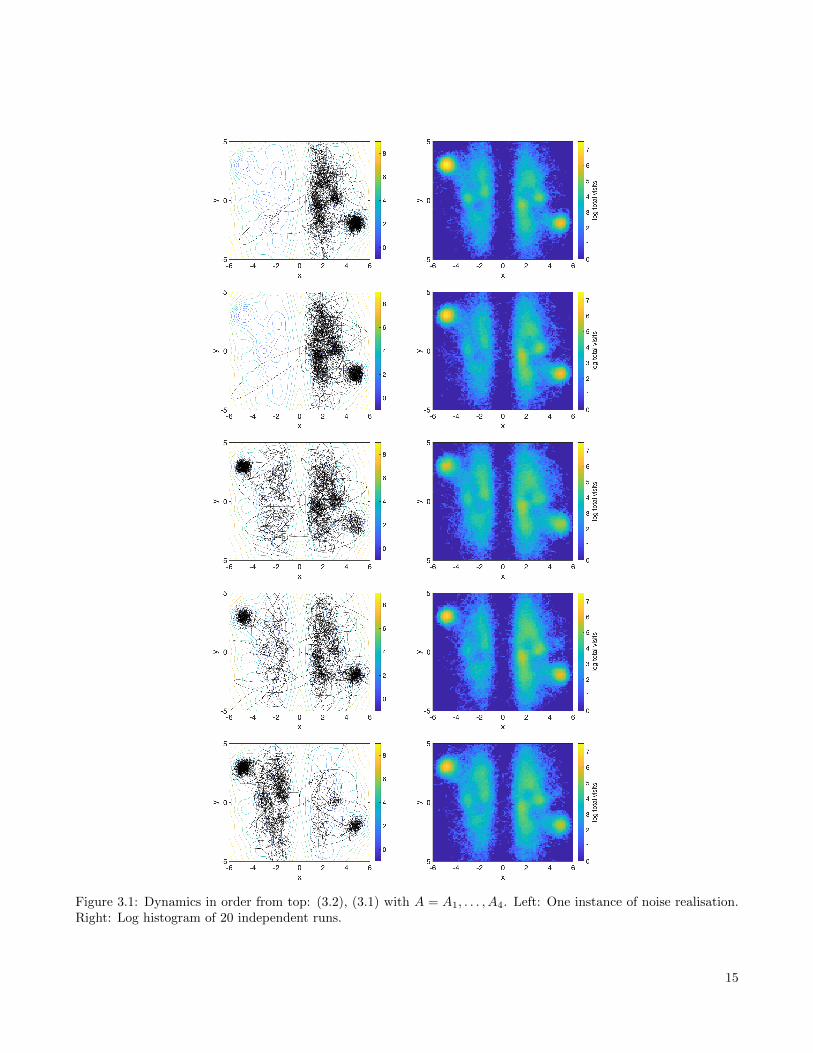
Figure 3.1: Dynamics in order from top: (3.2), (3.1) with A = A1, . . . , A4. Left: One instance of noise realisation.Right: Log histogram of 20 independent runs.

15

Figure 3.2: Proportion of simulations satisfying optimality tolerance for U = U1. Panels from top to bottom:(3.2), (3.1) with A = A1, A2, A3 (A4 is omitted due to numerical instabilities when implementing (3.1)). Left:Final position, right: time-average of last 5000 iterations. We use γ = 3 for improving visualisation, the resultsand improvement in using (3.1) are similar for the case of γ = 1. Results here are for 20 independent runs andk ≤ 5 · 104 -iterations.

16

Figure 3.3: Both proportion of success and numerical transition rates for U = U2. Panels from top to bottom:(3.2), (3.1) with A = A1, A2, A3, A4. Left: Proportion satisfying the optimality tolerance for time-average of last5000 iterations. Right: Average number of crossings across {x1 = 0} for each independent run. The remainingdetails are as in caption of Figure 3.2.

17

Figure 3.4: Results for U = U3. Details are as in caption of Figure 3.3.

18

Appendices

Appendix A Notation and preliminaries

For any φ ∈ C∞ and f : R2n+m → R smooth enough,

Lt(φ(f)) = φ′(f)Lt(f) + φ′′(f)Γt(f), (A.1)

where Γt is the carre du champ operator for Lt given by

Γt(f) =1

2Lt(f

2)− fLt(f) = ∇zf · (A∇zf). (A.2)

The L2(µTt) adjoint L∗t of Lt is

L∗t = − (y · ∇x −∇xU(x) · ∇y)− (z>λ∇y − y>λ>∇z)− T−1t z>A>∇z +A : D2

z .

Recall from Monmarche [47, 48] for Φ : A+ → A, where A and A+ are appropriate spaces (namely A is assumedto be an algebra contained in the domain D(L∗t ) of L∗t fixed by L∗t and A+ = {f ∈ A : f ≥ 0}), differentiable inthe sense that for any f, g ∈ A+,

(dΦ(f).g)(x) := lims→0

(Φ(f + sg))(x)− (Φ(f))(x)

s

exists for all x ∈ R2n+m, the ΓΦ operator for L∗t is defined by

ΓL∗t ,Φ(h) :=1

2(L∗tΦ(h)− dΦ(h).(L∗th)). (A.3)

It will be helpful to keep in mind that L∗t is only a term away from satisfying the standard chain and product rules:

L∗t (ψ(f)) = ψ′(f)L∗t f + ψ′′(f)∇zf · (A∇zf) (A.4)

L∗t (fg) = fL∗t (g) + gL∗t (f) +1

2∇zf · ((A+A>)∇zg) (A.5)

for all f, g ∈ A and ψ ∈ C∞. ∇zf · (A∇zf) and 12∇zf · ((A+ A>)∇zg) are respectively the carre du champ and its

symmetric bilinear operator via polarisation for L∗t .In addition, square brackets on a scalar-valued D1 and a vector-valued operator D2 both acting on scalar-valuedfunctions denote the commutator bracket as follows:

[D1, D2]h = (D1(D2h)1 − (D2D1h)1, . . . ) (A.6)

for h smooth enough; this will be used as in (C.12).

Appendix B Auxiliary results

Proposition B.1. For all t > 0, denote by(XTt , Y Tt , ZTt

)a r.v. with distribution µTt . For any δ, α > 0, there

exists a constant A > 0 such thatP(U(XTt

)> minU + δ

)≤ Ae−

δ−αTt .

Proof. The result follows exactly as in Lemma 3 in [47].

Proposition B.2. Under Assumption 1, for all t > 0, Xt, Yt, Zt are well defined, E[|Xt|2 + |Yt|2 + |Zt|2

]<∞ and

mt ∈ C∞+ = {m ∈ C∞ : m > 0}.

19

Proof. Nonexplosiveness and finiteness of second moments follow as in Proposition 4 in [47] with the modification

G(x, y, t) =1

Tt

(U(x)−min

RnU +

|y|2

+|z|2

).

One can establish that (∂t+Lt)G ≤ CG for some constant C depending on t, Tt. Nonexplosiveness and E[G(Xt, Yt, Zt]] <∞ follow by Markov’s inequality and Ito’s formula, which implies finite second moments for the process.

For smoothness of the law mt of (Xt, Yt, Zt), Theorem 1.2 in [13] can be used.3

For positivity of mt, the steps in Lemma 3.4 of [42] can be followed: for simplicity, consider the case m = n,λ = A = In and Tt = 1, where the associated control problem becomes

Xt + Xt +...Xt +∇U(Xt) +D2

xU(Xt)Xt = Vt, X0 = x0 ∈ Rn (B.1)

where V· : R+ → Rn is a time-varying control and dots indicate partial time derivatives. Given an arbitrary pointX∗ ∈ Rn, set for some fixed T > 0 the control

Vt =

∫ (X∗ − x0

T+∇U

(tX∗ + (T − t)x0

T

)+D2

xU

(tX∗ + (T − t)x0

T

)X∗ − x0

T

)dt.

By the boundedness assumption on the second derivatives of U , the unique solution to the control problem (B.1) is

Xt =tX∗ + (T − t)x0

T. (B.2)

Now since with non-zero probability Brownian motion stays within an ε-neighbourhood of any continuously differ-entiable path, and in particular of Vt, then positivity of mt follows by the support theorem of Stroock and Varadhan(Theorem 5.2 in [63]).For the general case the initial and final values for Y· and Z· are not as above, that is, when Y0 = X0, Z0−∇U(X0) =X0, YT = XT and ZT −∇U(XT ) = XT are arbitrary values. Then it is easy to initialise and finalise Xt and Xt atsome small t > 0 and T − t respectively and extend the previous argument using a piecewise definition of Vt, e.g.see Lemma 4.2 and Appendix of [20].

Appendix C Proof of Proposition 2.3

The following effort up to Proposition C.8 is towards showing dissipation of a distorted entropy as required in theproof of Theorem 2.4.

C.1 Lyapunov function

Lemma C.1. Let δ < 0 be a small enough constant and R : R2n+m+1 → R be defined as

R(x, y, z, Tt) := U(x) +|y|2

2+|z|2

2+ δTt

(y>λ−1z +

1

2x · y

). (C.1)

Then there exist constants a, b, c, d > 0 such that

a(|x|2 + |y|2 + |z|2)− d ≤ R(x, y, z, Tt) ≤ b(|x|2 + |y|2 + |z|2) + d (C.2)

andLt(R) ≤ −cTtR+ d. (C.3)

3This work caters to the unbounded coefficients in the stochastic differential equation, the time-dependence of one of the coefficientsand the need for using the general Hormander’s condition involving the ‘X0’ operator rather than the restrictive one, see [45] fordefinitions. Indeed, the constant assumption 2.(iii) on the annealing schedule for a small interval at the beginning is used so that thistheorem can be applied.

20

Proof. The first statement is clear by the quadratic assumption (2.5) on U for small enough δ. For the secondstatement, fix δ to be small enough for the first statement and additionally to satisfy

δ ≤ Ac2

[(|λ|2

2r1+ 1 +

r2

r1

∣∣λ−1∣∣2)(max

t≥0Tt

)2

+ 2|A|2∣∣λ−1

∣∣2]−1

, (C.4)

where |·| is the operator norm and Ac > 0 is the coercivity constant of the positive definite matrix A.Consider each of the terms of Lt(R) seperately,

Lt

(U(x) +

|y|2

2+|z|2

2

)= − 1

Ttz>Az + TrA. (C.5)

Using the quadratic bound (2.7) on ∇xU ,

Lt(y>λ−1z) = −∇xUλ−1z + |z|2 − |y|2 − T−1

t z>A(λ−1)>y

≤ r1

4r2|∇xU |2 +

r2

r1

∣∣λ−1∣∣2|z|2 + |z|2 − |y|2 +

|y|2

4

+ T−2t |A|

2∣∣λ−1∣∣2|z|2

≤ r1

4|x|2 +

r1

4r2Ug −

3

4|y|2

+

(1 +

r2

r1

∣∣λ−1∣∣2 + T−2

t |A|2∣∣λ−1

∣∣2)|z|2. (C.6)

Then also with the bound (2.6) for ∇xU · x,

Lt(x · y) = |y|2 −∇xU · x+ z>λx

≤ |y|2 − r1|x|2 + Ug +|λ|2

r1|z|2 +

r1

4|x|2. (C.7)

Combining (C.5), (C.6), (C.7), given a large enough C > 0,

Lt(R(x, y, z, Tt)) = Lt

(U(x) +

|y|2

2+|z|2

2

)+ δTtLt(y

>λz) +δTt2Lt(x · y)

≤ −δTtr1

8|x|2 − δTt

1

4|y|2 − 1

Ttz>Az + C

+ δTt

[|λ|2

2r1+

(1 +

r2

r1

∣∣λ−1∣∣2 + T−2

t |A|2∣∣λ−1

∣∣2)]|z|2.Therefore for δ satisfying the bound (C.4), the |z|2 term can be bounded,

Lt(R(x, y, z, Tt)) ≤ −δTtr1

8|x|2 − δTt

1

4|y|2 − Ac

2 maxt≥0 Tt|z|2 + C

≤ −DTtbR+ C ′,

where D > 0 is small enough, C ′ > 0 is large enough and the right inequality of (C.2) has been used.

Lemma C.2. For 2 ≤ p ≤ p with p, p∈N from Assumption 1 on m0, E[R(Xt,Yt,Zt,Tt)p]

(ln(e+t))p is bounded uniformly in time.

Proof. It is equivalent to prove the result for R + d > 0 in place of R for any p ≤ p. Use induction w.r.t. p. Thecase for p = 0 is obvious. Let

Rt := R(Xt, Yt, Zt, Tt).

21

Consider the following terms separately

d

dtE[(Rt + d)p] = ∂tE[(Rt + d)p] + T ′t∂TtE[(Rt + d)p].

Firstly, by definition (C.1) of R and the left bound of (C.2),

T ′t∂TtE[(Rt + d)p] = T ′tE[p(Rt + d)p−1δ

(y>λ−1z +

1

2x · y

)]≤ |T ′t |E

[p(Rt + d)p−1δ

∣∣∣∣y>λ−1z +1

2x · y

∣∣∣∣]≤ Bp

tE[(Rt + d)p]

for a constant Bp ≥ 0.With (A.1) and (A.2), for p ≥ 1, using property (C.3) from Lemma C.1 and again the left bound of (C.2),

consider the auxiliary expression

∂tE[(Rt + d)p] = E[(Lt((R+ d)p))(Xt, Yt, Zt, Tt)]

= E[p(Rt + d)p−1(Lt(R))(Xt, Yt, Zt, Tt))

+ p(p− 1)(Rt + d)p−2(Γt(R))(Xt, Yt, Zt, Tt)]

≤ E[p(Rt + d)p−1(−cTtRt + d)

+ p(p− 1)(Rt + d)p−2(Zt + δTt(λ−1)>Yt) · (A(Zt + δTt(λ

−1)>Yt))]

≤ −cpTtE[(Rt + d)p] +ApE[(Rt + d)p−1]

for a constant Ap ≥ 0. Then with the induction assumption, the slow-decay assumption on Tt, for large enough t,

d

dt(e

c2p

∫ t0TsdsE[(Rt + d)p]) ≤ Ape

c2p

∫ t0Tsds(ln(e+ t))p−1,

E[(Rt + d)p] ≤ E[(R0 + d)p]e−c2p

∫ t0Tsds +

∫ t

0

Ape− c2p

∫ tsTudu(ln(e+ s))p−1ds

≤ E[(R0 + d)p] +Ap(ln(e+ t))p−1

∫ t

0

e−c2pTt(t−s)ds

≤ E[(R0 + d)p] +Ap(ln(e+ t))p−1 1− e− c2pTttc2pTt

.

Using the assumptions on m0 and again the assumption Tt ≥ E(ln t)−1, the result follows.

Corollary C.3. For any 2 ≤ p ≤ p,E[(|Xt|2+|Yt|2+|Zt|2

)p](ln(e+t))p is bounded uniformly in time.

Proof. By the lower bound on R in (C.2),

E[(|Xt|2 + |Yt|2 + |Zt|2

)p] ≤ E[(

R(Xt, Yt, Zt, Tt) + d

a

)p ],

which concludes by Lemma C.2 after expanding.

22

C.2 Form of Distorted Entropy

Let H(t) be the distorted entropy

H(t) :=

∫ (∣∣2∇xht + 8S0(∇yht + λ−1∇zht)∣∣2)

ht+

∣∣∇yht + S1λ−1∇zht

∣∣2ht

+ β(T−1t )ht ln(ht)

)dµTt , (C.8)

where S0, S1 > 0 are the constants

S0 := (1 + |D2xU |2∞)

12 , (C.9)

S1 := 2 + 156S20 + 1024S4

0 (C.10)

and β is a second order polynomial

β(T−1t ) := 1 + β0 + β1T

−1t + β2T

−2t (C.11)

with large enough coefficients β0, β1, β2 > 0 depending on |D2xU |∞,

∣∣A>∣∣ and

λ2 := max(|λ|2,

∣∣λ>∣∣2, ∣∣λ−1∣∣2, ∣∣λ−1

∣∣∣∣λ>∣∣).Remark C.1. This particular expression for H is not necessarily the best choice and it is quite possible to have only∇x and ∇y and no ∇z appearing in the first integrand for instance. However the above is a working expression andoptimality of this is left as future work.

First, an auxiliary result which can be found as Lemma 12 of [47] is stated along with its proofs from [47] sincethe proof is not too long. Notice the Φ∗ appearing in Lemma C.4 appears in the first two terms of H(t).

Lemma C.4. For

Φ∗(h) =|M∇h|2

h,

where M is matrix-valued, we have

ΓL∗t ,Φ∗(h) ≥ (M∇h) · [L∗t ,M∇]h

h

for all 0 < h ∈ A+, where the square bracket denotes the commutator vector (A.6), i.e.

[L∗t ,M∇]h = (L∗t (M∇h)1 − (M∇L∗th)1, . . . ). (C.12)

Proof. The second term in definition (A.3) of ΓL∗t ,Φ(h) can be calculated to be

−dΦ∗(h).L∗th = − 2

h(M∇h) · (M∇L∗th) +

L∗th

h2|M∇h|2. (C.13)

Using the adjusted product and chain rules (A.5) and (A.4) for L∗t , the first term in the definition (A.3) of ΓL∗t ,Φcan be calculated to be

L∗t (Φ∗(h)) =

1

hL∗t (|M∇h|

2) + |M∇h|2L∗t

(1

h

)−∑i

2

h2(M∇h)i∇zh · ((A+A>)∇z(M∇h)i)

=2

h

((M∇h)·L∗tM∇h+

∑i

∇z(M∇h)i · (A∇z(M∇h)i)

)+ |M∇h|2L∗t

(1

h

)−∑i

2

h2(M∇h)i∇zh · ((A+A>)∇z(M∇h)i),

23

where the last summands can be bounded below with the positive definite property of A,

− 2

h2(M∇h)i∇zh · ((A+A>)∇z(M∇h)i)

= − 2

h2(M∇h)i(∇zh)>A(∇z(M∇h)i)−

1

h2(∇z(M∇h)i)

>A((M∇h)i∇zh)

≥ − 2

h3(M∇h)2

i (∇zh)>A∇zh−2

h(∇z(M∇h)i)

>A∇z(M∇h)i,

which produces the bound

L∗t (Φ∗(h)) ≥ 2

h(M∇h)·L∗tM∇h+ |M∇h|2L∗t

(1

h

)− 2

h3|M∇h|2∇zh · (A∇zh).

Combining this with (C.13) then using the adjusted chain rule (A.4),

ΓL∗t ,Φ∗(h) ≥ 1

h(M∇h) · [L∗t ,M∇]h+

1

2|M∇h|2

(L∗t

(1

h

)+L∗th

h2

)− 1

h3|M∇h|2∇zh · (A∇zh)

=1

h(M∇h) · [L∗t ,M∇]h.

With Lemma C.4, the distorted entropy (C.8) can be shown to be a correct one with the following proposition.

Proposition C.5. Let ΨTt be the operator appearing in the integrand of the distorted entropy H, that is

ΨTt(h) :=

∣∣2∇xh+ 8S0(∇yh+ λ−1∇zh)∣∣2

h+

∣∣∇yh+ S1λ−1∇zh

∣∣2h

+ β(T−1t )h ln(h)

for h ∈ A+. It holds that

ΓL∗t ,ΨTt (h) ≥ |∇h|2

h. (C.14)

Remark C.2. H satisfying this property is crucial for proving dissipation in Proposition C.8 and was the mainconsideration when making remark C.1.

Proof. Let Φ1,Φ2,Φ3 be defined byΨTt =: Φ1 + Φ2 + β(T−1

t )Φ3.

Note that the ΓΦ operator is linear in the second operator argument by linearity of L∗t , so that (C.14) is

ΓL∗t ,Φ1(h) + ΓL∗t ,Φ2

(h) + β(T−1t )ΓL∗t ,Φ3

(h) ≥ |∇h|2

h.

Consider ΓL∗t ,Φ3first. Using the definition (A.3) of ΓL∗t ,Φ and the product and chain rule (A.5) and (A.4) for L∗t ,

ΓL∗t ,Φ3(h) =

1

2

(lnhL∗th+ hL∗t lnh+

2|∇zh|2

h− (1 + lnh)L∗th

)=

1

2

(lnhL∗th+ L∗th+

|∇zh|2

h− (1 + lnh)L∗th

)=|∇zh|2

2h. (C.15)

24

Since the goal is to show (C.14), the availability of the term (C.15) means that regardless of how negative of acontribution ΓL∗t ,Φ1

and ΓL∗t ,Φ2makes in the z-derivative term in (C.15), it is not a concern; this is reflected in the

factor β.For ΓL∗t ,Φ1 and ΓL∗t ,Φ2 we use S0, S1 > 0 defined as before in (C.9)-(C.10).

Lemma C.4 gives

hΓL∗t ,Φ1(h) ≥ (2∇x + 8S0(∇y + λ−1∇z))h · [L∗t , 2∇x + 8S0(∇y + λ−1∇z)]h= (2∇x + 8S0(∇y + λ−1∇z))h · (−2(D2

xU)∇y + 8S0(∇x − λ>∇z+∇y + T−1

t λ−1A>∇z)h

= 16S0|∇xh|2 + 2∇xh · ((−2D2xU + 8S0)∇yh)

+∇xh · (8S0(−λ> + T−1t λ−1A>)∇zh) + 64S2

0∇xh · ∇yh+ 8S0∇yh · ((−2D2

xU + 8S0)∇yh)

+ 8S0∇yh · (8S0(−λ> + T−1t λ−1A>)∇zh) + 64S2

0∇xh · (λ−1∇zh)

+ ((−2D2xU + 8S0)∇yh) · (8S0λ

−1∇zh)

+ 8S0(λ−1∇zh) · (8S0(−λ> + T−1t λ−1A>)∇zh).

In order to get a bound in terms of (∂ih)2 terms rather than ∂ih∂jh terms, bounding ∂ih∂jh terms with some careand using the boundedness assumption (2.4) on the second derivatives of U yield

hΓL∗t ,Φ1(h) ≥ 16S0|∇xh|2−(

2|∇xh|2 + 2|D2xU |2∞|∇yh|

2+ 8|∇xh|2 + 8S2

0 |∇yh|2)

−(

2|∇xh|2 + 8S20 λ

2(

1 + T−2t

∣∣A>∣∣2)|∇zh|2)−(|∇xh|2 + 1024S4

0 |∇yh|2)−(

16S0|D2xU |∞|∇yh|

2

+ 64S20 |∇yh|

2)−(

32S20 |∇yh|

2+ 32S2

0 λ2(1 + T−2

t

∣∣A>∣∣2)|∇zh|2)−(|∇xh|2 + 1024S2

0 λ2|∇zh|2

)−((

2|D2xU |2∞ + 32S2

0

)|∇yh|2

+ 32S20 λ

2|∇zh|2)− 64S2

0 λ2(

1 + T−2t

∣∣A>∣∣2)|∇zh|2≥ 2|∇xh|2 + S2

0(−156− 1024S20)|∇yh|2

+ S20 λ

2(− 1160− 104T−2

t

∣∣A>∣∣2)|∇zh|2.ΓL∗t ,Φ2

compensates for the negative y derivatives:

hΓL∗t ,Φ2(h) ≥ (∇y + S1λ−1∇z)h · [L∗t ,∇y + S1λ

−1∇z]h= (∇y + S1λ

−1∇z)h · (∇x − λ>∇z + S1∇y + S1T−1t λ−1A>∇z)h

= ∇xh ·∇yh−∇yh · (λ>∇zh) + S1|∇yh|2+ S1T−1t ∇yh · (λ−1A>∇zh)

+ S1∇xh · (λ−1∇zh)− S1(λ−1∇zh) · (λ>∇zh)

+ S21∇yh · (λ−1∇zh) + S2

1T−1t (λ−1∇zh) · (λ−1A>∇zh),

25

where using the inequalities

∇xh ·∇yh ≥ −1

2|∇xh|2 −

1

2|∇yh|2

−∇yh · (λ>∇zh) ≥ −1

6|∇yh|2 −

3

2

∣∣λ>∣∣2|∇zh|2S1T

−1t ∇yh · (λ−1A>∇zh) ≥ −1

6|∇yh|2 −

3

2S2

1T−2t

∣∣λ−1∣∣2∣∣A>∣∣2|∇zh|2

S1∇xh · (λ−1∇zh) ≥ −1

2|∇xh|2 −

1

2S2

1

∣∣λ−1∣∣2|∇zh|2

S21∇yh · (λ−1∇zh) ≥ −1

6|∇yh|2 −

3

2S4

1

∣∣λ−1∣∣2

gives the bound

hΓL∗t ,Φ2(h) ≥ −|∇xh|2 + (1 + 156S2

0 + 1024S20)|∇yh|2 −

1

2λ2(

3 + S1 + S21

+ 3S41 + S2

1T−1t

∣∣A>∣∣+ 3S21T−2t

∣∣A>∣∣2)|∇zh|2.Putting together the bounds gives (C.14) given the coefficents (C.11) in β are large enough.

C.3 Log-Sobolev Inequality

Proposition C.6. The distorted entropy (C.8) satisfies

H(ht) ≤ Ct∫|∇ht|2

htdµTt , (C.16)

where

Ct = A∗ + β(T−1t )e(UM−Um)T−1

tTt4

max(

2, a−2m

)(C.17)

for all t > 0 and some constant A∗ > 0 depending on |D2xU |∞ and λ.

Proof. The first two terms in the integrand of H(t) after expanding lead directly to the inequality result for A∗.For the last term of H(t), the standard log-Sobolev inequality for a Gaussian measure [29] alongside the propertiesthat log-Sobolev inequalities tensorises and are stable under perturbations, which can be found as Theorem 4.4and Property 4.6 in [30] respectively, yields the result. Since the proof of Property 4.6 in [30] is not too long, it isrepeated for U satisfying the quadratic assumption (2.5) in order to get the precise form of Ct:∫

ht lnhtdµTt =

∫(ht lnht − ht + 1)dµTt

≤∫

(ht lnht − ht + 1)Z−1Tte−

UmTt e−

1Tt

(|a◦x|2+

|y|22 +

|z|22

)dxdydz

= e−UmTt Z−1

Tt

∫ht lnhte

− 1Tt

(|a◦x|2+

|y|22 +

|z|22

)dxdydz

≤ e−UmTt max

(Tt2,max

i

Tt4a2i

)Z−1Tt

∫|∇ht|2

hte−

1Tt

(|a◦x|2+

|y|22 +

|z|22

)dxdydz

≤ eUM−Um

Tt max

(Tt2,Tt

4a2m

)∫|∇ht|2

htdµTt ,

where the first inequality follows by (2.5) since x lnx− x+ 1 ≥ 0 for all x ≥ 0.

26

C.4 Proof of Dissipation

To see that H(t) dissipates over time, it will helpful to be able to pass a time derivative under the integral sign inH(t), which would be straightforward for compactly supported smooth integrands but is not so for H(t). LemmaC.7 constructs compactly supported functions that when multiplied with the integrand in H(t) gives sufficientproperties for retrieving a bound on ∂tH(t) after passing the derviative under the integral sign.

The key nontrivial sufficient property turns out to be (C.18) below.Let ϕ : R→ R be the mollifier

ϕ(x) :=

e1

x2−1

(∫ 1

−1e

1y2−1 dy

)−1

if − 1 < x ≤ 1

0 otherwise,

ϕm(x) :=1

mϕ

(x

m

)and

νm := ϕm ∗ 1(−∞,m2] ≤ 1

for m > 0 where 1(−∞,m2] is the indicator function on (−∞,m2].

Lemma C.7. The smooth functions ηm : R2n+m+1 → Rn

ηm = νm(ln(R+ 2d)),

where d > 0 is the negative of the lower bound of R as in (C.2),

1. are compactly supported,

2. converge to 1 pointwise,

3. satisfy for some constant C > 0 independent of m and t

Ltηm ≤C

m. (C.18)

Remark C.3. Lemma C.7 is different to Lemma 16 in [47]. We believe the few first equations in the proof of Lemma16 [47] is incorrect and contradicts with equation (4) in the same paper. As a result we require proving (C.18)instead of Lemma 17 of [47].

Proof. By the quadratic assumption (2.5) on U and the bound (C.2) on R, R grows quadratically and in particularis bounded below by an arbitrarily large constant at infinity; along with the support of νm being bounded above,the first statement is clear. The second statement is also easy to check.With the chain rule (A.1) and (A.2) for Lt,

Ltηm = ν′m(ln(R+ 2d))Lt ln(R+ 2d) + ν′′m(ln(R+ 2d))(∇z ln(R+ 2d))>A∇z ln(R+ 2d).

It can be seen that ν′m and ν′′m are of at most order m−1, explicitly:

νm(x) =

∫ m2

−∞ϕm(x− y)dy =

∫ x+m2

−∞ϕm(z)dz,

ν′m(x) = ϕm(x+m2) ≤ m−1 maxϕ,

ν′′m(x) = ϕ′m(x+m2) ≤ m−2 maxϕ′.

Therefore for a constant C > 0,

Ltηm ≤ C(m−1Lt ln(R+ 2d) +m−2(∇z ln(R+ 2d))>A∇z ln(R+ 2d)

).

27

A quick calculation using the Lyapunov property (C.3) of R and again the chain rule (A.1) and (A.2) for Lt reveals

Lt ln(R+ 2d) =LtR

R+ 2d− (∇zR)>A∇zR

(R+ 2d)2

≤ −cTtR+ d

R+ 2d− Ac|∇zR|2

(R+ 2d)2

≤ −cTt(R+ d) + cTtd+ d

R+ 2d− Ac|∇zR|2

(R+ 2d)2

(∇z ln(R+ 2d))>A∇z ln(R+ 2d) ≤ |A||∇z ln(R+ 2d)|2

= |A|∣∣∣∣ ∇zRR+ 2d

∣∣∣∣2,which are bounded over R2n+m+1 considering R grows quadratically in space.

The proof of Proposition C.8 follows very closely to Lemma 19 of [47] and its preceding lemmas.

Remark C.4. As explained in Remark C.3, Lemma C.7 uses a different smooth compact function for the truncationthan the one found in Section 5.2 in [47]. Lemma C.7 is designed to establish (C.21) below, which is pivotal for theproof.

Proposition C.8. For any α > 0, there exists some constant B > 0 and some tH > 0 both depending on |D2xU |∞,

A, λ, Tt, α, UM , Um,Ug, E, r2 and am, such that for all t > tH ,

H(t) ≤ B(

1

t

)1−UM−UmE −2α

. (C.19)

Proof. Consider the auxiliary distorted entropies

Hηm(t) =

∫ηm

(∣∣2∇xht + 8S0(∇yht + λ−1∇zht)∣∣2

ht+

∣∣∇yht + S1λ−1∇zht

∣∣2ht

+ β(T−1t )ht ln(ht)

)dµTt

=

∫ηm(Φ1(ht) + Φ2(ht) + β(T−1

t )Φ3(ht))dµTt =

∫ηmΨTt(ht)dµTt ,

where recall ht = mtµ−1Tt

is the ratio (2.3) between the law of the process and its instantaneous equilibrium. Thepoint of Lemma C.7 was so that a time derivative can be pushed under the integral:

d

dtHηm(t) =

∫ηm∂t(ΨTt(ht))dµTt + T ′t

∫ηm∂Tt(ΨTt(ht)µTt)dxdydz, (C.20)

where ∂t is fixed with respect to Tt and vice versa for ∂Tt .Consider the terms separately. Since mt is the law of the process (1.3) and L∗t is the L2(µTt) adjoint of Lt,∫

f∂tmt =

∫fLTt mt =

∫Ltfmt =

∫Ltf

mt

µTtµTt =

∫fL∗t

(mt

µTt

)µTt ,

where LTt is the L2(R2n+m) adjoint of Lt, yielding ∂tmt = L∗thtµTt . This allows the first term in (C.20) to be

28

bounded as follows.∫ηm∂t(ΨTt(ht))dµTt =

∫ηmdΨTt(ht).∂thtdµTt

=

∫ηmdΨTt(ht).

∂tmt

µTtdµTt

=

∫ηmdΨTt(ht).L

∗thtdµTt

= −∫ηm2ΓL∗t ,ΨTt (ht)dµTt +

∫ηmL

∗t (ΨTt(ht))dµTt

= −∫ηm2ΓL∗t ,ΨTt (ht)dµTt

+

∫Ltηm

(ΨTt(ht) + β(T−1

t )e−1)dµTt

≤ −2

∫ηm|∇ht|2

htdµTt+

C

m

∫ (ΨTt(ht)+β(T−1

t )e−1)dµTt (C.21)

by Proposition C.5 and Lemma C.7 where β(T−1t )e−1 is added to force

β(T−1t )(ht lnht + e−1) ≥ 0 =⇒ ΨTt(ht) + β(T−1

t )e−1 ≥ 0.

(C.21) is a satisfactory bound for now - after taking the limit m→∞, the log-Sobolev inequality (C.16) will boundthe first term on the right hand side of (C.21) such that a Gronwall-type argument can be applied.

For the second term in (C.20), consider the Φ1 and Φ2 terms in the integrand ηm∂Tt(ΨTtµTt) = ηm∂Tt((Φ1 + Φ2 +β(T−1

t )Φ3)µTt) of Hηm(t) as

ηm∂Tt(Φi(ht)µTt) = ηm∂Tt

∣∣∣∣Mi∇ ln

(mt

µTt

)∣∣∣∣2mt, i = 1, 2

for the corresponding matrices M1 and M2. With the form (2.2) of the equilibrium µTt , this yields

ηm∂Tt(Φi(ht)µTt) = −2ηm(Mi∇ lnht ·Mi∇∂Tt lnµTt)mt, (C.22)

where the trickiest part, using ZTt =∫R2n+m e

− 1Tt

(U(x)+

|y|22 +

|z|22

)dxdydz, gives

∂Tt lnµTt

= µ−1Tt∂Tt

(Z−1Tte−

1Tt

(U(x)+

|y|22 +

|z|22

))= µ−1

Tt

(− Z−2

Tt∂TtZTt −

Z−1Tt

T 2t

(U(x) +

|y|2

2+|z|2

2

))e−

1Tt

(U(x)+

|y|22 +

|z|22

)

= µ−1Tt

(− µTtZ−1

Tt∂TtZTt −

µTtT 2t

(U(x) +

|y|2

2+|z|2

2

))

=

∫R2n+m

1

T 2t

(U(x) +

|y|2

2+|z|2

2

)dµTt −

1

T 2t

(U(x) +

|y|2

2+|z|2

2

). (C.23)

Integrating by parts in each of the variables x, y, z, where for the x variable ∇xU(x) · x is used, after some manipu-lation using the quadratic assumptions (2.5) and (2.6) for U(x):

p1

(T−1t

)≤ ∂Tt lnµTt +

1

T 2t

(U(x) +

|y|2

2+|z|2

2− n+m

2Tt

)≤ p2

(T−1t

). (C.24)

29

where p1(x) =2a2mnr2+1 x−

(a2mUgr2+1 +Um

)x2 and p2(x) =

a2Mnr1x+

(a2MUgr1

+UM

)x2 are found from bounding the integral

over U(x).Substituting (C.23) back into (C.22),

ηm∂Tt(Φi(ht)µTt) ≤ ηm

(|Mi∇ lnht|2 + T−4

t

∣∣∣∣∣Mi∇(U(x) +

|y|2

2+|z|2

2

)∣∣∣∣∣2)mt

≤ Φi(ht)µTt + CT−4t

(1 + |x|2 + |y|2 + |z|2

)mt (C.25)

for constant C ≥ 0 by the quadratic assumption (2.7) on |∇xU |2 and ηm ≤ 1.

In the second term of (C.20), Φ3(ht) = mtµTt

ln mtµTt

, using the left inequality of (C.24), gives

ηm∂Tt(β(T−1t )Φ3(ht)µTt)

= −ηmT−2t β′(T−1

t )Φ3(ht)µTt − ηmβ(T−1t )∂Tt lnµTtmt

= −ηmT−2t β′(T−1

t )(Φ3(ht) + e−1)µTt + ηmT−2t β′(T−1

t )e−1µTt

− ηmβ(T−1t )∂Tt lnµTtmt

≤ T−2t β′(T−1

t )e−1µTt

+ β(T−1t )

∣∣∣∣∣ p1

(T−1t

)+

1

T 2t

(n+m

2Tt− UM− |a ◦ x|2−

|y|2

2− |z|

2

2

)∣∣∣∣∣mt, (C.26)

where in the last step ηm ≤ 1 and (2.5) have been used.

Putting together the bounds (C.25) and (C.26) and applying Corollary C.3 yields∫ηm∂Tt(ΨTt(ht)µTt)dxdydz ≤ q

(T−1t

)(H(t) + E

[1 + |Xt|2 + |Yt|2 + |Zt|2

])≤ p(T−1t

)(H(t) + C

), (C.27)

where p and q are some finite order polynomial with nonnegative coefficients and C ≥ 0.

Returning to (C.20), collecting (C.21) and (C.27) then integrating from any s to t gives

Hηm(t)−Hηm(s) ≤∫ t

s

(− 2

∫ηm|∇hu|2

hudµTu + |T ′u|p

(T−1u

)(H(u) + C

))du

+O(m−1).

After taking m→∞ then applying Fatou’s lemma for the first terms of both sides and ηm ≤ 1 for the second termon the left, this becomes

H(t)−H(s) ≤∫ t

s

− 2

∫|∇hu|2

hudµTudu+

∫ t

s

|T ′u|p(T−1u

)(H(u) + C

)du (C.28)

≤∫ t

s

((|T ′u|p

(T−1u

)− 2C−1

u

)H(u) + C|T ′u|p

(T−1u

))du, (C.29)

where the last inequality follows by the log-Sobolev inequality (C.16).Taking s→ t, the derivative of H can be seen to be bounded in such a way that Theorem 2.17 of [66] can be appliedto see that

H(t) <∞ ∀t ≥ 0. (C.30)

30

After taking s→ t, it remains to show that

2C−1t � |T ′t |p

(T−1t

)(C.31)

for large t.Here the assumptions on Tt are imposed. Considering the form (C.17) of Ct and that tα � (ln t)p for any p > 0and α > 0 given large enough t, this yields that for any α > 0, there exists t1 > 0 and ci > 0, i = 1, 2, 3 such thatfor all t ≥ t1,

d

dtH(t) ≤

(c1

(1

t

)1−α

− c2(

1

t

)UM−UmE +α

)H(t) + c3

(1

t

)1−α

.

Since E > UM −Um by assumption, taking α small enough, there exists c4 > 0 and t2 > 0 such that for all t ≥ t2,

d

dtH(t) ≤ −c4H(t)

(1

t

)UM−UmE +α

+ c3

(1

t

)1−α

. (C.32)

Setting

γ1(t) := c4

(1

t

)UM−UmE +α

, γ2(t) := c3

(1

t

)1−α

and following the argument as per [47] from Lemma 6 in [46], (C.32) becomes

d

dt

(H(t) e

∫ tt2γ1(s)ds

)≤ e

∫ tt2γ1(s)ds

γ2(t) =γ2(t)

γ1(t)γ1(t)e

∫ tt2γ1(s)ds

, (C.33)

but for any t ≥ t2 and t∗ ≤ t, taking α ≤ 12

(1− UM−Um

E

),

γ2(t)

γ1(t)=c3c4

(1

t

)1−UM−UmE −2α

≤ c3c4

(1

t∗

)1−UM−UmE −2α

, (C.34)

which allows (C.33) to give

H(t) ≤ H(t2)e−

∫ tt2γ1(s)ds

+c3c4

(1

t∗

)1−UM−UmE −2α

(1− e−∫ tt2γ1(s)ds

).

The proof is finished after substituting back in t∗ = t since H(t2) is finite due to (C.30) and the expression

∫ t

t2

γ1(s)ds = c5

((1

t

)−1+UM−Um

E +α

−(

1

t2

)−1+UM−Um

E +α),

grows to infinity as t→∞, where c5 > 0 is a constant.

Remark C.5. The annealing schedule Tt is chosen to satisfy the relationship (C.31) between C−1t and |T ′t |p

(T−1t

).

(C.31) has two purposes - for the coefficient of H(u) on the right hand side of (C.29) to be negative and for thiscoefficient to be much stronger in magnitude for large t than the last term in (C.29). These allow (C.34) andconsequently for (C.33) to be a fruitful step.

Appendix D Additional Results

We conclude the appendices by presenting the analog of Proposition C.8 for the Tt = T > 0 sampling case and aresult about the choice of the annealing schedule.

31

Proposition D.1. Let 1. and 3. of Assumption 1 hold and let Tt = T for all t for some constant T > 0. It holdsthat ∫

|ht − 1|dµT ≤

√2H(0)

β(T )e−

C−1∗2 t

where C∗ is the log-Sobolev constant

C∗ = A∗ + β(T−1)e(UM−Um)T−1 T

4max

(2, a−2

m

). (D.1)

Proof. After Pinsker’s inequality (2.9) and consideration of the definition (C.8) of H, what remains is the partialtime derivative part of the proof of Proposition C.8. The proof concludes by the same calculations, keeping in mindT ′t = 0, until (C.29) followed by the Gronwall argument.

Proposition D.2. The schedule Tt = Eln(e+t) , E > UM − Um is optimal in the sense that for any differentiable

f : R+ → R+, if

Tt =1

f(t)

(UM − Umln(e+ t)

), (D.2)

Ct is the log-Sobolev factor (C.17) and p is the polynomial with nonnegative coefficients from the proof of PropositionC.8, then the relation (C.31):

2C−1t � |T ′t |p

(T−1t

)holds for large times only if lim supt→∞ f(t) ≤ 1.

Proof. Suppose there exists a constant δ > 0 and times (ti)i∈N such that 0 < ti →∞ and

f(ti) ≥ 1 + δ ∀i.

From its definition (C.17),

C−1t ∼ O(e−(UM−Um)T−1

t T−1t ),

which after substituting in the form (D.2) for Tt is

e−(UM−Um)T−1t T−1

t = (e+ t)−f(t) f(t) ln(e+ t)

UM − Um∼ O(t−f(t)f(t) ln t). (D.3)

Compare this to

|T ′t |p(T−1t

)∝ p(f(t) ln(e+ t))

(f(t) ln(e+ t))2

(f(t)

e+ t+ |f ′(t)| ln(e+ t)

), (D.4)

which has order at least (tf(t))−1(ln t)−2. For t = ti large enough, f(t) ≥ 1 + δ and so

t−f(t)f(t) ln t� (tf(t))−1(ln t)−2, (D.5)

violating (C.31).

Remark D.1. One can strengthen the proposition by making precise the form of p from Proposition C.8, whichwill determine how slowly f(t) is allowed to converge to 1; in fact p should be at least fifth order. This appearsinconsequential with respect to optimality and so is omitted.

32