on the estimation of ocean engineering design contoursjonathan/2014_jntewnfln_dsgcnt_jomae.pdf ·...
TRANSCRIPT

On the estimation of ocean engineering designcontours
Philip JonathanShell Technology Centre Thornton
P.O. Box 1Chester
United [email protected]
Kevin EwansSarawak Shell Bhd
eTiQa Twins (Level 23, Tower 1)50450 Kuala Lumpur
Jan FlynnShell International Exploration and Production
P.O. Box 602280 AB RijswijkThe Netherlands
Accepted for Journal of Offshore Mechanics and Arctic Engineering, June 2014
ABSTRACTUnderstanding extreme ocean environments and their interaction with fixed and floating structures is critical for
offshore and coastal design. Design contours are useful to describe the joint behaviour of environmental, structuralloading and response variables. We compare different forms of design contours, using theory and simulation,and present a new method for joint estimation of contours of constant exceedance probability for a general setof variables. The method is based on a conditional extremes model from the statistics literature, motivated byasymptotic considerations. We simulate under the conditional extremes model to estimate contours of constantexceedance probability. We also use the estimated conditional extremes model to estimate other forms of designcontours, including those based on the First Order Reliability Method, without needing to specify the functionalforms of conditional dependence between variables. We demonstrate the application of new method in estimationof contours of constant exceedance probability using measured and hindcast data from the Northern North Sea, theGulf of Mexico and the North West Shelf of Australia, and quantify their uncertainties using a bootstrap analysis.
1 IntroductionWe are interested in joint estimation of design contours for a general set of p variables X = {X j}p
j=1, characterisingthe ocean environment, structural loading and response in offshore design applications. Development of design contoursusing methods related to the First Order Reliability Method (FORM), see, e.g. [1], [2], [3], [4], have proved popular withpractitioners since extreme environments are characterised independently of structural loading and response, in a mannerwhich lends itself to subsequent interpretation in terms of structural loading and response. For example, [5] describe theestimation of inverse-FORM contours for winds, waves and current off West Africa. In such analyses, we suppose it ispossible to transform X into a set of independent random variables, V = {Vj}p
j=1. Using the probability integral transform,we further transform these independently to standard normal random variables U = {U j}p
j=1. This set has a joint probabilitydensity function f (u) = (2π)−p/2 exp(− 1
2‖u‖2) where ‖u‖2 = uT u is the Euclidean norm of u. The surface S(β) defined by
‖u‖= β (a circle in 2-dimensions, p = 2) corresponds to a surface of constant probability density. We select the value of β
such that S(β) encloses a set with given probability of occurrence, for example, or corresponds to a specified return periodmarginally (i.e. along any axis).
Contours of constant probability density are not the only possibilities, however. For example, consider the definitionof a return value in the univariate case. A return value x corresponding to a T -year return period of random variable X isdefined by Pr(X > x) = 1
nT, where nT is the number of events in the period. That is, x is defined in terms of an exceedance
probability. Extending the analogy to two dimensions, the set of points x(θ) = {x j(θ)}2j=1,θ ∈ [0,360) (say), on a contour
of constant exceedance probability α can be defined by the expression:
Pr(2⋂
j=1
(r j(θ;r0)X j > r j(θ;r0)x j(θ))) = α
where r(θ;r0) = {r j(θ;r0)}2j=1 is defined by r(θ;r0) = x(θ)− r0. Here, r0 is a reference location for the distribution
under consideration. In some cases, it is appropriate that r0 refer to some central feature (e.g. mean, median or mode). Inother situations, when we are interested solely in the large values of a variable Xk, k = 1,2, (i.e. in the right hand tail ofits distribution), it is appropriate to set r0k = 0. We might construct the contour in terms of the original variables X, or anytransformation thereof, in particular the independent standard normals U.
A key assumption in the estimation of FORM-type design contours is problem representation in terms of a set of inde-pendent random variables V. Consider the case p = 2. The probability density f (x1,x2) can be factorised as f (x1) f (x2|x1),in principle. In some applications, a model based on V1 = X1 and V2 = X2|X1 = x1 is justified on physical grounds, so thatV are independent. For example, it is common (e.g. [2]) to model the pair of variables significant wave height HS and peakperiod TP in terms of HS (assumed to be Weibull-distributed) and TP|HS = h (assumed to be independently log-normallydistributed). If this model can be shown to fit well throughout the sample, we can estimate contours of constant probabilitydensity. Whereas the model appears to explain the body of sample data well, it is not clear (e.g. [6]) whether this model isappropriate for extremes of HS and TP. The generalised Pareto distribution has a stronger asymptotic motivation for mod-elling (peaks over threshold) of HS than the Weibull. The log-normal parameter estimates (for TP|HS) fitted within the bodyof the sample may not be relevant for extrapolation to extremes. The conditional form V2 = (X2|X1 = x1) will not be knownin general, and might not be easily or adequately approximated.
The conditional extremes model of [7] provides a means to model the marginal and dependence structure of extremes ofthe set X, by (1) (marginal) modelling of threshold exceedances of each variable independently (using the generalised Paretodistribution), (2) (dependence) modelling of pairs Yj|Yk = yk for threshold exceedances of Yk, ( j = 1,2, ..., p, j 6= k;k =1,2, ..., p), following a transformation of variables from the original (X) scale to standard Gumbel (Y ) scale. We estimatecontours of constant exceedance probability by simulation under the model. The conditional extremes model is motivated byasymptotic considerations, and has been reported by the current authors in the past ( [6]). It provides a conditional decom-position of variables, given threshold exceedances of the conditioning variate, which is generally applicable for estimationof design contours. It can complement (or replace) FORM-type analysis when functional forms of conditional relationshipsare not known, and has a strong underpinning in multivariate extreme value theory. It is particularly relevant to estimation ofcontours of constant exceedance probability on the original (X) scale of variables, as will be illustrated below.
The layout of the article is as follows. In Section 2, we introduce four applications motivating the current work. InSection 3, we overview the conditional extremes model and its application in estimation of design contours of differentforms. In Section 4, we evaluate the performance of the conditional extremes model in estimating all design contoursfor a simulated example. In Section 5, we estimate contours of constant exceedance probability for the four applicationsintroduced in Section 2. Conclusions are made in Section 6. The appendix gives a fuller description of the conditionalextremes model.
We note that, for p > 2, the terms surface or manifold would be more appropriate than contour. We persist with the latterfor ease of understanding. Further, in 2 dimensions, we note that the parameter θ ∈ [0,360) used to reference the contour isdefined in the usual mathematical sense, anti-clockwise from the abscissa. Significant wave height (HS) and peak spectralperiod (TP) have units of metres and seconds respectively throughout.
2 DataWe motivate current work by considering applications to estimation of extreme values of HS and TP at a location in the
Northern North Sea (NNS) for which both measured and hindcast data are available, to buoy data from a location in theGulf of Mexico (GoM), and to hindcast data on the North West Shelf (NWS) of Australia. Data correspond to storm peakvalues for HS over threshold, observed during periods of storm events, and corresponding values for TP. For the measuredNNS example, illustrated in Figure 6, the sample corresponds to 620 storm peak pairs for the period (March 1973, December2006) measured using a laser device. Hindcast data for the same NNS location (see Figure 7) corresponds to 827 pairs ofvalues for the period (November 1964, April 1998). GoM data in Figure 8 are National Data Buoy Center measurementsfrom buoy 42002 corresponding to 505 pairs for the period (January 1980, December 2007). Finally, NWS hindcast data(shown in Figure 9) correspond to 145 pairs of storm peak values for the period (February 1970, April 2006). All samplesexhibit positive dependence between HS and TP. The four application data sets are chosen to illustrate methods of estimationof design contours, not for development of design criteria. In general, sample sizes are only of the order of 30 years inlength, and data include strong covariate effects due, for example, to seasonality. No attempt has been made at this point toaccommodate these effects in the analysis.
3 Illustration and evaluation3.1 Conditional extremes model
Here we outline the conditional extremes model in 2 dimensions. A fuller description of the model in p dimensions isgiven in the appendix. For pairs (Y1,Y2) of random variables with marginal Gumbel distributions, [7] derive a parametric

form for the conditional distribution of one variable given a large value of the other. This parametric form, motivated bythe assumption of a particular limit representation for the conditional distribution (see [6]) is appropriate to characterisethe conditional behaviour of a wide range of theoretical examples of bivariate (and higher-dimensional) distributions forextremes. Model form for positively associated pairs of variables (Y1,Y2) takes a particularly simple form:
(Y2|Y1 = y1) = ay1 + yb1Z
where a and b are location and scale parameters respectively to be estimated, with a ∈ [0,1] and b ∈ (−∞,1), and y1is large. Z is a random variable, independent of Y1, converging with increasing y1 to a non-degenerate limiting distributionG. Joint tail behaviour is then characterised by a, b and G. The form of distribution G is not specified by theory. For asample {yi1,yi2}n
i=1 of values from (Y1,Y2) with values of Y1 exceeding an appropriate threshold wY 1, the values of a, b andG are estimated using regression. For simplicity and computational ease during model fitting, G is assumed to be a Gaussiandistribution with mean µZ and variance σ2
Z treated as nuisance parameters. Fitted values:
zi =(yi2− ayi1)
ybi1
, i = 1,2,3, ...,n
are used to estimate distribution G, and the estimate G is then sampled in subsequent simulations. The adequacy of modelfit can be assessed by (1) demonstrating that the values {zi}n
i=1 and {yi1}ni=1 are not obviously dependent, (2) exploring the
effect of varying wY 1 on a, b and subsequent estimates (e.g. of probabilities associated with extreme sets), and (3) bootstrapresampling to estimate the uncertainty of estimates for a, b and subsequent estimates for a given threshold choice.
The generalised Pareto (GP) form is appropriate for model marginal distributions of peaks over threshold, rather than theGumbel distribution. Therefore, in such cases, to use the conditional model above we transform original variables (X1,X2)from GP to Gumbel using the probability integral transform as follows. Suppose we fit the GP distribution (to the samplefrom X1 without loss of generality):
FGP(x1;ξ,β,u) = 1− (1+ ξ
β(x1−u))
− 1ξ
+
and estimate cumulative probabilities {FGP(xi1; ξ, β,u)}ni=1. The standard Gumbel distribution has cumulative distribu-
tion function FG(x) = exp(−exp(−x)), thus if we define the transformed sample {yi1}ni=1 such that FG(yi1) = FGP(xi1; ξ, β,u)
or:
yi1 =− log(− log(FGP(xi1; ξ, β,u))) for i = 1,2,3, ...,n
the transformed sample will be consistent with a sample from a Gumbel distribution. Similarly, given a value y1 (ofGumbel variate), we can calculate the corresponding value x1 on the original GP scale. It is essential to demonstrate theadequacy of GP marginal fits, e.g. by using the mean residual life plot and stability of marginal shape parameter as a functionof threshold choice. Finally, to simulate a random drawing from the conditional distribution Y |X > u, the following procedurecan then be followed: (1) draw a value y1 of Y1 at random from its standard Gumbel distribution, given that the value exceedsthreshold wY 1, (2) draw a value of z of Z at random from the set {zi}n
i=1, (3) calculate that value of y2|y1 = ay1 + yb1z,
(4) transform (y1,y2) to (x1,x2) using the probability integral transform and the estimated GP marginal model parameters.Using simulation, estimates for various extremal statistics (e.g. values associated with long return periods) can be obtainedroutinely. Modelling and simulation of (Y1|Y2 = y2) can be achieved in the same way. Extension to p-dimensional variatesis outlined in the appendix.
3.2 Contours of constant exceedance probabilityContours of constant exceedance probability can be estimated for a general set of variables M = {M j}p
j=1 (e.g. onoriginal (X), independent (V ), independent standard normal (U) or Gumbel (Y ) scales). The contour is defined as the setm(θ) = {m j(θ)}p
j=1,θ ∈ [0,360)p−1 such that:

Pr(p⋂
j=1
(rM j(θ;rM0)M j > rM j(θ;rM0)m j(θ))) = α
where rM(θ;rM0) = {rM j(θ;rM0)}pj=1 is defined by rM(θ;rM0) = m(θ)− rM0, where rM0 is a reference location for the
distribution under consideration. Thus rM(θ;rM0) is the position vector of the contour, as a function of angle θ, relative toreference location rM0, beyond which the probability of non-exceedance is a constant in the sense defined.
We now define four forms of design contour for further consideration.
3.3 Design contour C1: Constant probability density on independent standard normal scaleWe assume that FORM-type models are available to transform the original set of variables X to independent standard
Normal random variables U. Following the description in Section 1, we evaluate the hyper-sphere ‖u‖ = β for which thejoint probability density function f (u) = (2π)−p/2 exp(− 1
2‖u‖2) is a constant. We select the value of β corresponding to a
specific return value of U1. We then back transform the contour to the original (X) scale for interpretation.
3.4 Design contour C2: Constant exceedance probability on independent standard normal scaleAs for contour C1, we assume we can transform the original set of variables X to independent standard Normal random
variables U. We evaluate contours of constant exceedance probability using the equation in Section 3.2 with M = U, with areference location rU0 = 0. We then back-transform the contour to the original (X) scale for interpretation.
In p = 2 dimensions, in the first quadrant (θ ∈ (0,90)), the contour corresponds to Pr(U1 > u1(θ),U2 > u2(θ)) = α. Inthe second, third and fourth quadrants (θ∈ (90,180), θ∈ (180,270) and θ∈ (270,360) respectively), corresponding contourdefinitions are Pr(U1 ≤ u1(θ),U2 > u2(θ)) = α, Pr(U1 ≤ u1(θ),U2 ≤ u2(θ)) = α and Pr(U1 > u1(θ),U2 ≤ u2(θ)) = α.
3.5 Design contour C3: Constant one-sided exceedance probability on independent standard normal scaleThis contour differs from C2 only in the choice of reference location rU0. To achieve a constant one-sided exceedance
contour with respect to any subset XK , K ⊆ { j}pj=1, we set the corresponding components of rU0 to the minimum values of
UK observed in the data sample. Again, we back transform the contour found to the original (X) scale for interpretation.In p = 2 dimensions, in the first and second quadrants (θ ∈ (0,180)), contour definition is Pr(U1 > u1(θ),U2 > u2(θ)) =
α, whereas in the third and fourth quadrants (θ ∈ (180,360)), contour definition is Pr(U1 > u1(θ),U2 ≤ u2(θ)) = α.
3.6 Design contour C4: Constant one-sided exceedance probability on original scaleWe estimate contours using the equation in Section 3.2 with M=X, i.e. using the original variables, by direct simulation
under the conditional extremes model in p dimensions, necessitating the estimation of conditional extremes models withrespect to each of the p variables, as outlined in the appendix. The reference location definition is analogous to that for C3.
In p = 2 dimensions, in the first and second quadrants (θ ∈ (0,180)), the contour definition is Pr(X1 > x1(θ),X2 >x2(θ)) = α, whereas in the third and fourth quadrants (θ∈ (180,360)), the contour definition is Pr(X1 > x1(θ),X2 ≤ x2(θ)) =α.
4 Design contours using the conditional extremes modelWe illustrate the characteristics of the four design contours C1-C4 introduced in Section 3 above, using a 2-dimensional
model for the pair (X1,X2)=(HS,TP) discussed in [8]. We also quantify the performance of the conditional extremes model inapproximating each of these contours. We assume that HS is Weibull-distributed as follows:
FHs(h) = exp(−( h2.822
)1.547)
Conditionally on HS, TP is assumed independently log-normally distributed:
((loge TP)|HS = h) = 1.59+0.42loge(HS +2)
+√
0.005+0.085exp(−0.13H1.34S ) ε

where ε is a standard Normal random variate.
4.1 True model design contoursGiven these functional forms, we can evaluate true contours C1-C4 for any return value. Figure 1 shows the contours
corresponding to a 1 in 1000 event of HS marginally, together with a random sample of 1000 values from the model (forillustration only).
[Fig. 1 about here.]
A number of interesting features can be observed from the figure. The maximum value of HS for each of the contours is thesame by construction (corresponding to the 1 in 1000 event). The constant density contour C1 (dashed black) is continuousand smooth (i.e. continuous first derivative) whereas the constant exceedance probability contours C2-C4 are continuous butnot smooth. Contours C2 (solid grey) and C3 (dashed grey) are identical for values of HS above its median by definition. Forthis example, the locations of the four contours are relatively similar.
[Fig. 2 about here.]
[Fig. 3 about here.]
[Fig. 4 about here.]
[Fig. 5 about here.]
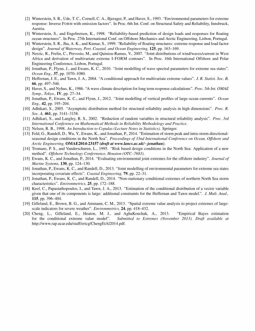
4.2 Design contours estimated using the conditional extremes modelNow we use the conditional extremes model to estimate each of the contours C1-C4 by fitting to a sample. A random
sample of 1000 values was drawn from the HS-TP model and the conditional extremes model estimated using a thresholdcorresponding to the 80%ile used for marginal modelling, and the 95%ile for conditional model. The estimated conditionalextremes model is then used to estimate the four contours C1-C4 in turn. For estimation of C1-C3, only the estimatedconditional extremes model parameters are required for contour estimation. For contour C4, we simulate a sample of 10000values under the conditional extremes model, and estimate the contour empirically (by counting). Results are shown inFigures 2-5 respectively, in terms of estimates for bootstrap median (thick black) and 95% band (thin black) for HS(θ) (solidblack) and TP(θ) (dashed black) on the contour for θ∈ [0,360). Also shown, for each figure, is the corresponding true contour(in grey). The bootstrap analysis is based on full modelling of 100 re-samples of the original data, and quantifies the samplinguncertainty of the whole modelling procedure. We note that, for contours C1-C3, the conditional exceedance model can onlybe used to estimate the section of the contour corresponding to exceedances of the HS threshold, since the conditionalextremes model applies only to extremes of HS and corresponding conditional values of TP. For contour C4, however,simulation under the conditional extremes model allows the full contour to be estimated. We see from the figures thatagreement between true contours and their estimates is good in each case. Moreover, contour estimates from the conditionalextremes model were achieved without explicit knowledge of the HS-TP model. This suggests that the conditional extremesmodel is applicable for evaluation of design contours for arbitrary sets of variables, with no requirement for knowledge ofconditional relationships between variables (other that that provided by the sample data).
[Fig. 6 about here.]
[Fig. 7 about here.]
[Fig. 8 about here.]
[Fig. 9 about here.]
5 ApplicationThe four samples of measured and hindcast (storm peak) HS and TP data selected to illustrate development of design
contours using the conditional extremes model are introduced in Section 2. Marginal and conditional extremes modellingof the samples has been reported in [6]. Threshold selection in marginal modelling was noted to be problematic in somecases. Based on assessment of various diagnostics plots, particularly the variability of marginal and conditional modellingparameters, and marginal return value estimates, with threshold, a 60%ile threshold was adopted for marginal modelling anda 70%ile threshold for conditional modelling in all four cases. Uncertainties in model parameter estimates, quantified usinga bootstrap analysis, has also been reported in [6]. Here, we focus on the estimation of contours of constant exceedanceprobability (of type C4), one-sided with respect to HS, corresponding to return periods of 10, 100 and 1000 years. Figures6-9 show estimates for measured NNS, hindcast NNS, measured GoM and hindcast NWS respectively, together with a scatter
plot of the corresponding samples. All contour estimates are based on a 10,000 year full simulation using the conditionalextremes model. The measured and hindcast NNS contours (for the same nominal location) would appear to be qualitativelysimilar. The spacing of contours corresponding to different return periods is larger for the measured GoM indicates longmarginal tails, particularly in TP. The hindcast NWS contours show a complex structure.
Figures 10-13 show 100 year contour estimates in terms of bootstrap median (thick) and 95% uncertainty band (thin) forHS(θ) (solid) and TP(θ) (dashed), for θ ∈ [0,360). There is considerable uncertainty in the location of the contour, reflectinguncertainties in estimating marginal and dependence model parameters.
[Fig. 10 about here.]
[Fig. 11 about here.]
[Fig. 12 about here.]
[Fig. 13 about here.]
6 Discussion and conclusions[Fig. 14 about here.]
[Fig. 15 about here.]
[Fig. 16 about here.]
[Fig. 17 about here.]
For contours of types C1-C3 (see Section 3), based on an independent standard normal representation, the conditionalextremes model can only provide an estimate for the part of the contour corresponding to large values of HS (for which theconditional extremes model is valid). Nevertheless, in practice, interest in design contours usually focusses on sections ofthe contour corresponding to large values of at least one variable. Figures 14-17 show portions of the conventional FORMcontours C1, estimated using the conditonal extremes model, directly comparable to Figures 10-13, in terms of median andbootstrap 95% uncertainty bands as a function of angle. For contours based on exceedances on the original variable scale(see Section 3.6), some choices of reference location rX0 (e.g. the sample median) will result in contour estimates which arediscontinuous.
A comparison of the HS− TP model and conditional extremes models for joint estimation of extremes of (HS,TP) isgiven in [6]).
Contours of constant exceedance probability estimated using the conditional extremes models (e.g Figures 6-9) are notsmooth in general, since the conditional extremes model simulation is based on a resampling of the set of model residuals{zi}n
i=1 (see Section 3.1 for p = 2), where n is the number of threshold exceedances available for modelling. Increasingsimulation size will not produce smoother contours in general. These could be achieved by fitting a parametric model toresiduals {zi}n
i=1 and sampling from it, at the price of increased modelling complexity and additional modelling uncertaintywhich we have chosen to avoid.
As explained in the appendix, the conditional extremes model can be used to model and simulate from p-dimensionaldistributions, p > 2; [9] use such analysis for joint modelling of extreme current profiles (with p = 32). Contours of constantexceedance probability can be estimated in higher dimensions; computationally, the size of simulations increases with p andin this sense the analysis becomes more complex. To estimate a FORM-type contour in higher dimensions would require thespecification and/or estimation of an increasing number of (usually unknown) conditional distributions. [10] discusses issuesin application of first- and second-order reliability models in higher dimensions.
For 2 independent standard normal variates U1 and U2, it is useful to note that a contour of constant probability densityis defined by pairs of values (u1,u2) satisfying u2
1+u22 = cD, whereas a contour of constant exceedance probability is defined
by expressions (1−Φ(u1))(1−Φ(u2)) = cE , (1−Φ(u1))Φ(u2) = cE , Φ(u1)(1−Φ(u2)) = cE and Φ(u1)Φ(u2) = cE , whereΦ is the cumulative distribution function of the standard normal distribution. cD and cE are a related pair of constants.
A key design objective is the estimation of structural integrity. Given the joint probability density fX(x) of environmentaland structural loading variables, and a failure surface (or limit-state function) g(X), such that the structure failures wheng(X)≤ 0 and is safe otherwise, the failure probability of the structure can be expressed as
∫g(X)≤0 fX(x)dx. In FORM analysis
(see, e.g., [11]), this integral is approximated in terms of a single design point. Assuming that transformation of variablesto independent standard Normals U is possible (see, e.g., contour C1 in 3.3 above), the FORM design point is given byu∗ = arg min(uT u)s.t.g(u) = 0, and the failure probability by Φ(−β), where β= uT u, where Φ is the cumulative distributionfunction of the standard Normal distribution. Using full simulation under the conditional extremes model, direct estimationof failure probability (and its uncertainty) is possible avoiding the need for design points. Were an estimate of probability
density fX(x) required, this could be achieved from the simulation (e.g. by estimating, smoothing and differentiating anempirical copula, [12]).
In practice, the best choice of contour (including C1-C4 and many other possibilities) to employ depends on the re-quirements of the application. Analogy with the univariate definition of return value suggests that contours should be basedon constant one-sided non-exceedance probability (such as C4). Within FORM-type procedures, involving the (often un-justified) assumption of a Gaussian dependence structure, contours of constant non-exceedance probability coincide withthose of constant probability density. The analysis in this paper concentrates on characterising the extremal dependencebetween storm peak events of HS and TP. From a structural risk perspective, particularly for floating structures exhibitingresonant responses to the ocean environment, we note that important combinations of environmental variables might occuraway from the peaks of storms. For this reason, we might choose to include short-term environmental variability and exam-ine extremal dependence structure on a sea-state basis (see, e.g. [13]). Alternatively, we might include structural responsevariables (estimated as in [14], e.g.) within the conditional extremes model.
Bootstrap uncertainty analysis quantifies (sampling) uncertainties associated with model fitting, but cannot estimate theinadequacy of model form (regardless of the model being fitted). Simply stated, we have no reason in general to believe that amodel (such as the HS-TP model above) estimated using the body of a multivariate sample will be appropriate to characteriseits extremes. However, as we move into the tail of the sample away from its body, it is difficult to estimate when exactly thatmodel becomes unreliable. Conversely, the conditional extremes model has a solid foundation in the asymptotic theory ofmultivariate extreme values. However, it is nevertheless difficult to estimate how far into the tail of the data we must venture(with ever reducing sample size for modelling) so that the model becomes sufficiently reliable. These issues becomes morepressing as p increases; the curse of dimensionality. For serious application of the conditional extremes model, carefulassessment of the sensitivity of estimates to fundamentals such as the choice of extreme value threshold (for all marginaland pairwise dependence estimation) and variable scale (for marginal modelling) are crucial. Incorporation of the effectsof covariates such as location, direction, season and time is vital for reliable application of both conditional extremes andFORM-type models.
In this paper, we consider various approaches to the specification of design contours for ocean engineering applications.We illustrate and compare these approaches under known model conditions. We introduce design contours based on theconditional extremes model of [7]. We show that the conditional extremes model can be used to estimate different forms ofdesign contours at least in part, without the need for model form assumptions required for FORM-type analysis. Because ofits asymptotic motivation, the conditional extremes model is likely to give better representations of design contours for jointextremes, compared to contours based on modelling the non-extreme body of the sample. In particular, we show that a fullsimulation under the conditional extremes model can be used to estimate contours of constant exceedance probability for theoriginal variables (of type C4), and quantify the uncertainty with which that contour is estimated. We consider this to be aninteresting supplement to ocean engineering methods.
AcknowledgementsThe authors gratefully acknowledge funding from Shell, and discussions with colleagues at Shell and Lancaster Univer-
sity, UK.
Appendix A: Conditional extremes model in p dimensionsThis section describes the conditional extremes model in p dimensions, extending the outline (for p = 2) in Section 3.1
of the main text. For a vector Y (= {Yj}pj=1) of random variables with marginal Gumbel distributions, [7] derive a parametric
form for the conditional distribution of the remaining variables Y−k (= {Yj}pj=1, j 6=k) given a large value yk of the variable Yk,
at least as large as threshold wY k , k = 1,2, ..., p. The conditional model form for positively dependent variables Y is:
(Y−k|Yk = yk) = akyk + ybkk Zk, where yk > wY k, for k = 1,2, ..., p
where ak (= {a jk}pj=1, j 6=k) and bk (= {b jk}p
j=1, j 6=k) are vectors of location and scale parameters respectively to be esti-mated, with element a jk ∈ [0,1] and b jk ∈ (−∞,1), and yk large, for j = 1,2, ..., p, j 6= k, and k = 1,2, ..., p, and component-wise multiplication is understood (i.e. for p-dimensional vectors r = {ri}p
i=1 and s = {si}pi=1, then rs = {risi}p
i=1). Zk is avector random variable, independent of Yk, converging with increasing yk to a non-degenerate limiting distribution Gk. Foreach k, k = 1,2, ..., p, joint tail behaviour conditional on Yk is characterised by ak, bk and Gk. The form of distribution Gk isnot specified by theory. When two variables Yj,Yk are negatively dependent (i.e. a jk = 0,b jk < 0), the form of the conditionalrelationship is slightly different, but still amenable to empirical modelling:
(Y−k|Yk = yk) = ck−dkloge(yk)+ ybkk Zk, where yk > wY k
for k = 1,2, ..., p, where ck (= {c jk}pj=1, j 6=k) and dk (= {d jk}p
j=1, j 6=k) have elements such that c jk ∈ (−∞,∞) and d jk ∈[0,1]. For a sample {yi j}n,p
i=1, j=1 of values from Y with values of conditioning variate Yk exceeding an appropriate thresholdwY k, the values of ak, bk and Gk are estimated using regression. For simplicity and computational ease during model fitting,Gk is assumed to be a multivariate normal distribution with mean µZk and diagonal variance-covariance matrix with elementsσ2
Zk treated as nuisance parameters, for k = 1,2, ..., p. These assumptions resolve the modelling procedure into fitting ofp− 1 pairwise models for pairs (Yj,Yk), j = 1,2, ..., p, j 6= k, for each of p conditioning variates Yk, k = 1,2, ..., p. Fittedresiduals:
zi jk =(yi j− a jkyik)
yb jkik
, i = 1,2,3, ...,n, j,k = 1,2, ..., p, j 6= k
provide a dependent sample from the multivariate distribution Gk, which is then resampled (with replacement) in subse-quent simulations. The adequacy of model fit can be assessed by (1) demonstrating that the values {zi jk}n
i=1 and {yik}ni=1 are
not obviously dependent, (2) exploring the effect of varying wY k on a jk, b jk and subsequent estimates (e.g. of probabilitiesassociated with extreme sets), and (3) bootstrap resampling to estimate the uncertainty of estimates for ak, bk and subsequentestimates for a given threshold choice wY k (see e.g. [6]).
Marginal modelling of the original data (in terms of variables X (= {X j}pj=1)) proceeds independently per variable as
described in the main text, as does transformation between original and Gumbel variates.
Conditional simulationTo simulate a random drawing {xs j}p
j=1 from the conditional distribution X−k|Xk > wXk, the following procedure canthen be followed:
1. draw a value ysk of Yk at random from the standard Gumbel distribution,2. draw a set of values {zs jk}p
j=1, j 6=k of Z−k at random from the set {zi jk}n,pi=1, j=1, j 6=k generated during model fitting,
3. calculate that value of ys j|ysk = a jkysk + yb jksk zs jk for j = 1,2, ..., p, j 6= k,
4. transform {ys j}pj=1 to {xs j}p
j=1 using the probability integral transform and the estimated GP marginal model parameters.
To use this scheme to generate a multivariate dependent sample, we must first estimate the relative frequency with which tocondition on each variable Yk (or Xk), k = 1,2, ..., p, in turn. This is achieved as follows. Note that the sample {yi j}n,p
i=1, j=1corresponds to a subset E of the original sample, for which the value of at least one variable (for each observation) exceedsits corresponding threshold (wY k for variable k). We can therefore partition E into the union of sets {Ek}p
k=1:
Ek = {{yi j}n,pi=1, j=1 s.t. yik > yi j; j = 1,2, ..., p, j 6= k; i = 1,2, ...,n}
so that for observations in set Ek, the value of variable k is more extreme in its marginal distribution than the value ofany other variable. Since the conditional extremes model is motivated asymptotically, it is most appropriately applied to theconditioning variate whose value is most extreme in its distribution. We therefore use the relative frequency of observations inthe sets {Ek}p
k=1 to determine the rate at which we condition on each variable Yk, k = 1,2, ..., p, during conditional simulation.See [7] for further discussion.
A number of applications and extensions of the conditional extremes approach have been reported. [15] discuss theevaluation of environmental joint extremes for the offshore industry, including the incorporation of covariates (such as stormdirection) within the conditional extremes model (see [16] and [17] for further detail). The conditional extremes model hasbeen used for estimation of extreme flood risk (e.g. [18]) and extreme weather events (e.g. [19]). Recently, [20] proposed anempirical Bayes extension.
References[1] Madsen, H. O., Krenk, S., and Lind, N. C., 1986. Methods of structural safety. Englewood Cliffs: Prentice-Hall.
[2] Winterstein, S. R., Ude, T. C., Cornell, C. A., Bjerager, P., and Haver, S., 1993. “Environmental parameters for extremeresponse: Inverse FORM with omission factors”. In Proc. 6th Int. Conf. on Structural Safety and Reliability, Innsbruck,Austria.
[3] Winterstein, S., and Engebretsen, K., 1998. “Reliability-based prediction of design loads and responses for floatingocean structures”. In Proc. 27th International Conf. on Offshore Mechanics and Arctic Engineering, Lisbon, Portugal.
[4] Winterstein, S. R., Jha, A. K., and Kumar, S., 1999. “Reliability of floating structures: extreme response and load factordesign”. Journal of Waterway, Port, Coastal, and Ocean Engineering, 125, pp. 163–169.
[5] Nerzic, R., Frelin, C., Prevosto, M., and Quiniou-Ramus, V., 2007. “Joint distributions of wind/waves/current in WestAfrica and derivation of multivariate extreme I-FORM contours”. In Proc. 16th International Offshore and PolarEngineering Conference, Lisbon, Portugal.
[6] Jonathan, P., Flynn, J., and Ewans, K. C., 2010. “Joint modelling of wave spectral parameters for extreme sea states”.Ocean Eng., 37, pp. 1070–1080.
[7] Heffernan, J. E., and Tawn, J. A., 2004. “A conditional approach for multivariate extreme values”. J. R. Statist. Soc. B,66, pp. 497–546.
[8] Haver, S., and Nyhus, K., 1986. “A wave climate description for long term response calculations”. Proc. 5th Int. OMAESymp., Tokyo., IV, pp. 27–34.
[9] Jonathan, P., Ewans, K. C., and Flynn, J., 2012. “Joint modelling of vertical profiles of large ocean currents”. OceanEng., 42, pp. 195–204.
[10] Adhikari, S., 2005. “Asymptotic distribution method for structural reliability analysis in high dimensions”. Proc. R.Soc. A, 461, pp. 3141–3158.
[11] Adhikari, S., and Langley, R. S., 2002. “Reduction of random variables in structural reliability analysis”. Proc. 3rdInternational Conference on Mathematical Methods in Reliability Methodology and Practice.
[12] Nelsen, R. B., 1998. An Introduction to Copulas (Lecture Notes in Statistics). Springer.[13] Feld, G., Randell, D., Wu, Y., Ewans, K., and Jonathan, P., 2014. “Estimation of storm peak and intra-storm directional-
seasonal design conditions in the North Sea”. Proceedings of 33nd International Conference on Ocean, Offshore andArctic Engineering, OMAE2014-23157 (draft at www.lancs.ac.uk/∼jonathan).
[14] Tromans, P. S., and Vanderschuren, L., 1995. “Risk based design conditions in the North Sea: Application of a newmethod”. Offshore Technology Confernence, Houston (OTC–7683).
[15] Ewans, K. C., and Jonathan, P., 2014. “Evaluating environmental joint extremes for the offshore industry”. Journal ofMarine Systems, 130, pp. 124–130.
[16] Jonathan, P., Ewans, K. C., and Randell, D., 2013. “Joint modelling of environmental parameters for extreme sea statesincorporating covariate effects”. Coastal Engineering, 79, pp. 22–31.
[17] Jonathan, P., Ewans, K. C., and Randell, D., 2014. “Non-stationary conditional extremes of northern North Sea stormcharacteristics”. Environmetrics, 25, pp. 172–188.
[18] Keef, C., Papastathopoulos, I., and Tawn, J. A., 2013. “Estimation of the conditional distribution of a vector variablegiven that one of its components is large: additional constraints for the Heffernan and Tawn model.”. J. Mult. Anal.,115, pp. 396–404.
[19] Gilleland, E., Brown, B. G., and Ammann, C. M., 2013. “Spatial extreme value analysis to project extremes of large-scale indicators for severe weather”. Environmetrics, 24, pp. 418–432.
[20] Cheng, L., Gilleland, E., Heaton, M. J., and AghaKouchak, A., 2013. “Empirical Bayes estimationfor the conditional extreme value model”. Submitted to Extremes (November 2013). Draft available athttp://www.rap.ucar.edu/staff/ericg/ChengEtAl2014.pdf.

List of Figures1 Contours C1-C4 (see Section 3) corresponding to the HS-TP model (see Section 4) (equivalent to a 1 in 1000
event of HS marginally): C1 (dashed black), C2 (solid grey), C3 (dashed grey) and C4 (solid black). Alsoshown is a random sample of 1000 values from the model. . . . . . . . . . . . . . . . . . . . . . . . . . . 11
2 True (grey) and estimated (black) contour C1 corresponding to the HS-TP model (equivalent to a 1 in 1000event of HS marginally), as a function of angle θ, for θ∈ [0,360). HS(θ) is the solid line, and TP(θ) is dashed.Thick lines correspond to the bootstrap median, thin lines to a bootstrap 95% uncertainty band. . . . . . . . 12
3 True (grey) and estimated (black) contour C2 corresponding to the HS-TP model (equivalent to a 1 in 1000event of HS marginally), as a function of angle θ, for θ∈ [0,360). HS(θ) is the solid line, and TP(θ) is dashed.Thick lines correspond to the bootstrap median, thin lines to a bootstrap 95% uncertainty band. . . . . . . . 13
4 True (grey) and estimated (black) contour C3 corresponding to the HS-TP model (equivalent to a 1 in 1000event of HS marginally), as a function of angle θ, for θ∈ [0,360). HS(θ) is the solid line, and TP(θ) is dashed.Thick lines correspond to the bootstrap median, thin lines to a bootstrap 95% uncertainty band. . . . . . . . 14
5 True (grey) and estimated (black) contour C4 corresponding to the HS-TP model (equivalent to a 1 in 1000event of HS marginally), as a function of angle θ, for θ∈ [0,360). HS(θ) is the solid line, and TP(θ) is dashed.Thick lines correspond to the bootstrap median, thin lines to a bootstrap 95% uncertainty band. . . . . . . . 15
6 Estimated contours of constant exceedance probability, one-sided in HS, (equivalent to 10-, 100- and 1000-year HS marginally), for measured Northern North Sea sample. Also shown is the sample. . . . . . . . . . 16
7 Estimated contours of constant exceedance probability, one-sided in HS, (equivalent to 10-, 100- and 1000-year HS marginally), for hindcast Northern North Sea sample. Also shown is the sample. . . . . . . . . . . 17
8 Estimated contours of constant exceedance probability, one-sided in HS, (equivalent to 10-, 100- and 1000-year HS marginally), for measured Gulf of Mexico sample. Also shown is the sample. . . . . . . . . . . . . 18
9 Estimated contours of constant exceedance probability, one-sided in HS, (equivalent to 10-, 100- and 1000-year HS marginally), for hindcast North West Shelf of Australia sample. Also shown is the sample. . . . . . 19
10 Estimated contour of constant exceedance probability, one-sided in HS (equivalent to the 100-year HS marginally),for measured Northern North Sea sample, as a function of angle θ, for θ ∈ [0,360). HS(θ) (solid), and TP(θ)(dashed). Thick lines correspond to the bootstrap median, thin lines to a bootstrap 95% uncertainty band. . 20
11 Estimated contour of constant exceedance probability, one-sided in HS (equivalent to the 100-year HS marginally),for hindcast Northern North Sea sample, as a function of angle θ, for θ ∈ [0,360). HS(θ) (solid), and TP(θ)(dashed). Thick lines correspond to the bootstrap median, thin lines to a bootstrap 95% uncertainty band. . 21
12 Estimated contour of constant exceedance probability, one-sided in HS (equivalent to the 100-year HS marginally),for measured Gulf of Mexico sample, as a function of angle θ, for θ ∈ [0,360). HS(θ) (solid), and TP(θ)(dashed). Thick lines correspond to the bootstrap median, thin lines to a bootstrap 95% uncertainty band. . 22
13 Estimated contour of constant exceedance probability, one-sided in HS (equivalent to the 100-year HS marginally),for hindcast North West Shelf of Australia sample, as a function of angle θ, for θ ∈ [0,360). HS(θ) (solid),and TP(θ) (dashed). Thick lines correspond to the bootstrap median, thin lines to a bootstrap 95% uncertaintyband. . . . . . . . . . . . . . . . . . . . . . . . . . . . . . . . . . . . . . . . . . . . . . . . . . . . . . . . 23
14 Estimated contour of constant probability density on standard normal scale (C1), equivalent to the 100-yearHS marginally, for measured Northern North Sea sample, as a function of angle θ, for θ ∈ [0,360). HS(θ)(solid), and TP(θ) (dashed). Thick lines correspond to the bootstrap median, thin lines to a bootstrap 95%uncertainty band. . . . . . . . . . . . . . . . . . . . . . . . . . . . . . . . . . . . . . . . . . . . . . . . . 24
15 Estimated contour of constant probability density on standard normal scale (C1), equivalent to the 100-yearHS marginally, for hindcast Northern North Sea sample, as a function of angle θ, for θ ∈ [0,360). HS(θ)(solid), and TP(θ) (dashed). Thick lines correspond to the bootstrap median, thin lines to a bootstrap 95%uncertainty band. . . . . . . . . . . . . . . . . . . . . . . . . . . . . . . . . . . . . . . . . . . . . . . . . 25
16 Estimated contour of constant probability density on standard normal scale (C1), equivalent to the 100-yearHS marginally, for measured Gulf of Mexico sample, as a function of angle θ, for θ ∈ [0,360). HS(θ) (solid),and TP(θ) (dashed). Thick lines correspond to the bootstrap median, thin lines to a bootstrap 95% uncertaintyband. . . . . . . . . . . . . . . . . . . . . . . . . . . . . . . . . . . . . . . . . . . . . . . . . . . . . . . . 26
17 Estimated contour of constant probability density on standard normal scale (C1), equivalent to the 100-yearHS marginally, for hindcast North West Shelf of Australia sample, as a function of angle θ, for θ ∈ [0,360).HS(θ) (solid), and TP(θ) (dashed). Thick lines correspond to the bootstrap median, thin lines to a bootstrap95% uncertainty band. . . . . . . . . . . . . . . . . . . . . . . . . . . . . . . . . . . . . . . . . . . . . . 27

Fig. 1. Contours C1-C4 (see Section 3) corresponding to the HS-TP model (see Section 4) (equivalent to a 1 in 1000 event of HS marginally):C1 (dashed black), C2 (solid grey), C3 (dashed grey) and C4 (solid black). Also shown is a random sample of 1000 values from the model.

Fig. 2. True (grey) and estimated (black) contour C1 corresponding to the HS-TP model (equivalent to a 1 in 1000 event of HS marginally),as a function of angle θ, for θ ∈ [0,360). HS(θ) is the solid line, and TP(θ) is dashed. Thick lines correspond to the bootstrap median, thinlines to a bootstrap 95% uncertainty band.
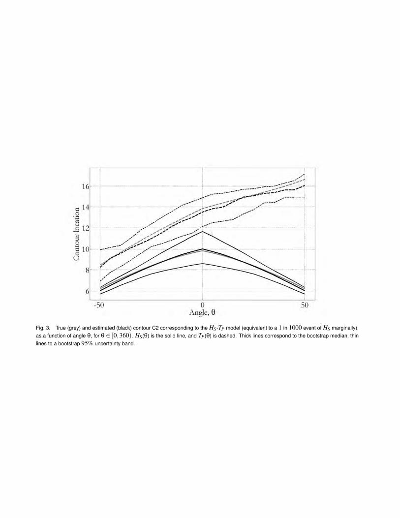
Fig. 3. True (grey) and estimated (black) contour C2 corresponding to the HS-TP model (equivalent to a 1 in 1000 event of HS marginally),as a function of angle θ, for θ ∈ [0,360). HS(θ) is the solid line, and TP(θ) is dashed. Thick lines correspond to the bootstrap median, thinlines to a bootstrap 95% uncertainty band.

Fig. 4. True (grey) and estimated (black) contour C3 corresponding to the HS-TP model (equivalent to a 1 in 1000 event of HS marginally),as a function of angle θ, for θ ∈ [0,360). HS(θ) is the solid line, and TP(θ) is dashed. Thick lines correspond to the bootstrap median, thinlines to a bootstrap 95% uncertainty band.

Fig. 5. True (grey) and estimated (black) contour C4 corresponding to the HS-TP model (equivalent to a 1 in 1000 event of HS marginally),as a function of angle θ, for θ ∈ [0,360). HS(θ) is the solid line, and TP(θ) is dashed. Thick lines correspond to the bootstrap median, thinlines to a bootstrap 95% uncertainty band.
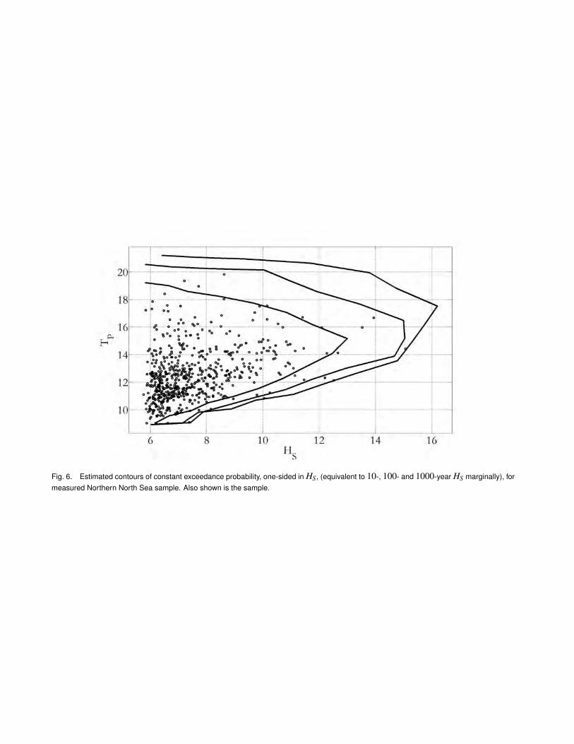
Fig. 6. Estimated contours of constant exceedance probability, one-sided in HS, (equivalent to 10-, 100- and 1000-year HS marginally), formeasured Northern North Sea sample. Also shown is the sample.
Fig. 7. Estimated contours of constant exceedance probability, one-sided in HS, (equivalent to 10-, 100- and 1000-year HS marginally), forhindcast Northern North Sea sample. Also shown is the sample.

Fig. 8. Estimated contours of constant exceedance probability, one-sided in HS, (equivalent to 10-, 100- and 1000-year HS marginally), formeasured Gulf of Mexico sample. Also shown is the sample.
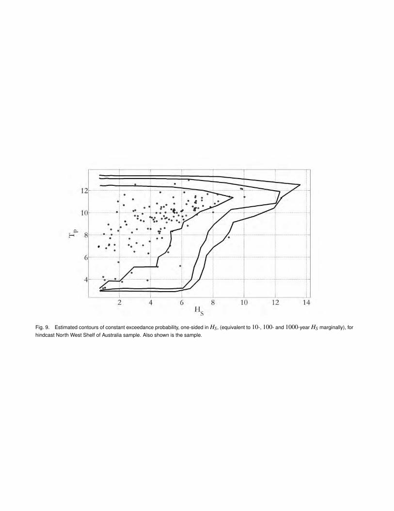
Fig. 9. Estimated contours of constant exceedance probability, one-sided in HS, (equivalent to 10-, 100- and 1000-year HS marginally), forhindcast North West Shelf of Australia sample. Also shown is the sample.
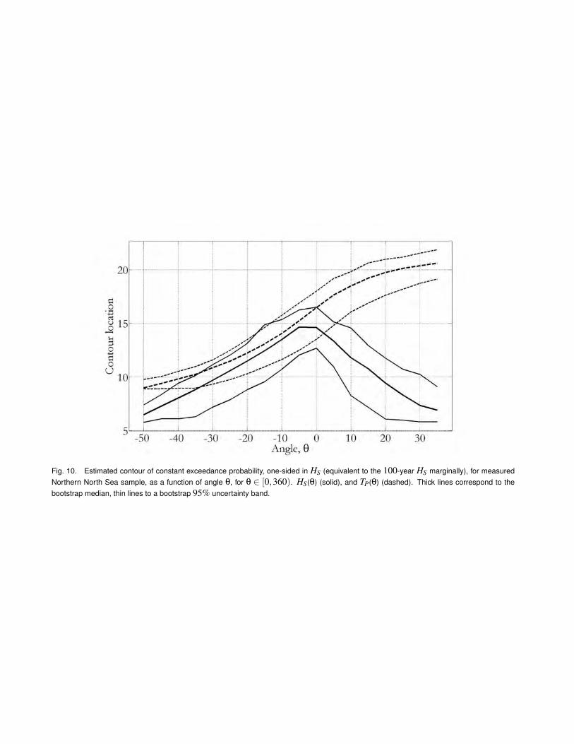
Fig. 10. Estimated contour of constant exceedance probability, one-sided in HS (equivalent to the 100-year HS marginally), for measuredNorthern North Sea sample, as a function of angle θ, for θ ∈ [0,360). HS(θ) (solid), and TP(θ) (dashed). Thick lines correspond to thebootstrap median, thin lines to a bootstrap 95% uncertainty band.
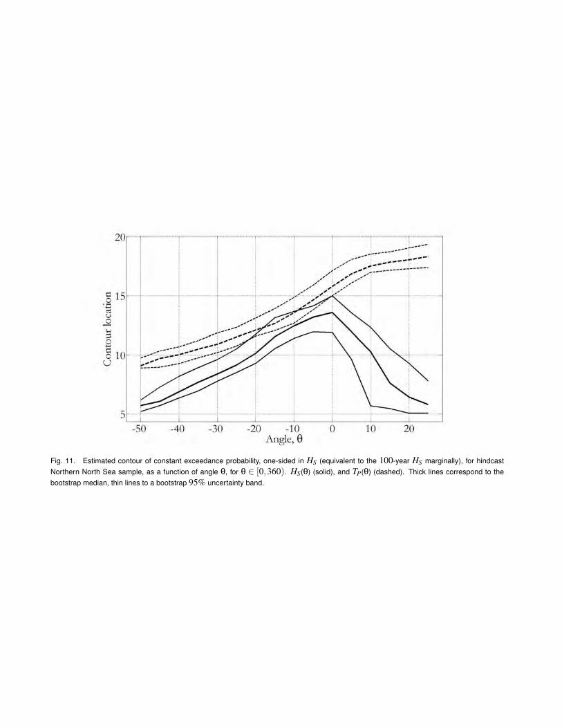
Fig. 11. Estimated contour of constant exceedance probability, one-sided in HS (equivalent to the 100-year HS marginally), for hindcastNorthern North Sea sample, as a function of angle θ, for θ ∈ [0,360). HS(θ) (solid), and TP(θ) (dashed). Thick lines correspond to thebootstrap median, thin lines to a bootstrap 95% uncertainty band.

Fig. 12. Estimated contour of constant exceedance probability, one-sided in HS (equivalent to the 100-year HS marginally), for measuredGulf of Mexico sample, as a function of angle θ, for θ ∈ [0,360). HS(θ) (solid), and TP(θ) (dashed). Thick lines correspond to the bootstrapmedian, thin lines to a bootstrap 95% uncertainty band.

Fig. 13. Estimated contour of constant exceedance probability, one-sided in HS (equivalent to the 100-year HS marginally), for hindcastNorth West Shelf of Australia sample, as a function of angle θ, for θ ∈ [0,360). HS(θ) (solid), and TP(θ) (dashed). Thick lines correspondto the bootstrap median, thin lines to a bootstrap 95% uncertainty band.
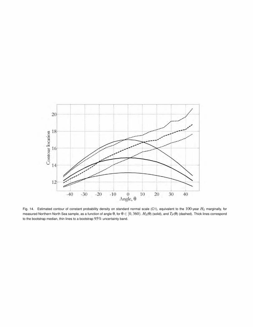
Fig. 14. Estimated contour of constant probability density on standard normal scale (C1), equivalent to the 100-year HS marginally, formeasured Northern North Sea sample, as a function of angle θ, for θ ∈ [0,360). HS(θ) (solid), and TP(θ) (dashed). Thick lines correspondto the bootstrap median, thin lines to a bootstrap 95% uncertainty band.

Fig. 15. Estimated contour of constant probability density on standard normal scale (C1), equivalent to the 100-year HS marginally, forhindcast Northern North Sea sample, as a function of angle θ, for θ ∈ [0,360). HS(θ) (solid), and TP(θ) (dashed). Thick lines correspondto the bootstrap median, thin lines to a bootstrap 95% uncertainty band.

Fig. 16. Estimated contour of constant probability density on standard normal scale (C1), equivalent to the 100-year HS marginally, formeasured Gulf of Mexico sample, as a function of angle θ, for θ ∈ [0,360). HS(θ) (solid), and TP(θ) (dashed). Thick lines correspond tothe bootstrap median, thin lines to a bootstrap 95% uncertainty band.
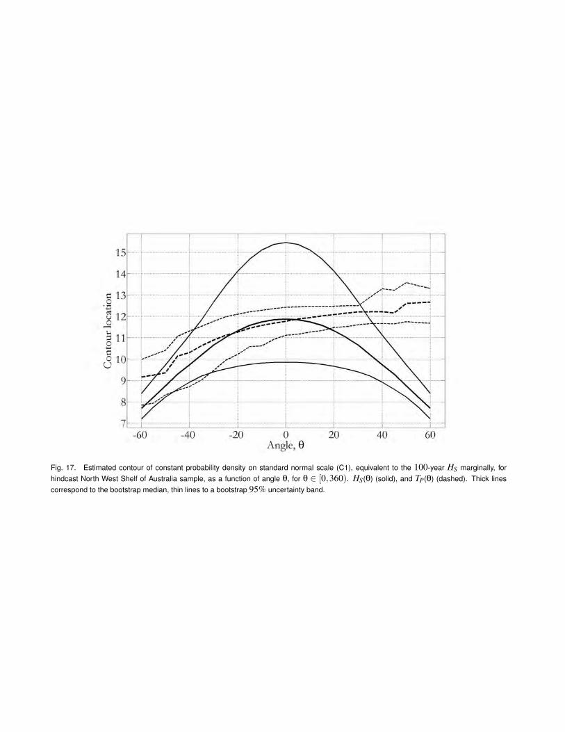
Fig. 17. Estimated contour of constant probability density on standard normal scale (C1), equivalent to the 100-year HS marginally, forhindcast North West Shelf of Australia sample, as a function of angle θ, for θ ∈ [0,360). HS(θ) (solid), and TP(θ) (dashed). Thick linescorrespond to the bootstrap median, thin lines to a bootstrap 95% uncertainty band.