Framework for Residual-Based Error

Estimation in Computational Fluid

Dynamics

Christopher J. Roy

Aerospace and Ocean Engineering Dept.

Virginia Tech

cjroy@vt.edu

V&V Workshop

University of Notre Dame

October 18, 2011

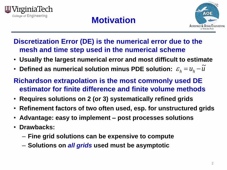
Discretization Error (DE) is the numerical error due to the

mesh and time step used in the numerical scheme

• Usually the largest numerical error and most difficult to estimate

• Defined as numerical solution minus PDE solution:

Richardson extrapolation is the most commonly used DE

estimator for finite difference and finite volume methods

• Requires solutions on 2 (or 3) systematically refined grids

• Refinement factors of two often used, esp. for unstructured grids

• Advantage: easy to implement – post processes solutions

• Drawbacks:

– Fine grid solutions can be expensive to compute

– Solutions on all grids used must be asymptotic

Motivation

2

uuhh~

Example problem: 1D steady Burgers’ equation

• PDE (strong) form:

• Governing equation (PDE or integral eqn.):

• Discrete equation (FDM or FVM):

• Since the PDE operates on a continuous function, and the

discrete solutions exist only at nodes or cell centers, we

will use the following interpolation ( I ) operators

– Prolongation of uh to a continuous space:

– Restriction of to mesh h:

Governing Equation

and Notation

3

0)~( uL

02

2

dx

ud

dx

udu

0)( hh uL

u~ uI h ~

hh uI

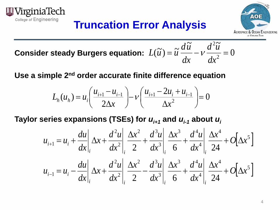
Consider steady Burgers equation:

Use a simple 2nd order accurate finite difference equation

Taylor series expansions (TSEs) for ui+1 and ui-1 about ui

Truncation Error Analysis

0~~

~)~(2

2

dx

ud

dx

uduuL

02

2)(

2

1111

x

uuu

x

uuuuL iiiii

ihh

54

4

43

3

32

2

2

12462

xOx

dx

udx

dx

udx

dx

udx

dx

duuu

iiii

ii

54

4

43

3

32

2

2

12462

xOx

dx

udx

dx

udx

dx

udx

dx

duuu

iiii

ii

4

Plugging in these TSEs and rearranging gives:

Lh(u) L(u) Truncation Error, TEh(u)

This is the Generalized Truncation Error Expression (GTEE)*

This expression holds for any sufficiently smooth function

• Discrete DE:

• Continuous DE:

Generalized Truncation

Error Expression

42

3

32

4

4

2

2

2

1111

612

2

2xO

x

dx

udu

x

dx

ud

dx

ud

dx

duu

x

uuu

x

uuu

i

i

iii

iiiiii

i

5

)~()~()~( wTEwLIwIL h

hh

h

*Roy, C. J. (2009). “Strategies for Driving Mesh Adaptation in CFD (Invited),” AIAA Paper

2009-1302, 47th AIAA Aerospace Sciences Meeting, Orlando, FL, January 5-8, 2009.

2nd Order

w~

uIu h

hh~

uuI hh~

GTEE:

• Plugging in the numerical solution gives:

Continuous Residual

– Similar to the finite element residual

– Requires prolongation of uh to a continuous space for

FDM and FVM

• Plugging in the exact solution to the PDEs gives:

Discrete Residual

Relationship between

Residuals and TE

6

)()()( uTEuLIuIL h

hh

h

)~()~( uTEuIL h

h

h

)()( hhhhh

h uITEuILI

hhuI

We will examine the following residual-based DE

estimators for finite difference and finite volume

methods (most commonly used for CFD)

• DE transport equations

• Defect correction

• Adjoint methods (time permitting)

All three have both continuous and discrete

formulations

Residual-Based DE Estimation

7

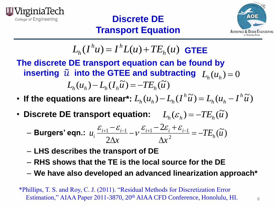
GTEE

The discrete DE transport equation can be found by

inserting into the GTEE and subtracting

• If the equations are linear*:

• Discrete DE transport equation:

– Burgers’ eqn.:

– LHS describes the transport of DE

– RHS shows that the TE is the local source for the DE

– We have also developed an advanced linearization approach*

Discrete DE

Transport Equation

8

)~()~()( uTEuILuL hhhhh

)~()~()( uIuLuILuL h

hh

h

hhh

)~()( uTEL hhh

)~(2

2 2

1111 uTExx

u hiiiii

i

)()()( uTEuLIuIL h

hh

h

0)( hh uL

*Phillips, T. S. and Roy, C. J. (2011). “Residual Methods for Discretization Error

Estimation,” AIAA Paper 2011-3870, 20th AIAA CFD Conference, Honolulu, HI.

Defect correction methods originally developed in the

1970s for ODEs (e.g., Stetter, 1978) two main types:

• Differential correction (continuous defect correction)

– Original problem: solved exactly by (unknown)

– Approximate problem: solved exactly by uh

– Nearby problem: solved exactly by

– Approx. nearby prob.: solved by

– Exact DE in nearby problem is known:

– DE in two problems should be similar:

• Difference correction is similar, but L is replaced by

a discrete operator that is higher order than Lh

(discrete defect correction)

Defect Correction Methods

9

0)( uLh

0)( uL u~

)()( hhuILuL

)()( hh

h

h uILIuL hu

hhh uu

hhhh uu

hL

hhuI

First, form the Lagrangian:

Now, linearize J and L about the function u:

&

Insert these linearizations:

Rearrange combining terms with

The term in brackets will be driven to zero by solving the

adjoint problem

Continuous Adjoint

)~(,)~(),~( uLuJu

...~)()~(

uu

u

JuJuJ

u

...~)()~(

uu

u

LuLuL

u

)~()(,)~()()~(,)~( uu

u

LuLuu

u

JuJuLuJ

uu

=0

)~(,)(,)()~( uuu

L

u

JuLuJuJ

uu

)~( uu

10

Replace

The adjoint problem is solved as:

Thus giving:

Or, accounting for integration errors:

A discrete adjoint could be found similarly which uses the

discrete residual:

Continuous Adjoint (cont’d)

)~(,)(,)()~( h

uu

hhh uuu

L

u

JuLuIJuJ

hh

hhuIu

hhhh uI

uI u

J

u

L

,

)(,)()~( hhhh uILuIJuJ

)(,)~()( nintegratio hhhhh uILuJuJ

)~()~()( nintegratio uILuJuJ h

h

T

hhh

11

The reliability of ALL DE estimators depends on the

numerical solution(s) being in the asymptotic range

• Need to compute the observed order of accuracy

• Given solutions on two systematically-refined meshes by

the factor r, the observed order of accuracy for residual-

based methods is given by (e.g.):

Functionals:

(scalars):

The observed order of accuracy will only match the formal

order when both solutions are asymptotic

Richardson extrap. requires three asymptotic solutions

Reliability of DE Estimates

12

rp h

rh

ln

ln

ˆ

1D Burgers equation for a steady, viscous shock wave

Equation: Exact Sol.:

• Explicit, finite-difference discretization on uniform mesh

• We will examine

– Richardson extrapolation

– Continuous DETE*

– Discrete DETE*

– Defect correction

*simple and advanced

linearizations

Example: Burgers’ Equation

13

02

2

dx

ud

dx

duu

L

xxu

2

Retanh2)(~

33 Nodes 65 Nodes

Results*: Burgers’ Equation

Reynolds Number = 32

14

x (m)

Dis

cre

tiza

tio

nE

rro

r(m

/s)

-1.5 -1 -0.5 0

0

0.05

0.1

Richardson Extrapolation

Continuous DETE (simple)

Discrete DETE (simple)

Continuous DETE

Discrete DETE

Defect Correction

True Error

Reynolds Number = 32, 33 Nodes

x (m)

Dis

cre

tiza

tio

nE

rro

r(m

/s)

-1.5 -1 -0.5 0

0

0.01

0.02

Richardson Extrapolation

Continuous DETE (simple)

Discrete DETE (simple)

Continuous DETE

Discrete DETE

Defect Correction

True Error

Reynolds Number = 32, 65 Nodes

*C. J. Roy, “Survey of Residual-based Methods for Estimating Discretization Error

(Invited),” American Nuclear Society: 2010 Winter Meeting and Nuclear Technology

Expo, November 7-11, 2010, Las Vegas, Nevada

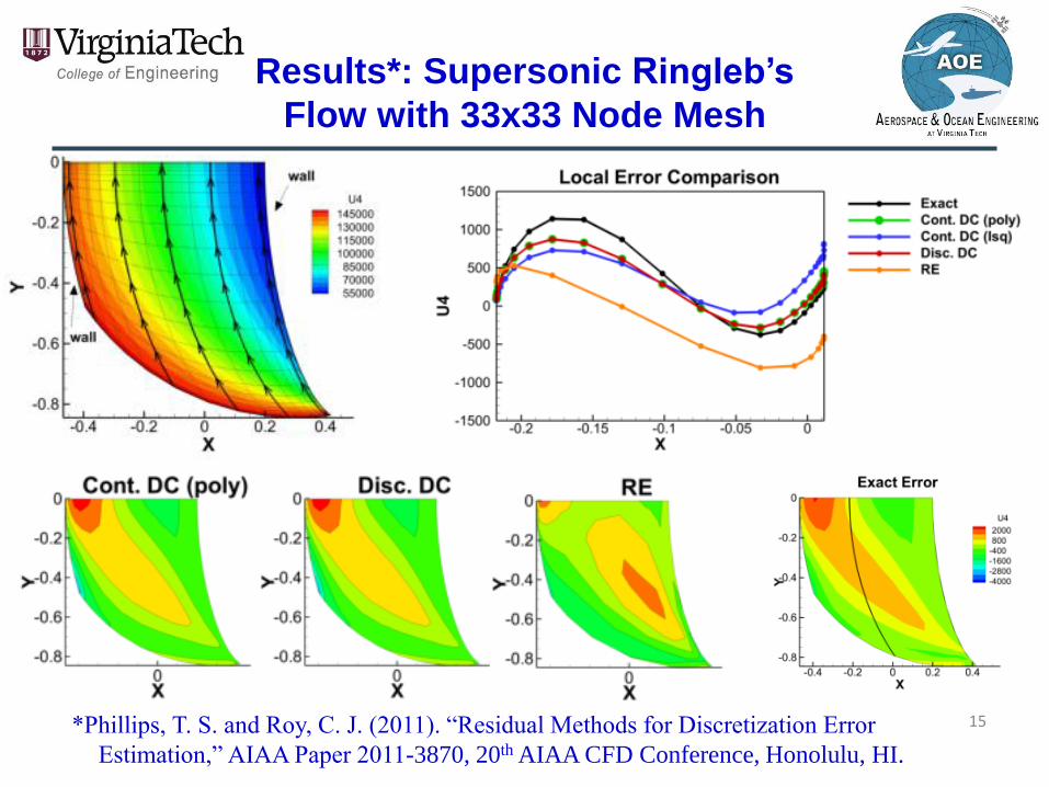
Results*: Supersonic Ringleb’s

Flow with 33x33 Node Mesh

15 *Phillips, T. S. and Roy, C. J. (2011). “Residual Methods for Discretization Error

Estimation,” AIAA Paper 2011-3870, 20th AIAA CFD Conference, Honolulu, HI.

• A framework was presented for developing residual-based

DE estimators in FDM and FVM

• The framework is based on the GTEE which relates the

discrete equations to the PDE/integral equations in a

general manner through the truncation error (TE)

• Assessing the reliability of DE estimators requires at least

two systematically-refined grids to demonstrate that the

solutions are asymptotic

• Simple example problem: Burgers’ equation

– Residual-based methods performed better than Richardson

extrapolation near the asymptotic range

– Not surprising since they require only a single grid and they

also use additional information about the problem

Conclusions

16

I would like to thank my graduate students Tyrone

Phillips, Aniruddha Choudhary, and Joe Derlaga for

their contributions to this residual-based DE

framework

This work was partially supported by Sandia National

Laboratories under a Presidential Early Career Award

for Scientists and Engineers (PECASE).

Acknowledgments

17

Questions???

18