On the Decadal Variability of the Eddy Kinetic Energy in theKuroshio Extension

YANG YANG

School of Atmospheric Sciences, Nanjing University of Information Science and

Technology, Nanjing, China

X. SAN LIANG

School of Marine Sciences, and School of Atmospheric Sciences, Nanjing University of Information

Science and Technology, Nanjing, China

BO QIU AND SHUIMING CHEN

Department of Oceanography, University of Hawai’i at M�anoa, Honolulu, Hawaii

(Manuscript received 29 August 2016, in final form 4 March 2017)

ABSTRACT

Previous studies have found that the decadal variability of eddy kinetic energy (EKE) in the upstream

Kuroshio Extension is negatively correlated with the jet strength, which seems counterintuitive at first glance

because linear stability analysis usually suggests that a stronger jet would favor baroclinic instability and thus

lead to stronger eddy activities. Using a time-varying energetics diagnostic methodology, namely, the lo-

calized multiscale energy and vorticity analysis (MS-EVA), and the MS-EVA-based nonlinear instability

theory, this study investigates the physical mechanism responsible for such variations with the state estimate

from the Estimating the Circulation and Climate of theOcean (ECCO), Phase II. For the first time, it is found

that the decadal modulation of EKE is mainly controlled by the barotropic instability of the background flow.

During the high-EKE state, violent meanderings efficiently induce strong barotropic energy transfer from

mean kinetic energy (MKE) to EKE despite the rather weak jet strength. The reverse is true in the low-EKE

state. Although the enhanced meander in the high-EKE state also transfers a significant portion of energy

frommean available potential energy (MAPE) to eddy available potential energy (EAPE) through baroclinic

instability, the EAPE is not efficiently converted to EKE as the two processes are not well correlated at low

frequencies revealed in the time-varying energetics. The decadal modulation of barotropic instability is found

to be in pace with the North Pacific Gyre Oscillation but with a time lag of approximately 2 years.

1. Introduction

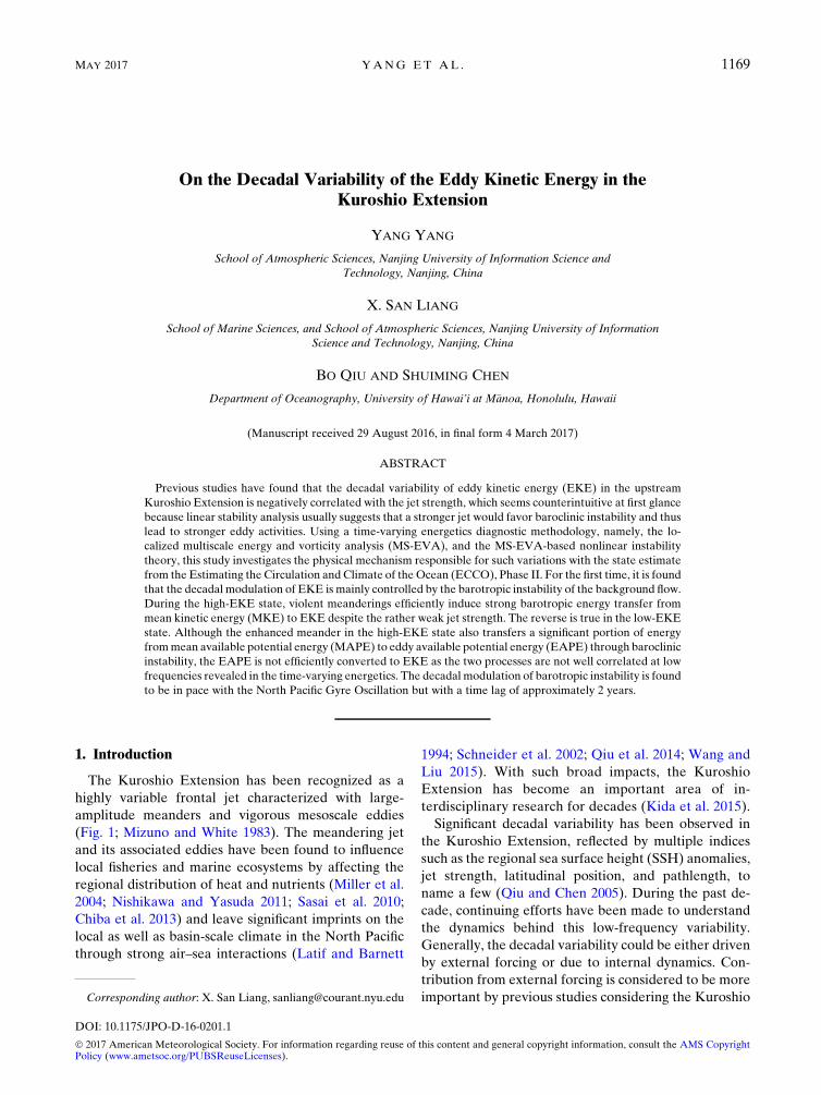
The Kuroshio Extension has been recognized as a

highly variable frontal jet characterized with large-

amplitude meanders and vigorous mesoscale eddies

(Fig. 1; Mizuno and White 1983). The meandering jet

and its associated eddies have been found to influence

local fisheries and marine ecosystems by affecting the

regional distribution of heat and nutrients (Miller et al.

2004; Nishikawa and Yasuda 2011; Sasai et al. 2010;

Chiba et al. 2013) and leave significant imprints on the

local as well as basin-scale climate in the North Pacific

through strong air–sea interactions (Latif and Barnett

1994; Schneider et al. 2002; Qiu et al. 2014; Wang and

Liu 2015). With such broad impacts, the Kuroshio

Extension has become an important area of in-

terdisciplinary research for decades (Kida et al. 2015).

Significant decadal variability has been observed in

the Kuroshio Extension, reflected by multiple indices

such as the regional sea surface height (SSH) anomalies,

jet strength, latitudinal position, and pathlength, to

name a few (Qiu and Chen 2005). During the past de-

cade, continuing efforts have been made to understand

the dynamics behind this low-frequency variability.

Generally, the decadal variability could be either driven

by external forcing or due to internal dynamics. Con-

tribution from external forcing is considered to be more

important by previous studies considering the KuroshioCorresponding author: X. San Liang, sanliang@courant.nyu.edu

MAY 2017 YANG ET AL . 1169

DOI: 10.1175/JPO-D-16-0201.1

� 2017 American Meteorological Society. For information regarding reuse of this content and general copyright information, consult the AMS CopyrightPolicy (www.ametsoc.org/PUBSReuseLicenses).

Extension’s linear response to the incoming westward

propagation of large-scale baroclinic Rossby waves,

which was forced by anomalous wind stress curl in the

central North Pacific (Miller et al. 1998; Deser et al.

1999; Seager et al. 2001; Qiu 2003; Kwon and Deser

2007; Ceballos et al. 2009; Sasaki and Schneider 2011).

On the other hand, the intrinsic mechanism claimed that

the decadal variability is an internal mode of the highly

nonlinear western boundary current (WBC) system,

which is confirmed in a variety of numerical models

ranging from idealized quasigeostrophic models to re-

alistic ocean general circulation models (OGCMs;

McCalpin and Haidvogel 1996; Simonnet and Dijkstra

2002; Hogg et al. 2005; Nonaka et al. 2006; Berloff et al.

2007; Primeau and Newman 2008; Pierini et al. 2009).

Internal processes, such as instabilities and eddy–mean

flow interactions, whether they are self-sustained or

modulated by external forcing, are indispensable in-

gredients to achieve a full understanding of the dy-

namics underlying the decadal variability in this region.

Baroclinic instability has been recognized as the primary

source of eddy kinetic energy (EKE) in the global ocean

(Gill et al. 1974; Ferrari andWunsch 2009; von Storch et al.

2012). Mesoscale eddies derive much of their energy from

the available potential energy (APE) of the large-scale

mean flow (Pedlosky 1987).Hence, it is generally expected

that the eddy activity in WBCs should be stronger when

the mean flow is more baroclinic. Recent studies based on

satellite observations and numerical simulations have re-

ported that the low-frequency (interannual to decadal)

changes of EKE in several ocean sectors are indeed con-

trolled by baroclinic instability of the background currents,

for example, the North Atlantic Ocean (Penduff et al.

2004), the southeast Indian Ocean (Jia et al. 2011), the

Azores Current (Volkov and Fu 2011), the western North

Pacific Subtropical Gyre (Qiu and Chen 2013), and the

northeastern South China Sea (Sun et al. 2016). Unlike

those regions where the low-frequency EKE variability is

largely in phase with the baroclinicity of the background

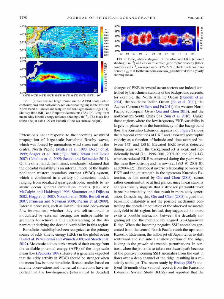
flow, the Kuroshio Extension appears not. Figure 2 shows

the temporal variations of EKE and eastward geostrophic

velocity as a function of latitude and time averaged be-

tween 1428 and 1508E. Elevated EKE level is detected

during years when the background jet is weak and me-

ridionally broad (i.e., 1996–2001, 2005–09, and 2013–14),

whereas reduced EKE is observed during the years when

themean flow is strong and narrow (i.e., 1993–95, 2002–05,

and 2009–12). This robust inverse relationship between the

EKE and the jet strength in the upstream Kuroshio Ex-

tension, as first noted by Qiu and Chen (2005), seems

rather counterintuitive at first glance, since linear stability

analysis usually suggests that a stronger jet would favor

baroclinic instability and thus result in more eddy gener-

ation. Considering this, Qiu and Chen (2005) argued that

baroclinic instability is not the possible mechanism con-

trolling the decadal modulation of the observedmesoscale

eddy field in this region. Instead, they suggested that there

exists a possible interaction between the decadally mi-

grating jet and the meridionally aligned Izu–Ogasawara

Ridge. When the incoming negative SSH anomalies gen-

erated from the central North Pacific reach the upstream

Kuroshio Extension, the inflow jet off Japan tends to shift

southward and run into a shallow portion of the ridge,

leading to the growth of unstable perturbations. In con-

trast, when the jet tends to take a northward path because

of the positive incoming SSH anomalies from the east, it

flows over a deep channel of the ridge, resulting in a rel-

atively stable jet. The recent study by Bishop (2013) ana-

lyzed 16-month observational records from the Kuroshio

Extension System Study (KESS) and reported that the

FIG. 1. (a) Sea surface height based on the AVISO data (white

contours; cm) and bathymetry (colored shading; m) in the western

North Pacific. Labeled in the figure are Izu–OgasawaraRidge (IO),

Shatsky Rise (SR), and Emperor Seamounts (ES). (b) Long-term

mean eddy kinetic energy (colored shading; Jm23). The black line

shows the jet axis (100-cm isobath of the sea surface height).

FIG. 2. Time_latitude diagram of the observed EKE (colored

shading; Jm23) and eastward surface geostrophic velocity (black

contours; cm s21) averaged over 1428–1508E. Thick black contours

denote ugeo5 0. Both time series are low_pass filtered with a yearly

running mean.

1170 JOURNAL OF PHYS ICAL OCEANOGRAPHY VOLUME 47

vertical coupling between the deep eddies and the upper

jet is consistent with a baroclinic instability scenario after

the regime shifts from a stable state to an unstable state.

Up to now, we are unware of any other studies focusing on

themechanism that gives rise to this peculiar decadal EKE

variability in the upstreamKuroshio Extension. Questions

like, but not limited to, the following are still to be ad-

dressed. Since it is found that the eddy activities are neg-

atively correlated to the jet strength, which by the linear

instability theory is correlated to the strength of baroclinic

instability, one naturally wants to know whether indeed

baroclinic instability is reduced when eddy activities are

strong. If so, then, what is the mechanism governing the

eddy growth, and what processes are involved in the low-

frequency eddy modulation?

In this study, we address these issues by analyzing the

time-varying eddy energetics. A multiscale energetics

study in the time-varying sense is a notorious challenge

in geophysical fluid dynamics. A recent comprehensive

investigation is referred to Liang (2016); in section 2,

we will give a brief introduction of the part relevant to

this study. Another difficulty for the analysis is the

short temporal coverage of in situ observation (e.g.,

KESS), while the information obtained from satellite

altimetry is merely surface limited. We will hence use

the available reanalysis data instead. Based on an

eddy-resolving global hindcast model, the long-

term climatology of the multiscale energetics in the

Kuroshio Extension was recently addressed by Yang

and Liang (2016). They found that the baroclinic en-

ergy pathway, transferringmeanAPE (MAPE) to eddy

APE (EAPE) and finally converting to EKE, together

with the barotropic energy pathway, transferring mean

kinetic energy (MKE) to EKE, are equally important

for the growth of the EKE in the upstream region of

Kuroshio Extension. However, the energetics they

examined is in a statistical mean sense; no time varia-

tion was considered. Although, as suggested by pre-

vious studies (Qiu and Chen 2005) that the baroclinic

pathway can be potentially ruled out for the decadal

changes in mesoscale eddy variability in this region,

this first-guess argument has not considered the fact

that the Kuroshio Extension, especially the upstream

portion of it, is significantly nonzonal. Several studies

have reported even weak nonzonal currents can lead to

strong instabilities (e.g., Spall 2000; Smith 2007). The

nonzonal component of the jet, as manifested by its

meanderings, has been recognized to induce significant

energy transfer from the mean flow to the eddies

through efficient barotropic and baroclinic instability

(Abernathey and Cessi 2014; Bischoff and Thompson

2014; Chapman et al. 2015; Chen et al. 2015; Elipot and

Beal 2015). Thus, quantifying baroclinic instability and

barotropic instability from the data is the key to un-

covering the underlying dynamics of the decadal EKE

modulation in the Kuroshio Extension system. Re-

cently, Liang and Robinson (2005, 2007) developed a

localized, finite-amplitude instability analysis, which is

based on the localized multiscale energy and vorticity

analysis (MS-EVA); it proves to be very efficient in

diagnosing the nonlinear eddy–mean flow interactions

and multiscale instabilities in real oceanic and atmo-

spheric processes (Liang and Robinson 2009; Yang and

Liang 2016). In the formalism, contributions from

baroclinic and barotropic instabilities to the eddy en-

ergy generation as well as other sources, sinks, and

redistributions of eddy energy can be explicitly com-

puted. In this study, we will apply MS-EVA and the

MS-EVA-based finite-amplitude hydrodynamic in-

stability theory to investigate the instabilities and en-

ergetics associated with the decadal EKE modulation

in the upstream Kuroshio Extension. The rest of the

paper is organized as follows: We briefly introduce the

MS-EVA in section 2 and the data description and

validation in section 3. The major results are presented

in section 4. They are then discussed and summarized in

section 5.

2. Methodology

Ever since the Lorenz (1955) energy cycle was in-

troduced in the atmosphere science, energetics analysis

has become a powerful tool to diagnose the intrinsic

and external energy sources and sinks and flow in-

stabilities. Thus, it is natural to evaluate the decadal

EKE variations in the Kuroshio Extension from the

perspective of time-dependent energetics analysis,

which, to our knowledge, has not been documented

before [what Yang and Liang (2016) investigated is

long-term mean energetics in this region]. In this sec-

tion, we present a brief introduction of the localized

MS-EVA and the MS-EVA-based theory of finite-

amplitude baroclinic and barotropic instability; for

details, see the references cited thereof.

Time-varying energetics analysis is a continuing

challenge in geophysical fluid dynamics. Recently,

Liang (2016) gave this a comprehensive review and

elucidated the theoretical challenges and clarified

some misconceptions currently in existence. In this

study, we use the multiscale window transform

(MWT) of Liang and Anderson (2007) to decompose

the original fields into two orthogonal windows,

namely, a low-frequency mean flow window and a

high-frequency eddy window. To emphasize the con-

tribution from the mesoscale eddy signals, the cutoff

period of the window decomposition is set to 260 days,

MAY 2017 YANG ET AL . 1171

which is consistent with the previous eddy character-

istics studies of this region (Itoh and Yasuda 2010). We

have tested the periods varying from 6 months to 2

years, and the results are all quantitatively similar. For

easy reference, the mean flow window and the eddy

window are denoted by - 5 0, 1, respectively. Within

the MWT framework, the kinetic energy (KE) and

APE on window - are

K- 51

2r0u;-H � u;-

H , and (1)

A- 5g2

2r0N2

(r;-)2 , (2)

respectively, where g is the acceleration due to gravity,

uH 5 (u, y) is the horizontal velocity vector, r0 is the

reference density, r is the density perturbation from

the background profile r(z), N5ffiffiffiffiffiffiffiffiffiffiffiffiffiffiffiffiffiffiffiffiffiffiffiffiffiffiffi2g(›r/›z)/r0

pis

the buoyancy frequency, and c(�);-denotes MWT on

window -. A detailed derivation of the K- and A-

equations are referred to Liang (2016); here, the results

are summarized below:

›K-

›t1 = �

�1

2r0u;- d(uu

H);-

�|fflfflfflfflfflfflfflfflfflfflfflfflfflfflfflfflfflffl{zfflfflfflfflfflfflfflfflfflfflfflfflfflfflfflfflfflffl}

=�Q-K

52= � (u;-p;-)|fflfflfflfflfflfflfflfflfflffl{zfflfflfflfflfflfflfflfflfflffl}=�Q-

P

2

�1

2r0(u;-)2= � u-

u 11

2r0(y;-)2= � u-

y

�|fflfflfflfflfflfflfflfflfflfflfflfflfflfflfflfflfflfflfflfflfflfflfflfflfflfflfflfflfflfflfflfflfflfflfflfflffl{zfflfflfflfflfflfflfflfflfflfflfflfflfflfflfflfflfflfflfflfflfflfflfflfflfflfflfflfflfflfflfflfflfflfflfflfflffl}

G-K

1 (2gr;-w;-)|fflfflfflfflfflfflfflfflfflffl{zfflfflfflfflfflfflfflfflfflffl}b-

1F-K ,

(3)

and›A-

›t1 = �

�g2

2r0N2

r;- d(ru);-�

|fflfflfflfflfflfflfflfflfflfflfflfflfflfflfflfflfflfflfflffl{zfflfflfflfflfflfflfflfflfflfflfflfflfflfflfflfflfflfflfflffl}=�Q-

A

5 2A-= � u-r|fflfflfflfflfflfflfflffl{zfflfflfflfflfflfflfflffl}

G-A

1 gr;-w;-|fflfflfflfflfflffl{zfflfflfflfflfflffl}2b-

1F-A , (4)

where u 5 (u, y, w) is the three-dimensional velocity

vector, and p is the dynamic pressure. The terms u-u , u

-y ,

and u-r are referred to as the T-coupled velocity, which

satisfies u-T 5

d(uT);-/T;- for T 5 u, y, or r.

In (3) and (4), the G- terms represent the local process

of cross-scale energy transfer to window -. Recently,

Liang (2016) proved that they actually can be written

in a Lie bracket form, just like the Poisson bracket in

Hamiltonian mechanics. The = �Q- terms denote the

nonlocal process of energy flux divergence through ad-

vection or pressure work; positive (negative) values rep-

resent the energy transporting out of (into) the local

domain. The b- term is the rate of buoyancy conversion

connecting APE and KE. The external forcing and in-

ternal dissipation processes [denoted as F in (3) and (4)]

are not explicitly calculated but considered as a residual

in this study. Notice that the above terms in (3) and (4)

are all four-dimensional field variables and so have all the

localized information retained, which is essential for

the diagnosis of the decadally varying eddy energetics in

the Kuroshio Extension. Particularly, the transfer term

G- has an interesting property, namely,

�-�n

G-n 5 0, (5)

where �n is a summation over all the sampling time

steps n [the subscript n is omitted through (1)–(4) for

simplicity], and �- is a summation over all scale win-

dows - [see Liang (2016) for details]. Notice that the

transfer terms in the traditional formalism will sum to a

divergence form that has zero global-mean values but

nonzero local values. This makes the local in-

terpretation of the cross-scale energy transfer process a

difficult one since physically an energy transfer process

should merely redistribute energy among scales

(Rhines 1977; Cai et al. 2007; Liang and Robinson

2005). To distinguish, this process in the MS-EVA

formalism is termed ‘‘canonical transfer.’’ The canonical

transfer is important in that they are closely related to the

classical geophysical fluid dynamics (GFD) stability the-

ory. Details can be found in Liang and Robinson (2007)

and Liang (2016). In this study, we use the superscript

-0 / -1 to signify such window-to-window interactions

and hence instabilities. Physically, a positive baroclinic

(barotropic) transfer rate from the mean–flow window

(- 5 0) to the eddy window (- 5 1) is indicative of

baroclinic (barotropic) instability in the ocean. Figure 3

illustrates the energy diagram for a two-window

decomposition.

3. Data description and validation

We use the model outputs from Estimating the Cir-

culation and Climate of the Ocean (ECCO), Phase II

(ECCO2) as the input of MS-EVA application. ECCO2

1172 JOURNAL OF PHYS ICAL OCEANOGRAPHY VOLUME 47

is based on the Massachusetts Institute of Technology

General Circulation Model (MITgcm; Marshall et al.

1997), which is a 3D, z-level, hydrostatic, Boussinesq

ocean model, using cube sphere grid projection (cube92

version) with a mean horizontal resolution of 18 km.

Vertically, the model has 50 levels, with resolution

varying from 10m near the sea surface to 456m near the

bottom at a maximum depth of 6150m. The high-

resolution global ocean state estimate is obtained by a

least squares fit of the MITgcm to the available satellite

and in situ data. Using a Green’s function approach

(Menemenlis et al. 2005), the least squares fit is em-

ployed for a number of control parameters (see the ap-

pendix for more information). With these optimized

control parameters, themodel is run forward freely, as in

any ordinary model simulation. Since no data are taken

in to interrupt the forward run, the state estimate is

considered to be dynamically and kinematically consis-

tent (Wunsch et al. 2009). Its high-resolution and

decadal-long (1992–present) global output has been

extensively used to examine the eddy dynamics and

ocean energetics (Fu 2009; Zemskova et al. 2015; Chen

et al. 2016). In this study, the 3-day-averaged dataset

over 1993–2015 is used.

Simulating the phase evolution of frontal processes

and the associatedmesoscale eddy fields in the Kuroshio

Extension region is a challenge because of the highly

nonlinear and stochastic nature of the WBC system. In

contrast, large-scale oceanic linear features, such as

baroclinic Rossby waves, can be easily reproduced in

numerical hindcast simulations (Qiu 2003; Taguchi et al.

2007). For instance, Taguchi et al. (2010) reported that

salient features of decadal modulation of observed SSH

in the Kuroshio Extension region are well captured in an

eddy-resolving multidecadal ocean model hindcast

simulation, while the modeled EKE in the upstream

Kuroshio Extension region failed to reproduce the ob-

served decadal phase evolution. We have tried some

datasets and identified that the ECCO2 dataset is the

one that has the decadal EKE variability appropriately

simulated in this region (see the appendix). In the fol-

lowing, the SSH data from altimeter satellite products

distributed by the Archiving, Validation, and In-

terpretation of Satellite Oceanographic (AVISO; Ducet

et al. 2000) are used to test the degrees of fidelity of the

ECCO2 state estimate in the Kuroshio Extension.

Generally, the model has well reproduced the long-term

mean surface circulation in the Kuroshio Extension

(vectors in Figs. 4a,b). By conducting an empirical or-

thogonal function (EOF) analysis, we compare the

dominant spatiotemporal mode of EKE obtained from

the ECCO2 state estimate with that from the altimeters.

During the period of 1993–2015, the first EOF mode

accounts for 9.2% and 8.2% (reaches 34.4% and 31.4%

after applying a 1-yr low-pass filter to the original EKE

field) of the total EKE variance for the observation and

the model, respectively. The EOF spatial pattern of the

first mode from the model is similar to that from the

altimetry (colored shades in Figs. 4a,b), both of which

are characterized by a hot spot of variance in the first

quasi-stationary meander region between 328 and 368Nand 1418 and 147.58E. The corresponding principle

component (PC) from the model also captures the ob-

served one favorably well, both of which show higher-

than-normal variations in 1996–2001 and 2005–08 and

lower-than-normal variations in 1993–95 and 2002–04.

The linear correlation coefficient r between the two time

series is 0.41 for the period during 1993–2008. The cor-

responding r between the two low-pass filtered series

(with periods longer than 1 yr; not shown) reaches as

high as 0.72 (statistically significant over the 95% con-

fidence level). Notice that the model results are not well

correlated with the observed one in some individual

years such as 2009, 2011, and 2015. This discrepancymay

result from multiple causes related to the model con-

figurations, which is beyond the scope of the present

study. To conclude this section, in Fig. 4 we plot the

EKE time series averaged over the box of 328–368N and

1428–1528E (see the gray box in Fig. 4b), where the

largest EKE variability occurs. This EKE time series is

found to be dominated by its first EOFmode. The series

FIG. 3. Energy pathway diagram for a two-window de-

composition. Red arrows indicate the energy transfer between the

mean–flow (indicated as superscript 0) and eddy window (indicated

as superscript 1), while navy arrows illustrate the buoyancy con-

version connecting the KE and APE reservoirs. Blue dashed ar-

rows indicate nonlocal processes transporting into or out of the

local ocean domain. The forcing and dissipation processes are de-

noted as F terms (dashed green arrows).

MAY 2017 YANG ET AL . 1173

almost coincides with the first PC series; the linear cor-

relation coefficient between them is as high as 0.92. In

other words, although the EKE variance explained by

the first EOF mode is not so high, this mode effectively

captures the regional coherent EKE variability. Partic-

ularly, the ECCO model successfully reproduced the

two complete decadal cycles of the observed EKE.

Thus, we can safely say that the model outputs are ap-

propriate for the purpose of this study.

4. Results

To examine the spatial difference between the two

dynamical states, composite maps are constructed.

High-EKE and low-EKE states are defined based on the

PC-1 of the simulated EKE (Fig. 4c). The high (low)

phase occurs when the PC-1 series has a value greater

(less) than 1 (21) standard deviation. According to the

definition above, 358 and 317 samples are selected for

the high and low composites, respectively. The com-

posite horizontal maps show that the high-EKE state is

characterized by a spatially coherent strong EKE in the

upstream Kuroshio Extension, while the EKE level re-

duces remarkably during the low-EKE state (color

shades in Figs. 5a,b). To clarify the cause underlying the

contrast between these bimodal states, it is helpful to

examine the associated background circulation differ-

ences. The composite maps of the surface velocity field

(vectors in Figs. 5a,b) capture the contrast in spatial

patterns of the Kuroshio Extension jet and its associated

southern recirculation gyre (SRG) between the two

dynamic states. In the high-EKE state, the eastward-

flowing jet appears broad and convoluted. During the

low-EKE state, the eastward jet takes a straight path and

FIG. 4. First EOF mode of surface EKE from (a) the satellite observation and (b) ECCO2 state estimate. The

spatial patterns (colored shading; Jm23) are obtained by a regression of the EKE onto the normalized PCs of the

EOF modes. The long-term mean of the surface geostrophic circulation (vectors; cm s21) is superposed in each

map. The gray box represents the regionwithmaximumEKEvariance. (c) Normalized principal component (PC-1)

of the observation (red) and ECCO2 state estimate (blue). The horizontal black lines indicate the periods when the

KuroshioExtension system is in the high-EKE state. (d) Normalized EKE time series averaged over the gray box of

Fig. 4b (red), and the series of the first PC of the EKE (blue) from the ECCO2 state estimate.

1174 JOURNAL OF PHYS ICAL OCEANOGRAPHY VOLUME 47

is accompanied by a well-defined SRG south of the jet

axis. The above description of the relationship between

the background circulation state and the regional EKE

in the ECCO2 state estimate is consistent with previous

findings using altimetry observations (Qiu and Chen

2005, 2010), indicating again that the ECCO2 is reliable

for the investigation of the decadal variability of the

EKE in this region. The difference of the circulation

between the two phases exhibits a train of anomalous

cyclonic and anticyclonic circulations over the time-

mean crest and trough (Fig. 5c), indicating that during

the years when eddy activities are strong (weak), the

Kuroshio Extension jet and its associated recirculation

gyres are weak (strong), whereas the meanders are

strong (weak). These results suggest that the decadal

variability of EKE in this region is related to the stability

of the jet’s meanderings. In fact, the importance of sta-

tionary meanders in setting EKE distributions in the

ocean has been reported in several recent studies. For

instance, Abernathey and Cessi (2014) found that the

standing meanders in the Southern Ocean are able to

concentrate the eddy activity and meridional heat flux.

Chapman et al. (2015) proposed that the oceanic storm

tracks could be initiated in standing meanders where

strong localized energy transfer from the mean field to

the eddy field is found. Apart from bringing in elevated

baroclinic instability, stationary meanders are also

responsible for the sudden and strong positive transfer

of KE from the mean flow to the eddies through baro-

tropic instability (Elipot and Beal 2015).

To better reveal the cause of the decadal variation of

the EKE in the upstream Kuroshio Extension, we em-

ploy the MS-EVA for the diagnostics. Generally, the

EKE variability in an ocean domain can be influenced

by direct local wind forcing, nonlinear energy transfers

through barotropic and baroclinic instabilities, in-

teractions between flow and topography, nonlocal pro-

cesses radiated from (or to) the remote region, and

dissipation processes (Gill et al. 1974; Pedlosky 1987;

Garnier and Schopp 1999; Stammer and Wunsch 1999;

Zhai et al. 2008; Yang et al. 2013; Kang et al. 2016). Early

stochastic modeling studies provided evidences of direct

wind-forced eddies in regions of weak currents

(Frankignoul and Müller 1979; Müller and Frankignoul

1981), whereas local wind stress forcing is found not well

correlated with the eddy activity in the vicinity of strong

currents (White andHeywood 1995). In fact, a variety of

observational studies have focused on the covariance

between the Kuroshio Extension indices and atmo-

spheric variables, all suggesting that the ocean-to-

atmosphere forcing dominate the atmosphere-to-ocean

forcing in this region, especially on the decadal time

scale (Nonaka and Xie 2003; Qiu et al. 2014; Seo et al.

2014; O’Reilly and Czaja 2015; Wang and Liu 2015).

FIG. 5. Composite maps of the EKE (colored shading; Jm23) and surface geostrophic circulation (vectors; cm s21)

for (a) the high-EKE state and (b) the low-EKE state and (c) their difference in the ECCO2 state estimate. Hatched

are regions where the corresponding differences are significant at the 95% confidence level.

MAY 2017 YANG ET AL . 1175

Considering this, we will only focus on the time-

dependent barotropic and baroclinic instability pro-

cesses and nonlocal energy advections and their

relations with the decadal EKE variability; processes

related to external forcings such as direct local wind

forcing and flow–topography interactions and dissipa-

tion processes are not addressed in the present study.

a. Baroclinic and barotropic instabilities

Baroclinic and barotropic instabilities have been

considered as the major energy sources for mesoscale

eddies in the Kuroshio Extension (Hall 1991; Waterman

et al. 2011; Yang and Liang 2016). In this subsection, we

focus on the two instabilities, which are measured by the

canonical baroclinic and barotropic transfer (see Liang

2016), respectively. The baroclinic transfer G0/1A , when

positive, is a measure of the energy transfer fromMAPE

to EAPE. Similarly, the barotropic transfer G0/1K , when

positive, is a measure of energy transfer from MKE to

EKE. These two metrics are distinct from classical ones

due to two reasons: first, they only involve processes

among different scale windows and hence are essentially

connected to instabilities in a generalized sense

(Pedlosky 1987; Liang and Robinson 2007); second, they

are time-dependent, four-dimensional field variables,

thus providing the possibility to investigate the temporal

variability of eddy–mean flow interactions and in-

stabilities embedded in the complex dynamics of the

decadally modulating Kuroshio Extension. For conve-

nience, we will refer to the baroclinic and barotropic

transfer as BC and BT, respectively.

In Figs. 6a and 6b, we show the horizontal maps of

the depth-averaged (upper 1000m) BC composites. The

most noticeable feature is that BC is confined along the

FIG. 6. Depth-averaged (upper 1000m) BC maps (colored shading; 1024Wm23) in the (a) high-EKE state and (b) low-EKE state and

(c) zonal-mean structures from the ECCO2 state estimate. SSH composites (contours; cm) in each phase are superposed in (a) and (b).

(d)–(f) As in (a)–(c), but for BT. (g)–(i) As in (a)–(c), but for b1.

1176 JOURNAL OF PHYS ICAL OCEANOGRAPHY VOLUME 47

narrow eastward jet in the low-EKE state, whereas it is

spread out meridionally in the high-EKE state, which is

in good agreement with the violent meanders in this

state. Significant positive BC is found in the deep me-

ander region, suggesting the active role played by

standing meanders to elevate the regional baroclinic

energy transfer. The latitudinal structure of the zonally

averaged BC across the upstreamKuroshio Extension is

shown in Fig. 6c. On average, BC peaks positively along

the mean path, indicating that the eddies extract APE

from the mean flow. During the low-EKE state, BC

peaks at 0.173 1024Wm23 at;368N. In contrast to the

low-EKE state, BC reaches 0.24 3 1024Wm23 at

;348N during the high-EKE state. The southward mi-

gration of the maximum BC from the low-EKE state to

the high-EKE state is in agreement with the southward

shift of the jet. Overall, the above results are consistent

with previous study by Bishop (2013), who also found

the unstable meanders during the high-EKE state

transfer significant APE from the background flow to

the eddies. During the high-EKE state, the eddies are

also found transferringmoreAPE back to themean flow

at several spots, such as 33.88N, 1468E and 368N, 147.58E.In contrast, similar negative BC spots are not clearly

distributed during the low-EKE state. Those negative

BC centers may be related to recurring passages of cold-

core rings during the high-EKE state, as suggested by

Bishop (2013).

Figures 6d and 6e show the barotropic transfer com-

posite maps in the high-EKE state and low-EKE state,

respectively. We see that the horizontal pattern of BT

bears some resemblance with that of BC, which also

peaks positively in the deep meander region during the

high-EKE state, whereas it is confined within the strong

but narrow jet with much reduced amplitude in the low-

EKE years. The latitudinal distribution of the zon-

ally averaged BT clearly shows that the BT peaks at

0.353 1024Wm23 during thehigh-EKEstate, nearly 4 times

larger than that in the low-EKE state (0.093 1024Wm23).

Besides, by comparing Figs. 6c and 6f, we can see that

the violent meanders in the high-EKE state induce en-

ergy transfer from the mean flow to the eddies mainly

through barotropic instability.

The distribution of buoyancy conversion term b1 is

plotted in Figs. 6g and 6h. As indicated in (3) and (4),

this term acts as a proxy connecting theEKE andEAPE.

Notice that it is important to distinguish the aforemen-

tioned BC and b1. As BC measures the cross-scale en-

ergy transfer between the MAPE reservoir and EAPE

reservoir, b1 represents the energy conversion between

the EAPE reservoir and EKE reservoir. The b1 term is

an inseparable part of baroclinic production of EKE

through MAPE / EAPE / EKE pathway. Although

the baroclinic pathway has been recognized as the main

mechanism to generate EKE in the global ocean (von

Storch et al. 2012), it might not be necessarily re-

sponsible for the EKE variation at low frequencies be-

cause the two different stages may not be correlated on

the decadal time scale. Indeed, the composite EAPE

seems to be not efficiently converted to EKE during the

high-EKE state (Fig. 6i). Significant negative centers are

found around the southern tip of the meander trough as

well as the downstream region east of 1508E. A closer

look at the baroclinic pathway (MAPE / EAPE /EKE) and the barotropic energy pathway (MKE /EKE) reveals that there is an interesting seesaw relation

between them (Figs. 6f,i). During the low-EKE state,

the baroclinic pathway is the major energy source of the

EKE reservoir for the entire upstream Kuroshio Ex-

tension, whereas in the high-EKE state, the barotropic

energy pathway prevails and the baroclinic pathway is

suppressed. A similar seesaw relation is also found in a

recent modeling study (Chen et al. 2016), which needs to

be verified in observation.

Figure 7 provides the vertical structure of the ener-

getics during the two different states along the zonal

band of the largest EKE variance. During the low-EKE

state, bothBC and b1 peak at a narrow band surrounding

the jet axis where the largest isopycnal slope is observed

(Figs. 7b,d). In contrast, the largest BC is confined

around the southern flank of the jet axis where the iso-

pycnal slope is largely flat during the high-EKE state

(Fig. 7a), indicating the nonzonal component of the

convoluted jet is responsible for the large energy

transfer from MAPE to EAPE in this period. Further,

the EAPE gained from the MAPE reservoir is not effi-

ciently converted to EKE by buoyancy conversion at

this band (Fig. 7c), implying that the baroclinic pathway

is not the dominant factor controlling the decadal EKE

modulation. Figures 7e and 7f show the BT term during

the two states. Again, we see that the broadening

meandering jet induces significant energy transfer from

MKE to EKE around the southern flank of the jet axis,

despite the relatively weak jet compared to that in the

low-EKE state. Strong negative values are also found on

the north flank of the jet during the high-EKE state,

suggesting that eddies are frequently transferring KE

back to the mean flow. This upscale cascade might be

attributed to the existence of the north recirculation

gyre (NRG), which has been recognized as an eddy-

driven circulation in some recent studies (Qiu et al. 2008;

Taguchi et al. 2010). Although embedded with negative

values, the BT is overall positive, with a total transfer

rate of 6.12GW over the whole domain during the high-

EKE state, in contrast to a rate of merely 0.69GW in the

low-EKE state. We may thus conclude that barotropic

MAY 2017 YANG ET AL . 1177

instability is the dominant mechanism that produces the

decadal EKE modulation in the upstream Kuroshio

Extension.

b. Nonlocal energy transport

Recent energetics studies have pointed out the non-

local nature of eddy energy in the ocean (Grooms et al.

2013). In other words, nonlocal processes due to ad-

vection and pressure work might also weigh significantly

in the local eddy energy budget. These terms appear in a

divergence form in the energy budget equations and

thus have zero global values but nonzero local values. In

theMS-EVA formalism, the= �Q1K and= �Q1

P terms are

such nonlocal processes responsible for the EKE budget.

In the following, we examine the combined effect of these

two nonlocal terms (denoted as = �Q1

*). In our case, one

may argue that theweakening in eddy activity when the jet

is strong (i.e., in the low-EKE state) might be attributed to

excessive energy advection out of the upstream Kuroshio

Extension by strong eastward flow. In fact, this assertion

has been used to explain the so-calledmidwinterminimum

(MWM) phenomenon of the Pacific storm track (Chang

2001; Nakamura et al. 2002). To explore whether similar

processes also happen in the upstream Kuroshio Exten-

sion, the vertical section of = �Q1

* is shown in Figs. 7g

and 7h. It is seen that this nonlocal term is almost

FIG. 7. Vertical sections of BC (colored shading, 1024Wm23) and density (contours, kgm23) averaged between

1428–1528E in the (a) high-EKE state and (b) low-EKE state based on the ECCO2 state estimate. The x axis is the

distance from the axis of Kuroshio Extension jet, which is defined by the latitude of the steepest SSH gradient

(Delman et al. 2015). (c),(d) As in (a) and (b), but for b1. (e),(f) As in (a) and (b), but for BT (color shades;

1024 Wm23) and zonal velocity (contours, cm s21). (g),(h) As in (e) and (f), but for = �Q1

*.

1178 JOURNAL OF PHYS ICAL OCEANOGRAPHY VOLUME 47

positively correlated to the BT term; the energy

transporting out of the region is stronger in the high-

EKE state than that in the low-EKE state, not as ex-

pected as that in the MWM case. Thus, we can safely

conclude that the nonlocal energy advection is not re-

sponsible for the decadal EKE variation in this region.

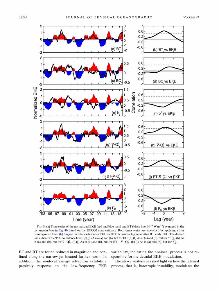
c. Temporal evolution

To clarify how the regional EKE modulates with the

barotropic instability, the area-averaged EKE and BT

over the largest EKE variance region (see the rectangle

box in Fig. 4b) is displayed in Fig. 8. Both time series are

low-pass filtered to highlight the interannual-to-decadal

variabilities. The EKE time series exhibits nearly simul-

taneous positive correlation (r5 0.64) with the BT, which

is statistically significant at the 95% confidence level

(critical value r0 5 0.45) by the Student’s t test. The

number of degrees of freedom for the low-pass filtered

EKE time series is estimated at 17 from its decorrelation

time scale. The low-pass time series of area-averagedBC,

b1, and = �Q1

* are also plotted in Fig. 8. The figure shows

the BC is not significantly correlated with the EKE (r 50.31 when BC leads EKE by ;5 months), and the

buoyancy conversion is negatively correlated with EKE

(r 5 20.32 with no apparent phase lag), indicating that

the baroclinic pathway breaks down at low frequencies

due to insignificant phase correlations betweenBCand b1

. In addition, the nonlocal term = �Q1

* and EKE are

found positively correlated with a synchronous correla-

tion coefficient of 0.55, indicating that the more EKE is

generated, the more is being carried away from this re-

gion. To make sure the EKE generated through baro-

tropic instability is accumulated within the upstream box,

we plot the area-averaged BT2= �Q1

* time series in

Fig. 8i. The figure shows a nearly simultaneous positive

correlation coefficient of 0.46 (statistically significant at a

95% confidence level), demonstrating that the EKE

generated by BT is indeed responsible for the decadal

EKE variability in this region. To see whether the above

energetics are well balanced in terms of the temporal

change of EKE, we plot the residue F1K series in Fig. 8k,

which includes all the external forcing and internal dis-

sipation processes. This residue term appears to be

smaller than the dominant BT term by one order of

magnitude, consistent with previous studies (Delman

et al. 2015). The negative sign, small magnitude (Fig. 8k),

and phase lag (Fig. 8l) indicate that the dissipation of

EKE is more important than the local external forcing in

the Kuroshio Extension. Besides, the small amplitude

also indicates that the EKE energetics are overall

balanced.

The temporal energetics results shown above clearly

demonstrate that the barotropic instability is the

dominant process for the decadal EKE modulations

detected in the upstream Kuroshio Extension. As is

shown in section 4a, the enhanced nonzonal meander-

ing plays an important role to induce enhanced baro-

tropic instability. Notice that the explanation for the

time–lag between the low-pass transfer rate (i.e., BT

and BC) and EKE is not trivial because eddies with

long lifespan may survive more than 1 year and leave

their imprints on the regional EKE and eddy–mean

flow interactions on interannual time scales (Chang and

Oey 2014). The exact eddy growth rate due to baro-

tropic and baroclinic instabilities should be carefully

examined, and we leave that to future studies.

5. Summary and discussion

Using the outputs from a dynamically consistent

global eddying state estimate, the localized multiscale

energy and vorticity analysis [MS-EVA; Liang and

Robinson 2005, 2007; a comprehensive development is

referred to Liang (2016)] was employed to investigate

the mechanism of the decadal EKE variability in the

upstream Kuroshio Extension region. We first used a

new functional analysis tool (MWT; Liang and

Anderson 2007) to decompose the associated fields

into a slow, modulating mean flow component and a

transient eddy component, instead of simply separating

them into a timemean and its deviation. In this way, the

low-frequency variability of the background jet is

largely retained in the mean flow window, which is es-

sential to investigate the time-varying diagram of the

eddy–mean flow interactions and instabilities un-

derlying the decadally modulating Kuroshio Extension

system. Besides, the orthogonality between the result-

ing scale windows allows for a faithful representation of

the eddy energetics.

The resulting energy maps and temporal series all

demonstrate that barotropic instability is the primary

source for the decadal EKE variability. The meanders

have been found responsible for the generation of

EKE in the upstream region. When the jet is weak, the

meander of the upstream Kuroshio Extension jet is

strong, which enhances both the barotropic transfer

from MKE to EKE and baroclinic transfer from

MAPE to EAPE. However, strong EAPE gained from

the MAPE reservoir through the baroclinic instability

process does not lead to increased EKE due to in-

sufficient in-phase conversion from EAPE to EKE. In

contrast, the growing meander induces significant

barotropic instability, which efficiently releases energy

from MKE to EKE, resulting in increased eddy activ-

ities in the upstream as the Kuroshio Extension is in

the high-EKE state. During the low-EKE state, both

MAY 2017 YANG ET AL . 1179

BC and BT are found reduced in magnitude and con-

fined along the narrow jet located farther north. In

addition, the nonlocal energy advection exhibits a

passively response to the low-frequency EKE

variability, indicating the nonlocal process is not re-

sponsible for the decadal EKE modulation.

The above analysis has shed light on how the internal

process, that is, barotropic instability, modulates the

FIG. 8. (a) Time series of the normalized EKE (red and blue bars) and BT (black line; 1024Wm23) averaged in the

rectangular box in Fig. 4b based on the ECCO2 state estimate. Both times series are smoothed by applying a 1-yr

runningmean filter. (b) Lagged correlation betweenEKEandBT.Apositive lagmeans thatBT leadsEKE.The dashed

line indicates the 95%confidence level. (c),(d)As in (a) and (b), but forBC. (e),(f)As in (a) and (b), but forb1. (g),(h)As

in (a) and (b), but for = �Q1

*. (i),(j) As in (a) and (b), but for BT2= �Q1

*. (k),(l) As in (a) and (b), but for F1K .

1180 JOURNAL OF PHYS ICAL OCEANOGRAPHY VOLUME 47

low-frequency EKE variation. It is natural to ask what

mechanism might trigger such an internal oscillation. Is

it externally forced or purely intrinsic? By analyzing the

available sea surface height (SSH) data from the mul-

tiple satellite altimeters from 1993 to 2005, Qiu and

Chen (2005) suggested that a meandering (straight) jet

path of the Kuroshio Extension is induced by the

southward (northward) migration of the inflow jet,

which rides over a shallow (deep) segment of the Izu–

Ogasawara Ridge. The southward (northward) migra-

tion of the jet is believed to be forced by the impinging

negative (positive) SSH anomalies via the westward

propagation of baroclinic Rossby waves generated in the

central North Pacific (Qiu 2003; Ceballos et al. 2009;

Nakano and Ishikawa 2010; Sasaki and Schneider 2011).

Instead, some studies reported that changes in the

meandering state of the Kuroshio Extension are related

to the path of the Kuroshio south of Japan; a meander-

ing (straight) jet path was associated with the Kuroshio

taking the offshore nonlarge (nearshore nonlarge or

typical large) meander path (Sugimoto and Hanawa

2012; Seo et al. 2014). As models have shown that the

bimodality of the Kuroshio path south of Japan have a

predominant intrinsic origin (Qiu and Miao 2000),

Sugimoto and Hanawa (2012) argued that the meander-

ing state of the Kuroshio Extension is not directly caused

by the external Rossby waves.

Although no consensus has been reached so far, it is

important to explore whether the aforementioned BT is

related to the large-scale wind variability in the eastern

basin. Previous studies have robust evidence of the

Kuroshio Extension’s response to the anomalous wind

stress curl generated in the central North Pacific with a

delay of a few years through westward propagation of

baroclinic Rossby waves (Deser et al. 1999; Qiu 2003).

Several recent studies have shown both the Pacific de-

cadal oscillation (PDO) and the North Pacific Gyre

Oscillation (NPGO) are good indicators for the decadal

changes of Kuroshio Extension because the two modes

are linearly correlated during the last two decades (Qiu

and Chen 2010; Qiu et al. 2015). In the following, we

choose the NPGO index to see whether it leaves any

footprints in the internal dynamics underlying the

Kuroshio Extension. The NPGO is an oceanic expres-

sion of the North Pacific Oscillation (NPO), defined by

the PC-2 of SSH anomaly in the northeastern Pacific

region 258–628N, 1808–1108W (Fig. 9a; Di Lorenzo et al.

2008; Ceballos et al. 2009). The spatial pattern of the

NPGO reveals a clear dipole structure both in the pro-

jections of wind stress vector and SSH anomaly in the

eastern and central North Pacific, as shown in Fig. 9b.

Dynamically, the anomalous negative wind stress curl

during the positive phase of NPGO over the subtropical

gyre forces an anomalous positive SSH anomaly through

local Ekman convergence. The wind-induced anomalous

SSH signals then propagate westward into the upstream

Kuroshio Extension after a delay of approximately 2

years, causing the regional SSH to change (Fig. 9c).

FIG. 9. (a) NPGO index. (b) Spatial correlation pattern between

NPGO and surface wind stress from ECCO2 (vectors) and be-

tween NPGO and SSH anomaly fromECCO2 (colored shading) at

0-yr lag. (c) Time–longitude diagram of the lagged correlation

between NPGO and SSH anomaly along the 318–368N band. A

positive lag indicates that NPGO takes the lead. The annual cycle

of the SSH anomaly is removed before processing the analysis.

FIG. 10. Lagged correlation between the negative NPGOand the

EKE time series (black) and between the negative NPGO and BT

time series (dotted) integrated in the rectangle box in Fig. 4b. A

positive lag indicates that NPGO takes the lead.

MAY 2017 YANG ET AL . 1181

Figure 10 shows that the upstream BT is positively

correlated with the negative NPGO index, with a cor-

relation coefficient of 0.45 when the NPGO leads BT by

;2 yr. The above results indicate that the internal pro-

cess that gives rise to the decadal EKEmodulation in the

upstream Kuroshio Extension is moderately correlated

to the anomalous wind stress curl generated in the

central North Pacific. Besides, the time lag also seems to

be in agreement with the time period of the baroclinic

adjustment in the North Pacific Ocean (Ceballos et al.

2009). Based on an eddy-resolving OGCM, Taguchi

et al. (2007) suggested that the intrinsic nonlinear be-

havior of the Kuroshio Extension could be possibly ex-

cited by the externally generated baroclinic Rossby

waves, but they did not provide a dynamical explana-

tion. Using a simple shallow-water model, Pierini (2014)

also showed a case of intrinsic variability in an excitable

dynamical system triggered by the North Pacific Oscil-

lation forcing. Consistent with Taguchi et al. (2007) and

Pierini (2014), our preliminary results also suggest that

an important fraction of the internal barotropic instability

is forced and deterministic in nature. Nevertheless, a

complete story is by no means an easy task in the Kur-

oshio Extension due to the varying external and internal

forcings, and the potential nonlinear interplay between

the two. Remote atmospheric forcing, the upstream

Kuroshio inflow, the underlying bathymetry, and frontal

nonlinear processes all need to be taken into account for a

faithful understanding of the complex dynamics in this

region. Further studies are needed to clarify how these

individual processes as well as their mutual interactions

might contribute to the decadal variability of the Kur-

oshio Extension and its associated eddies.

Acknowledgments. We appreciate Emanuele Di

Lorenzo’s important suggestions. Thanks are also due to

an anonymous reviewer for his comments. Yang Yang

thanks Andrew S. Delman for sharing the jet reference

frame algorithm. The ECCO2 datasets are available

from the site of the Jet Propulsion Laboratory, Cal-

ifornia Institute of Technology (http://ecco2.jpl.nasa.

gov/), and the NPGO index is available online (at http://

eros.eas.gatech.edu/npgo/data/NPGO.txt; the MS-EVA

software is available at http://www.ncoads.org/). This

work was supported by the National Science Foun-

dation of China (NSFC) under Grant 41276032, by the

Jiangsu Provincial Government through the Jiangsu

Chair Professorship and the 2015 Jiangsu Program of

Entrepreneurship and Innovation Group, and by the

State Oceanic Administration through the National

Program on Global Change and Air-Sea Interaction

(GASI-IPOVAI-06). BQ and SC acknowledge sup-

port from NSF OCE-0926594.

APPENDIX

Justification for the Dataset Selection

Area-mean (within the gray box in Fig. 4b) surface

EKE density series from three different model outputs,

namely, the ECCO2 state estimate, Japan Coastal

Ocean Predictability Experiment 2 (JCOPE2) re-

analysis, and the OGCM for the Earth Simulator

(OFES) hindcast are shown here to see to what degree

thesemodeling products fit in for our purpose in terms of

the reproducibility of the decadal EKE variability in the

Kuroshio Extension region.

The OFES is based on the Modular Ocean Model,

version 3 (MOM3) with no observational data assimi-

lated (Masumoto et al. 2004). Although several previous

studies reported that the OFES data successfully re-

produced the decadal SSH variability observed by sat-

ellite observations (Taguchi et al. 2007; Ceballos et al.

2009), the regional EKE level is largely biased

(Fig. A1d; Table A1). Based on the Princeton Ocean

Model (POM) and combined with the 3D variational

FIG. A1. Area-mean surface EKE time series (averaged over the

rectangle box in Fig. 4b) constructed from (a) the satellite obser-

vation (AVISO), (b) the ECCO2 state estimate, (c) the JCOPE2

reanalysis, and (d) the OFES hindcast.

1182 JOURNAL OF PHYS ICAL OCEANOGRAPHY VOLUME 47

method to assimilate satellite observations and

temperature–salinity profiles, the JCOPE2 reanalysis

(Miyazawa et al. 2009) reproduced the observed EKE

variability to a high degree (Fig. A1c; Table A1). The

data assimilation is performed every 7 days to bring

the model ‘‘on track’’ by minimizing the misfit between

the model and the observation. Such an assimilation

scheme will inevitably introduce jumps and unphysical

sources/sinks that no longer satisfy the model equations

(Wunsch et al. 2009). Thus, themodel output may not be

dynamically consistent and therefore may not be ap-

propriate for eddy energetics analysis. In contrast, the

ECCO2 state estimate is optimized by the observation

by using aGreen’s function approach (Menemenlis et al.

2005). A least squares fit is employed for a number of

control parameters of the model, for example, the initial

temperature and salinity conditions, atmospheric sur-

face boundary conditions, background vertical diffusiv-

ity, bottom drag, vertical viscosity, and so on (Wunsch

et al. 2009). With these optimized control parameters,

the model is run forward freely, just as in any ordinary

model simulation. Since no data are taken in to interrupt

the forward run, the state estimate is dynamically and

kinematically consistent, without introducing non-

physical jumps and artificial imbalances in the numerical

solution (Wunsch et al. 2009). To further check whether

FIG. A2. (a) Monthly time series of the zonal wind stress from the NCEP reanalysis (red) and the ECCO2 state

estimate (blue) averaged over the rectangle box in Fig. 4b. The dotted line denotes the difference between the two

datasets. (b) Lagged correlation between the zonal wind stress from the NCEP reanalysis and the EKE time series

(red line) and between the zonal wind stress from the ECCO2 state estimate and the EKE time series (blue line). A

positive lag indicates that the zonal wind stress takes lead. The dashed lines indicate the 95% confidence level.

(c),(d) As in (a) and (b), but for the meridional wind stress. (e),(f) As in (a) and (b), but for the surface heat flux.

TABLE A1. Different datasets and the correlation between the area-mean EKE time series from these datasets and that from the satellite

observation (AVISO).

Dataset Optimization method Correlation with AVISO series

ECCO2 Green function method (Menemenlis et al. 2005); no data taken in during forward run 0.64

JCOPE2 3D variational data assimilation (Miyazawa et al. 2009) 0.93

OFES No data assimilated 20.20

MAY 2017 YANG ET AL . 1183

the corrected surface boundary conditions (one of the

control parameters) in the ECCO2 state estimates could

impact the overall energetics, we plot the correlations

between the EKE and ECCO2 as well as the NCEP

surface fluxes averaged over our research box in Fig. A2.

Although there exist noticeable differences (Figs. A2a,c,e),

the correlations between the corrected surface fluxes

and the model EKE are almost identical to the ones

between theNCEP fluxes and the EKE (see the lead–lag

correlations in Figs. A2b,d,f). Besides, the correlations

between the local atmosphere forcings and the regional

EKE are small, and, actually, they are far below signif-

icant. To see whether these surface fluxes and the EKE

are correlated on the interannual-to-decadal time scale,

we also plot the lead–lag correlations between the cor-

responding low-pass time series in Figs. A3a–c. Again,

neither the wind stress nor the heat flux is significantly

correlated with the associated EKE. (They are not

statistically significant at both the 90% and 95% con-

fidence level.) In fact, in this region, it is the ocean-

to-atmosphere forcing that dominates the air–sea

interaction, as reported previously (e.g., Nonaka and

Xie 2003; Qiu et al. 2014; Seo et al. 2014). Here, the local

heat flux is weakly and negatively correlated with the

EKE (r 5 20.22), which is consistent with previous

findings that during the high-EKE state, the upper ocean

releases more heat to the overlying atmosphere due to

strengthened activities of the anticyclonic (warm) eddies

detached from the Kuroshio Extension (Sugimoto and

Hanawa 2011). To further check whether the corrected

heat flux would impact the regional eddy activity

through baroclinic instability processes, we plot the

correlation between the heat flux and the buoyancy

conversion term b1 (i.e., EAPE / EKE) in Fig. A3d.

Again, the lead–lag correlations are not significant.

Moreover, these two processes are not correlated at lag

0, implying that the surface buoyancy forcing has no

direct contributions to the generation of EKE at this

region. The above results indicate that the assimilation

scheme employed in the ECCO2 state estimate is not

FIG. A3. (a) Lagged correlation between the corrected zonal wind stress averaged over the rectangle box in

Fig. 4b and the EKE time series. All times series are smoothed by applying a 1-yr runningmean filter. A positive lag

indicates that the wind stress takes the lead. (b)As in (a), but for themeridional wind stress. (c) As in (a), but for the

net heat flux. (d) The lagged correlation between the net heat flux and the buoyancy conversion. The long (short)

dashed lines indicate the 90% (95%) confidence level.

1184 JOURNAL OF PHYS ICAL OCEANOGRAPHY VOLUME 47

likely to significantly affect the modeled EKE by cor-

recting the local atmosphere forcings. Thus, we can

safely conclude that the ECCO2 solution is appropriate

for the diagnosis of ocean budgets. Figure A1b shows

the area-mean EKE of the upstream Kuroshio Exten-

sion from the ECCO2 output. Obviously, the ECCO2

properly reproduced the two complete cycles of the

decadal EKE variability in the upstream Kuroshio Ex-

tension region. For all the above reasons, we choose the

ECCO2 state estimate as the input of the time-varying

MS-EVA application, even though the correlation be-

tween ECCO2 and the satellite data is not as high as that

between the JCOPE2 reanalysis and the satellite data

(Table A1).

REFERENCES

Abernathey, R., and P. Cessi, 2014: Topographic enhancement of

eddy efficiency in baroclinic equilibration. J. Phys. Oceanogr.,

44, 2107–2126, doi:10.1175/JPO-D-14-0014.1.

Berloff, P., A. M. C. Hogg, and W. Dewar, 2007: The turbulent

oscillator: A mechanism of low-frequency variability of the

wind-driven ocean gyres. J. Phys. Oceanogr., 37, 2363–2386,

doi:10.1175/JPO3118.1.

Bischoff, T., and A. F. Thompson, 2014: Configuration of a

Southern Ocean storm track. J. Phys. Oceanogr., 44, 3072–

3078, doi:10.1175/JPO-D-14-0062.1.

Bishop, S. P., 2013: Divergent eddy heat fluxes in the Kuroshio

Extension at 1448–1488E. Part II: Spatiotemporal variabil-

ity. J. Phys. Oceanogr., 43, 2416–2431, doi:10.1175/

JPO-D-13-061.1.

Cai, M., S. Yang, H. M. Van Den Dool, and V. E. Kousky, 2007:

Dynamical implications of the orientation of atmospheric

eddies: A local energetics perspective. Tellus, 59A, 127–140,

doi:10.1111/j.1600-0870.2006.00213.x.

Ceballos, L. I., E. Di Lorenzo, C. D. Hoyos, N. Schneider, and

B. Taguchi, 2009: North Pacific Gyre Oscillation synchronizes

climate fluctuations in the eastern and western boundary sys-

tems. J. Climate, 22, 5163–5174, doi:10.1175/2009JCLI2848.1.

Chang, E. K. M., 2001: GCM and observational diagnoses of the

seasonal and interannual variations of the Pacific storm track

during the cool season. J. Atmos. Sci., 58, 1784–1800,

doi:10.1175/1520-0469(2001)058,1784:GAODOT.2.0.CO;2.

Chang, Y.-L., and L.-Y. Oey, 2014: Instability of the North Pacific

Subtropical Countercurrent. J. Phys. Oceanogr., 44, 818–833,

doi:10.1175/JPO-D-13-0162.1.

Chapman, C. C., A. M. Hogg, A. E. Kiss, and S. R. Rintoul, 2015:

The dynamics of Southern Ocean storm tracks. J. Phys. Oce-

anogr., 45, 884–903, doi:10.1175/JPO-D-14-0075.1.

Chen, R., A. F. Thompson, andG. R. Flierl, 2016: Time-dependent

eddy-mean energy diagrams and their application to the

ocean. J. Phys. Oceanogr., 46, 2827–2850, doi:10.1175/

JPO-D-16-0012.1.

Chen, X., B. Qiu, S. Chen, Y. Qi, and Y. Du, 2015: Seasonal eddy

kinetic energy modulations along the North Equatorial

Countercurrent in the western Pacific. J. Geophys. Res.

Oceans, 120, 6351–6362, doi:10.1002/2015JC011054.

Chiba, S., E. Di Lorenzo, A. Davis, J. E. Keister, B. Taguchi, Y. Sasai,

and H. Sugisaki, 2013: Large-scale climate control of zooplank-

ton transport and biogeography in the Kuroshio-Oyashio

Extension region. Geophys. Res. Lett., 40, 5182–5187,

doi:10.1002/grl.50999.

Delman, A. S., J. L.McClean, J. Sprintall, L. D. Talley, E. Yulaeva,

and S. R. Jayne, 2015: Effects of eddy vorticity forcing on the

mean state of the Kuroshio Extension. J. Phys. Oceanogr., 45,

1356–1375, doi:10.1175/JPO-D-13-0259.1.

Deser, C., M. A. Alexander, andM. S. Timlin, 1999: Evidence for a

wind-driven intensification of theKuroshioCurrent Extension

from the 1970s to the 1980s. J. Climate, 12, 1697–1706,

doi:10.1175/1520-0442(1999)012,1697:EFAWDI.2.0.CO;2.

Di Lorenzo, E., and Coauthors, 2008: North Pacific Gyre Oscilla-

tion links ocean climate and ecosystem change.Geophys. Res.

Lett., 35, L08607, doi:10.1029/2007GL032838.

Ducet, N., P. Y. Le Traon, and G. Reverdin, 2000: Global high-

resolution mapping of ocean circulation from TOPEX/

Poseidon and ERS-1 and -2. J. Geophys. Res., 105, 19 477–

19 498, doi:10.1029/2000JC900063.

Elipot, S., and L. M. Beal, 2015: Characteristics, energetics, and

origins of Agulhas Current meanders and their limited influ-

ence on ring shedding. J. Phys. Oceanogr., 45, 2294–2314,

doi:10.1175/JPO-D-14-0254.1.

Ferrari, R., and C.Wunsch, 2009: Ocean circulation kinetic energy:

Reservoirs, sources, and sinks. Annu. Rev. Fluid Mech., 41,

253–282, doi:10.1146/annurev.fluid.40.111406.102139.

Frankignoul, C., and P. Müller, 1979: Quasi-geostrophic response

of an infinite b-plane ocean to stochastic forcing by the at-

mosphere. J. Phys. Oceanogr., 9, 104–127, doi:10.1175/

1520-0485(1979)009,0104:QGROAI.2.0.CO;2.

Fu, L.-L., 2009: Pattern and velocity of propagation of the global

ocean eddy variability. J. Geophys. Res., 114, C11017,

doi:10.1029/2009JC005349.

Garnier, V., and R. Schopp, 1999:Wind influence on the mesoscale

activity along the Gulf Stream and the North Atlantic cur-

rents. J. Geophys. Res., 104, 18 087–18 110, doi:10.1029/

1999JC900070.

Gill, A. E., J. S. A. Green, and A. J. Simmons, 1974: Energy par-

tition in the large-scale ocean circulation and the production

of mid-ocean eddies.Deep-Sea Res. Oceanogr. Abstr., 21, 499–

528, doi:10.1016/0011-7471(74)90010-2.

Grooms, I., L.-P. Nadeau, and K. S. Smith, 2013: Mesoscale eddy

energy locality in an idealized ocean model. J. Phys. Ocean-

ogr., 43, 1911–1923, doi:10.1175/JPO-D-13-036.1.

Hall, M. M., 1991: Energetics of the Kuroshio Extension at

358N, 1528E. J. Phys. Oceanogr., 21, 958–975, doi:10.1175/

1520-0485(1991)021,0958:EOTKEA.2.0.CO;2.

Hogg, A. M. C., P. D. Killworth, J. R. Blundell, and W. K. Dewar,

2005: Mechanisms of decadal variability of the wind-driven

ocean circulation. J. Phys. Oceanogr., 35, 512–531,

doi:10.1175/JPO2687.1.

Itoh, S., and I. Yasuda, 2010: Characteristics of mesoscale eddies in

the Kuroshio–Oyashio Extension region detected from the

distribution of the sea surface height anomaly. J. Phys. Oce-

anogr., 40, 1018–1034, doi:10.1175/2009JPO4265.1.

Jia, F., L. Wu, J. Lan, and B. Qiu, 2011: Interannual modulation of

eddy kinetic energy in the southeast IndianOcean by southern

annular mode. J. Geophys. Res., 116, C02029, doi:10.1029/

2010JC006699.

Kang, D., E. N. Curchitser, and A. Rosati, 2016: Seasonal vari-

ability of the Gulf Stream kinetic energy. J. Phys. Oceanogr.,

46, 1189–1207, doi:10.1175/JPO-D-15-0235.1.

Kida, S., and Coauthors, 2015: Oceanic fronts and jets around Ja-

pan: A review. J. Oceanogr., 71, 469–497, doi:10.1007/

s10872-015-0283-7.

MAY 2017 YANG ET AL . 1185

Kwon, Y.-O., and C. Deser, 2007: North Pacific decadal variability

in the Community Climate System Model version 2.

J. Climate, 20, 2416–2433, doi:10.1175/JCLI4103.1.

Latif, M., and T. P. Barnett, 1994: Causes of decadal climate vari-

ability over theNorth Pacific andNorthAmerica. Science, 266,

634–637, doi:10.1126/science.266.5185.634.

Liang, X. S., 2016: Canonical transfer and multiscale energetics for

primitive and quasigeostrophic atmospheres. J. Atmos. Sci.,

73, 4439–4468, doi:10.1175/JAS-D-16-0131.1.

——, and A. R. Robinson, 2005: Localized multiscale energy and

vorticity analysis: I. Fundamentals. Dyn. Atmos. Oceans, 38,

195–230, doi:10.1016/j.dynatmoce.2004.12.004.

——, andD. G.M.Anderson, 2007:Multiscale window transform.

Multiscale Model. Simul., 6, 437–467, doi:10.1137/

06066895X.

——, and A. R. Robinson, 2007: Localized multi-scale energy

and vorticity analysis: II. Finite-amplitude instability theory

and validation.Dyn. Atmos. Oceans, 44, 51–76, doi:10.1016/

j.dynatmoce.2007.04.001.

——, and——, 2009: Multiscale processes and nonlinear dynamics

of the circulation and upwelling events off Monterey Bay.

J. Phys. Oceanogr., 39, 290–313, doi:10.1175/2008JPO3950.1.

Lorenz, E. N., 1955: Available potential energy and the mainte-

nance of the general circulation. Tellus, 7, 157–167,

doi:10.3402/tellusa.v7i2.8796.

Marshall, J., A. Adcroft, C. Hill, L. Perelman, and C. Heisey, 1997:

A finite-volume, incompressible Navier Stokes model for

studies of the ocean on parallel computers. J. Geophys. Res.,

102, 5753–5766, doi:10.1029/96JC02775.

Masumoto, Y., and Coauthors, 2004: A fifty-year eddy-resolving

simulation of the world ocean: Preliminary outcomes of OFES

(OGCM for the Earth Simulator). J. Earth Simul., 1, 35–56.

McCalpin, J. D., andD. B. Haidvogel, 1996: Phenomenology of the

low-frequency variability in a reduced-gravity, quasigeo-

strophic double-gyre model. J. Phys. Oceanogr., 26, 739–752,

doi:10.1175/1520-0485(1996)026,0739:POTLFV.2.0.CO;2.

Menemenlis, D., I. Fukumori, and T. Lee, 2005: Using Green’s

functions to calibrate an ocean general circulation model.

Mon. Wea. Rev., 133, 1224–1240, doi:10.1175/MWR2912.1.

Miller, A. J., D. R. Cayan, and W. B. White, 1998: A westward-

intensified decadal change in the North Pacific thermocline

and gyre-scale circulation. J. Climate, 11, 3112–3127,

doi:10.1175/1520-0442(1998)011,3112:AWIDCI.2.0.CO;2.

——, F. Chai, S. Chiba, J. R. Moisan, and D. J. Neilson, 2004:

Decadal-scale climate and ecosystem interactions in the

North Pacific Ocean. J. Oceanogr., 60, 163–188, doi:10.1023/

B:JOCE.0000038325.36306.95.

Miyazawa, Y., and Coauthors, 2009: Water mass variability in the

western North Pacific detected in a 15-year eddy resolving

ocean reanalysis. J. Oceanogr., 65, 737, doi:10.1007/

s10872-009-0063-3.

Mizuno, K., and W. B. White, 1983: Annual and interannual

variability in the Kuroshio Current System. J. Phys. Ocean-

ogr., 13, 1847–1867, doi:10.1175/1520-0485(1983)013,1847:

AAIVIT.2.0.CO;2.

Müller, P., and C. Frankignoul, 1981: Direct atmospheric forcing of

geostrophic eddies. J. Phys. Oceanogr., 11, 287–308,

doi:10.1175/1520-0485(1981)011,0287:DAFOGE.2.0.CO;2.

Nakamura, H., T. Izumi, and T. Sampe, 2002: Interannual and

decadal modulations recently observed in the Pacific storm

track activity and East Asian winter monsoon. J. Climate,

15, 1855–1874, doi:10.1175/1520-0442(2002)015,1855:

IADMRO.2.0.CO;2.

Nakano,H., and I. Ishikawa, 2010:Meridional shift of theKuroshio

Extension induced by response of recirculation gyre to de-

cadal wind variations. Deep-Sea Res. II, 57, 1111–1126,

doi:10.1016/j.dsr2.2009.12.002.

Nishikawa,H., and I. Yasuda, 2011: Long-term variability of winter

mixed layer depth and temperature along the Kuroshio jet in a

high-resolution ocean general circulationmodel. J. Oceanogr.,

67, 503–518, doi:10.1007/s10872-011-0053-0.

Nonaka, M., and S.-P. Xie, 2003: Covariations of sea surface

temperature and wind over the Kuroshio and its extension:

Evidence for ocean-to-atmosphere feedback. J. Climate,

16, 1404–1413, doi:10.1175/1520-0442(2003)16,1404:

COSSTA.2.0.CO;2.

——, H. Nakamura, Y. Tanimoto, T. Kagimoto, and H. Sasaki,

2006: Decadal variability in the Kuroshio–Oyashio Extension

simulated in an eddy-resolving OGCM. J. Climate, 19, 1970–

1989, doi:10.1175/JCLI3793.1.

O’Reilly, C. H., and A. Czaja, 2015: The response of the Pacific

storm track and atmospheric circulation to Kuroshio Exten-

sion variability. Quart. J. Roy. Meteor. Soc., 141, 52–66,

doi:10.1002/qj.2334.

Pedlosky, J., 1987:Geophysical Fluid Dynamics. 2nd ed. Springer-

Verlag, 710 pp.

Penduff, T., B. Barnier, W. K. Dewar, and J. J. O’Brien, 2004:

Dynamical response of the oceanic eddy field to the North

Atlantic Oscillation: A model–data comparison. J. Phys.

Oceanogr., 34, 2615–2629, doi:10.1175/JPO2618.1.

Pierini, S., 2014: Kuroshio Extension bimodality and the North

Pacific Oscillation: A case of intrinsic variability paced by

external forcing. J. Climate, 27, 448–454, doi:10.1175/

JCLI-D-13-00306.1.

——,H.A.Dijkstra, andA. Riccio, 2009: A nonlinear theory of the

Kuroshio Extension bimodality. J. Phys. Oceanogr., 39, 2212–

2229, doi:10.1175/2009JPO4181.1.

Primeau, F., and D. Newman, 2008: Elongation and contraction of

the western boundary current extension in a shallow-water

model: A bifurcation analysis. J. Phys. Oceanogr., 38, 1469–

1485, doi:10.1175/2007JPO3658.1.

Qiu, B., 2003: Kuroshio extension variability and forcing of the

Pacific decadal oscillations: Responses and potential feed-

back. J. Phys. Oceanogr., 33, 2465–2482, doi:10.1175/2459.1.

——, and W. Miao, 2000: Kuroshio path variations south of Japan:

Bimodality as a self-sustained internal oscillation. J. Phys. Oce-

anogr., 30, 2124–2137, doi:10.1175/1520-0485(2000)030,2124:

KPVSOJ.2.0.CO;2.

——, and S. Chen, 2005: Variability of the Kuroshio Extension jet,

recirculation gyre, and mesoscale eddies on decadal time

scales. J. Phys. Oceanogr., 35, 2090–2103, doi:10.1175/

JPO2807.1.

——, and ——, 2010: Eddy-mean flow interaction in the decadally

modulating Kuroshio Extension system. Deep-Sea Res. II, 57,

1098–1110, doi:10.1016/j.dsr2.2008.11.036.

——, and ——, 2013: Concurrent decadal mesoscale eddy modu-

lations in the western North Pacific Subtropical Gyre. J. Phys.

Oceanogr., 43, 344–358, doi:10.1175/JPO-D-12-0133.1.

——,——, P.Hacker, N.G.Hogg, S. R. Jayne, andH. Sasaki, 2008:

The Kuroshio Extension Northern Recirculation Gyre: Pro-

filing float measurements and forcing mechanism. J. Phys.

Oceanogr., 38, 1764–1779, doi:10.1175/2008JPO3921.1.

——, ——, N. Schneider, and B. Taguchi, 2014: A coupled de-

cadal prediction of the dynamic state of the Kuroshio Ex-

tension system. J. Climate, 27, 1751–1764, doi:10.1175/

JCLI-D-13-00318.1.

1186 JOURNAL OF PHYS ICAL OCEANOGRAPHY VOLUME 47

——,——, L. Wu, and S. Kida, 2015: Wind- versus eddy-forced

regional sea level trends and variability in the North Pa-

cific Ocean. J. Climate, 28, 1561–1577, doi:10.1175/

JCLI-D-14-00479.1.

Rhines, P., 1977: The dynamics of unsteady currents. Marine

Modeling, E. D. Goldberg et al., Eds., The Sea—Ideas and

Observations on Progress in the Study of the Seas, Vol. 6, John

Wiley and Sons, 189–318.

Sasai, Y., K. J. Richards, A. Ishida, and H. Sasaki, 2010: Effects of

cyclonic mesoscale eddies on the marine ecosystem in the

Kuroshio Extension region using an eddy-resolving coupled

physical-biological model. Ocean Dyn., 60, 693–704,

doi:10.1007/s10236-010-0264-8.

Sasaki, Y. N., and N. Schneider, 2011: Decadal shifts of the

KuroshioExtension jet:Application of thin-jet theory. J. Phys.

Oceanogr., 41, 979–993, doi:10.1175/2011JPO4550.1.

Schneider, N., A. J. Miller, and D. W. Pierce, 2002: Anatomy of

North Pacific decadal variability. J. Climate, 15, 586–605,

doi:10.1175/1520-0442(2002)015,0586:AONPDV.2.0.CO;2.

Seager, R., Y. Kushnir, N. H. Naik, M. A. Cane, and J. Miller,

2001: Wind-driven shifts in the latitude of the Kuroshio–

Oyashio Extension and generation of SST anomalies on de-

cadal timescales. J. Climate, 14, 4249–4265, doi:10.1175/

1520-0442(2001)014,4249:WDSITL.2.0.CO;2.

Seo, Y., S. Sugimoto, and K. Hanawa, 2014: Long-term variations

of the Kuroshio Extension path in winter: Meridional move-

ment and path state change. J. Climate, 27, 5929–5940,

doi:10.1175/JCLI-D-13-00641.1.

Simonnet, E., and H. A. Dijkstra, 2002: Spontaneous generation of

low-frequency modes of variability in the wind-driven ocean

circulation. J. Phys. Oceanogr., 32, 1747–1762, doi:10.1175/

1520-0485(2002)032,1747:SGOLFM.2.0.CO;2.

Smith, K. S., 2007: Eddy amplitudes in baroclinic turbulence

driven by nonzonal mean flow: Shear dispersion of potential

vorticity. J. Phys. Oceanogr., 37, 1037–1050, doi:10.1175/

JPO3030.1.

Spall, M. A., 2000: Generation of strong mesoscale eddies by

weak ocean gyres. J. Mar. Res., 58, 97–116, doi:10.1357/

002224000321511214.

Stammer, D., and C. Wunsch, 1999: Temporal changes in eddy

energy of the oceans. Deep-Sea Res. II, 46, 77–108,

doi:10.1016/S0967-0645(98)00106-4.

Sugimoto, S., and K. Hanawa, 2011: Roles of SST anomalies on the

wintertime turbulent heat fluxes in the Kuroshio–Oyashio

confluence region: Influences of warm eddies detached from

the Kuroshio Extension. J. Climate, 24, 6551–6561,

doi:10.1175/2011JCLI4023.1.

——, and ——, 2012: Relationship between the path of the

Kuroshio in the south of Japan and the path of the Kuroshio

Extension in the east. J. Oceanogr., 68, 219–225, doi:10.1007/

s10872-011-0089-1.

Sun, Z., Z. Zhang, W. Zhao, and J. Tian, 2016: Interannual mod-

ulation of eddy kinetic energy in the northeastern South China

Sea as revealed by an eddy-resolvingOGCM. J. Geophys. Res.

Oceans, 121, 3190–3201, doi:10.1002/2015JC011497.Taguchi, B., S.-P. Xie, N. Schneider, M. Nonaka, H. Sasaki, and

Y. Sasai, 2007: Decadal variability of the Kuroshio Extension:

Observations and an eddy-resolving model hindcast.

J. Climate, 20, 2357–2377, doi:10.1175/JCLI4142.1.——, B. Qiu, M. Nonaka, H. Sasaki, S.-P. Xie, and N. Schneider,

2010: Decadal variability of the Kuroshio Extension: Meso-

scale eddies and recirculations. Ocean Dyn., 60, 673–691,

doi:10.1007/s10236-010-0295-1.

Volkov, D. L., and L.-L. Fu, 2011: Interannual variability of the

Azores Current strength and eddy energy in relation to at-

mospheric forcing. J. Geophys. Res., 116, C11011, doi:10.1029/2011JC007271.

von Storch, J.-S., C. Eden, I. Fast, H. Haak, D. Hernández-Deckers, E. Maier-Reimer, J. Marotzke, and D. Stammer,

2012: An estimate of the Lorenz energy cycle for the World

Ocean based on the STORM/NCEP simulation. J. Phys.

Oceanogr., 42, 2185–2205, doi:10.1175/JPO-D-12-079.1.

Wang, Y.-H., and W. T. Liu, 2015: Observational evidence of

frontal-scale atmospheric responses to Kuroshio Extension

variability. J. Climate, 28, 9459–9472, doi:10.1175/

JCLI-D-14-00829.1.

Waterman, S., N. G. Hogg, and S. R. Jayne, 2011: Eddy–mean flow

interaction in the Kuroshio Extension region. J. Phys. Oce-

anogr., 41, 1182–1208, doi:10.1175/2010JPO4564.1.

White, M. A., and K. J. Heywood, 1995: Seasonal and interannual

changes in the NorthAtlantic SubpolarGyre fromGeosat and

TOPEX/POSEIDONaltimetry. J. Geophys. Res., 100, 24 931–

24 941, doi:10.1029/95JC02123.

Wunsch, C., P. Heimbach, R. Ponte, and I. Fukumori, 2009: The

global general circulation of the ocean estimated by the

ECCO-consortium. Oceanography, 22, 88–103, doi:10.5670/

oceanog.2009.41.

Yang, H., L.Wu,H. Liu, and Y. Yu, 2013: Eddy energy sources and

sinks in the South China Sea. J. Geophys. Res. Oceans, 118,

4716–4726, doi:10.1002/jgrc.20343.

Yang, Y., and X. S. Liang, 2016: The instabilities and multiscale

energetics underlying the mean–interannual–eddy in-

teractions in the Kuroshio Extension region. J. Phys. Ocean-

ogr., 46, 1477–1494, doi:10.1175/JPO-D-15-0226.1.

Zemskova, V. E., B. L. White, and A. Scotti, 2015: Available po-

tential energy and the general circulation: Partitioning wind,

buoyancy forcing, and diapycnal mixing. J. Phys. Oceanogr.,

45, 1510–1531, doi:10.1175/JPO-D-14-0043.1.

Zhai, X., R. J. Greatbatch, and J.-D. Kohlmann, 2008: On the

seasonal variability of eddy kinetic energy in the Gulf

Stream region.Geophys. Res. Lett., 35, L24609, doi:10.1029/

2008GL036412.

MAY 2017 YANG ET AL . 1187