J. Phys. A: Math. Gen. 15 (1982) 3241-3253. Printed in Great Britain

On the computational complexity of Ising spin glass models

Francisco Barahona Departamento de MatemBticas, Universidad de Chile, Casilla 5272, Correo 3, Santiago, Chile

Received 17 September 1981, in final form 13 April 1982

Abstract. In a spin glass with Ising spins, the problems of computing the magnetic partition function and finding a ground state are studied. In a finite two-dimensional lattice these problems can be solved by algorithms that require a number of steps bounded by a polynomial function of the size of the lattice. In contrast to this fact, the same problems are shown to belong to the class of w-hard problems, both in the two-dimensional case within a magnetic field, and in the three-dimensional case. Np-hardness of a problem suggests that it is very unlikely that a polynomial algorithm could exist to solve it.

1. Introduction

The problem of spin glasses is of great interest both in solid state physics and in statistical physics. The materials studied are magnetic alloys such as 1% of magnetic impurities embedded in Cu or Au. A property of these systems is the cusp in the magnetic susceptibility at a well defined temperature, indicating a phase transition, but the question if there is another phase transition is not yet solved.

Between two impurities there is an energy interaction

H I Z = -J(rI2)S1 S2,

where Si is the magnetic moment (spin) of the impurity i, and the interaction J ( r ) varies as cos(2KFr)/r3, where r is the distance between the impurities, and KF a physical constant.

The energy of a spin configuration is given by the Hamiltonian

H = - C J ( rii)Si Si + 1 F * Si, where F is an exterior magnetic field.

The first step in modelling this problem is to substitute the random distribution of impurities by a disposition at the vertices of a regular lattice. The two-dimensional problem and the three-dimensional problem (written as 2D and 3D respectively) will be studied here.

The second step is to associate to each edge ( i , j ) of the lattice an interaction Ai chosen randomly from {-U, 0, U}.

Finally the three-dimensional vectors Si are replaced by one-dimensional vectors Si whose values can be *1 (Ising spins).

For a spin configuration w (an assignment of values f 1 to variables {Si}), the energy is given by

H ( w ) = -1 Ji$iSj +F 1 si.

0305-4470/82/103241+ 13$02.00 @ 1982 The Institute of Physics 3241

3242 F Barahona

It is believed that despite its strong simplifications, this model retains the relevant features of real spin glasses.

In this model two mathematical problems arise. The first is the study of the minimum energy configurations called ground states, and the second is the calculation of the magnetic partition function

f ( ~ ) = C exp[-H(w)/KTI, w € n

where i2 is the set of all spin configurations, H ( w ) is the energy of the configuration w, K is the Boltzmann constant, and T the temperature.

The free energy from the magnetic degree of freedom is -KT logf(T), and the equilibrium magnetic properties, magnetisation, entropy, magnetic energy, specific heat and susceptibility, can all be obtained by differentiating this function with respect to magnetic field and temperature.

The function f was obtained by Onsager (1944) for an infinite two-dimensional grid, but only when all interactions are equal to 1 (the ferromagnetic case), and without a magnetic field. The same information has since been obtained for other planar two-dimensional lattices, but a generalisation of these results for the three-dimensional lattice, or the two-dimensional lattice within a magnetic field or to the two-dimensional lattice with a more general distribution of the interactions, has been largely researched but not obtained..

The mathematical difficulty of these problems has led many researchers to carry out simulations utilising finite lattices, e.g. Barahona et a1 (1982), Bieche et a1 (1980), Binder (1975), Kirkpatrick (1977).

The study of finite lattices belongs to the field of algorithmic combinatorics. We will analyse their computational complexity in this paper.

In a grid with n spins, finding a ground state consists of searching for a spin configuration among 2” that minimises the energy. The partition function is a sum with 2” terms. For problems of this type there is a general agreement that if a problem cannot be solved in less than a number of calculations that grows exponentially with the size of the problem, then the problem should be considered completely intractable. On the other hand, it is accepted that a ‘good’ algorithm is an algorithm that requires a number of calculations bounded by a polynomial function of the size of the problem. In our case the size of the problem will be the number of spins.

In Fisher (1966) it has been shown that, for any planar lattice, the partition function can be computed by counting perfect matchings (dimers) in an expanded lattice. This can be accomplished in polynomial time by computing an appropriate Pfaffian (or determinant).

In Bieche et a1 (1980) the problem of getting a ground state is solved, in 2D, with a polynomial algorithm, by finding a minimum weighted perfect matching in the graph of ‘frustrated faces’.

In Barahona et a1 (1982) the morphology of the ground states has been studied with a related algorithm. This is done by obtaining the clusters of spins that have the same relative orientation in all ground states (clusters of ‘solidary spins’).

In 8 3 we will develop a unifying framework to solve, in polynomial time, for any planar lattice, the following problems: computing the partition function; finding a ground state; study of the morphology of the ground states; computing the entropy of the ground state.

This will be done by applying the matching theory (Cunningham 1978, Edmonds 1965, Edmonds and Johnson 1973, Kasteleyn 1961, 1967, Lawler 1976).

Computational complexity of Ising spin glass models 3243

After the results of Cook (1971) and Karp (1972), much work has been done to study the class of non-deterministic polynomial-time complete (NP-complete) prob- lems. This class includes many ‘classical’ problems in combinatorics, such as the travelling salesman problem, the Hamiltonian circuit problem, colourability of graphs, and integer linear programming, and all problems in the class have been shown to be ‘equivalent’, in the sense that if one problem is tractable, then all are. Since many of these problems have been studied by mathematicians and computer scientists for decades, and no good algorithm has been found for even one of them, it is natural to conjecture that no such polynomial algorithm exists. We will show that some spin glass models belong to this class. The interested reader is referred to Aho et a1 (1974) and Garey and Johnson (1979) for a review of the theory of NP-completeness.

In 0 4 we show that for both models, 2D within a magnetic field and 3D, there cannot exist a polynomial algorithm to compute the energy of the ground state (and the partition function), without the existence of a polynomial algorithm for all the NP-complete problems,

Some necessary graph theory definitions are given in § 2.

2. Definitions

In this section we summarise some basic definitions from graph theory, referring the reader to Berge (1970) and Harary (1969) for a more complete discussion.

A graph G = (V, E) consists of a set of vertices V, and a set E of unordered pairs of different vertices called edges. In our case vertices are associated with spins and edges with non-zero interactions. A chain between o1 and U, is a sequence of edges of the form (ut, v2) , (v2 , u ~ ) , . , . , U,). A cycle is a chain with u1 = up. To draw a graph we associate points to vertices and lines to edges. A graph is said to be embedded in a surface S when it is drawn on S so that no edges intersect. A graph is planar if it can be embedded in the plane, and a graph is toroidal if it can be embedded in a torus and not in the plane. For an embedded graph the regions defined by this embedding are called the faces. Given an embedded graph we define the geometric dual as follows: place a vertex in each face and, if two faces have an edge e in common, join the corresponding vertices by an edge e* crossing e.

Given two cycles C1 and C, we define Cl+C2 as the symmetrical difference between C1 and C2. A cycle generating family B is a set of cycles such that every cycle C can be expressed as C = C1 + C2 + . . . + Ck, with {Cl, . . . , Ck} E B. For planar graphs a cycle generating family are the faces. For toroidal graphs we have to add two cycles looping the torus. These cycles are essential and non-homologous.

For a graph G = (V, E) a perfect matching is a set M c E such that each vertex has only one edge of M adjacent to it.

An oriented graph is a graph G = (V, E) where E is a set of ordered pairs of vertices such that if ( i j ) E E then ( j , i) E! E. To an oriented graph we can associate a matrix B = [bi i ] , where

1 if ( i j ) E E b . .= -1 if ( j i ) E E ” L otherwise.

This matrix will be called the adjoint matrix of G. Kasteleyn (1961, 1967) has shown that, for plagar graphs, there exists an orienta-

tion of the edges such that the absolute value of the Pfaffian of B (Pf(B)) equals the

3244 F Barahona

number of perfect matchings of G, and furthermore, each non-vanishing term of Pf(B) corresponds to a perfect matching. As (Pf(B))’ = De@), the Pfaffian can be computed in polynomial time.

Given a graph G = (V, E ) and C c V we denote by S(C) the set of edges with exactly one extremity in C ; S(C) will be called a cocycle. A stable set S is a set of vertices such that if u and U belong to S then ( u u ) & E. The degree of a vertex is the number of edges adjacent to it. For a set S we will denote the cardinality of S by ISI.

3. The two-dimensional problem

3.1. Preliminaries

In this section we consider two types of grids, the planar 2D problem and the 2D problem with periodic boundary conditions. This last grid is a toroidal graph. Given a grid G = (V , E ) , to each vertex i is assigned a spin SI = *l , and to each edge ( i j ) is assigned an interaction JI,.

A spin configuration is an assignment of values *l to the variables {SI} . If all the signs of the variables {S,} are reversed, a new configuration is obtained which has the same energy as the former one. These pairs of spin configurations will be called pairs of equivalent configurations.

Given a pair of equivalent configurations an edge (ij) is satisfied if

Jil > 0 and S,SJ = 1, or JII < O and S,S, = -1,

For a cycle having an odd number of negative interactions there is no spin

The following two theorems are mentioned in Bieche et a1 (1980) and proved in

otherwise the edge is said to be unsatisfied.

configuration that satisfies all the edges. Such cycles are said to be frustrated.

Bieche (1979).

Theorem 1. There is a one-to-one correspondence between pairs of equivalent configurations and sets of unsatisfied edges verifying: (1) for every frustrated (unfrus- trated) cycle there is an odd (even) number of unsatisfied edges.

The following stronger theorem is more useful.

Theorem 2. There is a one-to-one correspondence between pairs of equivalent configurations and sets of unsatisfied edges verifying (1) for the elements of a cycle generating family.

Furthermore, given a pair of equivalent configurations it is easy to see that the energy can be expressed as follows.

(2) H = - 1 JlJSls, = - 1 IJIJ/ + 2 1 l J I J I *

lIJ)EE ( I J ) E E unsatisfied edges

3.2. The planar 2 0 problem

In this case, the faces form a cycle generating family. Then equivalent configurations

Computational complexity of Ising spin glass models 3245

are represented by sets of unsatisfied edges such that every frustrated (unfrustrated) face has an odd (even) number of those edges. Thus, if on each unsatisfied edge we draw a perpendicular line, a set of unsatisfied edges will be constituted by a set of chains joining pairs of frustrated faces and a set of closed polygons; see figure 1.

Figure 1. - Positive interaction, * Frustrated face, 7 Positive spin, - Negative interaction, - Unsatisfied edge, r( Negative spin.

This fact suggests to us to work in the dual graph G*. Vertices of G* will be called ‘odd’ and ‘even’ depending whether they represent a frustrated or unfrustrated face respectively. Odd (even) vertices must have an odd (even) number of unsatisfied edges adjacent to them.

Now we will describe how to transform G* in a graph d such that there is a one-to-one correspondence between configurations of unsatisfied edges in G* and perfect matchings in d. The first step of this transformation consists in expanding any vertex U of degree q > 3 in (q -- 2) copies of degree three as is shown in figure 2. If U is even, all its copies will be even. And if U is odd, one of them (arbitrarily) will be odd and all the others even.

Figure 2.

Now we will deal only with vertices of degree three. For an odd vertex of degree three we make the transformation schematised in figure 3.

Figure 3.

3246 F Barahona

Each configuration of unsatisfied edges corresponds to a perfect matching as is shown in figure 4.

Figure 4.

Even vertices of degree three are transformed as in figure 5 .

Figure 5.

Each configuration of unsatisfied edges is in correspondence with a perfect match- ing, see figure 6.

Figure 6.

To each edge e of d that represents an edge (ij) of the lattice G, the weight G ( e ) = lJiii is assigned. The weight G ( a ) of the other edges of d will be 0. We define the weight of a matching as the sum of the weights of edges in the matching.

By the transformations just described, it is clear that there is a one-to-one corres- pondence between pairs of equivalent configurations and perfect matchings in 6. If W is the weight of the matching, by equation ( 2 ) , the energy is

As the energy is a linear function of the weight of the matching, plus a constant, matching theory can be applied to solve the problems described below. Kasteleyn's procedure to count perfect matchings can be applied to compute the partition function. In the adjoint matrix B each coefficient with value *1 corresponding to the edge e is replaced by * x ~ ' ( ~ ) ; thus

Pf(B) = 1 UkX

where ak is the number of perfect matchings of weight k / 2 .

Computational complexity of Ising spin glass models 3247

Setting x = exp(-l/kT), and I = -Z(ij)EE IJijl, the partition function becomes

f [ T ( x ) ] = 2%’ Pf(B).

This procedure is polynomial because the Pfaffian of a matrix can be computed in polynomial time.

A ground state can be obtained by utilising Edmonds’ (1965) algorithm to find a minimum weighted perfect matching. If the primal algorithm for optimum matching (Cunningham 1978) is utilised, each change of the matching points out a cluster of spins that should be turned over to diminish the energy.

The knowledge of the structure of the ‘clusters of solidary spins’ can aid the study of the degeneracy of the ground state. Two spins are called solidary if they have the same relative orientation in all ground states. Clusters of solidary spins are joined by rigid edges. An edge is rigid if it is either satisfied or unsatisfied in all ground states.

Given a ground state (or a minimum weighted perfect matching in G), an edge e is rigid if:

(i) e belongs to the matching and any E > 0 that is added to @ ( e ) does not change the minimum weighted perfect matching;

(ii) e does not belong to the matching and any E > O that is subtracted from @(e) does not change the minimum weighted perfect matching.

The set of rigid edges can be determined efficiently with standard post-optimality procedures of linear programming (Dantzig 1962) and the primal algorithm for optimum matching (Cunningham 1978). The entropy of the ground state can be obtained in polynomial time by applying Kasteleyn’s procedure to count the minimum weighted perfect matchings in 6.

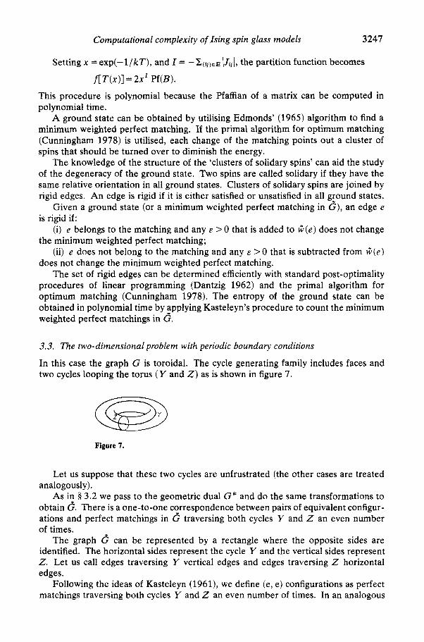
3.3. The two-dimensional problem with periodic boundary conditions

In this case the graph G is toroidal. The cycle generating family includes faces and two cycles looping the torus ( Y and 2) as is shown in figure 7.

Figure 7.

Let us suppose that these two cycles are unfrustrated (the other cases are treated analogously).

As in § 3.2 we pass to the geometric dual G* and do the same transformations to obtain 6. There is a one-to-one correspondence between pairs of equivalent configur- ations and perfect matchings in 6 traversing both cycles Y and 2 an even number of times.

The graph C? can be represented by a rectangle where the opposite sides are identified. The horizontal sides represent the cycle Y and the vertical sides represent 2. Let us call edges traversing Y vertical edges and edges traversing 2 horizontal edges.

Following the ideas of Kasteleyn (1961), we define (e, e) configurations as perfect matchings traversing both cycles Y and 2 an even number of times. In an analogous

3248 F Barahona

way we define (0, e), (e, 0) and (0, 0) configurations, where the first symbol refers to horizontal edges and the second to vertical edges, o means odd and e means even; see figure 8.

i e , e ) configurntion w io.el configurntion

1e.o) configuration io,ol configuration

Figure 8.

The graph e without the horizontal and vertical edges can be oriented as a planar graph. Then, horizontal edges are oriented regardless of vertical edges, and finally, vertical edges are oriented regardless of horizontal edges. We obtain an adjoint matrix B1 where Pf(Bl) counts only (e,e) configurations with the correct sign and all the others with the opposite sign. Then, three other adjoint matrices are defined:

B2 is obtained by reversing only vertical edges. B3 is obtained by reversing only horizontal edges. B4 is obtained by reversing both horizontal and vertical edges. Pf(B2) counts all configurations correctly except for the (0, e) configurations. Pf(B3) counts all configurations correctly except for the class (e, 0) and Pf(B4)

Utilising the definitions of § 3.2, the partition function can be written as counts all of them correctly except for those of type (0, 0).

f [ T ( X ) ] = 2X'i(-Pf(B1)+Pf(B*) +Pf(B,)+Pf(B4))

= x' (-Pf (B1) + Pf (B*) + Pf (B3) + Pf (B4)) *

4. NP-hard models

4.1. Preliminaries

The theory of NP-completeness shows that most of the well known problems which appear to be intrinsically intractable are equivalent, in the sense that either all of them or none of them admit of polynomial-time algorithms. A problem is called Np-hard if the existence of a polynomial algorithm for its solution implies the existence of such an algorithm for all the NP-complete problems. To show that a problem is NP-hard it suffices to describe a polynomial transformation that reduces a known NP-hard problem to the one that is considered. Such transformations will be presented for some spin glass models.

Computational complexity of Ising spin glass models 3249

4.2. The three-dimensional problem

In Yannakakis (1978) it was shown that the following problem is Np-hard.

PI: Cocycle of maximum cardinality in a cubic graph Given a graph G = (V, E) with each vertex of degree three, find the maximum cardinality of a cocycle.

We will show that any graph given as input of P1 can be transformed in order to be embedded in a three-dimensional lattice. Afterwards it is shown that the ground- state energy of the associated spin glass allows us to know the maximum cardinality of a cocycle in the original graph.

Given a graph G = (V, E) and a weighting function J : E + R, let us define the weight of a cocycle as the sum of the weights of the edges that belong to the cocycle.

Let us show two technical lemmas before transforming P1 into our problem.

Lemma 1. If each edge of the input graph of P1 is replaced by a chain of edges all with weight 1 except one with weight -1, there is a cocycle whose weight is at most -k in the new graph if and only if there is a cocycle whose weight is at least k in the initial graph. See figure 9.

Figure 9.

The proof of this lemma is straightforward.

Let us now call a two-level grid a graph as in figure 10.

Figure 10.

Let us define the problem P2 as follows.

P2: Given a two-level grid G = (V, E), and a weighting function J: E -* {-1, 0, l}, find a cocycle of minimum weight.

Lemma 2. P2 is NP-hard.

Proof. We shall describe how P1 is reducible to P2. Let G = (V, E) be the input for P1, where V = {ul, . . . , U,} and E = { e l , . , . , e,,,}. The first level of the new graph has nodes {[ui , ei, 1111 s i d n, 1 c j c m } located as in figure 11.

3250 F Barahona

For each edge e, = (U,, u , + ~ ) E E a chain is placed in the new graph with edges ([U,, e,, 11, [ u l + l , e,, 111, ([u,+1, e,, 11, [ul+2, e,, 111, . . . , ([u,+,-I, e,, 11, [U,+,, e,, ll), all with weight 1 except one with weight - 1.

The second level has vertices {[U,, e,, 2111 s i s n, 1 s j s m}, located similarly. For each vertex U[, let e,, e,+p, e,+,+, be the adjacent edges to it. Then a chain is placed with edges ([U,, e,, 21, [U,, e,+l, 211, ([U,, e,+l, 21, [U,, e,+2, 21) . . . , ([U,, e,+p+q-l, 21, [U,, 2]), and the two levels of the graph are joined by means of the edges ([U,, e,, 11, [U,, e,, 211, ([U,, e,+p, 11, [U,, e,+,, 211, ([U,, e,+,+,, 11, [U,, e,+,+,, 21). All these edges are given weight 1.

If the vertex [uI , e,+p, 21 is associated to the vertex uI of G, and the three chains that begin in [U,, e,+,, 21 are associated to the three edges adjacent to U, in G, the above is a transformation as described in lemma 1. Figure 12 illustrates this con- struction.

Now the two-level grid is completed by adding the missing edges with weight 0. As the edges with weight 0 can be ignored, by lemma 1 there is a cocycle in G whose cardinality is at least k if and only if there is a cocycle in the two-level grid with weight at most -k.

The transformation is polynomial, because the number of vertices of the two-level grid is 2) VI /El. This completes the proof of the lemma.

Figure 12. 0 Vertex of the first level. 0 Vertex of the second level. = Edge with weight -1. - Edge with weight 1.

Let P3 be the following problem.

P3: Two-level spin glass Given a two-level grid G = (V, E ) , and a weighting function J : E + {-1, 0, l}, find the minimum of

with Si E {-1, 1) for each i E V

Theorem. P3 is NP-hard.

Computational complexity of Ising spin glass models 325 1

Proof. We claim that there is a cocycle of weight W in G if and only if there is an assignment of values to variables {Si} such that

-1 JijSiSj = 2 W - 1 Jij. (i j)EE

Suppose there is C c V such that

1 Jij = W. ( i i ) E G ( C )

Set Si= 1 for i e C and Si =-1 for i E V-C. Then we have

On the other hand, suppose that there is an assignment of values to the variables {S i } such that

-c JijSiSj = 2 W - Jij. (i i)

Let C be

C = {itsi = 1).

Then we have

and the claim is proved.

The NP-hardness of P3 shows that the problem of finding a ground state in a three-dimensional spin glass is NP-hard, even in a two-level grid and with interactions restricted to be {-1, 0,1}. As a polynomial algorithm to compute the partition function would permit us, in this case, to know the energy of the ground state, the following theorem is derived.

Theorem. The problem of computing the magnetic partition function in a three- dimensional spin glass is NP-hard.

4.3. The two-dimensional problem within a magnetic field

As in § 4.2 we start from the following NP-hard problem (Maier and Storer 1977).

P4: Maximum stable set in a planar cubic graph Given a planar graph G = (V, E), with all its vertices of degree three, find the maximum cardinality of a stable set.

Let us define the following problem.

P5: Planar spin glass within a magnetic field Given a planar graph G = (V, E), find the minimum value of

where Si E (-1, 1) for each i E V.

3252 F Barahona

P5 can be interpreted as a planar spin glass with all its interactions antiferromagnetic (Jjj = -1 for all (i, j ) E E ) within a magnetic field F = 1.

Theorem. P5 is NP-hard.

Proof. Let G = (V , E ) be the input graph in P4 and associate a variable X, E (0 , 1) to each vertex i E V. It is easy to see that there is a stable set whose cardinality is at least k if and only if there is an assignment of values to the variables {Xili E V } such that

Setting Si = 2Xi - 1, V i E V we obtain

For H = -4L + $ I Vi we see that there exists a stable set whose cardinality is at least k if and only if there is assignment of values to the variables SI E {-1, I}, i E V such that

H = s,s,+c S 1 4 J V I - 4 k , ( i i l ~ t It v

and the theorem is proved.

Since the existence of a polynomial algorithm that computes the partition function would also enable us to know the energy of the ground state, we can state the following theorem about the partition function.

Theorem. In a planar spin glass within a magnetic field the problem of computing the magnetic partition function is w-hard.

Let us remember that in the absence of a magnetic field, all the algorithms of § 3 apply.

5. Concluding remarks

We have classified the spin glass models into hard and easy ones. Much work can be done to improve the polynomial algorithms presented in the 2D case or to specialise them in the case of more specific problems (e.g. finding the ground state with periodic boundary conditions). On the other hand, the NP-hardness of the other models justifies the use of approximative algorithms, and shows that dimensionality plays an important role in their computational complexity.

References

Aho A V , Hopcioft J E and Ullman J D 1974 The Design and Analysisof Computer Algorithms (Reading.

Barahona F arid Vhry J P 1980 Actes du Coiloque de Cerisy, Regards sur la rheorie des graphes ed P Hansen M A Addison-hesleyl

et D de Werra (Lausanne-Ecublens Presses Polytechniques Romandes]

Computational complexity of Ising spin glass models 3253

- 198 1 A n application of Combinatorial Optimization to Physics, Methods of Operations Research 40 221-4 Barahona F, Maynard R, Rammal R and Uhry J P 1982 J. Phys. A : Math. Gen. 15 673-700 Cunningham W H 1978 Mathematical Programming Study 8 50-72 Dantzig G B 1962 Linear Programming and Extensions (Princeton, NJ: Princeton University Press) Berge C 1970 Graphes et Hypergraphes (Paris: Dunod) Bieche I 1979 These de 3eme cycle, Universite' de Grenoble Bieche I, Maynard R, Rammal R and Uhry J P 1980 J. Phys. A : Math. Gen. 13 2553-76 Binder K 1975 Montecarlo InvestigationsofPhase Transitionsand CriticalPhenomena in Phase Transitionsand

Cook S A 1971 The Complexity of theorem proving procedures, Proc. 3rd ACMSymp. on Theory of Computing

Edmonds J 1965 J. Res. NBS B69 125-30 Edmonds J and Johnson E 1973 Math. Prog. 5 88-124 Fisher M E 1966 J. Math. Phys. 7 1776-81 Garey M R and Johnson D S 1979 Computers and Intractability: A guide to the Theory of NP-Completeness

Hadlock F 1975 S I A M J . Comput. 4 221-5 Harary F 1969 Graph Theory (New York: Addison-Wesley) Karp R M 1972 in Complexiry of Computer Computations ed R E Miller and J W Tatcher (New York:

Kasteleyn P W 1961 Physica 27 1209-25 - 1967 Graph Theory and Theoretical Physics ed F Harary (New York: Academic) pp 43-1 10 Kirkpatrick S 1977 Phys. Rev. B 16 4630-41 Lawier E 1976 Combinatorial Optimization: Networks and Matroids (New York: Holt Rinehart and Winston) Maier D and Storer J A 1977 Technica! Report 233, Dpt. of Electrical Engineering and Computer Science

Onsager L 1944 Phys. Rev. 65 117-49; MR 5-280 Orlova G I and Dorman Y G 1972 Engrg. Cybernetics 10 502-6 Temperley H N V Two-dimensional Ising models in Phase rransitions aed critical phenomena vol 1 ed C

Domb and M S Green (London: Academic) pp 227-67 Toulouse G 1977 Commun. Phys. 2 115-9 Yannakakis 1978 Node- and Edge-Deletion NP-Complere Problems in Proc. 10th Annual ACM Svmp. on

Critical Phenomena vol5B (London: Academic) pp 2-107

pp 151-8

(San Francisco: Freeman)

Plenum) pp 85-104

(Princeton, NJ: Princeton University)

Theory of Computing (New York: Association for Computing Machinery) pp 253-64