Monte Carlo investigation of the Ising model

Tobin Fricke

December 2006

1 The Ising Model

The Ising Model is a simple model of a solid that exhibits a phase transition resembling ferromagnetism.

In this model, a “spin direction” is assigned to each vertex on a graph. The standard Hamiltonian for an

Ising system includes only nearest-neighbor interactions and each spin direction may be either “up” (+1)

or “down” (-1), though generalized models may include long-range interactions and more choices for spin

direction. The standard Hamiltonian is:

H = −J∑

neighbors

Si · Sj (1)

In this note I consider an Ising system on a square grid, where each spin interacts directly with four

neighbors (above, below, to the right, and to the left).

2 The Metropolis Algorithm

We wish to draw sample configurations of Ising systems in thermal equilibrium at a given temperature. The

standard method of acquiring these sample configurations is via the use of the Metropolis algorithm, or a

variant, in a Monte Carlo loop. The Metropolis algorithm is explained succinctly in the original paper [2]:

...the method we employ is actually a modified Monte Carlo scheme, where, instead of choosing

configurations randomly, then weighting them with exp(−E/kT ), we choose configurations with

a probability exp(−E/kT ) and weight them evenly.

This we do as follows: We place the N particles in any configuration, for example, in a regular

lattice. Then we move each of the particles in succession... We then calculate the change in

1

energy of the system ∆E, which is caused by the move. If ∆E < 0, i.e., if the move would bring

the system to a state of lower energy, we allow the move and put the particle in its new position. If

∆E > 0, we allow the move with probability exp(−∆E/kT )... Then, whether the move has been

allowed or not, i.e., whether we are in a different configuration or in the original configuration,

we consider that we are in a new configuration for the purpose of taking our averages.

In essense, the Metropolis algorithm consists of a guided random walk through phase space. The distri-

bution of states visited on this walk are consistent with the canonical ensemble at the given temperature.

In the case of an Ising system, instead of moving a particle, we switch the direction of its spin. The Ising

system resembles a stochastic system of cellular automata where the probability of a spin flip is a function

of the number of neighbors in the spin up (or down) direction.

In simulating an Ising system using the Metropolis algorithm, I find what I believe is an error in the

argument of the original paper. Metropolis et al argue that the walk is ergodic, visiting all sites in phase

space regardless of the initial conditions. However, this is only true for a walk of infinite duration. Any

practical computation will be truncated at some finite time. If two regions of very probable configurations

are separated by a region of very improbable configurations, then it is very improbable for the walk to

wander through the ‘desert of improbability’ separating the two probable states; in practice it won’t happen.

I believe this is the fallacy addressed by [1] in his note, “The meaning of never.”

I address this problem by frequently restarting the simulation from a random configuration. After

restarting, the simulation is run for a fixed number of iterations, and then the simulation is considered

finished and the properties of interest are calculated from the final configuration. In this scenario all islands

of probable configuration will be visited.

The Metropolis algorithm specifies that transitions must be made ‘one at a time.’ If we were to consider

transitions of many sites simultaneously, we would rapdily find ourselves in a regime of oscillating behavior.

For instance, nearly every site that is flipped in the direction of higher energy would be unflipped on

the next iteration. However, it is somewhat computationally desirable to perform transitions on every

lattice site simultaneously; in Matlab, for instance, such simultaneous transitions may take advantage of

“vectorized” operations for increased computational efficiency. To avoid entering undesirable oscillatory

regimes, I multiply every transition probability by 0.1 and then proceed to consider transitions at all sites

simultaneously.

2

0 0.5 1 1.5 2 2.5 3 3.5 4 4.5 5

−1

−0.8

−0.6

−0.4

−0.2

0

0.2

0.4

0.6

0.8

1m

agne

tizat

ion

per s

ite

temperature

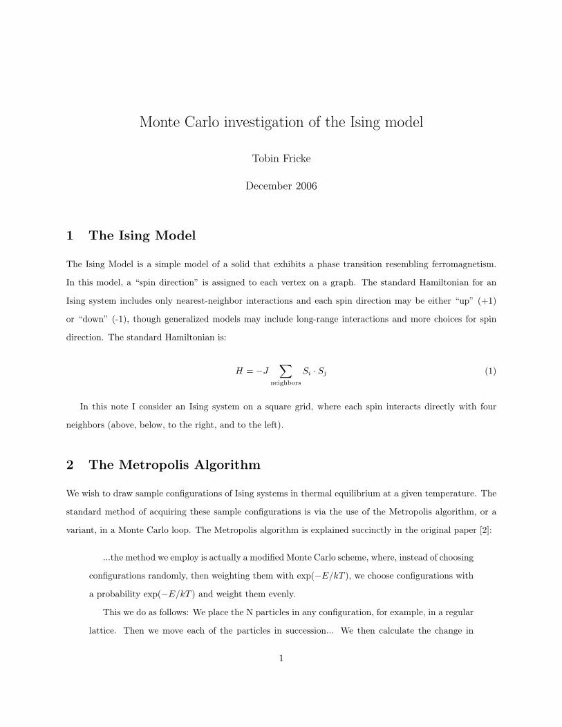
Figure 1: Magnetization per site, versus temperature.

3 Results

I implemented a Metropolis-based Monte Carlo simulation of an Ising System in Matlab and used it to

perform 5516 simulations; the code is available in the appendix. Figure 1 shows the magnetization per site

M of the final configuration in each of simulations, each with a temperature chosen randomly between 10−10

and 5. (I choose the strength of interaction as J = 1 and set Boltzmann’s constant to k = 1, so ‘temperature’

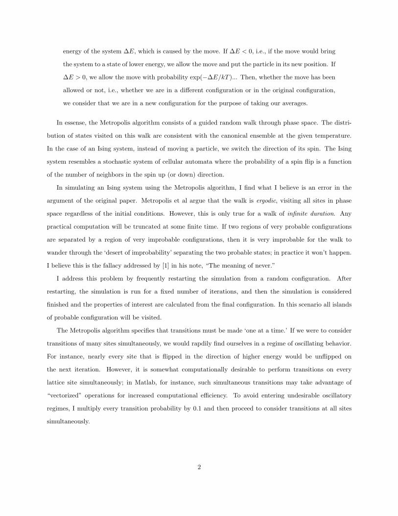
becomes dimensionless.) The energy per site is shown in Figure 2.

A phase transition is clearly visible between T = 2 and T = 2.5. At lower temperatures, the system

strongly favors the two ground states. These are the states with all spins aligned, either all up (M = 1)

or all down (M = −1). At temperatures higher than the phase transition, the spins tend to be randomly

aligned, leading to zero average magnetization (M = 0). An example Ising system in the high temperature

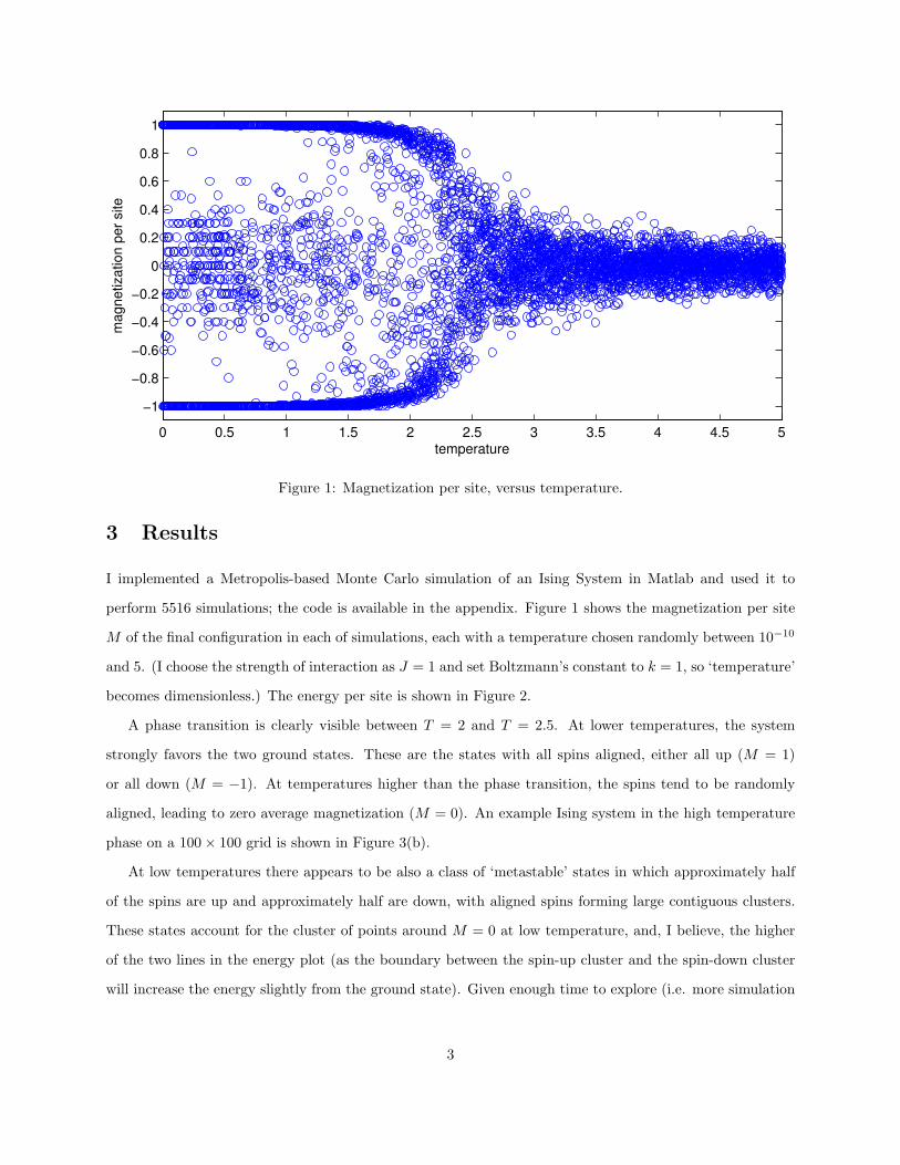
phase on a 100× 100 grid is shown in Figure 3(b).

At low temperatures there appears to be also a class of ‘metastable’ states in which approximately half

of the spins are up and approximately half are down, with aligned spins forming large contiguous clusters.

These states account for the cluster of points around M = 0 at low temperature, and, I believe, the higher

of the two lines in the energy plot (as the boundary between the spin-up cluster and the spin-down cluster

will increase the energy slightly from the ground state). Given enough time to explore (i.e. more simulation

3

0 0.5 1 1.5 2 2.5 3 3.5 4 4.5 5−4

−3.5

−3

−2.5

−2

−1.5

−1

−0.5

0en

ergy

per

site

temperature

Figure 2: Energy per site, versus temperature.

T = 1.00, M = −0.04, E = −3.61

(a) Example metastable state at T = 1

T = 5.00, M = 0.03, E = −0.81

(b) Example high-temperature phase at T = 3

Figure 3: Example states of an Ising system on a 100× 100 grid. Black square represent spin-up and whitesquare represent spin-down. The low-temperature ground states are not shown, since they consist of the gridentirely spin-up or entirely spin-down.

4

−4 −3.5 −3 −2.5 −2 −1.5 −1 −0.5 0−1

−0.8

−0.6

−0.4

−0.2

0

0.2

0.4

0.6

0.8

1

Energy per site

Mag

netiz

atio

n pe

r site

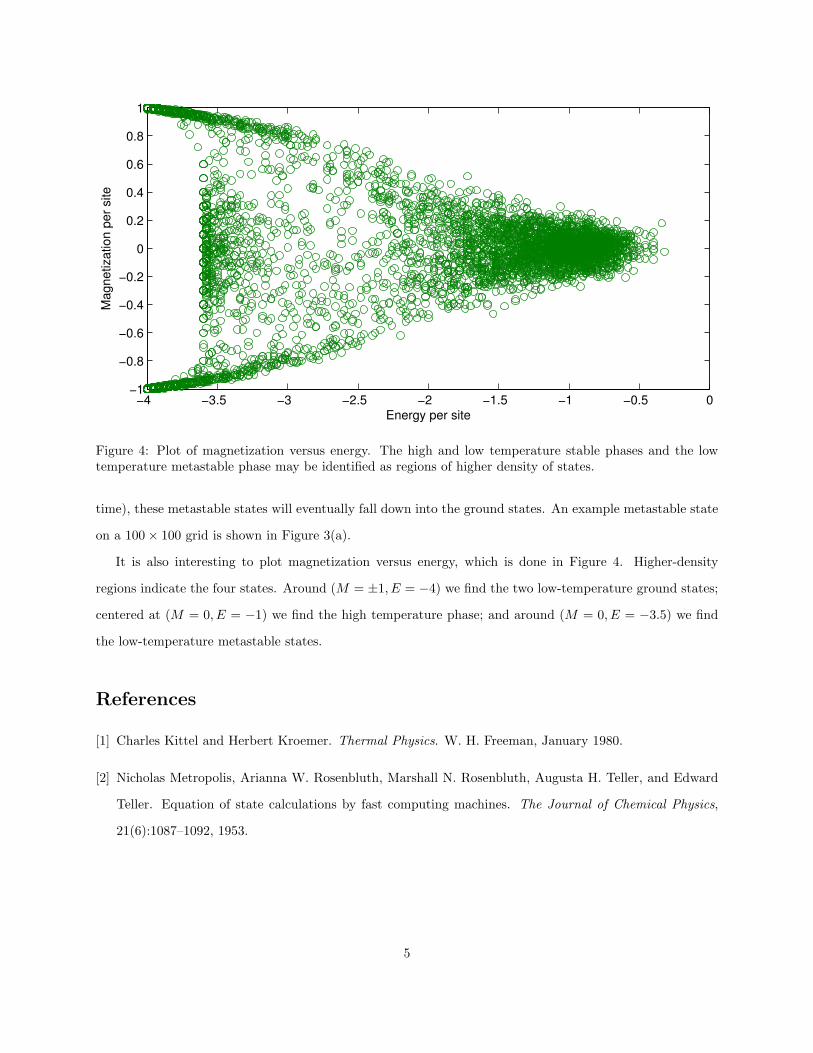
Figure 4: Plot of magnetization versus energy. The high and low temperature stable phases and the lowtemperature metastable phase may be identified as regions of higher density of states.

time), these metastable states will eventually fall down into the ground states. An example metastable state

on a 100× 100 grid is shown in Figure 3(a).

It is also interesting to plot magnetization versus energy, which is done in Figure 4. Higher-density

regions indicate the four states. Around (M = ±1, E = −4) we find the two low-temperature ground states;

centered at (M = 0, E = −1) we find the high temperature phase; and around (M = 0, E = −3.5) we find

the low-temperature metastable states.

References

[1] Charles Kittel and Herbert Kroemer. Thermal Physics. W. H. Freeman, January 1980.

[2] Nicholas Metropolis, Arianna W. Rosenbluth, Marshall N. Rosenbluth, Augusta H. Teller, and Edward

Teller. Equation of state calculations by fast computing machines. The Journal of Chemical Physics,

21(6):1087–1092, 1953.

5

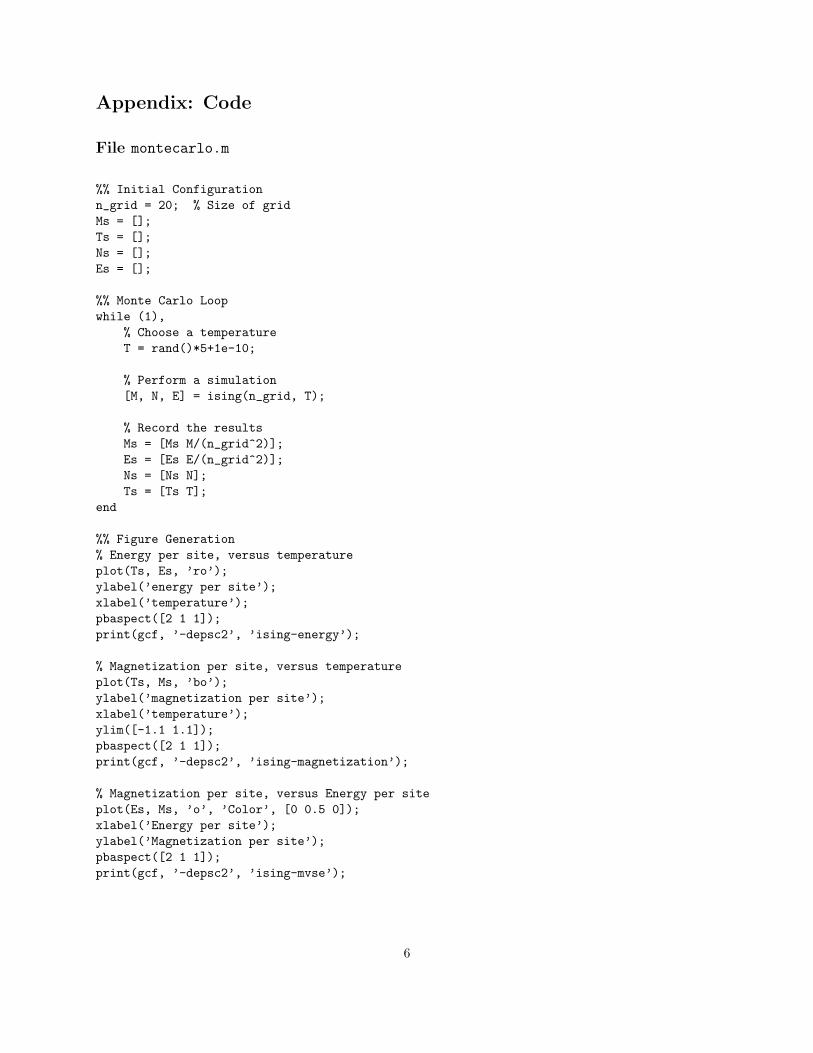
Appendix: Code

File montecarlo.m

%% Initial Configurationn_grid = 20; % Size of gridMs = [];Ts = [];Ns = [];Es = [];

%% Monte Carlo Loopwhile (1),

% Choose a temperatureT = rand()*5+1e-10;

% Perform a simulation[M, N, E] = ising(n_grid, T);

% Record the resultsMs = [Ms M/(n_grid^2)];Es = [Es E/(n_grid^2)];Ns = [Ns N];Ts = [Ts T];

end

%% Figure Generation% Energy per site, versus temperatureplot(Ts, Es, ’ro’);ylabel(’energy per site’);xlabel(’temperature’);pbaspect([2 1 1]);print(gcf, ’-depsc2’, ’ising-energy’);

% Magnetization per site, versus temperatureplot(Ts, Ms, ’bo’);ylabel(’magnetization per site’);xlabel(’temperature’);ylim([-1.1 1.1]);pbaspect([2 1 1]);print(gcf, ’-depsc2’, ’ising-magnetization’);

% Magnetization per site, versus Energy per siteplot(Es, Ms, ’o’, ’Color’, [0 0.5 0]);xlabel(’Energy per site’);ylabel(’Magnetization per site’);pbaspect([2 1 1]);print(gcf, ’-depsc2’, ’ising-mvse’);

6

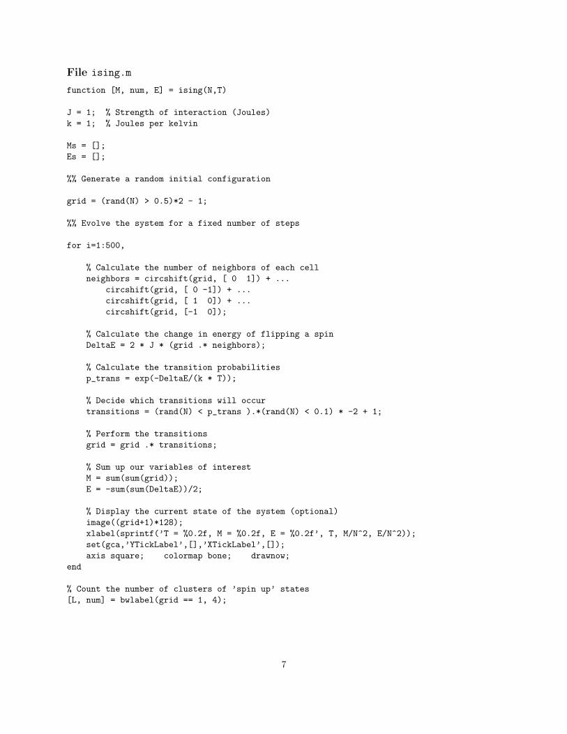
File ising.m

function [M, num, E] = ising(N,T)

J = 1; % Strength of interaction (Joules)k = 1; % Joules per kelvin

Ms = [];Es = [];

%% Generate a random initial configuration

grid = (rand(N) > 0.5)*2 - 1;

%% Evolve the system for a fixed number of steps

for i=1:500,

% Calculate the number of neighbors of each cellneighbors = circshift(grid, [ 0 1]) + ...

circshift(grid, [ 0 -1]) + ...circshift(grid, [ 1 0]) + ...circshift(grid, [-1 0]);

% Calculate the change in energy of flipping a spinDeltaE = 2 * J * (grid .* neighbors);

% Calculate the transition probabilitiesp_trans = exp(-DeltaE/(k * T));

% Decide which transitions will occurtransitions = (rand(N) < p_trans ).*(rand(N) < 0.1) * -2 + 1;

% Perform the transitionsgrid = grid .* transitions;

% Sum up our variables of interestM = sum(sum(grid));E = -sum(sum(DeltaE))/2;

% Display the current state of the system (optional)image((grid+1)*128);xlabel(sprintf(’T = %0.2f, M = %0.2f, E = %0.2f’, T, M/N^2, E/N^2));set(gca,’YTickLabel’,[],’XTickLabel’,[]);axis square; colormap bone; drawnow;

end

% Count the number of clusters of ’spin up’ states[L, num] = bwlabel(grid == 1, 4);

7