on the complexity of stratified logics - diunitovercelli/works/phdthesis-vercelli.pdf · we use to...
TRANSCRIPT

Universita degli Studi di Torino
Scuola di Dottorato in Scienze e Alta Tecnologia
Tesi di Dottorato di Ricerca in Scienze e Alta TecnologiaIndirizzo: Matematica
ON THE COMPLEXITY OFSTRATIFIED LOGICS
Luca VercelliAdvisor: prof. Luca Roversi
XXII Ciclo, 2 Febbraio 2010.

ii

Abstract
This work deals with Implicit Computational Complexity, a research area that characterizesthe Computational Complexity Classes by means of formal tools that are independent fromTuring machines, the standard model of reference for such characterizations.
Our primarymotivation is the comparison of two different traditions used to characterizethe class FPTIME of the polynomial time computable functions. On one side, FPTIMEcan be captured by Intuitionistic Light Affine Logic (ILAL), a logic derived from LinearLogic, characterized by the structural invariant Stratification. On the other side, FPTIMEcan be captured by Safe Recursion on Notation (SRN), an algebra of functions based onPredicative Recursion, a restriction of the standard recursion schema used to define primitiverecursive functions. Stratification and Predicative Recursion seem to share common underlyingprinciples, whose study is the main subject of this work.
The starting point is a known result. Under natural and straightforward assumptions,a relation between Stratification and Predicative Recursion exists. It takes the form of acompositional embedding of a fragment BC– of SRN into ILAL.
We propose two different extensions of such an embedding.The first extension follows from a systematic and uniform analysis of the deductive
systems, that we call subsystems, we obtain inside MS, a multimodal and stratified frameworkwe introduce in this work.
MS generates subsystems. Two features characterize every subsystemP of MS. (i) Everyderivation of P embodies the same Stratification principle we find in ILAL. (ii) Every P isdefined by fixing an arbitrary set of modal operators, in analogy to the two modalities ofILAL, and choosing deductive rules in a well-defined set of rules that generalize those onesin ILAL. The point of having many modalities is to extend the set of derivations-as-programsavailable in P. The framework allows a “wild” arbitrariness in the definition of subsystemsP, so it is often the case that P is polynomial time unsound, i.e. it can compute functionsoutside FPTIME. We need to develop polynomial time soundness criteria to distinguish insideMS those subsystems that only develop polynomial time sound computations.
The starting technical tool todevise criteria isContext Semantics. Once given such semanticsflavored criteria, we supply somepurely syntactic and decidable criteria, that allow todistinguishif a given subsystem P of MS is polynomial time sound or polynomial time unsound justobserving the syntactic form of the rules of P. Among the syntactic criteria there is the onethat also determines the maximal polynomial time sound subsystems of MS, which are thosesubsystems that, fixed a set of modalities, contain the largest set of derivations-as-programswe use to control how the normalization proceeds.
We have identified two subsystems of MS worth mentioning.The first subsystem is PM
LTS. It is as computationally complex as the multiplicative
fragment of Linear Logic, but it is a bit more expressive: PMLTS
contains among its proofsthose ones encoding Church Numerals and the first basic operations on them.
The second subsystem is soLAL, a multimodal generalization of ILAL. soLAL allows usto partially fulfill the initial goal of finding a relation between Stratification and PredicativeRecursion. Indeed, we can embed into soLAL a fragment SRN– of SRN such that BC– (SRN– ( SRN.

Aswe said, a secondkindof extensionof the embedding fromBC– into ILAL is considered,independent from MS.We introduce Light Affine Logic by Levels (LALL), an affine deductivesystem based on a weaker form of the Stratification principle. While soLAL uses manymodalities, LALL preserves the two modalities present in ILAL. Crucially exploiting theweaker form of Stratification of LALL, and the possibility of freely introducing recursivetypes without altering the complexity cost of the normalization of LALL, we show that all thefinite fragments of SRN programs compositionally embed into LALL.
Summing up, we investigate how to make the relation between Stratification and Pred-icative Recursion closer. We base our work on two, somewhat orthogonal, approaches. Onone side, we generalize the modal aspects of ILAL, while preserving its original notion ofStratification. On the other, we exploit a generalization of the Stratification, while preservingthe original set of modal operators. Both the lines of investigation this work develops movethe relation between Predicative Recursion and Stratification a step forward. Despite of this,none of them is able to capture the whole SRN, at least not in the standard way.
What we believe we learn thanks to this work is that the very abstract principles FPTIMErelies on are still hidden in the syntactic bureaucracy that still contaminates systems likeSRN, ILAL, soLAL, and LALL.
ii

Ringraziamenti
Ringrazio in particolar modo il mio relatore, prof. Luca Roversi, che ha dedicato davveromolto tempo a seguire me e il mio lavoro.
Ringrazio tutto il gruppo “Formal Methods in Computing”, ex gruppo λ, che e stato perme un ambiente molto accogliente.
Ringrazio il Dipartimento di Matematica, che mi ha permesso di lavorare insieme alDipartimento di Informatica, permettendomi cosı di sviluppare argomenti che — a mioavviso — interessano entrambi i Dipartimenti.
Tra le tante persone con le quali ho lavorato, un grazie particolare va a Ugo Dal Lago, perle utili discussioni che hanno dato origine ai primi risultati presenti in questa tesi.
Grazie infine a tutte le persone che mi sono state vicine durante la stesura della tesi, unperiodo che ricordo come decisamente stressante: Daniela, mia madre, mio fratello, e anchemio padre, il quale sono sicuro mi e stato vicino, pur essendo mancato da ormai 5 anni.
Acknowledgements
Really many thanks to my advisor, prof. Luca Roversi, who dedicated so much time tofollow me up and to supervise this work.
Thanks to the whole “Formal Methods in Computing” group, ex λ-group, that providedan hospitable working environment to me.
Thanks to the Department of Mathematics, that allowed me to work together with theDepartment of Computer Science, developing subjects that — at least in my opinion —mayinterest both the Departments.
In order to write my thesis, I have chatted with several people. Thanks in particular toUgo Dal Lago for the useful discussions that lead to the first results presented in this work.
At last, thanks to all the people that have been close to me during the stressing period ofthe writing: Daniela, my mother, my brother, and my father too, who passed away 5 yearsago.
iii

iv

Contents
Abstract i
Acknowledgements iii
Contents v
1 Introduction 1
1.1 State of the art . . . . . . . . . . . . . . . . . . . . . . . . . . . . . . . . . . . . . 11.2 The problem . . . . . . . . . . . . . . . . . . . . . . . . . . . . . . . . . . . . . . 41.3 Contribution . . . . . . . . . . . . . . . . . . . . . . . . . . . . . . . . . . . . . . 51.4 Guideline for the reader. . . . . . . . . . . . . . . . . . . . . . . . . . . . . . . . 10
2 Preliminaries 11
2.1 Proofs as Programs . . . . . . . . . . . . . . . . . . . . . . . . . . . . . . . . . . 112.2 Computational Complexity . . . . . . . . . . . . . . . . . . . . . . . . . . . . . 132.3 Linear Logic, Affine Logic, and Proof nets . . . . . . . . . . . . . . . . . . . . . 142.4 Light logics, ILAL and SLL . . . . . . . . . . . . . . . . . . . . . . . . . . . . . . 172.5 Implicit Computational Complexity . . . . . . . . . . . . . . . . . . . . . . . . 182.6 Algebras of functions, and Kleene functions . . . . . . . . . . . . . . . . . . . . 182.7 Safe Recursion on Notation . . . . . . . . . . . . . . . . . . . . . . . . . . . . . 192.8 Ramified Recurrence . . . . . . . . . . . . . . . . . . . . . . . . . . . . . . . . . 192.9 Relationship between light logics and algebras of functions . . . . . . . . . . . 212.10 Relations, Orders, Preorders. . . . . . . . . . . . . . . . . . . . . . . . . . . . . 222.11 Set-theoretical notations . . . . . . . . . . . . . . . . . . . . . . . . . . . . . . . 22
3 The framework MS 25
3.1 Meta-Proof nets and Proof nets . . . . . . . . . . . . . . . . . . . . . . . . . . . 253.2 Subsystems . . . . . . . . . . . . . . . . . . . . . . . . . . . . . . . . . . . . . . . 333.3 Normalization . . . . . . . . . . . . . . . . . . . . . . . . . . . . . . . . . . . . . 343.4 Technical considerations . . . . . . . . . . . . . . . . . . . . . . . . . . . . . . . 40
3.4.1 Abstract Rewriting Systems . . . . . . . . . . . . . . . . . . . . . . . . . 403.4.2 The definition of Size . . . . . . . . . . . . . . . . . . . . . . . . . . . . . 413.4.3 Why SLL is not a subsystem of MS . . . . . . . . . . . . . . . . . . . . . 44
4 Polynomiality in MS 47
4.1 Polynomial time and size . . . . . . . . . . . . . . . . . . . . . . . . . . . . . . 484.2 Following ILAL . . . . . . . . . . . . . . . . . . . . . . . . . . . . . . . . . . . . 50
v

4.3 Semantical Criteria for Polytime Soundness . . . . . . . . . . . . . . . . . . . . 524.3.1 Context semantics: definitions . . . . . . . . . . . . . . . . . . . . . . . 524.3.2 Properties of the Context semantics . . . . . . . . . . . . . . . . . . . . 564.3.3 Strong Polytime and Spindles . . . . . . . . . . . . . . . . . . . . . . . . 594.3.4 A first Criterion for Polynomial Time Soundness. . . . . . . . . . . . . 644.3.5 Strong Determinacy . . . . . . . . . . . . . . . . . . . . . . . . . . . . . 67
4.4 Syntactical Criteria for Polytime Soundness . . . . . . . . . . . . . . . . . . . . 674.4.1 Augmented subsystems . . . . . . . . . . . . . . . . . . . . . . . . . . . 674.4.2 Relations among Modalities . . . . . . . . . . . . . . . . . . . . . . . . . 704.4.3 Maximality in MS . . . . . . . . . . . . . . . . . . . . . . . . . . . . . . . 73
4.5 Infinite modalities . . . . . . . . . . . . . . . . . . . . . . . . . . . . . . . . . . . 81
5 Computational Properties in MS 83
5.1 About Cut-elimination . . . . . . . . . . . . . . . . . . . . . . . . . . . . . . . . 835.2 About Confluence . . . . . . . . . . . . . . . . . . . . . . . . . . . . . . . . . . . 84
6 Interesting Subsystems of MS 89
6.1 Quasi-linear Space . . . . . . . . . . . . . . . . . . . . . . . . . . . . . . . . . . 906.2 soLAL . . . . . . . . . . . . . . . . . . . . . . . . . . . . . . . . . . . . . . . . . . 976.3 Conclusions about soLAL and SRN . . . . . . . . . . . . . . . . . . . . . . . . . 102
7 An alternative approach: LALL 105
7.1 Light Affine Logic by Levels . . . . . . . . . . . . . . . . . . . . . . . . . . . . . 1067.2 LALL is polytime . . . . . . . . . . . . . . . . . . . . . . . . . . . . . . . . . . . 1087.3 Preliminary notions about SRN . . . . . . . . . . . . . . . . . . . . . . . . . . . 1097.4 Preliminary useful proof nets in LALL . . . . . . . . . . . . . . . . . . . . . . . 1097.5 Embedding SRN into LALL . . . . . . . . . . . . . . . . . . . . . . . . . . . . . 114
8 Further directions 119
8.1 Beyond soLAL . . . . . . . . . . . . . . . . . . . . . . . . . . . . . . . . . . . . . 1198.1.1 co-soLAL . . . . . . . . . . . . . . . . . . . . . . . . . . . . . . . . . . . . 1208.1.2 soLAL∞ . . . . . . . . . . . . . . . . . . . . . . . . . . . . . . . . . . . . 1228.1.3 IEAL . . . . . . . . . . . . . . . . . . . . . . . . . . . . . . . . . . . . . . 123
8.2 Generalizations . . . . . . . . . . . . . . . . . . . . . . . . . . . . . . . . . . . . 1248.2.1 Generalized Contractions . . . . . . . . . . . . . . . . . . . . . . . . . . 1248.2.2 Levels . . . . . . . . . . . . . . . . . . . . . . . . . . . . . . . . . . . . . 1258.2.3 Untyped Proof nets, Recursive Types . . . . . . . . . . . . . . . . . . . 132
A Encoding from SRN= to soLAL 135
A.1 The details on the map from SRN= to soLAL . . . . . . . . . . . . . . . . . . . 135A.1.1 Basic datatypes . . . . . . . . . . . . . . . . . . . . . . . . . . . . . . . . 135A.1.2 Basic proof nets . . . . . . . . . . . . . . . . . . . . . . . . . . . . . . . . 136A.1.3 Configurations and transition function between them . . . . . . . . . . 137A.1.4 The iteration . . . . . . . . . . . . . . . . . . . . . . . . . . . . . . . . . . 139
Index 159
Table of Symbols 160
vi

Bibliography 162
vii

viii

Chapter 1
Introduction
1.1 State of the art
Implicit Computational Complexity. Our work relates with Implicit Computational Com-plexity, in the following ICC. We will briefly recall what it is. The theory of ComputationalComplexity, or CC [Pap94], classifies the computable functions in computational classes: forexample, FPTIME is the class of all the functions computable with a Turing machine in a time thatis polynomial in the size of the input, and FPSPACE is the class of all the functions computablewith a Turing machine using an amount of memory that is polynomial in the size of the input. Now,though the computational model of Turing machines has been a standard for years, it isquite heavy. We mean, for example, it is very difficult to write any equation describing acomplexity class, and this is because the model of Turing machines is not suitable for that.The ICC tries to characterize the same complexity classes in a way independent from sucha model. For this purpose, several different approaches are used. We will deal in particularwith two approaches: algebras of functions and light logics.
In the first approach, a computational class (say, FPTIME) can be described as an algebra offunctions, i.e. a set of functions containing some basic functions and closed under some oper-ators over functions. This is a style common in recursion theory, where e.g. the computablefunctions can be represented as the algebra of functions described by Kleene [Kle36, Odi89].In Sections 2.7 and ff. we will recall two important systems of this kind, SRN [BC92] and theRamified Recurrence [Lei93], that both characterize the class FPTIME.
On the other side, light logics provide a completely different approach to ICC. The so-called Curry-Howard correspondence [How80, SrU06] identifies an analogy between proofs andprograms. More precisely, there exists a bijection between proofs of intuitionistic and purelyimplicative logic, in the formalism of natural deduction, and programs, in the formalism oftyped λ-calculus. The execution of programs corresponds to the normalization of proofs. So,a class of programs also corresponds to a class of proofs. This is the idea underlying light logics:a computational class can be represented using a logic. Such a logic must be even weakerthan the intuitionistic logic, hence the name light. Some computational classes have alreadybeen characterized that way. Examples of light logics are LLL [Gir98], ILAL [AR02] and SLL[Laf04], all characterizing FPTIME; ELL, characterizing the class of elementary functions[DJ03]; STAB, characterizing FPSPACE [GMR08]. Most of them are logics derived from theLinear Logic, or LL [Gir87]. Some more details will be found in Chapter 2.
In this work, we will never refer directly to λ-calculus, nor to the Curry-Howard corre-
1
CHAPTER 1. INTRODUCTION
A ⊢ Aidentity
Γ ⊢ A ∆,A ⊢ BΓ,∆ ⊢ B
cut
Γ ⊢ AΓ,B ⊢ A
W⊢ A
h
Γ,A ⊢ BΓ ⊢ A⊸ B
⊸RΓ ⊢ A ∆,B ⊢ CΓ,∆,A⊸ B ⊢ C
⊸L
Γ ⊢ A ∆ ⊢ BΓ,∆ ⊢ A ⊗ B
⊗RΓ,A,B ⊢ CΓ,A ⊗ B ⊢ C
⊗L
Γ ⊢ AΓ ⊢ ∀α.A
∀R (∗)Γ,A[B/α]⊢ B
Γ,∀α.A ⊢ B∀L
A ⊢ B!A ⊢ !B
!⊢ B⊢ !B
!!A, !A, Γ ⊢ B!A, Γ ⊢ B
contraction
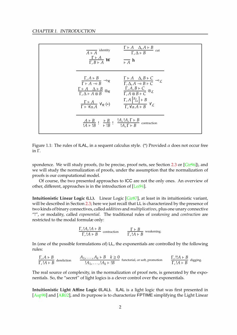
Figure 1.1: The rules of ILAL, in a sequent calculus style. (*) Provided α does not occur freein Γ.
spondence. We will study proofs, (to be precise, proof nets, see Section 2.3 or [Gir96]), andwe will study the normalization of proofs, under the assumption that the normalization ofproofs is our computational model.
Of course, the two presented approaches to ICC are not the only ones. An overview ofother, different, approaches is in the introduction of [Lei94].
Intuitionistic Linear Logic (LL). Linear Logic [Gir87], at least in its intuitionistic variant,will be described in Section 2.3; here we just recall that LL is characterized by the presence oftwokinds of binary connectives, called additives andmultiplicatives, plus one unary connective“!”, or modality, called exponential. The traditional rules of weakening and contraction arerestricted to the modal formulæ only:
Γ, !A, !A ⊢ BΓ, !A ⊢ B
contractionΓ ⊢ BΓ, !A ⊢ B
weakening.
In (one of the possible formulations of) LL, the exponentials are controlled by the followingrules:
Γ,A ⊢ BΓ, !A ⊢ B
derelictionA1, . . . ,Ak ⊢ B k ≥ 0
!A1, . . . , !Ak ⊢ !Bfunctorial, or soft, promotion
Γ, !!A ⊢ BΓ, !A ⊢ B
digging.
The real source of complexity, in the normalization of proof nets, is generated by the expo-nentials. So, the “secret” of light logics is a clever control over the exponentials.
Intuitionistic Light Affine Logic (ILAL). ILAL is a light logic that was first presented in[Asp98] and [AR02], and its purpose is to characterize FPTIME simplifying the Light Linear
2

1.1. STATE OF THE ART
Logic of [Gir98]. The complete list of the rules of ILAL is in Figure 1.1, in a sequent calculusstyle. We now try to explain how these rules are obtained. They are derived from the rulesof LL. In order to lower the complexity of the reductions, w.r.t. LL, ILAL forbids the derelictionand digging rules, and allows the functorial promotion with at most one premise:
A1, . . . ,Ak ⊢ B k ∈ 0, 1!A1, . . . , !Ak ⊢ !B
!.
At this point, the logic that we have got is too weak. Indeed every reduction is performedin polynomial time, but it is not obvious (maybe it is impossible?) to represent the Churchnumerals inside it, and they are usually required to represent some form of iteration. Thesolution involves two steps: (i) the introduction of another modality “§” (paragraph), that allowsa promotion rule more liberal than the “!”, but which does not admit contraction, and (ii) theintroduction of the free weakening (W) rule. W is the real difference between ILAL and LLL.The dynamic of the reduction of the free weakening rules allows to erase pieces of proofs ina simple way, without any need for additives. As observed in [Asp98]: “the abstinence fromweakening leads to inessential syntactical complications“. So, ILAL just has multiplicative andexponential connectives.
The free weakening has also some negative consequences, that force ILAL to be (i) intu-itionistic, and (ii) to include the somewhat weird rule h of Figure 1.1. The interested readeris referred to Section 2.4.
Algebras of Functions vs Light Logics. Both ILAL and SRN, we already said, are able tocharacterize the functions in FPTIME. It is reasonable, thus, to compare these two systems.
Both ILAL and SRN allow the representation of all the polytime Turing machines [AR02,Cob65, BC92]. However, at first sight, programming in ILAL seems easier than in SRN. Thereason is that ILAL handles higher-order types, while SRN only handles first-order functions,from natural numbers to natural numbers. So, for example, [Cas97, Hof03] show that thereexist simple algorithms that cannot be written – at least not easily – in the systems basedon predicative recurrence. Some of these algorithms can be written in ILAL, instead (but ofcourse not all: the nesting of iteration is limited in ILAL, as well).
On the other side, two facts suggest that SRN could express in a simple way programsthat ILAL cannot. First, ILAL is strongly polytime, that is polytime under every strategy ofreduction [Ter07], while SRN is weakly but not strongly polytime, i.e. it is polytime onlyunder some precise strategy [BW96, BDLM06]. And it is reasonable that many more weaklypolytime algorithms exist, than strongly polytime. Second, at the moment it is not known atranslation that compositionally translates programs of SRN into proofs of ILAL. In [MO04],it is shown a simple encoding that translates the programs of BC–, a proper subset of theprograms of SRN, into ILAL, and it is also shown that it is not possible to extend the sameencoding to the whole SRN (more details in Section 2.9). By the way, at the moment it is notknown if BC– captures all FPTIME, or not. In the samework [MO04] it is also shown that it ispossible to extendBC– to some BC± that captures FPTIME and that compositionally embedsinto ILAL; however, BC± does not help understanding the intrinsic differences between SRNand ILAL, since it contains primitives extraneous to SRN. The situation is summed up inFigure 1.2: it seems necessary to extend ILAL to some system (3) that can contain SRN. Or,at least, we would like to find some extension (2) that captures at least some strict extension(1) of BC–.
3

CHAPTER 1. INTRODUCTION
PTIMETuring Machines SRN ? (3)
? (1) ? (2)
BC± BC– ILAL
⊇ ⊇
⊇
⊇ ⊇
Figure 1.2: Relations between SRN and ILAL.
1.2 The problem
Extending ILAL. The origin that justifies this work is the search for some extension ofILAL, that nevertheless characterizes the class FPTIME. It should be clear that many differentextensions are possible, as we can imagine a large variety of rules to add to ILAL; the problemis not to escape from the domain of polynomial time. As an example of how extending ILALmay increase its expressiveness, we will consider two different extensions of ILAL by meansof some forms of dereliction. Let us consider ILAL! as ILAL plus the dereliction rule (alreadypresentedabove). ILAL! is notpolytime, since it allows towrite an hyper-exponential functionthat we are going to describe. Let us consider the following type for Church numerals:
N = ∀α.!(α⊸ α)⊸ α⊸ α (the same as in LL).
Then, one can build the following proof nets (i.e. proofs), with the expected semantics:
succ : N⊸N
add : N⊸N⊸N
mul : !N⊸N⊸N
exp : !!N⊸N⊸N
hypexp : !!!N⊸N⊸N
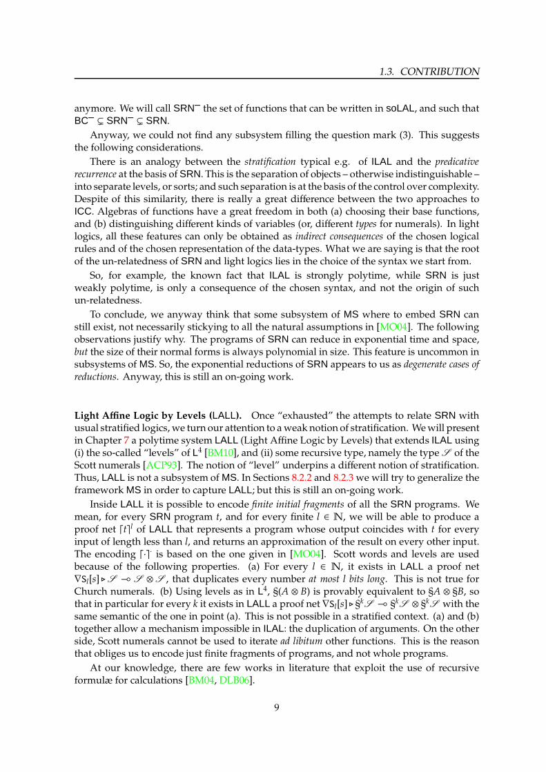
This means, for example, that it is possible to build a proof of N ⊸ N called succ that,whenever cut with a numeral n, reduces to n + 1. Addition in fact is obtained concatenatingnumerals. Each one of the last three functions is obtained iterating the one that precedes it.For example, multiplication is in Figure 1.3a.
So, ILAL! does not work for our purposes. We may then imagine to allow the derelictionon the “§” instead than on the “!”:
Γ,A ⊢ BΓ, §A ⊢ B
D§.
We obtain a system ILAL§ that does not enjoy cut elimination: there is no way to reducea §-dereliction in cut with a §-box with some !-premises. We are not frightened by thisinconvenience: the proof net containing irreducible cuts will be considered normal forms.We now show that ILAL§ is not polytime. It is possible to use the following type for theChurch numerals:
N = ∀α.!(α⊸ α)⊸ §(α⊸ α) (as in ILAL).
4

1.3. CONTRIBUTION
o
⊸R
⊸R
⊸L
⊸L 0
∀L
!
⊸L
add
!
!N⊸N⊸N
N⊸N
N
NN⊸N
!(N⊸N)
N⊸N
N⊸N⊸NN
!(N⊸N)⊸N⊸N
!N
N
(a)
o
⊸R
⊸R
⊸L
D 0
⊸L
∀L
!
⊸L
add
!
!N⊸N⊸N
N⊸N
N
N
§(N⊸N)
N⊸N
!(N⊸N)
N⊸N
N⊸N⊸NN
!(N⊸N)⊸§(N⊸N)!N
N
(b)
Figure 1.3: Multiplication proofnet in ILALplus !-dereliction (a) and in ILALplus §-dereliction(b). Notice thatN denotes a different type in the two cases.
Nowwe can write, in ILAL§, all the functions that we already encoded in ILAL!, and with thesame type. For example, multiplication is in Figure 1.3b. Thus ILAL§ is not polytime.
The previous two examples make clear that, even if a great number of extensions of ILAL arepossible, we need some way to understand which one are polytime, and which one are not. We need toconsider a large number of possible extensions, and to study them in a uniform way.
1.3 Contribution
The overall picture. This work has the following main goals.
1. We will present a class of light logics derived from ILAL that can be useful for the repre-sentation of computational classes. These logics will be called subsystems of a frameworkMS that this thesis introduces and studies.
2. We will compare the two approaches to ICC already described: light logics and algebrasof functions. This means that we will try to fill the question marks in Figure 1.2, alongtwo different routes.• The first route is to search for an extension of ILAL inside the subsystems of MS,arriving for example to soLAL, a subsystem that we can replace for the question mark(2) in Figure 1.2, for a suitable subsystem SRN– of SRN in place of (1).• The second route is to turn to a weaker form of stratification that MS, for the moment,does not contain. Such a weaker form is in the logical system LALL (Light Affine Logicby Levels) that we shall present, which, in a precise technical sense, can replace (3).
5
CHAPTER 1. INTRODUCTION
Rephrasing the incipit of [Lei94], getting to the above two goals will help providing insightsinto the abstract nature of computing FPTIME functions, while offering concepts and methods forgeneralizing computational complexity to computing over arbitrary structures and to higher typefunctions.
We now deepen a bit the description of our contribution.
Multimodal Stratified framework (MS). One of the focuses of this work is what we callMultimodal and Stratified framework for polytime computations [RV08, RV09], thatwewill presentin Chapter 3. Now we sketch the main features of MS. The framework allows to study in auniform way a variety of different light logics, all derived from LL, and all described in theformalism of proof nets. Please notice that instead, in this Introduction, we have found easierto deal with the derivation trees of sequent calculus than with the proof nets. The variouslight logics that we will consider will be called subsystems of MS.
Before any formal definition of the framework MS, we prefer to underline what are thekey points of all its subsystems. (i) Each subsystemP is defined as a particular set of buildingrules, i.e. rules that allow the inductive construction of proof nets. We will denote PN(P) theset of such proof nets. Along the work, we shall refer informally to the elements of PN(P) asthe proof nets ofP, andwe shall say thatP allows a rule RwheneverR ∈ P. (ii) All the proof netsthat we consider are intuitionistic, that is proof nets with one only conclusion. (iii) Amongthe possible rules, there is the linear kernel of LL, whose rules will be recalled in Section 2.3and 3.1. This kernel includes the rules for multiplicative connectives and for second-orderquantifiers, but not the rules for additive connectives. This fact is somewhat traditional in anaffine context: the additives can be defined using the free weakening and the second orderquantification. (iv) The exponential rules, or modal rules, derived from LL, are generalizedin order to handle an arbitrary number of modalities, and not only the one of LL or the twoones of ILAL. This is why we say the framework ismultimodal. This is analogous e.g. to whathappens in [Sch94]. From the technical point of view, multimodality is obtained allowingthe modalities to vary over a fixed – but arbitrary – set X, that usually will be finite, anddefining the framework in a way that X is used as a free parameter. (v) On the other side,however, the framework puts some restrictions on the exponential rules. Remember that weare generalizing ILAL, so exactly as in ILAL the dereliction and digging rules are forbidden.These restrictions force the proof nets to reduce in a peculiar way: the promotion rules, insidea proof net, mark off some regions (“boxes”) that reduce independently the one from theother, and the number of nested boxes around a given node of a proof net do not vary duringa reduction. This behavior is called stratification, hence the name of the framework.
And now, a slightly more formal definition of the framework. The framework is madeup of a set of meta-building rules and meta-normalization steps, that will be defined resp. inSection 3.1 and 3.3. The meta-building rules allow the construction of meta-proof nets, i.e.proof nets with some parameters that may vary over a given set of modalities X. Forexample,
Γ,mA, nA ⊢ BΓ, qA ⊢ B
Yq(m, n) m, n, q ∈ X
is a meta-building rule, that can be instantiated to the “usual” contraction provided ! ∈ Xand m = n = q =!. The meta-normalization steps map meta-proof nets into meta-proof nets.So, this implies that, once instantiated the parameters of the meta-normalization steps, weget normalization steps from proof nets to proof nets. For every fixed set X of modalities,
6

1.3. CONTRIBUTION
d ...
Y
Cut
b
Y
Y
g B
f
u
e mA
τ ρ
Figure 1.4: The structure between e and f is an example of spindle. If the spindle is dangerous,it is possible connect it to some g labelled B = mA′.
BX is the set of all the instances of the meta-building rules, with modalities varying overX. Similarly, R(BX) is the set of all the instances of the meta-normalization steps. At last, asubsystem of MS is simply a subset P ⊆ BX. Each subsystem uniquely identifies (1) a set ofproof nets PN(P), that can be built using all and only the building rules in P, and (2) a set ofnormalization steps R(P) ⊆ PN(P)2, which contains all and only the normalization steps inR(BX) that correctly map proof nets of PN(P) into proof nets of PN(P).
Polytime subsystems. Up to here, we have described the statical properties of MS. But,as we already said, every subsystem P of MS identifies in fact a class of programs, and weare interested to the behavior of such programs. As a consequence of the constraints givenby stratification, fixed a subsystem P ⊆ BX, every reduction in P is performed in at most anelementary time in the size of the proof (read also: “every program executes in an elementarytime in the size of the arguments”).
We characterize those subsystems in which the reductions are performed in polytime(i.e. polynomial time). PMS is the class containing such subsystems. We describe howin Chapter 4. There, we will define two basic notions: (a) a dangerous spindle, recalled inFigure 1.4, that is a geometrical configuration that can be present inside the proof nets ofMS, made up of two and only two paths connecting a contraction to a box; and (b) a sensiblesubsystem, that is a subsystem endowedwith a sufficient number of rules, enough to encodea minimum amount of programs. The Polynomiality Criterion (Proposition 4.3.40) tells that:
A sensible subsystem is polytime if and only if it does not allow the constructionof dangerous spindles.
The notions of spindle and dangerous spindle, as well as the proof of the PolynomialityCriterion, rely on the formal technology of context semantics, or CS, [DL08]. Notice anywaythat the spindles provide an abstraction over CS: once defined them, only a small amount ofCS is needed to understand if P can build a dangerous spindle, or not.
Anyway, this small amount of CS is still too much. We prove some more properties,more syntactical, that still discriminate among polytime and non-polytime subsystems, and
7
CHAPTER 1. INTRODUCTION
'
&
$
%
Subsystems of BX
u∅
uBX
u u u u u uu u u u u u uu u u u u u u
u u u u u u
Maximal Polynomial Systems
Polytime subsystems,ILAL included if X ⊇ !, §
Not polytime subsystems,IEAL included if X ⊇ !, §
ILAL
IEAL
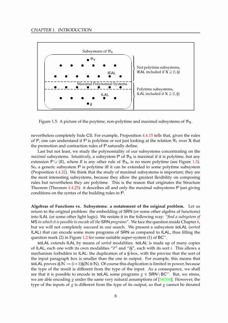
Figure 1.5: A picture of the poytime, non-polytime and maximal subsystems ofBX.
nevertheless completely hide CS. For example, Proposition 4.4.15 tells that, given the rulesof P, one can understand if P is polytime or not just looking at the relation R↑ over X thatthe promotion and contraction rules of P naturally define.
Last but not least, we study the polynomiality of our subsystems concentrating on themaximal subsystems. Intuitively, a subsystem P of BX is maximal if it is polytime, but anyextension P ∪ R, where R is any other rule of BX, is no more polytime (see Figure 1.5).So, a generic subsystem P is polytime iff it can be extended to some polytime subsystem(Proposition 4.4.32). We think that the study of maximal subsystems is important; they arethe most interesting subsystems, because they allow the greatest flexibility on composingrules but nevertheless they are polytime. This is the reason that originates the StructureTheorem (Theorem 4.4.25): it describes all and only the maximal subsystems P just givingconditions on the syntax of the building rules in P.
Algebras of Functions vs. Subsystems: a restatement of the original problem. Let usreturn to the original problem: the embedding of SRN (or some other algebra of functions)into ILAL (or some other light logic). We restate it in the following way: “find a subsystem ofMS in which it is possible to encode all theSRN programs”. We face the question inside Chapter 6,but we will not completely succeed in our search. We present a subsystem soLAL (sortedILAL) that can encode some more programs of SRN as compared to ILAL, thus filling thequestion mark (2) in Figure 1.2 for some suitable super-system (1) of BC–.
soLAL extends ILAL by means of sorted modalities: soLAL is made up of many copiesof ILAL, each one with its own modalities “i!” and “i§”, each with its sort i. This allows amechanism forbidden in ILAL: the duplication of a §-box, with the proviso that the sort ofthe input paragraph box is smaller than the one in output. For example, this means thatsoLAL proves i§N⊸ (i+1)§(N⊗N). Of course this duplication is limited in power, becausethe type of the result is different from the type of the input. As a consequence, we shallsee that it is possible to encode in soLAL some programs g ∈ SRN \BC–. But, we stress,we are able encoding g under the same very natural assumptions of [MO04]. However, thetype of the inputs of g is different from the type of its output, so that g cannot be iterated
8
1.3. CONTRIBUTION
anymore. We will call SRN– the set of functions that can be written in soLAL, and such thatBC– ( SRN– ( SRN.
Anyway, we could not find any subsystem filling the question mark (3). This suggeststhe following considerations.
There is an analogy between the stratification typical e.g. of ILAL and the predicativerecurrence at the basis of SRN. This is the separation of objects – otherwise indistinguishable –into separate levels, or sorts; and such separation is at the basis of the control over complexity.Despite of this similarity, there is really a great difference between the two approaches toICC. Algebras of functions have a great freedom in both (a) choosing their base functions,and (b) distinguishing different kinds of variables (or, different types for numerals). In lightlogics, all these features can only be obtained as indirect consequences of the chosen logicalrules and of the chosen representation of the data-types. What we are saying is that the rootof the un-relatedness of SRN and light logics lies in the choice of the syntax we start from.
So, for example, the known fact that ILAL is strongly polytime, while SRN is justweakly polytime, is only a consequence of the chosen syntax, and not the origin of suchun-relatedness.
To conclude, we anyway think that some subsystem of MS where to embed SRN canstill exist, not necessarily stickying to all the natural assumptions in [MO04]. The followingobservations justify why. The programs of SRN can reduce in exponential time and space,but the size of their normal forms is always polynomial in size. This feature is uncommon insubsystems of MS. So, the exponential reductions of SRN appears to us as degenerate cases ofreductions. Anyway, this is still an on-going work.
Light Affine Logic by Levels (LALL). Once “exhausted” the attempts to relate SRN withusual stratified logics, we turn our attention to aweak notion of stratification. Wewill presentin Chapter 7 a polytime system LALL (Light Affine Logic by Levels) that extends ILAL using(i) the so-called “levels” of L4 [BM10], and (ii) some recursive type, namely the type S of theScott numerals [ACP93]. The notion of “level” underpins a different notion of stratification.Thus, LALL is not a subsystem of MS. In Sections 8.2.2 and 8.2.3 we will try to generalize theframework MS in order to capture LALL; but this is still an on-going work.
Inside LALL it is possible to encode finite initial fragments of all the SRN programs. Wemean, for every SRN program t, and for every finite l ∈ N, we will be able to produce aproof net ⌈t⌉l of LALL that represents a program whose output coincides with t for everyinput of length less than l, and returns an approximation of the result on every other input.The encoding ⌈·⌉· is based on the one given in [MO04]. Scott words and levels are usedbecause of the following properties. (a) For every l ∈ N, it exists in LALL a proof net∇Sl[s] ⊲S ⊸ S ⊗S , that duplicates every number at most l bits long. This is not true forChurch numerals. (b) Using levels as in L4, §(A ⊗ B) is provably equivalent to §A ⊗ §B, sothat in particular for every k it exists in LALL a proof net ∇Sl[s] ⊲ §
kS ⊸ §kS ⊗ §kS with thesame semantic of the one in point (a). This is not possible in a stratified context. (a) and (b)together allow a mechanism impossible in ILAL: the duplication of arguments. On the otherside, Scott numerals cannot be used to iterate ad libitum other functions. This is the reasonthat obliges us to encode just finite fragments of programs, and not whole programs.
At our knowledge, there are few works in literature that exploit the use of recursiveformulæ for calculations [BM04, DLB06].
9

CHAPTER 1. INTRODUCTION
1.4 Guideline for the reader.
Chapter 2 contains basics knowledge about λ-calculus, proof theory, computational com-plexity, light logics and predicative recurrence. Most of the Chapter is mainly intended fornon-specialists. Section 2.7, on the other side, presents SRN, that will be required later, inChapters 6 and 7; so probably every reader wants to refer to this Section. The frameworkMS will be studied from Chapter 3 up to Chapter 6. They are quite technical; we suggestthe reader, for a first lecture, to read only the main definitions and theorems. The mostimportant are the Polynomiality Criterion (Proposition 4.3.40) and the Structure Theorem(Theorem 4.4.25); some more propositions are summed up in Figure 4.1. Chapter 7, at last,presents LALL, a light logic that is not a subsystem of MS, but that can be used to encodefinite fragments of SRN programs.
10

Chapter 2
Preliminaries
In this Sectionwe recall the basics concepts needed toput this thesis in his correct background.The Section is mainly intended for non-specialists, who need a picture of the back-
ground around this Thesis. So, it should not be surprising that most of details will be
skipped, or presented in an informal or naıve way.
A more detailed picture is e.g. in [Maz02, Sch08].
2.1 Proofs as Programs
In this Thesiswe shall dealwith proofs, in some precise formalism to be defined. However, wewill see the proofs as they were programs: we will say that our proofs normalize, thinking thatthe corresponding program executes; andwewill call results of the computation the proofs thatcannot be normalized anymore. Theorem2.1.2 shall makemore precise this correspondence:there exists a bijection betweenproofs – in the formalism of natural deduction – and programs– in the formalism of λ-calculus. We are now going to recall what are λ-calculus and naturaldeduction, in order to formalize Theorem 2.1.2.
Untyped λ-calculus. λ-calculus is a model of computation, whose programs are calledλ-terms [Bar84]. λ-terms are syntactical objects defined by the following grammar:
t, u : := x | λx.t | tu ∀x ∈ V
whereV is a countable set of symbols called variables. Every λ-term can be seen as a program;the execution of that program is given by the rule of β-reduction:
(λx.t)u→β u[t/x].
It’s possible to prove that every Turing machine can be codified into a λ-term, and of coursethere exists a Turing machine that performs the reduction of any given λ-term. So, this is amodel of calculus equivalent to Turing machines.
It is very interesting to study the semantics of these objects [AC98]. Intuitively, λ-termsare (computable) functions. But of course they cannot be functions according to the usualset-theoretical conventions, as they violate the Axiom of Foundation: tt is a correct λ-term,while no function can be applied to itself.
Anyway, this is not the matter of our work.
11

CHAPTER 2. PRELIMINARIES
In order to simplify the semantics of λ-terms, it is often convenient to consider only atyped version of the λ-calculus. This can be done in two different ways.
Typed λ-calculus: approach a la Church. Types and typed λ-terms are syntactical objectsdefined as follows:
A,B : :=α | A→ B ∀α ∈ T
t, u : := xA |(λxA.tB
)A→B|(tA→BuA
)B∀xA ∈ V
where T is a countable set of symbols called atomic types andV is as before. Typed λ-termscan be seen as a small subset of the λ-terms, just forgetting the types. Their semantics isclear: a type A is a set, and a term tA→B is a (computable) function from A to B.
Typed λ-calculus: approach a la Curry. It is defined a notion of typeability over untypedλ-terms. So, for example, λx.x is typeable because it can be endowed with a type A→ A. Itstype it is not unique, because also B→ B does the job. Only typeable λ-terms are accepted.
Expressiveness of Typed λ-calculus. In the typed settings, only a small set of Turing-computable functions can be represented. In order to restore the completeness, one possiblesolution is the introduction of some kind of fix point operator; but at the moment this is notneeded in our work. A different way to restore expressiveness (without however reachingfull Turing completeness) is the introduction of the second order quantifier, as in Girard’ssystem F [GTL89].
Proof theory. There exist some different formalisms for proofs. Each formalism tries tocapture what are the elements to make a proof correct. So, each formalism defines oneor more axiom to start with, and one or more deduction rules that are allowed to derivetheorems.
Hilbert systems use only 1 logical rule (modus ponens) and an infinite number of differentkinds of axioms. Very often, all tautologies are included among these axioms. This kind ofsystems is quite unnatural and, at the moment, they are not used when studying ICC.
Innaturaldeduction [Pra65] there are no axioms at all (well, they are hidden in the syntax),and a lot of rules. Typically this is the formalization of the approach that a mathematicianuses to find out a proof. Among these rules there are both introduction and elimination rules.One usually denotes NJ and NK resp. the intuitionistic and classical version of naturaldeduction.
In the third formalization, Gentzen’s logistic calculi or sequents calculus [Gen35], thereis exactly 1 kind of axiom (identity), 1 elimination rule (cut, quite similar tomodus ponens) anda lot of introduction rules. Gentzen denotes LJ and LK resp. the intuitionistic and classicalversion of logistic calculi. So, most of the axioms of the Hilbert systems are here turned intological rules.
The fourth – and last – formalization thatwe consider is very different: aproof net [Gir96]is a proof represented by a particular graph. Proof nets take their origin in Linear Logic,but can be applied in fact also to classical and intuitionistic logic [Rob03]. The main idea isthat in both natural deduction and logistic calculi many proofs of a same statement differjust for the – irrelevant – order of application of the logical rules; using a graph-theoretical
12

2.2. COMPUTATIONAL COMPLEXITY
representation these differences disappear, and all these proofs are identified in a single proofnet.
Cut-elimination. The first important result in proof theory is the Haupsatz:
T 2.1.1 (H (G, 1935))In both LK and LJ, the cut rule is not necessary. There exists an algorithm (called cut-elimination) that transforms every LJ (resp. LK) proof without non-logical axioms into a cut-free LJ (resp. LK) proof. In LJ this algorithm is deterministic.
This means that, if we were just interested in the set of provable sequents, the cut rulecould be avoided, and logistic calculus would be a system with only introduction rules. In acomputational perspective, on the contrary, the cut rule will have a very important role.
The algorithm of cut-elimination has also an equivalent version in NJ and NK, that wewill call normalization. Essentially, the normalization removes useless pair of introduc-tion/elimination rules.
Curry-Howard correspondence. At last, the already announced Theorem:
T 2.1.2 (C-H C)There exists a bijection between proofs of purely implicative NJ and typed λ-terms. Underthis bijection, the normalization of proofs corresponds to β-reduction of λ-terms.
The Curry-Howard correspondence suggests a model of computation based on proofsinstead than programs.
In our work we use little natural deduction, and more logistic calculi and proof nets.Every proof net stands for several NJ proofs, and every NJ proof corresponds to several LJproofs. So we can speak about Curry-Howard correspondence also between typed λ-termsand purely implicative proof nets, an between typed λ-terms and purely implicative LJproofs.
The following syntax is used for making the correspondence of Theorem 2.1.2 effective:
x : A ⊢ x : Aax
Γ, x : A ⊢ t : BΓ ⊢ λx.t : A→ B
⊸ IΓ ⊢ t : A Γ ⊢ s : A→ B
Γ ⊢ st : B⊸ E
(2.1)
Types are omitted, as they are trivially induced by the formulæ. Thanks to deductions (2.1),every proof of ⊢ A is associated to a program t such that ⊢ t : A; t is called realizer of the proof,and in some sense t is the program that provesA. Now it’s clear why the logic is intuitionisticand not classic: Amust be proved constructively. This vision is called Heyting semantics of theproofs; the interested reader can refer to [GTL89].
2.2 Computational Complexity
The objects studiedbyComputational Complexity [Pap94] are both computationally solvableproblems, and algorithms that solve them. Informally speaking, CC target is to give eachalgorithm and each problem a complexity measure; for example, how much time a solving
13

CHAPTER 2. PRELIMINARIES
program takes to execute, or how many resources does it use? So, the main aim of CC is theidentification of a hierarchy of complexity classes of problems.
In particular the theory identifies:
• a hierarchy of time classes: PTIME and EXPTIME are the classes of problems that canbe solved with a Turing Machine in resp. polynomial and exponential time in the sizeof the input.
• a hierarchy of space (that is, used memory) classes: L, PSPACE and EXPSPACE arethe classes of problems that can be solved with a Turing Machine in resp. logarithmic,polynomial and exponential space in the size of the input.
• for each one of the previous classes, a non-deterministic class: that is, the class of prob-lems that can be solved according to that complexity bound using a non-deterministicTuring Machine, which is able to make always the better choice.
• a hierarchy of computable functions: e.g. if PTIME identifies the problems solvable inpolynomial time,FPTIME identifies the class of the functions computable in polynomialtime.
There are hundreds of results actually known about CC. We just remember that:
L = NL ⊆ PTIME ⊆ NPTIME ⊆ PSPACE = NPSPACE ⊆
⊆ EXPTIME ⊆ NEXPTIME ⊆ EXPSPACE
and
PTIME ( EXPTIME L ( PSPACE ( EXPSPACE
but all the other inequalities are not known yet to be proper or not. PTIME?= NPTIME is one
of the most well-known open problems.
All ourwork concentrates on the classFPTIMEof the functions computable in polynomialtime.
2.3 Linear Logic, Affine Logic, and Proof nets
Linear Logic. The logic that we use in this work is the Linear Logic (LL) [Gir87], mainly inits intuitionistic and affine form [AR02].
Here we sum up the main features of the LL, without any hope to be exhaustive.
• The sequent calculi systems LJ and LK are made up of both logical and structural rules.Traditionally, structural rules (contraction and weakening) are accepted by every logician,and the studies concentrate on the logical rules.• On the contrary LL focuses on the structural rules.• LL is built around a kernel of rules MALL (Multiplicative and Additive LL) where the rulescontraction and weakening of LK are forbidden. This means, in some sense, that A ⊢ B iff Bcan be proved from A using the formula A exactly once. This is the linearity.• MALL is more similar to classical logic than to intuitionistic logic, and nevertheless its cutelimination procedure is deterministic.
14

2.3. LINEAR LOGIC, AFFINE LOGIC, AND PROOF NETS
A ⊢ Aidentity
Γ ⊢ A ∆,A ⊢ BΓ,∆ ⊢ B
cut
Γ,A ⊢ BΓ ⊢ A⊸ B
⊸RΓ ⊢ A ∆,B ⊢ CΓ,∆,A⊸ B ⊢ C
⊸L
Γ ⊢ A ∆ ⊢ BΓ,∆ ⊢ A ⊗ B
⊗RΓ,A,B ⊢ CΓ,A ⊗ B ⊢ C
⊗L
Γ ⊢ A Γ ⊢ BΓ ⊢ A&B
&RΓ,A ⊢ CΓ,A&B ⊢ C
&L
Γ ⊢ AΓ ⊢ ∀α.A
∀R (∗)Γ,A[B/α]⊢ B
Γ,∀α.A ⊢ B∀L MALL
Γ ⊢ AΓ, !B ⊢ A
weakening!A, !A, Γ ⊢ B!A, Γ ⊢ B
contraction
!A1, . . . , !Ak ⊢ B k ≥ 0
!A1, . . . , !Ak ⊢ !Bpromotion
Γ,B ⊢ AΓ, !B ⊢ A
dereliction
Figure 2.1: The rules of Intuitionistic Linear Logic, in a sequent calculus style. (*) Providedα does not occur free in Γ.
• It appears that the conjunction and disjunction can follow two different behaviours,additive or multiplicative; MALL uses 4 different connectives instead of the traditional2.• MALL is a very weak system. LL extends it using a modality, bang, written !. !A meansthat the formula A can be used as many times as needed in the proofs. This is formallyobtained allowing the contraction and weakening rules restricted to !-formulas.• Promotion, dereliction, digging are the rules that control the introduction of the modalitiesin LL.
The rules of (the intuitionistic version of) LL are recalled in Figure 2.1. We privilege theintuitionistic version of such rules because we will never consider the classical ones in ourwork. An alternative formulation of LL is in Figure 2.2. Such a version is equivalent, inthe sense that every formula provable in one system is also provable in the other system.Notice however that, with this second formulation, it is no longer true that “the cut is the onlyelimination rule”. Indeed, the digging eliminates a symbol of modality. The soft promotion isalso known as functorial promotion; in our work we shall always use this formulation of thepromotion rule.
Affine Logic. It is a version of LL that allows the use of weakening but not of contraction.Here, every argument has to be used at most once instead of exactly once. The price to pay is alonger definition of the cut elimination procedure; the more, the cut elimination procedureis not deterministic anymore. This is why one usually deals with the intuitionistic version ofthe affine logic. We have already faced this problem in the Introduction, talking about ILAL.
15

CHAPTER 2. PRELIMINARIES
A ⊢ Aidentity
Γ ⊢ A ∆,A ⊢ BΓ,∆ ⊢ B
cut
Γ,A ⊢ BΓ ⊢ A⊸ B
⊸RΓ ⊢ A ∆,B ⊢ CΓ,∆,A⊸ B ⊢ C
⊸L
Γ ⊢ A ∆ ⊢ BΓ,∆ ⊢ A ⊗ B
⊗RΓ,A,B ⊢ CΓ,A ⊗ B ⊢ C
⊗L
Γ ⊢ A Γ ⊢ BΓ ⊢ A&B
&RΓ,A ⊢ CΓ,A&B ⊢ C
&L
Γ ⊢ AΓ ⊢ ∀α.A
∀R (∗)Γ,A[B/α]⊢ B
Γ,∀α.A ⊢ B∀L
Γ ⊢ AΓ, !B ⊢ A
weakening!A, !A, Γ ⊢ B!A, Γ ⊢ B
contraction
A1, . . . ,Ak ⊢ B k ≥ 0
!A1, . . . , !Ak ⊢ !Bsoft promotion
Γ,A ⊢ BΓ, !A ⊢ B
derelictionΓ, !!A ⊢ BΓ, !A ⊢ B
digging
Figure 2.2: Another formulation of Intuitionistic Linear Logic, in a sequent calculus style,almost equivalent to the one in Figure 2.1. (*) Provided α does not occur free in Γ.
Proof nets. Together with LL, in [Gir87] are presented proof nets. For example, the (intu-itionistic) proof
A ⊢ Aidentity
!A ⊢ !Apromotion
B ⊢ Bidentity
!A,B ⊢ !A ⊗ B⊗-right
!A, !A,B ⊢ !A ⊗ Bweakening
!A,B ⊢ !A ⊗ Bcontraction
can be represented by the following (intuitionistic) proof net:
⊗R
! I
I
!
W
Y
!A⊗B
!A
A
B
A
!A!A
!A
B
where each rule is represented as a node of the graph. However, not all the rules can berepresented as nodes. Some of the rules (in part. the promotion rule and the rules for additives)involve not only one formula, but the whole context. In order to correctly handle them, one
16

2.4. LIGHT LOGICS, ILAL AND SLL
A ⊢ Aidentity
Γ ⊢ A ∆,A ⊢ BΓ,∆ ⊢ B
cut
Γ,A ⊢ BΓ ⊢ A⊸ B
⊸RΓ ⊢ A ∆,B ⊢ CΓ,∆,A⊸ B ⊢ C
⊸L
Γ ⊢ A ∆ ⊢ BΓ,∆ ⊢ A ⊗ B
⊗RΓ,A,B ⊢ CΓ,A ⊗ B ⊢ C
⊗L
Γ ⊢ A Γ ⊢ BΓ ⊢ A&B
&RΓ,A ⊢ CΓ,A&B ⊢ C
&L
Γ ⊢ AΓ ⊢ ∀α.A
∀R (∗)Γ,A[B/α]⊢ B
Γ,∀α.A ⊢ B∀L
Γ ⊢ AΓ, !B ⊢ A
weakening!A, !A, Γ ⊢ B!A, Γ ⊢ B
contraction
A1, . . . ,Ak ⊢ B k ≥ 0
!A1, . . . , !Ak ⊢ !Bsoft promotion
n︷ ︸︸ ︷A, . . . ,A, Γ ⊢ B n ≥ 0
!A, Γ ⊢ Bmultiplexor
Figure 2.3: The rules of Soft Linear Logic, in a sequent calculus style. (*) Provided α does notoccur free in Γ.
has to use additional structures over the graph called boxes. They will be presented more indetail in Section 3.1.
In Section 3.1 we will describe exactly the formulæ and the proof nets that we will use.Here, we just anticipate that (i) we will deal with an affine logic, and (ii) we won’t deal withadditive connectives.
2.4 Light logics, ILAL and SLL
Under the Curry-Howard correspondence, the concept of complexity of programs is also acomplexity of proofs, and a class of complexity is in fact a fragment of the (linear) logic. A light logicis a fragment e.g. of LL , and can be used to identify a computational class. This is a relevantchange in perspective in the study of CC: no more Turing Machines has to be considered, butproofs. Of course, we said that there is a strict correspondence between proofs and λ-terms,so a possible objection is the following: the real step forward is done passing from Turingmachines to λ-terms, and there is no real further advantage passing from λ-terms to proofs.However, using light logics it is easy to characterize classes of proofs, while using λ-calculusit is less easy to characterize classes of programs.
A certain number of logical systems have already been introduced to this purpose; werecall in particular that both Intuitionistic Light Affine Logic (ILAL) [AR02] and Soft LinearLogic (SLL) [Laf04] characterize the class of polynomial time-calculable functions.
17

CHAPTER 2. PRELIMINARIES
Two words are worth writing about these two systems. The rules of ILAL have alreadybeen reported in Figure 1.1; SLL is in Figure 2.3. The two systems are deeply different. ILALis said stratified, while themultiplexor rule ofSLL is inherently unstratified. A formal definitionof stratification will be find in Section 3.3, and we don’t want anticipate it here. Intuitively,this means that the multiplexor rule introduces a modality (“!”) outside a single formula ofa sequent, but not outside all the other formulas of the sequent. This is forbidden in ILAL,whose proofs are rigidly organized in levels ofmodalities. On the other side, ILAL poses somerestrictions in the number of premises present in the Promotion rule. A comparison betweenILAL and SLL can be found, e.g., in [GRV].
Now, we want underline some more technical aspect of ILAL. As we anticipated in theIntroduction, the free weakening has at least two negative consequences. (a) The classicalversion of this system is non-confluent, and this is the reasonwhy ILAL is intuitionistic, whileLLL is not. (b) In order to normalize the proofs, a long list of reduction rules is needed, andthe more, ILAL must contain the dæmon rule (h), which makes ILAL inconsistent [AR02]. Weunderline that the rule h is only required during the reductions, and not in the real proofs.h is a bit like the imaginary unit: it may be needed during the computations, but it does notappear in the input data, nor in most of the results.
2.5 Implicit Computational Complexity
Light logics are part of a larger area of research called Implicit Computational Complexity(ICC), that tries, usingdifferent strategies, to characterize complexity classeswithout referringtoTuringMachines. For example, a different approach relates to themore traditional recursiontheory. In this perspective, a computational class must correspond to some subclass of thealgebra of functions of Kleene. We will deal about this approach in the next sections.
2.6 Algebras of functions, and Kleene functions
As we already pointed out, we focus on two different traditions for representing complexityclasses. One, is the one of light logics; the other one, is the one of algebras of functions,derived from the functions of Kleene. Here, we recall this second approach.
An algebra of functions is a set of functionsA containing some base functions and closedunder some operators over functions. The elements ofA may be seen as functions, but also asprograms that calculate them. So, we shall both talk about functions inA and programs inA.
All this functions are first-order, in the sense that they are defined over a common groundset; for example,N, orN× . . .×N. We do not handle functions of functions and such things.Specifically, we deal with algebras of functions over the binary wordsW, assuming the naturalcorrespondence betweenW and the natural numbersN.
The Kleene functions are the most well-known algebra of functions. This is defined asthe smallest set of partial and first-order functions F fromN× . . .×N toN such that:
• F contains the constant function 0, the successor, the projections;• F is closed under Composition, Recursion, and Minimization, as described in Figure 2.4.
There, −→xndenotes a vector with n components.
18

2.7. SAFE RECURSION ON NOTATION
As we already pointed out, the Kleene functions are in fact algorithms that calculatefunctions. So we may refer to them also as Kleene programs. Second observation, theMinimalization is the only operator that allows the construction of non-total functions. At last,the reason that make important such functions:
T 2.6.1The Kleene functions correspond exactly to the Turing-computable functions.
In the following two Sections we will study two restrictions of the Kleene algebra thatcapture exactly the FPTIME class. The keypoints will be (i) to forbid the minimizationschema; and (ii) to restrict the power of the recurrence schema. It will be useful the followingterminology. Inside a recursion schema of Figure 2.4, the last argument of h is called critical
argument. The first argument of f , that is also the first argument of h, is the recurrence
argument, and we say that it drives the unfolding of f .
2.7 Safe Recursion on Notation
Safe Recursion on Notation, or SRN, also called BC, is the algebra of total and first-orderfunctions over binary words recalled in Figure 2.5. The base functions are the successors,the predecessor, the projections and the conditional. SRN is the smallest set of functionscontaining the base functions and closed under Safe Recursion and Safe Composition. Thekey feature of SRN is the presence of two kinds of variables, called resp. normal and safe.Each variable can be used only in a specific way, depending on its kind. In particular, safevariables cannot be used as recurrence arguments.
From an extensional point of view, the functions in SRN are exactly the functions inFPTIME [BC92]. On the intentional side, SRN can be seen as a programming language;every SRN program executes in polynomial time under a certain strategy [BW96], and everyFPTIME function has an SRN program computing it. The system SRN is inspired to theone of [Cob65], but it really improves this latter: the system presented by Cobham explicitlyputs a polynomial upper bound on the recursion scheme, while in SRN such a bound is aconsequence of the structure of the system.
We shall often write SRNn;s to denote the SRN functions with n normal arguments ands safe arguments.
2.8 Ramified Recurrence
Leivant’s Ramified Recurrence system [Lei93] is an algebra of total and first-order functionswith ground the tiered wordsWi, i ∈N. All the setsWi are equal to the sets of the binarywords;however, theymust be kept disjoint, as they are used in different ways. Wi is the set of wordsof sort i. The base functions are the two word successors and all the projections; the algebrais the smallest set of functions containing the base functions and closed by composition andpredicative recurrence:
f = rec[gǫ, g0, g1] defined by
f (ǫ, ~x) = gǫ(~x)
f (w0, ~x) = g0(w, ~x, f (w, ~x))
f (w1, ~x) = g1(w, ~x, f (w, ~x))
19

CHAPTER 2. PRELIMINARIES
f ′(−→x
n)= f(g1(−→x
n), . . . , gn′
(−→x
n))(2.2)
f(0,−→y
n)= g(−→y
n)(2.3)
f(x + 1,−→y
n)= h(x,−→y
n, f(x,−→y
n))
µ(f) (−→y n)
=
minz ∈N | f
(z,−→y
n)= 0
if it exists,
undefined else.(2.4)
Figure 2.4: The Kleene functions: Composition (2.2), Recursion (2.3) and Minimization (2.4).
si ( ; x) = 2x + i i ∈ 0, 1 (2.5)
pred ( ; 2x + i) = x (2.6)
πn,sk
(−→x
n;−→y
s)=
xk if x ≤ n
yk if x > n(2.7)
cond ( ; a, b, c) =
b if a odd
c if a even(2.8)
f ′(−→x
n;−→y
s)= f(g1(−→x
n;), . . . , gn′
(−→x
n;); (2.9)
h1(−→x
n;−→y
s), . . . , hs′
(−→x
n;−→y
s) )
f(0,−→x
n;−→y
s)= g(−→x
n;−→y
s)(2.10)
f(si (w) ,
−→xn;−→y
s)= hi(w,−→x
n;−→y
s, f(w,−→x
n;−→y
s))i ∈ 0, 1
f ′(−→x
n;−→y1
s1 , . . . ,−→ys′ss′)= f(g1(−→x
n;), . . . , gn′
(−→x
n;)); (2.11)
h1(−→x
n;−→y1
s1), . . . , hs′
(−→x
n;−→ys′
ss′)
f(0,−→x
n;−→y
s)= g(−→x
n;−→y
s)(2.12)
f(si (w) ,
−→xn;−→y
s)= hi(w,−→x
n; f(w,−→x
n;−→y
s))i ∈ 0, 1
Figure 2.5: SRN: (2.5) Successors, (2.6) Predecessor, (2.7) Projections, (2.8) Conditional, (2.9)Safe Composition, (2.10) Safe Recursion. (2.11) and (2.12): Linear variants of Recursion andComposition.
20

2.9. RELATIONSHIP BETWEEN LIGHT LOGICS AND ALGEBRAS OF FUNCTIONS
provided that:
gǫ : W→Wn
g0 : Wm ×W ×Wn →Wn
g1 : Wm ×W ×Wn →Wn
f : Wm ×W →Wn
for someW = Wi1 × . . . ×Wik and m > n. The ramified recurrence hence states that the sortof the recurrence argument (m) must be strictly greater than the sort of the critical argument(n).
These functions are exactly the functions in FPTIME.
2.9 Relationship between light logics and algebras of functions
At a first glance, there are similarities between ILAL and systems based on predicativerecurrence. They all rely on a notion of stratification, i.e. distinction of objects in classes thatcan only communicate each other under particular restrictions. Moreover, in ILAL it is easyto encode an iteration schema similar to the recursion schema: whenever h ⊲A ⊢ A is (a proofnet calculating) a function from A to itself, it is possible to find a proof net f ⊲W,A ⊢ §Acalculating the iterates of h. W = ∀α.!(α ⊸ α)⊸!(α ⊸ α)⊸ §(α⊸ α) is a type that encodesChurch words in ILAL. Notice that the output of f is not of type A, but §A, implying that fcannot be iterated any more.
Following such an idea, it has been proved [MO04] that it is possible to embed asmall fragment BC– of SRN into ILAL. This means that it exists a map that composition-
ally translates a program t(−→x
n;−→y
s)∈ BC–n;s into some proof net of ILAL, whose type is
W, . . . ,W︸ ︷︷ ︸n
, §mW, . . . , §mW︸ ︷︷ ︸s
⊢ §mW for somem ≥ 0, beingW as before. BC– contains the base
functions and it is closed under Linear Safe Recursion (2.12) and Linear Safe Composition(2.11). At the moment it is not known if BC– contains all the FPTIME functions, or not.Surely, it does not contain all the SRN programs.
However, it is not possible to extend this result, using the same encoding, to the wholeSRN. This last observation, just sketched in [MO04], is quite interesting; we can generalizeit in the following way. Let us imagine to add concat( ; x, y) among the base functions ofSRN, with the intended semantics. We get a system SRN’ that is no more polytime, becauseit contains the following function exp:
dup(w; x) = concat( ;π1,12(w; x), π1,1
2(w; x))
exp(0; ) = 1
exp(sw; ) = dup(w; exp(w; ))Observe, in particular, that (i) in ILAL there exists a proof net representing concat( ; x, y); (ii)exp cannot be defined with Linear Safe Composition / Recursion, according to the fact thatILAL is polytime. In particular, the contraction on the safe variables needed to build dup( ; x)does not exist.
We can conclude observing that ILAL is somehow orthogonal to SRN, with regard to theencoding of Murawski and Ong. As a consequence, if we want to embed SRN inside some
21
CHAPTER 2. PRELIMINARIES
extension of ILAL, it will be necessary to slightly change the chosen encoding, or the systemILAL. This is exactly what we shall do.
2.10 Relations, Orders, Preorders.
In some Sections of Chapter 4 we will need the following, standard, notions. A binary
relation R over elements of a set X is R ⊆ X × X. The relation is reflexive if ∀x ∈ X(xRx);antireflexive if ∀x ∈ X¬(xRx); symmetric if ∀x, y ∈ X(xRy → yRx); antisymmetric if ∀x, y ∈X(xRy ∧ yRx→ x = y); connected or total if ∀x, y ∈ X(xRy ∨ yRx).
A (partial) preorder is a reflexive and transitive relation. A (partial) order is a reflexive,antisymmetric and transitive relation. A linear order, or total order, is an order that is alsoconnected. Similarly one defines linear (or total) preorders. Totality implies reflexivity, sothat a linear order is just a transitive, antisymmetric and total relation. A strict order is anantireflexive, antisymmetric and transitive relation. Please notice that (i) a strict order isnot an order; (ii) it is possible to define a linear strict order, however this is necessarily notconnected, so to define it it is necessary to state that ∀x, y ∈ X(x , y → xRy ∨ yRx). Everyorder naturally induces a strict order.
An equivalence is a reflexive, symmetric and transitive relation. If ∼ is an equivalence,x =y ∈ X | x ∼ y
is the equivalence class of x, and X′ = X/ ∼ =
x | x ∈ X
is the quotient
set.
• Every transitive relation R can be completed to a partial preorder. Just add all and onlythe couples xRx. This is the smallest partial preorder extending R. We shall use thisfact in Section 4.4.2.
• Given a partial preorder R over X, it induces an equivalence over X: x ∼ y in X iff xRyand yRx. Then, R naturally induces a partial order R′ over the quotient set X′:
xR′y iff xRy
We shall use this fact in Section 4.4.3.
• Every partial order can be extended to a linear order, but not in a unique way; inliterature there are several algorithms for doing that. Probably we shall never use thisfact.
2.11 Set-theoretical notations
In this Section we write down some of the notational conventions that are used in this work.
• ω is (essentially) the set of natural numbers. 2ω is (essentially) the set of real numbers.
• Let A, B are sets. BA is the set of functions from A to B. It is also denoted A→ B.
• If f is a function, f ′′(A)def=f (x) | x ∈ A
is the image of A under f .
• P(A) is the power set of A.
22

2.11. SET-THEORETICAL NOTATIONS
• P<ω(A) is the set of finite subsets of A.
• M (A) is the set of multisets on A:
B ∈M (A)←→ (B is a function,B : A→N) .
We will call support of B ∈ M (A) the set a ∈ A | B(a) , 0 ⊆ A. If a ∈ A, B(a) is themultiplicity of a in B.
• M<ω(A) is the set of finite multisets on A:
B ∈M<ω(A)←→(B ∈M (A) ∧ B has finite support
).
• A<ω is the set of finite sequences of elements of A (or strings):
A<ωdef= s : 0, 1, . . . , n − 1 → A | n ∈ ω .
Wewrite its element this way: ~x ∈ A<ω, (x0, . . . , xk) ∈ A<ω; ε is the empty string. We use
also the convention A∗def= A<ω, A+
def= A<ω \ ε.
23

CHAPTER 2. PRELIMINARIES
24

Chapter 3
The framework MS
This Chapter is devoted to the presentation of the Multimodal Stratified framework (MS).As we already said, MS is a framework that allows to study a variety of different logics, allderived from LL and ILAL, in a uniformway; such logicswill be called subsystems (Section 3.2).MS is described in Section 3.1, in the language of proof nets. MS, as well as all its subsystems,is a rewriting system [KBV01]: in order to perform computations, it is necessary to describe arewriting relation that transforms a proof net into another one. This relation is the normalizationof proof nets, i.e., the procedure that eliminates as many cut nodes as possible inside a givenproof net. It will be described in Section 3.3.
The last Section 3.4 contains some more technical considerations, and the reader canfreely skip it. In Section 3.4.1 we will compare the framework MS with the verymore generaltheory of Abstract Rewriting Systems (ARS); every subsystem of MS is, in fact, an ARS. So,we can deduce some properties of MS from the theory of ARS. Section 3.4.2 discusses thedefinition of size of a proof net, comparing it with other possible definitions. We will findout that the definition we use is reasonable. At last, Section 3.4.3 shows that SLL cannot becompositionally embedded into any subsystem of MS.
3.1 Meta-Proof nets and Proof nets
We are going to define what is a proof net; we follow, essentially, the definition in [DL08].However, in order to handle an arbitrary set of modalities X, we distinguish formulæ andmeta-formulæ, as well as proof nets and meta-proof nets.
D 3.1.1 (M-F F) Let us fix a countable set V, whose ele-ments will be called propositional variables, and a countable set X, whose elements will becalled meta-modalities. We will use α, β, γ, . . . to indicate variables and m, n, p, . . . to denotemeta-modalities. Let us consider the meta-formulæ generated by the following grammar:
F : := L |M
L : := α | F ⊗ F | F⊸ F | ∀α.F
M : := mF
The set of meta-formulæwith start symbol F is denotedF ; meta-formulæ with start symbolM are called modal and their set is denotedM; and meta-formulæ with start symbol L arelinear or non-modal, and their set is L.
25

CHAPTER 3. THE FRAMEWORK MS
i
A o
AI
A
A
Cut
A
A W
A
h
A Po(m)
A
mA
Pi(m)
mA
A
In Out Identity Cut Weakening Dæmon Box-out Box-in
⊗L
A⊗B
A B
⊗R
A B
A⊗B
∀L
∀α.A
A[B/α]
∀R
A
∀α.A
⊸L
B
A⊸BA
⊸R
B
A⊸BAYq(m,n)
mA nA
qA
Left Tensor Right Tensor Left Quant. Right Quant. Left Impl. Right Impl. Contraction
Figure 3.1: The nodes of the meta-proof nets, with m,m, q ∈ X, A,B ∈ F .
o
I
i
A
A
o
h
A
B.r. I B.r. h
Figure 3.2: The meta-building rules (b.r.) of MS: base cases. A ∈ F .
For every fixed setX, the formulæ (with modalities in X) are obtained instantiating theparameters m ∈ X with modalities m ∈ X. The set of formulæ with modalities in X is F X.Formulæ obtained from the modal meta-formulæ are modal formulæ, and their set isMX.Formulæ obtained from the linear meta-formulæ are linear formulæ, and their set is LX.
Notice in particular that a modal formula can be hidden inside a non-modal formula.
We shall use lettersA,B,C, . . . to range over formulæ, or meta-formulæ; and Greek lettersΓ,∆,Φ,Ψ to range over multisets of formulæ.
We shall use the notation A[B/y]to denote substitution of ywith B in the (meta-)formula
A. Unless explicitly stated we shall make confusion between the concepts of formula andoccurrence of formula. There are no restrictions, in principle, on the set X; but in most of thecases we shall use only finite X’s.
D 3.1.2 (B-) A boxed graph is a pair (G,B), where G is a graph, and B isa set of subgraphs of G, that are called boxes.
A boxed graph can be drawn just as a graph, with the addition of the border of the boxes. Inthis way, we will seldom use the formal definition of boxed graph: on the contrary, we willdraw it.
D 3.1.3 (M- P ) A meta-proofnet is a boxedgraph (G,B),where: (i) G is a finite directed graph, whose nodes are instances of the nodes in Figure 3.1and whose edges are labelled with meta-formulæ in F ; (ii) (G,B) can be built inductivelyusing the meta-building rules in Figure 3.2 and 3.3, in the following way. The graphs in Fig-
26

3.1. META-PROOF NETS AND PROOF NETS
o
⊗R
Π Σ
i i i i i i
C⊗D
C D
A1 ... Ar B1 ... Bl
o
Π
i . . . . . . . . . i
⊗L
i
C
A1 Ar
Ai A j
Ai⊗A j
B.r. ⊗R B.r. ⊗L
o
⊸R
Π
i . . . . . . i
A j⊸C
C
A1 Ar
A j
o
Π
i . . . . . . i
⊸L
i Σ
i i i
C
A1 Ar
Ai
D⊸Ai
D
B1 ... Bl
o (∗)
∀R
Π
i i i
∀α.C
C
A1 ... Ar
B.r. ⊸R B.r. ⊸L B.r. ∀R
o
Π
i . . . ∀L . . . i
i
C
A1
A[B/α]
Ar
∀α.A
o
Π
i . . . . . . . . . i
Yq(m,n)
i
C
A1 Ar
mA nA
qA
o
Π W
i i i i
C
A1 ... Ar A
B.r. ∀L Parametric B.r. Yq(m, n) B.r. W
o
Π
i . . . Cut . . . i
Σ
i i i
C
A1 ArD
D
B1 ... Bl
o
Po(q)
Π
Pi(m1) Pi(...) Pi(mk)
i i i
qC
C
A1 ... Ak
m1A1... mkAk
B.r. cut Parametric B.r. Pq(m1, . . . ,mk).
Figure 3.3: The meta-building rules (b.r.) of MS: inductive cases. m, n, q,m1, . . . ,mk ∈ X,A,B ∈ F . (*) α is not free in A1, . . . ,Ar. Please notice that the promotion rule is in fact a wholeset of rules, one for each k.
ure 3.2 are meta-proof nets, with no boxes. Let us assume that the following are meta-proofnets:
27
CHAPTER 3. THE FRAMEWORK MS
o
Po(q)
Σ
Pi(m1) Pi(...) Pi(mk)
i i i
qA
A
A1 Ak
m1A1... mkAk
Σ
i i i
qA
m1A1 ... mkAk
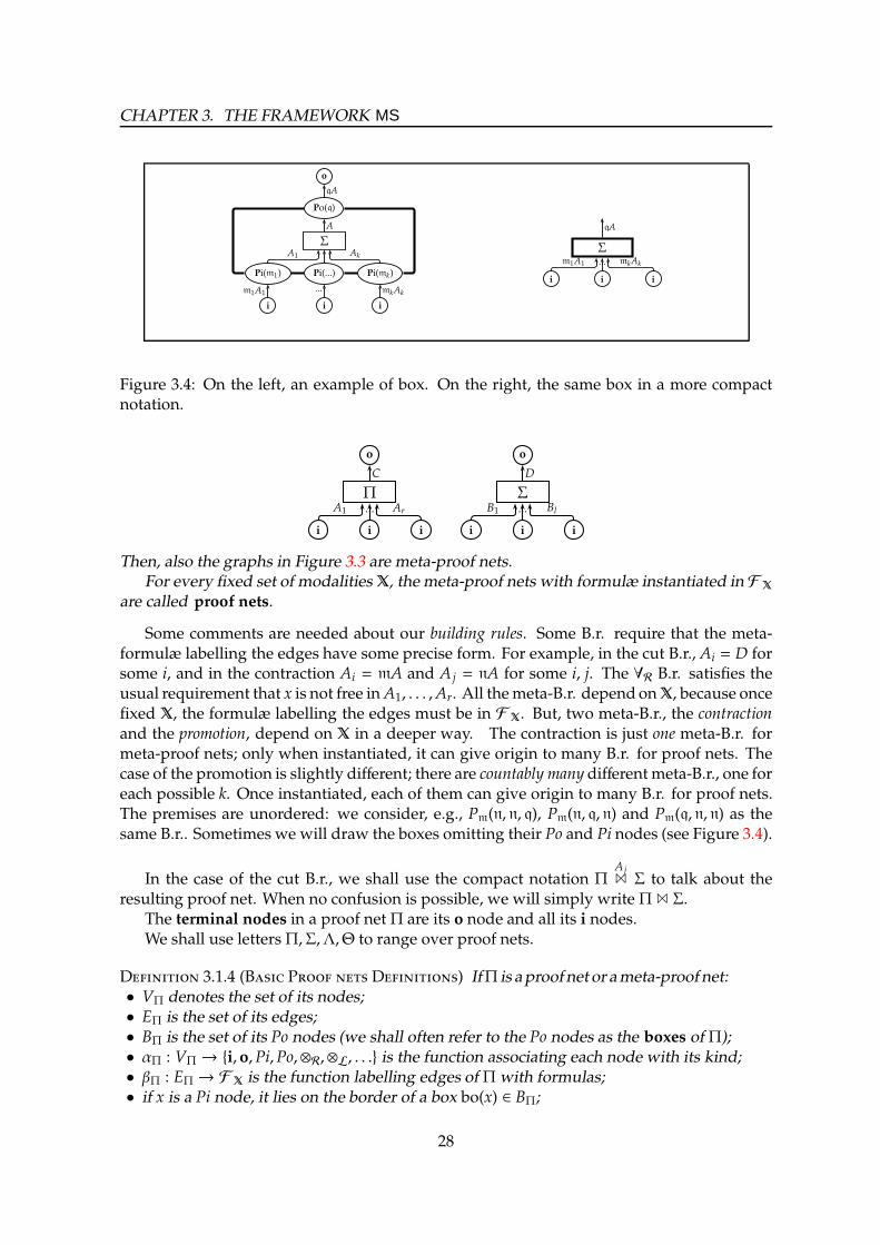
Figure 3.4: On the left, an example of box. On the right, the same box in a more compactnotation.
o o
Π Σ
i i i i i i
C D
A1 ... Ar B1 ... Bl
Then, also the graphs in Figure 3.3 are meta-proof nets.For every fixed set of modalities X, the meta-proof nets with formulæ instantiated in F X
are called proof nets.
Some comments are needed about our building rules. Some B.r. require that the meta-formulæ labelling the edges have some precise form. For example, in the cut B.r., Ai = D forsome i, and in the contraction Ai = mA and A j = nA for some i, j. The ∀R B.r. satisfies theusual requirement that x is not free inA1, . . . ,Ar. All themeta-B.r. depend onX, because oncefixed X, the formulæ labelling the edges must be in F X. But, two meta-B.r., the contractionand the promotion, depend on X in a deeper way. The contraction is just one meta-B.r. formeta-proof nets; only when instantiated, it can give origin to many B.r. for proof nets. Thecase of the promotion is slightly different; there are countably many different meta-B.r., one foreach possible k. Once instantiated, each of them can give origin to many B.r. for proof nets.The premises are unordered: we consider, e.g., Pm(n, n, q), Pm(n, q, n) and Pm(q, n, n) as thesame B.r.. Sometimes we will draw the boxes omitting their Po and Pi nodes (see Figure 3.4).
In the case of the cut B.r., we shall use the compact notation ΠA j
1 Σ to talk about theresulting proof net. When no confusion is possible, we will simply write Π 1 Σ.
The terminal nodes in a proof net Π are its o node and all its i nodes.We shall use lettersΠ,Σ,Λ,Θ to range over proof nets.
D 3.1.4 (B P D) IfΠ is aproofnet or ameta-proofnet:• VΠ denotes the set of its nodes;• EΠ is the set of its edges;• BΠ is the set of its Po nodes (we shall often refer to the Po nodes as the boxes of Π);• αΠ : VΠ → i, o,Pi,Po,⊗R,⊗L, . . . is the function associating each node with its kind;• βΠ : EΠ → F X is the function labelling edges of Π with formulas;• if x is a Pi node, it lies on the border of a box bo(x) ∈ BΠ;
28

3.1. META-PROOF NETS AND PROOF NETS
• PΠ : BΠ →N is the function telling how many premises has a box;
• boundary(Π)def= v ∈ VΠ | αΠ(v) ∈ i, o.
D 3.1.5 (P S I O) Let v be a node⊸L and ube a node⊸R as in figures:
⊸L
D
C⊸DC
⊸R
B
A⊸BA
The edge labelled C⊸ D is the principal input of v and the edge labelled C is the secondary(or auxiliary) input of v. The edge labelled A ⊸ B is the principal output of u, the edgelabelled A is the secondary (or auxiliary) output of u.
We call also reverse edge of u its secondary output.
R 3.1.6 Every proof net has a single conclusion: the system is intuitionistic.
R 3.1.7 Inside a proof net Π, boxes are in bijection with Po nodes.
D 3.1.8 (S A P ) If Π is a proof net with premises Γand conclusion C, we write
Π ⊲ Γ ⊢ C
and we say Γ ⊢ C is the sequent associated to Π, or that Π proves.
The latter definition is suggested by the usual correspondence between proof nets andsequent calculus.
hnodes and thehB.r. come directly from ILAL. They are necessary in handling reductionsof free weakenings, but they have not a meaningful corresponding rule in sequent calculus.
Finally:
D 3.1.9 MS is the set of all the meta-building rules. We will use labels that recallthe names of the B.r.:
MS =I, cut,h,W,⊗L,⊗R,⊸L,⊸R,∀L,∀R,Yq(m, n)
∪Pq(m1, . . . ,mk) | k ∈N
For each X, BX is the set of the building rules of MS instantiated with modalities in X.PN(BX) is the set of the proof nets built with the B.r. in BX.
BX =I, cut,h,W,⊗L,⊗R,⊸L,⊸R,∀L,∀R
∪
Yq(m, n) | m, n, q ∈ X
∪Pq(m1, . . . ,mk) | k ∈N, q,m1, . . . ,mk ∈ X
We will call linear kernel the set of all the non-modal B.r. in BX.
K =I, cut,h,W,⊗L,⊗R,⊸L,⊸R,∀L,∀R
29

CHAPTER 3. THE FRAMEWORK MS
Measures. We can now define the following measures on the proof nets.We shall use letters x, y, z, . . . to range over elements of VΠ ∪ EΠ.
D 3.1.10 Let Π be a proof net. For every x ∈ VΠ ∪ EΠ we define ∂(x), the depth (orlevel) of x:• If x ∈ VΠ, ∂(x) is the maximum number of (nested) boxes that contain x.
• If x = (u, v) ∈ EΠ, ∂(x)def= max ∂(u), ∂(v).
The depth of Π is ∂(Π)def= maxw∈VΠ ∂(w).
In particular, if u is a Pi or Po node, its depth is computed as u were outside the box it is onthe border of.
D 3.1.11 We denote VdΠthe set of nodes at dept d of Π. Similarly for Ed
Πand Bd
Π.
R 3.1.12 The terminal nodes only occur at level 0 of Π and P-nodes only at leveld < ∂(Π).
D 3.1.13 Let Π be a proof net.
• Its size is
|Π| = #nodes in Π, at every depth
.
• If 0 ≤ d ≤ ∂(Π), the size at level d ofΠ is
|Π|d = #nodes in Π, at depth d
This way,
|Π| =∑
0≤d≤∂(Π)
|Π|d.
We count every terminal node, every Pi-node and every Po-node as part of the size, forthey are part of our syntax. Lemma 3.4.4 and remark 3.4.5 will show that we could, in fact,harmlessly ignore them.
D 3.1.14 IfΠ is a proof net and 0 ≤ d ≤ ∂(Π), bd(Π) is the number of boxes at level
d.
Namely, this is the number of Po nodes. In particular b∂(Π)(Π) = 0.
L 3.1.15 (B R M)For every proof net Π and for every 0 ≤ d ≤ ∂(Π), bd(Π) ≤ |Π|d and bd(Π) ≤ |Π|d+1.
Proof. The first relation is trivial. For the second one, notice that every box contains at leastone node. 2
Figure 3.5 gives an example. In that proof net, ∂(Π) = 2, |Π|0 = 13, |Π|1 = 5 (rememberthat Pi and Po nodes are considered outside their box), |Π|2 = 1, and so |Π| = 22. The boxesare: b0(Π) = 3, b1(Π) = 1, b2(Π) = 0.
30
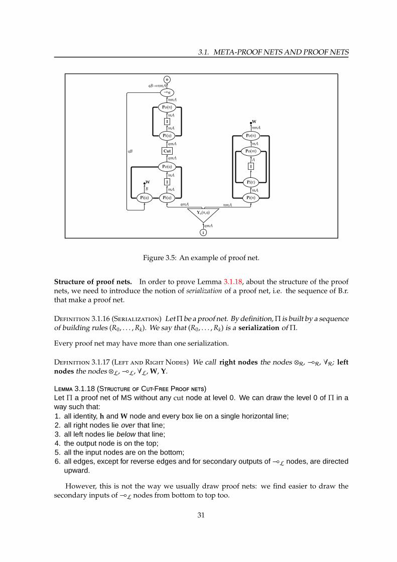
3.1. META-PROOF NETS AND PROOF NETS
o
⊸R
Po(n)
I W
Pi(q) Po(n)
Cut Po(m)
Po(q) I
W I Pi(r)
Pi(q) Pi(q) Pi(n)
Yq(n,q)
i
qB⊸nmA
mA
qB
qmA
nmAmA
mA
qmA A
B
mA
mA mA
nmA
qmA
qmA nmA
Figure 3.5: An example of proof net.
Structure of proof nets. In order to prove Lemma 3.1.18, about the structure of the proofnets, we need to introduce the notion of serialization of a proof net, i.e. the sequence of B.r.that make a proof net.
D 3.1.16 (S) LetΠ be a proof net. By definition,Π is built by a sequenceof building rules (R0, . . . ,Rk). We say that (R0, . . . ,Rk) is a serialization ofΠ.
Every proof net may have more than one serialization.
D 3.1.17 (L RN) We call right nodes the nodes ⊗R, ⊸R, ∀R; leftnodes the nodes ⊗L,⊸L, ∀L,W, Y.
L 3.1.18 (S C-F P )Let Π a proof net of MS without any cut node at level 0. We can draw the level 0 of Π in away such that:1. all identity, h and W node and every box lie on a single horizontal line;2. all right nodes lie over that line;3. all left nodes lie below that line;4. the output node is on the top;5. all the input nodes are on the bottom;6. all edges, except for reverse edges and for secondary outputs of⊸L nodes, are directed
upward.
However, this is not the way we usually draw proof nets: we find easier to draw thesecondary inputs of⊸L nodes from bottom to top too.
31

CHAPTER 3. THE FRAMEWORK MS
Proof. Π is built up thanks to a serialization (R0,R1, . . . ,Rn); it’s easy to prove the statementby induction on n, just looking back at the building rules of definition 3.1.3. 2
Subnets and Modules. In our work we shall use often the notion of module, i.e. a piece ofa proof net.
D 3.1.19 (M G) 1 Let Π be a proof net. Let us consider a subsetV ⊆ VΠ. The module Σ of Π generated by V is a boxed graph defined as follows.• All nodes in V are in VΣ.• If v ∈ V, α(v) ∈ Po,Pi, then Σ is the whole box bo(v).• If u, v ∈ V and (u, v) ∈ EΠ, then (u, v) ∈ EΣ.• If u ∈ V, v < V and (u, v) ∈ EΠ, then there exists an output node w ∈ VΣ, and an edge(u,w) ∈ EΣ.• If u ∈ V, v < V and (v, u) ∈ EΠ, then there exists an input node w ∈ VΣ, and an edge(w, u) ∈ EΣ.
D 3.1.20 (M) We call module a boxed graph Σ if there exist Π and V ⊆ VΠsuch that Σ is the module of Π generated by V.
An example is given in Figure 3.6. For each module Σ of Π there exists a canonical
injection iΣ : (VΣ\boundary(Σ)) → VΠ. When no confusion arises, if v ∈ VΣ we will writev ∈ VΠ meaning that iΣ(v) ∈ VΠ. Notice that a module is not necessarily connected.
R 3.1.21 (O NN) We shall use the notation Π ⊲Γ ⊢ ∆ meaning thatthe module Π has premises labelled with Γ and conclusions labelled with ∆. If Π ⊲ Γ,Φ ⊢ ∆and Σ ⊲ Γ′ ⊢ Φ,∆′ are two modules,Π 1 Σ ⊲ Γ, Γ′ ⊢ ∆,∆′ is the module obtained connectingΠand Σ through cut nodes, provided it is still a module. On the contrary, Π⊛Σ ⊲Γ, Γ′ ⊢ ∆,∆′
is the module obtained connecting Π and Σ just by edges, provided it is still a module.
D 3.1.22 (S) A subnet of Π is a module of Π that is also a proof net.
Environment subnets, surface graphs, paths. In this work, two notions of path will bedefined. The first one, here below, is similar to the standard notion of graph-theoreticalpath. The other one relates with a dynamical interpretation of the proof nets, and will bepresented in Section 4.3.1. Environment Subnets and Surface Graphs are objects required todefine graph-theoretical paths in a simple way.
D 3.1.23 Let us consider a proof netΠ and letΣ be amodule ofΠ. The environment
subnet of Σ is the largest proof net contained in the innermost box containing Σ, if it exists;it is Π otherwise.
This is also the largest subnet containing Σ and containing only nodes of depth ∂(x).In the following, if G is a graph, we use notation VG (resp. EG) for the set of nodes (resp.
edges) of G.
1Terminology comes from [DR89]
32
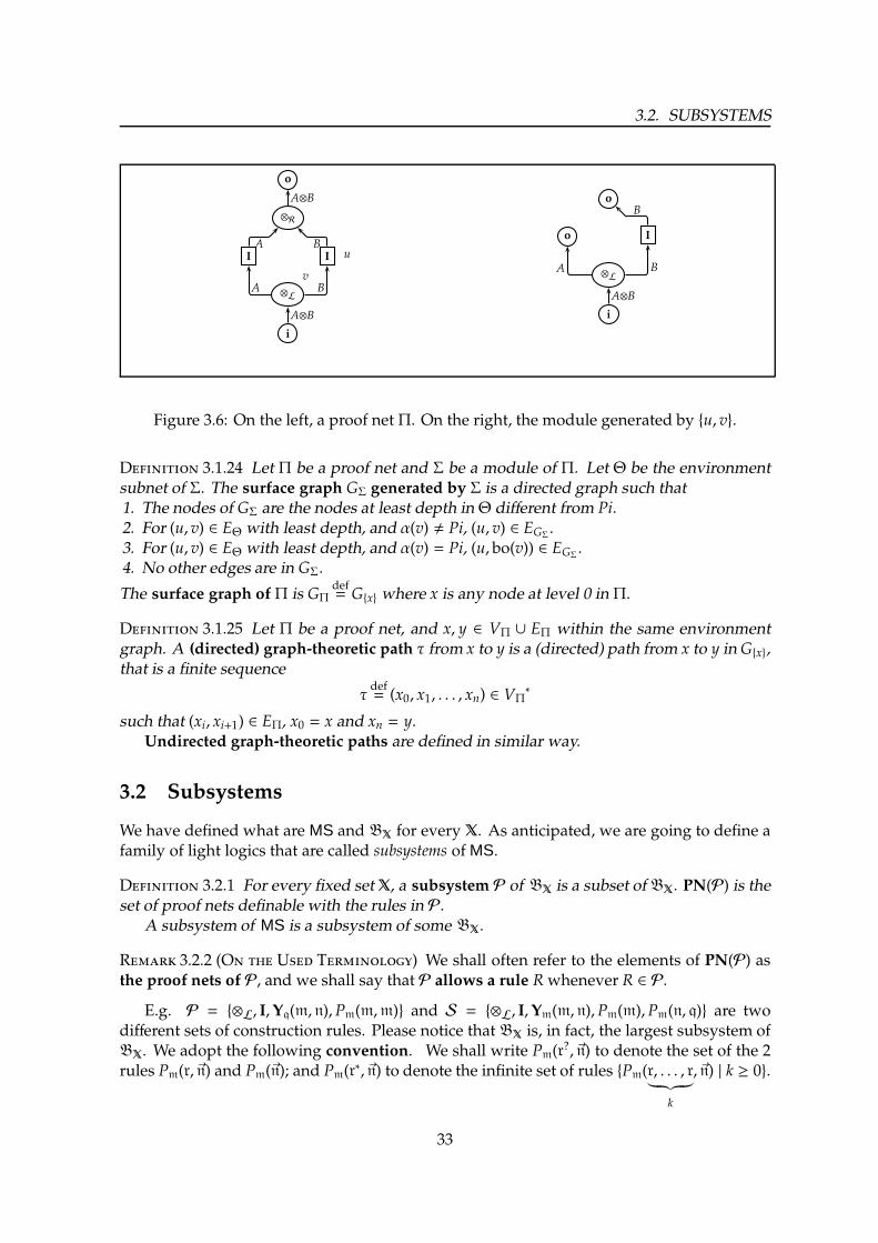
3.2. SUBSYSTEMS
o
⊗R
I I u
⊗L
v
i
A⊗B
A B
A B
A⊗B
o
o I
⊗L
i
B
A B
A⊗B
Figure 3.6: On the left, a proof net Π. On the right, the module generated by u, v.
D 3.1.24 Let Π be a proof net and Σ be a module of Π. Let Θ be the environmentsubnet of Σ. The surface graph GΣ generated by Σ is a directed graph such that1. The nodes of GΣ are the nodes at least depth in Θ different from Pi.2. For (u, v) ∈ EΘ with least depth, and α(v) , Pi, (u, v) ∈ EGΣ .3. For (u, v) ∈ EΘ with least depth, and α(v) = Pi, (u, bo(v)) ∈ EGΣ .4. No other edges are in GΣ.
The surface graph ofΠ is GΠdef= Gx where x is any node at level 0 in Π.
D 3.1.25 Let Π be a proof net, and x, y ∈ VΠ ∪ EΠ within the same environmentgraph. A (directed) graph-theoretic path τ from x to y is a (directed) path from x to y in Gx,that is a finite sequence
τdef= (x0, x1, . . . , xn) ∈ VΠ
∗
such that (xi, xi+1) ∈ EΠ, x0 = x and xn = y.Undirected graph-theoretic paths are defined in similar way.
3.2 Subsystems
We have defined what are MS and BX for every X. As anticipated, we are going to define afamily of light logics that are called subsystems of MS.
D 3.2.1 For every fixed setX, a subsystem P of BX is a subset ofBX. PN(P) is theset of proof nets definable with the rules in P.
A subsystem of MS is a subsystem of some BX.
R 3.2.2 (O U T) We shall often refer to the elements of PN(P) asthe proof nets of P, and we shall say that P allows a rule Rwhenever R ∈ P.
E.g. P = ⊗L, I,Yq(m, n),Pm(m,m) and S = ⊗L, I,Ym(m, n),Pm(m),Pm(n, q) are twodifferent sets of construction rules. Please notice that BX is, in fact, the largest subsystem ofBX. We adopt the following convention. We shall write Pm(r
?, ~n) to denote the set of the 2rules Pm(r, ~n) and Pm(~n); and Pm(r
∗, ~n) to denote the infinite set of rules Pm(r, . . . , r︸ ︷︷ ︸k
, ~n) | k ≥ 0.
33

CHAPTER 3. THE FRAMEWORK MS
D 3.2.3 Let P be a subsystem. We say it is downward closed iff whenever Phas Pm(m1, . . . ,mk), it has also all the rules Pm(mi1 , . . . ,mil) for every sublist (mi1 , . . . ,mil) of(m1, . . . ,mk).
For example, a subsystem without promotion rules is trivially downward closed.
D 3.2.4 Let X be the smallest set such that P ⊆ BX. We say that the number ofmodalities of P is #X.
In particular, whenever P ⊆ BX, P has at most #Xmodalities.
We will be interested in a particular class of subsystems:
D 3.2.5 P ⊆ BX is a sensible subsystem if:1. X is finite.2. P contains identity, cut and weakening.3. EitherX = ∅, or P contains at least one among⊸R and h.4. For every modality n∈X, P contains the closed box Pn().5. P is downward closed.
“Sensible” shortens computationally sensible subsystems, where we can erase/duplicate allthe structure wemight needwhenwriting proof nets-as-programs. Sensible subsystemswillbe relevant thanks to Proposition 4.3.40. Notice that, even if a subsystemP allows a rule R, ingeneral we are not sure that R can be really used inside some proof net. Think for example toP = I,Pm(n, q): a promotion rule with 2 premises cannot be used in any proof net of PN(P).If P is sensible, at least all its closed promotion rules can be really used:
F 3.2.6 (A D S)Point 3. in the Definition 3.2.5 can be equivalently replaced by the following:3bis. “For every n, the promotion rule Pn() can be used inside some proof net of PN(P).”
3.3 Normalization
Following the tradition of light logics, we are going to define a procedure of normalization forthe proof nets of MS. In Section 3.1 we have distinguished meta-proof nets and proof nets.Here, similarly, we distinguish between meta-normalization steps and normalization steps. Themeta-ns reduce meta-proof nets, while the ns reduce proof nets of every BX. Then, we willdefine also a normalization procedure for all the subsystems P of BX, restricting ad hoc thenormalization of BX.
The normalization tries to erase as many cuts as possible. For every X, we shall seethat BX (recall: BX is a subsystem of BX!) enjoys the cut-elimination property: it is possibleto normalize a proof net arriving to another proof net cut-free (Corollary 3.3.13). Thisproperty does not hold, in general, for the subsystems ofBX. This is why we adopt the termnormalization instead of the more traditional term cut-elimination.
D 3.3.1 Wewill call meta-normalization steps (or meta-ns) of MS all the rewritingrules in Figures 3.7, 3.8, 3.9, 3.10. The left side of a rule is the redex, the right-hand side isthe reduct.
34

3.3. NORMALIZATION
For every fixed setX, a normalization step (or ns) is a meta-nswith formulæ instantiatedin F X. R(BX) is the set of such ns.
Every ns has a name (e.g. [∀R/∀L], [W/P], . . . ).
D 3.3.2 For every fixed X, a normalization strategy σ is a function that takes aproof net of BX and tells which cut eliminating. Formally, σ : PN(BX)→ PN(BX), such that(i) Π→ σ(Π) or σ(Π) = Π, and (ii) if there is a reducible cut in Π then σ(Π) , Π.
Notice we do not require this function to be computable. We shall use letters σ, τ forstrategies.
In particular:
D 3.3.3 The closed normalization strategy requires that an instance of the modalcuts ([P/P] and [P/Y]) can be reduced only if the lowermost box they involve is closed.
D 3.3.4 (N) • If the proof net Π rewrites to Σ in a single ns, we writeΠ→ Σ.
• The transitive closure of→ will be denoted→∗.
• Π→n Σ iff Π→∗ Σ in exactly n steps.
• Π→σ Σ iff Π→∗ Σ using the strategy σ.
• Π→d Σ iff Π→ Σ reducing a cut node at level d.
• Π→S Σ iff Π→ Σ is a nswith name S.
• Combinations of the previous symbols shall be used.
D 3.3.5 A proof net Π is in normal form according to a strategy σ iff σ(Π) = Π. Aproof net is in normal form if it is in formal form according every possible strategy.
D 3.3.6 We will call normalization (resp. σ-normalization) of a proof net Π asequence of proof nets
〈Π = Π0,Π1, . . . ,Πn〉
where Πi → Πi+1 (resp. Πi →σ Πi+1), and such that Πn is in normal form.
L 3.3.7 (S R)Applying a ns to a meta-proof net leads to another meta-proof net. Applying a ns to a proofnet of BX leads to another proof net of BX.
Proof. The second statement is a consequence of the first one. So we prove just the first one.Given a meta-proof netΠ and one of its cuts u, the elimination of u using a single ns leads toanother boxed graph Π′. We want to showΠ′ is a meta-proof net.
The following is not a proof by induction; however it relies on the inductive definition ofproof net.
We will not prove the thesis for all possible cuts, just a relevant one.Let us consider u a cut [⊸R / ⊸L]. Π has been built, by definition, using some sequence
of construction rules Rij, as in Figure 3.11.
35
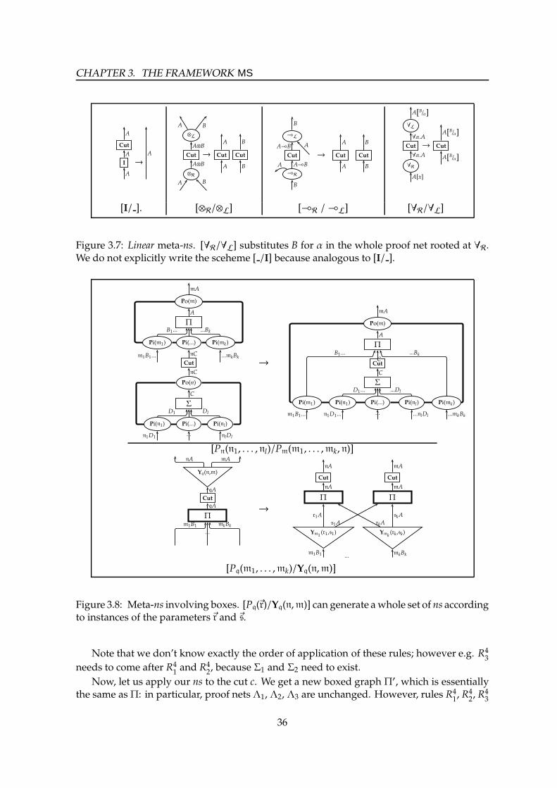
CHAPTER 3. THE FRAMEWORK MS
Cut
I →
A
A
A
A
⊗L
Cut → Cut Cut
⊗R
A B
A⊗BA B
A⊗B A B
A B
⊸L
Cut → Cut Cut
⊸R
B
AA⊸B
A⊸B
B
A B
A BA
∀L
Cut → Cut
∀R
A[B/α]
∀α.A
∀α.A
A[x]
A[B/α]
A[B/α]
[I/ ]. [⊗R/⊗L] [⊸R /⊸L] [∀R/∀L]
Figure 3.7: Linear meta-ns. [∀R/∀L] substitutes B for α in the whole proof net rooted at ∀R.We do not explicitly write the sceheme [ /I] because analogous to [I/ ].
Po(m)
Π
Pi(m1) Pi(...) Pi(mk)
Cut
Po(n)
Σ
Pi(n1) Pi(...) Pi(nl)
mA
A
B1... ...Bk
m1B1... nC ...mkBk
nC
C
D1 ... Dl
n1D1 ... nlDl
→
Po(m)
Π
Cut
Σ
Pi(m1) Pi(n1) Pi(...) Pi(nl) Pi(mk)
mA
A
C
C
B1...
D1... ... ...Dl
...Bk
m1B1... n1D1... ... ...nlDl ...mkBk
[Pn(n1, . . . , nl)/Pm(m1, . . . ,mk, n)]
Yq(n,m)
Cut
Π
nA mA
qA
qA
m1B1
...
mkBk
→
Cut Cut
Π Π
Ym1 (r1,s1) Ymk (rk,sk)
nA mA
nA mA
r1A
s1A rkA
skA
m1B1 mkBk...
[Pq(m1, . . . ,mk)/Yq(n,m)]
Figure 3.8: Meta-ns involving boxes. [Pq(~r)/Yq(n,m)] can generate awhole set of ns accordingto instances of the parameters~r and ~s.
Note that we don’t know exactly the order of application of these rules; however e.g. R43
needs to come after R41and R4
2, because Σ1 and Σ2 need to exist.
Now, let us apply our ns to the cut c. We get a new boxed graph Π′, which is essentiallythe same as Π: in particular, proof nets Λ1, Λ2, Λ3 are unchanged. However, rules R4
1, R4
2, R4
3
36
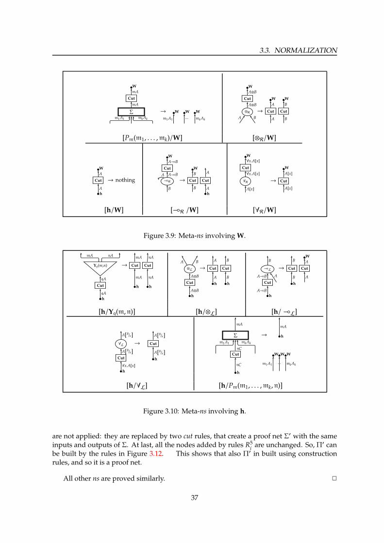
3.3. NORMALIZATION
W
Cut
Σ → W W W
mA
mA
m1A1 ... mkAk m1A1 ... mkAk
W
Cut W W
⊗R → Cut Cut
A⊗B
A⊗B A B
A B A B
[Pm(m1, . . . ,mk)/W] [⊗R/W]
W
Cut → nothing
h
A
A
W
Cut W
⊸R → Cut Cut
h
A⊸B
A⊸B
B
A B A
B A
W
Cut W
∀R → Cut
∀x.A[x]
∀x.A[x]
A[x]
A[x]
A[x]
[h/W] [⊸R /W] [∀R/W]
Figure 3.9: Meta-ns involving W.
Yq(m,n) → Cut Cut
Cut h h
h
mA nA
qA
qA
mA nA
mA nA
⊗L → Cut Cut
Cut h h
h
A B
A⊗B
A⊗B
A B
A B
W
⊸L → Cut Cut
Cut h
h
B
AA⊸B
A⊸B
B A
B A
[h/Yq(m, n)] [h/⊗L] [h/⊸L]
∀L → Cut
Cut h
h
A[B/x]
A[B/x]
∀x.A[x]
A[B/x]
A[B/x]
Σ → h
Cut W W W
h
mA
m1A1
nC
mkAk
mA
m1A1... mkAknC
[h/∀L] [h/Pm(m1, . . . ,mk, n)]
Figure 3.10: Meta-ns involving h.
are not applied: they are replaced by two cut rules, that create a proof net Σ′ with the sameinputs and outputs of Σ. At last, all the nodes added by rules R5
iare unchanged. So, Π′ can
be built by the rules in Figure 3.12. This shows that also Π′ in built using constructionrules, and so it is a proof net.
All other ns are proved similarly. 2
37

CHAPTER 3. THE FRAMEWORK MS
R11
R21
R31
. . . . . . . . .R1kis a rule R2
lis a rule R3
m is a rule
that creates that creates that createsΛ1 ⊲ Γ ⊢ A Λ2 ⊲ ∆,B ⊢ C Λ3 ⊲Θ,A ⊢ B
R41is a rule⊸Lthat creates R4
2is a rule⊸R
Σ1 ⊲ Γ,∆,A⊸ B ⊢ C that createsfrom Λ1 and Λ2. Σ2 ⊲Θ ⊢ A⊸ B
from Λ3.R43is a rule cut
that createsΣ ⊲ Γ,∆,Θ ⊢ Cfrom Σ1 and Σ2introducing c.
R51. . .
R5z creates Π
Figure 3.11: Proof of Stability Lemma.
R11
R21
R31
. . . . . . . . .R1kcreates R2
lcreates R3
m creates
Λ1 ⊲ Γ ⊢ A Λ2 ⊲ ∆,B ⊢ C Λ3 ⊲Θ,A ⊢ BR41is a rule cut
that createsΣ′1⊲ Γ,Θ ⊢ B
from Λ1 and Λ3.R42is a rule cut
that createsΣ′ ⊲ Γ,∆,Θ ⊢ Cfrom Σ1 and Λ2.
R51. . .
R5z creates Π
′
where rules R5iare the same rules R5
iapplied to a different proof net.
Figure 3.12: Proof of Stability Lemma.
38
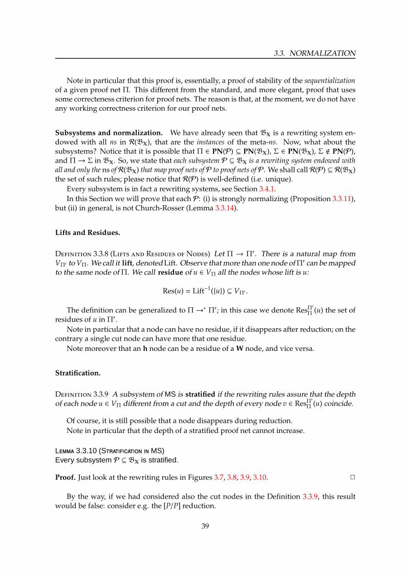
3.3. NORMALIZATION
Note in particular that this proof is, essentially, a proof of stability of the sequentializationof a given proof net Π. This different from the standard, and more elegant, proof that usessome correcteness criterion for proof nets. The reason is that, at the moment, we do not haveany working correctness criterion for our proof nets.
Subsystems and normalization. We have already seen that BX is a rewriting system en-dowed with all ns in R(BX), that are the instances of the meta-ns. Now, what about thesubsystems? Notice that it is possible that Π ∈ PN(P) ⊆ PN(BX), Σ ∈ PN(BX), Σ < PN(P),and Π→ Σ in BX. So, we state that each subsystem P ⊆ BX is a rewriting system endowed withall and only the ns of R(BX) that map proof nets ofP to proof nets ofP. We shall call R(P) ⊆ R(BX)the set of such rules; please notice that R(P) is well-defined (i.e. unique).
Every subsystem is in fact a rewriting systems, see Section 3.4.1.
In this Section we will prove that each P: (i) is strongly normalizing (Proposition 3.3.11),but (ii) in general, is not Church-Rosser (Lemma 3.3.14).
Lifts and Residues.
D 3.3.8 (L R N) Let Π → Π′. There is a natural map fromVΠ′ toVΠ. We call it lift, denotedLift. Observe thatmore than one node ofΠ′ can bemappedto the same node ofΠ. We call residue of u ∈ VΠ all the nodes whose lift is u:
Res(u) = Lift−1(u) ⊆ VΠ′ .
The definition can be generalized to Π →∗ Π′; in this case we denote ResΠ′
Π (u) the set ofresidues of u in Π′.
Note in particular that a node can have no residue, if it disappears after reduction; on thecontrary a single cut node can have more that one residue.
Note moreover that an h node can be a residue of a W node, and vice versa.
Stratification.
D 3.3.9 A subsystem of MS is stratified if the rewriting rules assure that the depthof each node u ∈ VΠ different from a cut and the depth of every node v ∈ ResΠ
′
Π (u) coincide.
Of course, it is still possible that a node disappears during reduction.
Note in particular that the depth of a stratified proof net cannot increase.
L 3.3.10 (S MS)Every subsystem P ⊆ BX is stratified.
Proof. Just look at the rewriting rules in Figures 3.7, 3.8, 3.9, 3.10. 2
By the way, if we had considered also the cut nodes in the Definition 3.3.9, this resultwould be false: consider e.g. the [P/P] reduction.
39

CHAPTER 3. THE FRAMEWORK MS
Basic properties of subsystems.
P 3.3.11 (E U B)For each d ∈ N there exists an elementary function ed(n) that bounds the reduction time ofall the proof nets Π ∈ PN(BX) with depth d and size n.
Vice versa, for every elementary function e(n) there exists a depth d and sequence ofproof nets Πn ∈ PN(BX) such that every Πn reduces in time ≥ e(n).
Proof. We can embed BX in IEAL just collapsing all the modalities n into !. It is well-knownthat IEAL reduces in elementary time.
Vice versa, it’s clear that every IEAL proof can be encoded in BX, using a particularmodality m instead of !. So BX is at least as expressive as IEAL. 2
C 3.3.12 (T)Every normalization terminates in a finite number of steps.
C 3.3.13 (C-)The subsystem BXenjoys the cut-elimination property.
Proof. Every cut can be reduced, using the ns of BX. Corollary 3.3.12 tells that everynormalization eventually terminates; hence the normal form must be cut-free. 2
On the contrary, Church-Rosser confluence property does not hold:
L 3.3.14 (N-D N)There are proof nets Σ, Π1, Π2 such that Σ→∗ Π1, Σ→∗ Π2, andΠ1 andΠ2 are two differentproof nets in normal form.
This is due to non-determinism in [Y/P] ns.
3.4 Technical considerations
3.4.1 Abstract Rewriting Systems
Here we will recall the definition of Abstract Rewriting System (ARS) from [Klo92, KBV01].Each subsystemP is in fact an instance of ARS. So, some (few) theorems holding for a genericARS also hold for P. We underline that, in literature, terms rewriting systems (TRS) are morewidely used than ARS. TRS are a particular case of ARS, whose objects are terms; but each Pis not a TRS, because its objects are proof nets instead of terms.
D 3.4.1 An Abstract Rewriting System (or ARS) is an algebraic structure A =
〈A,→〉 where A is a set and→ is a binary relation over A. ։ is the transitive and reflexiveclosure of→. ← is the inverse relation of←. և the transitive and reflexive closure of←. ≡is the convertibility relation: it is the smallest equivalence relation containing։. a ∈ A is anormal form (n.f.) if there is no b such that a→ b. a is a n.f. of b if a is a n.f. and b։ a.
(WCR) A is weakly Church Rosser if ∀a, b, c ∈ A (c← a→ b⇒ ∃d ∈ A (c։ dև b)) .
(CR) A is Church Rosser if ∀a, b, c ∈ A (cև a։ b⇒ ∃d ∈ A (c։ dև b)) .
40

3.4. TECHNICAL CONSIDERATIONS
(WN) A is weakly normalizing if every a ∈ A has a n.f.
(SN) A is strongly normalizing if every reduction a0 → a1 → . . . eventually terminates.
• A is complete if it is SN and CR.
(NF) A has the normal form property if ∀a, b ∈ A, a is a n.f. and a ≡ b implies b։ a.
(UN) A has the unique normal form property if ∀a, b ∈ A, a, b are n.f. and a ≡ b impliesa = b.
(FB) A is finitely branching if ∀a ∈ A there exist at most a finite number of b ∈ A such thata→ b.
If A = 〈A,→A〉 and B = 〈B,→B〉 are two ARS such that A ⊆ B, then:• B is a conservative extension of A if ∀a, a′ ∈ A (a→A a′ ⇔ a→B a′).• A is a substructure of B if, moreover, ∀a ∈ A∀b ∈ B (a→B b⇒ b ∈ A).
The following is proved as Theorem 1.0.7 in [Klo92]:
T 3.4.2 (B P ARS)1. CR⇒ WCR.2. SN⇒ WN.3. CR⇒ NF⇒ UN.4. SN + WCR⇒ CR.5. UN + WN⇒ CR.
Now, we apply the previous definitions and theorems to our subsystems. For every fixedX, the structure A = 〈PN(BX),→〉 is an ARS. If X is finite, such ARS is FB; indeed, everyproof net has a finite number of cuts, and each of them can reduce in a finite number of ways,being X finite. Moreover, A is SN (Corollary 3.3.12), but it is not WCR (Lemma 3.3.14), soneither CR.
For every P ⊆ BX, the structure B = 〈PN(P),→〉 is an ARS, too. A is a conservativeextension of B; however, B is not in general a substructure of A , because it is possible thatΠ ∈ PN(P) reduces – in BX – to some Π′ < PN(P). B is FB and SN (properties inherited byBX), but not in general WCR. Theorem 3.4.2 implies that whenever B is WCR it is also CR,and so it is also NF and UN. Summing up:
C 3.4.3 (B P S)For every P ⊆ BX, the structure B = 〈PN(P),→〉 is an ARS. B is SN. B is WCR if and onlyif it is CR; and if it is WCR it is also NF and UN. If X is finite, B is FB.
This property will be used in Section 5.2.
3.4.2 The definition of Size
In Section 3.1 we have defined the size of a proof netΠ as the number |Π| of nodes appearing init. This definition, apparently trivial, hides in fact some important issues. (i) All the premisesof a promotion box contribute to |Π|; but in fact the promotion is one single rule, both inthe sequent calculus or in the natural deduction formalisms. Similarly, the size includes also
41

CHAPTER 3. THE FRAMEWORK MS
the terminal nodes, i.e. premises and conclusion of the proof net, that do not correspond toany logical rule. We will prove that the premises of the box contribute to square the sizeof Π, that is: if N is the number of nodes in Π different from a Pi node or a terminal node,then |Π| = O
(N2)(Lemma 3.4.4). As a consequence, since we are only interested in the
polynomial time, the two definitions are equivalently good. (ii) |Π| does not consider the sizeof the formulæ appearing as label of Π. This is quite common in literature [AR02, Laf04];and indeed there is a deep reason in this choice. For example, in either ILAL or SLL, ifwe count also the time required to change the formulæ of Π, the reduction of Π cannot beperformed in polytime. Anywaywe shall see that the size of the formulæ has an impact onlyover subsystems that allow the second order quantification (Lemma 3.4.7 and 3.4.8). (iii) TheComputational Complexity is traditionally formulated in terms of Turing machines. Whatis the relationship between |Π| and the number of bits required to encode Π on the tape of aTuring machine? We will see that this last number is polynomial in |Π|.
L 3.4.4 (S T N)Given a netΠ, let s be its size, ∂ its depth, s its size without counting the terminal nodes, ands its size without any terminal node and any Pi node at any depth. Then
s = O(s);
s = O(∂ · s)= O(s2).
Proof. Let us call n(Π) the number of non-terminal nodes (including boxes) of Π at level0; t(Π) the number of terminal nodes (of course at level 0); N(Π) = s the number of non-terminal nodes at any depth; and T(Π) the number of terminal nodes and Pi nodes, at anydepth. n(Π) + t(Π) = |Π|0 while N(Π) + T(Π) = |Π|, and s = |Π| − t(Π).
We show by induction on ∂ that t(Π) ≤ 3N(Π).
(i) If ∂ = 0, there are no boxes; so each non-terminal node is connected to at most 3 nodes;and each terminal node is connected to some non-terminal node; so t(Π) ≤ 3N(Π).
(ii) Let ∂ > 0, and B = b0(Π). Inside the B boxes we find B subnets, which we can callΠ1, . . . ,ΠB, whose depth is less than ∂. We can consider the Pi nodes at level 1 as theterminal nodes ofΠ1, . . . ,ΠB. Now, N(Π) = N(Π1) + . . . +N(ΠB) + n(Π). Following theargument for the base-case,
t(Π) ≤ 3(n(Π)) + t(Π1) + . . . + t(ΠB)
≤ 3n(Π) + 3N(Π1) + . . . + 3N(ΠB) by inductive hypothesis
≤ 3N(Π).
This shows that t(Π) ≤ 3N(Π) = 3s, and s = s+ t(Π) = O(s). Now, we have to study T instead
of t. Again, by induction:
(i) If ∂ = 0, T(Π) = t(Π) ≤ 3N(Π) = 3 · 1 ·N(Π).
(ii) If ∂ > 0,
T(Π) = T (Π1) + . . . + T (ΠB) + t(Π)
≤ 3 · (∂ − 2) ·N (Π1) + . . . + 3 · (∂ − 2) ·N (ΠB) + 3N (Π)
≤ 3 · (∂ − 1) ·N(Π)
= 3 · (∂ − 1) · s.
42

3.4. TECHNICAL CONSIDERATIONS
And so s = N(Π) + T(Π) = O(∂ · s). 2
R 3.4.5 (A O T) The reason why we have proved Lemma 3.4.4 is thatwe were initially worried whether the theorems that we will prove in Chapter 4, and inparticular the Polynomiality Criterion 4.3.40, could not hold if we change the definition ofsize according to Lemma 3.4.4. The answer is yes, they still hold; the point is to use largerpolynomials.
On the size of the formulæ. Let us move to the second question: what about the size ofthe formulæ?
D 3.4.6 We suppose that a binary coding for formulas has been declared, and thelengths of the formulæ are calculated in bits. Given a proof net Π of MS, we will call γ(Π)the maximum length of formulas appearing on edges of Π.
L 3.4.7If Π is a net of MS, without any ∀ nodes. Then γ(Π) cannot increase during reduction.
Proof. Just look back at the ns: sometimes formulas disappear, sometimesmA is replaced bynA, but the size of formulas does not increase. 2
L 3.4.8Let X be fixed, and Π,Π′ ∈ PN(BX), such that Π→ Π′. Then γ(Π′) ≤ γ(Π)2.
Proof. The heavier case is that of [∀L/∀R]. Let us imagine we are eliminating the followingcut ofΠ:
Σ
∀L
Cut
∀R
Θ
A[B/α]
∀α.A
∀α.A
A
→
Σ
Cut
Θ[B/α]
A[B/α]
A[B/α]
In this case we have to change all the labels x in Π with another formula B, which couldbe larger. B is at most γ(Θ) ≤ γ(Π) long; and all other formulæ in Θ can contain at mostγ(Θ) ≤ γ(Π) occurrences of x; so γ(Π′) ≤ γ(Π)2. 2
So, if Π has O(n) cuts of kind [∀L/∀R], and they all are eliminable, after the reduction
γ(Π′) ≤ γ(Π)2O(n)
43

CHAPTER 3. THE FRAMEWORK MS
andΠ′ will require an exponential number of bits to be completely encoded. This is why wewill accept the tradition to ignore the length of the formulæ when encoding a proof net.
Relationship with Turing machines. In this last paragraph, we compare the size of a proofnet with the size of an encoding of the same proof net on the tape of a Turing machine. Aproof net Π is compounded of:• A graph VΠ of |Π| nodes and at most 3|Π| edges: it can be encoded using an adiacencymatrix (|Π|2 bits) or an incidence matrix (≤ 3|Π|2 bits), or a list of edges as couple of nodes(≤ 3|Π| · 2 log (|Π|) bits).• Some additional boxes, which are identified by their nodes: O(|Π|) nodes per each box, soO(|Π| · log (|Π|)
)bits.
• A label for each node, chosen among 15 different shapes: 4 · |Π| bits.• A label for each edge, which is an arbitrarily long formula. We can decide to ignore them,or to encode them using at most O(γ(Π)) bits each, and O
(|Π| · γ(Π)
)bits all.
So, without labels, the proof net can be codified by O(|Π| · log (|Π|)
)bits, and with labels
O(|Π| · log (|Π|) + |Π| · γ(Π)
)bits. It follows that |Π| is a good choice for the complexity of the
graph.
3.4.3 Why SLL is not a subsystem of MS
SLL, the Soft Linear Logic of [Laf04], is a polytime logic derived from LL. It has been brieflyrecalled in Section 2.4; it has the additive and multiplicative rules of LL, plus the exponentialrules reported in Figure 2.3, in a sequent calculus style. Our original targetwas the immersionof SLL into MS. That is, we wanted to find some subsystem P ⊆ MS and a compositionalembedding from proof nets of SLL into proof nets of P, such that every reduction in SLLcorresponds to a reduction in P, too. Notice that this target would be interesting, becauseSLL is not a stratified system, as it has the multiplexor rule.
The ideawas the following. Take a proof netΠ of SLL. Some new boxes have to be addedtoΠ; each multiplexor inΠwith n = 2 premises has to be transformed in a contraction, plustwo !-premises of some new box; if n > 2 the multiplexor will be replaced with an ad hocnumber of contractions; if n = 1 the multiplexor (or dereliction) has to be transformed into a!-premise of some new box.
However this is not possible, as the example in Figure 3.13 shows. The reader can try toadd some new boxes to this proof net; he will see that, if any box passes trough the lowerdereliction, then the two formulas labelling the premises of the lower multiplexor will bedifferent.
On the other side, it is possible to write SLL as a stratified system, allowing a moreliberalized use of the modalities; see e.g. [GRV]. We will return on this topic in Section 8.2.2.
44

3.4. TECHNICAL CONSIDERATIONS
o
⊗R
Po
⊗R
⊗R
I I I I
Y
⊗L
Pi Pi
⊗L
Y
Y
i
(!((α⊗β)⊗α))⊗β
α β
α
β
α
!α
βα
!α
β
!(!α⊗β)
!(!α⊗β)
!!(!α⊗β)
Figure 3.13: The counterexample described in Section 3.4.3.
45

CHAPTER 3. THE FRAMEWORK MS
46

Chapter 4
Polynomiality in MS
In this Chapter we study PMS, the class of the subsystems of MS whose reductions areperformed in polynomial time. A formal definition of polynomiality is given in Section 4.1.All the subsystems of MS are stratified; thus, we will begin our study generalizing the proofof strong polynomial time of ILAL (Section 4.2).
Then, we will provide some conditions that make a subsystem polytime or not polytime.These theorems are divided in two Sections: 4.3 and 4.4. The first one contains some“semantical” criteria for polynomial time, while the second one moves towards the more“syntactical” criteria. “Semantical” here means that they rely on the context semantics of theproof nets; while the “syntactical” criteria recognize the polynomiality of a subsystem “justlooking at its rules”.
The first criterion of the Chapter is Proposition 4.3.40. It tells that a sensible subsystemP is polytime if and only if its rules do not allow the construction of a dangerous spindle.The statement requires some definitions. We recall that a subsystem is sensible if it containsa minimum amount of rules, needed for basic programming (Definition 3.2.5). A spindleand a dangerous spindle are geometrical configurations that may occur inside proof nets(Definition 4.3.26 and Figure 4.4a). The notion of spindle relies on context semantics (CS);so in Section 4.3.1 and 4.3.2 we will recall the basics of CS. The Criterion is then proved inSection 4.3.3.
After that, wewill find out somemore properties equivalent to theCriterion. In particular,Proposition 4.4.5 tells that a subsystem P is polytime if and only if its augmented subsystemS(P) contains some specific rules. S(P) is defined as an extension ofP containing certain rulesderivable in P. Similarly, Proposition 4.4.15 assures that a subsystem is polytime if it doesnot contain certain rules, described by means of a relation among modalities R↑. Anotherinteresting result (Lemma 4.4.13) says that the question “Is P polytime?” is decidable, at leastin most of the practical cases. It should be clear that these last theorems do not mention at allthe CS. Figure 4.1 here below summarizes the main results of Sections 4.3 and 4.4. Bewarethat the results recalled in the Figure require a number of definitions that the reader can findin the appropriate Sections.
At last, in Section 4.5 we adapt (some of) the previous theorem to some non-sensible sys-tem. We are interested in particular in subsystems that use an infinite number of modalities,as we think that they are very natural in a theoretical perspective.
47
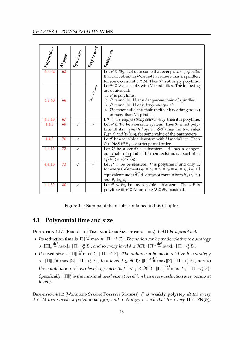
CHAPTER 4. POLYNOMIALITY IN MS
Proposition
Atpage
Syntactic?
Easyto
use?
Statemen
t
4.3.32 62 Let P ⊆ BX. Let us assume that every chain of spindlesthat can be built inP cannot havemore than L spindles,for some constant L ∈N. Then P is strongly polytime.
4.3.40 66 (sometim
es) LetP ⊆ BX sensible, withMmodalities. The following
are equivalent:1. P is polytime.2. P cannot build any dangerous chain of spindles.3. P cannot build any dangerous spindle.4. P cannot build any chain (neither if not dangerous!)
of more thanM spindles.4.3.43 67 IfP ⊆ BX enjoys strong determinacy, then it is polytime.4.4.5 69 X X Let P ⊆ BX be a sensible system. Then P is not poly-
time iff its augmented system S(P) has the two rulesPq(r, s) and Yq(r, s), for some value of the parameters.
4.4.8 70 X LetP be a sensible subsystemwithMmodalities. ThenP ∈ PMS iff R⋄ is a strict partial order.
4.4.12 72 X Let P be a sensible subsystem. P has a danger-ous chain of spindles iff there exist m, n, q such that
〈q〉R〈m, n〉R〈q〉.4.4.15 73 X X Let P ⊆ BX be sensible. P is polytime if and only if,
for every 6 elements q1 ≡ q2 ≡ r1 ≡ r2 ≡ s1 ≡ s2, i.e. all
equivalent under R↑,P does not contain both Yq1(r1, s1)and Pq2(r2, s2).
4.4.32 80 X Let P ⊆ BX be any sensible subsystem. Then, P ispolytime iff P ⊆ Q for some Q ⊆ BX maximal.
Figure 4.1: Summa of the results contained in this Chapter.
4.1 Polynomial time and size
D 4.1.1 (R T U S .) LetΠ be a proof net.
• Its reduction time is [Π]def= maxn | Π→n Σ. The notion can bemade relative to a strategy
σ: [Π]σdef= maxn | Π→n
σ Σ, and to every level d ≤ ∂(Π): [Π]ddef= maxn | Π→n
dΣ.
• Its used size is ‖Π‖def= max|Σ| | Π →∗ Σ. The notion can be made relative to a strategy
σ: ‖Π‖σdef= max|Σ| | Π →n
σ Σ, to a level d ≤ ∂(Π): ‖Π‖ddef= max|Σ| | Π →n
dΣ, and to
the combination of two levels i, j such that i < j ≤ ∂(Π): ‖Π‖j
i
def= max|Σ|i | Π →
∗jΣ.
Specifically, ‖Π‖j
iis the maximal used size at level i, when every reduction step occurs at
level j.
D 4.1.2 (W S P S) P is weakly polystep iff for everyd ∈ N there exists a polynomial pd(n) and a strategy σ such that for every Π ∈ PN(P),
48

4.1. POLYNOMIAL TIME AND SIZE
[Π]σ ≤ pd(|Π|).P is (strongly) polystep iff for every d ∈N there exists a polynomial pd(n) such that for everyΠ ∈ PN(P), [Π] ≤ pd(|Π|).
D 4.1.3 (W S P S) P is weakly polysize iff for everyd ∈ N there exists a polynomial pd(n) and a strategy σ such that for every Π ∈ PN(P),‖Π‖σ ≤ pd(|Π|).P is (strongly) polysize iff for every d ∈N there exists a polynomial pd(n) such that for everyΠ ∈ PN(P), ‖Π‖ ≤ pd(|Π|)).
D 4.1.4 (W S P S) P is (strongly) polytime iff it is bothstrongly polystep and strongly polysize.P is weakly polytime iff it is both weakly polystep and weakly polysize, under the samestrategy σ.
R 4.1.5 (A D P S) Ourdefinitionof polytime systemneedssome comments. Why is it necessary to consider different polynomials pd(n) when depthchanges? Let us consider two alternative definitions, each one based on the attempt to useone only polynomial:
1. P is weakly polynomial iff there exists a strategy σ and a polynomial p(n) such thatevery σ-normalization of a proof net Π takes at most p(|Π|) steps.
This is not so interesting, because P cannot codify all polytime functions.
2. P is weakly polynomial iff there exists a strategy σ such that for every proof Π of Pthere exists a polynomial pΠ(n) such that the σ-normalization ofΠ takes at most pΠ(|Π|)steps.
This is uninteresting, as well, because every system would be weakly polynomialaccording to every strategy σ, just choose pΠ(n) large enough.
Now, let us arrive to the main problem.
P 4.1.6 Given a system P ⊆ MS, is it (strongly) polynomial? or weakly polynomial?
Of course, for each X, BX is not polynomial, because of Proposition 3.3.11 at page 40.
D 4.1.7 PMS is the class of the subsystems of some BX that are polytime.
The following Lemma is a trivial property that we will use often:
L 4.1.8 (M)Let P ⊆ Q be two subsystems, and Q ∈ PMS. Then, P ∈ PMS, too.
Proof. All the reductions Π →∗ Σ that can be performed in P may be performed in Q, too.Now, inQ there exists a polynomial p(x) such that [Π], ‖Π‖ ≤ p (|Π|), and the same polynomialbounds the reductions in P. 2
49

CHAPTER 4. POLYNOMIALITY IN MS
R 4.1.9 (C B D) Some authors (e.g. [NM02]) underline that therewriting rules have not all the same cost (where the cost of a single ns is the time needed toperform it): box duplication should take a time proportional to the content of the box itself.Actually we agree with them, but for sake of simplicity we considered box-duplication asconstant-time.
4.2 Following ILAL
First of all, we generalize the proof of polynomial soundness for ILAL [AR02]. We classifythe cuts in Figures 3.7, 3.8, 3.9, 3.10 in the following way:
D 4.2.1 (C C) We call modal cuts the cut nodes named [P/P],[P/Y] and [I/ ]; linear cuts the cut nodes named [⊗/⊗], [∀/∀], [⊸ /⊸] and [I/ ]; and garbage
collector cuts (gc) the cuts [W/ ], [ /h] and [I/ ].
We notice that:1. The [I/ ] cuts belong to all the categories.2. The linear cuts can always be eliminated, in every systemPwhere they exist; eliminating
them at some level i can lead to some new cuts at the same level i, of unknown name.3. The elimination of a (reducible) modal cut can lead to some new modal cut or gc cut at
the same level (plus some other cuts at the higher levels).4. The elimination of a (reducible) gc cut can only lead to some new gc cut at the same level.These observations allow the following definition:
D 4.2.2 (C S) A reduction of Π is said canonical if it has thefollowing shape:
Π = Π0 →∗ Π′0 →
∗ Π1 →∗ Π′1 →
∗ . . .→∗ Π′∂ →∗ Π∂+1 →
∗ Σ
where ∂ = ∂(Π), Π′iis obtained reducing all the linear cuts at level i in Πi, Πi+1 is obtained
reducing all the modal cuts at level i inΠ′iand Σ is obtained reducing all the gc cuts inΠ′
∂+1.
L 4.2.3 (C S A T W O)Let Π be a proof net. For every reduction σ : Π = Π0 → Π1 → . . . → Πl = Σ there existsa canonical reduction τ : Π = Π′
0→ Π′
1→ . . . → Π′
l′= Σ such that (i) l′ ≥ l and (ii)
max|Π′i| | i ≤ l′ ≥ max|Π j| | j ≤ l.
Moreover, if σ is a reduction performed in some P ⊆ MS, then also τ is performed in P.
Proof. Weproceed by induction on l. If l ≤ 1, of course the reduction is canonical. Otherwise,we can assume that Π0 → . . . → Πl−1 can be transformed into some canonical reductionΠ = Π′
0→ Π′
1→ . . . → Π′
k= Πl−1, while Πl−1 →α Πl does not follow this canonical
reduction. The reduction of α does not follow a canonical reduction because there is another(reducible) cut β that should be reduced before α. We claim that we can reduce β before α,with some further minor modifications in the reduction sequence. Let us distinguish somecases:
1. α is a modal cut and β a linear cut at the same level. This case is easy: α and β do notinteract at all with each other (they are not a critical pair), so there is no difference inthe order of their reduction. We exchange them, and we build a new sequence, withthe same length l′ = l and with the same greatest size.
50
4.2. FOLLOWING ILAL
2. α is a gc cut and β a modal or linear cut. We can exchange the order of the 2 cuts. Now,it’s possible that some new reducible cuts appear, because according to σ it was erasedbefore reduction; we just reduce them and we get a new sequence with l′ ≥ l. The newsequence has the same greatest size than the previous one.
3. α has depth d′ and β has depth d < d′. Let us call b the box at level d in which α iscontained. Let us consider the possible β’s.
• Of course, if β is not a cut with b, we can just exchange α and β.
• Similarly if β is [P/P] with the box b.
• If β is [P/Y] with the box b, we can reduce β before α: in this way b is duplicated.The new normalization sequence is strictly longer than before, l′ > l. Moreoverthe greatest size of this new sequence can be greater than the greatest size of theprevious one.
2
L 4.2.4 (A C P)Let P ⊆ MS. Let us assume that for every ∂ there exist two polynomials p(x), q(x) such thatfor every proof net Π of P with ∂(Π) ≤ ∂ and for every d ≤ ∂(Π):
[Π]d ≤ p(|Π|), ‖Π‖d ≤ q(|Π|).
Then P is strongly polytime.
Proof. We prove that the result holds for every canonical reduction; Lemma 4.2.3 tell us thatin fact it holds for every reduction.
Let us consider a canonical reduction σ:
Π = Π0 →∗ Π′0 →
∗ Π1 →∗ Π′1 →
∗ . . .→∗ Π∂+1 →∗ Σ.
Π′iis obtained from Πi in linear time |Πi|, and the size is not increased: |Π′
i| ≤ |Πi|.
Πi+1 is obtained from Π′iin time p(|Π′
i|), and the size is at most |Πi+1| ≤ q(|Π′
i|).
Σ is obtained from Π∂+1 again in linear time |Π∂+1|, and the size does not increase:|Σ| ≤ |Π∂+1|. So
|Πi| ≤ q(|Π′i−1 |
)≤ q (|Πi−1|) ≤ q
(q (|Πi−2 |)
)≤ . . . ≤ q(i) (|Π|) ≤ q(∂) (|Π|) .
This means that P is polysize. Moreover, the reduction takes at most
|Π0| + p(|Π′0|)+ |Π1| + p
(|Π′1|)+ . . . + p (|Π∂|) + |Π∂+1|
≤ |Π0| + |Π1| + . . . + |Π∂+1| + p(|Π′0|)+ p(|Π′1|)+ . . . + p (|Π∂|)
≤ (∂ + 2) q(∂) (|Π|) + (∂ + 1) p(q(∂) (|Π|)
)
steps, and so P is also polystep. 2
This proof of weak polynomiality is a generalization of (part of) the proof of weakpolynomial soundness for ILAL in [AR02]. The proof of strong polynomiality is a variation ofthe proof of strong polynomiality for ILAL in [Ter07], but with a more combinatorial flavour.
51

CHAPTER 4. POLYNOMIALITY IN MS
4.3 Semantical Criteria for Polytime Soundness
The first propositions that we shall prove to distinguish polytime and not polytime subsys-tems P are semantical, in the sense that they are based on the context semantics of the proofnets of P.
4.3.1 Context semantics: definitions
We adapt the context semantics technology of [DL08]. Context semantics essentially definesa notion of CS-path over the nodes of a proof net. A CS-path between two nodes tells thatthey can communicate each other. For example, let us imagine that a proof netΠ contains twonodes u, v, one⊗L and the other one⊗R, and that during some reductionΠ→∗ Π′ the residuesu′, v′ of u, v become connected through a cut, so that they can finally annihilate. In this case,the context semantics says that, in Π, there is a CS-path between u and v. So, CS-paths canbe used to predict the future reductions of a proof net. Technically, CS-paths are obtainedusing contexts, that is quadruples (e,U,V, b), that record the nodes already encountered overa CS-path. We will describe them in a moment.
We just stress that our framework is simpler, since digging and dereliction are missing inMS. The first consequence is that we can use contexts (e,U, b) with just three components.Though, our version of context semantics must supply a quantitative computational modelfor systems where (i) the full cut-elimination does not hold, and (ii) the weakening is onarbitrary formulæ.
D 4.3.1 (E S) An exponential signature is a formula gener-ated by the following grammar:
tdef= e | r(t) | l(t).
E is the set of exponential signatures.
D 4.3.2 (S) A stack element is an element of Sdef= a, o, f, s, x ∪ E. A stack is
a finite non empty sequence of stack elements, that is an element s ∈ S+.
D 4.3.3 (P) A polarity is an element of Bdef= +,−. If c is a polarity, we
denote c ↓ the other one. When needed, we can consider the two polarities as ±1.
D 4.3.4 (C) LetΠ a proof net. Then a context ofΠ is an element of
CΠdef= EΠ × S+ × B.
The nodes of MS induce rewriting rules over contexts:
D 4.3.5 (R RA C) Let Π be a proof net, C,C′ ∈ CΠ.We write C 7→Π C′, if C′ can be obtained from C through the rewriting relation described inFigure 4.2.
52

4.3. SEMANTICAL CRITERIA FOR POLYTIME SOUNDNESS
⊸R
he
g
(g,U,+) 7→Π (h,U · o,+)
(e,U,−) 7→Π (h,U · a,+)
(h,U · o,−) 7→Π (g,U,−)
(h,U · a,−) 7→Π (e,U,+)
⊸L
h
eg
(g,U,+) 7→Π (e,U · a,−)
(h,U,−) 7→Π (e,U · o,−)
(e,U · a,+) 7→Π (g,U,−)
(e,U · o,+) 7→Π (h,U,+)
⊗R
h
e g
(e,U,+) 7→Π (h,U · f,+)
(g,U,+) 7→Π (h,U · x,+)
(h,U · f,−) 7→Π (e,U,−)
(h,U · x,−) 7→Π (g,U,−)
⊗L
e g
h
(h,U · f,+) 7→Π (e,U,+)
(h,U · x,+) 7→Π (g,U,+)
(e,U,−) 7→Π (h,U · f,−)
(g,U,−) 7→Π (h,U · x,−)
∀R
g
e
(e,U,+) 7→Π (g,U · s,+)
(g,U · s,−) 7→Π (e,U,−)
∀L
g
e
(e,U · s,+) 7→Π (g,U,+)
(g,U,−) 7→Π (e,U · s,−)
Yc(a,b)
e g
h
(h,U · l(t),+) 7→Π (e,U · t,+)
(h,U · r(t),+) 7→Π (g,U · t,+)
(e,U · t,−) 7→Π (h,U · l(t),−)
(g,U · t,−) 7→Π (h,U · r(t),−)
I
g
e
or Cut
g
e
(e,U,+) 7→Π (g,U,+)
(g,U,−) 7→Π (e,U,−)
Po(q)
Σ
Pi(m1) ...
. . .
h
l
gg
e
(e,U,+) 7→Π (h,U,+)
(h,U,−) 7→Π (e,U,−)
Figure 4.2: Rewriting Relation among contexts. Notice that if (e,U, b) 7→Π (e′,U′, b′) then also(e′,U′, b′ ↓) 7→Π (e,U, b ↓).
D 4.3.6 (C, I, F C) (e, t · U, b) is canonical if t is an ex-ponential signature, U does not contain exponential signatures, and if U contains an evennumber of a’s, then b is +, otherwise, if U contains an odd number of a’s, then b is −.(e, t,+) is initial if it is canonical and t is exponential.((u, v), e ·U, b) is final if it is canonical, and either
1. b = + and α(v) ∈ W, o, or
2. b = − and α(v) = i.
Canonical, initial and final contexts are the atomic steps that we use to compose the correctCS-paths to travel along the edges of a proof net. “Correct” means that a CS-path highlightsthe pairs of nodes that, eventually, will interact by means of a cut-elimination step, in thecourse of the normalization. The ultimate goal of defining CS-paths is to use them forwalking through a net from the root of any box to either a weakening node that will eraseit, or to a terminal node of the whole net or of a proof net inside a box. The existence ofmany canonical CS-paths from the same box root means the existence of contraction nodesthat, in principle, will duplicate the box. In particular, any initial context is defined to go
53

CHAPTER 4. POLYNOMIALITY IN MS
upward — thanks to its positive polarity — in the proof net, traversing contraction nodes —thanks to its exponential signature —. Any final context says that, starting from the root of abox, we have walked through a net “consuming” all the directions settled by an exponentialsignature, getting to the empty exponential signature e. Figure 4.3 is an example of completeCS-path from the root of the rightmost box to the output of the net, only highlighting thestack and the polarity. The leftmost box is “skipped” by the sequence of contexts associatedto the net, because we are in a stratified setting.
Recall that we have defined graph-theoretical paths on page 33. As anticipated, thefollowing is a different notion of path:
D 4.3.7 (CS-P M CS-P) Let Π ∈ PN(BX), b ∈ VΠ a Po node ora contraction, v ∈ VΠ. A CS-path from b to v is a finite sequence
τdef= (u0, u1 . . . , un−1, un) ∈ VΠ
∗
of nodes in Π, where b = u0 and v = un, for which there is a sequence of contexts
Tdef= (((b, u1),U0, b0), . . . , ((un−1, v),Un−1, bn−1)) ∈ CΠ
∗
such that (i) ((b, u1),U0, b0) is initial, and (ii) (ei,Ui, bi) 7→Π (ei+1,Ui+1, bi+1), for every 0 ≤ i ≤n − 1.
Moreover, τ is maximal if ((un−1, v),Un−1, bn−1) is final.Finally, we call T the sequence of contexts associated to τ.
Please notice that, differently from [DL08], a CS-path is made up of nodes, and not ofcontexts. This implies that two CS-paths are equal when they pass through the same nodes,regardless their contexts.
The definition of maximal CS-paths confirms the intuition given before. Every of themstarts from the root of a box b and shows where the root of a copy of b will eventually occur,after every instance of the rules only in Figures 3.7, and 3.8 have been applied.
Notice that an initial context is canonical, as well as all the contexts in a CS-path arecanonical.
A CS-path is not, in general, a graph-theoretical CS-path, because of the orientation ofedges.
D 4.3.8 (CS-P L) If τ = (u0, u1, . . . , un) is a CS-path, the length of τ is
len(τ)def= n.
D 4.3.9 (C) A cycle is a CS-path τ such that, if ((ei,Ui, bi))i≤n is its associatedsequence of contexts, then e0 = en and b0 = bn. A proof net is acyclic if it has no cycles.
D 4.3.10 (CS-P, N CS-P) Let Π ∈ PN(BX), b ∈ BΠ. Then
OΠ(b)def=τ | τ is a maximal CS-path from b to some v ∈ VΠ
.
RΠ(b)def= #OΠ(b).
54

4.3. SEMANTICAL CRITERIA FOR POLYTIME SOUNDNESS
o
I
⊸L
⊸L
Cut I I
⊸R Y
⊸R Cut
Po Po
I ∀R
⊸L Π
∀L I
Pi Pi
(e,+)
(e,+)
(e a,−)(e o,+)(e,+)
(e ao,−)(e oo,+)
(e ao,−)(e oo,+) (e,+)
(e a,−)(e o,+) (r (e),+)
(e,+) (r (e),+)
(e,+)
Figure 4.3: An example of maximal path.
Like in [DL08] we call RΠ(b) the number of copies of b. The expression “number ofcopies” anticipates the content of Lemma 4.3.16: RΠ(b) shall give a bound on the number ofcopies of b that can be generated during a reduction. This is the content of
D 4.3.11 (P W) Let Π be a proof net. Its weight at depth d ≤ ∂(Π) is
Wd(Π)def=∑
b∈BdΠ
RΠ(b).
D 4.3.12 (P MW) Let Π be a proof net. Its modified weight
at depth d ≤ ∂(Π) is
Td(Π) =∑
u∈VdΠ
Td(Π, u)
Td(Π, u)def=
1 α(u) ∈ I, cut,W,h,Pi(m), i, o
3 α(u) ∈ ⊗L,⊗R,∀L,∀R,⊸L,⊸R,Yq(m, n)
2 · (PΠ(u) + 1) · RΠ(u)2 α(u) ∈ Po(m).
55

CHAPTER 4. POLYNOMIALITY IN MS
(PΠ was defined on page 28). Notice that this weight is slightly simpler than the onedefined in [DL08]. Again, the simplification is possible thanks to the stratification of oursetting.
4.3.2 Properties of the Context semantics
We show that themain properties of the context semantics, as proved in [DL08], keep holdingin our setting, in which, we recall, we have unconstrained weakening and, for any genericP of MS, we cannot assure full cut elimination. Recall, indeed, that cut elimination holdsfor each full BX; so, in all the following proofs, we will imagine that the reductions areperformed in BX, instead than in particular P ⊆ BX.
In order to simplify our proofs, we firstly print some properties (from Remark 4.3.13 upto Lemma 4.3.15) that do not hold in the generalCS settings, but only in our specific stratifiedsetting.
R 4.3.13 (R CS- .) If (e, t·U, b) is a canon-ical context in a CS-path τ, the top of the stack t · U relates to the formula β(e) that labelse. If β(e) is A ⊗ B, then the top is f or x. Similarly, β(e) = ∀α.A corresponds to the s, whileβ(e) = A ⊸ B to one between o and a. Finally, if β(e) = nA, the top element must be theexponential signature t.
R 4.3.14 (S R U) We remark that, thanks to what we have just un-derlined, the canonical contexts inside a CS-path τ can never reach neither a Po node, nor a Ynode with negative polarity. Indeed, a negative polarity implies that at least one a is presenton the stack, while the context of an edge incident in a contraction or Po node has t as stack.As a consequence, 3 of the the rewriting rules from contexts to contexts are useless: theyare the three rules that arrive to nodes Po,Y with negative polarity. Also, a CS-path onlyconsumes an (initial) exponential signature, never adding l or r symbols.
In traditional CS, composition of CS-paths is not in general a CS-path. Instead, with ourlimited notion of CS, the property holds:
L 4.3.15 (C CS-P CS-P)Let τ be a CS-path from u to v inside some proof netΠ, where v is a Po or a contraction; andσ be a CS-path from v to w. Then, the path obtained joining τ and σ is still a CS-path.
Proof. The CS-path τ starts in uwith context (e1, t1,+) and arrives in vwith context (e2, t2,+).The CS-path σ starts in v with context (e3, t3,+) and arrives in w with context (e4, t4,+). Wepointed out that τ cannot add new exponential signatures to t1; so t1 = T(t2). So, t2 isuntouched and we can freely replace it with t3. We have found another different sequence ofcontexts for τ: it starts in u with context (e1,T(t3),+) and arrives in v with context (e2, t3,+).This sequence of context may go on up to w following the contexts for σ. So we found asequence of CS-paths for the composition of τ and σ. 2
The following Lemma explains the meaning of the expression “number of copies”.
L 4.3.16 (N C)Let Π→∗
dΣ, b ∈ Bd
Πand Θ the proof net inside b at depth d+ 1. Then, in Σ, there are at most
RΠ(b) equal residues (“copies”) of Θ.
56

4.3. SEMANTICAL CRITERIA FOR POLYTIME SOUNDNESS
D 4.3.17 LetΠ reduce toΣ in a single ns, byfiring a cut c. Also, let τ = (u0, . . . , ui−1, c, ui+1, . . . , un)be a CS-path in Π that passes by c. The residue Res(τ) of τ is the set of the residues of thenodes of τ in Σ.
L 4.3.18 (T R CS-P CS-P)Let Π → Σ through the reduction of a cut c. Let τ = (u0, . . . , ui−1, c, ui+1 . . . , un) be a CS-pathin Π that passes by c. The residue Res(τ) of τ, ordered in the natural way, is still a CS-path.
Proof. The proof is by cases on the possible ns. 2
One may imagine to relax the Definition 4.3.17 allowing the path τ not passing by c.However in this case Lemma 4.3.18 would be false: think to the [h/P] ns, where the residueof a path may be disconnected.
On the other side, every CS-path in Σ is the residue of – at least – one CS-path in Π; wecall Φ the relation that associates a CS-path in Σ with all the corresponding CS-paths in Π.Φ is not, in general, a function.
L 4.3.19Every proof net Π is acyclic.
Proof. Let us consider a canonical reduction forΠ:
Π = Π0 → Π1 → . . .→ Πn →∗ Σ
where n has been chosen least (please see on page 50 the definition of canonical strategy).We proceed by induction on n.
Base case. n = 0 means Π contains only gc cuts. Straightforward to prove, by induction onthe structure ofΠ, that if (e,U, b) 7→+
Π(e,V, c) then b , c.
Inductive case. If Π →S Π1, by inductive hypothesis we can assume Π1 is acyclic. Now,every CS-path τ in Π corresponds to (at least) CS-path Φ(τ) in Π1, as we have alreadysaid; and the correspondence Φ preserves acyclicity. 1
2
L 4.3.20For each Π and b ∈ BΠ, RΠ(b) ≥ 1.
Proof. Let us consider a sequence of contexts starting from a box b with a context (e, t,+),where t is an exponential signature. Provided t is long enough, there is no way to stop sucha sequence, unless (i) we arrive in a W, i or o node, or (ii) the CS-path is a cycle and returnsat the starting point. But this second situation is forbidden by the previous lemma. So thereis at least a canonical sequence of contexts starting from b and arriving in a W, i or o node.Choosing t of the correct size, we can make the last context a final context, and this is amaximal CS-path. 2
1This latter observation would not be obvious if S were a gc step.
57

CHAPTER 4. POLYNOMIALITY IN MS
L 4.3.21If Π at level d has only gc and [P/P] cuts, then for every b ∈ BΠ, RΠ(b) = 1.
Proof. By structural induction onΠ. 2
L 4.3.22 (Wd Td D)Given a proof net Π, let us suppose Π→S Σ. Then
1. Wd(Π) =Wd(Σ), if S ∈ [⊸ /⊸], [⊗/⊗], [∀/∀], [P/Y];
2. Wd(Π) =Wd(Σ) + RΠ(b), if S = [P/P] and b is one of the merged boxes;
3. Wd(Π) ≥Wd(Σ), if S is a gc step;
4. Td(Π) > Td(Σ);
Proof. In the first case the CS-paths and the boxes are untouched, so for every b, RΠ(b) =RΣ(Res(b)). In the second case, a box b disappears, so the sum that defines Wd decreases ofexactly RΠ(b). In the third case, also, a box may disappear depending on what kind of nodeis cut with the weakening node.
For the last point, the reader can check that Td(Π) strictly decreases for every possiblereduction step; we only prove the most difficult case. Let us assume Π →S Σ by a [P/Y]normalization step; a box b is duplicated in b1, b2. Let P = PΠ(b) = PΠ(bi) and Ri = RΠ(bi); itholds RΠ(b) = R1 + R2. Now, if we call x the weight of a generic contraction, y the weight ofa cut, and z the weight of a Pi node,
Td(Π) = A + x + y + Td(b) + P · z
= A + 3 + 1 + 2(P + 1)(R1 + R2)2 + P
Td(Σ) = A + 2y + Td(b1) + Td(b2) + 2P · Td(a Pi) + P · x
= A + 2 + 2(P + 1)R21 + 2(P + 1)R2
2 + 2P + 3P.
Td(Π) − Td(Σ) = 2 + 2(P + 1) · 2R1R2 − 4P ≥ 2 + 4(P + 1) − 4P = 1 > 0
remembering that every Ri is ≥ 1. 2
L 4.3.23 (W MW P R)There is a polynomial p(x, y) such that for every Π and every d
Td(Π) ≤ p (Wd(Π), |Π|d) ; Wd(Π) ≤ Td(Π).
Proof.
Td(Π) ≤ 3|Π|d + 2|Π|d∑
b∈BdΠ
R2Π(b) ≤ 3|Π|d + 2|Π|d (Wd(Π))
2 ,
Wd(Π) =∑
b∈BdΠ
RΠ(b) ≤∑
b∈BdΠ
R2Π(b) ≤ Td(Π).
2
58

4.3. SEMANTICAL CRITERIA FOR POLYTIME SOUNDNESS
L 4.3.24 (T MW T S)Let Π be a proof net. Then, for every i > d,
[Π]d, ‖Π‖dd ≤ Td(Π), ‖Π‖di ≤ |Π|i · Td(Π), ‖Π‖d ≤ |Π| · Td(Π).
Proof.
(i) Let us consider a reduction Π →ndΣ. We already know that Td(·) strictly decreases
during reduction; so n ≤ Td(Π). Since every node has weight at least 1, |Π|d ≤ Td(Π).
So ‖Π‖dd ≤ Td(Π).
(ii) Let us consider a reduction Π →∗dΣ and fix a level i > d. For every u node at level
i, inside a box b ∈ BdΠ
, at most RΠ(b) copies of u will appear in Σ (Lemma 4.3.16).Let b1, . . . , bk be all the boxes at level d, and S1, . . . , Sk their sizes at level i. Then,‖Π‖di ≤ S1 · RΠ(b1) + . . . + Sk · RΠ(bk) ≤ |Π|i · Td(Π), since RΠ(bi) ≤ Td(Π, bi).
(iii) Immediate corollary of (ii).
2
C 4.3.25Let P ⊆ BX. Let us assume there exists a polynomial r(x) such that for every proof net Π ofP and for every d, Wd(Π) ≤ r (|Π|). Then P is strongly polytime.
Proof. Lemma 4.3.23 and 4.3.24 and hypothesis imply that [Π]d, ‖Π‖d, ‖Π‖di ≤ P(|Π|) for somepolynomial P(x). Then Lemma 4.2.4 implies the thesis. 2
4.3.3 Strong Polytime and Spindles
This is one of our most important sections. Up to this point, we have found a condition(Corollary 4.3.25) that allows a subsystem to be polytime. However, that condition is quitegeneral, we need something more precise. Here, we will define a geometrical condition,based on the geometrical structure called spindle, that can be satisfied by a subsystem P. Wewill show that, if such a condition is satisfied, then also the hypothesis of Corollary 4.3.25 aresatisfied, so that the subsystem is polytime. The main result is in Proposition 4.3.40.
D 4.3.26 LetP ⊆ BX,Π ∈ PN(P); e ∈ EΠ an edge labelledmA entering a contractionu; f ∈ EΠ an edge labelled nB outgoing a Po node b; ∂(e) = ∂( f ). A spindlemA :Σ :nB betweene and f (or also between u and b) is a pair of CS-paths: τ from e to f passing through the leftconclusion of u; ρ from e to f passing through the right conclusion of u; and such that τ and ρare the only CS-paths connecting ewith f . e, f , u are resp. the principal premise, principalconclusion and principal contraction of Σ. An edge that is premise (resp. conclusion) of anode of Σ, but that is not part of Σ, is said non-principal premise (resp. conclusion). WeshortenmA :Σ :nBwith m :Σ :n.
59

CHAPTER 4. POLYNOMIALITY IN MS
b
Y
Y
f
u
e mA
τ ρ
(a)
d
Y
Y
Y
Cut
Y
pC
nB
u
mA
(b)
Figure 4.4: (a) A spindle, (b) a chain of two spindles.
D 4.3.27 Let P ⊆ BX, Π ∈ PN(P), Π containing r ≥ 1 spindles m1A1 : Σ1 :n1B1, . . . ,mrAr : Σr : nrBr. Let us suppose that each spindle Σi is between nodes ui and bi,and for each i < r, Π contains a CS-path between bi and ui+1. The graph composed bythe r spindles and the r − 1 CS-paths is called a chain of r spindles, and we shall writem1A1 :Θ :nrBr for it. |Θ| = r denotes the number of spindles it contain.
Notice that a spindle is a chain of 1 spindle.
D 4.3.28 Let P ⊆ BX, Π ∈ PN(P), mA :Θ : nB a chain of r ≥ 1 spindles inside Π,between u and b. Let us assume thatΠ contains another node d and a CS-path χ such that χconnects b to d, and the last edge of χ is labelled mA′ (possibly d = b and χ = ∅). Then, thegraph made up of Θ and χ is a dangerous chain of spindles; we write mA : (Θ ∪ χ) :mA′ forit. A dangerous spindle is a dangerous chain with r = 1.
Note that if (Θ ∪ χ) is a dangerous chain of spindles starting and ending with the same
formula mA, we can build other chains Θndef= (Θ ∪ χ) 1 . . . 1 (Θ ∪ χ)︸ ︷︷ ︸
n
as long as we want.
We call exponential chain such an object Θn, for each n. Please notice that, a priori, weare not sure that an exponential chain can reduce; but, if it reduces, the reduction takes anexponential time. We will prove that in Lemma 4.3.35.
R 4.3.29 (A D S) Consider the following, alternative, defi-nition. A chain of spindles is a single spindle in whichwe relax the request: “the two CS-paths
60
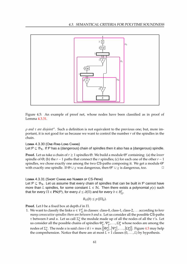
4.3. SEMANTICAL CRITERIA FOR POLYTIME SOUNDNESS
I
Cut
Y
Cut
Y
Y
b
2
2
2
1
1
1
0
0
Π0
Π1
Π2
Figure 4.5: An example of proof net, whose nodes have been classified as in proof ofLemma 4.3.31.
ρ and τ are disjoint”. Such a definition is not equivalent to the previous one; but, more im-portant, it is not good for us because we want to control the number r of the spindles in thechain.
L 4.3.30 (O-R-L C)Let P ⊆ BX. If P has a (dangerous) chain of spindles then it also has a (dangerous) spindle.
Proof. Let us take a chain of r ≥ 1 spindlesΘ. We build a moduleΘ′ containing: (a) the lowerspindle of Θ; (b) the r − 1 paths that connect the r spindles; (c) for each one of the other r − 1spindles, we chose exactly one among the two CS-paths composing it. We get a module Θ′
with exactly one spindle. If Θ ∪ χwas dangerous, then Θ′ ∪ χ is dangerous, too. 2
L 4.3.31 (S C N CS-P)Let P ⊆ BX. Let us assume that every chain of spindles that can be built in P cannot havemore than L spindles, for some constant L ∈ N. Then there exists a polynomial p(x) suchthat for every Π ∈ PN(P), for every d ≤ ∂(Π) and for every b ∈ Bd
Π,
RΠ(b) ≤ p (|Π|d).
Proof. Let b be a fixed box at depth d in Π.1. Wewant to classify the links u ∈ Vd
Πin classes: class-0, class-1, class-2, . . . according to how
many consecutive spindles there are between b and u. Let us consider all the possibleCS-pathsτ between b and u. Let us call Σu
bthe module made up of all the nodes of all the τ’s. Let
us consider all the possible chains of spindles Φub,Ψu
b, . . . ,Ωu
bwhose nodes are among the
nodes of Σub. The node u is said class-i if i = max
∣∣∣Φub
∣∣∣ ,∣∣∣Ψu
b
∣∣∣ , . . . ,∣∣∣Ωu
b
∣∣∣. Figure 4.5 may help
the comprehension. Notice that there are at most L + 1 classes (0, . . . , L) by hypothesis.
61

CHAPTER 4. POLYNOMIALITY IN MS
2. Letmi be the number of Contractions of class-i (they are all at depth d), andm = m0+ . . .+mL.We observe that m ≤ |Π|d.
3. For 0 ≤ i ≤ L, let Πi be the module containing all and only the class- j nodes, for every j ≤ i.4. We define maximal relatively to Πi a CS-path τ starting from b such that there exists a
maximal CS-path τ′ starting from b whose intersection with Πi is exactly τ. So, forexample, the CS-paths maximal relatively to ΠL are exactly the maximal CS-paths in Π.
5. We call Ri, for 0 ≤ i ≤ L, the number of CS-paths starting from b and maximal relativelyto Πi. The definitions imply RΠ(b) = RL.
We prove that Ri ≤∏i
j=0
(m j + 1
)by induction on i. Two CS-paths separate only in a
contraction node, but not in a ⊗L node, which, instead, forces to go in one specific direction.
In Π0 there are no spindles, meaning R0 ≤ m0 + 1. By induction, let Ri−1 ≤∏i−1
j=0
(m j + 1
).
Then, the CS-paths maximal relatively to Πi are at most Ri ≤ Ri−1 · (mi + 1) ≤∏i
j=0
(m j + 1
).
So, RΠ(b) = RL ≤∏L
j=0(mi + 1) ≤ |Π|dL+1. 2
Lemma 4.3.31 and Corollary 4.3.25 directly implies:
P 4.3.32 (S C P)Let P ⊆ BX. Let us assume that every chain of spindles that can be built in P cannot havemore than L spindles, for some constant L ∈N. Then P is strongly polytime.
Some examples. Some useful didactic examples now follow (from Lemma 4.3.33 up toExample 4.3.36). The goal is to begin to understand, given a subsystem P, if it is polytimeor not. The following two Lemmas, in particular, are easy applications of Proposition 4.3.32;but, they can be easily proved also as corollaries of Proposition 4.3.40.
L 4.3.33 (S P S)Let P ⊆ BX, with X = 1, 2, . . . ,M, ordered in the usual way, and whose rules satisfy thefollowing restrictions:
1. if P satisfies Pq(m1, . . . ,mk), then q is greater or equal than every mi, and equal to atmost one among them.
2. if P satisfies Yc(a, b), then c is less or equal than both a and b.
Then P is strongly polytime.
Proof. Let us consider a chain of r spindles. Let us consider two among the ‘main’ rcontractions of the chain. Let us assume the upper one, v, has label Yc(a, b), and the lowerone, u, has label Yd(e, f ). There are two CS-paths starting from u with modalities e, f andarriving in v with modality c. The CS-paths can contain only boxes and contractions: so, byhypothesis, e ≤ c and f ≤ c. But the two CS-paths must join in a box, let us call it B; and atleast one of the CS-paths, by hypothesis, strictly decreases its modality passing through B.We can assume e ≤ c and f < c. Now remember that c ≤ a, b, and we realize that the twolabels must be different: (c, a, b) , (d, e, f ). And this holds for every couple of contractions u, vin the chain: so r ≤ M. We can now apply Lemma 4.3.31 and Proposition 4.3.32 to concludethat the system is strongly polynomial. 2
Similarly:
62

4.3. SEMANTICAL CRITERIA FOR POLYTIME SOUNDNESS
L 4.3.34 (S P S)Let P ⊆ BX, with X = 1, 2, . . . ,M, ordered in the usual way, and whose rules satisfy thefollowing restrictions:
1. if P satisfies Pq(m1, . . . ,mk), then p is greater than every mi.
2. if P satisfies Yc(a, b), then c ≤ a and c < b.
Then P is strongly polytime.
L 4.3.35 (S N-P S)Let P ⊆ BX. Let us assume that: (i) P can build a dangerous chain mA : (Σ ∪ χ) : mA ofspindles (in part. a single dangerous spindle); (ii) mA is a tautology, that is P can prove⊢ mA; (iii) Σ ∪ χ is a proof net; and (iv) P enjoys cut-elimination. Then, P is neither polysize,nor polystep.
Proof. Remember that Σ ∪ χ is a chain of spindles between 2 edges labelled with the samemodality. In this case, moreover the two edges are also labelled with the same formula mA.Using (ii) there exists a closed box b ⊲ ⊢ mA in P. Using b and (iii), we can build the proofnet Θn = Σ 1 . . . 1 Σ︸ ︷︷ ︸
n
1 b. Now, let us try to reduce Θn. In particular, thanks to (iv), we can
decide to reduce the whole level 0, but not the upper levels. In this way, the reduction is notperformed in polysize: the content of b is duplicated 2n times. Now, at level 1 there are aleast 2n new cuts; reducing them, we understand that this reduction is not polystep, too. 2
E 4.3.36 We must be careful in the identification of spindles. Let us consider thefollowing system with 4 modalities:
P =I,⊸R,⊸L,Pm(n, q),Pn(∅),Pq(∅),Pr(n, n, q, q),Ym(n, n),Yn(q, q)
.
If we only look at the rules, we may think P can build a spindle, the more, a dangerousspindle:
Y
Y
m
q
q
n
n
m
However, there is no way to place this spindle inside some proof net. Indeed, by inductionon the construction rules, the reader can check that: (i) for every Π ∈ PN(P) containing therule Pm(n, q) at level 0, there are at most two modal inputs, one with modality n and the other onewith modality q; (ii) for every Π containing the rule Pr(n, n, q, q) there are at most 4 modal inputs,with modality m, n or q; and in particular, (iii) P can only build chains of at most 1 spindle. So thissystem is polytime by Proposition 4.3.32.
63
CHAPTER 4. POLYNOMIALITY IN MS
The system P′ obtained adding e.g. aW rule is not polytime:
P′ =I,⊸R,⊸L,Pm(n, q),Pn(∅),Pq(∅),Pr(n, n, q, q),Ym(n, n),Yn(q, q),W
.
Of course the strange behaviour of P cannot occur in presence of the rules ⊗R or W, nor inpresence of only standard Yi contractions. Indeed the first two rules always allow to createa proof net from a dangerous chain; and the standard contraction is almost useless inside aspindle.
4.3.4 A first Criterion for Polynomial Time Soundness.
The previous results (Proposition 4.3.32, Lemma 4.3.33, and Lemma 4.3.35) give some nec-essary and sufficient conditions for the polynomial time soundness of subsystems. Here,we restrict our attention to sensible subsystems, that have been defined on page 34. In thiscase we improve those theorems coming in particular to Lemma 4.3.39, which simplifiesLemma 4.3.35, and Proposition 4.3.40, that gives a criterion, i.e. a both sufficient and neces-sary condition, for polytime soundness.
We need the following two technical Lemmas.
F 4.3.37 (S P S S)Let P be a sensible subsystem.1. For every l ≥ 0, P contains Πl ⊲A, . . . ,A ⊢ A, with A = γ ⊸ γ, l occurrences of A as
assumptions, and ∂(Πl) = 0.2. Moreover, if h belongs to P, then the formula A can be any one in F X.3. If P proves A, . . . ,A ⊢ A, with l occurrences of A, then it proves also m1A, . . . ,mkA ⊢ qA
for k ≤ l, for every Pq(m1, . . . ,mk) ∈ P.
Proof. Πl is built using one⊸R or h rules, plus l occurrences of the free weakening. 2
L 4.3.38 (B G S)Let P ⊆ BX be a sensible subsystem that can build a (dangerous) spindle Σ. In P there isanother (dangerous) spindle Σ′′ such that: (a) Σ′′ contains only Contractions, Box-out andCut nodes at level 0; (b) Every edge e at level 0 has label qA, for some fixed A; (c) ∂(Σ′′) = 1;and (d) The only premise of Σ′′ is the principal one.
Proof. We begin the proof considering Σ to be a standard, non-dangerous, spindle. The goalis to transform, step by step, Σ into Σ′′.
Let Π ∈ PN(P) be the proof net containing Σ, an example of which is in Figure 4.6a. Wereduce all the linear cuts in Π at level 0. We get to Π′ ∈ PN(P) with Σ′, the reduct of Σ,in it. (See Figure 4.6b.) Σ′ is still a (dangerous) spindle, as well as the residuals of the twoCS-paths ρ, τ of Σ are still CS-paths in Π′. The three CS-paths cannot contain linear nodes.Indeed, we just observe that, e.g., τ must begin in a contraction, with label nA, and muststop in a box, with label mB. So it cannot cross neither any right-node, otherwise it wouldadd a non-modal symbol to nA, and so the last formula could not be mB, nor any left-node,otherwise it would remove a non-modal symbol from nA.
We transform Σ′, just generated, into another graph Σ⋆ by replacing every proof netenclosed in a box Pq(m1, . . . ,mk) of Σ
′ by Πk ⊲A, . . . ,A ⊢ A as in point 1 of Fact 4.3.37 Conse-quently, every qB at level 0 in Σ′ becomes qA in Σ⋆, for some q. This replacement implies∂(Σ⋆) = 1 (Figure 4.6c).
64

4.3. SEMANTICAL CRITERIA FOR POLYTIME SOUNDNESS
Po(m)
⊗R
I I
Pi(m) Pi(n)
⊗L
Cut
⊗R
Po(n)
⊗R
I Po(q)
I I
Pi(q)
Pi(n) Pi(n)
Ym(m,n)
m(B⊗(B⊗qC))
B⊗(B⊗qC)
B B⊗qC
mB n(B⊗qC)
mB⊗n(B⊗qC)
mB
nB
mB
nqC
B⊗qC
B qC
C
(a) Σ
Po(m)
⊗R
I I
Pi(m) Pi(n)
Cut
Po(n)
⊗R
Po(q)
I I
Pi(q)
Pi(n) Pi(n)
Ym(m,n)
m(B⊗(B⊗qC))
B⊗(B⊗qC)
B B⊗qC
n(B⊗qC)
mBnB
mB
nqC
B⊗qC
B qC
C
(b) Σ′
Po(m)
⊸R
W I W
Pi(m) Pi(n)
Cut
Po(n)
⊸R
I
W W
Pi(n) Pi(n)
Ym(m,n)
mA
A
γ
A A
nA
mA nA
mA
mA
A
γ
A A
(c) Σ⋆
Po(m)
⊸R
I
W W
Pi(m) Pi(n)
Cut
Po(n)
⊸R
I
W
Pi(n)
Ym(m,n)
mA
A
γ
A A
nA
mA nA
mA
A
γ
AA
(d) Σ′′
Figure 4.6: Examples relative the proof of Lemma 4.3.38.
Σ⋆ is a graph satisfying the requirements (a)-(b)-(c) in the statement. However in general
65

CHAPTER 4. POLYNOMIALITY IN MS
it does not satisfy (d). Moreover Σ⋆ is not necessarily a spindle, because it may be notcontained in a proof net of P. We can modify Σ⋆ to get a Σ′′ that satisfies the point (d). If eis a non-principal premise of Σ⋆, entering some box b of Σ⋆, then we remove the edge e andwe reduce the number of premises of b, according to point 3 of Fact 4.3.37. Now, we can plugevery non-principal conclusion of Σ′′, exiting upward from some contraction u of Σ′′, with aweakening node: we get a proof netΠ′′ containing Σ′′, thus showing that Σ′′ is a spindle.
At last, if Σ ∪ χwas dangerous, we can apply the same transformation to the CS-path χ,thus arriving to χ′′; Σ′′ ∪ χ′′ is a dangerous spindle. 2
L 4.3.39 (S N-P S S)Let P ⊆ BX be sensible. Let us assume that P can build a dangerous spindle. Then P isneither polysize, nor polystep.
Proof. The proof is similar to the one of Lemma 4.3.35. However, here we have more relaxedhypothesis on Σ. Firstly, we must transform the given dangerous spindle n : (Σ ∪ χ) : n intonA : (Σ′′ ∪ χ′′) :nA, as described in Lemma 4.3.38. Fact 4.3.37 assures the existence of a proofnet b ⊲ ⊢ nA. Now, we call Θn = (Σ′′ ∪ χ′′) 1 . . . 1 (Σ′′ ∪ χ′′)︸ ︷︷ ︸
n
1 b. Remember that we called
exponential chain such an object. Θn is not a proof net because it can have many conclusions,but it can be placed easily inside a proof net Πn closing all its open conclusions with freeweakening nodes. Please notice that |Πn| = O(n). At last, we reduce the first level of Πn.This is possible, thanks to the downward closure of P: the reduction is performed bottom-up,starting from the lower box b. As we already notice when proving Lemma 4.3.35, such areduction is neither polysize, nor polystep. 2
P 4.3.40 (A P C)Let P ⊆ BX sensible, with M modalities. The following are equivalent:1. P is polytime.2. P cannot build any dangerous chain of spindles.3. P cannot build any dangerous spindle.4. P cannot build any chain (neither if not dangerous!) of more than M spindles.
Proof.
4.⇒ 1.We can apply Proposition 4.3.32 with L =M and we get that P is polytime.
¬2. ⇒ ¬1. If P can build a dangerous chain of spindles, Lemma 4.3.39 says that P isneither polystep nor polysize.
¬4. ⇒ ¬2. Let us assume that P can build a chain Θ of r > M spindles. Let w1, . . . ,wr
the principal contractions of the spindles in Θ. By the pigeons-hole principle, at least twoprincipal contractions share the same input label; letwi andw j be the two incriminated nodes,and Σ be the chain of j − i ≤M spindles between them. Σ is dangerous.
3.⇒ 2. Obvious by definition.
2.⇒ 3. This is implied by Lemma 4.3.30. 2
If the system is not sensible, the implication 1. ⇒ 2. may fail; however the implications2.⇔ 3.⇔ 4.⇒ 1. still hold.
66

4.4. SYNTACTICAL CRITERIA FOR POLYTIME SOUNDNESS
C 4.3.41 (P I P)Let P ⊆ BX a polysize sensible system. Then it is also polystep.
Proof. Because if P reduces in polysize, then the same proof of ¬2. ⇒ ¬1. holds: P cannotbuild any dangerous chains of spindles. So, the criterion tells us that, in fact, P is polytime.2
This means, essentially, that no sensible subsystem P of MS can represent PSPACE,unless, of course, PSPACE=PTIME.
We shall apply in Chapter 6 the propositions proved in this Section.
4.3.5 Strong Determinacy
We generalize the definition of “strong determinacy” present in [DL08]. In that work thestrong determinacy of ILAL is used to prove that ILAL is polytime.
D 4.3.42 (S D) A subsystem P ⊆ BX enjoys strong determinacy
iff for every Π ∈ PN(P) and every C ∈ CΠ there is at most 1 context D such that D 7→Π C.
L 4.3.43 (S D P)If P ⊆ BX enjoys strong determinacy, then it is polytime.
Proof. Strong determinacy is equivalent to the absence of spindles in every Π. 2
So, this is a condition sufficient but not necessary for polynomiality.
4.4 Syntactical Criteria for Polytime Soundness
Here, we move towards a different kind of Criteria. We want to avoid the use of contextsemantics, and we would like to understand if a given subsystemP is polytime “just lookingat the building rules it contains”.
4.4.1 Augmented subsystems
Here we will present a class of subsystems that by definition are closed w.r.t. their admissiblerules. Recall that, traditionally, a rule is “admissible” inside a logic if it can be derived insidethat logic, so that it can be freely added to the subsystemwithout changing the set of provablestatements. Here, we will use the term “admissible” in a slightly different way: only someof the derivable rules are admissible, and the admissible rules are really derivable only forsensible subsystems. We shall see that if a subsystem P is polytime, the we can freely addall such admissible rules and we get another polytime system (Proposition 4.4.4). We willcall augmented this larger subsystem. Moreover, we shall see that checking if the augmentedsubsystem is polytime or not is quite easy (Proposition 4.4.5).
D 4.4.1 Given a system P ⊆ BX, we define inductively its admissible (promotion
and contraction) rules.• If P has the rule Pm(m1, . . . ,mk) or Yq(m, n), then it is admissible for P;
67

CHAPTER 4. POLYNOMIALITY IN MS
• If rules Pm(r,m1, . . . ,mk) and Pr(n1, . . . , nl) are admissible for P, so it is the rulePm(n1, . . . , nl,m1, . . . ,mk).• If rulesPm(r,m1, . . . ,mk) andYq(r, s) are admissible forP, then also the rulePm(q,m1, . . . ,mk)is admissible for P.• If rules Pm(m1, . . . ,mk) and Ym(r, s) are admissible for P, then also the rules Pr(m1, . . . ,mk)and Ps(m1, . . . ,mk) are admissible for P.• If rules Ym(r, s) and Yr(q, p) are admissible for P, then also the rules Ym(q, s) and Ym(q, p)are admissible for P.• If rules Ym(r, s) and Pm(q) are admissible for P, then also the rule Yq(r, s) is admissible forP.• If rules Ym(r, s) and Pq(s) are admissible for P, then also the rule Ym(r, q) is admissible forP.
If P is sensible, then all its admissible rules can be derived in P. This can be provedby induction. For example, if P has the two rules Pm(r,m1, . . . ,mk) and Yq(r, s), so thatPm(q,m1, . . . ,mk) is admissible for P, than this latter rule can be proved usingW.
D 4.4.2 (A S S) LetP ⊆ BX. The augmented system
S(P) of P is P plus every admissible rule for P.
If P = S(P) the system is said saturated.
Notice that S(P) contains the closed boxes and it is downward closed. By the definition itfollows that every augmented system S(P) is saturated, i.e. S(S(P)) = S(P). By definition,the augmented system S(P) of P contains one promotion rule for each module of P that canbe built with cuts, contractions and boxes but without spindles.
Every proof net of S(P), in fact, can use rules that are not in P; anyway, if P is sensible,each one of this rules can be decomposed in a number of more primitive rules that are in P:
D 4.4.3 (P P ) Let P ⊆ BX be sensible. Consider a proof net Π inS(P): all the rules of Π can be substituted by a finite number of rules of P; call Π′ the proofnet of P obtained by the rewriting. We call Π′ the primitive proof net of Π.
An example is in Figure 4.7.
P 4.4.4 (P P P S(P))Let us consider a sensible system P ⊆ BX. S(P) ∈ PMS iff P ∈ PMS.
Proof.
⇒) This is just because P ⊆ S(P), and the Monotonicity Lemma 4.1.8 holds.
⇐) If P is polytime, let us assume by contradiction that S(P) is not polytime. Using Propo-sition 4.3.40, we know that S(P) can build a dangerous spindle Σ ∪ χ between twooccurrences of Yq(r, s), while P cannot. However, P and S(P) may differ only for theadmissible rules: Σ contains an admissible promotion or contraction rule of P. But,every admissible rule may be split in a larger number of promotion and contractionrules of P: so the primitive module Σ′ ∪ χ′ of Σ ∪ χ is still a dangerous spindle, and itexists both in S(P) and P. This means that P is not polytime, a contradiction.
68

4.4. SYNTACTICAL CRITERIA FOR POLYTIME SOUNDNESS
o
Po(q)
a
Cut Cut
b c
Pi(m1) Pi(...) Pi(mk)
i i i
o
a
Cut Cut
b c
i i i
Figure 4.7: An example: a possible proof net in an augmented systemS(P), and its primitiveproof net in the original system P.
Y
Y Y
Cut
Y
q
r
s
q
d
u
(a) Σ
Y
q
r s
q
(b) One of the simpler danger-ous spindles induced by Σ.
Figure 4.8: An example of dangerous spindle Σ, as in proof of Proposition 4.4.5.
2
P 4.4.5 (P C B O S)Let P ⊆ BX be a sensible system. Then P is not polytime iff S(P) has the two rules Pq(r, s)and Yq(r, s), for some value of the parameters.
Proof. Using Proposition 4.4.4,P is polytime iff S(P) is polytime. “⇐” case. The presence ofthese two rules leads to a dangerous chain of spindles and soS(P) is not polytime. “⇒” case.If S(P) is not polytime it must have a dangerous spindle Σ ∪ χ between a contraction u and
69

CHAPTER 4. POLYNOMIALITY IN MS
a promotion or contraction d, where the modality s that labels the conclusion of d labels alsothe premise of u. An example is in Figure 4.8. But, thanks to saturated-ness, we can mergeall the nodes and boxes between u and w in a single box, and so we build a new dangerousspindle Σ′ ∪ χ′ made up of only 1 box and 1 contraction, as the thesis requires. 2
4.4.2 Relations among Modalities
Throughout this Section, we consider P ⊆ BX be a fixed subsystem with M < ∞ modalities(for example a sensible subsystem). We define a number of different relations among the Mmodalities. These relations will be used to define some syntactical criteria for the polytimesoundness of P.
The notions of order, preorder and sim. have been recalled in Section 2.10.
D 4.4.6 mR↑ n whenever P can build a CS-path whose edges are all labelled withmodal formulæ, the first one with modality m and the last one with n.
This relation is transitive. It can be built considering all the rules Pn(m) and Ym(n, q), for someq, that can be effectively used in some proof net of P, and then taking the transitive closure.Please recall that it is not obvious that a rule is used inside some proof net of P, unless it issensible (cfr. Fact 3.2.6).
D 4.4.7 mR⋄ nwhenever P can build a spindle m : Σ : n.
This relation is transitive, and it is a sub-relation of R↑. For the moment we neglect thealgorithmic construction of R⋄, even if we think that such algorithm must exist. Howeverthis relation is the most important from a theoretical point of view:
L 4.4.8 (P C B O R⋄)Let P be a sensible subsystem, and R⋄ as before. Then P ∈ PMS iff R⋄ is a strict partialordering.
Proof. We already noticed that R⋄ is transitive. P has a dangerous chain of spindles iff∃n(nR⋄ n), that is if R⋄ is not anti-reflexive. Now, if R⋄ is a partial strict ordering then itis anti-reflexive, so P has no dangerous chains; conversely, if P has no dangerous chains,∀n(¬nR⋄ n), that is R⋄ is anti-reflexive, and thanks to transitivity we conclude also that R⋄ isanti-symmetric, and so a strict partial ordering. 2
We are going to describe a further relation R. Differently from R⋄, R is quite complex,however it is easy to show an algorithm that builds it.
Let P be a sensible subsystem of BX withM < ∞modalities. Let
DM = 〈m〉 | m ∈ X ∪ 〈m, n〉 | m, n ∈ X ;
DM contains the multisets with domain 1, . . . ,M with at least one and most two elements.Letters A,B,C, . . . will temporarily range over elements of DM. |A| ∈ 0, 1 is the cardinalityof A (please notice that |〈m,m〉| = 2 !!!).
By the way, one can show that DM has 12 M(M + 3) elements.
70

4.4. SYNTACTICAL CRITERIA FOR POLYTIME SOUNDNESS
Y I W
u6
u4
u5
u1
u7
u2 u3
Figure 4.9: An example of quasi-connected module, with principal premises u1, u2 andprincipal conclusions u4, u6, u7. Notice that u3 cannot be a principal premise.
D 4.4.9 We define the binary relation R on DM by:
• if P has Pq(m), then 〈m〉R〈q〉 and ∀s〈m, s〉R〈q, s〉;
• if P has Pq(m, n), then 〈m, n〉R 〈q〉;
• ifPhasYq(m, n), then 〈q〉R〈m, n〉, 〈q〉R〈m〉,∀s〈q, s〉R〈m, s〉, 〈q〉R〈n〉, and∀s〈q, s〉R〈n, s〉,
R is the transitive and reflexive closure of R.
R is not, in general, a partial order, even restricting to polytime subsystems.
L 4.4.10P is saturated iff R = R.
Proof. Look back at the definition of R and at the definition of S(P). Their definitions arestep-by-step analogous. So,P is saturated iff its R relation is the greatest possible, i.e. R isclosed. 2
If Σ is a module (not necessarily connected!) of P and A,B ∈ DM, we write A : Σ : Bmeaning that Σ has (at least) |A| premises labelled with modal formulas with modality sfor every element s of A, and (at least) |B| conclusions labelled with modal formulas withmodality s for every element s of B. We call principal premises and principal conclusions
these |A| and |B| edges. We say that Σ is quasi-connected if for every principal premise thereis a CS-path connecting it to a principal conclusion, and for every principal conclusion thereis a CS-path connecting it to a principal premise. In particular every connected module isalso quasi-connected. An example is given in Figure 4.9
L 4.4.11If AR B then there exists a module A : Σ : B quasi-connected.
Proof. If AR B, then either A = B, or (A,B) is in the reflexive closure of R. Firstly, weconsider the case A = B. If A = 〈m〉, the thesis can be proved taking as A : Σ : A the proof netthat contains just one identity node. IfA = 〈m, n〉, the thesis can be proved taking as A : Σ : Athe disconnected module containing two identity nodes, one introducing m and the otherone introducing n. In both cases Σ is quasi-connected.
Now let A , B. In this case (A,B) is in the reflexive closure of R. Being DM a fi-
nite set, AR B implies that we can find a finite number of elements Ai such that A =A0R A1R A2R . . .R Ak = B. We proceed by induction on k.
71

CHAPTER 4. POLYNOMIALITY IN MS
If k = 1, that is AR B, we know that one of the following holds:
1. A = 〈m, n〉R 〈q〉 = B and P has Pq(m, n);2. A = 〈q〉R〈m, n〉 = B iff P has Yq(m, n);3. A = 〈q〉R〈q
′〉 = B and P has Pq′(q) or Yq(q′, s) for some s.
4. A = 〈q, n〉R〈q′, n〉 = B and P has Pq′(q) or Yq(q′, s) for some s.
In each case we can build a module A : Σ : B quasi-connected:
1. one single P has Pq(m, n);2. one single Yq(m, n);3. one among Pq′(q) and Yq(q
′, s).4. two connected components, the first one having one among Pq′(q) and Yq(q
′, s), thesecond one having a single identity node.
If k > 1, let us considerARAk−1R B. By inductive hypothesis there exists aquasi-connectedA : Σ1 : Ak−1. Then, Ak−1 R B tells us there exists a quasi-connected Ak−1 : Σ2 : B, aspreviously showed. Plugging the principal conclusions of Σ1 in the principal premisesof Σ2 we obtain a quasi-connected module A : Σ : B as required.
2
L 4.4.12 (P C B O R)Let P be a sensible subsystem. P has a dangerous chain of spindles iff there exist m, n, q
such that 〈q〉R〈m, n〉R〈q〉.
In other words, if P is polytime, the graph of R may contain cycles; however it cannotcontain cycles with both elements of cardinality 1 and cardinality 2.
Proof. (1) Let us assume P has a dangerous chain Θ∪ χ. Θ∪ χ is composed of a contractionu, let us say Yp(r, s), a box b with 2 premises, and three CS-paths τ, ρ, χ of (possibly many)promotion boxes and contraction nodes, where τ and ρ connect u to b and χ exits from b and
terminates with modality p. By construction, 〈p〉R〈r, s〉R〈p〉.
(2) Let us assume 〈q〉R〈m, n〉R〈q〉. Using Lemma 4.4.11 we can build the quasi-connected modules 〈q〉 : Σ1 : 〈m, n〉 and 〈m, n〉 : Σ2 : 〈q〉. Plugging the principal conclusionsof Σ1 with the principal premises of Σ2 we get a quasi-connected module 〈q〉 : Σ : 〈q〉. Butnotice that, thanks to the definition of quasi-connectedness, Σ is also a dangerous chain ofspindles. 2
C 4.4.13 (P S S D)Let P be a sensible subsystem, and let us assume that the promotion rules of P are de-scribed by means of regular expressions. Then, the question “Is P polytime?” is decidable.
Proof. Notice thatM, the number of modalities in P, is finite, so also the number of possiblepromotion rules “described by means of regular expressions” is finite. So, the algorithm isthe following.1. Make a list of all the rules Yq(m, n), Pq(m) and Pq(m, n) belonging to P. This is possible
because (i) P has M < ∞modalities, and (ii) P is finitely described. So this list is finite.
72

4.4. SYNTACTICAL CRITERIA FOR POLYTIME SOUNDNESS
2. Build the relation R. Each rule found in (i) gives at most a constant number of couplesin R.
3. Build the relation R, the transitive and reflexive closure of R.4. Exhaustively search for q,m, n such that 〈q〉R〈m, n〉R〈q〉.
2
The forthcoming Proposition 4.4.15 is one of our most useful results. It is interesting bothin a theoretical and in an applicative perspective, thanks to the simplicity of the definitionof R↑. The reader can compare Proposition 4.4.15 and Proposition 4.4.5; he will find someanalogies, due to the fact that P and its augmented subsystem S(P) share the same relationR↑. Recall that every transitive relation can be completed to a partial preorder (Section 2.10).
D 4.4.14 R↑ is the smallest partial preorder containing R↑.
In the following statement, ≡ denotes the equivalence under R↑.
P 4.4.15 (C P R↑)Let P ⊆ BX be sensible. P is polytime if and only if, for every 6 elements q1 ≡ q2 ≡ r1 ≡ r2 ≡
s1 ≡ s2, i.e. all equivalent under R↑, P does not contain both Yq1(r1, s1) and Pq2(r2, s2).
Proof. P is not polytime iff P builds a dangerous spindle a : (Σ ∪ χ) : a. By definitions, this isequivalent to say that P has:• a contraction Ya(b, c),• a promotion Pd(e, f ),• a CS-path beginning with modality b and ending with modality e,• a CS-path beginning with modality c and ending with modality f ,• a CS-path beginning with modality d and ending with modality a (this is χ).And this is equivalent to say that P has a contraction Ya(b, c) and a promotion Pd(e, f ) suchthat a ≡ b ≡ c ≡ d ≡ e ≡ f . 2
4.4.3 Maximality in MS
We now consider the following question: is there a notion of largest subsystem of MS whichis polytime? In this Chapter we will show that there is not a single greatest subsystem, buta whole class of maximal subsystems. The word maximal is here used in a technical way,according to algebra and set theory (think to maximal ideals [Vin03], or to maximal elementsof a partial order [DP02]). Here we will define formally what is a maximal subsystem, andwe will give some examples of them. Later, we will prove a Structure Theorem 4.4.25 thatcharacterizes, among the sensible subsystems, all and only the maximal ones. The StructureTheorem is completely syntactical, it describes exactly which rules a maximal subsystemmust have.
The study of maximal subsystems is important for at least two reasons:(a) Themaximal subsystems are useful in themselves, as they supply the greatest sets of rules,
and nevertheless they are polytime. This has impact on the questions that we posed in theIntroduction: if we search for a subsystem able to fill the question mark (3) in Figure 1.2,it is a good idea to begin the search from the maximal subsystems.
73

CHAPTER 4. POLYNOMIALITY IN MS
'
&
$
%
Subsystems of BX
u∅
uBX
u u u u u uu u u u u u uu u u u u u u
u u u u u u
Maximal Polynomial Systems
Polytime subsystems,ILAL included if X ⊇ !, §
Not polytime subsystems,IEAL included if X ⊇ !, §
ILAL
IEAL
Figure 4.10: A picture of the poytime, non-polytime and maximal subsystems of BX.
(b) As we said, the Structure Theorem is completely syntactical; as a corollary, we shall findanother syntactical characterization of the polytime subsystems based on maximality(Proposition 4.4.32).
On the other side, we shall see in Chapter 5 that the maximal subsystems do not have goodcomputational properties. Only few of them enjoy the cut-elimination property; and almostnone of them is confluent. We will recall in Chapter 5 what this means exactly. Here, we justpoint out that the two properties are desirable if we want to use a certain subsystem as aprogramming language, and maximal subsystems do not enjoy them in general. We thinkthat this problem reduces only partially the importance ofmaximal subsystems. The problemaffects the above point (a), but not point (b), so that maximal subsystems are still useful on apractical viewpoint. For example, we can imagine to have a non-maximal subsystem P thatcan be extended in a unique way to a maximal subsystem Q, thus proving that P is polytime,and nevertheless P is confluent. This is the situation, for example, of soLAL (Section 6.2).
D 4.4.16 (M S) A subsystem P ⊆ BX is maximal (for polytime) ifP ∈ PMS, and whenever P ( P′ ⊆ BX, it holds P
′ < PMS.
The picture in Figure 4.10 should help understanding. A weaker notion of maximalityis:
D 4.4.17 (RM S) A subsystemP ⊆ BX of BX is maximal(for polytime) relatively toT ⊆ BX ifP ∈ PMS, andwheneverP ( P′ ⊆ T , it holdsP′ < PMS.
In particular, it is interesting to considermaximality relatively toT = MSY, i.e. the restrictionof MS to standard contractions only.
D 4.4.18 (I) We will call not compatible a rule R w.r.t. a subsystemP if P ∪ R < PMS.
74

4.4. SYNTACTICAL CRITERIA FOR POLYTIME SOUNDNESS
Someexamples. Fordidactic purposes,we are going todescribe somemaximal subsystems.Most of these subsystems contains the linear kernel K, defined on page 29.
L 4.4.19 (T M S)The following subsystems are maximal for polytime:
(a) The subsystem containing every Yp(r, s) for every p, r, s, every P rule, ⊗L,⊸R and all therules introducing ∀, but no W’s, nor ⊗R, nor⊸L.
(b) The subsystem containing K, every Yp(r, s) and every Pr(s) for every p, r, s.The following subsystem is maximal for polytime, relatively to MSY:(c) The subsystem containing K and every P rule, but no contractions.
Proof. We show these subsystems reduce in linear time and they are moreover maximal.
(a) Consider a subsystemwithoutW, ⊗R,⊸L. In this case we can add all the rules we want,including P and Y rules... indeed we will never use them! That’s because there is no wayto have more than one premise in a proof net. The subsystem reduces in linear time. Thissubsystem is maximal: for example, let us try adding W; of course it is not compatiblee.g. with Ym(m,m) and Pm(m,m).
(b) Second case, consider a subsystem made up of all and only rules Pr(s), for all r, s. Here,there is no possible duplication, so we can add every Yp(r, s) and W. This last subsystemis maximal. Indeed, add some rule Pr(s, q); then cut it with Ps(r), Pq(r) and Yr(q, q), andyou have built an exponential chain.
(c) At last, we could have W and all P’s, but no contractions. Also this subsystem triviallyreduces in linear time. This is a maximal subsystem too: if we add Ym, that rule is notcompatible with Pm(m,m). (However note that some other Yp(r, s) could be compatible).
2
L 4.4.20 (O M M S)Let X = 1. The following two subsystems P ⊆ BX are the only maximal subsystemsrelatively to BX:
(a) The subsystem containing Y1, every P rule, ⊗L, ⊸R and the rules introducing ∀, butneither W, nor ⊗R, nor⊸L.
(b) The subsystem containing K, Y1 and P1(1?);
(c) The subsystem containing K and P1(1∗) rules, but no contractions.
Proof. Note that in one-modality subsystems the only possible contraction is Y1, so BX =BX
Y. First, we show these subsystems are maximal:
(a),(b) Analogous to Lemma 4.4.19 (a) and (b).(c) There is no way of getting a spindle, so this is polytime. Of course we cannot add Y1(1, 1)
because it’s not compatible with P1(1, 1).Now, the point is, are there some more maximal subsystems? We prove there are not. If Pis maximal and does not contain Y1, it must be (c). If P is maximal and contains Y1, it cancontain P1(1
∗) (so it must be (b)) or it doesn’t (so it must be (a)).
What about ∀,⊗,⊸? Except for the trivial case (a), they are not dangerous, and so theyare needed in every maximal subsystem. 2
75

CHAPTER 4. POLYNOMIALITY IN MS
Basic properties of maximal subsystems. From now on, we will consider sensible andmaximal subsystems. Our main result is the Structure Theorem 4.4.25. In order to prove it, we
shall study the relations R↑, R,R among the modalities, that were defined in Section 4.4.2.We are interested in particular to understand whether these relations are linear or partialorders or preorders. The definitions of linear/partial (pre-)orders were given in Section 2.10.
In this paragraphwegive somebasicproperties about the relationsR↑,R,R; theywill berequired to prove the Structure Theorem. We give also some other, unrelated, properties. Inparticular, Lemma 4.4.21 reveals the relationship betweenmaximal subsystems and saturatedsubsystems, that were studied in Section 4.4.1, and Corollary 4.4.23 shows that the question:“is P maximal?” is in most cases decidable.
L 4.4.21 (M . S S)All the sensible maximal subsystems are saturated.
Proof. By contradiction, let P be maximal but not saturated. Then, S(P) would be polytimefor Lemma 4.4.4; and so P would not be maximal, a contradiction. 2
However the converse is false; for example, a sensible subsystem with all and only theclosed boxes, and without contractions, is trivially saturated, but it is not maximal.
L 4.4.22 (R M S M C)Let P be a sensible maximal subsystem.1. If P has Pq(
−→m, n, n) it also has Pq(
−→m, n∗).
2. If P has Pq(m, n) and Pq(n, r) it also has Pq(m, n, r).3. ∀q ∈ X, P has at least Pq(q?). That is, R↑ is reflexive.4. R = R.
Proof. The justification to the first point develops as follows. Sensibility is needed byProposition 4.3.40. P cannot have Pq(
−→m, n∗) if such a rule generates a spindle. In that case,
the same spindle exists thanks to Pq(−→m, n, n) against the maximality of P. An analogous
argument can be used to justify the second point. The third one is obvious because Pq(q?)
has at most an assumption. 2
C 4.4.23 (M D)Let P be a sensible subsystem, and let us assume that the promotion rules of P are de-scribed by means of regular expressions. Then, the problem “Is P maximal w.r.t. polynomialtime?” is decidable.
Proof. We present a very naıve algorithm that solves the problem. Notice that P hasM < ∞modalities, so the possible rules Yq(n,m), Pq(m) and Pq(m, n) are finite. So, (1) for each suchrule R, check if the subsystemP∪R is polytime. This is possible thanks to Lemma 4.4.13. Ifso, we are sure that P is not maximal. Otherwise, (2) we must check that the rules describedby Fact 4.4.22 are in P. No other rules can be considered, so the subsystem is maximal iff theanswer to (2) is positive. 2
76

4.4. SYNTACTICAL CRITERIA FOR POLYTIME SOUNDNESS
L 4.4.24 (R↑ L P)Let P be a sensible maximal subsystem. Then R↑ is linear preorder, i.e. transitive, reflexiveand connected.
Proof. R↑ is always transitive. Here it is also reflexive, because of the presence of Pq(q). Wehave to prove that it is connected, that is: ∀m, n (mR↑ n ∨ nR↑m). Let us assume that P
is maximal and ¬(mR↑ n
); we will show that nR↑m. This implies that adding Pn(m) to P
gives a non-polytime subsystem P′. So we can find a dangerous spindle q : (Σ ∪ χ) : q in P′
containing Pn(m). This spindle is not in P, however in P we can find a module Σ′ ∪ χ′ suchthat, adding a correct number of instances of Pn(m) boxes, gives Σ. In particular we find inΣ′ (and so in P) two paths, one from modality q to m and the other one from n to q, that canbe composed to create a path from n to m: so nR↑m. 2
So, from now on, we shall write also in place of R↑, ≺ for the corresponding strictpreorder, and m ≡ nwhenever both m n and n m.
Differently fromR↑,R is not a preorder; in general it is not even connected. For example,consider X = 1, 2, 3, 4, 5,
P = P4(3, 4),Y4(1, 4),P5(5, 1),Y5(5, 2).
P is polytime because R↑ is a linear order:
3 ≺ 4 ≺ 1 ≺ 5 ≺ 2
and satisfies the hypothesis of Lemma 4.3.33. But it is not maximal: it can be embedded insome othermaximal subsystemP′. We are not interested in the exact form ofP′; we justwantto observe that P′ cannot have neither the rule Y1(2, 3), nor P1(2, 3), because both of them
permit the constructionof somedangerous chain. So both¬(〈1〉R〈2, 3〉
)and¬
(〈2, 3〉R〈1〉
).
That is, R is not connected.So, it turns out that the relation has a great importance in the study ofmaximal systems,
and we shall use it (instead of R, or other) in proving the Structure Theorem.
Structure Theorem for Maximal Subsystems. We are going to restrict our attention to thesubsystem in which is a linear order (i.e. a connected partial order, see Section 2.10). Later,we shall see that this assumption is fully justified, i.e. maximal subsystems whose is alinear order are more interesting that the other ones.
T 4.4.25 (S M S S)Let P be a sensible subsystem with a linear and with modalities in X. P is maximal iff Pcontains exactly the following rules:1. all the rules Yq(m, n) for every choice of q ≺ m, n in X;2. all the rules Yq(q, n) for every choice of q ≺ n in X;3. all the rules Pq(q
?,m∗1, . . . ,m∗
k) for every choice of m1, . . . ,mk ≺ q in X;
4. only one among Yq(q, q) and Pq(q∗,m∗
1, . . . ,m∗
k), for every m1 . . . ,mk ≺ q in X.
Proof. “Only if” direction. We want to prove that every system P containing the rulesdescribed in points 1, 2, 3, 4 is maximal. The order prevents to construct dangerousspindles thanks to its linearity. So, Proposition 4.3.40 implies P is polytime. Moreover, if
77
CHAPTER 4. POLYNOMIALITY IN MS
Yq(q, q) belongs to P, adding Pq(q∗,m∗
1, . . . ,m∗
k), against point 4, would allow to construct a
dangerous spindle. The same would be by starting with Pq(q∗,m∗
1, . . . ,m∗
k) in P and, then,
adding Yq(q, q).“If” direction. We assume P is maximal and we want show that it must contain at least
all the rules described in the statement. We prove it by contradiction first relatively to points1, 2, and 3, then to point 4. A contradiction relative to points 1, 2, and 3 requires to assumethat P has not a rule R described in 1, 2, 3. Let P′ = P ∪ R. The maximality of P impliesthat P′ is not polytime. Now, thanks to Proposition 4.3.40, P′ < PMS implies that P′ canbuild a dangerous spindle r : (Σ ∪ χ) : r. We are going to see that this causes various kinds ofcontradictions.
Let u be an instance of R = Yq(m, n). For example, we can assume that one of the twodistinct CS-paths in Σ crosses u from qA to mA. By definition of , r q ≺ m r, socontradicting the linearity of .
Let u be an instance ofR = Yq(q, n). The previous case excludes that one of the two distinctCS-paths in Σ crosses u from qA to nA. So, it must cross u from its premise, labeled qA to itsconclusion, labeled qA. This means that r :Σ′ ∪ χ′ : r, obtained from Σ ∪ χ just removing u,exists in P, which could not be polytime.
The case R = Pq(q,m1, . . . ,mk) combines the two previous ones.Now we move to prove point 4. Without loss of generality, we can prove the thesis for
Pq(q, q) instead of Pq(q∗,m∗
1, . . . ,m∗
k). By contradiction, let P be maximal and let the thesis be
false. So, there are R1 = Yq(q, q) and R2 = Pq(q, q) such that eitherP has both of them, orP hasnone of them. In the first case the two rules would build a spindle, making P not polytime.In the second case, neither R1 nor R2 belong to P. This means that neither P1 = P ∪ R1,nor P2 = P ∪ R2 are polytime, because, recall, P is maximal. So, there have to exist bothr1 : (Σ1∪χ1) : r1 inP1 that involves an instance u1 of R1 (Figure 4.11a), and r2 : (Σ2∪χ2) : r2 inP2
involving the instance b2 of R2 (Figure 4.11b). Thanks to Lemma 4.3.38 we can assume thatall the labels in Σ1 ∪ χ1 and Σ2 ∪ χ2 are of the form nA, for a fixed A and some n’s. Then, u1must be the principal contraction of Σ1. If not, we could eliminate it as we did for u in point2, proving that P is not polytime. This is why r1 = q in Σ1 ∪ χ1 of Figure 4.11a. Now, let Θbe the module obtained from Σ1 ∪χ1 removing u1; we can build Θ in P (Figure 4.11c). Θ hastwo premises qA and one conclusion qA, exactly as the box b2 in Σ2. So, we can replace b2 inΣ2 ∪ χ2 with Θ, getting a new dangerous spindle r2 : (Σ ∪ χ) : r2 in P. But (Σ ∪ χ) ∈ PN(P), sothat P is not polytime. 2
Thanks to the Structure Theorem, we can count the maximal subsystems:
C 4.4.26 (N M S)Let #X = M. There are 2M maximal and sensible subsystems of BX, whose relation is alinear order.
Proof. 2M because, for each of the M modalities, one has to choose among the rule Pi(i∗) or
Yi. 2
It follows an observation about the spindles relation R⋄, defined in Section 4.4.2:
C 4.4.27 (R⋄ ≺)Let P be a maximal sensible subsystem whose R↑ (or ) relation is a linear order. Then itsR⋄ is a strict linear order, and so it is equal to ≺.
78

4.4. SYNTACTICAL CRITERIA FOR POLYTIME SOUNDNESS
Yq(q,q)
r1A=qA
u1
qAqA
r1A=qA
(a) r1 : (Σ1 ∪ χ1) :r1 in P1
Pq(q,q)
Y
r2A
b2
qA
qAqA
u2
r2A
(b) r2 : (Σ2∪χ2) :r2 inP2
qA
qA qA
(c) Θ from Σ1
Θ
Y
r2A
qA
qAqA
r2A
(d) r2 : (Σ ∪ χ) :r2 in P
Figure 4.11: The proof nets used in the proof of Theorem 4.4.25
Proof. Thanks to Structure Theorem, for every m ≺ n we can build a spindle using Ym(m, n)and Pn(m, n), and so mR⋄ n. 2
If R↑ is not an order, the Corollary 4.4.27 may fail. Consider for example X = 1, 2, 3,
P = P1(1?),P2(1
∗, 2∗, 3∗),P3(1∗, 2∗, 3∗),Y1(x, y) for x, y ≤ 3.
This is maximal, 1R⋄ 2, 1R⋄ 3, but 2 and 3 incomparable.
What if is not an Order. We shall see that this case can be brought back to the previousone. If is a linear preorder overX, then it naturally induces a linear order over the quotientX′ = X /≡, where m ≡ n iff m n and n m (cfr. Section 2.10). m denotes the equivalenceclass of m.
D 4.4.28 (N Q P) LetP ⊆ BX sensible. Recall that is a preorder,and letX′ the quotient ofX as just described. Let P′ ⊆ BX′ be the smallest subsystem ofBX′
such that:
Pq(−→m)∈ P ⇒ Pq
(−→m
)∈ P′,
Yq(m, n) ∈ P ⇒ Yq(m, n)∈ P′.
P′ is called natural quotient of P.
F 4.4.29For every P, the relation of P′ is a linear order.
The Fact directly follows from the construction.
L 4.4.30 (L O I)Let P ⊆ BX sensible, and P′ ⊆ BX′ be its natural quotient. Then, P is polytime iff P′ ispolytime.
Proof. “⇒”. If P can build a dangerous chain of spindles, then by construction P′ can buildthe same chain, too.
79
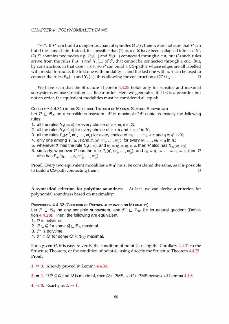
CHAPTER 4. POLYNOMIALITY IN MS
“⇐”. If P′ can build a dangerous chain of spindlesΘ∪χ, then we are not sure that P canbuild the same chain. Indeed, it is possible that (1)m, n ∈ X have been collapsed intom ∈ X′,(2) Σ′ contains two nodes e.g. Pm(...) and Ym(...) connected through a cut, but (3) such rulesarrive from the rules Pm(...) and Yn(...) of P, that cannot be connected through a cut. But,by construction, in that case m n, so P can build a CS-path τ whose edges are all labelledwith modal formulæ, the first one with modality m and the last one with n. τ can be used toconnect the rules Pm(...) and Yn(...), thus allowing the construction of Σ′ ∪ χ′. 2
We have seen that the Structure Theorem 4.4.25 holds only for sensible and maximalsubsystems whose relation is a linear order. Here we generalize it. If is a preorder, butnot an order, the equivalent modalities must be considered all equal:
C 4.4.31 ( S T M S S)Let P ⊆ BX be a sensible subsystem. P is maximal iff P contains exactly the followingrules:1. all the rules Yq(m, n) for every choice of q ≺ m, n in X;2. all the rules Yq(q
′, n) for every choice of q ≺ n and q ≡ q′ in X;3. all the rules Pq(q
′?,m∗1, . . . ,m∗
k) for every choice of m1, . . . ,mk ≺ q and q ≡ q′ in X;
4. only one among Yq(q, q) and Pq(q∗,m∗
1, . . . ,m∗
k), for every m1 . . . ,mk ≺ q in X;
5. whenever P has the rule Yq(q, q), and q1 ≡ q2 ≡ q3 ≡ q, then P also has Yq1(q2, q3).6. similarly, whenever P has the rule Pq(q
∗,m∗1, . . . ,m∗
k), and q0 ≡ q1 ≡ . . . ≡ qt ≡ q, then P
also has Pq0(q1, . . . , qt,m∗1, . . . ,m∗
k).
Proof. Every two equivalent modalities q ≡ q′ must be considered the same, as it is possibleto build a CS-path connecting them. 2
A syntactical criterion for polytime soundness. At last, we can derive a criterion forpolynomial soundness based on maximality:
P 4.4.32 (C P M)Let P ⊆ BX be any sensible subsystem, and P′ ⊆ BX′ be its natural quotient (Defini-tion 4.4.28). Then, the following are equivalent:1. P is polytime.2. P ⊆ Q for some Q ⊆ BX maximal.3. P′ is polytime.4. P′ ⊆ Q′ for some Q′ ⊆ BX′ maximal.
For a given P, it is easy to verify the condition of point 2., using the Corollary 4.4.31 to theStructure Theorem, or the condition of point 4., using directly the Structure Theorem 4.4.25.
Proof.
1.⇔ 3. Already proved in Lemma 4.4.30.
2.⇒ 1. If P ⊆ Q and Q is maximal, then Q ∈ PMS, so P ∈ PMS because of Lemma 4.1.8.
4.⇒ 3. Exactly as 2.⇒ 1.
80
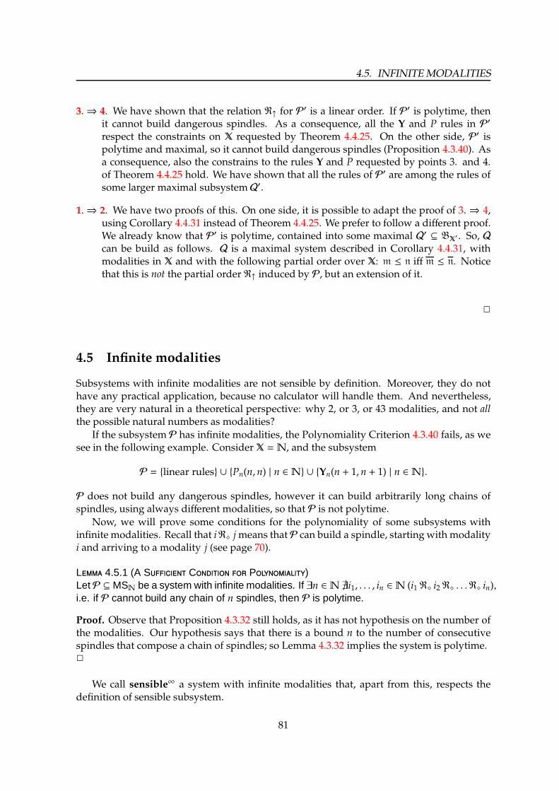
4.5. INFINITEMODALITIES
3.⇒ 4. We have shown that the relation R↑ for P′ is a linear order. If P′ is polytime, then
it cannot build dangerous spindles. As a consequence, all the Y and P rules in P′
respect the constraints on X requested by Theorem 4.4.25. On the other side, P′ ispolytime and maximal, so it cannot build dangerous spindles (Proposition 4.3.40). Asa consequence, also the constrains to the rules Y and P requested by points 3. and 4.of Theorem 4.4.25 hold. We have shown that all the rules of P′ are among the rules ofsome larger maximal subsystemQ′.
1.⇒ 2. We have two proofs of this. On one side, it is possible to adapt the proof of 3. ⇒ 4,using Corollary 4.4.31 instead of Theorem 4.4.25. We prefer to follow a different proof.We already know that P′ is polytime, contained into some maximal Q′ ⊆ BX′ . So, Qcan be build as follows. Q is a maximal system described in Corollary 4.4.31, withmodalities in X and with the following partial order over X: m ≤ n iff m ≤ n. Noticethat this is not the partial order R↑ induced by P, but an extension of it.
2
4.5 Infinite modalities
Subsystems with infinite modalities are not sensible by definition. Moreover, they do nothave any practical application, because no calculator will handle them. And nevertheless,they are very natural in a theoretical perspective: why 2, or 3, or 43 modalities, and not allthe possible natural numbers as modalities?
If the subsystem P has infinite modalities, the Polynomiality Criterion 4.3.40 fails, as wesee in the following example. ConsiderX =N, and the subsystem
P = linear rules ∪ Pn(n, n) | n ∈N ∪ Yn(n + 1, n + 1) | n ∈N.
P does not build any dangerous spindles, however it can build arbitrarily long chains ofspindles, using always different modalities, so that P is not polytime.
Now, we will prove some conditions for the polynomiality of some subsystems withinfinite modalities. Recall that iR⋄ jmeans thatP can build a spindle, starting with modalityi and arriving to a modality j (see page 70).
L 4.5.1 (A S C P)LetP ⊆ MSN be a system with infinite modalities. If ∃n ∈N∄i1, . . . , in ∈N (i1R⋄ i2R⋄ . . .R⋄ in),i.e. if P cannot build any chain of n spindles, then P is polytime.
Proof. Observe that Proposition 4.3.32 still holds, as it has not hypothesis on the number ofthe modalities. Our hypothesis says that there is a bound n to the number of consecutivespindles that compose a chain of spindles; so Lemma 4.3.32 implies the system is polytime.2
We call sensible∞ a system with infinite modalities that, apart from this, respects thedefinition of sensible subsystem.
81

CHAPTER 4. POLYNOMIALITY IN MS
L 4.5.2 (A S C N-P)Let P be a sensible∞ system. If ∀n ∈ N ∃i1, . . . , in ∈ N (i1R⋄ i2R⋄ . . .R⋄ in), i.e. if P canbuild chains of spindles i1 :Θn : in arbitrarily long, and moreover the size of these chains is|Θn| = O(n), then P is not polytime.
Proof. For every n we find a chain of n spindles. This chain can be chosen with size O(n) byhypothesis, and depth 1, thanks to Lemma 4.3.38. So, following the proofs of Lemma 4.3.35and 4.3.39, we understand that P is not polytime. 2
We can see that there is a third, possible case, not contemplated by the two previousLemmas. This is the case in which P can build chains of spindles arbitrarily long, buthowever their size is very big, e.g. O (2n). In this case, actually we don’t know if P ispolytime or not. If P is saturated and sensible∞, the previous Lemmas can be extended inorder to include all the three cases:
C 4.5.3 (A P C S S)Let P be a subsystem sensible∞ and saturated. Then P is polytime if and only if ∃n ∈N ∄i1, . . . , in ∈N (i1R⋄ i2R⋄ . . .R⋄ in).
Proof. “⇐”. If∃n ∈N∄i1, . . . , in ∈N (i1R⋄ i2R⋄ . . .R⋄ in), thenP is polytime for Lemma4.5.1.“⇒”. Let ∀n ∈ N ∃i1, . . . , in ∈ N (i1R⋄ i2R⋄ . . .R⋄ in). This means that, for every n, a chainof spindles Θn can be built. Notice that, whenever m : Σ : n is a spindle, the hypothesis ofsaturation let us to create another spindle m : Σ′ : n with just one box and one contraction.As a consequence, fromΘn it is possible to build another chain of spindlesΘ′n with sizeO(n).Lemma 4.5.2 can now be applied. 2
Corollary 4.5.3 highlights the difference between sensible and sensible∞ subsystems. Forsensible∞ subsystems, Proposition 4.4.4 fails: it is possible that a sensible∞ subsystem P ispolytime, while its augmented system is not.
A different (but similar) kind of polynomiality can be proved, in analogy to Lemma 8.1.5:
L 4.5.4 (A S C W P)Let P ⊆ MSX be a system with infinite modalities. Let us suppose that P cannot builddangerous spindles. Let us suppose moreover that (i) there is a linear ordering among themodalities of X, (ii) this linear order is a well-ordering with order type at most ω, and (iii) therules of P respect this ordering. Then, there exists a family of polynomials p∂,M(x) | ∂,M ∈N such that for everyΠ ∈ PN(P) with depth at most ∂ and whose modalities have order-typeat most M, [Π] and ‖Π‖ are bounded by p∂,M(|Π|).
Proof. The long hypothesis about the well-ordering is needed to obtain that, wheneverΠ →∗ Σ, then also the modalities of Σ have order-type at most M. Now, if P is a subsystemthat uses only the first M modalities of the ordering of X, we apply Proposition 4.3.40 andwe find that P is polytime. Finally, we put the obtained polynomials all together. 2
82

Chapter 5
Computational Properties in MS
In this Chapter we will face two properties that, traditionally, are considered indefeasible inlight logics: cut-elimination and confluence. A logic enjoys the cut-elimination property if everycut inside a proof can always be reduced. A logic enjoys confluence (or: it is Church-Rosser)if whenever a proof can reduce in two different ways, then the two reducts may still reduceto a common form. Such two properties are not guaranteed for subsystems of MS.
In Section 5.1 we shall characterize, among the maximal subsystems, those ones enjoyingthe cut-elimination property. In Section 5.2 wewill see that almost everymaximal subsystemis not confluent. We shall also see some properties that force a subsystem to be confluent. Forexample, the subsystems that have cut-elimination and that use only standard contractions(i.e. of kind Ym(m,m)) are also confluent (Lemma 5.2.6).
5.1 About Cut-elimination
F 5.1.1 (C E L K)Let P ⊆ BX. All the linear cuts can always be eliminated. If P contains the linear kernel, alsothe gc cuts can be eliminated.
Proof. The linear cuts annihilate, without any need of new nodes. The gc cuts may createnew nodes, but all these are among the nodes of the linear kernel. 2
F 5.1.2 (C E S S)Let P ⊆ BX be saturated. Then, every [P/P] cut can be reduced.
Proof. By definition of saturation. 2
F 5.1.3 (C E S S)Let P ⊆ BX sensible. Every cut involving a closed box is reducible.
Proof. The definition of sensible subsystem requires both the presence of all the closed boxesand the downward closure. 2
83

CHAPTER 5. COMPUTATIONAL PROPERTIES IN MS
P 5.1.4 (C S M S C-E)Let us consider P ⊆ MS sensible and maximal w.r.t. polytime soundness, such that its R↑relation is a linear order. Then, P enjoys cut elimination iff it exists q ∈ X such that(i) for all the modalities m, with m q, P has Ym, and so not Pm(m∗);(ii) for all the modalities m, with q ≺ m, P has Pm(m
∗), and so not Ym.
Proof. Let us assume there exists such q; we want to prove that P enjoys cut-elimination.The only problematic ns are [P/P] and [P/Y]. If a box Pm(n1, . . . , nk, r) is cut with a boxPr(s1, . . . , sl), the linear order says that ∀i, j, si r and n j, r m. The cut must reduce toPm(~n,~q). There are three cases. (1) If at most one among the ni’s and s j’s is m, then the rulePm(~n,~q) is in P for maximality. (2) If 2 or more among the ni’s are m, then the P has therule Pm(m
∗) by maximality, and so it has also Pm(~n,~s). (3) If 2 or more among the ni’s ands j’s are m, and at least one among the s j’s is m, then r = m and one of the boxes is in factPm(m,m, . . .); again, for maximality P must have the rule Pm(~n,~s). So, let us consider a cutbetween a contraction and a box. There are several different cases. (1) If the box is closed,the reduction can be performed for downward closure. (2) Ys(m, n), with s ≺ m and s n, iscut with Ps(r1, . . . , rk, t) with ri ≺ s and t s. This can be reduced by maximality, using rulesPm(s, . . . , s,m), Pn(r1, . . . , rk, s), Yri(s, ri) and Yt(m, s). (3) Ys(s, s) is cut with Ps(r1, . . . , rk, t) withri ≺ s and t s. Of course s q, so we can reduce it using rules Ps(r1, . . . , rk, t), Y
ri and Yt. (4)Symmetric: Ys(m, n), with s ≺ m and s n, is cut with Ps(r1, . . . , rk, s
∗) with ri ≺ s. Now q ≺ s,so we can reduce the cut using rules Pm(m
∗), Pn(n∗, s∗), Yri(m, n), Ys(m, s).
Conversely, let us assume that P does not satisfy this condition. We can find m, n, wherem ≺ n and ∄r(m ≺ r ≺ n), such that P has the rules Pm(m
∗) and Yn. As an example, the readercan try to reduce a cut between Yn and Pn(m,m); it is not possible. 2
The following improves Corollary 4.4.26:
C 5.1.5 (N M S C-)Let #X = M. There are M maximal and sensible subsystems of BX, whose relation is alinear order and that satisfy cut-elimination.
Proof. M because q of Proposition 5.1.4 can be chosen in justM ways. 2
5.2 About Confluence
Intuitively, a rewriting system is confluent whenever each computation leads to a uniqueresult. This has been formally stated in Section 3.4.1, where we have recalled moreover thatdifferent kinds of confluence (called CR, WCR, UN) exist for ARS. In a first moment, whenour aim was just to study polynomial soundness of our subsystems, confluence was not anissue. But, when we are interested also to programming inside a subsystem P, confluencebecomes a useful property: each program comes to a unique result. In this Section we willprovide some condition that allows a subsystem to be confluent (Corollary 5.2.2); but, moreimportantly, we show thatmost of themaximal sensible subsystems are notCR (Lemma5.2.4).
We rephrase the properties CR, WCR, UN in terms of proof nets. In that way, we willnever need to refer to ARS.
84

5.2. ABOUT CONFLUENCE
• A subsystemP is WCR if, wheneverΠ,Σ1,Σ2 ∈ PN(P), Π→ Σ1 andΠ→ Σ2, there existsΘ ∈ PN(P) such that Σ1 →
∗ Θ and Σ2 →∗ Θ.
• A subsystem P is CR if, wheneverΠ,Σ1,Σ2 ∈ PN(P), Π→∗ Σ1 and Π→∗ Σ2, there exists
Θ ∈ PN(P) such that Σ1 →∗ Θ and Σ2 →
∗ Θ.• Let ≡ denotes the smallest equivalence relation containing→∗. A subsystem P is UN if,wheneverΠ,Σ ∈ PN(P) are normal forms, and Π ≡ Σ, thenΠ = Σ.
Recall that WCR is equivalent to CR (cfr. Corollary 3.4.3), and they both imply UN.
The following is a first, naıve, result:
L 5.2.1 (C S)Let P ⊆ BX sensible. P is CR iff it satisfies all the following conditions:
1. If P has rules Yq(m, n) and Pq(r,~s) and the cut of these two rules is reducible, then thereis only one way to reduce it.
2. If P has rules Yq(m, n), Pq(p,~r), Pp(~s), and both cuts among the rules are reducible, thenthere exists a common normal form for Yq(m, n) 1 Pq(p,~r) 1 Pp(~s) in 1 step.
3. If P has rules Pm(n,~r), Pn(p,~s), Pp(~q), and both cuts among the rules are reducible, thenthere exists a common normal form for Pm(n,~r) 1 Pn(p,~s) 1 Pp(~q) in 1 step.
4. If P has rules Pm(n, p,~r), Pn(~s), Pp(~q), and both cuts among the rules are reducible, thenthere exists a common normal form for Pn(~s) 1 Pm(n, p,~r) 1 Pp(~q) in 1 step.
Proof. If P does not satisfy these conditions, than it is easy to build some non-confluentproof nets. For 3. and 4. use the two suggested proof nets: resp. Pm(n,~r) 1 Pn(p,~s) 1 Pp(~q)and Pn(~s) 1 Pm(n, p,~r) 1 Pp(~q). For 1. and 2. the proceeding is similar, but it is necessary atleast a pair of identities and a tensor right in order to close the two dangling conclusions of thecontraction. Sensibility gives the required node.
Conversely, let us assume P has the given properties. Thanks to Corollary 3.4.3, we justneed to check the subsystem isWCR. Let us fix proof netsΣ1 ← Π→ Σ2 in PN(BX), obtainedeliminating two different cuts c, c′. If c, c′ do not affect each other, we just apply both themand we obtain a common normal form Θ. Otherwise, the only problematic cases involve[P/P] and [Y/P] ns; thanks to the 4 hypothesis, P has rules enough to obtain the desiredcommon result Θ. 2
The same Lemma 5.2.1 can be rewritten in Corollary 5.2.2 in amore computational fashion.Suchanewcorollary is quite ugly, butwe shall see that it implies the importantCorollary 5.2.3.
C 5.2.2 (C S)Let P ⊆ BX sensible. P is CR iff it satisfies all the following conditions:
1. If P has rules Yq(m, n) and Pq(r,~s) and the cut of these two rules is reducible, then thereis only one way to reduce it.
2. If P has rules Yq(m, n), Pq(p,~r), Pp(~s), Pm(a, ~u), Pn(b, ~v), Yp(a, b), Yrα(uα, vα) for everyα (where ~u = 〈u0 . . .uA〉), and Pq(~r,~s), then P has also, for some ~w,~z: Pa(~w), Pb(~z),Ysβ(wβ, zβ) for every β (where ~s = 〈s0 . . . sB〉), and Pm(~w, ~u), Pn(~z, ~v).
85

CHAPTER 5. COMPUTATIONAL PROPERTIES IN MS
3. If P has rules Pm(n,~r), Pn(p,~s), Pp(~q), Pm(p,~r,~s), Pn(~q,~s), then it has also the rulePm(~r,~s,~q).
4. If P has rules Pm(n, p,~r), Pn(~s), Pp(~q), Pm(p,~r,~s), Pm(n,~r,~q), then it has also the rulePm(~r,~s,~q).
If P is saturated (and so in particular if it is maximal), then the two first conditions are enough.
Proof. The first part of the statement is a trivial consequence of Lemma 5.2.1. For the laststatement, observe that the last two conditions are satisfied thanks to saturation. 2
C 5.2.3 (C D)Let P be a sensible subsystem, and let us assume that the promotion rules of P are de-scribed by means of regular expressions. Then, the problem “Is P CR?” is decidable.
However, in most of the cases the hypothesis of Corollary 5.2.2 cannot be satisfied, as thefollowing, gloomy, Lemma shows:
L 5.2.4 (M S CR)Let X have at least three elements, P ⊆ BX be sensible and maximal, whose relation is alinear order. Then, P is not CR.
Proof. Let r, q,m ∈ X three different modalities such that r ≺ q ≺ m. We consider thefollowing proof net of PN(P) (it exists by maximality):
⊗R
I I
Yq(m,m)
Cut
Pq(r)
m m
q
r
This cut is reducible in at least two different ways (again, they both exist by maximality):
⊗R
I I
Cut Cut
Pm(m) Pm(m)
Yr(m,m)
m m
m m
r
⊗R
I I
Cut Cut
Pm(q) Pm(q)
Yr(q,q)
m m
q q
r
At this point, we can still eliminate the [I/ ] cuts, and we reach two different normal forms.2
86
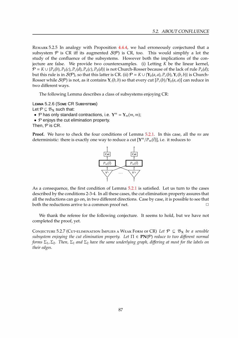
5.2. ABOUT CONFLUENCE
R 5.2.5 In analogy with Proposition 4.4.4, we had erroneously conjectured that asubsystem P is CR iff its augmented S(P) is CR, too. This would simplify a lot thestudy of the confluence of the subsystems. However both the implications of the con-jecture are false. We provide two counterexamples. (i) Letting K be the linear kernel,P = K ∪ Pa(b),Pb(c),Pc(d),Pa(c),Pb(d) is not Church-Rosser because of the lack of rule Pa(d);but this rule is in S(P), so that this latter is CR. (ii) P = K ∪ Yb(a, a),Pc(b),Yc(b, b) is Church-Rosser while S(P) is not, as it contains Yc(b, b) so that every cut [Pc(b)/Yb(a, a)] can reduce intwo different ways.
The following Lemma describes a class of subsystems enjoying CR:
L 5.2.6 (S CR S)Let P ⊆ BX such that:• P has only standard contractions, i.e. Ym = Ym(m,m);• P enjoys the cut elimination property.
Then, P is CR.
Proof. We have to check the four conditions of Lemma 5.2.1. In this case, all the ns aredeterministic: there is exactly one way to reduce a cut [Ym/Pm(~r)], i.e. it reduces to
Cut Cut
Pm(~r) Pm(~r)
Yr1 . . . YrA
As a consequence, the first condition of Lemma 5.2.1 is satisfied. Let us turn to the casesdescribed by the conditions 2-3-4. In all these cases, the cut elimination property assures thatall the reductions can go on, in two different directions. Case by case, it is possible to see thatboth the reductions arrive to a common proof net. 2
We thank the referee for the following conjecture. It seems to hold, but we have notcompleted the proof, yet.
C 5.2.7 (C- I W F CR) Let P ⊆ BX be a sensiblesubsystem enjoying the cut elimination property. Let Π ∈ PN(P) reduce to two different normalforms Σ1,Σ2. Then, Σ1 and Σ2 have the same underlying graph, differing at most for the labels ontheir edges.
87

CHAPTER 5. COMPUTATIONAL PROPERTIES IN MS
88

Chapter 6
Interesting Subsystems of MS
The framework MS is useful only if we are able to identify some interesting subsystems. Inthis Chapter we will attain this target.
In Section 6.1 we will find a subsystem PMLTS
in which it is possible to represent onlyfunctions that execute in quadratic time and linear space (cfr. [RV08]).
In Section 6.2 we present a polytime subsystem soLAL, in which we are able to extendthe set of SRN programs that we can encode in ILAL. soLAL is made up of many copies ofILAL, each one with its own modalities “i!” and “i§”. The natural number i is the sort ofthe modality, and it tells how the modality can be used inside a proof net. We will definea fragment SRN– of functions, strictly grater than BC– but strictly smaller than SRN, thatcan be encoded in soLAL. We shall give two different encodings of SRN– into soLAL. Weshall see that, even if they are very different, they lead to the same result. Indeed, whicheverencoding we choose, every time we simulate the safe recursion in soLAL, we are forced tochange the type of the functions involved; as a consequence, the obtained function cannotbe iterated any more. This is why soLAL is not able to encode the whole SRN, but only afragment SRN–. However, this change of type in soLAL is not as “drastic” as in ILAL, aswe shall see. We underline that just a few of the modalities of soLAL are really used in ourencoding from SRN– into soLAL. So, probably we are not using all its potential expressivepower.
A soft introduction to the use of our Criteria. The purpose of this paragraph is to showhow to use the criteria proved in the previous chapters. In order to do that, we present somesubsystems andwe study their polynomiality. All these subsystems are sensible. LetX = !, §and K be the linear kernel defined on page 29: K = cut, I,W,h,⊗R,⊗L,∀R,∀L,⊸R,⊸L.
• K ∪ Y!,P!(!?),P§(!∗, §∗) is ILAL, the Intuitionistic Light Affine Logic [AR02]. We can
prove that it is polytime: indeed no chains of spindles at all can be created in ILAL, sothat Lemma 4.3.31 can be applied. Notice however that some spindle can be built, e.g.Y!
1 P§(!, !); but they are not dangerous.
• K∪ Y!,Y!(!, §),Y!(§, §),P!(!?),P§(!∗, §∗) is still polytime, again because no chains of spin-
dles can be built. This is a proper extension of ILAL. Referring to Theorem 4.4.25, wesee that this system is maximal with ordering ! ≺ § among modalities.
• K∪Y!,P!(!?, §∗),P§(§∗) is polytime, again because no chains of spindles can be built. Or,
89
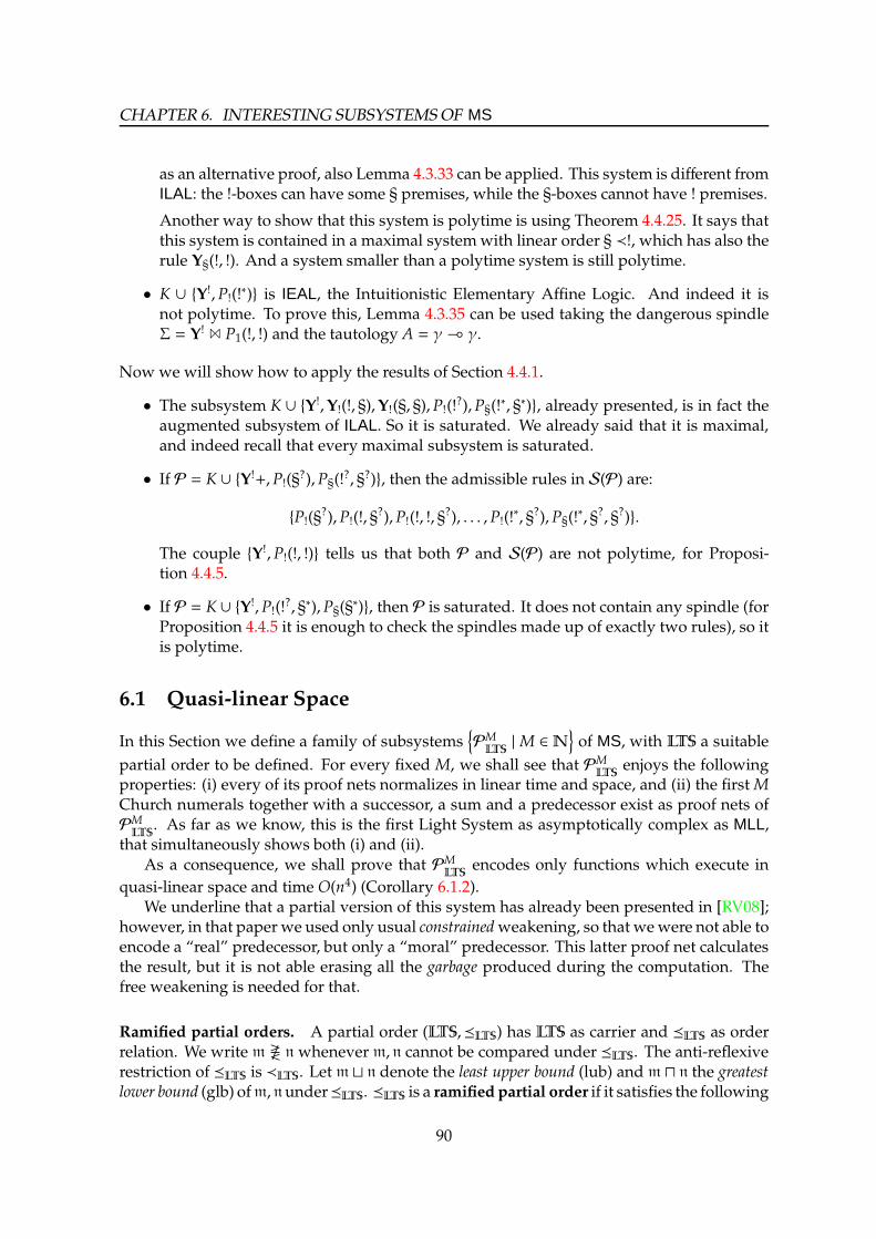
CHAPTER 6. INTERESTING SUBSYSTEMSOF MS
as an alternative proof, also Lemma 4.3.33 can be applied. This system is different fromILAL: the !-boxes can have some § premises, while the §-boxes cannot have ! premises.
Another way to show that this system is polytime is using Theorem 4.4.25. It says thatthis system is contained in a maximal systemwith linear order § ≺!, which has also therule Y§(!, !). And a system smaller than a polytime system is still polytime.
• K ∪ Y!,P!(!∗) is IEAL, the Intuitionistic Elementary Affine Logic. And indeed it is
not polytime. To prove this, Lemma 4.3.35 can be used taking the dangerous spindleΣ = Y!
1 P1(!, !) and the tautology A = γ⊸ γ.
Now we will show how to apply the results of Section 4.4.1.
• The subsystem K ∪ Y!,Y!(!, §),Y!(§, §),P!(!?),P§(!∗, §∗), already presented, is in fact the
augmented subsystem of ILAL. So it is saturated. We already said that it is maximal,and indeed recall that every maximal subsystem is saturated.
• If P = K ∪ Y!+,P!(§?),P§(!?, §?), then the admissible rules in S(P) are:
P!(§?),P!(!, §
?),P!(!, !, §?), . . . ,P!(!
∗, §?),P§(!∗, §?, §?).
The couple Y!,P!(!, !) tells us that both P and S(P) are not polytime, for Proposi-tion 4.4.5.
• If P = K ∪ Y!,P!(!?, §∗),P§(§∗), then P is saturated. It does not contain any spindle (for
Proposition 4.4.5 it is enough to check the spindles made up of exactly two rules), so itis polytime.
6.1 Quasi-linear Space
In this Section we define a family of subsystemsPMLTS| M ∈N
of MS, with LTS a suitable
partial order to be defined. For every fixed M, we shall see that PMLTS
enjoys the followingproperties: (i) every of its proof nets normalizes in linear time and space, and (ii) the firstMChurch numerals together with a successor, a sum and a predecessor exist as proof nets ofPMLTS
. As far as we know, this is the first Light System as asymptotically complex as MLL,that simultaneously shows both (i) and (ii).
As a consequence, we shall prove that PMLTS
encodes only functions which execute in
quasi-linear space and time O(n4) (Corollary 6.1.2).We underline that a partial version of this system has already been presented in [RV08];
however, in that paper we used only usual constrainedweakening, so that wewere not able toencode a “real” predecessor, but only a “moral” predecessor. This latter proof net calculatesthe result, but it is not able erasing all the garbage produced during the computation. Thefree weakening is needed for that.
Ramified partial orders. A partial order (LTS,LTS) has LTS as carrier and LTS as orderrelation. We write m 6R n whenever m, n cannot be compared under LTS. The anti-reflexiverestriction of LTS is ≺LTS. Let m ⊔ n denote the least upper bound (lub) and m ⊓ n the greatestlower bound (glb) ofm, nunderLTS. LTS is a ramified partial order if it satisfies the following
90
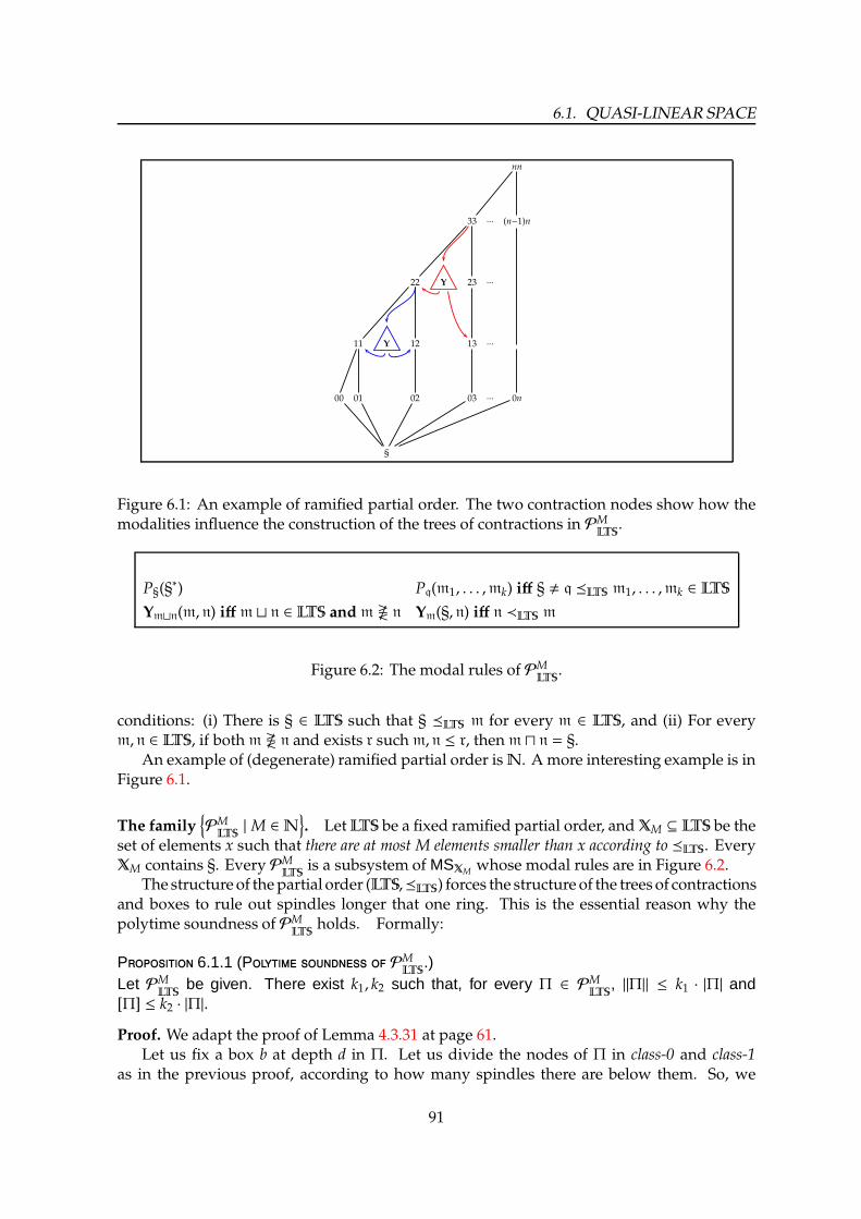
6.1. QUASI-LINEAR SPACE
nn
33 ··· (n−1)n
22 Y 23 ···
11 Y 12 13 ···
00 01 02 03 ··· 0n
§
Figure 6.1: An example of ramified partial order. The two contraction nodes show how themodalities influence the construction of the trees of contractions in PM
LTS.
P§(§∗) Pq(m1, . . . ,mk) iff § , q LTS m1, . . . ,mk ∈ LTS
Ym⊔n(m, n) iff m ⊔ n ∈ LTS and m 6R n Ym(§, n) iff n ≺LTS m
Figure 6.2: The modal rules of PMLTS
.
conditions: (i) There is § ∈ LTS such that § LTS m for every m ∈ LTS, and (ii) For everym, n ∈ LTS, if both m 6R n and exists r such m, n ≤ r, then m ⊓ n = §.
An example of (degenerate) ramified partial order isN. A more interesting example is inFigure 6.1.
The familyPMLTS| M ∈N
. LetLTS be a fixed ramified partial order, andXM ⊆ LTS be the
set of elements x such that there are at most M elements smaller than x according to LTS. EveryXM contains §. Every PM
LTSis a subsystem of MSXM whose modal rules are in Figure 6.2.
The structure of thepartial order (LTS,LTS) forces the structure of the treesof contractionsand boxes to rule out spindles longer that one ring. This is the essential reason why thepolytime soundness of PM
LTSholds. Formally:
P 6.1.1 (P PMLTS
.)Let PM
LTSbe given. There exist k1, k2 such that, for every Π ∈ PM
LTS, ‖Π‖ ≤ k1 · |Π| and
[Π] ≤ k2 · |Π|.
Proof. We adapt the proof of Lemma 4.3.31 at page 61.Let us fix a box b at depth d in Π. Let us divide the nodes of Π in class-0 and class-1
as in the previous proof, according to how many spindles there are below them. So, we
91
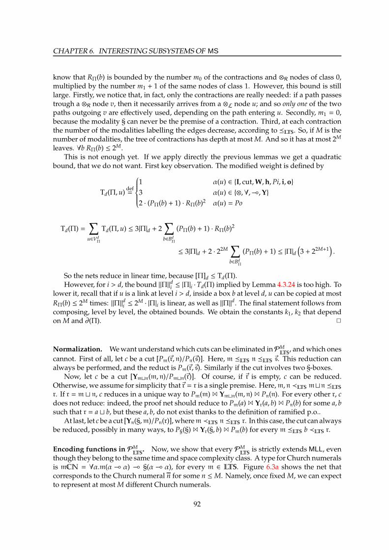
CHAPTER 6. INTERESTING SUBSYSTEMSOF MS
know that RΠ(b) is bounded by the number m0 of the contractions and ⊗R nodes of class 0,multiplied by the number m1 + 1 of the same nodes of class 1. However, this bound is stilllarge. Firstly, we notice that, in fact, only the contractions are really needed: if a path passestrough a ⊗R node v, then it necessarily arrives from a ⊗L node u; and so only one of the twopaths outgoing v are effectively used, depending on the path entering u. Secondly, m1 = 0,because the modality § can never be the premise of a contraction. Third, at each contractionthe number of the modalities labelling the edges decrease, according to LTS. So, if M is thenumber of modalities, the tree of contractions has depth at mostM. And so it has at most 2M
leaves. ∀b RΠ(b) ≤ 2M.This is not enough yet. If we apply directly the previous lemmas we get a quadratic
bound, that we do not want. First key observation. The modified weight is defined by
Td(Π, u)def=
1 α(u) ∈ I, cut,W,h,Pi, i, o
3 α(u) ∈ ⊗,∀,⊸,Y
2 · (PΠ(b) + 1) · RΠ(b)2 α(u) = Po
Td(Π) =∑
u∈VdΠ
Td(Π, u) ≤ 3|Π|d + 2∑
b∈BdΠ
(PΠ(b) + 1) · RΠ(b)2
≤ 3|Π|d + 2 · 22M∑
b∈BdΠ
(PΠ(b) + 1) ≤ |Π|d(3 + 22M+1
).
So the nets reduce in linear time, because [Π]d ≤ Td(Π).However, for i > d, the bound ‖Π‖di ≤ |Π|i ·Td(Π) implied by Lemma 4.3.24 is too high. To
lower it, recall that if u is a link at level i > d, inside a box b at level d, u can be copied at most
RΠ(b) ≤ 2M times: ‖Π‖di ≤ 2M · |Π|i is linear, as well as ‖Π‖d. The final statement follows fromcomposing, level by level, the obtained bounds. We obtain the constants k1, k2 that dependonM and ∂(Π). 2
Normalization. Wewant understandwhich cuts can be eliminated inPMLTS
, andwhich ones
cannot. First of all, let c be a cut [Pm(~r, n)/Pn(~s)]. Here, m LTS n LTS ~s. This reduction canalways be performed, and the reduct is Pm(~r,~s). Similarly if the cut involves two §-boxes.
Now, let c be a cut [Ym⊔n(m, n)/Pm⊔n(~r)]. Of course, if ~r is empty, c can be reduced.Otherwise, we assume for simplicity that~r = r is a single premise. Here,m, n ≺LTS m⊔n LTSr. If r = m ⊔ n, c reduces in a unique way to Pm(m) 1 Ym⊔n(m, n) 1 Pn(n). For every other r, cdoes not reduce: indeed, the proof net should reduce to Pm(a) 1 Yr(a, b) 1 Pn(b) for some a, bsuch that r = a ⊔ b, but these a, b, do not exist thanks to the definition of ramified p.o..
At last, let cbe a cut [Yn(§,m)/Pn(r)], wherem ≺LTS n LTS r. In this case, the cut can alwaysbe reduced, possibly in many ways, to P§(§) 1 Yr(§, b) 1 Pm(b) for every m LTS b ≺LTS r.
Encoding functions in PMLTS
. Now, we show that every PMLTS
is strictly extends MLL, eventhough they belong to the same time and space complexity class. A type for Church numeralsis mCN = ∀α.m(α⊸ α) ⊸ §(α⊸ α), for every m ∈ LTS. Figure 6.3a shows the net thatcorresponds to the Church numeral n for some n ≤M. Namely, once fixedM, we can expectto represent at mostM different Church numerals.
92
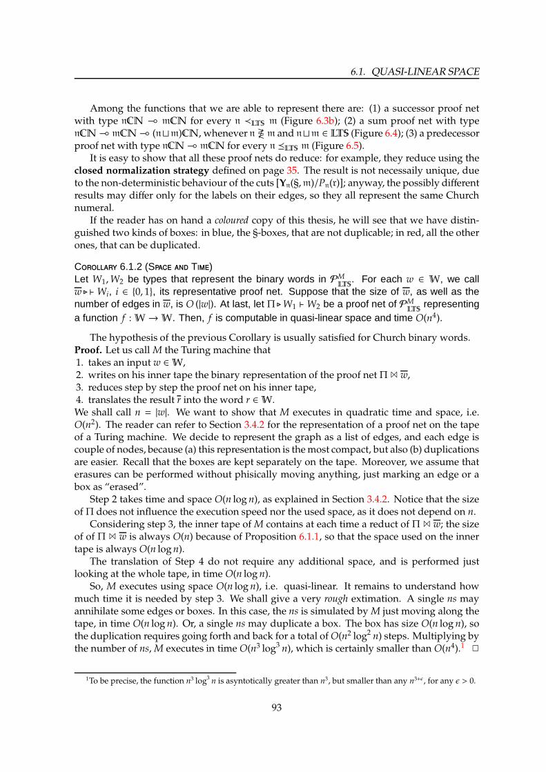
6.1. QUASI-LINEAR SPACE
Among the functions that we are able to represent there are: (1) a successor proof netwith type nCN ⊸ mCN for every n ≺LTS m (Figure 6.3b); (2) a sum proof net with typenCN⊸ mCN⊸ (n⊔m)CN, whenever n 6R m and n⊔m ∈ LTS (Figure 6.4); (3) a predecessorproof net with type nCN⊸ mCN for every n LTS m (Figure 6.5).
It is easy to show that all these proof nets do reduce: for example, they reduce using theclosed normalization strategy defined on page 35. The result is not necessaily unique, dueto the non-deterministic behaviour of the cuts [Yn(§,m)/Pn(r)]; anyway, the possibly differentresults may differ only for the labels on their edges, so they all represent the same Churchnumeral.
If the reader has on hand a coloured copy of this thesis, he will see that we have distin-guished two kinds of boxes: in blue, the §-boxes, that are not duplicable; in red, all the otherones, that can be duplicated.
C 6.1.2 (S T)Let W1,W2 be types that represent the binary words in PM
LTS. For each w ∈ W, we call
w ⊲ ⊢Wi, i ∈ 0, 1, its representative proof net. Suppose that the size of w, as well as thenumber of edges in w, is O (|w|). At last, let Π ⊲W1 ⊢W2 be a proof net of PM
LTSrepresenting
a function f :W→W. Then, f is computable in quasi-linear space and time O(n4).
The hypothesis of the previous Corollary is usually satisfied for Church binary words.Proof. Let us call M the Turing machine that1. takes an input w ∈W,2. writes on his inner tape the binary representation of the proof net Π 1 w,3. reduces step by step the proof net on his inner tape,4. translates the result r into the word r ∈W.We shall call n = |w|. We want to show that M executes in quadratic time and space, i.e.O(n2). The reader can refer to Section 3.4.2 for the representation of a proof net on the tapeof a Turing machine. We decide to represent the graph as a list of edges, and each edge iscouple of nodes, because (a) this representation is themost compact, but also (b) duplicationsare easier. Recall that the boxes are kept separately on the tape. Moreover, we assume thaterasures can be performed without phisically moving anything, just marking an edge or abox as “erased”.
Step 2 takes time and space O(n log n), as explained in Section 3.4.2. Notice that the sizeof Π does not influence the execution speed nor the used space, as it does not depend on n.
Considering step 3, the inner tape of M contains at each time a reduct of Π 1 w; the sizeof of Π 1 w is always O(n) because of Proposition 6.1.1, so that the space used on the innertape is always O(n logn).
The translation of Step 4 do not require any additional space, and is performed justlooking at the whole tape, in time O(n log n).
So, M executes using space O(n log n), i.e. quasi-linear. It remains to understand howmuch time it is needed by step 3. We shall give a very rough extimation. A single ns mayannihilate some edges or boxes. In this case, the ns is simulated by M just moving along thetape, in time O(n log n). Or, a single ns may duplicate a box. The box has size O(n log n), sothe duplication requires going forth and back for a total ofO(n2 log2 n) steps. Multiplying bythe number of ns,M executes in time O(n3 log3 n), which is certainly smaller than O(n4).1 2
1To be precise, the function n3 log3 n is asyntotically greater than n3, but smaller than any n3+ǫ, for any ǫ > 0.
93

CHAPTER 6. INTERESTING SUBSYSTEMSOF MS
o
∀R
⊸R
§R
⊸R
I
⊸L I
⊸L I
⊸L I
§L §L §L
Y Y Y W
∀α.mm(α⊸α)⊸§(α⊸α)=mmCN
mm(α⊸α)⊸§(α⊸α)
§(α⊸α)
α
α⊸α
α⊸α
α⊸α
mm−1(α⊸α)m1(α⊸α)
mm(α⊸α)
(a) A Church numeral less than m.
o
⊸R
∀R
⊸R
§R
⊸R
I
⊸L I
⊸L I
§L §L
⊸L I
∀L Y
nCN⊸mCN (n≺LTSm)
∀α.m(α⊸α)⊸§(α⊸α)
m(α⊸α)⊸§(α⊸α)
§(α⊸α)
α⊸α
α
α
α
α⊸α
α⊸α
§(α⊸α)
n(α⊸α)⊸§(α⊸α)§(α⊸α)
n(α⊸α)
(b) Successor on Church numerals
Figure 6.3: PMLTS
: encoding Church numerals and successor.
94

6.1. QUASI-LINEAR SPACE
o
⊸R
⊸R
∀R
⊸R
§R
⊸R
I
⊸L I
⊸L I
§L §L
⊸L I ⊸L I
∀L ∀L
Y
nCN⊸mCN⊸(n⊔m)CN (n6Rm,n⊔m∈LTS)
mCN⊸(n⊔m)CN
(n⊔m)CN
(n⊔m)(α⊸α)⊸§(α⊸α)
§(α⊸α)
α⊸α
α
α
α
α
α⊸α
n(α⊸α)⊸§(α⊸α) m(α⊸α)⊸§(α⊸α)
n(α⊸α)
m(α⊸α)
(n⊔m)(α⊸α)
Figure 6.4: PMLTS
: the sum of two Church numerals of type nCN,mCN with n 6R m andn ⊔m ∈ LTS.
95
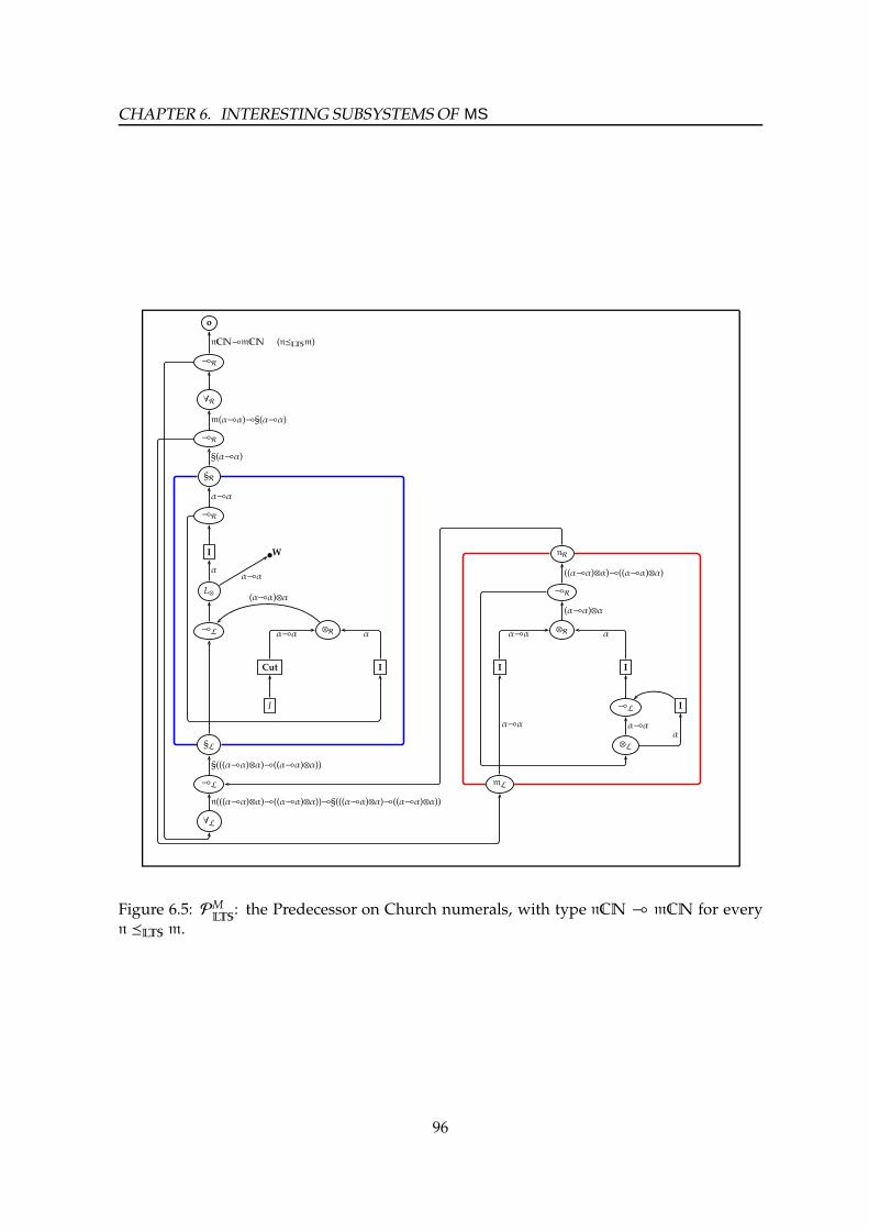
CHAPTER 6. INTERESTING SUBSYSTEMSOF MS
o
⊸R
∀R
⊸R
§R
⊸R
I W nR
L⊗ ⊸R
⊸L ⊗R ⊗R
Cut I I I
I ⊸L I
§L ⊗L
⊸L mL
∀L
nCN⊸mCN (nLTSm)
m(α⊸α)⊸§(α⊸α)
§(α⊸α)
α⊸α
((α⊸α)⊗α)⊸((α⊸α)⊗α)αα⊸α
(α⊸α)⊗α
(α⊸α)⊗α
α⊸α α α⊸α α
α⊸αα
§(((α⊸α)⊗α)⊸((α⊸α)⊗α))
α⊸α
n(((α⊸α)⊗α)⊸((α⊸α)⊗α))⊸§(((α⊸α)⊗α)⊸((α⊸α)⊗α))
Figure 6.5: PMLTS
: the Predecessor on Church numerals, with type nCN ⊸ mCN for everyn LTS m.
96

6.2. SOLAL
Pi!(i!?, j1§∗, . . . , jm§∗) for every j1, . . . , jm < i ≤MPi§(i!∗, i§∗, j1§∗, . . . , jm§∗) for every j1, . . . , jm < i ≤M
Yi!(i!, i!) for every i ≤M
Figure 6.6: The modal rules of soLALM.
⊸R
i!R
I
⊸L 0
j§L
⊸L
⊸L j!R j!R
∀L succ0 succ1
jW⊸i!(kW)
i!(kW)
kW⊸kW
j§(kW⊸kW)
kW
j!(kW⊸kW)
j!(kW⊸kW)
Figure 6.7: The proof nets Crc j<i,k in soLAL, with j < i, for any k.
6.2 soLAL
We have pointed out, many times, that we are interested in finding some subsystemP ⊆ MSable to represent as many SRN programs as possible. soLAL is designed precisely withthis target in mind. See Section 2.7 for a definition of SRN. Firstly, we will define a familyof subsystems soLALM ⊆ BY, with Y = i! | i ≤ M ∪ i§ | i ≤ M for some fixed M ≥ 2.Every one of such subsystems is a proper extension of ILAL. Later we encode a fragmentSRN– of SRN into soLALM (Proposition 6.2.5). The more, we will come to the same resultthrough twodifferent encodings (Lemma6.2.7and 6.2.8); this, togetherwith some concludingobservations in Section 6.3, suggests that the complexity of soLAL is really the one of SRN–,whatever encodingwe choose. The details of the encodingwill be postponed toAppendixA,for the very interested reader only, because of its length.
Definitions. soLALM (soLAL for short) contains the linear kernel of MS, plus the modalrules in Figure 6.6. Figure 6.7 shows an example of proof net we can build in soLAL but notin ILAL. Themeaning of such a proof net will be explained later on. Exactly as in the previousSection 6.1, if the reader has on hand a coloured copy of this thesis, he will see that we have
97

CHAPTER 6. INTERESTING SUBSYSTEMSOF MS
distinguished two kinds of boxes: in blue, the §-boxes, that are not (directly) duplicable; inred, the !-boxes, that canbeduplicated. Thename soLAL stands for sorted ILAL, because soLALextends ILAL with the introduction of sorted modalities. For example, every i!(α⊸ α) is anof-course (modal) formula of sort i, and i§(α⊸ α) is a paragraph one of sort i. i§nA abbreviatesi§· · · i§A, with n ≥ 0 occurrences of i§. An analogousmeaning holds for i!nA. We observe thatrestricting Pi!(i!
?, j1§∗, . . . , jm§∗) to Pi!(i!?), and Pi§(i!
∗, i§∗, j1§∗, . . . , jm§∗) to Pi§(i!∗, i§∗) we get a
subsystem i- soLAL of soLAL. Every i-soLAL is ILAL identifying !A ≡ i!A, i§B ≡ §B, for everyA,B.
Basic properties. Let R↑ the preordering among the modalities of soLALM defined in Sec-tion 4.4.2. Observing that the preordering in this case is in fact a linear ordering, we under-stand that in soLALM it is not possible to build dangerous spindles, so:
F 6.2.1For every fixed M, soLALM is polytime.
R 6.2.2 soLAL does not enjoy cut-elimination, because e.g. a cut Pi!( j§) 1 Yi! cannotreduce.
soLAL is not confluent as well, because the two cuts Pi!( j§) 1 Pi!(i!) 1 Yi! can both reduceto different normal forms. (By the way, we have used Lemma 5.2.1 to find out such anexample). Here we want to remark why the above two negative aspects, which relate to soLALtaken in its generality, are harmless in the case we consider. Indeed, we can certainly adopt theclosed normalization strategy, already defined on page 35: reduce one instance of the cuts[P/P], [P/Y] only if the lowermost box they involve is closed. All the reductions that we needmay be performed using such a strategy. Moreover, the normal form we end up with isunique.
Anyway, we conjecture that such a normalization strategy can in fact be avoided, for wefocus on a very a specific set of proof nets that soLAL can contain.
soLAL can prove j§A⊸ i!A, for j < i and for every A. This is its most important feature.This is the reason why soLAL generalizes ILAL: ILAL can prove !A⊸ §A, but not §A⊸ !A.
In soLAL we can define iW = ∀α.i!(α⊸ α) ⊸ i!(α⊸ α) ⊸ i§(α⊸ α) as the type of(Church) (binary) words of sort i, and iS = ∀α.i!(α⊸ α)⊸ i§(α⊸ α) as the i-sort type of (unary)strings. Also, from ILAL we recall that a word-coercion proof net, of type W ⊸ § †W forany sequence of modalities †, takes a word as argument to rebuild it inside some boxes, theoutermost being a §-box. In ILAL, the outermost box can only be §. Instead, the type of theword-coercion proof nets of soLAL can be also jW ⊸ i!(†kW), for every j < i, k ∈ N, as inFigure 6.7. Please, notice i! in front of kW. soLAL is a kind of hierarchy of systems i-soLALthat can “communicate” at least by word-coercion proof nets that map words from one levelto the other.
The restrictions SRN= and SRN– of SRN. The reader can find the definitions of recursion,linear recursion and linear composition in Figure 2.5.
D 6.2.3 SRN= is the set containing BC–, plus all the functions that can be obtainedfrom BC– with 1 application of (not necessarily linear) Safe Recursion.
98

6.2. SOLAL
Namely, like in BC–, we allow in SRN= arbitrarily nested linear recursions; moreover, weallow the outermost recursion to be non-linear. Moreover, the functions obtained usingan outermost recursion can be further linearly composed. As an example, the followingprogram g is in SRN– but not in BC–. We omit the projections, to lighten the presentation:
h(w; y, z, t) = cond( ;w, y, t)g(0; y, z) = z (∗)
g(siw; y, z) = h(w; y, z, g(w; y, z))
The program g(w; y, z) returns y if w , 0 contains a digit ’0’ that is not the lowermost digit,and z otherwise.
D 6.2.4 SRN– is the least set containing BC–, closed under Safe Linear Composi-tion, and closed under Safe Recursion limited to any g, h0, h1 ∈ BC–.
For example, if g(w; y, z) is as in (*), then h(w; y, z) = si( ; g(w; y, z)) is in SRN–.It holds BC– ( SRN= ( SRN– ( SRN. Our goal is to focus on SRN–; SRN= is only
useful to identify some functions of SRN– crucial for our proofs. The theorem we want toprove is the following:
P 6.2.5 (F SRN– soLAL.)
There is a compositional map p·q from SRN– to soLAL, such that for every f ∈ SRN theproof net p fq represents f .
In the next paragraphs we provide two different proofs for it.
FollowingMurawski-Ong’s encoding. Wewill prove Proposition 6.2.5 using an encodingperfectly analogous to the one of [MO04]. We shall see that it is possible, in that way, toencode some non-linear recursion; however their type is not further iterable, so that we arenot able representing the whole SRN but only its fragment SRN–.
L 6.2.6 (BC– soLAL)
Every function f ∈ (BC–)n;s can be represented in soLAL with type:
p fq ⊲ j1W, . . . , jnW, j§m(kW), . . . , j§m(kW)︸ ︷︷ ︸
s
⊢ j§m(kW)
for every j, k, every j1, . . . , jn, j ≤ j and every m big enough.
Proof. If we follow exactly [MO04], we get an encoding in which all the sorts are equal:j1 = . . . = jn = j = k. Here we can be more flexible on the sorts, because soLAL has, inparticular, the promotion rule j§m(kW)⊸ k§m(kW) and the coercion j1W⊸ k§(kW). 2
L 6.2.7 (N- R soLAL, #1)Let us assume that g ∈ SRNn;s and h0, h1 ∈ SRN1+n;s+1 can all be represented in soLAL withproof nets:
ph0q, ph1q ⊲ (⊸nr=0 jrW)⊸ (⊸s
r=1 j§m(kW))⊸ j§m(kW)⊸ j§m(kW)
pgq ⊲ (⊸nr=1 jrW)⊸ (⊸s
r=1 j§m(kW))⊸ j§m(kW) .
99

CHAPTER 6. INTERESTING SUBSYSTEMSOF MS
for some j0, . . . , jn, j, k,m. Then, it is also possible to encode the function f ∈ SRN1+n;s
obtained by Recursion of g, h0, h1 as a proof net p fq of soLAL, whose type is:
p fq ⊲ (⊸nr=0 jrW)⊸ (⊸s
r=1 i§m+2(kW))⊸ j§m+2(kW) ,
for every i < j.
Proof. The construction that proves this Lemma is in Figure 6.8. Please notice that such aproof net contains some irreducible cuts; anyway, the proof net obtained cutting the non-linear recursion with some numerals is closed, and thus it can be reduced starting from theclosed boxes. 2
Proof of Proposition 6.2.5. Lemma 6.2.6 shows how to represent the functions of BC–
in soLAL. Lemma 6.2.7 shows that it is then possible to apply a non-linear recursion, thusrepresenting in soLAL allSRN=. Now,wewant to linearly compose theSRN= functions, thusgetting the SRN– functions. This is possible thanks to the type provided by Lemma 6.2.7.Indeed, imagine wewant to cut a function f with output type j§m(kW) with a function gwithsafe input type i§m(kW). Lemma 6.2.7 assures that, in this situation, f can also be written asanother proof net f ′ with output type i§m(kW), changing also its input types. Hence we cancompose gwith f ′. 2
A different encoding. As we anticipated, we have proved the same Proposition 6.2.5 fol-lowing two completely different approaches. Here, we show the second one. Instead ofusing Lemma 6.2.7, we use the forthcoming Lemma 6.2.8. All the remaining parts of theproof of Proposition 6.2.5 are identical.
Notice that the only difference between Lemma 6.2.7 and Lemma 6.2.8 is in the type ofthe got proof net. The encoding, that here we just sketch, exploits the use of the boxes of typej§A⊸ i!B, sowewould expect to reach a result better than the one of Lemma 6.2.7. However,this is false. The functions that we got still are non-iterable, so that we again encode the sameset of functions SRN–.
L 6.2.8 (N- R soLAL, #2)Let us assume that g ∈ SRNn;s and h0, h1 ∈ SRN1+n;s+1 can all be represented in soLAL withproof nets:
ph0q, ph1q ⊲ (⊸nr=0 jrW)⊸ (⊸s
r=1 j§m(kW))⊸ j§m(kW)⊸ j§m(kW)
pgq ⊲ (⊸nr=1 jrW)⊸ (⊸s
r=1 j§m(kW))⊸ j§m(kW) .
for some j,m. Then, it is also possible to encode the function f ∈ SRN1+n;s as a proof netp fq of soLAL, whose type is:
p fq ⊲ (⊸nr=0 jrW)⊸ (⊸s
r=1 i§3 j§m+1(kW))⊸ i§4 j§m(kW) ,
for every i > j.
The encoding that allows the proof of Lemma 6.2.8 is quite heavy. Here we just sketchthe main ideas. Details can be found in Appendix A.
The embedding p·q is inductively defined on the structure of its argument. We willdescribe how to build p f 1+n;sq in the case that f 1+n;s is (not necessarily linear) recursive, i.e.
100

6.2. SOLAL
j§
Π
⊸L
⊗R
0 I Lift [g]
Y Y
∀L j0§ j1§ j§
Cut ⊸L Step1 Cut Cut
reverse ⊸L Step0 coerce
j§m+2(kW)
j§m+1(kW)
A
A⊸A
A
j!( j0W) j§m+1(kW)
j!( j1W) j! j§m(kW)
j!( j1W)
j!( j1W)
I
j! j§m(kW)
j1W
j1§ j!( j1W)
j§ j! j§m(kW)
i§m+2(kW)
j0W
j0W
j0!(A⊸A)
j0!(A⊸A)
(a) Safe and Linear Recursion
j0!
⊸R
⊗R
succi I Lift [hi]
Y Y Y
⊗L
j0!(A⊸A)
A⊸A
A
j!( j0W)j!( j1W) j! j§m(kW)
j§m+1(kW)
j!( j0W)
j!( j0W)
j!( j1W)
I
j§m+1(kW)
(b) Stepi
wherewe assume n = s = 1,Π is projection of its last argument, ⊗R and ⊗L are sequences
of ⊗R and ⊗L nodes resp., Stepi, with i ∈ 0, 1, is on the right, and
A = j!( j0W) ⊗ . . . ⊗ j!( jnW) ⊗ j! j§m(kW) ⊗ . . . ⊗ j! j§m(kW)︸ ︷︷ ︸
s
⊗ j§m+1(kW).
Figure 6.8: The safe not necessarily linear recursion proof net in soLAL. We assume thatn = s = 1.
of type (2.10), built on g, h0, h1. Instead, if f is basic or it is a linear composition, it is enoughto follow [MO04] that defines the map from BC– to ILAL.
p f (w,−→xn;−→y
s)q iterates ph0q, ph1q as many times as the length of w, from an initial
pg(−→xn;−→y
s)q. In order to do this, p f (w,−→x
n;−→y
s)q maintains a configuration, that changes
at each step; a configuration can be ideally represented as a tuple
〈r, [a1, . . . , ar], [x11, . . . , x1r], . . . , [xn1, . . . , xnr], [y11, . . . , y1r], . . . , [ys1, . . . , ysr]〉
The word r is initially pg(−→xn;−→y
s)q, then step-by-step accumulates the result of the recursion
unfolding. The remaining elements of the configuration are lists of words, all with length r;at the beginning, r = |w| + 1, then the lists are consumed along the computation.
Anexample. Wegive a simple example of the role of the configurations to represent p f 1+n;sq.
Let n = 0, s = 1, G = pgq, Hi = phiq, with i ∈ 0, 1, 0 = p0q, and a = paq. Let a possible
101
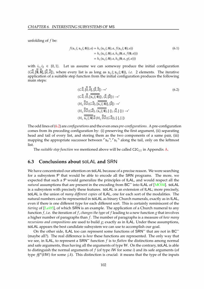
CHAPTER 6. INTERESTING SUBSYSTEMSOF MS
unfolding of f be:
f (si1(; si2(; 0)); a) = hi1(si2(; 0); a, f (si2(; 0); a)) (6.1)
= hi1(si2(; 0); a, hi2(0; a, f (0; a)))
= hi1(si2(; 0); a, hi2(0; a, g(; a)))
with i1, i2 ∈ 0, 1. Let us assume we can someway produce the initial configuration
〈Ga, [0, 0], [a, a]〉, where every list is as long as si1 (; si2(; 0)), i.e. 2 elements. The iterativeapplication of a suitable step function from the initial configuration produces the followingmain steps:
〈Ga, [0, 0], [a, a]〉 →∗ (6.2)
〈Ga, 〈0, [si2(; 0)]〉, 〈a, [a]〉〉 →∗
〈Hi2 0 a (Ga), [si2(; 0)], [a]〉 →∗
〈Hi2 0 a (Ga), 〈si2(; 0), [·]〉, 〈a, [·]〉〉 →∗
〈Hi1 si2(; 0) a (Hi2 0 a (Ga)), [·], [·]〉
Theodd lines of (6.2) are configurationsand the evenones pre-configurations. Apre-configurationcomes from its preceding configuration by: (i) preserving the first argument, (ii) separatinghead and tail of every list, and storing them as the two components of a same pair, (iii)mapping the appropriate successor between ps0q, ps1q along the tail, only on the leftmostlist.
The suitable step function we mentioned above will be called C2C1;1 in Appendix A.
6.3 Conclusions about soLAL and SRN
Wehave concentrated our attention on soLAL because of a precise reason. Wewere searchingfor a subsystem P that would be able to encode all the SRN programs. The more, weexpected that such a P would generalize the principles of ILAL, and would respect all thenatural assumptions that are present in the encoding from BC– into ILAL of [MO04]. soLALis a subsystem with precisely these features. soLAL is an extension of ILAL; more precisely,soLAL is the union of many different copies of ILAL, one for each sort of the modalities. Thenatural numbers can be represented in soLAL as binary Church numerals, exactly as in ILAL,even if there is one different type for each different sort. This is certainly reminiscent of thetiering of [Lei93], of which SRN is an example. The application of a Church numeral to anyfunction f , i.e. the iteration of f , changes the type of f leading to a new function g that involvesa higher number of paragraphs than f . The number of paragraphs is a measure of how manyrecursions and compositions are used to build g; exactly as in ILAL. Under these assumptions,soLAL appears the best candidate subsystemwe can use to accomplish our goal.
On the other side, ILAL too can represent some functions of SRN– that are not in BC–
(maybe all?). The real difference is how these functions are represented. The only way thatwe see, in ILAL, to represent a SRN– function f is to flatten the distinctions among normaland safe arguments, thus having all the arguments of typeW. On the contrary, soLAL is ableto distinguish the normal arguments of f (of type iW for some i) and its safe arguments (oftype j§m(kW) for some j, k). This distinction is crucial: it means that the type of the inputs
102

6.3. CONCLUSIONS ABOUT SOLAL AND SRN
and of the output of f is (almost) preserved. This is in accordance with the intuition: thenumber m of paragraphs in the type of the output of f , that is equal to number of paragraphs in thetype of the safe arguments, is a measure of the complexity of f . Namely, it is a bound on the numberof nested recursion and composition schemes occurring in f .
Now, soLAL is anyway not able to represent the whole SRN. This suggests some consid-erations. Let us focus for a moment on the theorems j§A⊸ i!A, for j < i, that are provable insoLAL. These implications are a kind of inverse of the theorems !A⊸ §A, typical of ILAL. But,of course, ILAL and soLAL cannot prove §A ⊸ !A because this theorem would break theirpolynomial time soundness. We like to imagine all the theorems j§A⊸ i!A as approximationsof §A ⊸ !A. Every such approximation is compatible with the polynomial time soundness,while its upper bound §A⊸ !A is not. This approach suggests that soLAL is the best subsystemof MS that extends ILAL under the natural assumptions we mentioned above.
A pair of words about other, possible, subsystems of MS encoding SRN. We have triedlots of them, without getting any result better than the one of soLAL. Just as an example,we can imagine a subsystem based on PM
LTSof Section 6.1, where the numerals are encoded
using asymmetric contractions. Of course this approach — as all the other ones we canimagine — is quite different from ILAL, thus getting far from the assumptions we underlinedat the beginning of this Section. This is why we preferred to omit from this thesis all theseattempts. Only a few of them— theonesmore strictly relatedwith soLAL—will be discussedin Section 8.1.
103

CHAPTER 6. INTERESTING SUBSYSTEMSOF MS
104

Chapter 7
An alternative approach: LALL
We have already seen that it is an interesting challenge to represent SRN programs insidesome subsystem of MS. This was, in fact, the main motivation that led us to the study of MS.However, we did not reach our goal. We identified some subsystems that slightly extend theexpressiveness of ILAL, but none of them is really able to capture the whole SRN. It appearslike that the stratification property, that is fundamental for ILAL, is too strong w.r.t. SRN.
In this last Chapter we will partially solve the problem using a different approach. Wewill present a polytime logic LALL that extends ILAL using both the levels of L4, and somerecursive types. We will be able to compositionally encode into LALL all the finite initialfragments of all the SRN programs (Proposition 7.5.2). LALL is not a subsystem of MS.LALL is not stratified, but anyway it is weakly stratified, i.e. it satisfies a weaker notionof stratification. When we say weakly stratified, we do not refer to the property of WeakStratification as defined in [BM10], that strictly depends on the syntax of proof nets they use.More simply, we refer to the fact that, during a reduction, the residues of any node u areeither at the same depth or at the same level of u (Fact 7.1.4).
We strongly suggest the reader to read the summary of this Chapter at page 9, before thisChapter itself, where we have underlined the most important features of LALL.
One possible objection is the following. Apparently, in this way, it is possible to representin LALL every total function, even the non-computable ones. Indeed, if f is a non-computabletotal function, and f l is a finite initial fragment of f , then f l is also an initial fragment ofsome SRN program tl, so f l can be represented in LALL, and at last we have representedf in LALL. However, we underline two facts. (i) The representation just given for f is nonconstructive, as we do not know which tl can represent f . (ii) We are not interested in thefunctions, but in the algorithms. It is not possible to represent every algorithm in LALL, but atleast it is possible to represent the SRN ones.
The previous observations are supported by the forthcoming Lemma 7.4.2. It shows that,in fact, all the functions g : W → W eventually constant can be easily represented in LALL.Eventual constant means constant for all but finitely many inputs. Every such a function iscomputable in constant time, so it is not surprising that they can be encoded in whateverlogic. Anyway, g is encoded using a naıve look-up algorithm, so that (a) the embeddingis all but compositional, (b) the proof net required to encode g has really large size, andfinally (c) Lemma 7.4.2 is useless in a complexity perspective, andwe cannot use it for provingProposition 7.5.2.
105

CHAPTER 7. AN ALTERNATIVE APPROACH: LALL
I
A
A
Cut
A
A W
AhA Y
!A !A
!A
⊗L
A⊗B
A B
⊗RA B
A⊗B
Identityor Axiom
Cut Weakening Dæmon Contraction Tensor L Tensor R
∀L
∀α.A
A[B/α]
∀R
A
∀α.A
⊸L
B
A⊸BA
⊸R
B
A⊸BA
!
!A
A
!
A
!A
§
§A
A
§
A
§A
For all L For all R Implication L Implication R Bang L Bang R Paragraph L Paragraph R
Figure 7.1: The nodes in the proof nets of LALL.
7.1 Light Affine Logic by Levels
The language of formulæ. First, for any fixed countable setV of propositional variables,the set F of formulæ is generated by the following grammar:
F : :=S | α | F ⊗ F | F⊸ F | ∀α.F | !F | §F α ∈ V
where S is a constant. Second, we define the quotient FS of F by assuming:
S = ∀α.(α⊸ (B⊸ S ⊸ α)⊸ α) (7.1)
among the elements of F . Namely, (7.1) gives to S the meaning of Scott numerals [ACP93].The formulæ we shall effectively use are the equivalence classes in FS . Every time we labelan edge of a proof net of LALL by S , we can also label that edge by any “unfolding” of S
that obeys (7.1). B[C/α]is the substitution of every free occurrence of α in Bwith C. Similarly,
(∀α.A)Cmeans A[C/α].
Proof structures and proof nets. LALL is a language of proof nets. Proof nets are defined,essentially, as for MS. For sake of simplicity, we will recall them here. Given the nodes inFigure 7.1, we say that an Axiom node and a Dæmon nodes are proof structures. Moreover, giventwo proof structuresΠ and Σ:
Π
......A1 Ar
C
Σ
......B1 Bl
D
denoted as Π ⊲ A1, . . . ,Ar ⊢ C and Σ ⊲ B1, . . . ,Bl ⊢ D, respectively, with r, l ≥ 0, then all thegraphs inductively built fromΠ and Σ by the rule schemes in Figure 7.3 are proof structures.
Now, indexing is introduced, exactly as in Section 8.2.2.
D 7.1.1 (I P , [BM10]) Let Π be a proof struc-ture.
1. An indexing forΠ is a function I from the edges ofΠ toZ that satisfies the constraintsin Figure 7.2 and such that I(e) = I(e′), for every pair e, e′ of inputs and output of Π.
2. A proof net is a proof structure that admits an indexing.
106

7.1. LIGHT AFFINE LOGIC BY LEVELS
!
i
i+1
!
i+1
i
§
i
i+1
§
i+1
i
Figure 7.2: Constraints on the indexing. The nodes we omit have the same index on all oftheir incident edges.
3. An indexing I ofΠ is canonical ifΠ has an edge e such that I(e) = 0, and I(e′) ≥ 0 for alledges e′ of Π.
F 7.1.2 (E U C I)Every proof net of LALL admits a unique canonical indexing.
The indexing tells that the nodes !L and §L are not standard dereliction nodes. Instead, theyare auxiliary ports of §-boxes whose border is somewhat fuzzy. We mean that a §-boxes isnot necessarily either contained into or disjoint from another box. Instead, it can “overlap”a !-box, and it can have more than one conclusion Paragraph R. To distinguish §-boxes fromthe ! ones we adopt a dotted border (and also a different colour, if the reader is reading acoloured version of this thesis). Please notice that these boxes are completely useless, andthey can be avoided as in [BM10]; anyway, we think they are useful to underline that § and !nodes are not dereliction nodes.
Let I0 be the canonical indexing of Π and e ∈ EΠ. The level of e is l(e). It is defined as I0(e).The level of Π is l(Π). It is defined as the greatest value assumed by I0 on the edges of Π. Wedenote as usual as BΠ the set of the !-boxes in Π, and it is naturally in bijection with the setof the !R nodes in Π.
Normalization. Most of the normalization steps (ns) are analogous to the namesake of MS,already described in Section 3.3. We just recall what they do. The linear normalizationsteps annihilate in the natural way a pair of linear nodes (Identity/Cut, ⊸L / ⊸R, ⊗L/⊗R,§L/§R, ∀L/∀R). The modal normalization steps are of two kinds: !L/!R is reduced mergingthe two involved boxes which can be !-boxes as well as §-boxes fuzzy borders. Instead,contraction/!R duplicates the whole !-box cut with the contraction, as in ILAL. The garbagecollection normalization steps involve the weakening or the dæmon nodes, cut with anyother node. It is always possible to reduce such a cut with the help of some more weakeningand dæmon nodes, as done in ILAL [AR02]. The set of cut nodes of Π is cuts(Π).
F 7.1.3 (C-)Every LALL proof net reduces to some cut-free proof net.
We recall that the definition of stratification is at page 39.
F 7.1.4 (W S)Let Π be a LALL proof net such that Π → Π′ by reducing a cut node at level i and depth d.Let e be any edge in Π, and e′ any one among its residues in Π′. Then, either ∂(e) = ∂(e′), orl(e) = l(e′).
107

CHAPTER 7. AN ALTERNATIVE APPROACH: LALL
Π
Cut
Σ
...
C
A1 ArD
D
B1 Bl
Π
∀L
C
A1
A[B/α]
Ar
∀α.A
∀R
Π
...
∀α.C (∗)
C
A1 Ar
⊸R
Π
A j⊸C
C
A1 ArA j
Π
⊸L
Σ
. . .
C
A1 ArAi
D⊸Ai
D
B1 Bl
⊗R
Π Σ
. . . . . .
C⊗D
C D
A1 Ar B1 Bl
Π
⊗L
C
A1 Ar
Ai A j
Ai⊗A j
Π
§
C
A1
Ai
Ar
§Ai
§
Π
. . .
!C
C
A1 Ar
Π
Y
C
A1 Ar
!A !A
!A
Π W
. . .
C
A1 Ar E
Π
!
C
A1
Ai
Ar
!Ai
!
Π
!
!C
C
A
!A (∗∗)
Figure 7.3: Inductive rule schemes to build proof structures of LALL. (*) α does not occur freein A1, . . . ,Ar. (**) A !-box, which has at most a single assumption.
7.2 LALL is polytime
We adapt the definitions of [BM10], with some minor modifications to handle the free weak-ening nodes. Let us fix a proof net Π to reduce. We define an ordering over cuts(Π) thatdetermines which cuts to reduce first.
A graph theoretic path in any proof net Π is exponential if it contains a, possibly empty,sequence of consecutive contractions and stops at a !L node.
Let B,C ∈ BΠ. Let B ≺L1 C if the roots of B and C lie at the same level, and the root of B is
in cut with an exponential path that enters a left port of C. L is the reflexive and transitiveclosure of ≺L
1. One can show that L is a partial order, upward arborescent: for every C there
is at most one B such that B ≺L1C.
Let c, c′ ∈ cuts(Π). We write c ≤ c′ iff one of the following conditions holds. (i) c′
is connected to a weakening or a dæmon, and c is not. (ii) The condition (i) is false butl(c) < l(c′) holds. (iii) The conditions (i) and (ii) are false, so l(c) = l(c′). In this case, c ≤ c′ iff:(a) either c′ is connected to a contraction, and c is not, or (b) c, c′ are connected to a contractionon one side, to the boxes B,B′, respectively, on the other, and B L B′.
D 7.2.1 (C ) A sequence of normalization steps that startsfrom a given proof netΠ is canonicalwhenever cuts that are smaller under ≤ are eliminatedbefore higher ones.
T 7.2.2 (P LALL)Let Π be a LALL proof net of size s, level l, and depth d. Then, every canonical reduction is
108

7.3. PRELIMINARYNOTIONS ABOUT SRN
long at most (l + 1)s(d+2)lsteps.
The proof strategy coincides with the one in [BM10], where the reduction of the garbagecollection steps is delayed till the end.
7.3 Preliminary notions about SRN
We recall from Section 2.7 that SRNn;s is the subset of SRN whose terms have normal arity
n, and safe arity s. If not otherwise stated, ~tm = t1, . . . , tm will always denote sequences
of m ≥ 0 terms of SRN. Moreover, we write |~tm| ≤ l, for some l > 0, meaning that thesize of every term ti is not greater than l. Now, we recall that, for every t in SRNn;s, and~x = x1, . . . , xn, ~y = y1, . . . , ys, it holds
|t(~x; ~y)| ≤ pt (|x1|, . . . , |xn|) +max|y1|, . . . , |ys|
(7.2)
where pt is the characteristic polynomial of t which is non-decreasing and depends on t. Wenotice that if u is a subterm of t, then deg(pu) ≤ deg(pt), deg(p) denoting the degree of thepolynomial p. At last, we define the composition degree ∂C(t) and the recursion degree ∂R(t) of t,as the functions that count resp. the number of safe composition and of recursion schemesinside t.
D 7.3.1 (O B F ob·(·)) Let t in SRNn;s and l ≥ 0. We defineob·(·), that takes t and l as arguments, as obt(l) = pt(l, . . . , l) + l.
F 7.3.2 (ob·(·) B O L t ∈ SRN)For every t in SRNn;s, l ≥ 0, and sequences ~x, ~y such that |~x|, |~y| ≤ l, we have |t(~x; ~y)| ≤ obt(l).
The following definition will be used only in Proposition 7.5.2. Notice that nbt(l) is a polyno-mial, for every fixed t.
D 7.3.3 (N B F nb·(·)) Let t in SRNn;s and l ≥ 0. We define nb·(·),that takes t and l as arguments, as nbt(l) = obt(obt(. . . obt(l) . . .))︸ ︷︷ ︸
∂R(t)+∂C(t) times
.
We have to deal with various kinds of numbers, so the following correspondence is conve-nient:
F 7.3.4 (R N, S , W--T)Every sequence (d1, . . . , dl) with d1, . . . , dl ∈ 0, 1 and l ≥ 0, identifies uniquely a numbern = 2l−1 · dl + · · ·+ 2
0 · d1 ∈N. So, both the term of SRN sdl(; . . . sd1(; 0) . . .) and the Scott word[n] identify n, too. We say that the sequence, as well as the Scott number and the SRN term,represent n.
We underline that an infinite number of sequences, and of terms, represent the same n.
7.4 Preliminary useful proof nets in LALL
Booleans. The type of booleans is B = ∀γ.γ ⊸ γ⊸ γ whose representative proof nets arein Figure 7.4. The proof net ∇B[b] duplicates any boolean we may plug into b by a Cut node.
109
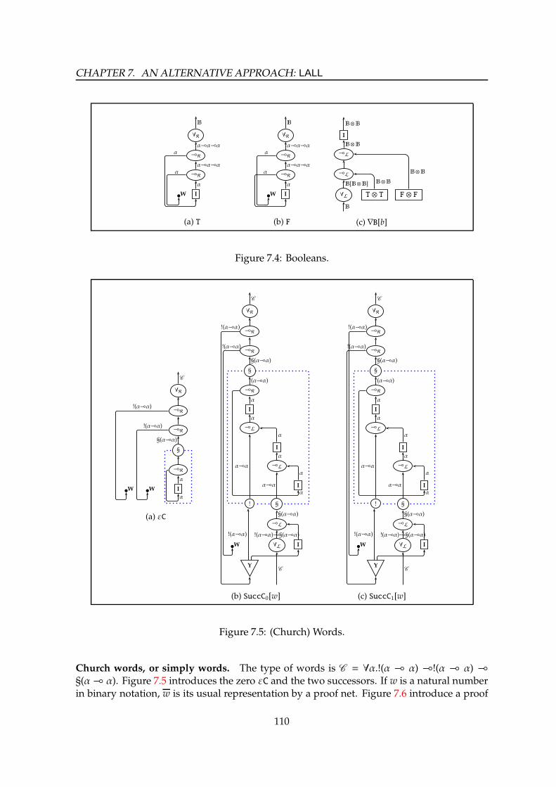
CHAPTER 7. AN ALTERNATIVE APPROACH: LALL
∀R
⊸R
⊸R
W I
B
α⊸α⊸α
α⊸α⊸α
α
α
α
(a) T
∀R
⊸R
⊸R
W I
B
α⊸α⊸α
α⊸α⊸α
α
α
α
(b) F
I
⊸L
⊸L
∀L T ⊗ T F ⊗ F
B⊗B
B⊗B
B[B⊗B] B⊗B
B⊗B
B
(c) ∇B[b]
Figure 7.4: Booleans.
∀R
⊸R
⊸R
§
⊸R
W W I
C
§(α⊸α)
α
!(α⊸α)
!(α⊸α)
α
(a) εC
∀R
⊸R
⊸R
§
⊸R
I
⊸L
I
⊸L
I
! §
⊸L
W ∀L I
Y
C
§(α⊸α)
!(α⊸α)
!(α⊸α)
!(α⊸α)
§(α⊸α)
!(α⊸α)⊸§(α⊸α)
C
(α⊸α)
α
α
α⊸α
α
α
α⊸α
α
α
(b) SuccC0[w]
∀R
⊸R
⊸R
§
⊸R
I
⊸L
I
⊸L
I
! §
⊸L
W ∀L I
Y
C
§(α⊸α)
!(α⊸α)
!(α⊸α)
!(α⊸α)
§(α⊸α)
!(α⊸α)⊸§(α⊸α)
C
(α⊸α)
α
α
α⊸α
α
α
α⊸α
α
α
(c) SuccC1[w]
Figure 7.5: (Church) Words.
Church words, or simply words. The type of words is C = ∀α.!(α ⊸ α) ⊸!(α ⊸ α) ⊸§(α⊸ α). Figure 7.5 introduces the zero εC and the two successors. If w is a natural numberin binary notation, w is its usual representation by a proof net. Figure 7.6 introduce a proof
110

7.4. PRELIMINARYUSEFUL PROOF NETS IN LALL
∀R
⊸R
⊸R
§
⊸L λx.x
§
⊸L Step1
⊸L
∀L Step0
C
§(α⊸α)
α⊸α
C α⊸α
C
(α⊸α)⊸(α⊸α)
(a) RevC[w]
!
⊸R
⊸R
⊸L ⊸L I
!
!s((α⊸α)⊸α⊸α)
(α⊸α)⊸α⊸α
!s(α⊸α)
(b) Stepi with i ∈ 0, 1
Figure 7.6: Bit reversion over (Church) Words.
net that invert the bits inside any w, plugged by Cut into the dangling input of RevC[w].
Scott words. Intuitively, the type S of Scott words describes a tuple of booleans. They aredefined in Figure 7.7. On Scott words we have the proof nets in Figure 7.8. We remark thatSuccS0[s] adds to s the least significant bit T, which stands for the digit 0, and SuccS1[s] addsF, instead, which stands for 1. PredS[s] shifts s to its right deleting the least significant bit. So:
R 7.4.1 A Scott word is in fact a stack of bits, the least significant bit being on the topof the stack.
Moreover, CondS[s, x, y] branches a computation, depending on the value of s. It yields x ifthe least significant bit of s is 0, or if s = εS, while it yields y if the least significant bit of s is 1.The preprocessing avoids to return εS: if s = εS, then s becomes SuccS0[εS]. Also, the threeassumptions of type S in S ,S ,S ⊢ S specify the type of s, x, and y, respectively.
Finite functions over Scott words. A function f : W → A is eventually constant if thereexists a constant C ∈ A such that f (w) = C for all but finitely many inputs w. In this case, thesupport of f is the subset w ∈W | f (w) , C, which is finite. Then:
L 7.4.2 (F F LALL)Every finite function f :W→ A, where A is a type representable in LALL, can be representedas a proof net in LALL.
111
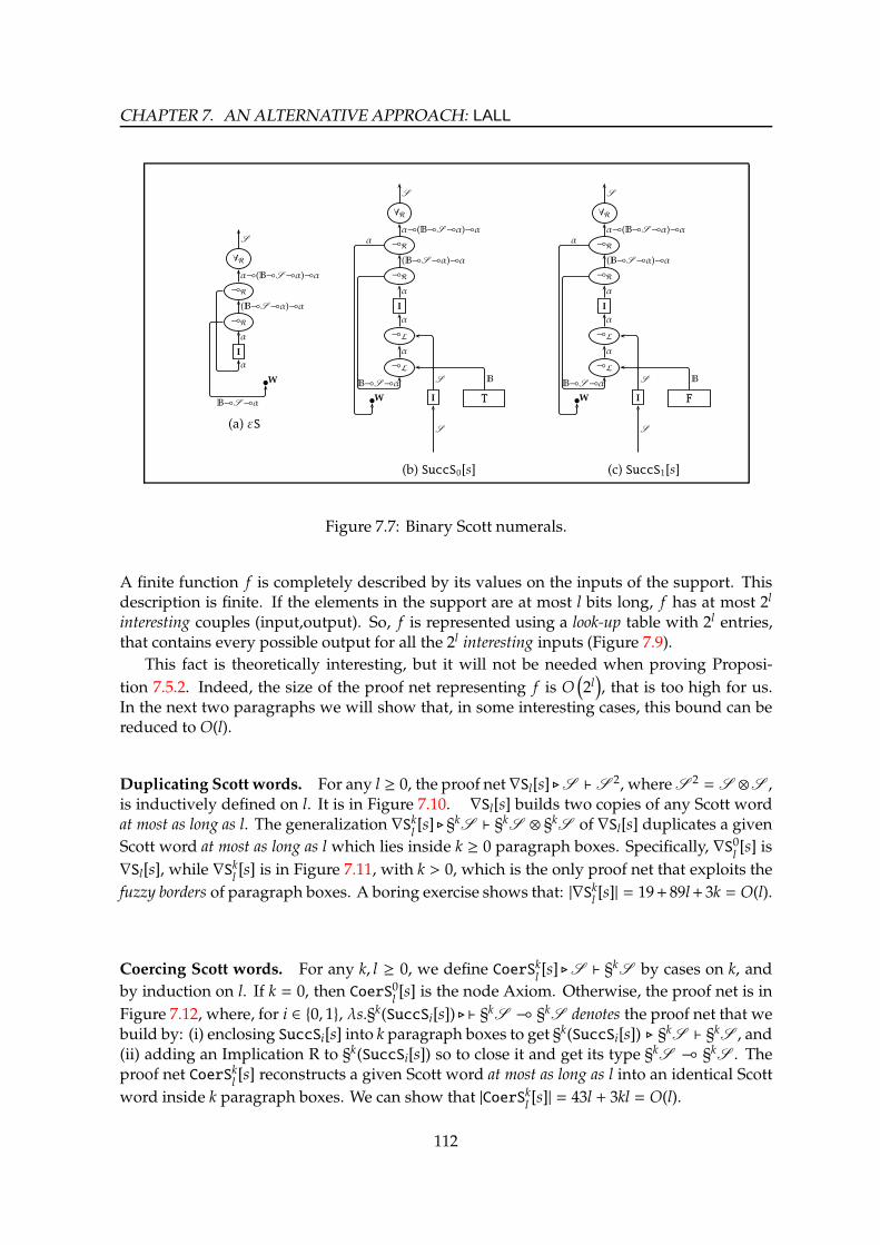
CHAPTER 7. AN ALTERNATIVE APPROACH: LALL
∀R
⊸R
⊸R
I
W
S
α⊸(B⊸S⊸α)⊸α
(B⊸S⊸α)⊸α
α
α
B⊸S⊸α
(a) εS
∀R
⊸R
⊸R
I
⊸L
⊸L
W I T
S
α⊸(B⊸S⊸α)⊸α
(B⊸S⊸α)⊸α
α
α
α
α
B⊸S⊸α
S
S B
(b) SuccS0[s]
∀R
⊸R
⊸R
I
⊸L
⊸L
W I F
S
α⊸(B⊸S⊸α)⊸α
(B⊸S⊸α)⊸α
α
α
α
α
B⊸S⊸α
S
S B
(c) SuccS1[s]
Figure 7.7: Binary Scott numerals.
A finite function f is completely described by its values on the inputs of the support. Thisdescription is finite. If the elements in the support are at most l bits long, f has at most 2l
interesting couples (input,output). So, f is represented using a look-up table with 2l entries,that contains every possible output for all the 2l interesting inputs (Figure 7.9).
This fact is theoretically interesting, but it will not be needed when proving Proposi-
tion 7.5.2. Indeed, the size of the proof net representing f is O(2l), that is too high for us.
In the next two paragraphs we will show that, in some interesting cases, this bound can bereduced to O(l).
Duplicating Scott words. For any l ≥ 0, the proof net ∇Sl[s] ⊲S ⊢ S 2, whereS 2 = S ⊗S ,is inductively defined on l. It is in Figure 7.10. ∇Sl[s] builds two copies of any Scott wordat most as long as l. The generalization ∇Sk
l[s] ⊲ §kS ⊢ §kS ⊗ §kS of ∇Sl[s] duplicates a given
Scott word at most as long as l which lies inside k ≥ 0 paragraph boxes. Specifically, ∇S0l[s] is
∇Sl[s], while ∇Skl[s] is in Figure 7.11, with k > 0, which is the only proof net that exploits the
fuzzy borders of paragraph boxes. A boring exercise shows that: |∇Skl[s]| = 19+89l+3k = O(l).
Coercing Scott words. For any k, l ≥ 0, we define CoerSkl[s] ⊲S ⊢ §kS by cases on k, and
by induction on l. If k = 0, then CoerS0l[s] is the node Axiom. Otherwise, the proof net is in
Figure 7.12, where, for i ∈ 0, 1, λs.§k(SuccSi[s]) ⊲ ⊢ §kS ⊸ §kS denotes the proof net that webuild by: (i) enclosing SuccSi[s] into k paragraph boxes to get §k(SuccSi[s]) ⊲ §kS ⊢ §kS , and(ii) adding an Implication R to §k(SuccSi[s]) so to close it and get its type §kS ⊸ §kS . Theproof net CoerSk
l[s] reconstructs a given Scott word at most as long as l into an identical Scott
word inside k paragraph boxes. We can show that |CoerSkl[s]| = 43l + 3kl = O(l).
112

7.4. PRELIMINARYUSEFUL PROOF NETS IN LALL
I
⊸L
⊸L ⊸R
ε ⊸R
∀L W I
S
S
S
S S
S
B⊸S⊸S
S⊸S
S
B
S
(a) predecessor.
⊸R
⊸R
⊸R
⊸R
I
⊸L
⊸L ⊸R
I ⊸R
W I
∀L ⊸L
⊸L
∀L
S⊸S⊸S⊸S⊸S
S
S
S
S S
S
B⊸S⊸S
S
S
S
S
S
S
S
BS
S
B
(b) conditional.
Figure 7.8: Basic operations over binary Scott numerals.
Scott words to words. The proof net StoCl[s] normalizes to the word w, for any Scott wordat most as long as l. We do not describe it, as it has a structure analogous to the proof netCoerS0
l[s] in Figure 7.12.
Lifting. Let Π ⊲ ~S n, ~§kSs⊢ §kS for some n, s, k ≥ 0. For every k′ ≥ 0 we can build
Lift[Π] ⊲ ~S n, ~§k+k′Ss⊢ §k+k
′S by: (i) enclosing Π into k′ paragraph boxes, gettingΠ′, and
(ii) plugging the conclusion of CoerSk′
l[s], using Cut, into every of the n premises with type
§k′S ofΠ′. The final proof net is in Figure 7.13. The proof net Lift[Π] isΠ deepened inside
k′ paragraph boxes. Notice that | Lift[Π]| = |Π| + k′(n + s + 1) + n|CoerSk′
l[s]| = O (|Π| + l).
Contracting the premises of a proof net. Let Π ⊲ ~A, §kS , §kS , ~A′ ⊢ A for some l, k ≥ 0.
We can build ∇kl[Π] ⊲ ~A, §kS , ~A′ ⊢ A by: (i) writing Π′ which is Π with a new Tensor
L between the two outlined premises of type §kS , and (ii) plugging the conclusion of∇Sk
l[s] ⊲ §kS ⊢ §kS ⊗ §kS , by a Cut, into the premise of the new Tensor L inΠ′. Notice that
|∇kl[Π]| = |Π| + |∇Sk
l[s]| + 2 = O(l).
113
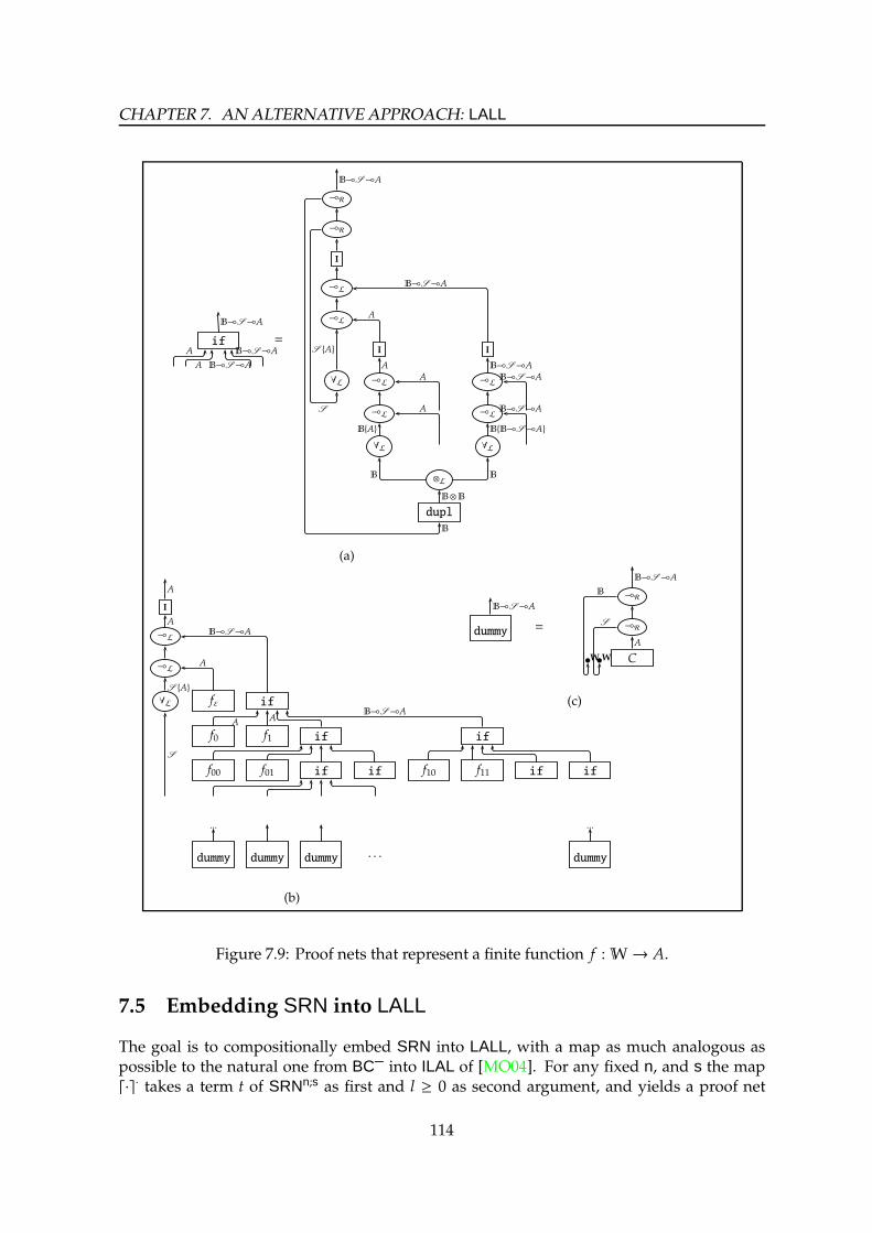
CHAPTER 7. AN ALTERNATIVE APPROACH: LALL
if =
B⊸S⊸A
A
A B⊸S⊸A
B⊸S⊸A
⊸R
⊸R
I
⊸L
⊸L
I I
∀L ⊸L ⊸L
⊸L ⊸L
∀L ∀L
⊗L
dupl
B⊸S⊸A
S A
S
B
A
A
BA
A
A
B⊸S⊸A
B⊸S⊸A
BB⊸S⊸A
B⊸S⊸A
B⊸S⊸A
B B
B⊗B
(a)
I
⊸L
⊸L
∀L fε if
f0 f1 if if
f00 f01 if if f10 f11 if if
... ...
dummy dummy dummy . . . dummy
A
A
A
S A
S
B⊸S⊸A
AAB⊸S⊸A
(b)
dummy =
B⊸S⊸A⊸R
⊸R
WW C
B⊸S⊸A
A
B
S
(c)
Figure 7.9: Proof nets that represent a finite function f :W→ A.
7.5 Embedding SRN into LALL
The goal is to compositionally embed SRN into LALL, with a map as much analogous aspossible to the natural one from BC– into ILAL of [MO04]. For any fixed n, and s the map⌈·⌉· takes a term t of SRNn;s as first and l ≥ 0 as second argument, and yields a proof net
114

7.5. EMBEDDING SRN INTO LALL
I
⊸L
⊸R
⊸L ⊸R
ε ⊗ ε I
∀L ⊸L
∇SM−1
⊸L
⊸L
∀L ⊸R ⊸R
⊗R ⊗R
succ0 succ0 succ1 succ1
⊗L ⊗L
⊸L ⊸L
S ⊗S
S ⊗S
S S ⊗S
S
B⊸S⊸S⊗S
S ⊗S
BS ⊗S⊸S⊗S
S ⊗S
B
S
S⊗S⊸S⊗S
S S
S⊗S⊸S⊗S
S S
(a) M > 0
ε ⊗ ε
W
S
S ⊗S
(b) M = 0:dummy value
Figure 7.10: The Duplication proof net ∇SM : S ⊸ S ⊗S .
⊗R
§k §k
Cut I I
∇Sl ⊗L
§k
(§kS )2= §kS ⊗§kS
§kS §kS
S S
S 2
S
§kS
Figure 7.11: The generalized duplication ∇Skl[s] of Scott words.
⌈t⌉l ⊲−→S
n,−−−→§kS
s⊢ §kS , for some k. We define the map inductively on the first argument.
115

CHAPTER 7. AN ALTERNATIVE APPROACH: LALL
⊸L ⊸R
⊸R
⊸L
⊸L
⊸L §k ⊸L
∀L εS ∀L λs.§k(SuccS0[s]) λs.§k(SuccS1[s]) CoerSkl−1
[s]
§kS
(B⊸S⊸§kS )⊸§kS
S §kS
S
§kS
B⊸S⊸§kS
§kS
B
§kS⊸§kS
§kS⊸§kS
§kS
Figure 7.12: The coerce proof net CoerSkl[s] on Scott words.
§k′
Π
§k′
§k′
§k′
§k′
CoerSk′
lCoerSk
′
l
. . . . . .
§kS
S
S §kS
§kS
§k+k′S
§k′S §k
′S
S S
§k+k′S §k+k
′S
Figure 7.13: The Lifting of a proof net Π representing f up toMwith k paragraphs.
The base cases of ⌈·⌉·. Some of them are straightforward:
⌈0⌉l = εS ⊲ ⊢ S ⌈si⌉l = SuccSi[s] ⊲ S ⊢ S (i ∈ 0, 1)
⌈P⌉l = PredS[s] ⊲ S ⊢ S ⌈B⌉l = CondS[s, x, y] ⊲ S ,S ,S ⊢ S
where, s, x, y jute denote the inputs of the proof nets they appear into. Concerning theprojection, ⌈πn;s
i⌉l is an Axiom that connects the i-th input to the conclusion, erasing all the
other inputs by Weakenings. An example with 1 ≤ i ≤ n is:
W . . . I . . . W W . . . W
S
SS S S S
Notice that k = 0 here.
The case of ⌈·⌉· on the composition. We now focus on t = [t′, u1, . . . , un, v1, . . . , vs] suchthat t′ be in SRNm;r. Because of space constraints, but without loss of generality, we show
how to build ⌈t⌉l by assuming m = n = s = 1, and r = 2. By induction we have:
⌈t′⌉obl(t) ⊲ S , §k′
S , §k′
S ⊢ §k′
S ⌈u1⌉l ⊲ S ⊢ §kuS
⌈vi⌉l ⊲ S , §kiS ⊢ §kiS (i ∈ 1, 2)
By letting k = maxk′, ku, k1, k2, we get:
116

7.5. EMBEDDING SRN INTO LALL
§m
Lift [⌈t′⌉obl(t)]
§m Cut Cut
Cut Lift [⌈v1⌉l] Lift[⌈v2⌉
l]
Lift[⌈u1⌉l] §m §m §m §m
coerce coerce
§2mW
§mW
W
§mW
§mW
W
§mW
W §mW
§mW
§2mW
W
§mW
W §mW
§mW
W
§2mW
Figure 7.14: The (partial) translation of [t′, u1, v1, v2] with missing contractions.
Lift[⌈t′⌉obl(t)] ⊲ S , §kS , §kS ⊢ §kS Lift[⌈u1⌉l] ⊲ S ⊢ §kS
Lift[⌈vi⌉l] ⊲ S , §kS ⊢ §kS (i ∈ 1, 2)
Next, if we buildΠ′ in Figure 7.14, then ⌈t⌉l is ∇2kl[∇0
l[∇0
l[Π′]]]. The two occurrences of ∇0
l
contract three “normal” premises. One is from ⌈u1⌉l. The other two are from ⌈v1⌉
l, ⌈v2⌉l. Theoccurrence of ∇2k
lcontracts the single “safe” premise of ⌈v1⌉
l and ⌈v2⌉l. We insist remarking
the existence of ⌈t⌉l for anym, n, r, s. One can count: |⌈t⌉l| ≤ | Lift[⌈t′⌉obl(t)]|+∑m
i | Lift[⌈ui⌉l]|+∑r
j | Lift[⌈u j⌉l]|+k(1+n+s′n+s′s)+s′n|CoerSk
l[s]|. So |⌈t⌉l| = O
(|⌈t′⌉obl(t)| +
∑mi |⌈ui⌉
l| +∑r
j |⌈v j⌉l| + obl(t)
).
The case of ⌈·⌉· on the recursion. Let t = r[uε, u0, u1] with uε ∈ SRNn;s, u0, u1 ∈ SRNn+1;s+1.Again, because of space constraints, we set n = s = 1 which is general enough to show the
key point of the embedding. In the course of the iteration unfolding that ⌈t⌉l carries out, thesafe argument gets duplicated, so we must contract them. By induction:
⌈uε⌉l ⊲ S , §kεS ⊢ §kεS ⌈ui⌉
obt(l) ⊲ S ,S , §kiS , §kiS ⊢ §kiS (i ∈ 0, 1)
By letting k = maxkε, k0, k1, and using Lift[·] in analogy to the translation of the com-position, ⌈t⌉l is in Figure 7.15. The first argument, i.e. the Scott word that drives the recursionunfolding, becomes a word, and, then, it is necessary to reverse it by RevC. Otherwise wewould unfold the iteration according to a wrong bit order, as implied by Remark 7.4.1. More-over, (i) Π projects the rightmost n + s + 1-th element of type A it gets in input and whichcontains the result, (ii) The two proof nets ⊗R , ⊗L are two obvious trees of Tensor R and
L nodes. Calculating the size, we get |⌈t⌉l| = O(|⌈uε⌉
l| + |⌈u0⌉obt(l)| + |⌈u1⌉
obt(l)| + obt(l)).
D 7.5.1 (S T P ) Let t be in SRNn;s, l ∈N, and Π ⊲ ~S n
~(§kS )s⊢ §kS , for some k ∈N. Then,Π k-simulates twith l-bounded inputs if, for every pair
of vectors of natural numbers ~xn, ~ys, such that |~xn|, |~ys| ≤ l, the proof net we get by plugging⌈x1⌉
l, . . . , ⌈xn⌉l, §k⌈y1⌉l, . . . , §k⌈ys⌉
l into the inputs ofΠ, in the natural way, normalizes to §k⌈z⌉l,whenever z is the result of t(~xn; ~ys).
P 7.5.2 (LALL SRN)Let l ≥ 0, and t ∈ SRNn;s. Then, ⌈t⌉l k-simulates t with l-bounded input. Moreover, (i)k ≤ ∂R(t) · 2∂C(t), and (ii) for every fixed t, |⌈t⌉l| is O (nbt(l)).
117
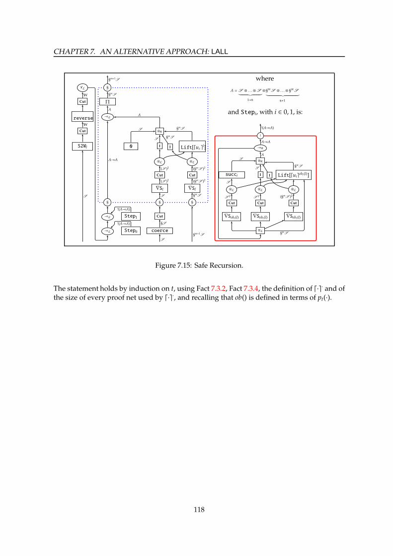
CHAPTER 7. AN ALTERNATIVE APPROACH: LALL
∀L §
Cut Π
reverse ⊸L
Cut ⊗R
S2Wl 0 I Lift[⌈uε⌉l]
⊗L ⊗L
Cut Cut
∇Sl ∇Sl
§ § §
⊸L Step1 Cut
⊸L Step0 coerce
§m+1S
§mS
A
A⊸A
A
S §mS
S §mS
(S )2
(S )2
S
(§mS )2
(§mS )2
I
§mS
S
§S
§m+1S
W
W
S
!(A⊸A)
!(A⊸A)
where
A =S ⊗ . . . ⊗S︸ ︷︷ ︸
1+n
⊗§mS ⊗ . . . ⊗ §mS
︸ ︷︷ ︸s+1
and Stepi, with i ∈ 0, 1, is:
!
⊸R
⊗R
succi I Lift[⌈ui⌉obt(l)]
⊗L ⊗L ⊗L
Cut Cut Cut
∇Sobt(l) ∇Sobt(l) ∇Sobt(l)
⊗L
!(A⊸A)
A⊸A
AS
S 2
S
S 2
S
(§mS )2
I
§mS
§mS
Figure 7.15: Safe Recursion.
The statement holds by induction on t, using Fact 7.3.2, Fact 7.3.4, the definition of ⌈·⌉· and ofthe size of every proof net used by ⌈·⌉·, and recalling that ob() is defined in terms of pt(·).
118

Chapter 8
Further directions
This last Chapter considers some possible directions for the future research. We have alreadybegun the exploration of some of these directions; some others, on the contrary, are just ideasfor future work.
First of all, in Section 8.1 we consider some subsystems that may possibly encode somemore functions of SRN than the ones that soLAL can represent. Two of them, co-soLAL andsoLAL∞, are natural extensions of soLAL. The third one is IEAL, Intuitionistic ElementaryAffine Logic, that is known to be not polytime. We conjecture anyway that it could bepolytime, under some reduction strategy.
In Section 8.2 we consider some possible generalizations of the framework MS. MS lacksseveral of the rules that one can find in literature. As we already said, we were interestedonly in stratified logics, because they are easier to handle than the other ones, and because oftheir philosophical similarity with tiering. We show that it is possible to extend MS withoutlosing stratification. MS+ is the extension of MSwith generalized contractions, i.e. contractionswith an arbitrary number of premises, on the style of [BM10, Laf04]. Then, MS† extends MSby the use of the levels of [BM10]. At last we shall consider untyped proof nets, and we shallallow some recursive types on the labels, as [BM07]. The reason for all these generalizationsis twofold. On one side, this potentially allows to capture inside MS other characterizationsof FPTIME different from ILAL: for example, L4 [BM10]. On the other side, as we said, MSrevealed not as expressive as we wanted: we were not able to encode all the SRN programsinside any subsystem of MS. So, maybe, a generalized subsystem of MS could be used forthis purpose. In Chapter 7 we have seen that this sometimes is true: the system LALL isnot a subsystem of MS, but it is a generalized subsystem, and it has revealed useful for ourresearch. LALL simulates all the SRN programs.
8.1 Beyond soLAL
As we pointed out, soLAL strictly extends ILAL, but we can’t embed the whole SRN intosoLAL. Here we propose two variation co-soLAL and soLAL∞ of soLAL that strictly extendsoLAL, and that could attain the target. IEAL will be considered in Section 8.1.3.
119

CHAPTER 8. FURTHER DIRECTIONS
8.1.1 co-soLAL
co-soLAL is the extension of soLAL with level-coercions, i.e. axioms extraneous to MS thatprove j§A⊸ i§A for every i < j. Essentially, these nodes make all the modalities equivalent,so that co-soLAL is not stronglypolytime; it is as expressive as IEAL (Intuitionistic ElementaryAffine Logic). “Equivalent” here is used with a technical meaning: the modalities are allequivalent under R↑. On the other side it is easy to encode SRN into co-soLAL. We showthat there exists a polytime reduction strategy, but using it not all the SRN programs reduce.So, at the moment, co-soLAL does not reach the prefixed target. Anyway, we conjecture thatsome strategy exists such that co-soLAL is polytime and all the SRN programs can reduce.
D 8.1.1 (co-soLAL) co-soLAL is the system soLALplus the LCnodes ( level-coercions)for every i < j:
LC
i§A
j§A
Notice that co-soLAL is not a subsystem of MS, because of the presence of the external nodesLC.
L 8.1.2 (A E M)In co-soLAL, for every pair of modalities (m, n), where n , 1!, it is possible to prove ⊢ mα ⊸nα, using the “Flat” proof nets in Figure 8.1. On the other hand, it is not possible to provemα⊸ 1!α, for any modality m , 1!.
L 8.1.3 (co-soLAL N S P)There exists a proof net in co-soLAL that takes an integer n and calculates 2n. Such a proofnet is in Figure 8.1.
Nevertheless, the system co-soLAL is polynomial-time in the following, weaker, sense.
D 8.1.4 (F S) A reduction Π → Σ is fast if the ns [Y/P] is applied onlywhen the box does not contain any LC node.
L 8.1.5 (W P co-soLAL)There exists a family of polynomials p∂,L(x) | ∂, L ∈ N such that for every proof net Π of co-soLAL, whose depth is at most ∂, contains at most L LC nodes, and for every fast reductionΠ→k Σ, p∂,L(|Π|) bounds both k and |Σ|.
Proof. LetΠ be as in the hypothesis, and b be a fixed box at depth d inΠ. We want to show abound on the number of consecutive spindles inΠ, so we will able to adapt Lemma 4.3.31 tothis situation. Let us consider a chain ofN consecutive spindles. The spindles are connectedthrough modal formulas i1!A1, . . . , in−1!An−1 whose sorts i j strictly increase, unless some LCbox is present. Without LC’s, at mostM consecutive spindlesmay exist. Each LC let to add atmostM new spindles to the chain; soM ·L is a bound for the number of consecutive spindles.Now, thanks to (the proof of) Lemma 4.3.31, for each box b it holds RΠ(b) ≤ |Π|
M·L+1. Duringthe reduction, L does not increase because we are using the fast strategy. Now, we can look
120

8.1. BEYOND SOLAL
!
LC
§
k!A
k§A
i§A i<k
j!A i< j
!
LC
k§A
i§A
k!A i<k
(a) Some of the Flat proof nets
o
⊸R
Po
⊸L
2
Pi
⊸L
∀L Po
⊸R
Flat
Po
add
Pi Pi
Y
N⊸ j§k!N
j§k!N
k!N
k!N
j§(k!N⊸k!N)
N
j!(k!N⊸k!N)
k!N⊸k!N
k!N
k§N
N
N N
k!N k!N
(b) The exponential proof net, with k ≥ 2
Figure 8.1: This proofnet, in co-soLAL, if reduced, reduces in exponential time. It corresponds
to the λ-term λn.(λy.add yy)2. The integers areN = ∀α. j!(α⊸ α)⊸ j§(α⊸ α) for some j.
back at the proof of Lemma 4.3.24 and we understand that it still holds: our bound on RΠimplies a bound on the normalization time and size. 2
Notice that we cannot deduce that P is polynomial time, according to Definition 4.1.4,but just that there is a polynomial that bounds the reduction as described in the statement ofthis Lemma.
The fast reduction is not enough to represent SRN in co-soLAL. Indeed, let us think againto the recursive scheme. It takes a function g : jW⊸ ( jWn)⊸ ( jW)s ⊸ jW, encloses it in abox, duplicates it as many times as needed, and at last applies the functions to the argument.
Then, the recursion scheme returns a function f : jW ⊸ ( jWn)⊸(i§3 j§ jW
)s⊸ i§4 jW; it is
necessary at least one LC node to transform it to the right type f ′ : jW⊸ ( jWn)⊸ ( jW)s ⊸jW. To iterate f ′, we put it inside a box, thus we would need to duplicate a box containingan LC node, and the fast strategy does not allow this.
121
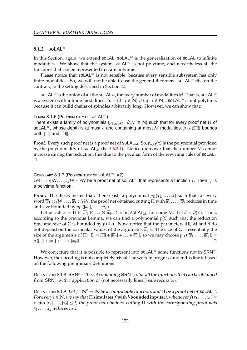
CHAPTER 8. FURTHER DIRECTIONS
8.1.2 soLAL∞
In this Section, again, we extend soLAL. soLAL∞ is the generalization of soLAL to infinitemodalities. We show that the system soLAL∞ is not polytime, and nevertheless all thefunctions that can be represented in it are polytime.
Please notice that soLAL∞ is not sensible, because every sensible subsystem has onlyfinite modalities. So, we will not be able to use the general theorems. soLAL∞ fits, on thecontrary, in the setting described in Section 4.5.
soLAL∞ is the union of all the soLALM, for everynumber ofmodalitiesM. That is, soLAL∞
is a system with infinite modalities: X = i! | i ∈ N ∪ i§ | i ∈ N. soLAL∞ is not polytime,because it can build chains of spindles arbitrarily long. However, we can show that:
L 8.1.6 (P soLAL∞)There exists a family of polynomials p∂,M(x) | ∂,M ∈ N such that for every proof net Π ofsoLAL∞, whose depth is at most ∂ and containing at most M modalities, p∂,M(|Π|) boundsboth [Π] and ‖Π‖.
Proof. Every such proof net is a proof net of soLALM. So, p∂,M(x) is the polynomial providedby the polynomiality of soLALM (Fact 6.2.1). Notice moreover that the number M cannotincrease during the reduction, this due to the peculiar form of the rewriting rules of soLAL.2
C 8.1.7 (P soLAL∞, #2)Let Π : i1W, . . . , ikW ⊢ jW be a proof net of soLAL∞ that represents a function f . Then, f isa polytime function.
Proof. The thesis means that: there exists a polynomial pΠ(x1, . . . , xk) such that for everywordw1 : i1W, . . . ,wk : i1W, the proof net obtained cuttingΠwith w1, . . . ,wk reduces in timeand size bounded by pΠ (|w1|, . . . , |wk|).
Let us call Σ = Π 1 w1 1 . . . 1 wk. Σ is in soLALM, for some M. Let d = ∂(Σ). Thus,according to the previous Lemma, we can find a polynomial p(x) such that the reductiontime and size of Σ is bounded by p (|Σ|). Now, notice that the parameters |Π|, M and d donot depend on the particular values of the arguments wi’s. The size of Σ is essentially thesize of the arguments of Π: |Σ| = |Π| + |w1| + . . . + |wk|, so we may choose pΠ (|w1|, . . . , |wk|) =p (|Π| + |w1| + . . . + |wk|). 2
We conjecture that it is possible to represent into soLAL∞ some functions not in SRN–.However, the encoding is not completely trivial.The work in progress under this line is basedon the following preliminary definitions:
D 8.1.8 SRN± is the set containing SRN–, plus all the functions that can be obtainedfrom SRN– with 1 application of (not necessarily linear) safe recursion.
D 8.1.9 Let f :Nk →N be a computable function, andΠ be a proof net of soLAL∞.For every l ∈N, we say that Π simulates f with l-bounded inputs if, whenever f (x1, . . . , xk) =x and |x1|, . . . , |xk| ≤ l, the proof net obtained cutting Π with the corresponding proof netsx1, . . . , xk reduces to x.
122

8.1. BEYOND SOLAL
Then, our conjecture is:
C 8.1.10 (soLAL∞ SRN± l- ) There exists a composi-tional map ⌈·⌉· that translates every SRN± program f (~x; ~y) into a proof net ⌈ f (~x; ~y)⌉l of soLAL∞,such that ⌈ f (~x; ~y)⌉l represents f (~x; ~y) with l-bounded inputs.
Proof idea. Let us imagine we want implement a proof net Π calculating the recursivefunction starting from functions g, h0, h1 ∈ SRN–. Instead of really implementing a recursion,we just implement a composition of a sufficient number of copies of the step functions h0, h1.The greater is l, the greater is the tier of the output ofΠ; so it is necessary to work in soLAL∞,and not just insoLAL. 2
8.1.3 IEAL
We have already pointed out (page 89) that IEAL is a non-polytime subsystem of MS. Herewe describe how to map every SRN program into IEAL in a compositional way. Of course,this is not very interesting because IEAL is not polytime; anyway, we hope that some dayIEAL will be proved weakly polytime, under some reduction strategy σ that we don’t knowyet.
The most natural translation is an adaptation of the Murawski-Ong coding for ILAL.f (~x; ~y) is mapped into Π :W, . . . ,W, !mW, . . . , !mW ⊢ !mW, withW = !(α ⊸ α)⊸ !(α⊸ α)and for some m ≥ 0. Of course all the functions in BC– can be encoded in this way; but,this time, it is possible to contract the safe variables, thus getting full SRN. The number k isconnected to the number of safe recursions used to build f .
This result is not interesting, not only because IEAL is elementary-time, but because it ispossible to represent in IEAL some elementary functions. Nevertheless, notice that some ofthe restrictions on the safe/normal variables typical of SRN still hold in IEAL. For example,IEAL provesW⊸ !W but !W 6⊸W.
Now, the real problem lies in juxtaposition: in IEAL it can be encoded as concat :W ⊸ W ⊸ W, that is with only safe variables. As we said in Section 2.9, this allows theconstruction of some non-polytime function. So, the unknown strategy σ that we mentionedbefore, necessarily must not reduce such a proof net concat.
Another related observation.
P 8.1.11Let P ⊆ MS be a subsystem that enjoys the strong normalization property. Let us supposethat P is weakly polytime. Then, for every Π ∈ PN(P), |nf(Π)| is polynomial in |Π|.
Proof. Almost immediate. By hypotheses there is a normalization strategy σ such that Πreduces to nf(Π) in polynomial time and polynomial size. So, nf(Π) has polynomial size. 2
The latter Proposition is quite naıve, and nevertheless captures a behaviour that is quiteuncommon in the practice of subsystems of MS: firstly, there exists a normal form; secondly,the size of nf(Π) is polynomial, independently on the chosen (possibly elementary-time)normalization strategy. This is exactly the behaviour of SRN.
123

CHAPTER 8. FURTHER DIRECTIONS
8.2 Generalizations
Let us return to the original problem: embedding SRN into some stratified logic. Insteadof going on about soLAL, we could imagine several different light logic for this purpose. Inparticular, we can imagine to extend the framework MS with several different constructions,without giving up to the stratification.
8.2.1 Generalized Contractions
The multiplexor of [Laf04], as well as the contraction of [BM10], have an arbitrary number ofpremises. Let us consider a contraction with n ≥ 1 conclusions:
. . .
Y n ≥ 1
!qA
m1Am2A mnA
We denote Yq(m1, . . . ,mn) such a rule. n is called the rank of the contraction. The rank rk(Π)of a proof net Π is the maximum of the ranks of its contractions; and we will call rkd(Π),for d ≤ ∂(Π), the maximum of the ranks of the contractions at depth d. MS+ ⊇ MS is theframework including all these new rules. We want to show that all the theorems for MS stillhold in MS+.
L 8.2.1 (G C 4.3.25)Let P ⊆ MS+. Let us assume there exists a polynomial r(x) such that for every proof net Πof P and for every d Wd(Π) ≤ r (|Π|). Then P is strongly polytime.
Proof. The proof is long, but similar to the one of Corollary 4.3.25. The only difference is thedefinition of the modified weight Td (defined on page 55):
Td(Π) =∑
u∈VdΠ
Td(Π, u)
Td(Π, u)def=
1 u ∈ I, cut,W,h,Pi(m), i, o
3 u ∈ ⊗L,⊗R,∀L,∀R,⊸L,⊸R,Yq(m, n)
3 · (PΠ(u) + 1) ·∑τ∈O(b) len(τ) u ∈ Po(m).
Notice that the only difference is the case for Po(m). The modification is due to the [P/Y]reduction rule: here, we do not know a priori the number of premises of the contraction, soa more complicated expression is needed. The new expression involves the length len(τ) ofthe paths starting from the Po node, exactly as in [DL08]. 2
L 8.2.2 (G L 4.3.31: S C N P)Let P ⊆ MS+. Let us assume that every chain of spindles that can be built in P cannot havemore than L spindles, for some constant L ∈ N. Then there exists a polynomial p(x) suchthat for every Π ∈ PN(P), for every d ≤ ∂(Π) and for every b ∈ Bd
Π,
RΠ(b) ≤ p (|Π|d).
124

8.2. GENERALIZATIONS
Proof. Let us fix a box b at depth d; we want to count how many copies of d will becreated during the reduction. We call n = rkd(Π). Then, we can proceed as in the proof ofLemma 4.3.31 at page 61: we divide the nodes ofΠ at depth d in (at most) L+1 classes (we donotwrite again the classification, because it can be found in the cited proof). Πi is the module(modules were defined at page 32) containing all the nodes of class at most i, and mi is thenumber of (generalized) contractions of class-i. Ri is the number of paths starting from b andmaximal relatively to Πi, so that RΠ(b) = RL. Every contraction may split a path into at mostn new paths, so
R0 ≤ (n − 1) ·m0 + 1
Ri+1 ≤ Ri · ((n − 1) ·mi + 1)
RΠ(b) = RL ≤
L∏
j=0
((n − 1) ·mi + 1) ≤ nL+1 · |Π|dL+1 ≤ |Π|d
2(L+1).
2
P 8.2.3 (G P 4.3.40: A P C)Let P ⊆ MS+ sensible. The following are equivalent:1. P is polytime.2. P cannot build any dangerous spindle.
Proof. 2.⇒ 1. Follows from Lemma 8.2.2. 1.⇒ 2. The presence of a dangerous spindle leadsto the construction of a family of proof nets that reduces in exponential time, exactly as inLemma 4.3.39. 2
T 8.2.4 (G T 4.4.25: S M S S)Let P ⊆ MS+ be a sensible subsystem with a linear and with modalities in X. P is maximaliff P contains exactly the following rules:1. all the rules Yq(m, n) for every choice of q ≺ m, n in X;2. all the rules Yq(q, n) for every choice of q ≺ n in X;3. all the rules Pq(q
?,m∗1, . . . ,m∗
k) for every choice of m1, . . . ,mk ≺ q in X;
4. only one among Yq(q, q) and Pq(q∗,m∗
1, . . . ,m∗
k), for every m1 . . . ,mk ≺ q in X.
The proof is analogous to the one of Theorem 4.4.25.
8.2.2 Levels
The systemLight Linear Logic byLevels,orL4, of [BM10] is an extension of ILAL characterizedby the notion of levels and indexings. Intuitively, the systemallows some rules that, apparently,seem some derelictions:
Γ,A ⊢ BΓ, §A ⊢ B
§ Γ ⊢ BΓ, !A ⊢ B
!
However, inside a proof, each occurrence of such rules must be in some way balanced withother occurrences, thus forming some levels inside the proof net; as a consequence each groupof such rules appear more similar to a promotion than to a dereliction. L4 allows only suchbalanced proofs. The formal definition of proof net of L4 relies on the notion of indexing, aproof net being accepted if and only if it allows an indexing.
125

CHAPTER 8. FURTHER DIRECTIONS
Here we will extend MS with levels. The new framework is called MS†. There will betwo different kinds of boxes: some ones will be physical, with a clear border, and containinga proof net inside them; the other ones will be fuzzy, their border will not be drawn andthey can contain a graph that is not necessarily a proof net. A fuzzy box can also have moreconclusions! Just to help the readability, sometimes we will draw these fuzzy boxes, with adashed line. However, we consider only a very simplified situation: there will be no wayto duplicate the content of a fuzzy box. This is what happens, e.g., in L4: the !-boxes arephysical and can be duplicated, while the §-boxes are fuzzy and cannot be duplicated. Thispropertywill be assured by the presence of twodisjoint setsX,Y ofmodalities: themodalitiesbelonging to Xwill behaves differently from the modalities in Y.
We find quite difficult to handle levels. The only result of this Section is a sufficientcondition for polytime soundness (Proposition 8.2.21). To prove it, it will be necessary thewhole power of the CS as it appears in [DL08]. We now try to give an intuition of whyour CS is not sufficient. The subsystems that use indexings are not really stratified, but justweakly stratified. For example, a normal box can intersect with a fuzzy box. In this case, itcan still happen that a CS-path enters into one of such boxes; but the point is, where shouldit continue? after the solid box, or after the fuzzy box? or none? The only way to manage thesituation is to consider all the possible CS-paths provided by the standard CS, and not onlyour CS-paths.
Formally, let us fix two sets of modalities X and Y disjoint. We are going to define thequasi-proof nets: only some of them will be called proof nets. The quasi-proof nets of MS†X,Yare defined by induction using all the linear and affine cases of Definition 3.1.3 at page 26,plus the following non linear cases:
Rule Pq(m1, . . . ,mk) or Promotion: If q ∈ X, and m1, . . . ,mk ∈ X∪Y, then the following is aproof net:
o
Po(q)
Π
Pi(m1) Pi(...) Pi(mk)
i i i
qC
C
A1 ... Ak
m1A1... mkAk
Rule Yp(m, n) or Contraction: If Ai = mA and A j = nA for some i, j, and moreover p ∈ X andm, n ∈ X∪Y, then the following is a proof net:
o
Π
i . . . . . . . . . i
Yp(n,m)
i
C
A1 Ar
mA nA
pA
126

8.2. GENERALIZATIONS
Po(m)
i
i+1
Pi(m)
i+1
i
i
i
Box Output Box Inputall the othernodes
Figure 8.2: Constraints for indexing proof structures.
Port right: Ifm ∈ Y, the following is a proof net:
o
Po(m)
Π
i i i
mC
C
A1 ... Ar
Port left: If m ∈ X∪Y, the following is a proof net:
o
Π
i . . . Pi(m) . . . i
i
C
A1
Ai
Ar
mAi
D 8.2.5 (I) Let Π be a quasi-proof net of MSX,Y. An indexing for Π is afunction I from the edges of Π to Z that satisfies the constraints in Figure 8.2 and such thatI(e) = I(e′), for every premise or conclusion e, e′ of Π. An indexing I is canonical if Π has anedge e such that I(e) = 0, and I(e′) ≥ 0 for all edges e′ of Π.
D 8.2.6 (P ) Let Π be a quasi-proof net. Π is a proof net of MSX,Y iff itadmits an indexing.
R 8.2.7 A box input is not a dereliction. The indexing forces every box input to bebalanced with some box output, so that in fact box inputs and outputs form a boundary for asubgraph that we can call a fuzzy box: a region with a fuzzy border.
As an example, L4 is a subsystem of MS†X,Y with X = ! and Y = §.
F 8.2.8 (R)If I is an indexing for Π and n ∈ Z, then also I′(e)
def= I(e) + n defines an indexing for Π.
F 8.2.9 (C I)Every proof net of MSX,Y has one and only one canonical indexing.
127
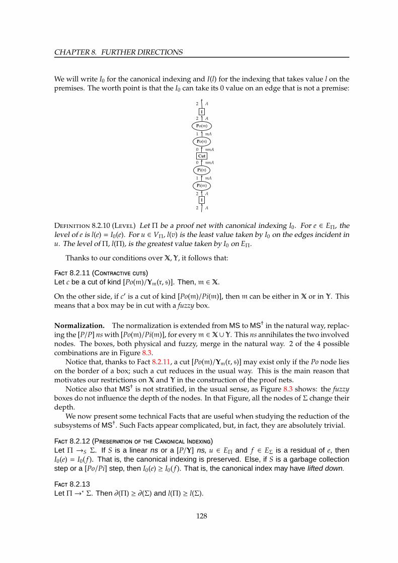
CHAPTER 8. FURTHER DIRECTIONS
We will write I0 for the canonical indexing and I(l) for the indexing that takes value l on thepremises. The worth point is that the I0 can take its 0 value on an edge that is not a premise:
I
Po(m)
Po(n)
Cut
Pi(n)
Pi(m)
I
2 A
2 A
1 mA
0 nmA
0 nmA
1 mA
2 A
2 A
D 8.2.10 (L) Let Π be a proof net with canonical indexing I0. For e ∈ EΠ, thelevel of e is l(e) = I0(e). For u ∈ VΠ, l(v) is the least value taken by I0 on the edges incident inu. The level of Π, l(Π), is the greatest value taken by I0 on EΠ.
Thanks to our conditions over X,Y, it follows that:
F 8.2.11 (C )Let c be a cut of kind [Po(m)/Ym(r, s)]. Then, m ∈ X.
On the other side, if c′ is a cut of kind [Po(m)/Pi(m)], then m can be either in X or in Y. Thismeans that a box may be in cut with a fuzzy box.
Normalization. The normalization is extended from MS to MS† in the natural way, replac-ing the [P/P] nswith [Po(m)/Pi(m)], for everym ∈ X∪Y. This ns annihilates the two involvednodes. The boxes, both physical and fuzzy, merge in the natural way. 2 of the 4 possiblecombinations are in Figure 8.3.
Notice that, thanks to Fact 8.2.11, a cut [Po(m)/Ym(r, s)] may exist only if the Po node lieson the border of a box; such a cut reduces in the usual way. This is the main reason thatmotivates our restrictions on X and Y in the construction of the proof nets.
Notice also that MS† is not stratified, in the usual sense, as Figure 8.3 shows: the fuzzyboxes do not influence the depth of the nodes. In that Figure, all the nodes of Σ change theirdepth.
We now present some technical Facts that are useful when studying the reduction of thesubsystems of MS†. Such Facts appear complicated, but, in fact, they are absolutely trivial.
F 8.2.12 (P C I)Let Π →S Σ. If S is a linear ns or a [P/Y] ns, u ∈ EΠ and f ∈ EΣ is a residual of e, thenI0(e) = I0( f ). That is, the canonical indexing is preserved. Else, if S is a garbage collectionstep or a [Po/Pi] step, then I0(e) ≥ I0( f ). That is, the canonical index may have lifted down.
F 8.2.13Let Π→∗ Σ. Then ∂(Π) ≥ ∂(Σ) and l(Π) ≥ l(Σ).
128

8.2. GENERALIZATIONS
Po(q)
Π
Pi(m)
Cut
Po(m)
Σ
Pi(n)
→
Po(q)
Π
Cut
Σ
Pi(n)
(a) [Po(m)/Pi(m)], with m ∈ Y, q ∈ X
Po(q)
Π
Pi(m)
Cut
Po(m)
Σ
Pi(n)
→
Po(q)
Π
Cut
Σ
Pi(n)
(b) [Po(m)/Pi(m)], with m ∈ X, q ∈ Y
Figure 8.3: Two of the 4 possible cases in the reduction [Po(m)/Pi(m)]. For clarity reasons, wehave drawn all the boxes with one only premise and one only conclusion.
F 8.2.14Let Π →S Σ. We consider the same indexing I(l) over Π and Σ. S is a ns involving a cut ofΠ at depth d and index i. If S = [Po/Y], then Σ can contain new cuts only at depth ≥ d. IfS = [Po/Pi], then Σ can contain new cuts only at level ≥ i. For every other S, Σ can containnew cuts only at depth d and level i.
Our notion of context semantics (Section 4.3.1) appears too weak to handle levels. Fromnow on, we will use the full power of context semantics of [DL08]. Context semanticsis generally used to study properties of strong polynomiality, i.e. independently from thereduction strategy. To simplify the work, on the contrary, we will require that gc steps arealways performed only when no other ns exist. These are the slowest possible reductions:every duplication is always performed, even if the reducts will eventually disappear due toa gc.
We now recall the CS as in [DL08]. An exponential signature is a formula generated bythe following grammar:
tdef= e | r(t) | l(t).
E is the set of exponential signatures. A stack element is an element of Sdef= a, o, f, s, x ∪ E,
for everym ∈ X∪Y. A stack is a finite non empty sequence of stack elements. LetΠ a proofnet. Then a context of Π is an element of
CΠdef= EΠ × E
∗ × S+ × B.
The rewriting relation among contexts C 7→Π C′ is described in Figure 8.4.
Particular kinds of stacks U ∈ S+ are the final stacks. We distinguish positive (denoted
129

CHAPTER 8. FURTHER DIRECTIONS
⊸R
he
g
(g,U,V,+) 7→Π (h,U,V · o,+)(e,U,V,−) 7→Π (h,U,V · a,+)(h,U,V · o,−) 7→Π (g,U,V,−)(h,U,V · a,−) 7→Π (e,U,V,+)
⊸L
h
eg
(g,U,V,+) 7→Π (e,U,V · a,−)(h,U,V,−) 7→Π (e,U,V · o,−)(e,U,V · a,+) 7→Π (g,U,V,−)(e,U,V · o,+) 7→Π (h,U,V,+)
⊗R
h
e g
(e,U,V,+) 7→Π (h,U,V · f,+)(g,U,V,+) 7→Π (h,U,V · x,+)(h,U,V · f,−) 7→Π (e,U,V,−)(h,U,V · x,−) 7→Π (g,U,V,−)
⊗L
e g
h
(h,U,V · f,+) 7→Π (e,U,V,+)(h,U,V · x,+) 7→Π (g,U,V,+)(e,U,V,−) 7→Π (h,U,V · f,−)(g,U,V,−) 7→Π (h,U,V · x,−)
∀R
g
e
(e,U,V,+) 7→Π (g,U,V · s,+)(g,U,V · s,−) 7→Π (e,U,V,−)
∀L
g
e
(e,U,V · s,+) 7→Π (g,U,V,+)(g,U,V,−) 7→Π (e,U,V · s,−)
Yc(a,b)
e g
h
(h,U,V · l(t),+) 7→Π (e,U,V · t,+)(h,U,V · r(t),+) 7→Π (g,U,V · t,+)(e,U,V · t,−) 7→Π (h,U,V · l(t),−)(g,U,V · t,−) 7→Π (h,U,V · r(t),−)
I
g
e
or Cut
g
e
(e,U,V,+) 7→Π (g,U,V,+)(g,U,V,−) 7→Π (e,U,V,−)
Po(m)
g
e
(e,U · e,V,+) 7→Π (g,U,V · e,+)(g,U,V · e,−) 7→Π (e,U · e,V,−)
Pi(m)
g
e
(e,U,V · e,+) 7→Π (g,U · e,V,+)(g,U · e,V,−) 7→Π (e,U,V · e,−)
Po(q)
Σ
Pi(m1) ...
. . .
h
l
gg
e
(e,U,V,+) 7→Π (h,U,V,+)(e,U,V · t,+) 7→Π (g,U · t,V,+)
(h,U,V,−) 7→Π (e,U,V,−)(g,U · t,V,−) 7→Π (e,U,V · t,−)
Figure 8.4: Rewriting Relation among contexts. Notice that if (e,U,V, b) 7→Π (e′,V′,U′, b′)then also (e′,U′,V′, b′ ↓) 7→Π (e,U,V, b ↓).
with P) and negative (denoted with N) final stacks and define them mutually recursively:
P : := e | P · e | P · o | P · f | P · x | P · s | N · a;
N : := N · t | N · o | N · f | N · x | N · s | P · a .
For example, the stack e · a · l(e) is negative final, while e · a · f · a is positive final. Acontext C ∈ CΠ is final iff one of the following four cases hold:
• If C = ((u, v),U,V,+), α(v) = o and V is a positive final stack;• If C = ((u, v),U,V,+), α(v) =W and V is a positive final stack;• If C = ((u, v),U,V,−), α(v) = i and V is a negative final stack.
A context is said canonical if |U| = l(e).
A CS-path overΠ ∈ PN(MSX,Y) is a sequence of canonical contexts connected throughthe rewriting relation. A CS-path is maximal if it begins from a Po and terminates in a finalcontext.
In Section 4.3.1 we defined theweightWd and themodified weight Td for each depth d; here,
130

8.2. GENERALIZATIONS
we cannot distinguish the various depths:
W(Π) =∑
b∈BΠ
RΠ(b) where
RΠ(b) = number of maximal CS-paths starting from b.
T(Π) =∑
u∈VΠ
TΠ(u) where
TΠ(u) =
1 α(u) < Po,Pi
0 α(u) = Pi
(PΠ(u) + 1)∑
t∈O(u) len t α(u) = Po
The following three Lemmas are essentially proved in [DL08].
L 8.2.15 (P MW)Let Π→ Σ. (a) T(Π) > T(Σ), so that [Π] ≤ T(Π). (b) |Π| ≤ T(Π), so that ‖Π‖ ≤ T(Π).
L 8.2.16 (P, R T, U S)Let Π → Σ. (a) W(Π) ≥ W(Σ). (b) There exists a polynomial p(x, y) such that T(Π) ≤p (W(Π), |Π|), so that also [Π], ‖Π‖ ≤ p (W(Π), |Π|). (c) W(Π) ≤ [Π] + ‖Π‖.
Letting ‖U‖ the number of exponential signatures in the stack U, we can prove that:
L 8.2.17 (S)Let Π ∈ PN(MSX,Y), and (e,U,V, b) 7→∗
Π(e′,U′,V′, b′). Then ‖U‖ + ‖V‖ = ‖U′‖ + ‖V′‖.
The Definition 4.3.26 of spindle, as well as the Definition 4.3.27 of chain of spindles areuntouched, just be careful that they now relies on a different definition of CS-paths:
D 8.2.18 (S D S) Let P ⊆ B†X,Y, Π ∈ PN(P); e ∈ EΠ anedge labelled mA entering a contraction u; f ∈ EΠ an edge labelled nB outgoing a Po nodeb; ∂(e) = ∂( f ). A spindle mA :Σ : nB between e and f (or also between u and b) is a pair ofCS-paths: τ from e to f passing through the left conclusion of u; ρ from e to f passing throughthe right conclusion of u; and such that τ and ρ are the only CS-paths connecting e with f .e, f , u are resp. the principal premise, principal conclusion and principal contraction ofΣ. An edge that is premise (resp. conclusion) of a node of Σ, but that is not part of Σ, is saidnon-principal premise (resp. conclusion). We shortenmA :Σ :nB with m :Σ :n. Finally, everymA :Σ :mB is dangerous.
D 8.2.19 (C S) LetP ⊆ BX,Π ∈ PN(P),Π containing r ≥ 1 spindlesmodm1A1 :Σ1 :n1B1, . . . ,mrAr :Σr :nrBr. Let us suppose that each spindle Σi is between nodesui and bi, and for each i < r Π contains a CS-path between bi and ui+1. The graph composedof the r spindles and the r − 1 CS-paths is called a chain of r spindles, and we shall writem1A1 :Θr :nrBr for it. |Θr| = r denotes the number of spindles it contain.
Finally, every mA :Θr :mB is dangerous.
Let P ⊆ MSX,Y. Let us assume there is a constant L ∈ N such that no more than Lconsecutive spindles may exist in a proof net Π ∈ PN(P). We say that P has determinacy
degree L. The strong determinacy of [DL08] is in fact a particular case: the determinacydegree is 1.
131

CHAPTER 8. FURTHER DIRECTIONS
L 8.2.20 (D)Let P ⊆ MS†X,Y with determinacy degree L ∈ N. Then, there exists a polynomial p(x) suchthat for every u ∈ VΠ, RΠ(u) ≤ p(|Π|). The degree of p(x) is L + 1.
Proof. This proof is analogous to the one of Lemma 4.3.31, this time classifying all thecontractions in Π instead of just contractions at level d.
Let b be a fixed box at depth d in Π.
1. Wewant to classify the links u ∈ VΠ in classes, class-0, class-1, class-2, . . . according to howmany consecutive spindles there are between b and u. Let us consider all the possible paths τbetween b and u. Let us call Σu
bthe module made up of all the nodes of all the τ’s. Let
us consider all the possible chains of spindles Φub,Ψu
b, . . . ,Ωu
bwhose nodes are among the
nodes of Σub. u is said class-i if i = max
∣∣∣Φub
∣∣∣ ,∣∣∣Ψu
b
∣∣∣ , . . . ,∣∣∣Ωu
b
∣∣∣. Notice that there are at most
L + 1 classes (0, . . . , L) by hypothesis.2. Let mi be the number of Contractions and Po nodes of class-i, and m = m0 + . . . + mL. We
observe that m ≤ |Π|.3. P will denote the greatest number of premises of the (non-fuzzy) boxes in Π, if this is
greater or equal than 2; otherwise, we state P = 2.4. For 0 ≤ i ≤ L, let Πi be the module containing all and only the class- j nodes, for every j ≤ i.5. A path τ starting from b ismaximal relatively toΠi if there exists a maximal path τ′ starting
from b whose intersection with Πi is exactly τ.6. We call Ri, for 0 ≤ i ≤ L, the number of paths starting from b and maximal relatively toΠi.
The definitions imply RΠ(b) = RL.
We prove that Ri ≤∏i
j=0
(P ·m j + 1
)by induction on i. Two paths separate only in a contrac-
tion node or in a (non-fuzzy) promotion box, but not in a ⊗L node, which, instead, forces togo in one specific direction. This time, differently from Lemma 4.3.31, we have to deal alsowith paths that arrive to a Po link with negative context, and also in that point the paths canseparate, in at most P different paths.
InΠ0 there are no spindles,meaningR0 ≤ m0+1. By induction, letRi−1 ≤∏i−1
j=0
(P ·m j + 1
).
Then, the paths maximal relatively toΠi are at most Ri ≤ Ri−1 · (P ·mi + 1) ≤∏i
j=0
(P ·m j + 1
).
So, RΠ(b) = RL ≤∏L
j=0(P ·mi + 1) ≤ (P · |Π|)L+1. 2
P 8.2.21 (D P S)Let P ⊆ MS†X,Y with determinacy degree L ∈N. Then, P is polytime.
Proof. Consequence of Lemma 8.2.20 and Lemma 8.2.16. 2
8.2.3 Untyped Proof nets, Recursive Types
Here we consider two classical generalizations of proof nets, related to each other. Bothsuch generalizations may lead to some new subsystems stratified, and nevertheless muchmore expressive than the actual subsystems of MS. This is why we are interested in a newframework allowing them. We shall see that it is reasonable to have MS proof nets withrecursive types; less reasonable to have untyped MS proof nets.
132

8.2. GENERALIZATIONS
Untyped proof nets. It is in the tradition of Light Logic that proof nets can be definedwith or without types, that is formulæ, labelling their edges. The results of polynomial timesoundness for LLL, ILAL, SLL, hold for all the proof nets, typed and untyped ones. Untypedproof nets, on the logical point of view, are wrong proofs; and anyway there are two goodreasons to consider them. The first reason is technical: considering the formulæ, the previouscited logics are not polytime (cfr. Section 3.4.2). The second reason is more relevant: untypedproof nets stay to typed proof nets in the same way as untyped λ-terms stay to λ-terms; theyare programs, even if their behaviour may be sometimes weird (cfr. Section 2.1).
We underline that most of the theorems that we proved for proof nets do not depend onthe particular formulas appearing on the edges of the proof nets themselves. This means thatsuch theorems can be easily generalized to the case of untyped proof nets, and to proof netscontaining recursive types. HOWEVER, notice that the definition of “subsystem” stronglyrelies on the formulæ. There is hardly any reason to decide if a [P/Y] or [P/P] cut can reduceor not, unless looking at the modalities labeling their edges.
Recursive types. More interesting is the case of recursive types. In theory of domains [AC98],a recursive type is a type T that satisfies some recurrence equation T = A(T). In terms ofproof nets, this means to consider formulæ up to the equivalence T ≡ A(T). This identifiesa class of proof nets larger than the typed ones, but smaller than the untyped ones. Thisapproach has been used, e.g., in Chapter 7, when defining LALL; the Scott numerals/wordscan be typed only using a recursive type. For example, the following is the recursive typeused for Scott numerals in [ACP93]:
S = ∀α.α⊸ (S ⊸ α)⊸ α
0 = λxλy.x
succ = λn.λxλy.yn
(no need for modalities). In this numerical system it is easy to write predecessor andconditional, butwe canhardly encode anything else. Recursive types canbeused to give greatexpressiveness to logical systems. For example, [DLB06] shows that ILAL without secondorder quantification but with some recursive types is complete w.r.t. polytime functions.
There exists a large literature about recursive types. We recall a second approach wefound in literature. We call T = µα.A(α) a particular solution of T = A(T); then, we add anew kind of node µ (i.e. logical rule), left or right, whose only effect is to change the typealong an edge:
Γ ⊢ A[µα.A/α
]
Γ ⊢ µα.AµR
Γ,A[µα.A/α
]⊢ B
Γ, µα.A ⊢ BµL
This approach has been used e.g. in [BM07, DLB06]. The advantage of this approach is thatit is not necessary any quotient over formulæ. Also Scott numerals are a least fixpoint:
S = µβ.∀α.α⊸(β⊸ α
)⊸ α.
Of course, this second approach has also some disadvantages, first of all a heavier syntax forproof nets.
In MS, as we said, most of the proofs of the theorems do not depend on the formulæinvolved in the reductions. So, it should be easy to generalize such proofs to proof nets
133

CHAPTER 8. FURTHER DIRECTIONS
with recursive types, either quotienting formulæ, or using µ nodes, without running into theproblems that we saw about untyped proof nets.
134

Appendix A
Encoding from SRN= to soLAL
Here we give most of the details of the proof of Lemma 6.2.8 on page 100.The proof nets described in this Appendix represent the height of a work that traces back
at least to [Rov07].
Briefly. The proof net that simulates p f (w,−→xn;−→y
s)q is It1+n,s[H0,H1,G] in Figure A.13 (but
its main components are in Figure A.15). It generates two copies W1,W2 of pwq. The firstcopyW1 is used to build the initial configuration; this is done by the proof net W2C1+n;s (Wordto Configurations) in Figure A.17. Then, the second copy W2 iterates a transition functionC2C1+n;s (Configurations to Configurations) in Figure A.4 and ff.. At last, the result is stored asthe first element of the last configuration, and it is necessary some work to extract it. Theproof nets C2FC1+n;s (Configurations to Final Configurations) in Figure A.23 and FC2W1+n;s (FinalConfigurations to Word) in Figure A.24 do the job.
A.1 The details on the map from SRN= to soLAL
We proceed as follows. Section A.1.1 is about the basic data types we shall be using, likewords, strings, higher-order tuples, etc.. Section A.1.2 introduces the basic nets, namelycombinators for basic operation, like, for example, the coercions, that embed a word insidea certain number of boxes. Section A.1.3 defines configurations, pre-configurations, and thetransition function C2C1+n;s at the heart of the virtual machine that implements the recursionunfolding inside soLAL. Finally, Section A.1.4, gives the iteration of the transition function,starting from an initial configuration.
A.1.1 Basic datatypes
We define structure and operations relative to (sorted unary) naturals, (sorted binary) words,(sorted) lists, pairs and tuples exploiting the higher-order features of soLAL. We shall use themextensively in the course of the definition of It1+n,s[H0,H1,G].
Sorted unary numerals. The type iS of sorted unary numerals, or simply numerals, is iS =∀α.i!(α⊸ α) ⊸ i§(α⊸ α), with i its sort. Each natural naturally corresponds to a closedproof net n ⊲ ⊢ iS in soLAL. In soLAL we can easily program the closed proof net Ss ⊲ jS⊸ jSthat yields the successor of argument.
135
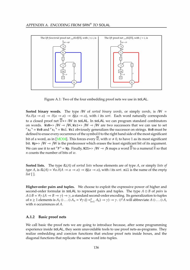
APPENDIX A. ENCODING FROM SRN= TO SOLAL
The lift-functorial proof net j≤iElf[Π], with j ≤ i, is The lift proof net j<iEl[Π], with j < i, is
⊸R
i§R
I
⊸L I
Cut
Π
j§L
j§A⊸i§B
i§B
B
A⊸BA
⊸R
i!R
I
⊸L I
Cut
Π
j§L
j§A⊸i!B
i§B
B
A⊸BA
Figure A.1: Two of the four embedding proof nets we use in soLAL.
Sorted binary words. The type iW of sorted binary words, or simply words, is iW =
∀α.i!(α⊸ α) ⊸ i!(α⊸ α) ⊸ i§(α⊸ α), with i its sort. Each word naturally corresponds
to a closed proof net w ⊲ ⊢ iW in soLAL. In soLAL we can program standard combinatorson words. Ws0 ⊲ ⊢ jW⊸ jW, Ws1 ⊲ ⊢ jW⊸ jW are two successors that we can use to setps0q = Ws0 and ps1q = Ws1. Ws1 obviously generalizes the successor on strings. Ws0must bedefined to erase every occurrence of the symbol 0 to the right hand side of themost significant
bit of a word, as in [MO04]. This forces every w, with w , 0, to have 1 as its most significantbit. Wp ⊲ ⊢ jW⊸ jW is the predecessor which erases the least significant bit of its argument.
We can use it to set pPq = Wp. Finally, W2S ⊲ ⊢ jW⊸ jSmaps a word w to a numeral n so thatn counts the number of bits of w.
Sorted lists. The type iL(A) of sorted lists whose elements are of type A, or simply lists oftype A, is iL(A) = ∀α.i!(A⊸ α⊸ α)⊸ i§(α⊸ α), with i its sort. nil is the name of the emptylist [ ].
Higher-order pairs and tuples. We choose to exploit the expressive power of higher andsecond-order formulæ in soLAL to represent pairs and tuples. The type A ⊙ B of pairs isA⊙B = ∀γ.(A⊸ B⊸ γ)⊸ γ, a standard second-order encoding. Its generalization to tuplesof n ≥ 1 elements is A1 ⊙ . . .⊙An = ∀γ.((⊸n
k=1Ak)⊸ γ)⊸ γ. ⊙
nAwill abbreviate A⊙ . . .⊙A,with n occurrences of A.
A.1.2 Basic proof nets
We call basic the proof nets we are going to introduce because, after some programmingexperience inside soLAL, they seem unavoidable tools to use proof nets-as-programs. Theyrealize embedding and coercion functions that enclose proof nets inside boxes, and thediagonal functions that replicate the same word into tuples.
136
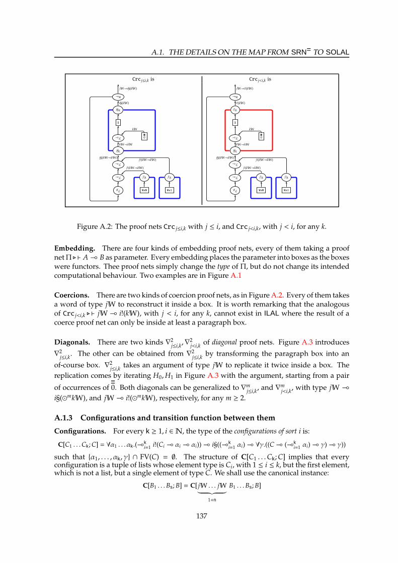
A.1. THE DETAILS ON THE MAP FROM SRN= TO SOLAL
Crcj≤i,k is Crcj<i,k is
⊸R
i§R
I
⊸L 0
j§L
⊸L
⊸L j!R j!R
∀L Ws0 Ws1
jW⊸i§(kW)
i§(kW)
kW⊸kW
j§(kW⊸kW)
kW
j!(kW⊸kW)
j!(kW⊸kW)
⊸R
i!R
I
⊸L 0
j§L
⊸L
⊸L j!R j!R
∀L Ws0 Ws1
jW⊸i!(kW)
i!(kW)
kW⊸kW
j§(kW⊸kW)
kW
j!(kW⊸kW)
j!(kW⊸kW)
Figure A.2: The proof nets Crc j≤i,k with j ≤ i, and Crc j<i,k, with j < i, for any k.
Embedding. There are four kinds of embedding proof nets, every of them taking a proofnetΠ ⊲ ⊢ A⊸ B as parameter. Every embedding places the parameter into boxes as the boxeswere functors. Thee proof nets simply change the type of Π, but do not change its intendedcomputational behaviour. Two examples are in Figure A.1
Coercions. There are two kinds of coercion proof nets, as in Figure A.2. Every of them takesa word of type jW to reconstruct it inside a box. It is worth remarking that the analogousof Crc j<i,k ⊲ ⊢ jW⊸ i!(kW), with j < i, for any k, cannot exist in ILAL where the result of acoerce proof net can only be inside at least a paragraph box.
Diagonals. There are two kinds ∇2j≤i,k,∇2
j<i,kof diagonal proof nets. Figure A.3 introduces
∇2j≤i,k
. The other can be obtained from ∇2j≤i,k
by transforming the paragraph box into an
of-course box. ∇2j≤i,k
takes an argument of type jW to replicate it twice inside a box. The
replication comes by iterating H0,H1 in Figure A.3 with the argument, starting from a pair
of occurrences of 0. Both diagonals can be generalized to ∇mj≤i,k
, and ∇mj<i,k
, with type jW ⊸
i§(⊙mkW), and jW⊸ i!(⊙mkW), respectively, for any m ≥ 2.
A.1.3 Configurations and transition function between them
Configurations. For every k ≥ 1, i ∈N, the type of the configurations of sort i is:
C[C1 . . .Ck;C] = ∀α1 . . . αk.(⊸ki=1 i!(Ci ⊸ αi ⊸ αi))⊸ i§((⊸k
i=1 αi)⊸ ∀γ.((C⊸ (⊸ki=1 αi)⊸ γ)⊸ γ))
such that α1, . . . , αk, γ ∩ FV(C) = ∅. The structure of C[C1 . . .Ck;C] implies that everyconfiguration is a tuple of lists whose element type is Ci, with 1 ≤ i ≤ k, but the first element,which is not a list, but a single element of type C. We shall use the canonical instance:
C[B1 . . .Bs;B] = C[ jW . . . jW︸ ︷︷ ︸
1+n
B1 . . .Bs;B]
137
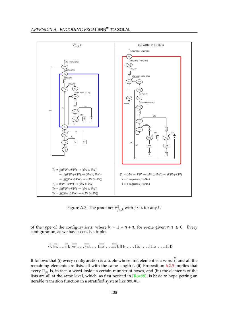
APPENDIX A. ENCODING FROM SRN= TO SOLAL
∇2j≤i,k
is Hi, with i ∈ 0, 1, is
⊸R
i§R
I
⊸L ∀R
⊸R
I
⊸L
⊸L 0 0
j§L
⊸L
⊸L H0 H1
∀L
jW⊸i§(kW⊙kW)
i§(kW⊙kW)
kW⊙kW
T1
T3
T0
(kW⊸kW⊸γ)⊸γ
γ
kW⊙kW
kW
kW
T2
T2
jW
j!R
⊸R
I
⊸L ⊸R
⊸R
∀L ∀R
⊸R
I
⊸L
⊸L I I
⊸L I ⊸L I
Cut Cut
J J
j!((kW⊙kW)⊸(kW⊙kW))
(kW⊙kW)⊸(kW⊙kW)
kW⊙kW
T1
kW⊙kW
(kW⊸kW⊸γ)⊸γ
γ
kW
kW
kW⊸kW⊸(kW⊙kW)
kW
kW
kW kW
T0 = j!((kW ⊙ kW)⊸ (kW ⊙ kW))
⊸ j!((kW ⊙ kW)⊸ (kW ⊙ kW))
⊸ j§((kW ⊙ kW)⊸ (kW ⊙ kW))
T1 = (kW ⊙ kW)⊸ (kW ⊙ kW)
T2 = j!((kW ⊙ kW)⊸ (kW ⊙ kW))
T3 = j§((kW ⊙ kW)⊸ (kW ⊙ kW))
T1 = (kW⊸ kW⊸ (kW ⊙ kW))⊸ (kW ⊙ kW)
i = 0 requires J is Ws0
i = 1 requires J is Ws1
Figure A.3: The proof net ∇2j≤i,k
with j ≤ i, for any k.
of the type of the configurations, where k = 1 + n + s, for some given n, s ≥ 0. Everyconfiguration, as we have seen, is a tuple:
〈r, [a1, . . . , ar], [n11, . . . , n1r], . . . , [nn1, . . . , nnr], [Π11, . . . ,Π1r], . . . , [Πs1, . . . ,Πsr]〉
It follows that (i) every configuration is a tuple whose first element is a word r, and all theremaining elements are lists, all with the same length r, (ii) Proposition 6.2.5 implies thatevery Πpq is, in fact, a word inside a certain number of boxes, and (iii) the elements of thelists are all at the same level, which, as first noticed in [Rov99], is basic to hope getting aniterable transition function in a stratified system like soLAL.
138

A.1. THE DETAILS ON THE MAP FROM SRN= TO SOLAL
Pre-Configurations. For every k ≥ 1, the type of the pre-configurations is:
PC[α1 . . . αk;C1 . . .Ck;C] = ∀γ.((C⊸ (⊸ki=1 T[αi;Ci])⊸ γ)⊸ γ)
T[α;C] = ∀β.((U[α;C]⊸ β)⊸ β)
U[α;C] = (C⊸ α⊸ α)⊸ (C⊸ C)⊸ C⊸ α (tuple of couples of (C⊸ C) and C)
such that α1, . . . , αk, γ∩FV(C) = ∅. We shall use the following canonical instance of the typeof the pre-configurations:
PC[α0 . . . αn+s;B1 . . .Bs;B] = PC[α0 . . . αn+s; iW . . . iW︸ ︷︷ ︸1+n
B1 . . .Bs;B]
where k = 1 + n + s, for some n, s ≥ 0,m ≥ 1. Every pre-configuration is in fact a tuple oftuples:
〈r, 〈a1, [a2, . . . , ar]〉 , 〈n11, [n12, . . . , n1r]〉, . . . , 〈nn1, [nn2, . . . , nnr]〉 , 〈Π11, [Π12, . . . ,Π1r]〉, . . . , 〈Πs1, [Πs2, . . . ,Πsr]〉〉
The proof net C2C1+n;s[F, F′]. The root of its definition is in Figure A.4. Its main componentsare the proof nets C2PC1+n;s and PC2C1+n;s, which split the move “configuration to configura-tion” in two simpler steps: “configuration to pre-configuration” and “pre-configuration toconfiguration”.C2C1+n;s requires two parameters F and F′. Fmust be a closed proof net of typeC⊸ C, for
some C. It will be either a successor on words, mapped on the first list of the configurationin input to get the next value of the step function, or a function identity, mapped along allthe remaining lists of the configuration in input. F′ is a closed proof net that is used as a stepfunction by PC2C1+n;s. Looking back to Proposition 6.2.5, instances of F′ must be ph0q andph1q, relative the recursive function f 1+n;s of SRN we want to represent. Both ph0q and ph1qhave type (⊸n
k=0jW)⊸ (⊸s
k=1Bk)⊸ B⊸ B, with B1 . . .Bs,B instantiated by jW.
The proof net C2PC1+n;s[F]. It is defined by the set of proof nets in Figure A.5, A.6, A.7, andA.8. The proof net takes a configuration in input, separates the first component of every listin the configuration from its tail, and maps F along the tail. In particular, if F is a successoron words, all the words in the tail get increased.
Specifically, Figure A.8 contains a step function StC2PC[F] that takes a list and appliesF : C⊸ C (F is the successor or the identity) to each element of the list but the head.
The proof net PC2C1+n;s[F′]. It is defined by the set of proof nets in Figure A.9, A.10, A.11,
A.12. F′ has type (⊸nk=0
jW) ⊸ (⊸sk=1
Bk) ⊸ B ⊸ B. The graph with name “1 + n + s Wnodes” in Figure A.11 contains only as many as 1 + n + s nodesW.
A.1.4 The iteration
Finally, we can define It1+n,s[H0,H1,G] that iterates C2C1+n;s[F, F′] from an initial configura-tion, for a sufficient number of times. From the last configuration the iteration produces wecan extract the word that represents the result of p f 1+n;sq. We have already described (at thebeginning of this Appendix) the interaction among the proof nets It1+n,s[H0,H1,G], W2C1+n;s,C2C1+n;s, C2FC1+n;s, and FC2W1+n;s. The last two proof nets use final configurations, that we havenot defined yet. We proceed by first setting the final configurations, and, then, by bottom upintroducing It1+n,s[H0,H1,G].
139

APPENDIX A. ENCODING FROM SRN= TO SOLAL
C2C1+n;s[F,F′] is
⊸R
∀R
∀R
⊸R
⊸R
i§R
⊸R
⊸R
∀R
I
⊸L I
⊸L
Cut ⊸L I I
PC2C1+n;s[F′]
i§L
C2PC1+n;s[F]
I I I
C[B1...Bs ;B]⊸C[B1 ...Bs ;B]
C[B1 ...Bs ;B]
1+n+s
(⊸n
k=0i!( jW⊸αk⊸αk)
)⊸(⊸s
k=1i!(Bk⊸αk+n⊸αk+n)
)⊸i§((⊸n+s
k=0αk)⊸∀γ.((B⊸(⊸n+s
k=0αk)⊸γ)⊸γ)
)
1+n+s
i§((⊸n+sk=0αk)⊸∀γ.((B⊸(⊸n+s
k=0αk)⊸γ)⊸γ))
1+n+s
∀γ.((B⊸(⊸n+sk=0αk)⊸γ)⊸γ)
(B⊸(⊸n+sk=0αk)⊸γ)⊸γ
1+n+s
1+n+s
i§((⊸n+sk=0αk)⊸PC[α0...αn+s ;B1 ...Bs ;B])
PC[α0...αn+s;B1 ...Bs ;B]
PC2C1+n;s[F′] is in Figure A.9.
C2PC1+n;s[F] is in Figure A.5.
Figure A.4: The proof net C2C1+n;s[F, F′]
Final configurations. For every k ≥ 1, the type of the final configurations is:
FC[C1 . . .Ck;C] = ∀α1 . . . αkγ.(⊸ki=1 i!(Ci ⊸ αi ⊸ αi))⊸ i§((⊸k
i=1 αi)⊸ (C⊸ (⊸ki=1 αi)⊸ γ)⊸ γ)
such that α1, . . . , αk, γ ∩ FV(C) =. The difference with the type of the configurations is theextrusion of the universal quantifier on γ. We shall use the following canonical instance of thetype of the final configurations, for some given n, s ≥ 0, and m ≥ 1:
FC[B1 . . .Bs;B] = FC[iW . . . iW︸ ︷︷ ︸1+n
B1 . . .Bs;B]
140

A.1. THE DETAILS ON THE MAP FROM SRN= TO SOLAL
C2PC1+n;s[F] is
J in Figure A.6
H in Figure A.7
i§((⊸n+s
k=0αk)⊸PC[α0...αn+s ;B1 ...Bs ;B]
)
i§((⊸n
k=0T[αk ; jW]
)⊸(⊸s
k=1T[αk+n ;Bk ]
)⊸PC[α0...αn+s;B1 ...Bs ;B]
)
C[B1 ...Bs ;B]
i!( jW⊸α1⊸α1)...i!( jW⊸αnk⊸αn)
i!(B1⊸αn+1⊸αn+1)...(Bs⊸αn+s⊸αn+s)
Figure A.5: The proof net C2PC1+n;s[F]
The final configurations are a necessary step to extract, with the correct typing, the firstcomponent of a configuration, that will represent the result of an iteration.
The proof net It1+n,s[H0,H1,G]. Assuming H0,H1,G be proof nets such that:
Hi ⊲ ⊢ jW⊸ (⊸nk=1 jW)⊸ (⊸s
k=1 Bk)⊸ B⊸ B (i ∈ 0, 1)
G ⊲ ⊢ (⊸nk=1 jW)⊸ (⊸s
k=1 Bk)⊸ B
It1+n,s[H0,H1,G] is in FigureA.13, A.14, A.15, andA.16. We have alreadydescribed the computationalbehaviour of this proof net.
The proof net W2C1+n;s. It is in Figure A.17 and A.18.We conclude with some comments on the structure of the proof nets in Figure A.18. For every 1 ≤
q ≤ n, Ss(W2S kq) is obtained by applying Ss ⊲ iS⊸ iS to the result of the application of W2S ⊲ jW⊸ iSto an argument of type jW, represented by kq in the name of the proof net. An analogous definitionholds for every Ss(W2S hp), with 1 ≤ p ≤ s.
The proof net L2C1+n;s[F]. Assuming that F be a proof net such that F ⊲ ⊢ B, L2C1+n;s[F] is inFigure A.19, A.20, and A.21. It takes 1 + n + s lists, each with as many elements as the number ofdigits of the main argument of f 1+n;s, augmented by 1, and yields the expected configurations.
141

APPENDIX A. ENCODING FROM SRN= TO SOLAL
i§R
⊸R
⊸R
⊸R
⊸R
⊸R
I
⊸L
⊸L
⊸L
⊸L
⊸L I I I I I
⊸L I ⊸L I ⊸L I ⊸L I ⊸L I
Cut Cut Cut Cut Cut
BaC2PC[0] BaC2PC[0] BaC2PC[0] BaC2PC[0] BaC2PC[0]
i§L
i§((⊸n+sk=0αk)⊸PC[α0...αn+s ;B1 ...Bs ;B])
n
s
PC[α0...αn+s;B1 ...Bs ;B]=∀γ.(B⊸(⊸nk=0
T[αk; jW])⊸(⊸sk=1
T[αk+n ;Bk])⊸γ)⊸γ
s
n
V1 as in Figure A.7
U1s
U11
T1n
T11
T10
α0 α1 αn αn+1 αn+s
BaC2PC[G] is in Figure A.8.
T1k = T[αk; jW] (0 ≤ k ≤ n)
U1k = T[αk+n ;Bk] (1 ≤ k ≤ s)
Figure A.6: The proof net J for C2PC1+n;s[F]
142
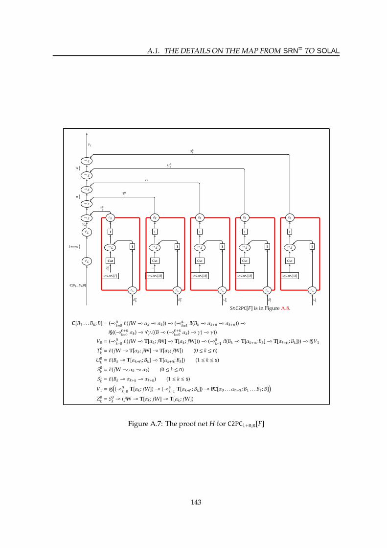
A.1. THE DETAILS ON THE MAP FROM SRN= TO SOLAL
⊸L
⊸L
⊸L
⊸L
⊸L i!R i!R i!R i!R i!R
∀L I I I I I
⊸L I ⊸L I ⊸L I ⊸L I ⊸L I
∀L Cut Cut Cut Cut Cut
StC2PC[F] StC2PC[Id] StC2PC[Id] StC2PC[Id] StC2PC[Id]
i!L i!L i!L i!L i!L
V1
s
n
V0
1+n+s
C[B1 ...Bs ;B]
Z00
S00
...
S01 S0n S1
1 S1s
U0s
U01
T0n
T01
T00
StC2PC[F] is in Figure A.8.
C[B1 . . .Bs;B] = (⊸nk=0 i!( jW⊸ αk ⊸ αk))⊸ (⊸s
k=1i!(Bk ⊸ αk+n ⊸ αk+n))⊸
i§((⊸n+sk=0 αk)⊸ ∀γ.((B⊸ (⊸n+s
k=0 αk)⊸ γ)⊸ γ))
V0 = (⊸nk=0 i!( jW⊸ T[αk; jW]⊸ T[αk; jW]))⊸ (⊸s
k=1 i!(Bk ⊸ T[αk+n ;Bk]⊸ T[αk+n ;Bk]))⊸ i§V1
T0k= i!( jW⊸ T[αk; jW]⊸ T[αk; jW]) (0 ≤ k ≤ n)
U0k= i!(Bk ⊸ T[αk+n ;Bk]⊸ T[αk+n;Bk]) (1 ≤ k ≤ s)
S0k = i!( jW⊸ αk ⊸ αk) (0 ≤ k ≤ n)
S1k = i!(Bk ⊸ αk+s ⊸ αk+s) (1 ≤ k ≤ s)
V1 = i§((⊸n
k=0 T[αk; jW])⊸ (⊸sk=1 T[αk+n ;Bk])⊸ PC[α0 . . . αn+s;B1 . . .Bs;B]
)
Z0k= S0
k⊸ ( jW⊸ T[αk; jW]⊸ T[αk; jW])
Figure A.7: The proof net H for C2PC1+n;s[F]
143

APPENDIX A. ENCODING FROM SRN= TO SOLAL
BaC2PC[G] is StC2PC[F] is
⊸R
∀R
⊸R
I
⊸L I
⊸L
⊸L
⊸L ⊸R Id G
W ⊸R
I
α⊸T[α;C]
T[α;C]
(U[α;C]⊸β)⊸β
β
α⊸β
α
C
C⊸C
C⊸α⊸α
U[α;C]⊸β
⊸R ⊸R
⊸R ⊸R
⊸R ⊸R
∀R ⊸R
⊸R I
I ⊸L I
⊸L I ⊸L I
⊸L ⊸L ⊸L I
⊸L
⊸L I F I ∀L
(C⊸α⊸α)⊸C⊸T[α;C]⊸T[α;C]
C⊸T[α;C]⊸T[α;C]
T[α;C]⊸T[α;C]
T[α;C]
(U[α;C]⊸β)⊸β
β
((C⊸α⊸α)⊸(C⊸C)⊸C⊸α⊸α)⊸α
(C⊸C)⊸C⊸α⊸α
C⊸α⊸α
α
α
C
C⊸C
C⊸α⊸α
(C⊸α⊸α)⊸(C⊸C)⊸C⊸α⊸α
α
C
C
T[α;C] = ∀β.((U[α;C]⊸ β)⊸ β)
U[α;C] = (C⊸ α⊸ α)⊸ (C⊸ C)⊸ C⊸ α
Figure A.8: The proof nets BaC2PC[G] and StC2PC[F]
PC2C1+n;s[F′] is:
⊸R
I
⊸L
∀L H in Figure A.10
PC[α0...αn+s;B1 ...Bs ;B]⊸((B⊸(⊸n+sk=0αk)⊸γ)⊸γ
(B⊸(⊸n+sk=0αk)⊸γ)⊸γ
TB⊸(⊸n
k=0T[αk; jW])⊸(⊸s
k=1T[αk+n ;Bk])⊸((B⊸(⊸n+s
k=0αk)⊸γ)⊸γ)
PC[α0...αn+s;B1 ...Bs ;B]=∀γ.(B⊸(⊸nk=0
T[αk; jW])⊸(⊸sk=1
T[αk+n ;Bk ])⊸γ)⊸γ
T = (B⊸ (⊸nk=0 T[αk; jW])⊸ (⊸s
k=1T[αk+n ;Bk])⊸ ((B⊸ (⊸n+s
k=0αk)⊸ γ)⊸ γ))⊸ ((B⊸ (⊸n+s
k=0αk)⊸ γ)⊸ γ)
Figure A.9: The proof net PC2C1+n;s[F′]
144

A.1. THE DETAILS ON THE MAP FROM SRN= TO SOLAL
H for PC2C1+n;s[F′] is:
⊸R
⊸R
⊸R
⊸R
⊸R
⊸R
I
⊸L I I I I
⊸L ⊸L ⊸L ⊸L
∀L ∀L ∀L ∀L ∀L J in Figure A.11
B⊸(⊸nk=0
T[αk; jW])⊸(⊸sk=1
T[αk+n ;Bk ])⊸((B⊸(⊸n+sk=0αk)⊸γ)⊸γ)
s
n
(B⊸(⊸n+sk=0αk)⊸γ)⊸γ
T′s
T′1 Tn T1 T0
V′1 V1
U[α0; jW]⊸V1
Tk = (U[αk; jW]⊸ Vk+1)⊸ Vk+1 (0 ≤ k ≤ n)
T′k = (U[αn+k;Bk]⊸ V′k+1)⊸ V′k+1 (1 ≤ k ≤ s)
Vk = U[αk; jW]⊸ (⊸nm=k+1 U[αm; jW])⊸ (⊸s
m=1 U[αn+m;Bm])⊸ ((B⊸ (⊸n+sm=0 αm)⊸ γ)⊸ γ) (0 ≤ k ≤ n)
V′k = U[αn+k;Bk]⊸ (⊸sm=k+1 U[αn+m;Bm])⊸ ((B⊸ (⊸n+s
m=0 αm)⊸ γ)⊸ γ) (1 ≤ m ≤ s)
Figure A.10: The proof net H for PC2C1+n;s[F′]
145

APPENDIX A. ENCODING FROM SRN= TO SOLAL
J for PC2C1+n;s[F′] is:
⊸R
⊸R
⊸R
⊸R
⊸R
⊸R
⊸R
⊸R
⊸R
⊸R
⊸R
⊸R
⊸R
⊸R
⊸R
⊸R
⊸R
⊸R
⊸R
⊸R
Cut
1+n+s W nodes K in Figure A.12
(⊸nk=0
U[αk; jW])⊸(⊸sk=1
U[αk+n ;Bk ])⊸((B⊸(⊸n+sk=0αk)⊸γ)⊸γ)
n
(⊸sk=1
U[αk+n;Bk ])⊸((B⊸(⊸n+sk=0αk)⊸γ)⊸γ)
s
U[αn+s;Bs ]⊸((B⊸(⊸n+sk=0αk)⊸γ)⊸γ)
(B⊸(⊸n+sk=0αk)⊸γ)⊸γ
B
Figure A.11: The proof net J for PC2C1+n;s[F′]
146

A.1. THE DETAILS ON THE MAP FROM SRN= TO SOLAL
K for PC2C1+n;s[F′] is:
⊸R I
I ⊸L
⊸L ⊸L
⊸L ⊸L
⊸L ⊸L
⊸L ⊸L
⊸L I I I I I ⊸L I I I I I I
⊸L Cut
F′
(B⊸(⊸n+sk=0αk)⊸γ)⊸γ
γ
s
n
s
n
αn+s
αn+1
αn
α1
α0
B
B
Bs
B1
jW
jW
jW
Figure A.12: The proof net K for PC2C1+n;s[F′]
It1+n,s[H0,H1,G] is
⊸R
⊸R
⊸R
K in Figure A.14
I I I
⊸L I ⊸L I ⊸L I
Crc j≤i, j Crc j≤i, j Crc j≤i, j
jW⊸(⊸nk=1
jW)⊸(⊸sk=1
i§3 j§Bk)⊸i§4B (i> j)
n
(⊸sk=1
i§3 j§Bk)⊸i§4B
i§( jW)i§( jW)
i§( jW)
Figure A.13: The proof net It1+n,s[H0,H1,G].
147

APPENDIX A. ENCODING FROM SRN= TO SOLAL
i§R
i§R
J in Figure A.15
i§L i§L i§L i§L i§L
i§L i§L i§L i§L i§L
. . .
i§4B (i> j)
i§3B
i§2B
jW⊙ jW
...i§ j§( jW)... i§ j§B1
i§ j§Bs
i§( jW⊙ jW) ...i§2 j§( jW)... i§2 j§B1 i§2 j§Bs
︸︷︷︸s
︸︷︷︸n
⊸L I ⊸L I ⊸L I
i≤iElf[∇2j≤i, j
] ElfCoerce ElfCoerce
T2 T3 T3
i§2( jW⊙ jW)
i§3 j§( jW) i§3 j§( jW)
i§( jW) i§( jW) i§( jW)
T2 = i§( jW)⊸ i§2( jW ⊙ jW)
T3 = i§( jW)⊸ i§3 j§( jW)
Figure A.14: The proof net K for It1+n,s[H0,H1,G].
148
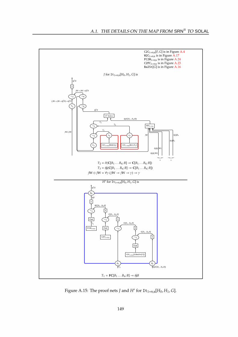
A.1. THE DETAILS ON THE MAP FROM SRN= TO SOLAL
C2C1+n;s[F,G] is in Figure A.4W2C1+n;s is in Figure A.17FC2W1+n;s is in Figure A.24C2FC1+n;s is in Figure A.23Ba2St[G] is in Figure A.16
J for It1+n,s[H0,H1,G] is
I
⊸L ⊸R
∀L ⊸R
H′ below
⊸L W2C1+n;s
⊸L i!R i!R
∀L C2C1+n;s[Ws0,H0] C2C1+n;s[Ws1,H1]
i§2B
( jW⊸ jW⊸i§2B)⊸i§2B
jW⊙ jW
i§2B
︸︷︷︸n
︸︷︷︸s
i§ j§( jW)
i§ j§( jW)
i§ j§B1
i§ j§Bs
jW⊸ jW⊸i§2B
i§(C[B1...Bs ;B])
T3
T2
T2
jW
T2 = i!(C[B1 . . .Bs;B]⊸ C[B1 . . .Bs;B])
T3 = i§(C[B1 . . .Bs;B]⊸ C[B1 . . .Bs;B])
jW ⊙ jW = ∀γ.( jW⊸ jW⊸ γ)⊸ γ
H′ for It1+n,s[H0,H1,G] is
i§R
I
⊸L I
Cut ⊸L I
FC2W1+n;s Cut ⊸L I
C2FC1+n;s ⊸L I
Cut
C2C1+n;s[Id;Ba2St[G]]
i§L i§L
i§2B
i§B
T1
FC[B1 ...Bs ;B]
C[B1 ...Bs ;B]
C[B1 ...Bs ;B]
C[B1 ...Bs ;B]
T3 i§(C[B1...Bs ;B])
T1 = FC[B1 . . .Bs;B]⊸ i§B
Figure A.15: The proof nets J and H′ for It1+n,s[H0,H1,G].
149

APPENDIX A. ENCODING FROM SRN= TO SOLAL
Ba2St for It1+n,s[H0,H1,G]is
⊸R
⊸R
⊸R
⊸R
⊸R
⊸R
⊸L
⊸L
⊸L
⊸L I I I I
W W G
n
s
s
n
Figure A.16: The proof net Ba2St for It1+n,s[H0,H1,G]
150
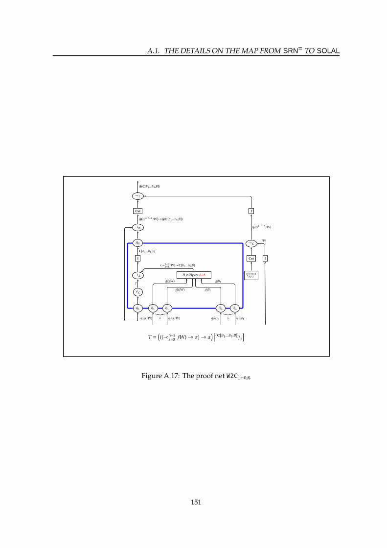
A.1. THE DETAILS ON THE MAP FROM SRN= TO SOLAL
⊸L
Cut I
⊸R
i§R ⊸L
I Cut I
⊸L H in Figure A.18 ∇1+n+sj≤i, j
∀L
i§L i§L i§L i§L i§L
i§(C[B1 ...Bs ;B])
i§(⊙1+n+s jW)⊸i§(C[B1 ...Bs ;B])
C[B1 ...Bs ;B]
(⊸n+sk=0
jW)⊸C[B1...Bs ;B]
Tj§( jW)
j§( jW) j§B1
j§Bs
i§ j§( jW) i§ j§( jW) i§ j§B1 i§ j§Bs
jW
i§(⊙1+n+s jW)
︸︷︷︸s
︸︷︷︸n
T =(((⊸n+s
k=0jW)⊸ α)⊸ α
) [(C[B1...Bs ;B])/α
]
Figure A.17: The proof net W2C1+n;s
151

APPENDIX A. ENCODING FROM SRN= TO SOLAL
⊸R
⊸R
⊸R
⊸R
⊸R
L2C1+n;s[0]
n︷︸︸︷. . .
s︷︸︸︷. . .
⊸L ⊸L ⊸L ⊸L ⊸L
⊸L j§R ⊸L ⊸L ⊸L ⊸L
S2L 0 Ss(W2S k0) S2L I Ss(W2S k1) S2L I Ss(W2S kn) S2L I Ss(W2S h1) S2L I Ss(W2S hs)
(⊸n+sk=0
jW)⊸C[B1...Bs ;B]
n
(⊸sk=1
jW)⊸C[B1...Bs ;B]
s
jW
iL(Bs)
iL(B1)iL( jW)
iL( jW)
iL( jW)
C[B1 ...Bs ;B]
T2 T2 T2 T31 T3s
iS
j§( jW) j§( jW) j§B1 j§Bs
T2 = j§( jW)⊸ iS⊸ iL( jW) T3k = j§(Bk)⊸ iS⊸ iL(Bk) (1 ≤ k ≤ s)
Figure A.18: The proof net H for W2C1+n;s
152
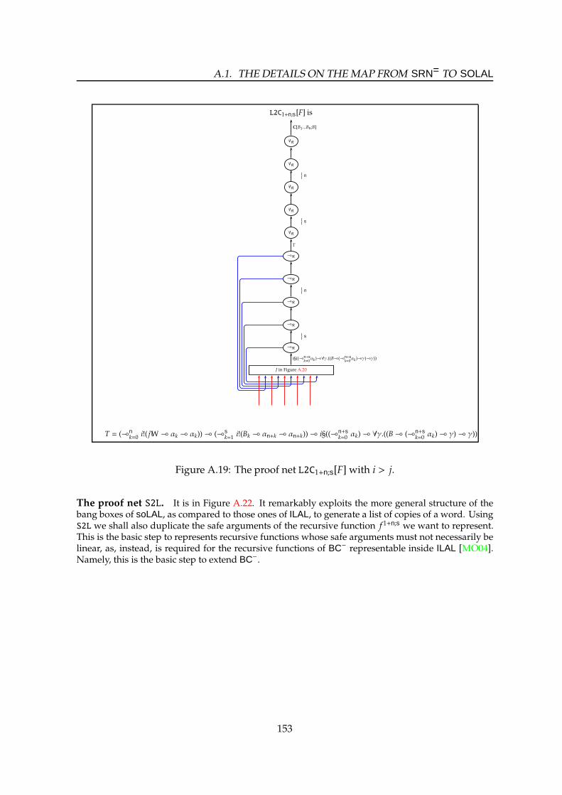
A.1. THE DETAILS ON THE MAP FROM SRN= TO SOLAL
L2C1+n;s[F] is
∀R
∀R
∀R
∀R
∀R
⊸R
⊸R
⊸R
⊸R
⊸R
J in Figure A.20
C[B1...Bs ;B]
n
s
T
n
s
i§((⊸n+sk=0αk)⊸∀γ.((B⊸(⊸n+s
k=0αk)⊸γ)⊸γ))
T = (⊸nk=0 i!( jW⊸ αk ⊸ αk))⊸ (⊸s
k=1 i!(Bk ⊸ αn+k ⊸ αn+k))⊸ i§((⊸n+sk=0 αk)⊸ ∀γ.((B⊸ (⊸n+s
k=0 αk)⊸ γ)⊸ γ))
Figure A.19: The proof net L2C1+n;s[F] with i > j.
The proof net S2L. It is in Figure A.22. It remarkably exploits the more general structure of thebang boxes of soLAL, as compared to those ones of ILAL, to generate a list of copies of a word. UsingS2L we shall also duplicate the safe arguments of the recursive function f 1+n;s we want to represent.This is the basic step to represents recursive functions whose safe arguments must not necessarily belinear, as, instead, is required for the recursive functions of BC− representable inside ILAL [MO04].Namely, this is the basic step to extend BC−.
153

APPENDIX A. ENCODING FROM SRN= TO SOLAL
i§R
H in Figure A.21
n︷︸︸︷. . .
s︷︸︸︷. . .
i§L i§L i§L i§L i§L
⊸L ⊸L ⊸L ⊸L ⊸L
∀L I ∀L I ∀L I ∀L I ∀L I
T0 T′0
T1 T′1
Tn T′n Un+1 U′n+1 Un+s U′n+s
i§((⊸n+sk=0αk)⊸∀γ.((B⊸(⊸n+s
k=0αk)⊸γ)⊸γ))
((⊸n+sk=0αk)⊸∀γ.((B⊸(⊸n+s
k=0αk)⊸γ)⊸γ))
α0⊸α0
α1⊸α1
αn⊸αn
αn+1⊸αn+1
αn+s⊸αn+s
T′′0
T′′1 T′′n U′′n+1 U′′n+s
Tk =∀αk.i!( jW⊸ αk ⊸ αk)⊸ i§(αk ⊸ αk) (0 ≤ k ≤ n)
T′k =i!( jW⊸ αk ⊸ αk) (0 ≤ j ≤ n)
T′′k =i!( jW⊸ αk ⊸ αk)⊸ i§(αk ⊸ αk) (0 ≤ k ≤ n)
Uk =∀αk.i!(Bk ⊸ αk ⊸ αk)⊸ i§(αk ⊸ αk) (1 ≤ k ≤ s)
U′k =i!(Bk ⊸ αk ⊸ αk) (1 ≤ k ≤ s)
U′′k =i!(Bk ⊸ αk ⊸ αk)⊸ i§(αk ⊸ αk) (1 ≤ k ≤ s)
Figure A.20: The proof net J for L2C1+n;s[F].
154

A.1. THE DETAILS ON THE MAP FROM SRN= TO SOLAL
⊸R
⊸R
⊸R
⊸R
⊸R
∀R
⊸R
I
⊸L
⊸L
⊸L
⊸L
⊸L
⊸L I I
n︷︸︸︷. . . I I
s︷︸︸︷. . . I
F ⊸L ⊸L ⊸L ⊸L ⊸L
I I I I I
(⊸n+sk=0αk)⊸∀γ.((B⊸(⊸n+s
k=0αk)⊸γ)⊸γ)
(⊸n+sk=1αk)⊸∀γ.((B⊸(⊸n+s
k=0αk)⊸γ)⊸γ)
n
(⊸n+sk=n+1
αk)⊸∀γ.((B⊸(⊸n+sk=0αk)⊸γ)⊸γ)
s
∀γ.((B⊸(⊸n+sk=0αk)⊸γ)⊸γ)
(B⊸(⊸n+sk=0αk)⊸γ)⊸γ
γ
α0
α1
αn
αn+1
αn+s
B
α0 α1 αn αn+1 αn+s
α0⊸α0 αn⊸αs
Figure A.21: The proof net H for L2C1+n;s[F].
155
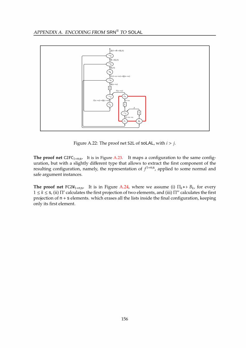
APPENDIX A. ENCODING FROM SRN= TO SOLAL
⊸R
⊸R
∀R
⊸R
I
⊸L i!R
∀L I
⊸L I
i!L j§L
j§A⊸iS⊸iL(A)
iS⊸iL(A)
iL(A)
i!(A⊸α⊸α)⊸i§(α⊸α)
i§(α⊸α)
i!(α⊸α)⊸i§(α⊸α) α⊸α
A⊸α⊸α
i!(α⊸α)
A
Figure A.22: The proof net S2L of soLAL, with i > j.
The proof net C2FC1+n;s. It is in Figure A.23. It maps a configuration to the same config-uration, but with a slightly different type that allows to extract the first component of theresulting configuration, namely, the representation of f 1+n;s, applied to some normal andsafe argument instances.
The proof net FC2W1+n;s. It is in Figure A.24, where we assume (i) Πk ⊲ ⊢ Bk, for every1 ≤ k ≤ s, (ii)Π′ calculates the first projection of two elements, and (iii)Π′′ calculates the firstprojection of n + s elements. which erases all the lists inside the final configuration, keepingonly its first element.
156

A.1. THE DETAILS ON THE MAP FROM SRN= TO SOLAL
C2FC1+n;s is
⊸R
∀R
∀R
∀R
⊸R
⊸R
⊸R
⊸R
⊸R
i§R
⊸R ⊸L
⊸R ⊸L
⊸R ⊸L
⊸R ⊸L
⊸R ⊸L
I I I I I I
⊸L ∀L
⊸L ∀L
⊸L ∀L
⊸L ∀L
⊸L I I I I I ∀L
i§L
C[B1 ...Bs ;B]⊸FC[B1 ...Bs ;B]
FC[B1 ...Bs ;B]
1+n+s
∀γ.(⊸nk=0
i!( jW⊸αk⊸αk))⊸(⊸sk=1
i!(Bk⊸αk⊸αk))⊸i§((⊸n+sk=0αk)⊸(B⊸(⊸n+s
k=0αk)⊸γ)⊸γ)
∀γ.(⊸nk=0
i!( jW⊸αk⊸αk))⊸(⊸sk=1
i!(Bk⊸αk⊸αk))⊸i§((⊸n+sk=0αk)⊸(B⊸(⊸n+s
k=0αk)⊸γ)⊸γ)
n
s
i§((⊸n+sk=0αk)⊸(B⊸(⊸n+s
k=0αk)⊸γ)⊸γ)
T
s
n
n
s
(B⊸(⊸n+sk=0αk)⊸γ)⊸γ
s
s
n
n
αn+s
αn+1
αn
α1
α0
i!(Bs⊸αn+s⊸αn+s)
i!(B1⊸α1+n⊸α1+n)
i!( jW⊸αn⊸αn)
i!( jW⊸α1⊸α1)
i!( jW⊸α0⊸α0)
T =i§((⊸n+sk=0 αk)⊸ ∀γ.(B⊸ (⊸n+s
k=0 αk)⊸ γ)⊸ γ)
Figure A.23: The proof net C2FC1+n;s.
157

APPENDIX A. ENCODING FROM SRN= TO SOLAL
j§R
⊸L
⊸L
⊸L
⊸L
⊸L
⊸L 0 0 0 Π1 Πs Π′′
j§L
j§B
B
s
n
(⊸nk=0
jW)⊸(⊸sk=1
Bk)⊸(B⊸(⊸nk=0
jW)⊸(⊸sk=1
Bk)⊸B)⊸B
B⊸(⊸nk=0
jW)⊸(⊸sk=1
Bk)⊸B
Bs
B1
jW
jW
jW
⊸L
⊸L
⊸L
⊸L
⊸L
∀L i!R i!R i!R i!R i!R
∀L Π′ Π′ Π′ Π′ Π′
∀L
∀L
∀L
T1
s
n
T2
s
n
FC[B1 ...Bs ;B]
i!(Bs⊸Bs⊸Bs)
i!(B1⊸B1⊸B1)
i!( jW⊸ jW⊸ jW)
i!( jW⊸ jW⊸ jW)
i!( jW⊸ jW⊸ jW)
T1 = §((⊸nk=0 jW)⊸ (⊸s
k=1Bk)⊸ (B⊸ (⊸n
k=0 jW)⊸ (⊸sk=1
Bk)⊸ B)⊸ B)
T2 = (⊸nk=0 i!( jW⊸ jW⊸ jW))⊸
(⊸sk=1
i!(Bk ⊸ Bk ⊸ Bk))⊸
§((⊸ni=0 jW)⊸ (⊸s
k=1 Bk)⊸ (B⊸ (⊸nk=0 jW)⊸ (⊸s
k=1 Bk)⊸ B)⊸ B)
Figure A.24: The proof net FC2W1+n;s.
158

Index
Abstract rewriting system . . 40Admissible Rules . . . . . . . . . . . 67Affine Logic . . . . . . . . . . . . . . . . 15
Booleans . . . . . . . . . . . . . . . . . . 109Boundary . . . . . . . . . . . . . . . . . . 28Boxes . . . . . . . . . . . . . . . . . . . 26, 28Fuzzy b. . . . . . . . . . . . . . . . . . 107
Chain . . . . . . . see Spindles, C. ofCharacteristic polynomial . 109Church words . . . . . . 92, 98, 110Class-i nodes . . . . . . . . . . 61, 132Composition schema . . . . . . . 18Computational complexity . 13Confluence . . . . . . . . . . . . . 40, 84Context . . . . . . . . . . . . . . . . . . . . 52Canonical, Initial, Final . . . 53Context Semantics . . . . . . . . 52
Contraction . . . . . . . . . . . . . . . . 15Cost of reduction . . . . . . . . . . . 50Critical argument . . . . . . . . . . 19CS-path . . . . . . . . . . . . . . . . . . . . 54Maximal CS-p. . . . . . . . . . . . 54
Curry-Howard corresp. . . . . 13Cut-elimination . 13, 40, 83, 87,
107
DegreeComposition d. . . . . . . . . . . 109Recursion d. . . . . . . . . . . . . . 109
Depth . . . . . . . . . . . . . . . . . . . . . . 30Dereliction . . . . . . . . . . . . . . . . . 15Digging . . . . . . . . . . . . . . . . . . . . 15Downward closure . . . . . . . . . 34
Edge . . . . . . . . . . . . . . . . . . . . . . . 26Reverse e. . . . . . . . . . . . . . . . . 29
Elementary Affine Logic . . . 89,123
Eventually constant . . . . . . . 111Exponential Signature . . . . . . 52
Formulæ . . . . . . . . . . . . . . . . . . . 25Linear f., modal f. . . . . . . . . 25Meta-f. . . . . . . . . . . . . . . . . . . . 25
GraphBoxed g. . . . . . . . . . . . . . . . . . . 26Surface . . . . . . . . . . . . . . . . . . . 33
Hilbert systems . . . . . . . . . . . . 12
Implicit computational com-plexity . . . . . . . . . . . . . . . . . . .18
Indexing . . . . . . . . . . . . . . . . . . 127Indexing, and Canonical i. . 106
Kleene functions . . . . . . . . . . . 18
λ-calculus . . . . . . . . . . . . . . . . . . 11Leivant’s system . . . . . . . . . . . 19Length of formulæ . . . . . . . . . 43Level . . . . . . . . . . . . . . . . . 106, 128Lifting . . . . . . . . . . . . . . . . . . . . 113Light Affine Logic . . . . . . . . . . 17Light Affine Logic by Levels . .
105Light logics . . . . . . . . . . . . . . . . 17Linear kernel . . . . . . . . . . . 29, 83Linear Logic . . . . . . . . . . . . . . . 14Logistic calculi . . . . . . . . . . . . . 12
Modalities . . . . . . . . . . . . . . . . . 25Meta-m. . . . . . . . . . . . . . . . . . . 25
Modules . . . . . . . . . . . . . . . . . . . 32
Natural deduction . . . . . . . . . 12Net bounding function . . . . 109Node . . . . . . . . . . . . . . . . . . . . . . . 26Left and Right n. . . . . . . . . . 31Terminal n. . . . . . . . . . . . 28, 41
Normal form . . . . . . . . . . . . . . . 35Normalization . . . . . . . . . . . . . 34ns . . . . . . . . . . . . . . . . . . . . . . . . . . 34
Garbage Collector ns . . . . . 50Linear ns . . . . . . . . . . . . . . . . . 50Modal ns . . . . . . . . . . . . . . . . . 50
Number of modalities . . . . . . 34
Order . . . . . . . . . . . . . . . . . . . . . . 22Linear o. . . . . . . . . . . . . . . 22, 77
Output bounding function 109
PathCS-path . . . . . . . . see CS-pathExponential p. . . . . . . . . . . . 108Graph-theoretical p. . . . . . . 33
Polarity . . . . . . . . . . . . . . . . . . . . 52Preorder . . . . . . . . . 22, 73, 77, 79Promotion . . . . . . . . . . . . . . . . . 15Proof net . . . . . . . . . . . . . . . . 16, 26Meta-p. . . . . . . . . . . . . . . . . . . 26Primitive p. . . . . . . . . . . . . . . 68Untyped p. . . . . . . . . . . . . . . 133
Quadratic Time . . . . . . . . . . . . 90
Ramified partial order . . . . . . 90Ramified recurrence . . . . . . . . 19Rank . . . . . . . . . . . . . . . . . . . . . . 124Recurrence argument . . . . . . . 19Recursion schema . . . . . . . . . . 18Recursive types . . . . . . . 106, 133Reduction Size . . . . . . . . . . . . . 48Reduction Time . . . . . . . . . . . . 48Representation of programs 92,
98RuleBuilding r. . . . . . . . . . . . . . . . . 26Meta-Building r. . . . . . . . . . . 26Rewriting r. (contexts) . . . . 52Rewriting r. (cuts) . . . . . . . . 34Used r. . . . . . . . . . . . . . . . . . . . 34
Safe Recursion on Notation 19,97, 105
Scott words . . . . . . 106, 111, 133
159
Sensible∞ . . . . . . . . . . . . . . . . . . 81Sequent associated . . . . . . . . . 29Sequent calculus . . . . . . . . 12, 29Serialization . . . . . . . . . . . . . . . . 31Simulation of programs . . . 117Size . . . . . . . . . . . . . . . . . . . . . 30, 41Soft Linear Logic . . . . . . . . 17, 44Spindle . . . . . . . . . . . . 59, 66, 131Chain of s. . . . . . . . . . . . . 60, 66Dangerous chain of s . . . . . 60Dangerous chain of s. . . . . . 66
Stack elements . . . . . . . . . . . . . 52Strategy . . . . . . . . . . . . . . . . . . . . 35
Canonical s. . . . . . . . . . . . . . . 50Closed s. . . . . . . . . . . . . . . 35, 98Fast s. . . . . . . . . . . . . . . . . . . . 120
Stratification . . . . . . . . . . . . . . . 39Weak s. . . . . . . . . . . . . . . . . . . 107
Strong determinacy . . . . . . . . 67Subnet . . . . . . . . . . . . . . . . . . . . . 32Environment s. . . . . . . . . . . . 32
Subsystem . . . . . . . . . . . . . . . . . 33Augmented s. . . . . . . . . . . . . 68Maximal s. . . . . . . . . . . . . 74, 77Natural quotient of s. . . . . . 79Polysize s. . . . . . . . . . . . . . . . . 48
Polystep s. . . . . . . . . . . . . . . . 48Polytime s. . . . . . . . . . . . . . . . 48Saturated s. . . . . 68, 71, 83, 85Sensible s. . . . . . . . . . . . . . . . . 34
Support . . . . . . . . . . . . . . . . . . . 111
Termination . . . . . . . . . . . . . . . . 40Turing machines . . . . . . . . . . . 41
VariableNormal, safe v. . . . . . . . . . . . 19
Weakening . . . . . . . . . . . . . . . . . 15Free w. . . . . . . . . . . . . . . . . . . . 14
Table of Symbols
2ω . . . . . . . . . . . . . . . . . . . . . . 22A→ B . . . . . . . . . . . . . . . . . . 22A<ω . . . . . . . . . . . . . . . . . . . . 22BA . . . . . . . . . . . . . . . . . . . . . . 22Π ⊲ Γ ⊢ C . . . . . . . . . . . . . . . 29ω . . . . . . . . . . . . . . . . . . . . . . . 22≺L1. . . . . . . . . . . . . . . . . . . . . 108
L . . . . . . . . . . . . . . . . . . . . . 108−→x
n. . . . . . . . . . . . . . . . . . . . . 18
|Π| . . . . . . . . . . . . . . . . . . . . . . 30|Π|d . . . . . . . . . . . . . . . . . . . . . 30‖Π‖ . . . . . . . . . . . . . . . . . . . . . 48mA : (Σ ∪ χ) :nB . . . . . . . . . 60mA :Σ :nB . . . . . . . . . . . . . . . 59[Π] . . . . . . . . . . . . . . . . . . . . . 48f ′′(A) . . . . . . . . . . . . . . . . . . . 22
αΠ(v) . . . . . . . . . . . . . . . . . . . 28ARS . . . . . . . . . . . . . . . . . . . . 40
BdΠ. . . . . . . . . . . . . . . . . . . . . . 30
BΠ . . . . . . . . . . . . . . . . . . . . . . 28βΠ(e) . . . . . . . . . . . . . . . . . . . 28bd(Π) . . . . . . . . . . . . . . . . . . . 30BC . . . . . . . . . . . . . . . . . . . . . 19BC– . . . . . . . . . . . . . . . . . . . . 21BC–n;s . . . . . . . . . . . . . . . . . . 21bo(x) . . . . . . . . . . . . . . . . . . . 28
boundary(Π) . . . . . . . . . . . 28BX . . . . . . . . . . . . . . . . . . . . . 29
CC . . . . . . . . . . . . . . . . . . . . . 13co-soLAL . . . . . . . . . . . . . . 120
∂(Π) . . . . . . . . . . . . . . . . . . . . 30∂(x) . . . . . . . . . . . . . . . . . . . . 30∂C(t) . . . . . . . . . . . . . . . . . . . 109∂R(t) . . . . . . . . . . . . . . . . . . . 109deg(p) . . . . . . . . . . . . . . . . . 109
EdΠ. . . . . . . . . . . . . . . . . . . . . . 30
EΠ . . . . . . . . . . . . . . . . . . . . . . 28EXPTIME . . . . . . . . . . . . . . 13
FPTIME . . . . . . . . . . . . . . . . 13
I0 . . . . . . . . . . . . . . . . . . . . . . 107ICC . . . . . . . . . . . . . . . . . . . . 18IEAL . . . . . . . . . . . . . . . 89, 123ILAL . . . . . . . . . . . . . . . . . 2, 17
LALL . . . . . . . . . . . . . . . . . . 105l(e) . . . . . . . . . . . . . . . . . . . . 107LL . . . . . . . . . . . . . . . . . . . . . . . 2LLL . . . . . . . . . . . . . . . . . . . . . . 2L . . . . . . . . . . . . . . . . . . . . . . . 13l(Π) . . . . . . . . . . . . . . . . . . . 107
M (A) . . . . . . . . . . . . . . . . . . 22M<ω(A) . . . . . . . . . . . . . . . . 22MS . . . . . . . . . . . . . . . . . . . . . 29
nbt(l) . . . . . . . . . . . . . . . . . . 109
OΠ(b) . . . . . . . . . . . . . . . . . . . 54obt(l) . . . . . . . . . . . . . . . . . . 109
P . . . . . . . . . . . . . . . . . . . . . . . 33P(A) . . . . . . . . . . . . . . . . . . . 22P<ω(A) . . . . . . . . . . . . . . . . . 22PΠ(b) . . . . . . . . . . . . . . . . . . . 28Pm(~n) . . . . . . . . . . . . . . . . . . . 28Pm(∅) . . . . . . . . . . . . . . . . . . . 28Pm(r?, ~n) . . . . . . . . . . . . . . . . 33Pm(r∗, ~n) . . . . . . . . . . . . . . . . 33PMLTS
. . . . . . . . . . . . . . . . . . . . 91PSPACE . . . . . . . . . . . . . . . 13PTIME . . . . . . . . . . . . . . . . . 13
RΠ(b) . . . . . . . . . . . . . . . . . . . 54R . . . . . . . . . . . . . . . . . . . . . 70R . . . . . . . . . . . . . . . . . . . . . 70R↑ . . . . . . . . . . . . . . . . . . . . . . 70R⋄ . . . . . . . . . . . . . . . . . . . . . . 70
R↑ . . . . . . . . . . . . . . . . . . . . . . 73rk(Π) . . . . . . . . . . . . . . . . . . 124
160

TABLE OF SYMBOLS
S(P) . . . . . . . . . . . . . . . . . . . 68soLAL . . . . . . . . . . . . . 97, 135SLL . . . . . . . . . . . . . . . . . 17, 44SRN . . . . . . . . . . . . 19, 97, 105SRN= . . . . . . . . . . . . . . . . . . 98
SRN– . . . . . . . . . . . . . . . . . . 99SRNn;s . . . . . . . . . . . . . . . . . 19
Td(Π) . . . . . . . . . . . . . . . . . . . 55
VdΠ
. . . . . . . . . . . . . . . . . . . . . 30
VΠ . . . . . . . . . . . . . . . . . . . . . 28
Wd(Π) . . . . . . . . . . . . . . . . . . 55
X . . . . . . . . . . . . . . . . . . . . . . . 25
161

Bibliography
[AC98] Roberto M. Amadio and Pierre-Louis Curien. Domains and lambda-calculi. Cam-bridge University Press, New York, NY, USA, 1998.
[ACP93] Martın Abadi, Luca Cardelli, and Gordon D. Plotkin. Types for Scott numerals.Available athttp://lucacardelli.name/Papers/Notes/scott2.pdf, 1993.
[AR02] Andrea Asperti and Luca Roversi. Intuitionistic light affine logic. ACM Trans.Comput. Log., 3(1):137–175, 2002.
[Asp98] Andrea Asperti. Light affine logic. In LICS, pages 300–308, 1998.
[Bar84] Hendrik Pieter Barendregt. The lambda calculus – Its syntax and Semantics. Number103 in Studies in Logic and the Foundations of Mathematics. North Holland,Amsterdam, 1984.
[BC92] Stephen Bellantoni and Stephen A. Cook. A new recursion-theoretic characteri-zation of the polytime functions. Computational Complexity, 2(2):97–110, 1992.
[BDLM06] Patrick Baillot, Ugo Dal Lago, and Jean-Yves Moyen. On quasi-interpretations,blind abstractions and implicit complexity. CoRR, abs/cs/0608030, 2006.
[BM04] Patrick Baillot and Virgil Mogbil. Soft lambda-calculus: A language for polyno-mial time computation. In FoSSaCS, pages 27–41, 2004.
[BM07] David Baelde and Dale Miller. Least and greatest fixed points in linear logic. InLPAR, pages 92–106, 2007.
[BM10] Patrick Baillot and Damiano Mazza. Linear logic by levels and bounded timecomplexity. Theor. Comp. Sci., 411(2):470–503, 2010.
[BW96] Arnold Beckmann and Andreas Weiermann. A term rewriting characterizationof the polytime functions and related complexity classes. Arch. Math. Logic,36(1):11–30, December 1996.
[Cas97] Vuokko-Helena Caseiro. Equations for Defining Poly-time Functions. PhD thesis,University of Oslo, Oslo, 1997.
[Cob65] Adam Cobham. The intrinsic computational difficulty of functions. In Proc.1964 International Congress for Logic, Methodology, and Philosophy of Sciences, pages24–30, Amstardam, 1965. Bar-Hellel – North Holland.
162

BIBLIOGRAPHY
[DJ03] Vincent Danos and Jean-Baptiste Joinet. Linear logic and elementary time. Inf.Comput., 183(1):123–137, 2003.
[DL08] Ugo Dal Lago. Context semantics, linear logic and computational complexity.ACM Transactions on Computational Logic, 2008. To appear.
[DLB06] Ugo Dal Lago and Patrick Baillot. On light logics, uniform encodings and poly-nomial time. Mathematical Structures in Computer Science, 16(4):713–733, 2006.
[DP02] B. A. Davey and H. A. Priestley. Introduction to Lattices and Order. CambridgeUniversity Press, 2002.
[DR89] Vincent Danos and Laurent Regnier. The structure of multiplicatives. Arch. Mat.Logic, 28(3):181–203, 1989.
[Gen35] Gerhard Gentzen. Untersuchungen uber das logische schließen. MathematischeZeitschrift, 39:176–210 and 405–431, 1935. Reprinted and translated in [Sza69].
[Gir87] Jean-Yves Girard. Linear logic. Theor. Comput. Sci., 50:1–102, 1987.
[Gir96] Jean-Yves Girard. Proof-nets: The parallel syntax for proof-theory. In Logic andAlgebra, pages 97–124. Marcel Dekker, 1996.
[Gir98] Jean-Yves Girard. Light linear logic. Inf. Comput., 143(2):175–204, 1998.
[GMR08] Marco Gaboardi, Jean-Yves Marion, and Simona Ronchi Della Rocca. A logicalaccount of PSPACE. In 35th ACM SIGPLAN-SIGACT Symposium on Principles ofProgramming Languages POPL 2008, San Francisco, January 10-12, 2008, Proceedings,pages 121–131, 2008.
[GRV] Marco Gaboardi, LucaRoversi, and LucaVercelli. Do Light Logics allow a unifiedview of Stratification and Boundedness? Notes for SDworkshop 2009, inside theESSLLI summer school. Available athttp://www.di.unito.it/˜vercelli/works/sd.pdf.
[GTL89] Jean-Yves Girard, Paul Taylor, and Yves Lafont. Proofs and types. CambridgeUniversity Press, New York, NY, USA, 1989.
[Hof03] Martin Hofmann. Linear types and non-size-increasing polynomial time compu-tation. Inf. Comput., 183(1):57–85, 2003.
[How80] William A. Howard. The formulae-as-types notion of construction. In To H. B.Curry: Essays on Combinatory Logic, Lambda Calculus and Formalism, pages 479–490.Academic Press, NY, 1980.
[KBV01] Jan W. Klop, Marc Bezem, and Roel C. de Vrijer, editors. Term Rewriting Systems– by Terese. Number 55 in Cambridge Tracts in Theoretical Computer Science.Cambridge University Press, New York, NY, USA, 2001.
[Kle36] Stephen C. Kleene. General recursive functions of natural numbers. Math. Ann.,112:727–742, 1936.
163
BIBLIOGRAPHY
[Klo92] Jan W. Klop. Term rewriting systems, 1992. Available athttp://citeseerx.ist.psu.edu/viewdoc/summary?doi=10.1.1.35.425.
[Laf04] Yves Lafont. Soft linear logic and polynomial time. Theoretical Comp. Sci., 318(1–2):163–180, 2004.
[Lei93] Daniel Leivant. Stratified functional programs and computational complexity. InPOPL, pages 325–333, 1993.
[Lei94] Daniel Leivant. A Foundational Delineation of Poly-time. I.&C., 110(2):391–420,1994.
[Maz02] Damiano Mazza. Logica Lineare e Complessita Computazionale. Tesi di laurea,Universita degli Studi Roma Tre, Roma, 2002.
[MO04] Andrzey S.Murawski andC.-H. LukeOng. On an interpretation of safe recursionin light affine logic. Theor. Comput. Sci., 318(1–2):197–223, 2004.
[NM02] Peter M. Neergaard and Harry G. Mairson. Lal is square: Representation andexpressiveness in light affine logic. In In Proc. Workshop on Implicit ComputationalComplexity, 2002.
[Odi89] Piergiorgio Odifreddi. Classical Recursion Theory. North–Holland Publishing Co.,Amsterdam, 1989.
[Pap94] Christos M. Papadimitriou. Computational complexity. Addison-Wesley, Reading,Massachusetts, 1994.
[Pra65] Dag Prawitz. Natural Deduction: A Proof-Theoretical Study. Almquist andWiskell,1965.
[Rob03] Edmumd Robinson. Proof nets for classical logic. J. Log. Comput., 13(5):777–797,2003.
[Rov99] Luca Roversi. A P-Time Completeness Proof for Light Logics. In Ninth AnnualConference of the EACSL (CSL’99), volume 1683 of Lecture Notes in Computer Science,pages 469–483, Madrid (Spain), September 1999. Springer-Verlag.
[Rov07] Luca Roversi. Weak affine light typing: Polytime intensional expressivity, sound-ness and completeness. CoRR, abs/0712.4222, 2007.
[RV08] Luca Roversi and Luca Vercelli. Some complexity and expressiveness results onmultimodal and stratified proof nets. In TYPES, pages 306–322, 2008.
[RV09] Luca Roversi and Luca Vercelli. A local criterion for polynomial time stratifiedcomputations. Pre-proceedings of FOPARA workshop, 2009.
[Sch94] Harold Schellinx. The noble art of linear decorating. PhD thesis, ILLC, Amsterdam,1994.
[Sch08] Stefan Schimanski. Polynomial Time calculi. PhD thesis, Mathematik, Informatikund Statistik der Ludwig-Maximilians-Universitat, Munchen, 2008.
164

BIBLIOGRAPHY
[SrU06] Morten Heine Sø rensen and Pawel Urzyczyn. Lectures on the Curry-Howard Iso-morphism, Volume 149 (Studies in Logic and the Foundations ofMathematics). ElsevierScience Inc., New York, NY, USA, 2006.
[Sza69] M.E. Szabo. The collected papers of Gerhard Gentzen. Studies in logic and thefoundations of mathematics. North Holland, 1969.
[Ter07] Kazushige Terui. Light affine lambda calculus and polynomial time strong nor-malization. Arch. Math. Logic, 46(3-4):253–280, 2007.
[Vin03] Ernest Borisovich Vinberg. A course in Algebra. Number 53 in Studies in Logicand the Foundations of Mathematics. North Holland, Amsterdam, 2003.
165