on randomized reinsurance contracts - unil · reinsurance is a classical tool for the risk...

ON RANDOMIZED REINSURANCE CONTRACTS

HANSJORG ALBRECHER AND ARIAN CANI

Abstract. In this paper we discuss the potential of randomizing reinsurancetreaties for efficient risk management. While it may be considered counter-intuitiveto introduce additional external randomness in the determination of the retentionfunction for a given occurred loss, we indicate why and to what extent randomiz-ing a treaty can be interesting for the insurer. We illustrate the approach with adetailed analysis of the effects of randomizing a stop-loss treaty on the expectedprofit after reinsurance in the framework of a one-year reinsurance model underregulatory solvency constraints and cost of capital considerations.

1. Introduction and Motivation

Reinsurance is a classical tool for the risk management of an insurance company.Among the many motivations for entering a reinsurance treaty, one that is of partic-ular importance from an actuarial point of view is its function as a risk transfer, asit helps to reduce the risk exposure of the insurer and hence to stabilize the business(see e.g. Albrecher et al. [1] for a recent overview). Passing on some part of theinsurance risk to a reinsurance company comes at the expense of paying a respectivereinsurance premium, which reduces the potential profits, so that there is a tradeoffas to how much reinsurance is desirable for the insurance company. The solutionnaturally depends on the criteria that are used to quantify the performance of theretained portfolio as well as the pricing rule that is applied by the reinsurer for ac-cepting the ceded part of the risk. Historically, the study of optimal reinsurancetreaties can be traced back to the seminal papers of Borch [5] and Arrow [2] and hasbeen an active research field both for academics and practicioners since then. Borch[5] showed that a stop-loss treaty minimizes the variance of the insurer’s retainedloss when the reinsurance premium is prespecified and determined according to anexpected value premium principle. In the framework of risk-averse utility functions,Arrow [2] established that such a stop-loss contract more generally maximizes theexpected utility of the terminal wealth of the insurer. Over the following decades,there were many contributions in the field, generalizing these classical results formore intricate optimality criteria and/or more general premium principles (see for

Financial support by the Swiss National Science Foundation Project 200021 168993/1 is grate-fully acknowledged.

1

2 H. ALBRECHER AND A. CANI

instance Gajek & Zagrodny [15], Kaluszka [19], Centeno & Guerra [17] as well asTan et al. [23], Malamud et al. [22] and Chi et al. [10] for some recent contributions,and [1, Ch.8] for a survey).

Prompted by the recent insurance regulatory developments aiming at the harmoniza-tion of risk assessment procedures, the Value-at-Risk (VaR) and Conditional-Tail-Expectation (CTE) became benchmark risk measures to reflect risk and subsequentlydetermine capital requirements of an insurance company. Consequently, considerableattention has turned to embedding these two risk measures in the study of optimalreinsurance models. Cai & Tan [6] derive analytically the optimal retention of a stop-loss reinsurance treaty which minimizes the VaR and CTE of the insurer’s remainingrisk exposure under the expected value premium principle. These results were latergeneralized by Cai et al. [7] who examine optimal reinsurance schemes within theclass of increasing convex functions. Using a geometric approach, Cheung [8] simpli-fies the arguments in Cai et al. [7] and identifies the stop-loss treaty as optimal alsowhen the expected value premium principle is replaced by Wang’s premium principlein the VaR-minimization problem. Within the setting of minimizing the VaR andCTE of the total retained loss of the insurer, Chi & Tan [11] determine the optimalreinsurance contract among a larger class of admissible reinsurance schemes, see alsoChi [9] and Chi & Tan [12] for further extensions.

All the reinsurance forms considered above are of a deterministic form, i.e. for a riskX there is a fixed pre-defined function r(X) that determines how much of the risk Xis retained by the first-line insurer. While this is a traditional and intuitive way tospecify the risk participation of the reinsurer, the question arises whether there couldnot exist situations in which additional randomness in the specification of r(·) couldbe advantageous. For instance, consider a reinsurance treaty that provides stop-losscoverage of the following form: at the end of the year a coin is flipped, and if theoutcome is “Heads”, then the reinsurer participates in the claim payment accordingto a stop-loss treaty with some pre-defined retention d, otherwise no reinsurance isprovided. An immediate generalization of such a mechanism is to draw the realizedretention level independently from a more general distribution (it will, however, turnout that a two-point distribution can not be outperformed for the optimization cri-teria considered below).Guerra & Centeno [18] in fact used randomized treaties as a mathematical tool toidentify optimal reinsurance forms under a general class of risk measures and pre-mium principles, when the criterion is to minimize the risk measure of the retainedrisk exposure. As in other mathematical contexts (like the identification of Nashequilibria in game theory), this (in a certain sense) implicit ’convexification’ allows

ON RANDOMIZED REINSURANCE CONTRACTS 3

to show the existence of an optimal strategy among such an enlarged set of admis-sible reinsurance forms. One can then (for the same premium) achieve an identicalresulting cumulative distribution function of the retained loss through a determinis-tic treaty, which finally is the optimal reinsurance form (see [18] for details). Whilethe latter argument at first glance seems to render the practical implementation ofrandomized treaties unnecessary, the ’equivalent’ deterministic treaty can have un-favourable properties (like non-monotonicities or even discontinuities). Also, as willbe discussed later, randomization of treaties may be simpler and may have someparticular advantages to avoid moral hazard problems. We therefore in this paperwould like to take up the discussion of randomized reinsurance treaties from a morepractical perspective, namely to study how randomization of classical treaties pos-sibly increases the efficiency of risk sharing, and how it affects the resulting lossdistribution. Eventually, randomization can be seen as an alternative method toreshape the loss distribution of the insurer.

We would like to point out that Gajek and Zagrodny [16] also discovered random-ized reinsurance treaties as ’curious’ possible solutions in the presence of discreteloss variables when the goal is to minimize the ruin probability of an insurer andthere is a constraint on the available reinsurance premium, a problem which theynicely linked to the Neyman-Pearson lemma in statistical hypothesis testing (andin that case the performance of these randomized treaties can not be matched bya deterministic treaty). This connection between optimal reinsurance and the de-sign of most powerful tests in statistics was recently studied in more detail in Lo [21].

In order to maintain transparency of the ideas involved, we prefer in this paper torestrict our analysis to a simple stop-loss treaty on the aggregate loss of an insuranceportfolio, and randomize it according to an independent mechanism (a lottery) that –after the aggregate claim has been settled – determines the retention of the stop-losscover. Should such a randomized reinsurance cover be realized in practice, one couldfor instance think of a random experiment that both parties agree upon, possibly inthe presence of a notary. At a first glance, such a random mechanism to determinethe final participation of the reinsurer may seem unnatural, not the least becausea reinsurer intends to help the insurer in adverse cases of large claims. However,reinsurance as well as direct insurance in the first place, is about efficiently dealingwith risks, and if a non-standard reinsurance form is useful to reshape the loss dis-tribution of the insurer in a cost-efficient and simple way, it may be worthwhile tobe considered. From an insurer’s viewpoint, such an uncertainty in the reinsurancecover could be compared with hearing about an event (like a natural catastrophe),but not yet knowing what the implications for the actual claim payments to poli-cyholders will be, or also with the uncertainty until the full development of some


claim. In the randomization case one knows the original claim size but does notyet know how much of it will finally remain with the insurer, so the main differencebeing that in the latter case the randomization is introduced artificially (but forefficiency reasons). Such additional introduced randomness can in fact be observedin some reinsurance treaties already implemented in practice, where the coverage ismade dependent on a financial index or the financial performance of the insurancecompany itself (like in certain finite-risk reinsurance setups, see e.g. Culp [13]). Forthe ’marginal’ analysis of the insurance liabilities, this introduced randomness canbe interpreted as independent of the insurance risks.

The criterion for studying the effectiveness of reinsurance contracts in this paper willbe the one of maximizing expected profit after reinsurance, taking into account cap-ital costs from the resulting solvency constraint for some fixed cost-of-capital rate,which goes back to Kull [20]. For a comparison to other criteria recently popularin the literature on optimal reinsurance forms, we refer to Remark 2.1 or [1, Ch.8].For the sake of simplicity, we focus here solely on the insurance risk (no marketrisk, counterparty risk etc.) in a one-period framework and assume that there is nosettlement delay of claims. As a risk measure for the determination of the requiredsolvency capital, we restrict the analysis to the VaR. As amply emphasized in theliterature, the choice of VaR in practice is questionable for several reasons, in thepresent context notably because it encourages excessive protection of medium-sizedclaims rather than large ones (see also Basak & Shapiro [3], Bernard & Tian [4] andGuerra & Centeno [18]). Yet this risk measure is currently implemented by manyregulators and it seems that this will continue to be the case in the near future. Theresults below may also reinforce from a methodological point of view the doubtful-ness of the use of VaR in practice for measuring risk in this context.

The rest of the paper is organized as follows. In Section 2, we introduce the partic-ular randomized stop-loss reinsurance treaty, the model and the objective function.Section 3 derives the optimal randomized treaty and discusses some concrete cases inmore detail. In Section 4, it is then studied which retention level of a stop-loss con-tract is optimal for any given probability level of the randomization procedure, whichgives some additional insight in the structure of the problem. Section 5 gives somenumerical illustrations of the potential of randomizing classical contracts. More-over, in Section 6 we compare the randomized stop-loss treaties with (deterministic)bounded stop-loss treaties, as the two share certain similarities. Finally, Section 7contains some further practical considerations and conclusions.


2. The model

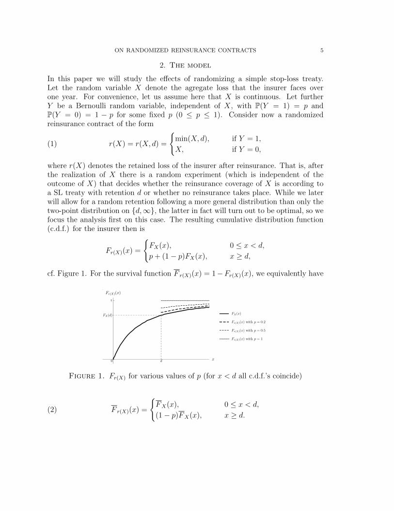
In this paper we will study the effects of randomizing a simple stop-loss treaty.Let the random variable X denote the agregate loss that the insurer faces overone year. For convenience, let us assume here that X is continuous. Let furtherY be a Bernoulli random variable, independent of X, with P(Y = 1) = p andP(Y = 0) = 1 − p for some fixed p (0 ≤ p ≤ 1). Consider now a randomizedreinsurance contract of the form

(1) r(X) = r(X, d) =

{min(X, d), if Y = 1,

X, if Y = 0,

where r(X) denotes the retained loss of the insurer after reinsurance. That is, afterthe realization of X there is a random experiment (which is independent of theoutcome of X) that decides whether the reinsurance coverage of X is according toa SL treaty with retention d or whether no reinsurance takes place. While we laterwill allow for a random retention following a more general distribution than only thetwo-point distribution on {d,∞}, the latter in fact will turn out to be optimal, so wefocus the analysis first on this case. The resulting cumulative distribution function(c.d.f.) for the insurer then is

Fr(X)(x) =

{FX(x), 0 ≤ x < d,

p+ (1− p)FX(x), x ≥ d,

cf. Figure 1. For the survival function F r(X)(x) = 1−Fr(X)(x), we equivalently have

Figure 1. Fr(X) for various values of p (for x < d all c.d.f.’s coincide)

(2) F r(X)(x) =

{FX(x), 0 ≤ x < d,

(1− p)FX(x), x ≥ d.


From the latter expression, one easily deduces the expected retained claim amount

E [r(X, d)] = E [X]− p∫ ∞d

FX(x)dx.

Let π(X) denote the total premium that the first-line insurer received from policy-holders for accepting the aggregate risk X. Following a suggestion of Kull [20], onecan consider the annual loss

Loss = X − π(X) + rCoC · ρ(Loss),

where rCoC ·ρ(Loss) reflects capital costs, with rCoC denoting a cost-of-capital rate andρ a solvency risk measure. For a positively homogeneous and translation-invariantrisk measure ρ, this leads to

ρ(Loss) =ρ(X)− π(X)

1− rCoC,

and consequently the annual profit (i.e. negative loss) is given by

(3)π(X)

1− rCoC−X − rCoC

1− rCoC· ρ(X)

(note that this approach for incorporating solvency capital requirements focuses onthe current-year insurance risk only, which could then be complemented by marketrisk, counterparty risk, multi-year loss development patterns etc., see [1, Ch.8] forfurther details). If a reinsurance treaty of the form (1) is entered for a premiumπR(d), then (3) changes into

(4) Z(d) =π(X)− πR(d)

1− rCoC− r(X, d)− rCoC

1− rCoC· ρ(r(X, d)).

As a performance measure of a reinsurance treaty, we will in this paper choosethe resulting expected annual profit E(Z(d)), since it combines the solvency aspectwith the profitability considerations in an intuitive way. Furthermore, to simplifycalculations we will assume an expected value principle for the reinsurance premium(with relative safety loading θ > 0):

πR(d) = (1 + θ)E [X − r(X, d)] = (1 + θ)p

∫ ∞d

FX(x)dx.

For the risk measure ρ, we choose the Value-at-Risk (VaR) at level 1 − α and usethe notation

ρ(X) = VaRα(X) = inf{x : FX(x) ≤ α}, α ∈ (0, 1).

This leads to the optimization problem


max0≤p≤1, d≥0

E [Z(d)](5)

with

E [Z(d)] =π(X)

1− rCoC− E [X]− rCoC

1− rCoC

((1 +

θ

rCoC

)p

∫ ∞d

FX(x)dx+ VaRα(r(X, d))

).

(6)

In view of (6), the optimization problem (5) can be reformulated as

g(d∗, p∗) := mind≥0, 0≤p≤1

g(d, p),(7)

where

g(d, p) :=

(1 +

θ

rCoC

)p

∫ ∞d

FX(x)dx+ VaRα(r(X, d)).(8)

Clearly, the trade-off to consider is to reduce the capital costs with a not too ex-pensive reinsurance premium, and we will see in the sequel that under the presentassumptions this trade-off can be more efficiently resolved introducing randomizedreinsurance forms, i.e. 0 < p < 1.

Remark 2.1. For general reinsurance treaties r(X), a general premium principle πRand risk measure ρ the above optimization criterion leads to minimizing

πR(X − r(X))− (1− rCoC)E [X − r(X)] + rCoC · ρ(r(X))

over all admissible r(X). Note that this in general differs from the purely risk-averseobjective function ρ(πR(X − r(X)) + r(X)) used by Cai & Tan [6] and several sub-sequent papers in the literature, but in case of the expected value premium principleand translation invariance of ρ the two can be identified for a modified value of thesafety loading coefficient (and hence different weighting), cf. [1, Sec.8.4] for details.

3. The optimization problem

In view of (8), it is clear that in our setting only retention values d < F−1

X (α) are ofinterest, as otherwise the reinsurance treaty does not improve VaRα(X) and thereforeit is better not to take reinsurance at all (and keep the saved reinsurance premiumfor profit). Whenever p > 0 is optimal, for each potentially optimal candidate

retention d < F−1

X (α), the optimal value of p has to be the one such that Fr(X,d)(d) =p+ (1− p)FX(d) = 1− α, i.e.

(9) p(d) = 1− α

FX(d),

cf. Figure 2.


Figure 2. Optimal value of p in a randomized stop-loss treaty

Indeed, if p + (1 − p)FX(d) > 1 − α, then the solvency capital requirement is over-fulfilled in the sense that the same level of VaRα(r(X, d)) could be achieved fora lower reinsurance premium simply by decreasing p to (9). On the other hand,for any p with p + (1 − p)FX(d) < 1 − α, one could attain the same level ofVaRα(r(X, d)) by increasing d (i.e. transferring the location of the jump of Fr(X,d))

to the level d > d such that p+ (1− p)FX(d) = 1− α holds, so that the same value

VaRα(r(X, d)) = VaRα(r(X, d)) = F−1

X

(α

1−p

)is achieved by a smaller reinsurance

premium. Consequently, the original d could not have been optimal for the overalloptimization problem. One can hence fix p(d) according to (9) and the optimizationproblem (7) reduces to the one-dimensional problem

min0≤d≤F−1

X (α)

g(d, 1− α/FX(d)).(10)

Note that if the optimal retention is the right-end point of this interval, i.e. d∗ =

F−1

X (α), the corresponding probability is p∗ = p(d∗) = 0, which means no reinsurance(this also corresponds to d =∞ for any p) and the resulting objective function then

is VaRα(X) = F−1

X (α).It is clear from (9), but useful to note for later purposes, that we always have p(d) ≤1− α, with equality for d = 0.


Problem (10) translates into

min0≤d≤F−1

X (α)

(1 + θ/rCoC) (1− α/FX(d))

∫ ∞d

FX(x)dx+ d.

This can also be expressed in terms of the mean-excess function eX(u) = E(X−u|X >u) and the pure reinsurance premium πSL(d) =

∫∞dFX(x)dx of a classical unbounded

stop-loss contract (i.e. p = 1):

min0≤d≤F−1

X (α)

(1 + θ/rCoC) (πSL(d)− α · eX(d)) + d.(11)

One observes that the shape of this function strongly depends on the distributionof the loss variable X and a general analysis is difficult. In any case, a particularcandidate for an optimal retention d is the solution of the equation

(12) (1 + θ/rCoC) (FX(d) + α · e′X(d)) = 1.

Example 3.1. If X is exponentially distributed with parameter ν, then eX(d) = 1/νand the solution of (12) is indeed

(13) d =1

νlog (1 + θ/rCoC) .

Since in this case F−1

X (α) = 1ν

log(1/α), the solution of the overall optimization

problem (5) is the following: If 1α> 1 + θ/rCoC, then the optimal retention d∗ is

given by (13) together with the corresponding p∗ = 1 − α (1 + θ/rCoC) (cf. (9)). If1α≤ 1 + θ/rCoC, then d∗ = ∞, i.e. no reinsurance of the form (1) should be taken

(in this case the reinsurance premium, through the loading θ, is too expensive or thecost-of-capital rate is too small relative to the solvency quantile α, so that reinsuranceis not efficient).

Example 3.2. If X follows a shifted Pareto distribution, i.e.

FX(x) = 1−(

ξ

x+ ξ

)1/γ

, ξ > 0 ; γ < 1,

then eX(d) = d+ξ1γ−1

, and the solution of (12) is given by

(14) d = ξ

((1

1 + θrCoC

− α1γ− 1

)−γ− 1

).


Since F−1X (α) = ξ (α−γ − 1), the solution of the overall optimization problem (5) is

as follows: If 1α

(1− γ) > 1 + θ/rCoC, then d∗ is given by (14) together with

p∗ =

1γ

(1− α

(1 + θ

rCoC

))− 1

1γ− α

(1 + θ

rCoC

)− 1

.

If 1α

(1− γ) ≤ 1 + θ/rCoC, then it is optimal to take no reinsurance.

Example 3.3. If X is uniformly distributed in [0, b], one has eX(d) = 1/2(b−d) ford < b, and

(15) d = b

(1−

(1

1 + θrCoC

+α

2

)),

solves (12). Because F−1X (α) = b(1 − α), the solution of the overall optimization

problem (5) then reads the following: If 2α> 1 + θ/rCoC, then d∗ is given by (15)

together with

p∗ =

11+ θ

rCoC

− α2

11+ θ

rCoC

+ α2

.

If 2α≤ 1 + θ/rCoC, then d∗ = ∞, i.e. the expected profit is maximized when no

reinsurance is purchased.

Remark 3.1. One could equivalently have started the analysis from the viewpointof choosing candidate values p first. Clearly, only p ≤ 1 − α can be optimal, sincethe resulting VaRα(r(X, d)) would not be improved by choosing p > 1 − α, whichis more expensive (note that in particular a classical unbounded stop-loss contract(p = 1) can not be optimal for (5), since reinsurance beyond the solvency quantile isnot efficient). In much the same way as above, one can now argue that the optimalchoice of d for a given p ≤ 1− α again has to fulfill p+ (1− p)FX(d) = 1− α, i.e.

(16) d(p) = F−1

X

(α

1− p

).

For any smaller (larger) d one can achieve the same VaR with a larger retention(smaller p, respectively) and hence a smaller premium in each case. Fixing (16), theoptimization problem (7) then reduces to the one-dimensional problem

min0≤p≤1−α

(1 +

θ

rCoC

)p

∫ ∞F

−1X ( α

1−p)FX(x)dx+ F

−1

X

(α

1− p

),(17)

which has a less intuitive form than (11). 2


In fact, the randomized treaty studied in this section (based on a two-point distribu-tion on {d,∞}) is the optimal treaty among all randomized stop-loss treaties witharbitrary distribution for the random retention:

Theorem 3.1. Let R be the set of all stop-loss treaties with a random retentionlevel D with c.d.f. FD, where D is independent of X. Assume that the reinsurancepremium is determined by πR(R) = (1+θ)E(R) for every R ∈ R. Then the expectedvalue of

E(π(X)− πR(X −R)

1− rCoC− (X −R)− rCoC

1− rCoC· VaRα(X −R)

)is maximized for

(18) D =

{d∗, with prob. p∗,

∞, with prob. 1− p∗.

Proof. Consider the optimal two-point solution (18). Since the reinsurance premiumfollows an expected value principle, it is proportional to the grey area in Figure 2.Whenever another random variable D leads to a different value of VaRα(X−R), thetwo-point distribution on {VaRα(X−R),∞} with the respective value p(VaRα(X−R)) according to (9) can generate the same VaR value, but for a cheaper reinsurancepremium. Hence the optimal choice of d∗ (together with p∗) can not be outperformedby any other random variable D that is independent of X. �

4. Optimizing the retention for fixed p

While the determination of the optimal pair (d∗, p∗) is already studied in Section 3,we now identify the optimal retention level for an arbitrary (possibly non-optimal)given probability level p. This will give some additional insight into the nature andconsequences of the randomization procedure. We will now also allow FX(0) > 0(which we refrained from in the previous sections for the sake of clarity of exposition,but which may for instance be relevant in some catastrophe insurance portfolios).Let us start with some general observations.

4.1. Preliminary properties. First, observe that if 1 − α ≤ FX(0), then clearlyVaRα(r(X, d)) = 0 for all d ≥ 0 in which case the expected profit in (5) is triviallymaximized for p = 0, i.e. no reinsurance. We hence assume α < FX(0) in thefollowing.

If 1 − α < FX(d), i.e. d > F−1

X (α), then VaRα(r(X, d)) = VaRα(X) = F−1

X (α).In this case the retention d exceeds the VaR of the original (and also the retained)risk, so reinsurance is again not of interest, as the reinsurance premium reduces the


expected profit, but does not lower the capital costs.

Next, for FX(d) ≤ 1 − α ≤ p + (1 − p)FX(d), i.e. (1 − p)FX(d) ≤ α ≤ FX(d), wehave VaRα(r(X, d)) = d.

Finally, in case 1−α > p+(1−p)FX(d), i.e. d < F−1

X

(α

1−p

), we have VaRα(r(X, d)) =

F−1

X

(α

1−p

).

Summarizing this differently, for each fixed retention d ≥ 0, the Value-at-Risk of theretained loss amount reads

(19) VaRα(r(X, d)) = F−1

X (α)

for p = 0,

(20) VaRα(r(X, d)) =

F−1

X

(α

1−p

), 0 ≤ d < F

−1

X

(α

1−p

),

d, F−1

X

(α

1−p

)≤ d ≤ F

−1

X (α),

F−1

X (α), d > F−1

X (α)

for p ∈(

0, 1− αFX(0)

), and

(21) VaRα(r(X, d)) =

{d, 0 ≤ d ≤ F

−1

X (α),

F−1

X (α), d > F−1

X (α)

for p ∈[1− α

FX(0), 1]. Note that in the latter case the Value-at-Risk is bounded by

d for any d ≥ 0 (cf. Figure 3 (right)), whereas it exceeds d in the range 0 ≤ d <

F−1

X

(α

1−p

)in the case p < 1 − α

FX(0)(cf. Figure 3 (left)). One observes that the

domain of the Value-at-Risk as a function of d is enlarged for increasing p, reachingthe situation on the right-hand picture when p tends to 1−α/FX(0) (and, conversely,

for p→ 0 the constant F−1

X (α) is reached for all values of d).


Figure 3. VaRα(r(X, d)) as a function of d for p < 1−α/FX(0) (left)and p ≥ 1− α/FX(0) (right).

The grey area depicted in Figure 4 represents all additional pairs (d,VaRα(r(X, d)))that can be obtained by varying p in the range p ∈

(0, 1− α/FX(0)

).

Figure 4. Effect of randomizing on the Value-at-Risk as a function of d

4.2. Optimization w.r.t. d for fixed p.

Proposition 4.1. Fix the value of p and let κ := 1p(1+θ/rCoC)

.

(i) Consider first the case p ≥ 1− α/FX(0). If

α < κ < FX(0)(22)

and

g(F−1

X (κ) , p)≤ F

−1

X (α),(23)

then a finite optimal retention d∗ exists and is given by

d∗ = F−1

X (κ) .


If

α < FX(0) ≤ κ

and

E [X] ≤ κF−1

X (α)

hold, then the finite optimal retention is d∗ = 0.(ii) For p ∈

(0, 1− α/FX(0)

), a finite optimal retention d∗ exists if

α < κ <α

1− p(24)

and

g(F−1

X (κ) , p)≤ F

−1

X (α),(25)

and then its value is also

d∗ = F−1

X (κ) .

Alternatively, if

κ ≥ α

1− p(26)

and

g

(F−1

X

(α

1− p

), p

)≤ F

−1

X (α),(27)

the optimal retention is given by

d∗ = F−1

X

(α

1− p

).

If none of the above conditions hold, d∗ =∞ (i.e. no reinsurance).

Proof. Let us first consider the case p ∈[1− α/FX(0), 1

]. Then,

(28) g(d) := g(d, p) =

{gL(d), 0 ≤ d ≤ F

−1

X (α),

gU(d), d > F−1

X (α)

with

gL(d) : =

(1 +

θ

rCoC

)p

∫ ∞d

FX(x)dx+ d,

gU(d) : =

(1 +

θ

rCoC

)p

∫ ∞d

FX(x)dx+ F−1

X (α).


Clearly, from (28), g(d) is continuous on d ∈ [0,∞) and tends to F−1

X (α) as d →∞. In addition, observe that for κ < FX(0), gL(d) is decreasing on

[0, F

−1

X (κ))

,

increasing on(F−1

X (κ),∞)

and attains a minimum at F−1

X (κ). Therefore, since

gU(d) is decreasing on d ∈ [0,∞), g(d) attains a global minimum at F−1

X (κ) if α <

κ < FX(0) and g(F−1

X (κ))≤ F

−1

X (α). Here, the latter condition ensures that a

finite global minimum of g(d) exists, namely that the expected profit E [Z(d)] can

be increased through reinsurance. In this case, the optimal retention is d∗ = F−1

X (κ).

The condition α < κ is necessary, otherwise F−1

X (κ) ≥ F−1

X (α) and g(d) is thendecreasing on d ∈ [0,∞) in which case a finite optimal retention d∗ does not exist(i.e. it would be preferable not to buy reinsurance from a profitability aspect). Notethat if κ ≥ FX(0), gL(d) attains its minimum at d = 0 and is increasing on d ∈ (0,∞).Consequently, because gU(d) is decreasing on d ∈ [0,∞), a finite optimal retention

exists if and only if g(0) =(

1 + θrCoC

)pE[X] ≤ F

−1

X (α) which can be rewritten as

E[X] ≤ κF−1

X (α). Hence, in this case, the optimal retention is d∗ = 0 meaning thatthe expected profit is maximized by passing the entire risk to the reinsurer.

Let us now examine the case p ∈(

0, 1− αFX(0)

), where

(29)

g(d) =

(

1 + θrCoC

)p∫∞dFX(x)dx+ F

−1

X

(α

1−p

), 0 ≤ d < F

−1

X

(α

1−p

),(

1 + θrCoC

)p∫∞dFX(x)dx+ d, F

−1

X

(α

1−p

)≤ d ≤ F

−1

X (α),(1 + θ

rCoC

)p∫∞dFX(x)dx+ F

−1

X (α), d > F−1

X (α).

Again, g(d) is continuous on d ∈ [0,∞) with the limiting value F−1

X (α) as d → ∞.

Furthermore, observe from (29) that g(d) is decreasing on d ∈[0, F

−1

X

(α

1−p

)). The

subsequent behavior of g(d) is determined by the relations between κ, α and p. More

precisely, if κ ≥ α1−p , gL(d) is increasing on d ∈

(F−1

X

(α

1−p

),∞)

, so is g(d) on

d ∈(F−1

X

(α

1−p

), F−1

X (α)]

. Hence, because gU(d) is decreasing on d ∈ [0,∞), a

finite optimal retention d∗ exists only if g(F−1

X

(α

1−p

))≤ F

−1

X (α). In this case, g(d)

attains a global minimum at F−1

X

(α

1−p

), which is the optimal retention. In the case

α < κ < α1−p , g(d) is decreasing on d ∈

[0, F

−1

X (κ))

, increasing on(F−1

X (κ), F−1

X (α)]

and then decreasing again towards F−1

X (α) as d → ∞. The function g(d) then


attains a global minimum value at F−1

X (κ) if g(F−1

X (κ))≤ F

−1

X (α). Hence, d∗ =

F−1

X (κ) is the optimal retention. Finally, if κ ≤ α, f(d) is decreasing on d ∈ [0,∞).Consequently, a finite optimal retention d∗ does not exist. �

5. Numerical illustrations

In this section, we illustrate the effects of the proposed randomized stop-loss treaty onthe expected profit and discuss some quantitative properties of the resulting optimalretention level d∗. Assume that the distribution function of the aggregate loss of theinsurer is given by

FX(x) =

{0.05, x = 0,

1− 0.95(

10001000+x

)3, x > 0,

i.e. a shifted Pareto distribution with an atom at 0. Furthermore, assume that thefirst-line insurance premium is determined by π(X) = (1 + 0.1) · E [X] = 522.5.

5.1. Optimal retention level d∗ as a function of p. Figure 5 depicts the optimalretention d∗ as a function of p for θ = 0.2, rCoC = 0.07 and α = 0.05. Recall fromSection 4.1 that one needs to distinguish the regions p ∈ (0, a) and p ∈ [a, 1] witha := 1 − α/FX(0) ≈ 0.947 for the analysis (indicated by the right vertical dashedline). In both cases, the existence and representation of the optimal retention d∗ iscontingent on the value of κ = κ(p) ≈ 0.259

p. For p ∈ (0, a), the two subcases κ ≥ α

1−pand α < κ < α

1−p have to be treated separately (see the left vertical dashed line

at p ≈ 0.838 for which κ = α1−p). In all these cases, the conditions of Proposition

4.1 are verified for the considered parameter set and any p ∈ (0, 1], so that a finiteoptimal retention level d∗ is known to exist. For p ∈ (0, 0.838] (i.e., κ ≥ α

1−p), the

optimal retention d∗ is given by F−1

X

(α

1−p

)and is decreasing in p. In this region, in

order to maximize the expected profit, it is optimal to choose d such that the VaRis minimized; the gains from a cheaper reinsurance premium with a larger retentionwould not offset the additional costs arising from a larger VaR. As p increases withinthis region, smaller VaR values can be attained (cf. Figure 4), explaining the decreasein the optimal retention d∗ up to p = 0.838. The rate of this decrease corresponds tothe rate at which the VaR domain is enlarged (as a function of d) when p increases.At p = 0.838, the savings on the reinsurance premium from choosing larger valuesof d start to dominate the capital costs for resulting higher VaR values. As a result,

the optimal retention given by d∗ = F−1

X (κ) increases on p ∈ (0.838, 1] with a smoothtransition through the right vertical line at p = 0.947.


Figure 6. Optimal retention d∗ as a function of p for θ = 0.11(dotted), θ = 0.15 (dashed) and θ = 0.2 (solid) with α = 0.05 andrCoC = 0.07.

Figure 5. Optimal retention d∗ as a function of p for θ = 0.2 (solid)with α = 0.05 and rCoC = 0.07.

Let us now examine the effects of the reinsurance loading θ on the optimal retentionlevel d∗. When reinsurance becomes cheaper, i.e. θ decreases, reinsurance premiumsavings are reduced. This has the effect of shifting the solution p of κ(p) = α

1−ptowards higher p-values, in the present case to 0.864 for θ = 0.15 and 0.886 forθ = 0.11. Since reinsurance premium savings become worth considering only forhigher p-values, minimizing the VaR is of interest in an extended region, resulting inan extended decrease of d∗ for smaller reinsurance loadings (cf. Figure 6).Note that θ and rCoC enter in κ as a ratio, so if both these parameters increase ordecrease to the same relative extent, the resulting shape of the optimal retention d∗

as a function of p will remain unchanged. Another observation is that the optimalretention d∗ is not affected by a change in the reinsurance premium loading up to


p = 0.838 for the considered θ-values (here, θ almost doubles form 0.11 to 0.2). Thereason is again the trade-off between VaR and reinsurance premium (and the factthe reinsurance premium is based on the expected value principle). In other words,if p is fixed at such (not too large) values, an increased reinsurance premium willstill lead to the same insurer’s preference choice of the retention. In order to furtherillustrate this point, Figure 7 depicts d∗ as a function of θ for a fixed value of p = 0.8.For all values of θ up to θ = 0.28 (which signifies the value for which κ(θ) = α

1−p), d∗

remains unchanged. Beyond that value, d∗ increases. Finally, for θ ≥ 0.449 condition(25) is not fulfilled any more, and reinsurance becomes too expensive for the insurerto enter a reinsurance agreement of this type at all.

Figure 7. Optimal retention d∗ as a function of θ for p = 0.8.

5.2. Optimal p∗ as a function of the retention d. For each given retention leveld ≥ 0, one can also look for the optimal p ∈ [0, 1] that maximizes the expected profit.Figure 6 depicts p∗ as a function of the retention level d for different reinsuranceloadings. Note that for small values of d and high reinsurance loading, it is preferableto have no reinsurance at all.


Figure 8. Optimal p∗ as a function of d for θ = 0.11 (dotted), θ = 0.2(dashed) and θ = 0.3 (solid).

5.3. Maximal expected profit as a function of p. Let us now analyze the impactof introducing randomness in the reinsurance treaty on the expected profit. Figure9 depicts the maximal expected profit (under the choice of the respective best d∗(p))as a function of p for various reinsurance loadings. It is interesting to observe thatalthough d∗ is first decreasing in p on κ ≥ α

1−p , the expected profit is first increasing

in p. Thus, having the possibility to choose a smaller VaR (by decreasing d∗) inresponse to an increase in p outbalances the increase in the reinsurance premium(through both an increase of p and decrease of d∗) in an increasing fashion. Themaximal expected profit is attained when the optimal pair (d∗, p∗) is chosen. In thepresent illustration p∗ is 0.863 for θ = 0.11, 0.829 for θ = 0.15 and 0.804 for θ = 0.18.As p approaches 1, the gains diminish again. Note that the randomized strategyoutperforms the classical deterministic stop-loss (p = 1) for a variety of p-values.One also sees that for higher reinsurance premiums (here θ = 0.15 and θ = 0.18),an over-all positive expected profit can only be achieved through randomization,not with a determinstic stop-loss contract (even when using the optimal retention).Figure 10 depicts the expected profit for arbitrary combinations of retentions d andprobabilities p.


Figure 9. Maximal expected profit E [Z(d∗)] as a function of p forθ = 0.11 (dotted), θ = 0.15 (dashed) and θ = 0.18 (black) with α =0.05 and rCoC = 0.07.

0

500

1000

1500d

0.0

0.5

1.0

p

-60

-40

-20

0

EHProfitL

Figure 10. Expected profit as a function of d and p.

Another interpretation is to see this as a stop-loss contract, the retention of which iseither ∞

6. Comparison with bounded stop-loss contracts

Randomization adds a degree of freedom to the classical stop-loss treaty, and so onemay argue that this naturally leads to an improved solution. From Figure 1 it be-comes clear that the resulting shape of the retained loss distribution of a randomizedstop-loss treaty resembles a deterministic bounded stop-loss treaty

(30) rB(X) = x−min{(X − dB)+, lB}


with retention dB and upper limit lB. It is hence particularly instructive to comparethe two. Note that beyond the retention the former takes a convex combination ofthe original loss c.d.f. FX and the constant 1, whereas the latter shifts the part ofFX to the right of dB + lB by lB units to the left, cf. Figure 11. Hence, even ford = dB, the resulting contracts will in general be different.

Figure 11. Original and retained loss distribution under randomizedreinsurance (1) (left) and the bounded stop-loss contract (30) (right)

In [11], it has been shown that a bounded stop-loss treaty minimizes the total re-tained risk exposure of an insurer within the class of deterministic reinsurance formswhere both the ceded and retained loss functions are non-decreasing. As outlinedin Remark 2.1, under the expected value principle for the reinsurance premium, thisthen also applies to the objective function used in the present paper, but underdifferent weights for the sum of the competing terms. We now want to comparethe optimal randomized strategy (d∗, p∗) with the optimal bounded stop-loss treaty(d∗B, l

∗B(d∗B)). By similar arguments as in Section 3 (or also following the reasoning

in [11]), it is clear that it is better not to take any reinsurance if d∗B ≥ F−1

X (α), and

in the other case necessarily l∗B(d∗B) = F−1

X (α)− d∗B. That is,

r∗B(x) =

{x−min

((x− d∗B)+, F

−1

X (α)− d∗B), if d∗B < F

−1

X (α),

x, if d∗B ≥ F−1

X (α),(31)

with d∗B = F−1

X

(1

1+θ/rCoC

). The analogue of (8) for the optimal bounded stop-loss

then is

gB(d∗B) :=

(

1 + θrCoC

) ∫ F−1X (α)

d∗BFX(x)dx+ d∗B, if d∗B < F

−1

X (α),

F−1

X (α), if d∗B ≥ F−1

X (α).(32)

For the best randomized stop-loss treaty, the respective amount reads

g

(d∗, 1− α

FX(d∗)

)=

{(1 + θ

rCoC

)(1− α

FX(d∗))∫∞d∗FX(x)dx+ d∗, if d∗ < F

−1

X (α),

F−1

X (α), if d∗ ≥ F−1

X (α),


where d∗ is determined according to Section 3.

Let us consider any candidate retention 0 ≤ d < F−1

X (α) and d = dB. Then for boththe randomized stop-loss and the bounded stop-loss, the choice p∗(d) and l∗B(d) willbe such that the resulting VaRα(r(X)) is equal to d. To quantify the performancedifference of the two treaties one is thus left with comparing the pure reinsurancepremiums:

h(d) : =

(1− α

FX(d)

)∫ ∞d

FX(x)dx−∫ F

−1X (α)

d

FX(x)dx,

=

∫ ∞F

−1X (α)

FX(x)dx− α · eX(d),

= α(eX

(F−1

X (α))− eX(d)

).

Correspondingly, if the mean-excess function is increasing, which is a property typ-ically shared by the class of heavy-tailed distributions (see e.g. Embrechts et al.[14, Ch.6]), it follows that a bounded stop-loss treaty is preferable to a randomizedstop-loss treaty for each fixed retention level d = dB. In other words, shifting thedistribution by l∗B(d) to obtain VaRα(r(X)) = d then leads to a cheaper premiumthan reshaping the c.d.f. by randomization towards VaRα(r(X)) = d. Since thisis true for all d, the best bounded stop-loss treaty then also outperforms the bestrandomized stop-loss treaty.On the other hand, for distributions with decreasing mean-excess function (like theuniform distribution, certain Gamma distributions or the light-tailed Weibull distri-bution), randomization outperforms bounded stop-loss for each retention level andcorrespondingly also for the respective optimal retention levels.When the mean-excess function is not monotone, the performance comparison canbe more intricate, cf. Example 6.4.

In the following, we consider some concrete examples.

Example 6.1. If X is exponentially distributed, the mean-excess function eX(d) is

constant, so that h(d) = 0 for all d < F−1

X (α). This means that in this case the bestrandomized stop-loss and the best bounded stop-loss treaty lead to the same resultingloss distribution, and correspondingly the optimal values d∗ and d∗B must coincide.This is of course due to the lack-of-memory property of the exponential distribution:for the region to the right of the retention level d, shifting the distribution functionfrom the right by l∗B(d) into the point (d, 1 − α) is equivalent to rescaling it up intothat same attachment point. This can also easily be verified analytically by realizing


that P(r(X, d) > d + y) = αP(X > y) as well as P(rB(X) > dB + y) = αP(X > y)for the respective optimal values p∗(d) and l∗B(dB) and all y > 0.

Example 6.2. Let X be uniformly distributed in [0, b], in which case F−1

X (α) =b(1 − α). Here eX(d) is decreasing in d, so a randomized stop-loss will lead to abetter profitability. The optimal bounded stop-loss is the following: If 1/α > 1 +

θ/rCoC, then the retention d∗B = b

(1− 1

1+ θrCoC

)is chosen together with the layer

l∗B(d∗B) = b

(1

1+ θrCoC

− α)

, otherwise it is preferable not to buy reinsurance. After

some calculations, one gets

gB(d∗B) =

b2

(−α2

(1 + θ

rCoC

)+

1+ 2θrCoC

1+ θrCoC

), if 1

α> 1 + θ

rCoC,

b(1− α), if 1α≤ 1 + θ

rCoC.

(33)

At the same time, under the optimal randomized stop-loss, we have in view of (15)

g (d∗, p∗) =

b(

1− 12

(α + 1

1+ θrCoC

)− 1

8α2(

1 + θrCoC

)), if 2

α> 1 + θ

rCoC,

b(1− α), if 2α≤ 1 + θ

rCoC.

(34)

The difference gB(d∗B)− g(d∗, p∗) := D reads

D =

0, if 1

α≤ 1

2

(1 + θ

rCoC

),

b2

(1

1+ θrCoC

+ α(α2

(1 + θ

rCoC

)− 1))

> 0, if 12

(1 + θ

rCoC

)< 1

α≤(

1 + θrCoC

),

bα2

(1− 3

4α(

1 + θrCoC

))> 0, if 1

α> 1 + θ

rCoC.

(35)

Correspondingly, the best randomized stop-loss treaty is always at least as good asthe best bounded stop-loss contract, and typically better. Note that the performancedifference increases in b. It is also worth mentioning that for a uniformly distributedrisk with a bounded stop-loss, the c.d.f. of the retained amount attains 1 at b−l∗B < b,which is sub-optimal in view of minimizing the reinsurance premium. Conversely, byconstruction, the resulting c.d.f. of randomized stop-loss attains 1 only at b. Figure12 illustrates the expected profit under the optimal bounded stop-loss (dashed) andthe optimal randomized stop-loss (solid) for α = 0.05, rCoC = 0.07 and b = 5 as afunction of the premium loading θ.


Figure 12. Expected profit with the optimal bounded stop-loss(dashed) vs. optimal randomized stop-loss (solid)

Example 6.3. Let X be a shifted Pareto random variable with

FX(x) = 1−(

ξ

x+ ξ

)1/γ

, ξ > 0 ; γ < 1.

In this case the mean-excess function eX(d) is increasing, so a randomized stop-losstreaty can not outperform the best bounded stop-loss. The optimal bounded stop-loss strategy is as follows: If 1/α > 1 + θ/rCoC, then one chooses the retention d∗B =

ξ

((1

1+ θrCoC

)−γ− 1

)together with the layer l∗B(d∗B) = ξ

(α−γ −

(1

1+ θrCoC

)−γ), oth-

erwise no reinsurance is taken. In view of (32), this translates into

gB(d∗B) :=

ξ((

11+ θ

rCoC

)−γ− 1 +

(1+ θ

rCoC

)1γ−1

((1

1+ θrCoC

)1−γ

− α1−γ

)), if 1

α> 1 + θ

rCoC,

ξ (α−γ − 1) , if 1α≤ 1 + θ

rCoC.

On the other hand, in view of (14), the optimal randomized stop-loss strategy is givenby

g (d∗, p∗) =

ξ((

1a− α

1γ−1

)−γ (1 + a

1γ−1

(1a− α

1−γ

))− 1

), if 1

α(1− γ) > a,

ξ (α−γ − 1) , if 1α

(1− γ) ≤ a,


where a := 1 + θrCoC

. The difference D := gB(d∗B)− g(d∗, 1− α

FX(d∗)

)then takes the

form

D =

0, if 1α≤ a,

ξ

(aγ − α−γ + a

1γ−1

(aγ−1 − α1−γ)

)< 0, if a < 1

α≤ a

1−γ ,

ξ

(( 1γ−1)(a

γ

γ−aα1−γ)+ 1

γ (1+aα− 1γ )(

1a− α

1γ−1

)−γ)

( 1γ−1)

2 < 0, if 1α> a

1−γ ,

(36)

so that indeed here a bounded stop-loss contract is always preferable.

Example 6.4. Let us now consider an example of a distribution with non-monotonemean-excess function. Concretely, let us introduce an upper truncation point T > 0to the shifted Pareto distribution considered in Example 6.3, i.e.

FX(x) =1−

(ξ

x+ξ

) 1γ

1−(

ξT+ξ

) 1γ

, 0 ≤ x ≤ T ; ξ > 0 ; γ < 1.

Such distributions recently gained some popularity in insurance claims modelling (seee.g. [1, Ch.4]). The corresponding mean-excess function is

eX(d) =

(ξ

T+ξ

) 1γ(d+ ξ + (T−d)

γ

)−(

ξd+ξ

) 1γ

(d+ ξ)(1γ− 1)((

ξT+ξ

) 1γ −

(ξd+ξ

) 1γ

) , 0 ≤ d < T,

which is non-monotone (first increasing and then decreasing to 0) for triples (ξ, γ, T )with e′X(0) > 0 (cf. Figure 13).


Figure 13. Possible shape of the mean-excess function for a shiftedtruncated Pareto random variable

Figure 14 depicts the expected profit under both treaties as a function of the truncationpoint T for ξ = 20, γ = 0.5, α = 0.05, θ = 0.2 and rCoC = 0.07. One sees that thereis a threshold value for T above which the heavy-tailed feature of the risk X starts todominate, making bounded stop-loss more attractive. However, for smaller values ofT the randomized stop-loss is preferable.

Figure 14. Expected profit with optimal bounded stop-loss (dashed)vs. optimal randomized stop-loss (solid) as a function of T

7. Conclusion

In this paper, we showed that randomizing classical reinsurance treaties can be bene-ficial for the insurer. While randomization is a well-known mathematical tool to helpidentifying optimal deterministic solutions, the purpose here was to initiate a discus-sion and ponder the possibilities of actually implementing additional randomness in


the settlement of the risk sharing arrangement between insurer and reinsurer. In thiscontext, one should keep in mind that randomization has potential advantages withrespect to moral hazard problems, as it is unclear during the settlement procedurewho will finally have to pay the claim. Also, when comparing the randomized stop-loss treaty with deterministic bounded stop-loss, one may argue that in the formercase the resulting retained loss distribution beyond the retention is determined bya part closer to the center for which one may have more confidence in the chosenmodel (as in the latter the respective part is further in the tail of the original lossdistribution).We deliberately chose a simple form of randomization as well as simple model assump-tions here, in order to make the reasoning transparent, and clearly many variantsand generalizations are possible. This includes considering more general reinsurancepremium principles, but also randomization of individual claims (like in excess-of-losstreaties). For instance, rather than participating with a fraction p in all claims likein a quota-share arrangement, the reinsurer could achieve a similar result by payingeach claim fully, but only with a probability p, independently for each claim (whichcan be preferable in terms of administrative expenses). On the aggregate level, onecan view the introduced randomization also as a simple alternative way to reshapethe loss distribution (for instance when ’picking’ any target point above the originalloss distribution function for the retained loss distribution function, one can realizethe resulting risk transfer through simple randomization. This can in general be asimple means to taylor the needs of clients for reinsurance companies (in terms oftarget shapes of the retained loss), and more intricate randomization mechanisms canfurther increase the possible variations. While the concept can seem non-intuitive inthe first place, it may provide a thought-provoking additional perspective on the na-ture of the problem (as well as on the choice of objective functions and constraints).In this paper, we focused on the Value-at-Risk for measuring risk, and the resultsdepend crucially on this choice. In a subsequent study, we will consider the effects ofrandomization for other choices of risk measures. However, the Value-at-Risk is therisk measure implemented in many regulatory systems nowadays, and the argumentsin this paper may underline some of the shortfalls of this risk measure (particularlythe encouragement to ’only’ optimize the retained situation up to the point of thesolvency requirement). Clearly, in practical situations the target solvency ratio willoften be considerably larger than 1, and corresponding adaptations of the argumentscan then be made.Finally, in this paper we considered the reinsurer’s preferences solely through thereinsurance premium rule. It will be interesting future work to include the rein-surer’s viewpoint on the suitability of randomized contracts by considering jointoptimization criteria.


Acknowledgements. We would like to thank Hans Buhlmann, Stefan Jaschke andLeonard Vincent for stimulating discussions on the topic.

References

[1] H. Albrecher, J. Beirlant, and J. Teugels. Reinsurance: Actuarial and Statistical Aspects. JohnWiley & Sons, Chichester, 2017.

[2] K. J. Arrow. Uncertainty and the welfare economics of medical care. 53(5):941–973, 1963.[3] S. Basak and A. Shapiro. Value-at-risk-based risk management: optimal policies and asset

prices. The Review of Financial Studies, 14(2):371–405, 2001.[4] C. Bernard and W. Tian. Optimal reinsurance arrangements under tail risk measures. Journal

of Risk and Insurance, 76(3):709–725, 2009.[5] K. Borch. An attempt to determine the optimum amount of stop loss reinsurance. Transactions

of the 16th International Congress of Actuaries, I(3):597–610, 1960.[6] J. Cai and K. S. Tan. Optimal retention for a stop-loss reinsurance under the VaR and CTE

risk measures. Astin Bull., 37(1):93–112, 2007.[7] J. Cai, K. S. Tan, C. Weng, and Y. Zhang. Optimal reinsurance under VaR and CTE risk

measures. Insurance: Math. Econom., 43(1):185–196, 2008.[8] K. C. Cheung. Optimal reinsurance revisited—a geometric approach. Astin Bull., 40(1):221–

239, 2010.[9] Y. Chi. Optimal reinsurance under variance related premium principles. Insurance: Math.

Econom., 51(2):310–321, 2012.[10] Y. Chi, X. S. Lin, and K. S. Tan. Optimal reinsurance under the risk-adjusted value of an

insurers liability and an economic reinsurance premium principle. North American ActuarialJournal, pages 1–16, 2017.

[11] Y. Chi and K. S. Tan. Optimal reinsurance under VaR and CVaR risk measures: a simplifiedapproach. Astin Bull., 41(2):487–509, 2011.

[12] Y. Chi and K. S. Tan. Optimal reinsurance with general premium principles. Insurance: Math.Econom., 52(2):180–189, 2013.

[13] C. L. Culp. Structured Finance and Insurance: The ART of Managing Capital and Risk. JohnWiley & Sons, 2011.

[14] P. Embrechts, C. Kluppelberg, and T. Mikosch. Modelling Extremal Events. Springer, Berlin,1997.

[15] L. Gajek and D. Zagrodny. Optimal reinsurance under general risk measures. Insurance Math.Econom., 34(2):227–240, 2004.

[16] L. Gajek and D. Zagrodny. Reinsurance arrangements maximizing insurer’s survival probabil-ity. Journal of Risk and Insurance, 71(3):421–435, 2004.

[17] M. Guerra and L. Centeno. Optimal reinsurance policy: The adjustment coefficient and theexpected utility criteria. Insurance Math. Econom., 42(2):529–539, 2008.

[18] M. Guerra and M. d. L. Centeno. Are quantile risk measures suitable for risk-transfer decisions?Insurance: Mathematics and Economics, 50(3):446–461, 2012.

[19] M. Kaluszka. Optimal reinsurance under mean-variance premium principles. Insurance Math.Econom., 28(1):61–67, 2001.

[20] A. Kull. Sharing risk – an economic perspective. Astin Bull., 39(2):591–613, 2009.[21] A. Lo. A Neyman-Pearson perspective on optimal reinsurance with constraints. ASTIN Bull.,

47(2):467–499, 2017.


[22] S. Malamud, H. Rui, and A. Whinston. Optimal reinsurance with multiple tranches. Journalof Mathematical Economics, 65:71–82, 2016.

[23] K. S. Tan, C. Weng, and Y. Zhang. VaR and CTE criteria for optimal quota-share and stop-lossreinsurance. North American Actuarial Journal, 13(4):459–482, 2009.

E-mail address: [email protected]

University of Lausanne and Swiss Finance Institute, Quartier UNIL-Dorigny, BatimentExtranef, 1015 Lausanne, Switzerland

E-mail address: [email protected]

University of Lausanne, Quartier UNIL-Dorigny, Batiment Extranef, 1015 Lau-sanne, Switzerland

on randomized reinsurance contracts - unil · reinsurance is a classical tool for the risk...

Documents