on optimal coarse spaces for domain decomposition and

On Optimal Coarse Spaces for DomainDecomposition and Their Approximation

Martin J. Gander, Laurence Halpern, and Kevin Santugini-Repiquet

1 Definition of the Optimal Coarse Space

We consider a general second order elliptic model problem

L u = f in Ω (1)

with some given boundary conditions that make the problem well posed. We decom-pose the domain Ω first into non-overlapping subdomains Ω j, j = 1,2, . . . ,J, andto consider also overlapping domain decomposition methods, we construct over-lapping subdomains Ω j from Ω j by simply enlarging them a bit. All domain de-composition methods provide at iteration n solutions un

j on the subdomains Ω j,j = 1,2, . . . ,J (or on Ω j in the case of overlapping methods, but then we just restrictthose to the non-overlapping decomposition Ω j to obtain an overall approximatesolution on which we base our coarse space construction). We want to study hereproperties of the correction that needs to be added to these subdomain solutionsin order to obtain the solution u of (1). This would be the best possible correction acoarse space can provide, independently of the domain decomposition method used,and it allows us to define an optimal coarse space, which we then approximate.

Since the unj are subdomain solutions, they satisfy equation (1) on their corre-

sponding subdomain,L un

j = f , in Ω j. (2)

Martin J. GanderUniversity of Geneva, Section of Mathematics, Rue du Lievre 2-4, CP 64, 1211 Geneva 4,Switzerland;e-mail: [email protected]

Laurence HalpernLAGA, Universite Paris 13, Avenue Jean Baptiste Clement, 93430 Villetaneuse, France; e-mail:[email protected]

Kevin Santugini-RepiquetBordeaux INP, IMB, UMR 5251, F-33400,Talence, France; e-mail: [email protected]

1

2 Martin J. Gander, Laurence Halpern, and Kevin Santugini-Repiquet

Defining the erroren

j(x) := u(x)−unj(x), x ∈ Ω j,

we see that the error satisfies the homogeneous problem in each subdomain,

L enj = 0 in Ω j. (3)

At the interface between the non-overlapping subdomains Ω j the error is in generalnot continuous, and also the normal derivative of the error is not continuous, sincethe subdomain solutions un

j in general do not have this property1. The best coarsespace, which we call optimal coarse space, must thus contain piecewise harmonicfunctions on Ω j to be able to represent the error.

2 Computing the Optimal Coarse Correction

Having identified the optimal coarse space, we need to explain a general methodto determine the optimal coarse correction in it. While two different approaches forspecific cases can be found in [8, 7], we present now a completely general approach:let us denote the interface between subdomain Ω j and Ωi by Γji, and let the jumpsin the Dirichlet and Neumann traces between subdomain solutions be denoted by

gnji(x) := un

j(x)−uni (x), hn

ji(x) := ∂n j unj(x)+∂niu

ni (x), x ∈ Γji, (4)

where ∂n j denotes the outer normal derivative of subdomain Ω j. Then the errorsatisfies the transmission problem

L enj = 0 in Ω j,

enj(x)− en

i (x) = gnji(x) on Γji,

∂n j enj(x)+∂nie

ni (x) = hn

ji(x) on Γji.(5)

Its solution lies in the optimal coarse space, and when added to the iterates unj , we

obtain the solution: the domain decomposition method has become a direct solver,it is nilpotent, independently of the domain decomposition method and the problemwe solve: no better coarse correction is possible!

We now give a weak formulation of the transmission problem (5). To simplifythe exposition, we use the case of the Laplacian, L := −∆ . We multiply the par-tial differential equation from (5) in each subdomain Ω j by a test function v j andintegrate by parts to obtain∫

Ω j

∇enj ·∇v j dx−∑

i

∫Γji

∂enj

∂n jv j ds = 0. (6)

1 For certain methods, continuity of the normal derivative is however assured, like in the FETImethods, or continuity of the Dirichlet traces, like in the Neumann-Neumann method or the alter-nating Schwarz method. This can be used to reduce the size of the optimal coarse space.

On Optimal Coarse Spaces for Domain Decomposition and Their Approximation 3

If we denote by en and v the functions defined on all of Ω by the piecewise definitionen|

Ω j:= en

j and v|Ω j

:= v j, then we can combine (6) over all subdomains Ω j to obtain

∫Ω

∇en ·∇vdx−∑j>i

∫Γji

(∂en

j

∂n jv j +

∂eni

∂nivi

)ds = 0. (7)

If we impose now continuity on the test functions v j, i.e. v to be continuous, then(7) becomes ∫

Ω


∫Γji

(∂en

j

∂n j+

∂eni

∂ni

)vds = 0, (8)

and we can use the data of the problem to remove the normal derivatives,∫Ω


∫Γji

hnjivds = 0. (9)

It is therefore natural to choose a continuous test function v to obtain a variationalformulation of the transmission problem (5), a function in the space

V := v : v|Ω j

=: v j ∈ H1(Ω j), v j = vi on Γji. (10)

Now the jump in the Dirichlet traces of the errors would in general be imposed onthe trial function space,

Un := u : u|Ω j

=: u j ∈ H1(Ω j), u j−ui = gnji on Γji, (11)

so the complete variational formulation for (5) is:

find en ∈Un, such that∫

Ω


∫Γji

hnjivds = 0 ∀v ∈V. (12)

To discretize the variational formulation (12), we have to choose approximationsof the spaces V and Un, and both spaces contain interior Dirichlet conditions. In afinite element setting, it is natural to enforce the homogeneous Dirichlet conditionsin Vh strongly if the mesh is matching at the interfaces, i.e. we just impose the nodalvalues to be the same for Vh.

While at the continuous level, the optimal coarse correction lies in an infinitedimensional space except for 1d problems, see [5, 7], at the discrete level this spacebecomes finite dimensional. It is in principle then possible to use the optimal coarsespace at the discrete level and to obtain a nilpotent method, i.e. a method whichconverges after the coarse correction, see for example [9, 8, 11, 10], and also [1]for conditions under which classical subdomain iterations can become nilpotent. Itis however not very practical to use these high dimensional optimal coarse spaces,and we are thus interested in approximations.


3 Approximations of the Optimal Coarse Space

We have seen that the optimal coarse space contains functions which satisfy the ho-mogeneous equation in each non-overlapping subdomain Ω j, i.e. they are harmonicin Ω j. To obtain an approximation of the optimal coarse space, it is therefore suf-ficient to define an approximation for the functions on the interfaces Γji, which arethen extended harmonically inside Ω j. A natural way to approximate the functionson the interfaces is to use a Sturm-Liuville eigenvalue problem, and then to selecteigenfunctions which correspond to modes on which the subdomain iteration of thedomain decomposition methods used is not effective. This can be done either forthe entire subdomain, for example choosing eigenfunctions of the Dirichlet to Neu-mann operator of the subdomain, see [2], or any other eigenvalue problem along theentire boundary of the subdomain Ω j, or piecewise on each interface Γji, in whichcase also basis functions relating cross points need be added [11, 10], see also theACMS coarse space [12] and references therein. This can be done solving for exam-ple lower dimensional counterparts of the original problem along the interface Γjiwith boundary conditions one at one end, and zero at the other, creating somethinglike hat functions around the crosspoint. Doing this for example for a rectangular do-main decomposed into rectangular subdomains for Laplace’s equation, this wouldjust generate Q1 functions on each subdomain. It is important however to not forcethese function to be continuous across subdomains, since they have to solve approx-imately the transmission problem (5) whose solution is not continuous, except forspecific methods2. So the resulting coarse basis function is not a hat function withone degree of freedom, but it is a discontinuous hat function with e.g. four degreesof freedom if four subdomains meet at that cross point.

Different approaches not based on approximating an optimal coarse space, butalso using eigenfunctions in the coarse space to improve specific inequalities in theconvergence analysis of domain decomposition methods are GenEO [14], whosefunctions are also harmonic in the interior of subdomains, and [3, 4], where volumeeigenfunctions are used which are thus not harmonic within subdomains. For a goodoverview, see [13].

4 Concrete Example: the Parallel Schwarz Method

We consider the high contrast diffusion problem ∇ · (a(x,y)∇u) = f in Ω = (0,1)2

with two subdomains Ω1 = (0, 1+δ

2 )× (0,1) and Ω2 = ( 1−δ

2 ,1)× (0,1). The classi-cal parallel Schwarz method is converging most slowly for low frequencies along theinterface x = 1

2 , i.e. error components represented in the Laplacian case by sin(kπy),k = 1,2, . . . ,K for some small integer K, see for example [6]. These are preciselythe eigenfunctions of the eigenvalue problem one obtains when using separation ofvariables, which in our high contrast case is

2 see footnote 1


1

0.5

00

0.5

0

1

0.5

1

1

0.5

00

0.5

0.5

1

0

1

1

0.5

00

0.5

0.5

1

0

1

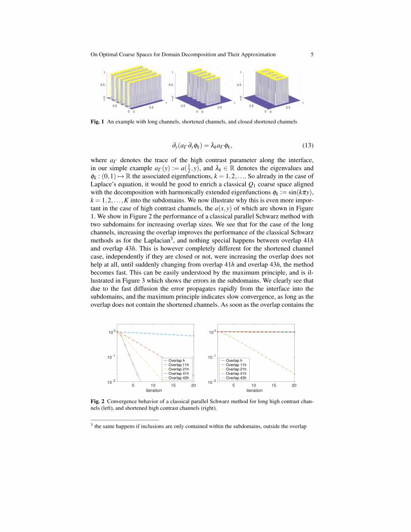
Fig. 1 An example with long channels, shortened channels, and closed shortened channels

∂y(aΓ ∂yφk) = λkaΓ φk, (13)

where aΓ denotes the trace of the high contrast parameter along the interface,in our simple example aΓ (y) := a( 1

2 ,y), and λk ∈ R denotes the eigenvalues andφk : (0,1) 7→ R the associated eigenfunctions, k = 1,2, . . .. So already in the case ofLaplace’s equation, it would be good to enrich a classical Q1 coarse space alignedwith the decomposition with harmonically extended eigenfunctions φk := sin(kπy),k = 1,2, . . . ,K into the subdomains. We now illustrate why this is even more impor-tant in the case of high contrast channels, the a(x,y) of which are shown in Figure1. We show in Figure 2 the performance of a classical parallel Schwarz method withtwo subdomains for increasing overlap sizes. We see that for the case of the longchannels, increasing the overlap improves the performance of the classical Schwarzmethods as for the Laplacian3, and nothing special happens between overlap 41hand overlap 43h. This is however completely different for the shortened channelcase, independently if they are closed or not, were increasing the overlap does nothelp at all, until suddenly changing from overlap 41h and overlap 43h, the methodbecomes fast. This can be easily understood by the maximum principle, and is il-lustrated in Figure 3 which shows the errors in the subdomains. We clearly see thatdue to the fast diffusion the error propagates rapidly from the interface into thesubdomains, and the maximum principle indicates slow convergence, as long as theoverlap does not contain the shortened channels. As soon as the overlap contains the

iteration5 10 15 20

10-2

10-1

100

Overlap hOverlap 11hOverlap 21hOverlap 41hOverlap 43h

iteration5 10 15 20

10-2

10-1

100

Overlap hOverlap 11hOverlap 21hOverlap 41hOverlap 43h

Fig. 2 Convergence behavior of a classical parallel Schwarz method for long high contrast chan-nels (left), and shortened high contrast channels (right).

3 the same happens if inclusions are only contained within the subdomains, outside the overlap


1

0.5

00

0.5

1

0.5

0

1

1

0.5

00

0.5

1

0.5

0

1

1

0.5

00

0.5

1

0.5

0

1

1

0.5

00

0.5

1

0.5

0

1

1

0.5

00

0.5

1

0.5

0

1

1

0.5

00

0.5

1

0.5

0

1

1

0.5

00

0.5

1

0.5

0

1

1

0.5

00

0.5

0

1

0.5

1

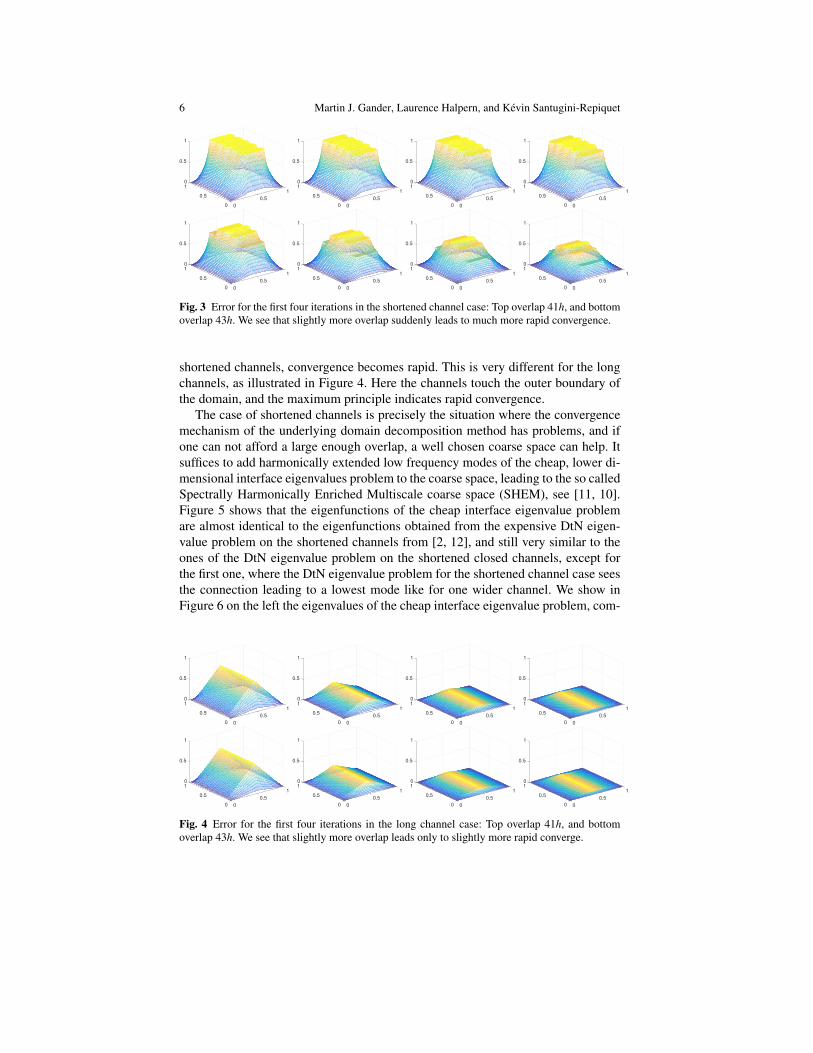
Fig. 3 Error for the first four iterations in the shortened channel case: Top overlap 41h, and bottomoverlap 43h. We see that slightly more overlap suddenly leads to much more rapid convergence.

shortened channels, convergence becomes rapid. This is very different for the longchannels, as illustrated in Figure 4. Here the channels touch the outer boundary ofthe domain, and the maximum principle indicates rapid convergence.

The case of shortened channels is precisely the situation where the convergencemechanism of the underlying domain decomposition method has problems, and ifone can not afford a large enough overlap, a well chosen coarse space can help. Itsuffices to add harmonically extended low frequency modes of the cheap, lower di-mensional interface eigenvalues problem to the coarse space, leading to the so calledSpectrally Harmonically Enriched Multiscale coarse space (SHEM), see [11, 10].Figure 5 shows that the eigenfunctions of the cheap interface eigenvalue problemare almost identical to the eigenfunctions obtained from the expensive DtN eigen-value problem on the shortened channels from [2, 12], and still very similar to theones of the DtN eigenvalue problem on the shortened closed channels, except forthe first one, where the DtN eigenvalue problem for the shortened channel case seesthe connection leading to a lowest mode like for one wider channel. We show inFigure 6 on the left the eigenvalues of the cheap interface eigenvalue problem, com-

1

0.5

00

0.5

1

0.5

0

1

1

0.5

00

0.5

1

0.5

0

1

1

0.5

00

0.5

1

0.5

0

1

1

0.5

00

0.5

1

0.5

0

1

1

0.5

00

0.5

1

0.5

0

1

1

0.5

00

0.5

1

0.5

0

1

1

0.5

00

0.5

1

0.5

0

1

1

0.5

00

0.5

1

0.5

0

1

Fig. 4 Error for the first four iterations in the long channel case: Top overlap 41h, and bottomoverlap 43h. We see that slightly more overlap leads only to slightly more rapid converge.


x0 0.5 1

0

0.05

0.1

Interface EVPDtN EVP Short OpenDtN EVP Short Closed

x0 0.5 1

-0.15

-0.1

-0.05

0

0.05

0.1

0.15


x0 0.5 1

-0.2

-0.1

0

0.1

0.2


x0 0.5 1

-0.2

-0.1

0

0.1

0.2


x0 0.5 1

-0.2

-0.1

0

0.1

0.2


x0 0.5 1

-0.4

-0.2

0

0.2

0.4


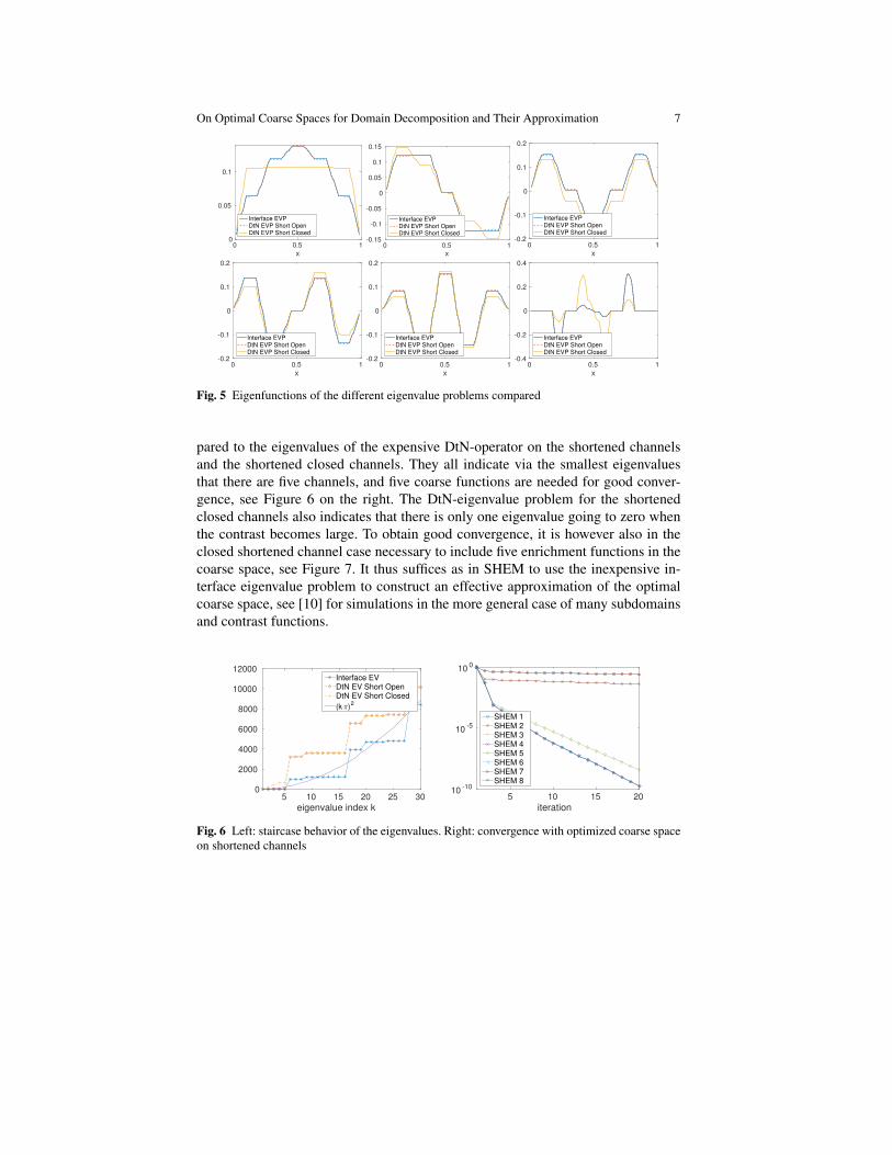
Fig. 5 Eigenfunctions of the different eigenvalue problems compared

pared to the eigenvalues of the expensive DtN-operator on the shortened channelsand the shortened closed channels. They all indicate via the smallest eigenvaluesthat there are five channels, and five coarse functions are needed for good conver-gence, see Figure 6 on the right. The DtN-eigenvalue problem for the shortenedclosed channels also indicates that there is only one eigenvalue going to zero whenthe contrast becomes large. To obtain good convergence, it is however also in theclosed shortened channel case necessary to include five enrichment functions in thecoarse space, see Figure 7. It thus suffices as in SHEM to use the inexpensive in-terface eigenvalue problem to construct an effective approximation of the optimalcoarse space, see [10] for simulations in the more general case of many subdomainsand contrast functions.

eigenvalue index k5 10 15 20 25 30

0

2000

4000

6000

8000

10000

12000Interface EVDtN EV Short OpenDtN EV Short Closed

(kπ)2

iteration

5 10 15 2010

-10

10-5

100

SHEM 1

SHEM 2

SHEM 3

SHEM 4

SHEM 5

SHEM 6

SHEM 7

SHEM 8

Fig. 6 Left: staircase behavior of the eigenvalues. Right: convergence with optimized coarse spaceon shortened channels


iteration

10 20 30 40

10-5

100

1 Coarse

2 Coarse

3 Coarse

4 Coarse

5 Coarse

6 Coarse

7 Coarse

8 Coarse

iteration

10 20 30 40

10-5

100

1 Coarse

2 Coarse

3 Coarse

4 Coarse

5 Coarse

6 Coarse

7 Coarse

8 Coarse

Fig. 7 Shortened closed channels problem. Left: coarse space based on the cheap interface eigen-value problem. Right: coarse space based on the expensive DtN eigenvalue problem which seesthe exact structure inside the subdomain, i.e. the shortened closed channels. Note that the perfor-mance is essentially the same: in both cases one needs 5 or more enrichment functions to get goodconvergence.

5 Conclusions

We introduced the concept of optimal coarse spaces for general elliptic problemsand domain decomposition methods with and without overlap, i.e. coarse spaceswhich lead to convergence in one iteration. We then gave a variational formula-tion for the associated coarse problem that needs to be solved in each iteration. Wealso explained how to approximate this coarse problem, by employing coarse spacecomponents for which the underlying domain decomposition method exhibits slowconvergence, and illustrated this approach with a high contrast problem containingchannels. The main advantage of our construction is that it is not based on a conver-gence analysis, but on the domain decomposition iteration itself, and can thus alsobe applied to methods where general convergence analyses are not yet available,like for example RAS [8, 10] and optimized Schwarz methods [7].

References

1. Faycal Chaouqui, Martin J. Gander, and Kevin Santugini-Repiquet. On nilpotent subdomainiterations. Domain Decomposition Methods in Science and Engineering XXIII, Springer,2016.

2. Victorita Dolean, Frederic Nataf, Robert Scheichl, and Nicole Spillane. Analysis of a two-level Schwarz method with coarse spaces based on local Dirichlet-to-Neumann maps. Comput.Methods Appl. Math., 12(4):391–414, 2012.

3. Juan Galvis and Yalchin Efendiev. Domain decomposition preconditioners for multiscaleflows in high-contrast media. Multiscale Model. Simul., 8(4):1461–1483, 2010.

4. Juan Galvis and Yalchin Efendiev. Domain decomposition preconditioners for multiscaleflows in high contrast media: reduced dimension coarse spaces. Multiscale Model. Simul.,8(5):1621–1644, 2010.

5. M Gander and Laurence Halpern. Methode de decomposition de domaine. Encyclopedieelectronique pour les ingenieurs, 2012.


6. Martin J. Gander. Optimized Schwarz methods. SIAM Journal on Numerical Analysis,44(2):699–731, 2006.

7. Martin J. Gander, Laurence Halpern, and Kevin Santugini-Repiquet. Discontinuous coarsespaces for DD-methods with discontinuous iterates. In Domain Decomposition Methods inScience and Engineering XXI, pages 607–615. Springer, 2014.

8. Martin J. Gander, Laurence Halpern, and Kevin Santugini-Repiquet. A new coarse grid cor-rection for RAS/AS. In Domain Decomposition Methods in Science and Engineering XXI,pages 275–283. Springer, 2014.

9. Martin J Gander and Felix Kwok. Optimal interface conditions for an arbitrary decompositioninto subdomains. In Domain Decomposition Methods in Science and Engineering XIX, pages101–108. Springer, 2011.

10. Martin J. Gander and Atle Loneland. SHEM: An optimal coarse space for RAS and its mul-tiscale approximation. Domain Decomposition Methods in Science and Engineering XXIII,Springer, pages 313–321, 2016.

11. Martin J. Gander, Atle Loneland, and Talal Rahman. Analysis of a new harmonicallyenriched multiscale coarse space for domain decomposition methods. arXiv preprintarXiv:1512.05285, 2015.

12. A. Heinlein, A. Klawonn, J. Knepper, and O. Rheinbach. Multiscale coarse spaces for over-lapping Schwarz methods based on the ACMS space in 2d. submitted to ETNA, 2017.

13. Robert Scheichl. Robust coarsening in multiscale PDEs. In Randolph Bank, Michael Holst,Olof Widlund, and Jinchao Xu, editors, Domain Decomposition Methods in Science and En-gineering XX, volume 91 of Lecture Notes in Computational Science and Engineering, pages51–62. Springer Berlin Heidelberg, 2013.

14. N. Spillane, V. Dolean, P. Hauret, F. Nataf, C. Pechstein, and R. Scheichl. Abstract robustcoarse spaces for systems of PDEs via generalized eigenproblems in the overlaps. Numer.Math., 126(4):741–770, 2014.

on optimal coarse spaces for domain decomposition and

Documents