molecular decomposition of the modulation spaces

Kobayashi, M. and Sawano, Y.Osaka J. Math.47 (2010), 1029–1053

MOLECULAR DECOMPOSITIONOF THE MODULATION SPACES

MASAHARU KOBAYASHI and YOSHIHIRO SAWANO

(Received September 20, 2007, revised July 1, 2009)

AbstractThe aim of this paper is to develop a theory of decomposition in the weighted

modulation spacesMs,Wp,q with 0 < p, q � 1, s 2 R and W 2 A1, where W be-

longs to the class ofA1 defined by Muckenhoupt. For this purpose we shall definemolecules for the modulation spaces. As an application we give a simple proof ofthe boundedness of the pseudo-differential operators withsymbols in M01,min(1,p,q).We shall deal with dual spaces as well.

1. Introduction

The modulation spaces, introduced by Feichtinger in 1983 (see [6]), are one ofthe function spaces to investigate growth, decay and regularity of functions or dis-tributions in a way other than the Besov spaces. Several important properties of themodulation spaces such as duality, interpolation theory and atomic decomposition werewell investigated by Feichtinger and Gröchenig [6, 7, 8, 9, 10]. Now they are recog-nized as appropriate function spaces and they are applied totime-frequency analysisand pseudo-differential calculus. For example, by using the theory of the modulationspaces, Sjöstrand and Tachizawa generalized the theory of Calderón–Vaillancourt [4, 25](see also the work due to Gröchenig–Heil [16]). In recent years, they are also appliedto study the global well-posedness of solutions for the Cauchy problem such as KdVand NLS equations [2, 3].

Based on the standard notation of signal analysis, we adopt the following notations.

Ta f (x) WD f (x � a), Mb f (x) WD eib �x f (x), a, b 2 Rn, f 2 S 0,f � g(x) WD ZRn

f (x � y)g(y) dy,

F f (� ) WD 1

(2�)n=2ZRn

f (x) exp(�i x � � ) dx,

F�1 f (x) WD 1

(2�)n=2ZRn

f (� ) exp(i x � � ) d� .

2000 Mathematics Subject Classification. Primary 42B35; Secondary 41A17.

1030 M. KOBAYASHI AND Y. SAWANO

To denote cubes inRn, we use

Q(r ) WD fx 2 Rn W max(jx1j, : : : , jxnj) � r g,Ql WD [l1, l1C 1] � [l2, l2C 1] � � � � � [ln, ln C 1]

for r > 0 and l 2 Zn. It will be helpful to use the notation from [28]. Letf 2 S 0 and� 2 S. Then we write

(1) � (D) f WD F�1(� � F f ) D (2�)�n=2F�1� � f .

As for the Fourier multipliers and the multiplication operators we prefer to avoid super-fluous brackets. We shall list some typical examples in this paper: Leta, b 2 Rn. Thenwe write Ta�(D) f WD [Ta�](D) f , Mb�(D) f WD [Mb�](D) f , Mb � f WD [Mb ] � f .If possible confusion can occur, we bind the function on which the operator acts.

Fix g 2 S n f0g. Then define

k f W Msp,qk WD

�ZRn

�ZRn

jh f , MyTxgijp dx

�q=p

(1C jyj)sq dy

�1=q

for s 2 R and 1� p, q � 1. Denote byMsp,q the set of all tempered distributions

f 2 S 0 for which the norm is finite. An important observation is thatthe function spaceMs

p,q does not depend on the specific choices ofg 2 S(Rn) n f0g. For more details werefer to [12].

In the present paper we consider the weighted modulation spaces. In general by aweighted modulation norm we mean the following norm given by

k f W Mvp,qk WD

�ZRn

�ZRn

jh f , MyTxgijpv(x, y) dx

�q=p

dy

�1=q.

Note thatMsp,q is recovered by settingv(x, y) D (1Cjyj)sq. There are many important

classes of weights.1. A weight v W R2n ! [0,1) is said to be a submultiplicative, if there exists a con-stantC > 0 such thatv(x C y) � Cv(x)v(y) for all x, y 2 R2n.2. Fix a submultiplicative weightv. A weight m is said to bev-moderate, if thereexists a constantC > 0 such thatm(x C y) � Cv(x)m(y) for all x, y 2 R2n.3. A weight is said to be subconvolutive, ifv�1 2 L1(R2n) and v�1 � v�1 � cv�1 forsome constantc > 0.4. A weight v is said to satisfy the Gelfand–Raikov–Shilov condition (respectivelythe Beurling–Domar condition, the logarithmic integral condition), if

limn!1 v(nx)1=n D 1 (resp.

P1jD1 log v(nx)=n <1,

Rjxj�1 log v(x)=jxjnC1 dx <1).

It is shown in [15] that the Beurling–Domar condition implies the Gelfand–Raikov–Shilov condition. We refer to [8] for more details of the submultiplicative, moderate

MOLECULAR DECOMPOSITION OF THEMODULATION SPACES 1031

and subconvolutive weights not only onRn but also on locally compact abelian groups.In the present paper, we consider weights of the form

v(x, y) D W(x)(1C jyj)s,

wheres2 R and W belongs to the classA1 of Muckenhoupt. As the exampleW(x)Djxj�, � > �n shows, it can happen thatv fails the submultiplicative condition or thesubconvolutive condition. Another similar example shows that v does not necessarilysatisfy the Beurling–Domar condition.

Before we go further, we recall the definition ofAp-weights. In the sequel by a“weight”, we mean a non-negative measurable functionW 2 L1

loc satisfying 0< W <1 for a.e. and we define the maximal operatorM by

M f (x) WD supx2Q

Q W cube

1jQjZ

Qj f (y)j dy.

Let 1� p <1. Then we define

Ap(W) D8��<��:

ess. supx2Rn

MW(x)

W(x)if p D 1,

supQ W cube

�1jQjZ

QW(x) dx

� �� 1jQjZ

QW(x)1=(1�p) dx

�p�1

if 1 < p <1.

The quantity Ap(W) is called theAp-norm of W, although Ap(W) is not actually anorm (see [20, 21]). Then it is easy to see that

Ap(W) � Aq(W), 1� q � p <1.

The classAp of weights is the set of all weightsW for which the normAp(W) isfinite. We also define

A1 WD [1�p<1 Ap.

We remark thatjxj�nC" 2 A1 for all 0< " < n. If W 2 A1, then we have

(2)Z

Q(l )W(x) dx � chl iM , l 2 Zn

for someM > 0 andc > 0.Let W be a weight. Then we define

k f W LWp k WD

�ZRn

j f (x)jpW(x) dx

�1=p

, 1� p <1.


Let 1< p < 1. Muckenhoupt showed that the maximal operatorM is bounded onLW

p if and only if W 2 Ap. Muckenhoupt also proved that the weak-(1, 1) estimate,that is, Z

fM f>�g W(x) dx � C�Z j f (x)jW(x) dx

holds if and only if W 2 A1. We refer to [20, 21] for more details.Having set down the elementary facts on the weights, let us describe the weighted

function spaceMs,Wp,q . Let 0< p, q � 1 and s 2 R. The first author of the present

paper noticed that the definition of the unweighted modulation spaces can be describedas follows: Pick a function� 2 S so that supp(�) � Q(2),

Pm2Zn Tm�(x) � 1 and

write hxi WDp1C jxj2. In [18] we have defined

(3) k f W Msp,qk WD

Xm2Zn

hmiqsk[F�1Tm�] � f W L pkq!1=q

for f 2 S 0. It is still possible to establish that different choices of� will give us anequivalent norm.

The main results of this paper can be summarized as follows: Most of the theoryof the modulation spacesMs

p,q carries over to theA1-weighted cases with 0< p, q �1 and s 2 R.Let W 2 A1 throughout. Then definek fm W lq(LW

p )k WD �Pm2Znk fm W LWp kq�1=q for

a family of measurable functionsf fmgm2Zn . Let 0< p, q � 1 and s 2 R. Then themodulation norm is given by

(4)

k f W Ms,Wp,q k WD khmisTm�(D) f W lq(LW

p )kD X

m2Zn

hmiqsk[F�1Tm�] � f W LWp kq

!1=q.

Here and below we assume thatW 2 AP with 1 � P <1 for the sake of defin-iteness.

A fundamental technique in harmonic analysis is to represent a function or dis-tribution as a linear combination of functions of an elementary form. We shall inves-tigate the structure of weighted modulation spaces and discuss several applications ofthis technique. For example, the “Gabor expansion” for the modulation spaces is dis-cussed in Gröchenig [12] and Galperin–Samarah [11]. The heart of the matter of thisexpansion is to decompose a function into a linear combination of elements of the fam-ily fTl MmggmI l2Zn which is created by just one “atomic” functiong. However, suchatomic decomposition has some disadvantages in analyzing the pseudo-differential op-erators. In general, it is not the case that the pseudo-differential operators map the


family fTl MmggmI l2Zn to another one created by an atomic function again. To over-come this disadvantage, we introduce the “molecular” decomposition. Molecules aremapped to molecules again by pseudo-differential operators (Lemma 3.2). We refer to[1, 17] for the definition of the molecules for different modulation spaces.

DEFINITION 1.1 (Molecule). Lets2 R. Suppose thatK , N 2 N are large enoughand fixed. ACK -function � W Rn ! C is said to be an (sIm, l )-molecule, if it satisfies

j��(e�im�x� (x))j � hmi�shx � l i�N , x 2 Rn

for j�j � K . Also set

Ms WD(

M D fmolsmlgm,l2Zn �CK W there existsc>0 such that

c �molsml is an (sIm, l )-molecule for everym, l 2Zn

).

The integersK and N are taken sufficiently large, say,K , N � 10[n=min(1, p=P,q)]CMC10, where [a] denotes the integer part ofa 2 R and M is a positive numberappearing in (2).

Next, we introduce a sequence spacemWp,q to describe the condition of the co-

efficients of the molecular decomposition.

DEFINITION 1.2 (Sequence spacemWp,q). Let 0< p, q�1. Given�D f�mlgm,l2Zn ,

define

k� W mWp,qk WD

(X

l2Zn

�ml�Ql

)m

W lq(LWp )

.

Here a natural modification is made whenp and/orq is infinite. The sequencemWp,q is

the set of doubly indexed sequences�D f�mlgm,l2Zn for which the quasi-normk� WmWp,qk

is finite.

With these definitions in mind, we shall present our main theorem in this paper.

Theorem 1.3. Let 0< p, q � 1 and s2 R. Let � 2 S be taken so that�Q(3) �� Q(3C1=100).1. Set molsml WD hmi�sTl Mm[F�1�]. The decomposition, called Gabor decomposition,holds for Ms,W

p,q . More precisely, we havefmolsmlgm,l2Zn 2Ms and the mapping

f 2 Ms,Wp,q 7! � D fhmisTm�(D) f (l )gm,l2Zn 2 mW

p,q

is bounded. Furthermore, any f 2 Ms,Wp,q admits the following Gabor decomposition

(5) f D Xm,l2Zn

�ml �molsml , � D f�mlgm,l2Zn D fhmisTm�(D) f (l )gm,l2Zn 2 mWp,q.


2. Suppose we are given MD fmolsmlgm,l2Zn 2Ms and � D f�mlgm,l2Zn 2 mWp,q. Then

(6) f WD Xm,l2Zn

�ml �molsml

converges unconditionally in the topology ofS 0. Furthermore f belongs to Ms,Wp,q and

satisfies the quasi-norm estimatek f W Ms,Wp,q k � Ck� WmW

p,qk. In particular if 0< p,q <1, then the convergence of(6) takes place in Ms,Wp,q .

In [11] Galperin and Samarah obtained the following result.

Theorem 1.4. Let 0 < p, q � 1 and f 2 S 0. Assume that� W R2n � R2n ! Ris submultiplicative. Assume in addition that mW R2n � R2n ! R is �-moderate. Fixg 2 S(Rn) n f0g and let �, � > 0 be sufficiently small.

Then f satisfies

�ZRn

�ZRn

jh f , MxT!gijpm(x, !)p dx

�q=p

d!�1=q <1if and only if f satisfies

Xm2Zn

Xk2Zn

jh f , Mm�Tk�gijpm(�m, �k)p

!q=p!1=q<1.

If this is the case, f admits the decomposition(5) in Theorem 1.3.

We remark that the part 1 of Theorem 1.3 is contained in Theorem 1.4 in theframework of the weighted setting ifw � 1 and m � 1. Note that the result in The-orem 1.4 does not cover our result whenw(x) D jxj�nC" for 0< " < n. But the maincontribution of this paper is the part 2 of Theorem 1.3, whichhas never explicitly ap-peared in any literature at least for our class of weight functions. This result is im-portant because pseudo-differential operators do not mapmolsml D hmi�sTl MmF� to afunction of the same form. All we can say is that the mapped onebelongs toMs

(Lemma 3.2). In other words, pseudo-differential operators map the functionf withthe decomposition (5) to another one with the decomposition(6). We can, however,recover the norm of the mapped function by virtue of Theorem 1.3 2. Actually wetake this advantage to show some boundedness result of pseudodifferential operators(Theorem 3.4).

Finally we describe the organization of this paper. In the next section, which isthe heart of this paper, we investigate the molecular decomposition of the modulationspaces. In Section 2, we prove our main result Theorem 1.3. Although the proof of thedecomposition result part 1 is just a suitable modification of the argument in [11], we


include it for reader’s convenience. Our main concern is, however, the proof of the syn-thesis result part 2. In Section 3 we investigate the pseudo-differential operators whosesymbol belongs toS0

0,0. Recall that a symbol classSm�,Æ with m 2 R and 0� �, Æ � 1

is the set ofC1(Rn�Rn)-functionsa satisfyingj��x �� a(x, � )j � C�,�h�im��j�jCÆj�j. We

remark thatM0p,q-boundedness of the pseudo-differential operators with symbols in the

Hörmander classSm�,Æ was obtained in [11, 16, 25] with 1� p, q � 1. As an applica-

tion of Ms,Wp,q -boundedness of this result and the decomposition result inSection 2 we

shall prove that the pseudo-differential operator with symbols in M01,min(1,p,q)(Rn�Rn)

is bounded onM0,Wp,q . We remark that in [12, 16] Gröchenig and Heil proved this re-

sult in the case when 1� p, q � 1. Recently there are many literatures proving theboundedness on the modulation spaces of the pseudo-differential operators with sym-bols in the Sjöstrand class (see [12, 17, 22]). In particularGröchenig established thistype of boundedness by using the almost-diagonization. Here we shall use our decom-position results directly. What is new about this result is the fact that we have provedthe counterpart for general parameters 0< p, q �1 and theA1-weighted setting, andthe point that we do not have to rely on the dual argument. We refer to [23, 24] fornon-negative results on the boundedness of the pseudo-differential operators. In Sec-tion 4 we exhibit another application of the results in Section 2. In [19] the first authorinvestigated the dual space ofM0

p,q with 0< p, q <1. However, the definitive resultwhen 0< p� 1� q <1 was missing. We exploit the molecular decomposition alongwith the method used in [5]. In the present paper we shall supplement this missingpart. The proof is again based on the molecular decomposition obtained in Section 2.

2. Molecular decomposition in Ms,Wp,q

In this section we deal with the molecular decomposition, inparticular, the syn-thesis property. We assume that� 2 S is a positive function satisfying

(7) supp(�) � Q(2),Xm2Zn

Tm�(x) � 1.

As preliminaries we collect two important results on the band-limited distributions.

Lemma 2.1 ([27, Chapter 1]). Let 0< � <1. Then there exists c> 0 such that

supy2Rnhyi�n=�j f (x � y)j � cM(�) f (x)

for all f 2 S 0 with diam(supp(F f )) � 10, where M(�) is a powered maximal operator:

(8) M (�) f (x) WD supx2Q

Q W cube

�1jQjZ

Qj f (y)j� dy

�1=�.


We note that under our notation the well-known maximal inequality reads

(9) kM (�) f W LWp k � ck f W LW

p k, 0< � < p � 1.

Let M 2 N. Denote byWM2 the Sobolev space consisting off 2 L2 satisfying

k f W WM2 k WD kh�iM � F f W L2k <1.

The following is a slight modification of the result in [27, Chapter 1].

Lemma 2.2 ([27, Chapter 1]). Let W 2 AP with 1 � P < 1. Let 0 < p � 1and M 2 N with M > n=min(1, p=P) � n=2. Set

H (D) f (x) WD (2�)�n=2 ZRn

H (� )F f (� )ei x �� d�for H 2 S and f 2 S 0. Then there exists a constant c> 0 independent of R> 0 so that

kH (D) f W LWp k � ckH (R � ) W WM

2 k � k f W LWp k,

whenever H2 WM2 and f 2 LW

p \ S 0 with diam(supp(F f )) � R.

From this lemma we can easily deduce that the definition of thefunction spaceMs,W

p,q does not depend on the choice of� 2 S satisfying (7).The following well-known lemma is used to prove the decomposition results. For

example, we refer for the proof to the paper [5] due to M. Frazier and B. Jawerth, whotook originally a full advantage of this equality.

Lemma 2.3 ([5]). Let f 2 S 0 with frequency support contained in Q(2), wherewe have defined

Q(2)D fx 2 Rn W max(jx1j, jx2j, : : : , jxnj) � 2g.Assume in addition that� 2 S is supported on Q(2) and thatX

l2S Tl� D 1.

Then we have

(10) f D (2�)�n=2 Xl2Zn

f (l ) � Tl [F�1�].

This result is well-known. However for the sake of convenience for readers wesupply the proof.


Proof. First we take a test function� 2 S arbitrarily. Then the support conditionon f gives us

(11) hF f , � i D hF f , � � � � � i.We consider

��(x) WDXl2Zn

�(x � 2� l )� (x � 2� l ),

which is 2�Z-periodic. Expand�� to the Fourier series. Then we obtain

(12) ��(x) D Xm2Zn

am exp(� �mi),

where the coefficient is given by

am D 1

(2�)n

ZQ(�)

��(x) exp(x �mi) dx

D 1

(2�)n

ZQ(�)

Xl2Zn

�(x � 2� l )� (x � 2� l )

!exp(x �mi) dx

D 1

(2�)n

ZRn�(x)� (x) exp(x �mi) dx.

Here, Q(�) D fx 2 Rn W max(jx1j, jx2j, : : : , jxnj) � �g. Taking into account the supportcondition of the functions, we obtain

(13) �(x)� (x) D �(x)��(x) D Xm2Zn

am�(x) exp(� �mi).

We write out (11) in full by using (12) and (13).

hF f , � i D Xm2Zn

amhF f , � exp(� �mi)iD X

m2Zn

1

(2�)nh� exp(�� mi), � i � hF f , � exp(� �mi)i

D*(X

m2Zn

1

(2�)nhF f , � exp(� �mi)i � � exp(�� mi)

), �+.

Finally observe thathF f , � � exp(� � mi)i D (2�)n=2 f (m) from the definition of f (x).Since� is arbitrary, we finally obtain

F f (x) D (2�)n=2 Xm2Zn

1

(2�)nf (m) � � exp(�x �mi).


By taking the inverse Fourier transform to both sides, we have the desired result.

It is convenient to transform (10) to the form in which we use in the present paper:

(14) f D Xm2Zn

Tm�(D) f D (2�)�n=2 Xm2Zn

Xl2Zn

Tm�(D) f (l ) � Tl Mm[F�1�]

!.

Finally we need a lemma, which is of use for analysis of the modulation spaces.

Lemma 2.4. Let 0< p, q �1. Let fFmgm2Zn be a sequence of positive measur-able functions. Set

Gm WDXl2Zn

hl �mi�N Fm

for m 2 Zn. Then we have

kGm W lq(LWp )k � ckFm W lq(LW

p )kfor some constant c> 0 as long as N> 2n max(1, 1=p) max(1=q, (q � 1)=q).

Before the proof, we remark that the following fundamental inequality holds.

(15) (aC b)v � av C bv, 0< v � 1, a, b > 0.

Proof. Let us set� D min(1, p). Then we have

k f C g W LWp k� � k f W LW

p k� C kg W LWp k�

for all functions f and g. Using this inequality, we have

kGm W lq(LWp )k� D

Xm2Zn

(kGm W LWp k�)q=�!�=q

� X

m2Zn

Xl2Zn

hl �mi�N�kFl W LWp k�

!q=�!�=q.

If q < �, then we have

Xl2Zn


!q=��X

l2Zn

hl �mi�NqkFl W LWp kq

by virtue of (15).


If q � �, then we instead use the Hölder inequality to obtain Xl2Zn


!q=�

� X

l2Zn

hl �mi�N�q0=2!1=q0�X

l2Zn

hl �mi�Nq=2kFl W LWp kq

� cXl2Zn

hl �mi�Nq=2kFl W LWp kq.

As a result, we obtain Xl2Zn


!q=�� c

Xl2Zn


for all 0< q <1. Inserting this estimate, we obtain

kGm W lq(LWp )k� � c

Xm2Zn

Xl2Zn


!�=qD ckFm W lq(LW

p )k�.This is the desired result.

2.1. Proof of (5). The proof will be based on the boundedness of the Hardy–Littlewood maximal operator, which is natural in our framework using the band-limiteddistributions, while the proof given by Galperin and Samarah relies on the precise es-timate for the convolution.

As for the first assertion of Theorem 1.3,fmolsmlgm,l2Zn 2Ms is clear, once we fixK sufficiently large in the definition of molecules (Definition1.1).

Let f 2 Ms,Wp,q . Then we expandf according to (14):

f D (2�)�n=2 Xm2Zn

Xl2Zn

Tm�(D) f (l ) � Tl Mm[F�1�]

!.

Thus, if we set�ml WD (2�)�n=2hmisTm�(D) f (l ), molsml WD hmi�sTl Mm[F�1�] then weobtain a decomposition off

(16) f D Xm,l2Zn

�ml �molsml .

Let us check that this decomposition fulfills the desired property in Theorem 1.3. Be-cause we are going to utilize the maximal inequality (9), theexpression in the right-hand side is agreeable.


Lemma 2.1 gives us��P

l2Zn �ml�Ql (x)�� cM(�)[hmisTm�(D) f ](x) with � slightly

less than min(1,p=P). Now that� is less than min(1,p=P), we can remove the max-imal operator to obtain

(17) k� W mWp,qk � ckM (�)[hmisTm�(D) f ] W lq(LW

p )k � ck f W Ms,Wp,q k.

(17) together with (16) concludes the proof of the decomposition part of Theorem 1.3.

2.2. An equivalent quasi-norm. Having obtained a decomposition result, weare now going to be oriented to the synthesis part. To do this we need an equiva-lent quasi-norm. Feichtinger [6] defined the modulation spaces in the way describedin the following theorem when 1� p, q � 1. In [18], the first author extended thedefinition to the case 0< p < 1 or 0< q < 1 under the unweighted situationW � 1although we have to restrict the class for . Such generalization was carried out by asimple modification of the argument in [12]. But the following theorem is a non-trivialextension of the result in [18] to the weighted case.

Theorem 2.5. Let 0< p, q �1, s 2 R and 2 S be a positive function satisfy-ing a non-degenerate condition: F ¤ 0 on Q(2). Then there exists a constant c> 0such that, for all f 2 Ms,W

p,q ,

c�1k f W Ms,Wp,q k � khkisMk � f W lq(LW

p )k � ck f W Ms,Wp,q k.

To prove the theorem we need one more calculation.

Lemma 2.6. Let � , � 2 S. Suppose that� is compactly supported. Then for allM 2 N there exists cM,� depending only on� , � , � and M such that

(18) j��(Tl � � Tm� )(x)j � cM,�hl �mi�M for all x , l , m 2 Rn.

Proof. By the Leibnitz rule and the Peetre inequalityhaCbi � p2hai � hbi, we have

j��(Tl � � Tm� )(x)j � cM,�hx � l i�M � hx �mi�M � cM,�hl �mi�M ,

proving (18).

With Lemmas 2.1, 2.2 and 2.6 in mind, let us complete the proofof Theorem 2.5.

Proof of Theorem 2.5. We shall first prove

(19) khkisMk � f W lq(LWp )k � ck f W Ms,W

p,q kand then

(20) k f W Ms,Wp,q k � ckhkisMk � f W lq(LW

p )k.


We can assume by replacing�, if necessary, even that

(21)Xl2Zn

Tl� � 1.

For the proof of (19) we decomposeMk � f by using (21)

(22) Mk � f DXl2Zn

Mk � [Tl�(D) f ].

Mk � f having been decomposed in (22), we are to estimate each summand. Todo this, we rewrite the summand as

Mk � [Tl�(D) f ](x) D cnF�1(Tk[F ] � F (Tl�(D) f ))(x)

D cnTk[F ](D)Tl�(D) f (x)

D cn[Tk[F ] � Tl Q�](D)Tl�(D) f (x)

D cn

ZRn

F�1[Tk[F ] � Tl Q�](y)Tl�(D) f (x � y) dy,

where Q� 2 S is an auxiliary compactly supported function that equals 1 on supp(�).By virtue of Lemma 2.6 we have

(23) jF�1[Tk[F ] � Tl Q�](y)j � cNhl � ki�N � hyi�N ,

where N is taken arbitrarily large. Let� WD min(1, p)=2. From Lemma 2.1 we have

(24) jTl�(D) f (x � y)j � cM(�)[Tl�(D) f ](x) � hyin=�.Recall thatN is still at our disposal. Thus, if we takeN large enough and combine(23) and (24), we obtain

jMk � Tl�(D) f (x)j � chl � ki�2N � M (�)[Tl�(D) f ](x).

Therefore, inserting this estimate and using the boundedness of M (�), we have

khkisMk � f W LWp kmin(1,p=P)

�Xl2Zn

khkisMk � Tl�(D) f W LWp kmin(1,p=P)

� cXl2Zn

hl � ki�(2N�s) min(1,p=P) � khl isM (�)[Tl�(D) f ] W LWp kmin(1,p=P)

� cXl2Zn

hl � ki�(2N�s) min(1,p=P) � khl isTl�(D) f W LWp kmin(1,p=P).

Here we have usedhaC bi � p2hai � hbi again.


By Lemma 2.4 and the fact thatN is sufficiently large we obtain

khkisMk � f W LWp kmin(1,p) � c

Xl2Zn

hl � ki�Nq � khl isTl�(D) f W LWp kq

!1=u.

Therefore, if we arrange this inequality, we are led to

(25) khkisMk � f W LWp kq � c

Xl2Zn

hl � ki�Nq � khl isTl�(D) f W LWp kq.

If we add (25) overk 2 Zn, then we obtain (19).Now we prove (20). For this purpose we pick a smooth bump function �0W R! R

so that�(�1,1) � �0 � �(�2,2). Set�(x) WD �K (x) WD �0(K�1x1)�0(K�1x2) � � � �0(K�1xn)with K large. We let�℄ WD �(2�1�) and M WD [n=min(1, p)�n=2]C1. Then we have,taking into account the size of the supports of functions, that

k f W Ms,Wp,q k D

Xk2Zn

khkisTk�℄(D)Tk�(D)Tk�(D) f W LWp kq

!1=q.

SinceF never vanishes on supp(�), the function8 WD �=F is well-defined.Note that

Tk�(D) f D Tk8(D)[Mk � f ].

Thus, using this decomposition and the translation invariance of WM2 , we obtain

k f W Ms,Wp,q k D

Xk2Zn

khkisTk�℄(D)Tk8(D)Tk�(D)[Mk � f ] W LWp kq

!1=q

� c

Xk2Zn

k�℄ �8 W WM2 kq � khkisTk�(D)[Mk � f ] W LW

p kq!1=q

.

(26)

Here for (26) we have invoked Lemma 2.2. Now by using

Mk � Tk�(D) f D Mk � f � (Mk � f � Mk � Tk�(D) f )

we obtain

k f W Ms,Wp,q k � cK MCn

Xk2Zn

khkisTk�(D)[Mk � f ] W LWp kq

!1=q

� cK MCn

Xk2Zn

khkisMk � f W LWp kq

!1=q

C cK MCn

Xk2Zn

khkisMk � [(1 � Tk�(D)) f ] W LWp kq

!1=q.

(27)


Our strategy for the proof is to establish that the second term of (27) can be madesmall enough, if we takeK sufficiently large. Recall that we have proved (25), that is,for every g 2 S 0

khkisMk � g W LWp kq � c

Xm2Zn

hk �mi�Nq � khmisTm�(D)g W LWp kq.

If we apply the above inequality withg D (1� Tk�(D)) f , then we obtain

khkisMk � (1� Tk�(D)) f W LWp kq

� cXm2Zn

hk �mi�Nq � khmisTm�(D)(1� Tk�(D)) f W LWp kq.

Taking into account the support condition of� again, we are led to

khkisMk � (1� Tk�(D)) f W LWp kq

� cXm2Znjk�mj�K�2

hk �mi�Nq � khmisTm�(D) f W LWp kq.

This inequality is summable overk 2 Zn to cK�NqCnk f W Msp,qkq. If we insert this

estimate to (27), then we obtain

(28) k f W Ms,Wp,q k � cK MCnkhkisMk � f W lq(LW

p )k C cK MCnCn=q�Nk f W Ms,Wp,q k.

By assumption, we havef 2 Ms,Wp,q . Consequently, if we fixN so large thatN >

M C nC n=q and then chooseK large enough, then we can bring the second term ofthe right-hand side in (28) to the left-hand side. The resultis

k f W Ms,Wp,q k � ckhkisMk � f W lq(LW

p )k,proving (20).

2.3. Proof of Theorem 1.3. First we verify that the sum converges inS 0.Lemma 2.7. Let s2 R. Assume3 D f�mlgm,l2Zn 2 mW1,1 D m1,1 and that a

family of functions MD fmolsmlgm,l2Zn belongs toMs. Then the seriesXm,l2Zn

�ml �molsml

is convergent unconditionally inS 0.


Proof. Fix a test function� 2 S and set8ml(x) WD e�im�x molsml(x), m, l 2 Zn forthe sake of brevity. Thenf8mlgm,l2Zn � CK fulfills the following differential inequality

supx2Rnhx � l iN j��8ml(x)j � chmi�s

for all m, l 2 Zd and � 2 Nd0 with j�j � K , where c is independent ofm, l and �.

Therefore we haveZRn

�(x) molsml(x) dx D ZRn

�(x)8ml(x) exp(im � x) dx

D hmi�2K0

ZRn

[(1 �1)K0(�(x)8ml(x))] exp(im � x) dx.

Here K0 WD [K=2]. Therefore it follows that��ZRn

�(x) molsml(x) dx

�� 1hmi2K0

ZRn

j[(1 �1)K0(�(x)8ml(x))]j dx � chmi�2K0�s

hl i2K0.

From this and (2) we can readily deduce the desired convergence.

Lemma 2.8. Suppose that0 < p, q � 1 and s2 R. Any (sIm, l )-molecule be-longs to Ms,W

p,q , provided K and N inDefinition 1.1 are large enough.

Proof. Let M be an (sIm, l )-molecule. Then we have

[F�1Tm�] � M(x) D eim�x ZRn

e�im�yF�(x � y)M(y) dy

D eim�x(1C jmj2)K0

ZRn

[(1 �1)K0=2e�im�y]F�(x � y)M(y) dy

D eim�x(1C jkj2)K0

ZRn

e�im�y(1�1)K0=2[F�(x � y)M(y)] dy

D eim�x(1C jkj2)K0

ZRn

e�im�(x�y)(1�1)K0=2[F�(y)M(x � y)] dy,

where K0 D [K=2]. Note that

j(1�1)K0=2[F�(y)M(x � y)]j � chyi�N�n�1hx � yi�N � chyi�n�1hxi�N .

Hence, it follows that

j[F�1Tm�] � M(x)j � c

(1C jmj2)K0hxi�N .

As a result, we obtain

k[F�1Tm�] � M W LWp k � c

(1C jmj2)K0


becauseW is an AP-weight. This inequality is summable and we obtain

kM W Ms,Wp,q k <1.

Thus, the proof is complete.

With these lemmas in mind, we prove the remaining part of Theorem 1.3.

Proof of Theorem 1.3. Let� D f�mlgm,l2Zn . We define f D Pml2Zn �ml molsml.

Then Lemmas 2.7 and 2.8 together with Fatou’s lemma reduce the matters to show-ing

(29) khkisMk � f W lq(LWp )k � ck� W mW

p,qk,where is a smooth function supported on a small ballB(r ) and the elements in�are zero with finite exceptions. Letk, l , m 2 Zn be fixed. We estimate

Mk �molsml(x) D eik�x ZRn

ei (m�k)�y (x � y) � (e�im�y molsml(y)) dy.

First insert (1� 1)K0ei (m�k)�y D hm � ki2K0ei (m�k)�y and carry out the integration byparts. HereK0 WD [K=2]. Then we obtain

Mk �molsml(x) D eik�xhm� ki2K0

ZRn

(1�1y)K0f (x � y)(e�im�y molsml(y))gei (k�m)�y dy.

Thus, sincefmolsmlgm,l2Zn 2Ms and is a function supported on a small ballB(r ),we are led to

jMk �molsml(x)j � chmi�s

hm� ki2K0

ZB(x,r )hy � l i�2K0 dy� chmi�s

(hm� ki � hx � l i)2K0.

Inserting this estimate, we obtain

Xk2Zn

(ZRn

hkis X

m,l2Zn

j�ml � Mk �molsml(x)j!p

W(x) dx

)q=p

� cXk2Zn

(ZRn

hkis X

m,l2Zn

hmi�sj�mlj � (hm� ki � hx � l i)�2K0

!p

W(x) dx

)q=p

.

(30)

To estimate (30), we proceed as follows:

Xl2Zn

j�mljhx � l i2K0D X

j2N,l2Zn

2 j�1�hx�l i�2 j

j�mljhx � l i2K0� c

Xj2N

1

22 j K0

Xl2Zn,hx�l i�2 j

j�mlj.


Now that 0< � < 1, we have

Xl2Zn

j�mljhx � l i2K0� c

Xj2N

1

22 j K0

Xl2Zn, hx�l i�2 j

k�mlk�!1=�

.

Since K0 is sufficiently large, we obtain

Xl2Zn

j�mlj � hx � l i�2K0 � cXj2N

1

22 j K0� jn=�

1

2 jn

Xl2Zn, hx�l i�2 j

j�mlj�!1=�

� cXj2N

1

22 j K0� jn=� M (�)

"Xl2Zn

�ml�Ql

#(x)

� cM(�)

"Xl2Zn

�ml�Ql

#(x).

If we insert this to (30), then we obtain

Xk2Zn

(ZRn

hkis X

m,l2Zn


W(x) dx

)q=p

� cXk2Zn

(ZRn

Xm2Zn

M (�)

"Xl2Zn

�ml�Ql

#(x) � hm� ki�2K0Cjsj!p

W(x) dx

)q=p

.

AssumingK0 sufficiently large, we are in the position of using Lemma 2.4 with

Fm(x) D M (�)

"Xl2Zn

�ml�Ql

#(x)

and N D 2K0 � jsj. Using Lemma 2.4 and the maximal inequality, we obtain

khkisMk � f W lq(LWp )k

�Xk2Zn

(ZRn

hkis X

m,l2Zn


W(x) dx

)q=p

� c

(ZRn

Xm2Zn

M (�)

"Xl2Zn

�ml�Ql

#(x)pW(x) dx

)q=p

� c

(ZRn

Xm2Zn

��Xl2Zn

�ml�Ql (x)

��p

W(x) dx

)q=p

D ck� W mWp,qkq,


which is exactly the result (29) we wish to prove.

3. Pseudo-differential operators

In this section, as an application of Theorem 1.3, we prove the boundedness of thepseudo-differential operators.

Given a 2 Sm�,Æ, m 2 R, 0� Æ, � � 1, we define

(31) a(x, D) f (x) WD (2�)�n=2 ZRn

a(x, � )F f (� ) exp(i x � � ) d� ,

for f 2 S. Following [28], we denoteN0 WD f0, 1, 2,: : : g. As is easily seen by carryingout the integration by parts,a(x, D) is a continuous linear operator onS. If we definea℄(x, D), the adjoint operator ofa(x, D) by

(32) a℄(x, D)g(x) WD (2�)�nZ Z

Rn�Rn

a(y, � )g(y)ei (y��x�� ) dy d�in the sense of oscillatory integral, then we see thata℄(x, D) is also a continuous linearoperator onS. Therefore, we can extenda(x, D) to a continuous linear operator onS 0by defining, for f 2 S 0(33) ha(x, D) f , �i WD h f , a℄(x, D)�i, � 2 S.

3.1. Symbol classS00,0. In this section we shall proveMs,W

p,q -boundedness by

means of molecular decomposition of pseudo-differential operators with symbols inS00,0.

Theorem 3.1. Suppose that0 < p, q � 1 and s2 R. Let a2 S00,0, namely, as-

sume that a2 C1(Rn � Rn) satisfies the differential inequalities

supx,�2Rn

j��x �� a(x, � )j <1for all �, � 2 N0

n. Then, the operator a(x, D), defined initially onS by (31), can beextended continuously to a bounded linear operator on Ms,W

p,q .

By Theorem 1.3, Theorem 3.1 essentially is reduced to establishing the following.

Lemma 3.2. Suppose that s2 R. Let � 2 S be a compactly supported function.We define mols

ml 2 S for m, l 2 Zn by setting molsml(x) WD hmi�sTl Mm[F�1�](x). As-sume in addition that a2 S0

0,0. Then we havefa(x, D) molsmlgm,l2Zn 2Ms.


Proof. To prove this, we writea(x, D) molsml out in full. As is easily verified, wehaveF molsml D hmi�sM�l Tm� and hence

a(x, D) molsml(x) D (2�)�n=2hmi�sZRn

a(x, � )e�i l ��(� �m)ei � �x d�D (2�)�n=2hmi�s

ZRn

a(x, � Cm)ei (�Cm)�(x�l )�(� ) d� .

Therefore, what we have to estimate is the following function:

(34) e�im�xa(x, D) molsml(x) D (2�)�n=2hmi�se�im�l ZRn

a(x, � Cm)ei � �(x�l )�(� ) d� .

By using (1�1� )Nei � �(x�l ) D hx � l i2Nei � �(x�l ), it is not so hard to see

je�im�xa(x, D) molsml(x)j � chmi�shx � l i�2N .

Since a similar argument works for any partial derivative ofe�im�xa(x, D) molsml(x) inview of (34), the proof of this lemma is now complete.

Having proved Lemma 3.2, we turn to the proof of Theorem 3.1.Proof. Given f 2 Ms,W

p,q � Ms,W1,1, we expand it again according to (14) alongwith the coefficient condition:

f D (2�)�n=2 Xm2Zn

Xl2Zn

Tm (D) f (l ) � Tl Mm[F�1�]

!,

kfhmisTm (D) f (l )gm,l2Zn W mWp,qk � ck f W Ms,W

p,q k.(35)

With this formula in mind, we define

(36) a(x, D) f WD (2�)�n=2 Xm2Zn

Xl2Zn

Tm (D) f (l ) � a(x, D)[Tl Mm[F�1�]]

!.

Since (35) is valid for f 2 S, (36) is an extension ofa(x, D) from S to Ms,Wp,q . By

virtue of (33) and the convergence of (35) and (36) inMs,Wp,q , we see that the extension

is unique. Now we are in the position of using the synthesis part of Theorem 1.3. Aswe have verified in Lemma 3.2, we havefa(x, D)[Tl Mm[F�1�]]gm,l2Zn 2Ms. Thus, theestimate of the coefficients yields thatf 7! a(x, D) f is a continuous operator onMs,W

p,q .

REMARK 3.3. It is worth pointing out that we can say more. Let 0< p, q �1. Then there is a large integerN0, which depends onp and q, so that the pseudo-


differential operatora(x, D) is bounded onMs,Wp,q whenevera is aCN0-function satisfying

kjajkN0 WD supx,�2Rn�,�2N0

nj�j,j�j�N0

j��x �� a(x, � )j <1.

Reexamine Definition 1.2 and the proof of Theorem 3.1 together with Lemma 3.2.Then we seeka(x, D)kMs,W

p,qWD supf 2Ms,W

p,q nf0gka(x, D) f W Ms,Wp,q k=k f W Ms,W

p,q k � ckjajkN0,if N0 is large enough.

3.2. Symbol classM01,min(1,p,q). In this section we deal with the symbol class

M01,min(1,p,q), which containsS00,0 strictly. The crux of the proof is the decomposition

result we have obtained in Section 2. As is easily shown,M01,min(1,p,q) can be embed-ded into L1. In general we have

M0p,min(p, p0) � L p � M0

p,max(p, p0), 1� p � 1.

Meanwhile M01,1 is known to contain non-smooth functions. Thus, we can say The-orem 3.1 can be widely extended to the theorem below.

Theorem 3.4. Suppose that0< p, q �1. Let a2 M01,min(1,p,q)(Rn �Rn). Then,the operator a(x, D), defined initially onS by (31), can be extended continuously toM0,W

p,q . Furthermore, we have

ka(x, D)kM0,Wp,q !M0,W

p,q� cka W M01,min(1,p,q)(Rn � Rn)k.

Proof. Leta 2 M01,min(1,p,q)(Rn �Rn). As we have discussed in Theorem 1.3, wetake an auxiliary function� W Rn ! R satisfying�Q(3) � � � �Q(3C1=100). In order toapply Theorem 1.3, we shall adopt an auxiliary function�� of tensored type. Speakingprecisely, we replace� with �� given by��(x, � ) WD �(x)�(� )W Rn�Rn! R. The factthat � is of tensored type gives us

(37) a(x, � ) D X�,�,m,l2Zn

��,�,m,l � T�M�[F�1�](x)Tl Mm[F�1�](� )

with the coefficient condition

(38)

Xm,�2Zn

�sup

l ,�2Znj��,�,m,l j

�min(1,p,q)!1=min(1,p,q)

� cka W M01,min(1,p,q)(Rn � Rn)k.


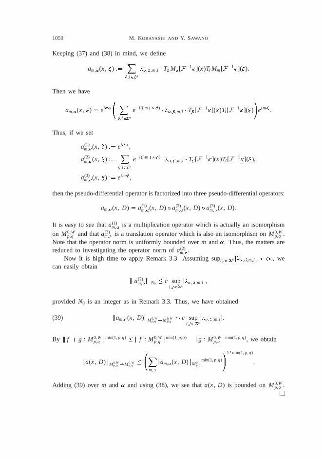
Keeping (37) and (38) in mind, we define

am,�(x, � ) WD X�,l2Zn

��,�,m,l � T�M�[F�1�](x)Tl Mm[F�1�](� ).

Then we have

am,�(x, � ) D ei��x X�,l2Zn

e�i (l �mC��) � ��,�,m,l � T� [F�1�](x)Tl [F�1�](� )

!eim�� .

Thus, if we set

a(1)m,�(x, � ) WD ei��x,

a(2)m,�(x, � ) WD X

�,l2Zn

e�i (l �mC��) � ��,�,m,l � T� [F�1�](x)Tl [F�1�](� ),

a(3)m,�(x, � ) WD eim�� ,

then the pseudo-differential operator is factorized into three pseudo-differential operators:

am,�(x, D) D a(1)m,�(x, D) Æ a(2)

m,�(x, D) Æ a(3)m,�(x, D).

It is easy to see thata(1)m,� is a multiplication operator which is actually an isomorphism

on M0,Wp,q and thata(3)

m,� is a translation operator which is also an isomorphism onM0,Wp,q .

Note that the operator norm is uniformly bounded overm and�. Thus, the matters arereduced to investigating the operator norm ofa(2)

m,�.Now it is high time to apply Remark 3.3. Assuming supl ,�2Zn j��,�,m,l j < 1, we

can easily obtain

kja(2)m,�jkN0 � c sup

l ,�2Znj��,�,m,l j,

provided N0 is an integer as in Remark 3.3. Thus, we have obtained

(39) kam,�(x, D)kM0,Wp,q !M0,W

p,q� c sup

l ,�2Znj��,�,m,l j.

By k f C g W M0,Wp,q kmin(1,p,q) � k f W M0,W

p,q kmin(1,p,q) C kg W M0,Wp,q kmin(1,p,q), we obtain

ka(x, D)kM0,Wp,q !M0,W

p,q� X

m,�kam,�(x, D)kM0p,q

min(1,p,q)

!1=min(1,p,q)

.

Adding (39) overm and � and using (38), we see thata(x, D) is bounded onM0,Wp,q .


4. Dual space

We will apply our decomposition results to specify the dual space ofMsp,q D Ms,1

p,q.We remark that in [19] we have obtained some results even for 0< p, q <1 and sD0. Our approach here is taking full advantage of Theorem 1.3 to prove the following.Given a p 2 (0,1], we define p0 WD p=(p� 1) if p > 1 and p0 WD 1 if p � 1.

Theorem 4.1. Let 0< p, q <1 and s2 R.1. Let f 2 M�s

p0,q0 . Then the functional g2 S 7! h f , gi 2 C can be extended to acontinuous linear functional on Msp,q.2. Conversely any continuous linear functional on Ms

p,q can be realized with f2 M�sp0,q0 .

Proof. The proof of 1 is straightforward and we omit the detail. We shall prove2 only in the case when 0< p � 1 � q < 1, the rest being covered in [19] whensD 0. An argument similar to the one below works for the remaining case. Let� bea continuous functional onMs

p,q. Then we can define the continuous operatorR frommp,q to Ms

p,q as follows: Let

R(�)(x) WD Xm,l2Zn

�ml � hmi�sTl Mm[F�1�](x),

where � is a function appearing in Theorem 1.3. Set WD � Æ RW mp,q ! C. Then is a continuous functional onmp,q. As is well-known, any continuous functional onmp,q can be realized with a coupling, that is, (�) can be expressed as

(�) D Xm,l2Zn

�ml � �ml, � D f�mlgm,l2Zn with k� W m1,q0k � ck� Æ Rk�,where� D f�mlgm,l2Zn 2 m1,q0 and k � k� denotes the operator norm. Be reminded that� is a function satisfying (7) to define the normk f W Ms

p,qk. Setting

S(g) WD fhmisTm�(D)g(l )gl ,m2Zn , g 2 Msp,q,

we obtain a linear mappingSW Msp,q ! mp,q satisfying

kS(g) W mp,qk � ckg W Msp,qk, � D � Æ R Æ SD Æ S.

Thus, we have� (g) D (fhmisTm�(D)g(l )gl ,m2Zn) DPm,l2Znhmis�ml � Tm�(D)g(l ) for

all g 2 Msp,q. Now we set f WD (2�)�n=2 P

m,l2Znhmis�ml � Tl M�m[F�]. Then The-orem 1.3 gives us

f 2 M�s1,q0 , k f W M�s1,q0k � ck� W m1,q0k � ck� Æ Rk� � ck�k�.


A simple calculation yields

h f , gi D (2�)�n=2 Xm,l2Zn

hmis�ml � hTl M�m[F�], giD (2�)�n=2 X

m,l2Zn

hmis�ml � hF�1[Tm�](l � �), giD � (g)

for all g 2 S. Therefore, 2 is proved.

ACKNOWLEDGEMENT. In writing this paper, the second author is supported finan-cially by Research Fellowships of the Japan Society for the Promotion of Science forYoung Scientists. The authors are grateful to Dr. Simon. Truscott for checking our presen-tation in English. The authors express deep gratitude to Professor Kerlheinz Gröchenig,Professor Hans Georg Feichtinger, Professor Joachim Toft and Professor Akihiko Miyachifor their giving the authors important information on the modulation spaces. Finally theauthors are indebted to the anonymous referee who read our manuscript carefully and gaveus important comments.

References

[1] R. Balan, P.G. Casazza, C. Heil and Z. Landau:Density, overcompleteness, and localization offrames, II, Gabor systems, J. Fourier Anal. Appl.12 (2006), 309–344.

[2] Á. Bényi, K. Gröchenig, K. Okoudjou and L. Rogers:Unimodular Fourier multipliers for mod-ulation spaces, J. Funct. Anal.246 (2007), 366–384.

[3] B. Wang and C. Huang:Frequency-uniform decomposition method for the generalized BO, KdVand NLS equations, J. Differential Equations239 (2007), 213–250.

[4] A.-P. Calderón and R. Vaillancourt:On the boundedness of pseudo-differential operators, J.Math. Soc. Japan23 (1971), 374–378.

[5] M. Frazier and B. Jawerth:A discrete transform and decompositions of distribution spaces, J.Funct. Anal.93 (1990), 34–170.

[6] H.G. Feichtinger: Modulation spaces on locally compact abelian groups; in M. Krishna,R. Radha and S. Thangavelu (Eds.): Wavelets and Their Applications, Chennai, India, AlliedPublishers, New Delhi, 99–140, 2003, updated version of a technical report, University ofVienna, 1983.

[7] H.G. Feichtinger:Atomic characterizations of modulation spaces through Gabor-type represen-tations, Constructive Function Theory—86 Conference (Edmonton, AB, 1986), Rocky Moun-tain J. Math.19 (1989), 113–125.

[8] H.G. Feichtinger: Gewichtsfunktionen auf lokalkompakten Gruppen, Österreich. Akad. Wiss.Math.-Natur. Kl. Sitzungsber. II188 (1979), 451–471.

[9] H.G. Feichtinger and K. Gröchenig:Gabor wavelets and the Heisenberg group: Gabor expan-sions and short time Fourier transform from the group theoretical point of view; in Wavelets,Academic Press, Boston, MA, 359–397, 1992.

[10] H.G. Feichtinger and K. Gröchenig:Gabor frames and time-frequency analysis of distributions,J. Funct. Anal.146 (1997), 464–495.


[11] Y.V. Galperin and S. Samarah:Time-frequency analysis on modulation spaces Mp,qm , 0< p, q �1, Appl. Comput. Harmon. Anal.16 (2004), 1–18.

[12] K. Gröchenig: Foundations of Time-Frequency Analysis, Applied and Numerical HarmonicAnalysis, Birkhäuser Boston, Boston, MA, 2001.

[13] K. Gröchenig:Composition and spectral invariance of pseudodifferential operators on modula-tion spaces, J. Anal. Math.98 (2006), 65–82.

[14] K. Gröchenig: Time-frequency analysis of Sjöstrand’s class, Rev. Mat. Iberoam.22 (2006),703–724.

[15] K. Gröchenig: Weight functions in time-frequency analysis; in Pseudo-Differential Operators:Partial Differential Equations and Time-Frequency Analysis, Fields Inst. Commun.52, Amer.Math. Soc., Providence, RI, 343–366, 2007.

[16] K. Gröchenig and C. Heil:Modulation spaces and pseudodifferential operators, Integral Equa-tions Operator Theory34 (1999), 439–457.

[17] K. Gröchenig and Z. Rzeszotnik:Banach algebras of pseudodifferential operators and theiralmost diagonalization, Ann. Inst. Fourier (Grenoble)58 (2008), 2279–2314.

[18] M. Kobayashi: Modulation spaces Mp,q for 0 < p, q � 1, J. Funct. Spaces Appl.4 (2006),329–341.

[19] M. Kobayashi:Dual of modulation spaces, J. Funct. Spaces Appl.5 (2007), 1–8.[20] B. Muckenhoupt:Weighted norm inequalities for the Hardy maximal function, Trans. Amer.

Math. Soc.165 (1972), 207–226.[21] B. Muckenhoupt: The equivalence of two conditions for weight functions, Studia Math.49

(1973/74), 101–106.[22] J. Sjöstrand:An algebra of pseudodifferential operators, Math. Res. Lett.1 (1994), 185–192.[23] M. Sugimoto and N. Tomita:A counterexample for boundedness of pseudo-differential opera-

tors on modulation spaces, Proc. Amer. Math. Soc.136 (2008), 1681–1690.[24] M. Sugimoto and N. Tomita:Boundedness properties of pseudo-differential and Calderón–

Zygmund operators on modulation spaces, J. Fourier Anal. Appl.14 (2008), 124–143.[25] K. Tachizawa:The boundedness of pseudodifferential operators on modulation spaces, Math.

Nachr.168 (1994), 263–277.[26] H. Triebel: Modulation spaces on the Euclidean n-space, Z. Anal. Anwendungen2 (1983),

443–457.[27] H. Triebel: Theory of Function Spaces, Birkhäuser, Basel, 1983.[28] H. Triebel: Theory of Function Spaces, II, Birkhäuser,Basel, 1992.

Masaharu KobayashiDepartment of MathematicsTokyo University of Science1-3 Kagurazaka, Shinjuku-ku, Tokyo 162–8601Japane-mail: [email protected]

Yoshihiro SawanoDepartment of Mathematics Kyoto UniversityKyoto 606-8502Japane-mail: [email protected]

molecular decomposition of the modulation spaces

Documents