On decomposable random graphs and link prediction

models

Mohamad Elmasri

Department of Mathematics and Statistics

McGill University, Montreal

August 2017

A thesis submitted to McGill University in partial fulllment of the

requirements for the degree of Doctor of Philosophy

c⃝ Mohamad Elmasri 2017

i

Abstract

In combinatorial graph theory, decomposable graphs are such type of graphs that are guar-

anteed to be decomposable into conditionally independent components, known as maximal

cliques. In statistics, decomposable graphs are widely used in the eld of graphical models

or Bayesian model determination, where the dependency structure among high dimensional

data or model parameters is unknown. Decomposable graphs are hence used as functional

priors over large covariance matrices or as priors over hierarchies of model parameters. One

such example is the Gaussian graphical model (Lauritzen, 1996; Whittaker, 2009), which has

seen success in a variety of applications. Beyond this framework, decomposable graphs are

seldom used in statistical applications.

Random graphs, on the other hand, have recently seen much research interest, where the

focus is on developing methodologies for models on relational data in the form of random

binary matrices. A principle component of such models is to assume a network framework

by mapping the relations to edges of the network, and data sources to nodes. The likelihood

of an edge is assumed to be driven by anity parameters of the associated nodes.

The rst part of this work attempts to propose a framework for modelling random de-

composable graphs, using similar tools as in random graphs. Rather than modelling edges

between nodes, the framework models the bipartite links between the graph nodes and latent

community nodes, through node anity parameters. The latent communities are assumed

to represent the maximal cliques in decomposable graphs. Under the proposed framework,

simple Markov update rules are given with explicit lower bounds for its mixing time (time

ii

until convergence). Under a set of conditions, an exact expression for the expected number

of maximal cliques per node is given.

The second part of this work illustrates a new application of decomposable graphs that is

motivated by the proposed framework. Combinatorially, there is a unique set of subgraphs of

any maximal clique. Treating maximal cliques as latent communities allows the treatment of

subgraphs of maximal cliques as sub-clusters within each community. The proposed frame-

work is extended to incorporate a sub-clustering component, which enables the modelling

of decomposable graphs and simultaneous modelling of the sub-clustering dynamics forming

within each larger community.

The nal part of this work deals with the topic of link prediction in networks with

presence-only data, where absence is only an indication of missing information and not a

prohibited link. The work is motivated by a particular example of identifying undocumented

or potential interactions among species from the set of available documented interactions,

in an aim to help guide the sampling of ecological networks by identifying the most likely

undocumented interactions. The problem is framed in bipartite graph structure, where

edges represent interactions between pairs of species. The work rst constructs a Bayesian

latent score model, which ranks observed edges from the most probable down to the least

certain. To improve scoring eciency, and thus link prediction, the work incorporates a

Markov random eld component informed by phylogenetic relationships among species. The

model is validated using two host-parasite networks constructed from published databases,

the Global Mammal Parasite Database and the Enhanced Infectious Diseases database, each

with thousands of pairwise interactions. Finally, the model is extended by integrating a

correction mechanism for missing interactions in the observed data, which proves valuable

in reducing uncertainty in unobserved interactions.

iii

Résumé

En théorie des graphes combinatoire, les graphes décomposables sont un type de graphe

dont il est garanti qu'ils sont décomposables en composantes conditionnellement indépen-

dantes, appelées cliques maximum. En statistiques, les graphes décomposables sont com-

munément utilisés dans le champ des modèles graphiques ou dans la détermination de mod-

èles Bayésiens, pour lesquels la structure de dépendence entre variables à haute dimensional-

ité ou des paramètres du modèle est inconnue. Les graphes décomposables sont ainsi utilisés

comme précédents fonctionnels par rapport aux matrices à large covariance ou en tant que

précédents par rapport aux hierarchies des paramètres du modèle. Un exemple de cette

utilisation est celle du modèle graphique Gaussien Lauritzen (1996); Whittaker (2009) qui a

été appliqué avec succès dans un grand nombre de cas.

Les graphes aléatoires ont généré beaucoup d'intérêt, en particulier, sur les données

relationnelles en de matrices aléatoires binaires. Une composante principale de ces modèles

est la dénition d'un cadre de réseau en associant les relations aux liens du réseau et les

sources de données aux noeuds.

La première partie de ce travail propose un cadre de modèlisation pour les graphes décom-

posables aléatoires et utilise des outils similaires à ceux utilisés pour les graphes aléatoires.

Plutôt que de modèliser les liens entre les noeuds, le cadre modèlise les associations bipartites

entre les noeuds du graphe et les noeuds des communautés latentes, à l'aide des paramètres

d'anité entre les noeuds. L'hypothèse émise étant que les communautés latentes représen-

tent les cliques maximum des graphes décomposables. Au sein de ce cadre proposé, les règles

iv

simples de mise à jour de Markov se voient attribuées une limite basse explicite pour leur

temps mélangé (temps sous convergence).

La seconde partie de ce travail illustre une nouvelle application des graphes décompos-

ables s'appuyant sur le cadre proposé. Combinatoirement, il existe un ensemble unique de

sous-graphes pour toute clique maximum. En traitant chaque clique maximum en tant que

communauté latente il est possible de traiter les sous-graphes des cliques maximum en tant

que sous-group au sein de chaque communauté. Le cadre proposé est étendu pour incorporer

une composante de sous-groupement, ce qui autorise la modélisation des graphes décompos-

ables et simultanément la modélisation de dynamiques de sous-groupement qui se forment

au sein de chaque communauté plus large.

La dernière partie de ce travail traite du sujet des prédictions de lien pour les réseaux

avec des données présence uniquement, où l'abscence est seulement une indication de don-

nées manquantes et non d'un lien interdit. Ce travail s'appuie sur un exemple specique,

celui de l'identication d'interactions non-documentées ou potentielles au sein d'espèces

appartennant à l'ensemble des interactions documentées. L'objectif est d'aider à guider

l'échantillonnage de réseaux écologiques en identiant les relation non-documentées les plus

vraisemblables. Le problème est cadré en structure bipartite de graphe où les liens représen-

tent les interactions entre paires d'espèces. Le travail développe tout d'abord un modèle

de score latent Bayésien qui ordonne les liens observés du plus probable au moins certain.

Pour améliorer l'ecience du score et partant la prédiction des liens, le travail incorpore

un composant de champ aléatoire de Markov utilisant lesretations phylogéniques entre es-

pèces. Le modèle est validé en utilisant deux réseaux hôte/parasite construits à partir de

deux bases de données publiées; la base globale mammifère parasiteet la base de données

améliorée des maladie infectieuses, chacune contenant des milliers de paires d'interactions.

Finalement, le modèle est étendu en intégrant un méchanisme de correction pour les inter-

actions manquantes dans les données observées, qui s'avère ecace à diminuer l'incertitude

dans les interactions inobservées.

v

Acknowledgments

First and foremost, I am sincerely grateful to my supervisor, Professor David A. Stephens.

Since my early days in the Doctoral programme, he encouraged me to follow my own research

path, gave me ample room to learn and grow academically and professionally, was generous

with nancial support, and always provided valuable suggestions.

I am also grateful to the faculty of the Department of Mathematics and Statistics for their

excellent graduate courses that were essential to my learning. Thanks to the administrative

and IT sta of the department for their help through many applications and other paper

work, and thanks to the cleaning team that kept our oces tidy and boards clean.

I am especially grateful to Professor Russell Steele, for his unyielding optimism and

encouragement, and for being instrumental in shaping the student-run Stat and Biology

Exchange group (S-Bex). A large part of this work has been motivated by the problems and

ideas discussed in this inter-disciplinary group. Thanks to Amanda Winegardner and Zoa

Taranu for organizing S-Bex and for making it such an enjoyable experience. I would also

like to thank Maxwell Farrell, an S-Bex member, with whom I spent much time discussing

ideas and collaborating on research work.

Thanks to all the friends that helped me during those years: Patrick Montjourides, Oscar

Xacur, Ivo Pendev, Jeno Grebennikov, Hassein Asmar, and many others, I can not stress

how thankful I am. I am very grateful to Friedrich Huebler from the UNESCO Institute for

Statistics, for his professional mentorship and support.

I am indebted to my family in Montreal, for providing a second home and for all the

vi

delicious food and good times. Importantly, I'd like to express my never-ending gratitude

for a long list of things to my parents Maha and Ahmed and my siblings, Fatima, Ebrahim,

Maryam and Noor.

In no words I can describe how grateful I am to my wife Sheena Bell, who stood by my

side all along this journey. Without you, this simply could not have been accomplished.

I would like to thank the Lorne Trottier Science Accelerator Fellowships, Fonds de

recherche du Québec - Nature et technologies (FRQNT), and the Department Graduate

Awards, for their generous nancial support. I also like to thank the examiners and defence

committee for their comments and valuable feedback, and thanks to everyone that helped in

editing this document.

vii

Contents

Abstract i

Résumé iii

Acknowledgments v

List of Figures xvi

List of Tables xviii

1 Introduction 1

1.1 Thesis contribution . . . . . . . . . . . . . . . . . . . . . . . . . . . . . . . . 5

1.2 Thesis outline . . . . . . . . . . . . . . . . . . . . . . . . . . . . . . . . . . . 7

2 Background 8

2.1 Poisson process . . . . . . . . . . . . . . . . . . . . . . . . . . . . . . . . . . 8

2.1.1 Key properties of Poisson processes . . . . . . . . . . . . . . . . . . . 11

2.1.2 The Cox process . . . . . . . . . . . . . . . . . . . . . . . . . . . . . 13

2.2 Bayesian models for exchangeable graphs . . . . . . . . . . . . . . . . . . . . 14

2.2.1 The de Finetti representation of sequences . . . . . . . . . . . . . . . 16

2.2.2 The Aldous-Hoover representation theorem for random graphs . . . . 18

2.2.3 Exchangeable graphs as exchangeable 2-arrays . . . . . . . . . . . . . 20

2.2.4 The Kallenberg representation theorem for random graphs . . . . . . 22

Contents viii

2.2.5 Exchangeable graphs as exchangeable measures on R2+ . . . . . . . . 25

2.3 Completely random measures . . . . . . . . . . . . . . . . . . . . . . . . . . 27

2.3.1 Sampling CRM from unit rate Poisson processes . . . . . . . . . . . . 31

2.3.1.1 Homogeneous CRMs . . . . . . . . . . . . . . . . . . . . . . 33

2.3.1.2 Inhomogeneous CRMs . . . . . . . . . . . . . . . . . . . . . 33

3 Decomposable random graphs 35

3.1 Introduction . . . . . . . . . . . . . . . . . . . . . . . . . . . . . . . . . . . . 35

3.2 Preliminaries . . . . . . . . . . . . . . . . . . . . . . . . . . . . . . . . . . . 37

3.2.1 Decomposable graphs . . . . . . . . . . . . . . . . . . . . . . . . . . . 37

3.2.2 Models for decomposable graphs . . . . . . . . . . . . . . . . . . . . . 40

3.3 Decomposable random graphs by conditioning on junction trees . . . . . . . 42

3.3.1 Decomposable graph as point processes. . . . . . . . . . . . . . . . . 47

3.3.2 Finite graphs forming from domain restrictions . . . . . . . . . . . . 50

3.3.2.1 Augmentation by an identity matrix . . . . . . . . . . . . . 53

3.3.2.2 Likelihood factorization with respect to Z . . . . . . . . . . 57

3.4 Exact sampling conditional on a junction tree . . . . . . . . . . . . . . . . . 59

3.4.1 Sequential sampling with nite steps . . . . . . . . . . . . . . . . . . 60

3.4.2 Sampling using a Markov stopped process . . . . . . . . . . . . . . . 61

3.4.2.1 Mixing time of the stopped process . . . . . . . . . . . . . . 62

3.5 Edge updates on a junction tree . . . . . . . . . . . . . . . . . . . . . . . . . 65

3.6 Examples . . . . . . . . . . . . . . . . . . . . . . . . . . . . . . . . . . . . . 68

3.6.0.2 On the joint distribution of a realization . . . . . . . . . . . 69

3.6.1 The multiplicative model . . . . . . . . . . . . . . . . . . . . . . . . . 71

3.6.1.1 Posterior distribution for the special case of a single marginal 72

3.6.1.2 Inference by Gibbs sampling . . . . . . . . . . . . . . . . . . 76

3.6.2 The log transformed multiplicative model . . . . . . . . . . . . . . . . 76

3.6.2.1 Posterior distribution for the two marginals . . . . . . . . . 77

Contents ix

3.7 Model properties: Expected number of cliques per node . . . . . . . . . . . . 79

3.8 Discussion . . . . . . . . . . . . . . . . . . . . . . . . . . . . . . . . . . . . . 86

4 Sub-clustering in decomposable graphs and size-varying junction trees 88

4.1 Introduction . . . . . . . . . . . . . . . . . . . . . . . . . . . . . . . . . . . . 88

4.2 Subgraphs of cliques as sub-clusters . . . . . . . . . . . . . . . . . . . . . . . 89

4.3 Permissible moves in the bipartite relation . . . . . . . . . . . . . . . . . . . 90

4.3.1 Disconnecting single-clique nodes . . . . . . . . . . . . . . . . . . . . 92

4.3.2 Disconnecting multi-clique nodes . . . . . . . . . . . . . . . . . . . . 94

4.3.3 Connecting nodes . . . . . . . . . . . . . . . . . . . . . . . . . . . . . 99

4.4 Promoting a sub-clique to be maximal . . . . . . . . . . . . . . . . . . . . . 101

4.5 Markov updates under size-varying junction trees . . . . . . . . . . . . . . . 103

4.6 Discussion . . . . . . . . . . . . . . . . . . . . . . . . . . . . . . . . . . . . . 104

5 A Bayesian model for link prediction in ecological networks 107

5.1 Introduction . . . . . . . . . . . . . . . . . . . . . . . . . . . . . . . . . . . . 108

5.2 Bayesian hierarchical model for prediction of ecological interactions . . . . . 109

5.2.1 Network-based latent score model . . . . . . . . . . . . . . . . . . . . 109

5.2.2 Prior and Posterior distribution of choice parameters . . . . . . . . . 113

5.2.3 Markov Chain Monte Carlo algorithm . . . . . . . . . . . . . . . . . . 115

5.3 Uncertainty in unobserved interactions . . . . . . . . . . . . . . . . . . . . . 116

5.3.1 Markov Chain Monte Carlo algorithm . . . . . . . . . . . . . . . . . . 118

5.4 A case study with host-parasite networks . . . . . . . . . . . . . . . . . . . . 119

5.4.1 Data . . . . . . . . . . . . . . . . . . . . . . . . . . . . . . . . . . . . 119

5.4.2 Parameter estimation . . . . . . . . . . . . . . . . . . . . . . . . . . . 121

5.4.3 Prediction comparison by cross-validation . . . . . . . . . . . . . . . 122

5.4.4 Uncertainty in unobserved interactions . . . . . . . . . . . . . . . . . 126

5.5 Discussion . . . . . . . . . . . . . . . . . . . . . . . . . . . . . . . . . . . . . 130

Contents x

Appendices 133

A Latent formulation and sampling 134

A.1 Existence of the joint distribution . . . . . . . . . . . . . . . . . . . . . . . . 138

A.1.1 Parametrization using an exponential distribution . . . . . . . . . . . 138

A.2 Latent score sampling with uncertainty . . . . . . . . . . . . . . . . . . . . . 139

B Details on the MCMC algorithm 141

C Additional results 145

C.1 Posterior distributions . . . . . . . . . . . . . . . . . . . . . . . . . . . . . . 145

C.2 Representative trace plots and diagnostics . . . . . . . . . . . . . . . . . . . 146

C.3 Parameter numerical results . . . . . . . . . . . . . . . . . . . . . . . . . . . 148

C.4 Uncertainty - histograms . . . . . . . . . . . . . . . . . . . . . . . . . . . . . 149

C.5 Interaction matrices for subsets - Carnivora and Rodentia . . . . . . . . . . . 150

C.6 ROC with and without g for full GMPD and EID2 databases . . . . . . . . . 151

C.7 Percentage of recovered pairwise interactions . . . . . . . . . . . . . . . . . . 154

C.8 Posterior degree distribution . . . . . . . . . . . . . . . . . . . . . . . . . . . 155

C.9 Hyperparameters and eective size . . . . . . . . . . . . . . . . . . . . . . . 156

6 Conclusion and future research 158

6.1 Future research . . . . . . . . . . . . . . . . . . . . . . . . . . . . . . . . . . 160

xi

List of Figures

2.1 An example of a simple graph generated under the Kallenberg representation.

The top left corner shows a generated Poisson point process (θi, ϑi) with

restrictions on the location (x-axis) and weight (y-axis) domains shown in dot-

ted grey lines, points outside the restricted cube are shown with grey circles.

Using the point process and the cohesion function W shown by the heat map

in the top right corner, we generate a random simple graph as shown in the

bottom left corner, where only nodes with active edges are shown; in black

circles are nodes within the restricted cube, in grey are nodes outside the re-

stricted cube though with active edges. The graph is shown in the bottom

right corner with the same colour coding. . . . . . . . . . . . . . . . . . . . . 28

3.1 An undirected decomposable graphs of 4 cliques of size 3; ABC, BEF, BCE,CDE. 38

3.2 A decomposable graph and its bipartite graph linking junction trees of cliques

and perfect orderings. . . . . . . . . . . . . . . . . . . . . . . . . . . . . . . . 40

3.3 An example of arbitrary adding an edge between nodes in a decomposable

graph: on the left is the original graph, in the middle, node E joins clique

AD causing a change in the junction tree while preserving decomposability,

on the right, node F joins clique ABC, abolishing decomposability by forming

the circle ADEF with no inner chord. . . . . . . . . . . . . . . . . . . . . . . 44

List of Figures xii

3.4 A realization of a decomposable graph in 3.4d from the point process in 3.4a

and the tree 3.4b. The grey area in 3.4a is the edge-greedy partition (r, ro],

where only one extra node (in blue) was needed to guarantee all active cliques

are maximal, since Zr′,r(θ′3∩.) is a subset of Zr′,r(θ′6∩.) and Zr′,r(θ′7∩.).

3.4c is the biadjacency matrix of active (clique-)nodes representing the graph. 52

3.5 Relaxation of (3.13) by removing the empty rows in the realization of Figure

3.4c and augmenting the results with an identity matrix. . . . . . . . . . . . 54

3.6 A realization of a 5-node junction tree from (3.21), on the left is the original

directed weighted tree where Wk = W (ϑ′k, ϑi) for a random ϑi, on the right is

the undirected tree by expectation where W∗ = E(W ). . . . . . . . . . . . . 65

3.7 Moving along the bipartite graph of Figure 3.2, from junction tree T1 to T2,

through severing and reconnecting the edge C2, C3 (dotted lines) to C2, C1. 66

3.8 Density of W (x, y) = exp(−(x+ y)). . . . . . . . . . . . . . . . . . . . . . . 72

3.9 Dierent size realizations from W (x, y) = exp(−(λ1x + λ2y)); the 10-node

tree on the top left is sampled according to (3.21) with a (c′ = 1, r′ = 10)-

truncation. The top and middle panels are the decomposable graphs resulting

from dierent size realization settings, the middle panel illustrates the eect of

varying λ2 for the same parameter set (θi, ϑi) generated from a (c = 2, r =

50)-truncation, the corresponding adjacency matrices are in the bottom panel. 73

3.10 Junction tree, decomposable graph, and posterior MCMC trace plots for three

randomly selected nodes, where fiiid∼ Beta(α, 1), for the single marginal dis-

tribution of W (x, y) = f(y). . . . . . . . . . . . . . . . . . . . . . . . . . . . 75

3.11 Junction tree, decomposable graph, and the posterior MCMC trace plot of

ϑi = ϑ = 0.3, for the case W (ϑ′k, ϑi) = ϑ. . . . . . . . . . . . . . . . . . . . . 75

3.12 A binary 3-regular tree, with 10-nodes including the root node ϑ′0 and over

two levels (L = 2). . . . . . . . . . . . . . . . . . . . . . . . . . . . . . . . . 81

List of Figures xiii

4.1 A 4-node clique (left) and all its unique subgraphs, including single-node

cliques, for a total of 15 subgraphs. . . . . . . . . . . . . . . . . . . . . . . . 89

4.2 An example of a biadjacency matrix (left), with 5 maximal cliques, stared and

in red, and 10 sub-cliques. The corresponding junction tree (top right) has all

sub-cliques and their ascendants circulated and connected with dashed lines,

with maximal cliques in red solid lines. The decomposable graph (bottom

right) summarizes the biadjacency matrix. . . . . . . . . . . . . . . . . . . . 91

4.3 Examples of disconnecting single-clique nodes of the graph in Figure 4.2. The

top panel shows the case when disconnecting node A from clique ABCD (top

left), where BCD is still maximal, and the previous sub-clique AB is now

maximal, adding another clique-node to the junction tree joined at BCD (top

right), while discarding all other sub-cliques that contain A with nodes C or

D, as AC. The middle row shows the case when disconnecting node G from

FGH (middle left), where FH is still maximal, while the previous sub-clique

GH is now maximal adding an extra clique-node to the junction tree (middle

right) connected to FH. The bottom panel shows the case when a maximal

clique becomes sub-maximal, by disconnecting the node E from CEF (bottom

left), where CF is now a sub-clique of CEF (shown dashed and in blue),

thus removing the corresponding clique-node from the junction tree (bottom

right), while connecting all previous CEF edges to CDF. The new maximal

clique-node EF adds an edge to the tree with CDF. . . . . . . . . . . . . . . 95

4.4 An example: disconnecting a multi-clique node D from the maximal clique

ABCD in Z and G, where the resulting graph G ′ is decomposable albeit Z′ is

not its representative bipartite matrix; missing the maximal clique BCD in G ′. 98

List of Figures xiv

4.5 Examples of disconnecting multi-clique nodes of the example in Figure 4.2.

The graph in the top panel (top left) shows the example of disconnecting C

from ABCD, cases (i.c) and (ii.a) of Proposition 6, where the separator CD

belongs to the sub-clique ACD, making it maximal. The junction tree (top

right) is rewired accordingly, and no sub-clique is discarded. The graph in

the bottom panel (bottom left) illustrates the case of disconnecting H from

FGH to form FG, while discarding the sub-clique GH, as in (i.a) and (ii.a)

of Proposition 6, since FG∩HI is empty, the junction tree (bottom right) is

rewired accordingly. . . . . . . . . . . . . . . . . . . . . . . . . . . . . . . . . 99

4.6 An example of connecting a node to a sub-clique in an adjacent maximal

clique. Node H connects to the sub-clique EF (left) from the example in

Figure 4.2, by (iii) of Corollary 5 this forms the new maximal clique EFH

connecting maximal cliques CEF and FGH. . . . . . . . . . . . . . . . . . . 102

5.1 Left ordered interaction matrix Z of GMPD (left) and EID2 (right) databases. 120

5.2 Degree distribution of hosts (red crosses) and parasites (blue stars) on log-

scale, for the GMPD (left) and EID2 (right) databases. . . . . . . . . . . . . 121

5.3 ROC comparison of the latent score (LS) network model with three varia-

tions and the regular NN algorithm. The proposed LS full model in black,

the anity-only variation in cyan, phylogeny-only variation in grey, and the

weighted-by-counts version in green. The regular NN algorithm in brown. All

ROC curves are based on an average of 10-fold cross-validations. . . . . . . . 124

5.4 Posterior associations matrix comparison: for the GMPD (top panel) and

EID2 (bottom panel), between the anity-only (left), phylogeny-only (mid-

dle) and full model (right). . . . . . . . . . . . . . . . . . . . . . . . . . . . . 126

5.5 Comparison of ROC curves for the model with g (black) and without g (grey),

for GMPD-Carnivora on the left and the EID2-Rodentia on the right. . . . . 128

List of Figures xv

C.1 Boxplots of posterior estimates for the host and parasite parameters with the

80 highest medians, and the posterior distributions of the scale parameter,

dashed horizontal lines are the mean posterior and 95% credible intervals, for

the GMPD (top panel) and EID2 (bottom panel). . . . . . . . . . . . . . . . 146

C.2 Trace plots for the GMPD and EID2: host (top) and parasite (middle) of

highest median posterior, and the similarity matrix scaling parameter (bottom).147

C.3 ACF plots and eective sample sizes for the GMPD and EID2: host (top)

and parasite (middle) of highest median posterior, and the similarity matrix

scaling parameter (bottom). . . . . . . . . . . . . . . . . . . . . . . . . . . . 147

C.4 Posterior histogram for g for the GMPD (left) and EID2 (right) databases. . 149

C.5 Comparison in posterior log-probability between observed and unobserved in-

teractions, for the model without g (left) and with g (right), for the GMPD-

Carnivora database. . . . . . . . . . . . . . . . . . . . . . . . . . . . . . . . . 150

C.6 Association matrices of the whole GMPD-Carnivora subset: Observed (left),

posterior for the model without g (middle), posterior for the model with g

(right). . . . . . . . . . . . . . . . . . . . . . . . . . . . . . . . . . . . . . . . 150

C.7 Association matrices of the whole EID2-Rodentia subset: Observed (left),

posterior for the model without g (middle), posterior for the model with g

(right). . . . . . . . . . . . . . . . . . . . . . . . . . . . . . . . . . . . . . . . 151

C.8 Comparison of ROC curves for the full dataset, for the models with(out) g. . 151

C.9 Posterior association matrices for the full datasets. . . . . . . . . . . . . . . . 152

C.10 Number of pairwise recovered interactions from the original data. . . . . . . 154

C.11 Comparison of degree distribution on log-scale, for the full model (without

accounting for uncertainty) and the model with g, GMPD dataset. . . . . . . 155

C.12 Comparison of degree distribution on log-scale, for the full model (without

accounting for uncertainty) and the model with g, EID2 dataset. . . . . . . . 156

List of Figures xvi

C.13 Trace plots of convergence of three chains started at dierent values for the

expected value of the hyperparameter for the GMPD dataset . . . . . . . . . 157

xvii

List of Tables

2.1 Summary of some known models admitting the graphon representation. . . . 22

3.1 Possible prefect ordering of cliques of Figure 3.1 . . . . . . . . . . . . . . . . 39

3.2 A summary table of the number of clique-nodes at distance k from clique-

nodes at level ℓ ≤ L for a d-regular tree with L levels, where ⌊x⌋ is the oor

operator and d = (d− 1). . . . . . . . . . . . . . . . . . . . . . . . . . . . . . 83

4.1 Multi-clique nodes of example in Figure 4.2, their disconnect from maximal

cliques, separator sets and possible sub-cliques to become maximal. . . . . . 98

5.1 Area under the curve and prediction values for tested models . . . . . . . . . 125

5.2 Two-sided Wilcoxon signed rank test to compare model AUCs . . . . . . . . 125

5.3 AUC comparison between models with g and without g on the GMPD and

EID2 databases and clade subsets . . . . . . . . . . . . . . . . . . . . . . . . 129

5.4 Percentage of observed interactions correctly predicted in the held-out portion

of the validation set (in parentheses) and in the full data, for the GMPD and

EID2 databases . . . . . . . . . . . . . . . . . . . . . . . . . . . . . . . . . . 130

C.1 Posterior means, Monte Carlo standard errors and credible intervals for the

highest anity parameters and the scale parameter. . . . . . . . . . . . . . . 148

C.2 AUC comparison between models with g and without g, on the GMPD databases

and clade subsets, with dierent variations of the model . . . . . . . . . . . . 152

List of Tables xviii

C.3 Percentage of observed interactions correctly predicted in the held-out portion

of the validation set (in parentheses) and in the full data, for the GMPD database152

C.4 AUC comparison between models with g and without g, on the EID2 databases

and clade subsets, with dierent variations of the model . . . . . . . . . . . . 153

C.5 Percentage of observed interactions correctly predicted in the held-out portion

of the validation set (in parentheses) and in the full data, for the EID2 database153

1

Chapter 1

Introduction

With technology advancing, data gathering capacity is consistently improving and new forms

of data are emerging. Some forms adhere to the classical 1-dimensional sequential observa-

tions, which represent the randomness in the data sources. Others dier from the classical

type, in a sense that they represent relationships between two or more data sources or objects.

Structured relational data is one type of such new forms of data which gained prominence in

graph and network based technologies, where pairwise relationships between network nodes

are of interest. For example, structured relational data proved essential in biology as a tool

to summarize complex multi-way relationships amongst organisms, and to predict unknown

interactions. Applications of such data extends to many other elds.

The statistical community, on the other hand, is consistently developing empirical models

to analyze new emerging forms of data. For the case of relational data, some of the popular

recently developed models are the blockmodel (Wang and Wong, 1987), latent distance model

(Ho et al., 2002), and the innite relational model (Kemp et al., 2006), and their variations.

Under certain assumptions, some models provide strong theoretical and asymptotic results,

nonetheless, most are intrinsically misspecied for many real-world applications, especially

for large networks, where a sparseness property is essential (Newman, 2010). Sparseness is

generally dened as the proportion of relations (edges) to the number objects (nodes), if edges

1 Introduction 2

grow linearly with respect to nodes then the dataset is described as sparse, otherwise as dense.

The lack of the sparseness property in most initial models is due to the theoretical foundation

those models are built upon, which regards relational data as random observations of random

arrays or matrices. Progress has been achieved recently in this domain by adapting a dierent

theoretical foundation which builds on continuous-time stochastic processes. In this sense, a

real world relational dataset is seen as a sample from an unknown continuous-time process

(Borgs et al., 2015, 2016, 2014a,b; Caron and Fox, 2014; Janson, 2016; Veitch and Roy,

2015). The new framework provides many rich results associated with stochastic processes,

though challenges still exist in the area of nonparametric estimation of such multidimensional

processes.

Models for relational data were initially inuenced by the introduction of probabilistic

methods to graph theory, most notably the work of Erdös and Rényi (1959), which studied

asymptotic probability of graph connectivity. This introduction gave rise to a branch of

mathematics known as random graph theory, which includes most of the probabilistic models

for relational data. A larger branch of graph theory existed much earlier, dating back to 1736

to a paper written by Leonhard Euler on the Seven Bridges problem (Biggs et al., 1976).

Since then, research in graph theory mostly fell in the domain of discrete mathematics and

produced many rich results, such as the characterizations of dierent types of graphs and

their properties, which have also seen great applications in statistics outside the eld of

relational data modelling.

Decomposable (chordal) graphs are such a type of well studied objects in discrete math-

ematics that have seen wide applicability in statistics. A graph is said to be decomposable

if, and only if, any cycle of four or more nodes has an edge (chord) that does not belong

to the cycle. This property ensures that a given graph can be decomposable into multiple

independent subgraphs, known as maximal cliques. If one views graph nodes as random

variates and graph edges as pairwise variate relations, then the decomposability property

translates to conditional independence between subsets of variates, or what is known as the

1 Introduction 3

Markov property. Such analogy enabled decomposable graphs to be used as functional pri-

ors over large covariance matrices or as priors over hierarchies of model parameters, which

gave rise to a branch of statistics known as graphical models, that aims to infer conditional

dependency simultaneously while inferring model parameters. Other types of graphs have

also seen applications in the branch of graphical models, nonetheless, the explicit interpreta-

tion of conditional dependencies in decomposable graphs have earned them special attention

in statistics, primarily because they greatly simplify the observational data likelihood. For

example, the Gaussian graphical model has seen success in a variety of applications of such

dependency nature (Lauritzen, 1996; Whittaker, 2009). In fact, the earliest introductions of

decomposable graphs to statistics is in the eld of Bayesian model determination, by Dar-

roch et al. (1980) and Wermuth and Lauritzen (1983), as a generating class of decomposable

log-linear models on multidimensional contingency tables.

A few eorts in statistics exists that utilize decomposable graphs beyond graphical mod-

els, for example, the work of Tank et al. (2015) that applied decomposable graphs for struc-

tural learning of time series, and the work of Caron and Doucet (2009) to Bayesian nonpara-

metric models. The lack of a broader statistical applicability of decomposable graphs could

be attributed to two aspects, a combinatorial one and a statistical one. The combinatorial

issues include, for example, ecient methods for testing for decomposability in large graphs,

and nding the largest fully connected component, where the latter is still an open problem.

The statistical issues include ecient sampling methods, where only recently a uniform,

though intricate, sampling algorithm is proposed in Thomas and Green (2009), with a more

ecient local update scheme by Stingo and Marchetti (2015).

A main focus of this work is to extend the recent developments in modelling of relational

data to modelling of, what we term, decomposable random graphs. In this framework,

we propose a generative model of decomposable graphs, where a sample of the model is a

random size biadjacency matrix and with a deterministic mapping function a decomposable

graph is attained. Edges are generated sequentially through probabilities driven by node

1 Introduction 4

specic parameters. The sequential generation guarantees decomposability of the graph

at each step, and is a native process in such context for the Markovian interpretation of

decomposability. The model builds on the work of Thomas and Green (2009), and adapts

a bipartite representation of the graph, between nodes and the maximum fully connected

components; the maximal cliques. Such representation is later extended to allow for a new

application of decomposable graphs, where one is not only able to model the graph, but also

simultaneously model latent sub-clusters within maximal cliques. The clustering mechanism

of the model evades two limitations of most clustering algorithms, choosing the correct

number of clusters, and choosing a proper distance metric for clustering. Both limitations

are addressed through the generation process and the construction of the model.

In practice, hierarchical clustering is fundamental to many applications, in fact, it is

natural in many systems in the real world. For example, the evolutionary tree of organisms

in biology, as well as the categorization of documents into topics in literature. Thus, we

anticipate a wide range of applications to the proposed model.

Another area of focus in this work is on the topic of link prediction in networks with

presence-only data. Conventionally, the existence of an edge in a network is an indication of

dependence or interaction among the pair of nodes connected by the edge, in reverse, a pair

of nodes are conditionally independent if there is no edge connecting them. This seems to

be the belief of most network-based models of relational data. Yet, the absence of an edge

in certain types of relational data is only an indication of unknown information, where the

true edge could exist but is currently unobserved, or forbidden as in the case of conditional

independence.

One example of interest to this work, is the case of identifying undocumented or potential

interactions among species from the set of available documented interactions. In an aim

to guide the sampling of ecological networks by identifying the most likely undocumented

interactions, this work tackles this problem by proposing a network based Bayesian latent

score model, in which scores are assigned to observed edges, much like the conventional

1 Introduction 5

network based models. This work improves on that by incorporating a Markov random

eld component, in this case the phylogenetic information which also depends on observed

edges. By estimating the parameters of the model, the posterior distribution is then used

to predict undocumented interactions. Since it is hard to know the exact number of actual

true interactions from forbidden ones, a measure of uncertainty is built which attempts to

estimate the false negative rate on the data source. This rate is then used to gauge the

predicted number of potential interactions.

1.1 Thesis contribution

The following is a list summarizing the contributions of this thesis.

• The class of decomposable graphs are extensively applied in the context of graphical

models, primarily due to its explicit interpretation of conditional dependencies that

greatly simplify the observational data likelihood. Chapter 3 attempts to extend the

statistical use of decomposable graphs by proposing a dierent modelling framework.

In the classical settings, decomposable graphs are modelled via the adjacency matrix,

instead, the proposed framework models them via their biadjacency matrix which

represent the connection between the graph nodes and the conditionally independent

components of the graph, known as maximal cliques. The decomposable graph is

retrieved by a deterministic mapping function. The framework represents maximal

cliques as latent communities with their specic membership parameters, mimicking

that of the graph node parameters. The likelihood of a node becoming a part of a

latent community depends on both of their specic parameters.

• The proposed biadjacency representation of decomposable graph in Chapter 3 yields

simple Markov update rules, enabling a sort of parallelization in the Monte Carlo

Markov Chain methods. As a result, the convergence time is minimized. Section

3.4 illustrates results on mixing time (time until convergence) for the proposed mod-

1 Introduction 6

elling framework. As a consequence of decoupling the graph nodes from the maximal

cliques, it is possible to compute the expected number of cliques per node, which is the

contribution of Section 3.7. This expectation, though exact, requires a certain set of

assumptions relating to the dependency structure among the maximal cliques, known

as the junction tree of the graph. Therefore, it is characterized conditionally.

• Chapter 4 generalizes the framework of Chapter 3 to open the door for a new applica-

tion of decomposable graphs. This is done by extending the biadjacency representation

to allow for interactions between graph nodes and subgraphs of maximal cliques. Sub-

graphs of maximal cliques can naturally be seen as sub-clusters within each maximal

clique. In fact, combinatorially, a maximal clique of N nodes has 2N − 1 unique clique

sub-graphs, including single nodes. The ability of the biadjacency representation to

account for such sub-clusters adds to its richness. Rather than solely modelling decom-

posable graphs, as in the classical settings, it is now possible to model the decomposable

graph and at the same time the latent dynamics forming within each maximal clique.

There are a few ways to address the dynamics of interactions between maximal cliques

and sub-clusters. Section 4.3 lists a series of propositions and corollaries illustrating

possible connect and disconnect moves in the biadjacency representation that guaran-

tee the decomposability of the graph. Section 4.5 summarizes all possible moves in

simpler Markov update steps.

• Most ecological networks, while highly critical to the functioning of ecosystems, are

only partially observed and fully characterizing them requires substantial sampling ef-

fort that is not feasible in most situations (Jordano, 2015). Many ecological networks

are often based on presence-only data, where an unobserved interaction may be either

present or absent. Chapter 5 introduces a latent score model for link prediction in eco-

logical networks, motivated by the class of Auto-models of Besag (1974). The proposed

model is a combination of two separate models: (i) an anity based exchangeable ran-

1 Introduction 7

dom networks model; (ii) a Markov random eld network model that is informed by

phylogeny. To account for uncertainty in unobserved interactions, inuenced by the

work of Jiang et al. (2011), Section 5.3 incorporates a measure of the proportion of

missing links in the observed data, which strengthens the posterior predictive accuracy

of the model. Section 5.4.3 compares the predictive performance of the proposed model

and three of its variates to a nearest-neighbour algorithm. The model is validated using

two host-parasite networks constructed from published databases, the Global Mammal

Parasite Database and the Enhanced Infectious Diseases database.

1.2 Thesis outline

This work is organized as follows, Chapter 2 is a literature review of specic topics that

relate to dierent parts of this work, where preliminary notations are also introduced. One

of the main results discussed in this chapter is the newly developed framework of random

graphs that builds on continuous-time stochastic processes, and its contrast to the initially

used framework of random arrays and matrices. Chapter 3 is one of the main contributions

of this work which proposes a model for decomposable random graphs. The preliminary

notation and background on decomposable graphs is also introduced in this chapter. Chap-

ter 4 is another contribution related to decomposable graphs, where the new application of

sub-clustering is introduced with a series of propositions addressing possible update moves.

Chapter 5 is the nal contribution of this work, which deals with link prediction in bipar-

tite networks with presence-only data. This chapter was initially submitted for publication

in a peer-reviewed journal, and thus formatted with appendices containing details on com-

putational aspects and additional convergence results relating to simulations and real data

examples. Finally, Chapter 6 summarizes the research contributions and discusses possible

future research directions.

8

Chapter 2

Background

2.1 Poisson process

The Poisson process, or the Poisson point process, is one of the most studied point processes

in many disciplines, due to its simplicity and favourable mathematical properties. It is

dened on a measurable space, most commonly the Euclidean space for practical reasons.

For example, the arrival times of customers, or the number of heads appearing in a sequence

of coin tossing. The naming is directly derived from its relation to the Poisson distribution,

where a random variable N is said to have a Poisson distribution with parameter µ if the

probability of an event occurring n ≥ 0 discrete times is

P(N = n) =µne−µ

n!. (2.1)

The parameter µ represents the expected number of occurrences, as

E[N ] =∞∑n=0

nP(N = n) = µ. (2.2)

Poisson processes are constructed by letting the random variable N of (2.1) to be a

count function over measurable subsets A over a space S. Such that, N(A) is the count

2 Background 9

of event occurrences in A, which is also distributed as a Poisson random variable with

parameter function µ(A). More formally, following the language of Billingsley (2008), dene

the probability triple (S,F ,P), where S is the elementary set of events, F is the σ-algebra

of subsets ("events") in S and P : S ↦→ [0, 1] is a probability measure on measurable subsets

in S.

Denition 1. A Poisson process, dened on a probability space (S,F ,P), is a point process

Π of countable sets of points in S. Such that, if A is a measurable subset of S, then the

number of points of Π in A is a well dened random variable measured as

N(A) = #Π ∩ A, (2.3)

and satisfy the following properties:

(i) for any disjoint countable subsets A1, A2, · · · ⊂ S the random variables N(A1), N(A2), . . .

are independent;

(ii) and for each i ∈ N, N(Ai) is a Poisson random variable with mean function 0 ≤

µ(Ai) ≤ ∞;

Note that for non-nite µ(A), Π ∩ A is countably innite with probability 1, and nite

with probability 1 if µ(A) is nite.

Remark. If S = Rd, a d-dimensional Euclidean space, then the measurable subsets A1, A2, . . .

in Denition 1 are the Borel sets, which form the smallest σ-algebra containing the open

sets. For d = 1 (real line) they are the open intervals (a, b), a, b ∈ R, and open rectangles for

d = 2.

The function µ of the Poisson process is generally dened as a mean measure, since it

satises the formal denition of a measure:

(i) non-negativity: for all A ⊂ S, N(A) ≥ 0;

2 Background 10

(ii) measure zero of empty sets: N(∅) = 0;

(iii) countably additivity: for any countable collection of pairwise disjoint measurable sub-

sets A1, A2, · · · ⊂ S

N(⋃

i

Ai

)=∑i

N(Ai). (2.4)

Moreover, µ is strictly a non-atomic measure, since, by contradiction, for an atomic µ

at a point x, a non-zero probability are assigned for larger than one count over the same

atom as

P(N(x) ≥ 2) = 1− eµ − µe−µ > 0. (2.5)

When S = Rd, µ is dened with respect to a positive measurable rate or intensity function

λ, which is also often called the Lévy measure in the language of stochastic processes. Such

relation categorizes Poisson processes in two classes, an inhomogeneous and a homogeneous

one.

Inhomogeneous Poisson processes are dened with µ(A) taking the general form of

µ(A) =

∫A

λ(x)dx, (2.6)

for a d-dimensional measure dx := dx1,dx2, . . .dxd. In most cases the integral above

converges, and thus, µ(A) is nite, and with probability 1.

Homogeneous Poisson processes are a special case where λ is a constant as

µ(A) = λ|A|, (2.7)

where |A| is the Lebesgue measure of A in Rd. A unit rate Poisson process is a

homogeneous Poisson process with λ = 1.

As an example, for a Poisson process Π dened on the real line with a homogeneous

intensity function λ > 0, the probability that the interval (a, b] has n points, for any a, b ∈ R

2 Background 11

with a ≤ b, is

P(N(a, b] = n) =[λ(b− a)]n

n!e−λ(b−a). (2.8)

The following section introduces some of the interesting mathematical properties of Pois-

son processes.

2.1.1 Key properties of Poisson processes

As a reason for its fame, the Poisson process has many key mathematical properties which

yield to surprisingly simple calculations; most of which are immediate results from the prop-

erties of the Poisson distribution. This section lists, without proofs, some of the most

important properties. For an extensive review and formulation of general properties of the

Poisson process refer to Kingman (1993, ch. 2 and 3).

Theorem 1 (Superposition Theorem (Kingman, 1993, ch. 2.2)). For a countable collection

of independent Poisson processes Π1,Π2, . . . on a measurable space S, where for each i ∈ N,

Πi has mean measure µi. Then their superposition (joint union)

Π =∞⋃i=1

Πi, (2.9)

is a Poisson process with mean measure

µ =∞∑i=1

µi. (2.10)

The Superposition property follows directly from the countable additivity property of

independent Poisson random variables, (i) and (ii) of Denition 1. Moreover, a restricted

Poisson process is still a Poisson process, though with a dierent mean measure, which is

another important property stated formally in the following theorem.

Theorem 2 (Restriction Theorem (Kingman, 1993, ch. 2.2)). Let Π be a Poisson process

with mean measure µ on S, and let S1 be a measurable subset of S. Then the random

2 Background 12

countable set

Π1 = Π ∩ S1, (2.11)

can be regarded either as a Poisson process on S with mean measure

µ1(A) = µ(A ∩ S1), (2.12)

or as a Poisson process on S1 with mean measure as the restriction of µ to S1.

The superposition and restriction properties above explain unions and decompositions of

Poisson processes. A related concept is the mapping of Poisson processes, which is dened

in the following theorem.

Theorem 3 (Mapping Theorem (Kingman, 1993, ch. 2.3)). Let Π be a Poisson process with

σ-nite mean measure µ on the state space S, and let f : S ↦→ Ω be a measurable function

such that the measure

µΩ(A) = µ(f−1(A)), f−1(A) = x ∈ S : f(x) ∈ A (2.13)

has no atoms. Then f(Π) is a Poisson process on Ω having the induced measure µΩ as its

mean measure.

The Mapping theorem above has many implications, for example, it helps in dening

sums over Poisson processes, shown by the Campbell's theorem below. Nonetheless, the

Mapping theorem requires µ to be a σ-nite measure, which is an extra condition that is

not required by the Superposition and Restriction theorems. A measure is called σ-nite if

there exists a countable partition of the space where the measure of each partition is nite.

Finally, the following is a super mapping theorem, or what is called the Campbell's theorem,

which denes the distribution of sums of mapped Poisson processes.

Theorem 4 (Campbell's Theorem (Kingman, 1993, ch. 3.2)). Let Π be a Poisson process

with mean measure µ on the state space S, and let f : S ↦→ R be a measurable function.

2 Background 13

Then the sum

Σ =∑X∈Π

f(X) (2.14)

is absolutely convergent with probability 1, if, and only if,

∫Smin(|f(x)|, 1)µ(dx) <∞. (2.15)

If this condition holds, then the characteristics function Σ in (2.14) is

E[eitΣ] = exp(−∫S1− e−itf(x)µ(dx)

), (2.16)

where "it" is a complex number with t > 0, such that the integral on the right converges.

Moreover, the expectation exists if, and only if, the integral converges and

E[Σ] =

∫Sf(x)µ(dx). (2.17)

If the expectation converges then the variance is

Var(Σ) =

∫Sf(x)2µ(dx). (2.18)

2.1.2 The Cox process

The Cox process is a generalization of the Poisson process, which is also known as the doubly

stochastic Poisson process. Introduced by Cox (1955) with the intensity function λ, dened

in (2.6), is itself a stochastic process.

Denition 2 (The Cox process (Kingman, 1993, ch. 6.1)). A process Π dened on a probabil-

ity space (S,F ,P) with non-atomic measure µ on S, is called a Cox process if the conditional

distribution of Π given µ is a Poisson process with mean measure µ.

Therefore, for the count function N of (2.3), if A1, A2, . . . , An are disjoint measurable

2 Background 14

subsets of S, the unconditional joint distribution of N(A1), N(A2), . . . , N(An) is

E[P(N(A1, N(A2), . . . ) | µ)

]= E

[ n∏i=1

P(N(Ai) | µ)], (2.19)

where N(Ai) | µ is a Poisson process with mean measure µ. The unconditional expectation

is

E[N(Ai)] = Eµ

[E[N(Ai) | µ]

]= Eµ

[ ∫Ai

λ(x)dx]=

∫Ai

E[λ(x)]dx, (2.20)

where λ(x) is a real-valued measurable random process on S.

Many point processes that are not Poisson could be made into one by conditioning, as

in Denition 2. The Cox process enjoys much of the mathematical properties of a Poisson

process. Sections 2.2.4 and 2.2.5 use the unit rate Poisson process to introduce a class

of exchangeable random graphs, where in certain applications a Cox process is used. The

class of completely random measures introduced in Section 2.3 depend heavily on Poisson

processes, in representation and sampling.

2.2 Bayesian models for exchangeable graphs

Structured relational data are commonly used in a variety of applications where encoding

relationships between 2 or more objects is needed. Special cases of structured relational data

are graphs and networks that encode pairwise relationships between objects, and are natu-

rally represented by adjacency matrices or 2-dimensional data arrays. Much recent work has

been done on statistical modelling of graph and network data. For such models to be viable

for any form of data, the distribution of the data or at least some of its properties should be

recoverable from existing observations. In Bayesian modelling, it is common to represent a

series of 1-dimensional observations as an exchangeable sequence, for which the de Finetti's

theorem (De Finetti, 1931) and the law of large numbers provide a fundamental theoreti-

cal foundation and an indispensable tool in recovering the distributional characteristics of

2 Background 15

the data. As dierent forms of data become widely available, much work has been done

to extend the de Finetti's framework of exchangeable sequences, in particular, to higher di-

mensions of structured relational data, such as the d-dimensional arrays or simply d-arrays.

The Aldous-Hoover theorem (Aldous, 1981; Hoover, 1979) and the convergence results of

Kallenberg (1999) played a central role in such work, where the former gave an exact char-

acterization of the conditional independence structure of a random 2-array if it satises a

form of exchangeability property, and the latter gave theoretical convergence results for es-

timation problems. These results have inspired much of the recent work in Bayesian models

of graphs and 2-arrays, where the rst of such work, applying the Aldous-Hoover theorem,

is attributed to Ho (2008). Albeit, the rst known work on random graphs is due to Erdös

and Rényi (1959), and since then many random graphs and 2-array models have been pro-

posed, most of which are covered by the following books and surveys, Newman (2010, 2003),

Bollobás (2001), Durrett (2007), Fienberg (2012),Goldenberg et al. (2010), and Orbanz and

Roy (2015).

Currently, much of the literature is concluding a more general nonparametric frame-

work, which is based on a generative model of random functions or equivalently random

measures. The framework builds on two notions of exchangeability, the exchangeability of

discrete random structures as in the Aldous-Hoover theorem, and the exchangeability of

continuous-space point processes as in the Kallenberg theorem (Kallenberg, 2005). The rea-

son for adopting two notions of exchangeability is due to the known fact that random graphs

represented by an exchangeable discrete 2-array are either trivially empty or dense (Orbanz

and Roy, 2015). Following the terminology of Bollobás and Riordan (2007), a graph of n

nodes is called dense if the number of edges is of the order O(n2), and called sparse if its of

the order o(n). On the other hand, the notion of exchangeability based on continuous-space

point processes, under certain conditions, yields sparse graphs as shown by Caron and Fox

(2014), Veitch and Roy (2015) and Borgs et al. (2014b). The sparseness property of the

model is crucial in many applications especially for real world large networks, as shown by

2 Background 16

Newman (2010).

This work adopts and builds on the random graph framework base on the exchangeability

notion of continuous-space point processes. The rest of this section is dedicated to introduce

all necessary preliminaries and notations. First starting with the denition of exchangeable

sequences, building up to the denition of exchangeable 2-arrays based on the Aldous-Hoover

theorem. Then, extending to the continuous counterpart of exchangeable point processes.

2.2.1 The de Finetti representation of sequences

The de Finetti representation of exchangeable sequences is at the heart of most Bayesian

models, though not always discussed, it is implicitly invoked through the more known concept

of independent, identically distributed (i.i.d.) random variables. An exchangeable sequence

is an innite sequence of random variable (ξ1, ξ2, . . . ) taking values in a space S, whose joint

distribution admits the following equality

P(ξ1 ∈ A1, ξ2 ∈ A2, . . . ) = P(ξ1 ∈ Aπ(1), ξ2 ∈ Aπ(2), . . . ), (2.21)

for a collection (A1, A2, . . .) of measurable subsets and for every permutation π of N :=

1, 2, . . . . In principle, this indicates an equality of distribution between any two random

permutation of the sequence. For simplicity, let (ξn) indicate a sequence of random variables

with an implicit index n ∈ N, and the notationd= for an equality in distribution. Thus an

exchangeable sequence admits the equality (ξn)d= (ξπ(n)) for every index permutation π of

N := 1, 2, . . . .

The de Finetti representation theorem connects exchangeable sequences to i.i.d. random

variables by showing that for any exchangeable sequence (ξn) there is a random probability

measure Φ, such that the sequence (ξn) is i.i.d. given Φ, as shown in the following theorem.

Theorem 5. (de Finetti exchangeability (De Finetti, 1931)) Let ξ1, ξ2, . . . be an innite

sequence of random variables with values in a space S, then ξ1, ξ2, . . . are exchangeable if,

2 Background 17

and only if, there is a random probability measure Φ on S such that ξ1, ξ2, . . . are i.i.d. given

Φ. In addition, the joint distribution is

P(ξ1 ∈ A1, ξ2 ∈ A2, . . . ) =

∫M(S)

∞∏i=1

θ(Ai)φ(dθ), (2.22)

where M(S) is the set of probability distributions on S, and φ is the distribution of Φ. φ is

often called the mixing or the de Finetti measure, and Φ the direct random measure, often

known as the distribution function. Furthermore, the empirical distribution

En( . ) :=1

n

n∑i=1

δξi( . ), n ∈ N, (2.23)

converges to Φ as n→ ∞ with probability 1 under φ for every measurable subset A ∈ S, that

is

En(A) → Φ(A) as n→ ∞. (2.24)

The product form in the integral of (2.22) is commonly known in statistics as the like-

lihood of i.i.d. random variables given the known distributional family Φ. Thus, a higher

step generalization is when the distributional family is unknown, and the de Finetti measure

acts as a distribution on all probability distributions or general measures on the space S.

Sampling a random variable using the de Finetti representation theorem requires a further

step, where we rst draw a probability distribution from φ and then we sample directly the

random variables as:

Φ ∼ φ,

ξ1, ξ2, · · · | Φ i.i.d.∼ Φ.

The de Finetti representation theorem for sequences yields a very strong tool to statisti-

cians. That is, for any partially observed exchangeable sequence from an unknown distribu-

tion, it guarantees the existence of a de Finetti measure φ that allows an i.i.d. representation.

2 Background 18

Moreover, the law of large numbers in (2.23), guarantees the recovery of the generating dis-

tribution from observational data. The next section introduces an equivalence of the de

Finetti representation theorem, though for random graphs and 2-arrays.

2.2.2 The Aldous-Hoover representation theorem for random graphs

A random matrix or a 2-array is a further generalization of a sequence of random variables.

Much like innite sequences, one can dene an innite matrix ξ∞ as

ξ∞ = (ξij) =

⎛⎜⎜⎜⎜⎝ξ11 ξ12 . . .

ξ21 ξ22 . . .

......

. . .

⎞⎟⎟⎟⎟⎠ , (2.25)

where the entries (ξij) are random variables taking values in a space S. If S is binary, for

example S = 0, 1, a random matrix is then called a random graph as it corresponds to an

adjacency matrix of a graph.

Extending the notion of exchangeability of sequences of random variables to random

matrices is especially interesting for practical reasons. For one, most observed networks of

graph-valued data are nite, thus a notion of exchangeability, like the de Finetti's theorem,

would regard the observed matrix as a partial observation from an innite random matrix.

With asymptotic results, one might then be able to recover the generating distribution, up

to some uncertainty, from the observed matrix much like the law of large number acts on

exchangeable sequences.

Intuitively, extending the notion of exchangeability requires special attention to labels of

rows and columns, as they become focal in the permutation step. For example, when rows

and columns of a matrix represent the same set of objects, one might view exchangeability as

a joint permutation of both rows and columns, simultaneously. If rows represent a dierent

set of objects than columns, a separate permutation is then desirable. The following denition

summarizes the exchangeability notion of random matrices.

2 Background 19

Denition 3. A random matrix (ξij) is called jointly exchangeable if

(ξij)d= (ξπ(i)π(j)), (2.26)

for every permutation π of N. It is called separately exchangeable if

(ξij)d= (ξπ(i)π′(j)), (2.27)

for every permutation π and π′ of N.

Remark. (Random variables as random functions) It is well established that random variables

can be equally represented by their cumulative distribution function (CDF). In a sense that,

for a random variable ξi taking values in the space S = [a, b] with CDF D, then ξi can be

sampled using a uniform random variable as

ξid= D−1(Ui), Ui ∼ Uniform[0, 1]. (2.28)

D−1 is known as the right-continuous inverse of the CDF D, and dened as

D−1(u) = infξ ∈ [a, b] | u ≤ D(ξ). (2.29)

Thus for an exchangeable sequences of random variable ξ1, ξ2, . . ., there is a random function

f acting like an inverse CDF, such that

(ξ1, ξ2, . . . )d= (f(U1), f(U2), . . . ), U1, U2, · · · iid∼ Uniform[0, 1]. (2.30)

Without further ado, we now represent the two versions of Aldous-Hoover theorem (Al-

dous, 1981; Hoover, 1979) for jointly and separately exchangeable random matrices, the

equivalence of the de Finetti's theorem of exchangeable random sequences.

Theorem 6. (Aldous-Hoover, jointly exchangeable) A random 2-array (ξij) taking values in

2 Background 20

a space S, is jointly exchangeable if, and only if, there exists a measurable random function

f : [0, 1]3 ↦→ S, such that

(ξij)d= (f(Ui, Uj, Uij)), (2.31)

where the sequence (Ui) and the 2-array (Uij) are both i.i.d. Uniform[0,1] random variables

with Uij = Uji, and are independent of f .

The matrix (Uij) thus represent an upper-triagonal matrix of uniform random variables.

Moreover, the function f need not be symmetric in its rst two arguments, in fact, if

f(a, b, . ) = f(b, a, . ) for all a, b, then ξij = ξji for all i and j.

Theorem 7. (Aldous, separately exchangeable) A random 2-array (ξij) taking values in a

space S, is separately exchangeable if, and only if, there exists a measurable random function

f : [0, 1]3 ↦→ S, such that

(ξij)d= (f(U row

i , U colj , Uij)), (2.32)

where the sequences (U rowi ) and (U col

i ) and the 2-array (Uij) are all i.i.d. Uniform[0,1]

random variables, which are independent of f .

Notice that the only dierence between Theorem 6 and 7 is the indexing of the 2-array

(Uij), where the former requires an additional condition that Uij = Uji, since both rows

and columns represent the same set of objects. The exchangeability results for 2-arrays and

random matrices introduced above suggest a simple generative framework for exchangeable

random graphs, which is the topic of the next section.

2.2.3 Exchangeable graphs as exchangeable 2-arrays

Given the Aldous-Hoover representation theorem for jointly and separately exchangeable 2-

arrays, it is now straightforward to dene an exchangeable graph. For a graph with adjacency

2 Background 21

matrix (ξij), the graph is exchangeable in the sense of (2.31), if, and only if, (ξij) is jointly

exchangeable, and in the sense of (2.32), if, and only if, (ξij) is separately exchangeable.

In the case of simple graphs, namely undirected graphs with no self-loops, one can further

simplify the representation of the random function in (2.31) and (2.32) by considering a lower

dimensional random function W : [0, 1]2 ↦→ [0, 1], such that

(ξij)d= (IUij < W (Ui, Uj)), (2.33)

where IA = 1 if event A occurs, and (Ui) and (Uij) are independent i.i.d. [0, 1] uniform

random variables that are independent of W . Further, for a symmetric graph, W must

be symmetric in its arguments, namely W (x, y) = W (y, x), and Uij = Uji. For a sepa-

rately exchangeable graph, W (Ui, Uj) is then replaced by W (U rowi , U col

j ) as in (2.32), for two

independent sequences of i.i.d. uniform random variables (U rowi ) and (U col

j ) that are also in-

dependent of W . The random measurable function W is often called a graphon. Thus, given

a distribution φ over the space of all graphons, the generative model of a jointly exchangeable

random graph as 2-array is

W ∼ φ

Uiiid∼ Uniform[0, 1], ∀i ∈ N

ξij | W,Ui, Uj ∼ Bernoulli(W (Ui, Uj)) ∀i, j ∈ N.

(2.34)

This simple generative model is quite powerful, as it encompasses many already known

models. Table 2.1 lists some, but not all, known graph models and their equivalent graphon

parametrization. Nonetheless, these models are intrinsically misspecied for many real world

applications with sparse graph structures, where a form of exchangeability notion as in

Denition 3 is desired (Orbanz and Roy, 2015). For that reason, the next section introduces

a slightly dierent notion of exchangeability and its representation theorem that grants

sparseness under certain conditions.

2 Background 22

Table 2.1: Summary of some known models admitting the graphon representation.

Model Graphon (W )Latent class (1987) mUi,Uj

•, Ui ∈ 1, . . . , KInnite relational model (2006) mUi,Uj

•, Ui ∈ 1, . . . , KLatent distance (2002) − | Ui − Uj |Eigenmodel (2008) U⊺

i DUj†

Latent feature relational model (2009) U⊺i DUj

† , Ui ∈ 0, 1∞Probabilistic matrix factorization (2011) U⊺

i Vj‡

Latent attribute model (2012)∑

k IUikIUjkD(k)UikUjk

† , Ui ∈ 0, . . . ,∞∞• mUi,Uj

is a form of an expected value of a sum of Bernoulli random variables parame-terized by (Ui).

† D is a random diagonal matrix.‡ V is a vector of latent feature scores.

2.2.4 The Kallenberg representation theorem for random graphs

The Aldous-Hoover representation theorem models random graphs as discrete 2-array adja-

cency matrices. Analogous to this framework is the Kallenberg representation theorem which

models random graphs as a point process on the continuous-space R2+. This is achieved by

embedding the graph nodes (θi) in the continuous-space R+, thus the adjacency matrix ξ

becomes a purely atomic measure on R2+ as

ξ =∑i,j∈N

zijδ(θi,θj), (2.35)

where zij = 1 if (θi, θj) is an edge of the graph, otherwise zij = 0. Therefore, the exchange-

ability notion of point processes on R2+, due to Kallenberg (1990, 2005), is now directly

applicable. This exchangeability notion is slightly dierent than the one introduced in De-

nition 3, and stated in the following denitions.

Denition 4. A random measure ξ on R2+ is called jointly exchangeable if for every

measure preserving transformation T on R+ we have

ξd= ξ (T ⊗ T )−1, (2.36)

2 Background 23

where ⊗ is the tensor product. It is called separately exchangeable if for every measure

preserving transformations T1 and T2 on R+ we have

ξd= ξ (T1 ⊗ T2)

−1. (2.37)

To parallel the random permutation notion in Denition 3, a common way to dene

a measure preserving transformation is by permuting a random partitioning of R+. More

precisely, a random measure ξ on R2+ is separately exchangeable if, and only if, for any h > 0

and for any permutation π and π′ of N, we have

(ξ(Ai × Aj)

)d=(ξ(Aπ(i) × Aπ′(j))

), (2.38)

where Ai = [h(i − 1), hi) for i ∈ N, for joint exchangeability π′ = π. Even though the

exchangeability form in (2.38) seems comparable to that of (2.26) and (2.27) for very small

h, the exchangeability notion underlining the Aldous-Hoover representation theorem relies

on the hidden assumption that the number of nodes is xed and known when exchangeability

is invoked. This assumption results in the restrictive generative ability of the Aldous-Hoover

representation theorem to non-sparse graphs. On the other hand, the exchangeability notion

of continuous-space point processes does not rely on the number of nodes, rather on partition

sizes of R+, with a random (possibly innite) number of nodes in each partition. This

notion of partition-size dependence becomes more apparent as we introduce the Kallenberg

representation theorem and the generative process of random graphs in the next section.

Note that the Aldous-Hoover representation constitutes a projective family of the Kallenberg

representation theorem, thus the latter is seen as a generalization of the former.

The following results of Kallenberg (1990, 2005) gives a de Finetti-style representation

theorem of exchangeable measures on R2+ as in the sense of Denition 4; let Λ denote the

Lebesgue measure on R+, ΛD denote the Lebesgue measure on the diagonal of R2+.

Theorem 8. (Kallenberg, jointly exchangeable) A random measure ξ on R2+ is jointly ex-

2 Background 24

changeable if, and only if, almost surely

ξ =∑i,j

f(α, ϑi, ϑj, Uij)δ(θi,θj)

+∑j,k

(g(α, ϑj, χjk)δ(θj ,σjk) + g′(α, ϑj, χjk)δ(σjk,θj)

)+∑k

(l(α, ηk)δ(ρk,ρ′k) + l′(α, ηk)δ(ρ′k,ρk)

)+∑j

(h(α, ϑj)(δθj ⊗ Λ) + h′(α, ϑj)(Λ⊗ δθj)

)+ βΛD + γΛ2.

(2.39)

For some measurable function f ≥ 0 on R4+, g, g

′ ≥ 0 on R3+ and h, h′, l, l′ ≥ 0 on R2

+,

some collection of independent uniformly distributed random variables (Uij) on [0, 1] with

Uij = Uji, some independent unit rate Poisson processes (θj, ϑj) and (σij, χij) on R2+ and

(ρj, ρ′j, ηj) on R3+, for i, j ∈ N , and some independent set of random variables α, β, γ ≥ 0.

Theorem 9. (Kallenberg, separately exchangeable) A random measure ξ on R2+ is separately

exchangeable if, and only if, almost surely

ξ =∑i,j

f(α, ϑi, ϑ′j, Uij)δ(θi,θ′j)

+∑j,k

(g(α, ϑj, χjk)δ(θj ,σjk) + g′(α, ϑ′

j, χ′jk)δ(θ′j ,σ′

jk)

)+∑k

(l(α, ηk)δ(ρk,ρ′k)

)+∑j

(h(α, ϑj)(δθj ⊗ Λ) + h′(α, ϑ′

j)(Λ⊗ δθ′j))+ γΛ2.

(2.40)

For some measurable function f ≥ 0 on R4+, g, g

′ ≥ 0 on R3+ and h, h′, l,≥ 0 on R2

+,

some collection of independent uniformly distributed random variables (Uij) on [0, 1], some

independent unit rate Poisson processes (θj, ϑj), (θ′j, ϑ′j), (σij, χij) and (σ′

ij, χ′ij) on

R2+ and (ρj, ρ′j, ηj) on R3

+, for i, j ∈ N , and some independent set of random variables

α, γ ≥ 0.

Theorem 8 and 9 do not quite resemble 6 and 7 of the Aldous-Hoover representation.

2 Background 25

Particularly, in the second, third and fourth terms in (2.39) and (2.40). Nonetheless, to give

more interpretation in the context of atomic measures, rst note that all terms associated

with Lebesgue measures must have measure zero, as the case for the random functions h

and h′, and variables β and γ. Moreover, the random functions g and g′ contribute only

star shaped structures to the graph, as shown in the indexing of the δ component. The

random functions l and l′, also by construction, contribute only isolated disconnected nodes.

Thus, the primary part of the Kallenberg representation is the random function f , which

contributes most of the interesting structures of a graph, and parallels that of (2.31) and

(2.32) in the Aldous-Hoover representation. This brings us to the topic of the next section,

which is a general framework of random graphs as exchangeable random measures.

2.2.5 Exchangeable graphs as exchangeable measures on R2+

Following the Kallenberg representation theorem of exchangeable random measures on R2+,

one can now characterize exchangeable graphs in the sense of Denition 4 using a graphon-

type of representation as seen in Section 2.2.3. In fact, the work of Veitch and Roy (2015)

does exactly so, that is, an atomic measure ξ on R2+ is jointly exchangeable if, and only if, it

can be represented by a triple (I, S,W ) of measurable random functions, where I : R+ ↦→ R+,

S : R2+ ↦→ R+ and W : R3

+ ↦→ [0, 1] with W (α, . , . ) symmetric for every α ∈ R+. Such that,

ξ =∑i,j

IUij ≤ W (α, ϑi, ϑj)δ(θi,θj)

+∑j,k

Iχjk ≤ S(α, ϑj)(δ(θj ,σjk) + δ(σjk,θj))

+∑k

Iηnk ≤ I(α)(δ(ρk,ρ′k) + δ(ρ′k,ρk)),

(2.41)

2 Background 26

where all symbols as in Theorem 8. For a separately exchangeable random measure, the

characterization is slightly dierent as

ξ =∑i,j

IUij ≤ W (α, ϑi, ϑ′j)δ(θi,θ′j)

+∑j,k

Iχjk ≤ S(α, ϑj)δ(θj ,σjk) + Iχ′jk ≤ S ′(α, ϑ′

j)δ(θ′j ,σ′jk)

+∑k

Iηnk ≤ I(α)(δ(ρk,ρ′k) + δ(ρ′k,ρk)),

(2.42)

where all symbols as in Theorem 9, S ′ : R2+ ↦→ R+ is also a measurable random function,

and W (α, . , . ) is not symmetric in its arguments. The triple (I, S,W ) of random functions

correspond to the triple (f, g, l) in (2.39), where the last term in (2.39) is omitted due to its

zero measure contribution.

The characterization of graphs as exchangeable random measures on R2+ paves the the-

oretical foundation for a family of Bayesian models of sparse graphs, which is unattainable

with the Aldous-Hoover representation. Indeed, the work of Veitch and Roy (2015) shows

that the triple (0, 0,W ) yields dense graphs with probability 1 if an integrable W has a

compact support, and sparse otherwise. This result was rst conveyed in Caron and Fox

(2014) by using a Cox process (Denition 2) form for W as

W (Ui, Uj) = 1− exp(− 2ϑ−1(Ui)ϑ

−1(Uj))

i = j, (2.43)

where (ϑi) are points of a Poisson process, though parameterized as the jumps of a completely

random measure (CRM). The next section discusses in more details the parametrization of

CRMs and their connection to atomic measures and the Kallenberg representation theorem.

For completeness, a possible generative process of simple nite graphs with the parametriza-

tion (0, 0,W ) and W (x, x) = 0, is by using a cut-restriction on a unit rate Poisson process.

Let [0, v]2 be the cubic restriction of R2+, where only nodes with location θ ≤ v are consid-

ered. Dene a unit rate Poisson process (θi, ϑi) on [0, v] × [0, c], then a generative model

2 Background 27

is

Nv ∼ Poisson(cv),

θi | Nviid∼ Uniform[0, v],

ϑi | Nviid∼ Uniform[0, 1],

(θi, θj) | W,ϑi, ϑj ∼ Bernoulli(W (ϑi, ϑj)),

(2.44)

where Nv is the number of nodes. Non-active nodes are implicitly discard post-sampling.

As discussed earlier, the above generative model does not depend on the number of nodes,

rather on the cut-restriction c and v as enforced by discarding non-active nodes, which is

not the case in (2.34). Figure 2.1 shows graphically an example of a generated simple graph

using the Kallenberg representation.

2.3 Completely random measures

In the previous section we introduced the concept of a completely random measure (CRM)

when discussing possible parametrization of the functionW in the Kallenberg representation

theorem. This section illustrates briey the theoretical concept of a CRM.

The idea of CRMs stems from the simple observation that for a Poisson process Π on a

measurable space (S,F), where F is a σ-algebra, the simple count function

N(A) = #Π ∩ A, (2.45)

is a random measure.

First, it is a measure because it satises the three measure properties, shown in Section

2.1. Second, the random summand on the right of (2.4) constitutes a number of independent

random variables, as a by-product of the Poisson process. With this observation, Kingman

(1967) suggested the concept of completely random measures. Besides N(A1), N(A2), . . .

being a set of random variables, one can also let the function N be a random non-negative

2 Background 28

θ

ϑ

ϑϑ

01

0 1

θ

θ

Figure 2.1: An example of a simple graph generated under the Kallenberg representation.The top left corner shows a generated Poisson point process (θi, ϑi) with restrictions onthe location (x-axis) and weight (y-axis) domains shown in dotted grey lines, points outsidethe restricted cube are shown with grey circles. Using the point process and the cohesionfunction W shown by the heat map in the top right corner, we generate a random simplegraph as shown in the bottom left corner, where only nodes with active edges are shown; inblack circles are nodes within the restricted cube, in grey are nodes outside the restrictedcube though with active edges. The graph is shown in the bottom right corner with thesame colour coding.

2 Background 29

function that admits the three measure properties. Notably, let ν : S ↦→ R+ be a random

non-negative function such that for any collection of pairwise disjoint measurable subsets

A1, A2, · · · ⊂ S, the random variables ν(A1), ν(A2), . . . are independent, and

ν(⋃

i

Ai

)=∑i

ν(Ai). (2.46)

The denition above while simple, is much richer than the denition of random measures

based on Poisson processes. However, it does not interpret the wide applicability of CRMs

in the recent literature of Bayesian nonparametrics. This development is related to two

other observations of Kingman (1967): (i) the natural construction of a wide range of CRMs

from nonhomogeneous Poisson processes, thus gaining the rich mathematical properties of

the latter; (ii) the general characterization of the joint distribution function of ν(A) using

the Laplace transform (generating functions). These two observations proved to be very

signicant for Bayesian modelling. They allowed a straightforward sampling procedure, and

they permitted the use of a exible classes of priors over functional spaces, some of which

with strong conjugacy properties, as in the case of random graphs.

To show this in a concise manner, let ν be a CRM dened on a measurable space (S,F).

Kingman (1967) showed that if ν is σ-nite, then by the Lévy-Khinchin representation (Sato,

1999), the Laplace transform for any measurable subset A ∈ S and t > 0 is

E[e−tν(A)] = exp

(−∫A×R+

(1− e−tω)µ(dθ, dω)

), (2.47)

for some measure µ : S × R+ ↦→ R+ that make the above integral converges.

Note that a σ-nite measure requires that there is a countable dissection of the space

S =∑

i Si, such that ν(Si) is nite with positive probability. To ensure this property, the

following condition must be satised

∫A×R+

(1− e−ω)µ(dθ, dω) <∞. (2.48)

2 Background 30

The characterization in (2.47) shows that the joint distribution function of ν(A) is

uniquely determined by the articially extended measure µ(dθ, dω), which is referred to

as the Lévy measure. The compelling part of such formulation is its direct connection to

the distribution function of a Poisson point process. Consider a nonhomogeneous Poisson

point process Π on the product space S × R, with σ-nite mean measure µ(dθ, dω), where

the pairs (θi, ωi) are the points of the Poisson process. The distribution function of Π(A)

for any t > 0 can easily be shown to be

E[e−tΠ(A)] = exp

(−∫A×R+

(1− e−tω)µ(dθ, dω)

). (2.49)

From (2.47) and (2.49), we can see that the set of σ-nite CRMs can be completely charac-

terized by Poisson processes on the extended space S × R+ via the Poisson mean measure

µ(dθ, dω). Thus, facilitating the sampling procedure signicantly, however, this observation

indicates that the measure ν is purely atomic from its resemblance to the Poisson process,

and can be specied as

ν =∞∑i=1

ωiδθi , (2.50)

where δx is the Dirac delta function dened at x ∈ S, and the pairs (θi, ωi) ∈ S × R+ are

the points of the Poisson process.

Further, when µ(dθ, dω) decomposes into a product of two measures, for example µ(dθ, dω) =

λ(dθ)ρ(dω), the CRM is called homogeneous, which implies that the atoms (θi) are indepen-

dent of weights (ωi). We will denote these measures by CRM(ρ, λ), where ρ is often called

the jump intensity of the Lévy measure, and more generally ρ characterizes the independent

increments of the process, and is directly related to the intensity function in (2.6). In this

work, and in much of the Bayesian nonparametric literature, the measure ρ is of particular

interest, as it plays a key role in dening the jump density of any measurable subset A ⊂ S.

We denote a CRM to be innitely active if it satises the condition of having an innite

2 Background 31

number of jumps in any measurable subset A, which is satised if

∫ ∞

0

ρ(dω) = ∞. (2.51)

In other words, when the integral in (2.6) diverges. Otherwise, we will denote the CRM

as nitely active, as the number jumps will be nite almost surely. Moreover, the number of

atoms in A is innite if, and only if, µ(A× R+) = λ(A)ρ(R+) = ∞.

For a comprehensive review of CRMs see Kingman (1992), and for examples of CRMs

application in Bayesian nonparametric see Lijoi and Prünster (2010); Regazzini et al. (2003).

2.3.1 Sampling CRM from unit rate Poisson processes

The characterization of σ-nite CRMs as Poisson process, as shown in (2.47) and (2.49),

enables a direct sampling procedure using unit rate Poisson processes. This section lists

the necessary conditions on CRMs to have such a representation, where an exact sampler is

given for few examples (Orbanz and Williamson, 2011).

Theorem 10 (Poisson representation of CRMs Orbanz and Williamson (2011)). Let ν be a

CRMs having the form

ν =∞∑i=1

ωiδθi , (2.52)

for random variables dened in the space (θi, ωi) ∈ S ×R+, where S is a Polish space. Let

µ(dθ, dω) be the Lévy measure, as dened in (2.47). Let ν satisfy the following conditions:

(i) ν is Σ-nite, such that, there exists a disjoint countable partition (Si) of S where

P(ν(Si) <∞) > 0 for all i;

(ii) No jumps of size 0, µ(S, 0) = 0;

(iii) The Lévy measure µ is σ-nite, that is µ(S, (w,∞)) <∞.

2 Background 32

Denote µ as the tail of the Lévy measure µ

µ(x) = µ(S, x) =∫∫

S×(x,∞)

µ(dθ, dw). (2.53)

Then, there is a probability kernel p : S × R+ ↦→ [0, 1], such that

ν =∞∑i=1

ωiδθid=

∞∑i=1

µ(ωi)δθi , (2.54)

where wi ∼ Π, a unit rate Poisson process on R+, and (θi) are independent random variables

with θi ∼ p( . , µ(ωi)). Moreover, p is unique up to equivalence, and is dened as

µ(A,B) =

∫B

p(A,w)µ(S, dw). (2.55)

If µ is σ-nite, then (2.55) simplies to

p(dθ, w) :=µ(dθ, . )

µ(S, . ) (w), for dθ ∈ B(S), (2.56)

where B(S) are the Borel sets of S.

Remark. We made a distinction between Σ-nite and σ-nite in conditions (i) and (iii),

where the former is dened for ν. Condition (ii) is easily satised for a continuous measure

µ(S, . ), such as the Gamma or Beta processes (Brix, 1999; Hjort, 1990; Lijoi et al., 2007).

Condition (iii) relates to the nitely active homogeneous CRMs of (2.51). Moreover, in

certain CRMs, S might have to be restricted to a compact subset to satisfy the condition.

Therefore, a unit rate Poisson process, with the tail distribution of the Lévy measure,

gives an exact sampler to the weight dimension (wi) of a CRM that satisfy condition (i)-

(iii). For the location dimension (θi), the probability kernel in (2.55) and (2.56) allows direct

sampling. Theorem 10 is a related extension of the Ferguson-Klass representation of pure-

jump Lévy processes, (Ferguson and Klass, 1972). The rest of this section illustrates few

2 Background 33

practical examples on the sampling of CRMs by unit rate Poisson processes.

2.3.1.1 Homogeneous CRMs

As mentioned in the previous section, for a decomposable Lévy measure of the form µ(dθ, dω) =

λ(dθ)ρ(dω), the associated CRM is called homogeneous. Thus, for a σ-nite µ, the probabil-

ity kernel (2.56) simplies to p(dθ, w) := λ(dθ)/λ(S), and the two dimensions are sampled

independently.

Example 2.3.1 (Generalized Gamma Process, (Brix, 1999; Lijoi et al., 2007)). The Lévy

measure of the Generalized Gamma process is given by

µ(dθ, dw) =1

Γ(1− σ)w−1−σe−τwdwλ(dθ), (2.57)

where Γ is the incomplete gamma function, and the two parameters (σ, τ) satisfy

(σ, τ) ∈ (−∞, 0]× (0,∞) or (σ, τ) ∈ (0, 1)× [0,∞). (2.58)

Thus the tail µ is dened as

µ(x) =

∫ ∞

x

1

Γ(1− σ)w−1−σe−τwdwλ(S) =

⎧⎪⎪⎨⎪⎪⎩τσΓ(−σ,τx)

Γ(1−σ) λ(S) if τ > 0

xΓ(1−σ)σλ(S) if τ = 0.

(2.59)

Special cases of (2.57) are, the Gamma process (σ = 0, τ > 0), the stable process (σ ∈

(0, 1), τ = 0), and the inverse-Gaussian process (σ = 1/2, τ > 0).

2.3.1.2 Inhomogeneous CRMs

The Beta process is an inhomogeneous CRM, with the Lévy measure

µ(dθ, dw) = c(θ)w−1(1− w)c(θ)−1dwλ(dθ) (2.60)

2 Background 34

where c(θ) is assumed to be a non-negative piecewise continuous function (Hjort, 1990).

Condition (iii) in Theorem 10 requires that the Lévy measure is σ-nite. For a state space

S = R+, the Beta process can have an innite measure. Therefore, by restricting it to a

subspace S = [0, θmax) for some θmax ∈ R+, the niteness condition is satised. Moreover, the

tail measure for the Beta process involves evaluating a degenerate incomplete beta function,

which does not have an analytically solution, but could be achieved numerically. On the

other hand, for some choices of c(θ), the probability kernel of (2.56) exists, as shown in the

following example.

Example 2.3.2 (Beta process with c(θ) = e−λ(θ)). For S = [0, θmax), (2.56) becomes

p([0, θ], w) =1− w − (1− w)exp(−λ(θ))

1− w − (1− w)exp(−λ(θmax)). (2.61)

If λ(θ) is invertible, then p([0, . ], w)−1(x) can have an analytical expression.

35

Chapter 3

Decomposable random graphs

3.1 Introduction

In high dimensional multivariate data with unknown dependency structure, graphical models

are used to simultaneously infer model parameters and the conditional dependency among

variates. The class of decomposable graphs is extensively applied in this context, primar-

ily due to its explicit interpretation of conditional dependencies that greatly simplify the

observational data likelihood. The Gaussian graphical model (Lauritzen, 1996; Whittaker,

2009) has seen success in a variety of applications of such dependency nature. Nonetheless,

most work related to decomposable graphs is focused in their utility as functional priors over

large covariance matrices or as priors over hierarchies of model parameters. Few eorts in

statistical literature exists beyond this framework, for example, in structural learning of time

series (Tank et al., 2015), and in Bayesian nonparametric models on decomposable graphs

(Caron and Doucet, 2009).

In parallel, the literature of random graphs have seen much interest recently, where the

interest is generally focused in modelling structural relational data in the form of a random

d-arrays of binary or count data. The rst work on random graphs is credited to Erdös and

Rényi (1959), and since then many random graphs and 2-array models have been proposed.

3 Decomposable random graphs 36

For example, blockmodel (Wang and Wong, 1987), latent distance model (Ho et al., 2002),

innite relational model (Kemp et al., 2006), and many others. Refer to Newman (2010,

2003) for a good introduction. A general principle of random graph models is to assume

a latent anity parameter for each node in the network, governing its likelihood to form

edges with other nodes. Anities are hence seen as the drivers of the observational network

structure, and modelling interest is mostly focused on their inference. Moreover, recent

developments in random graphs points towards a unied modelling framework, based on the

Aldous-Hoover and the Kallenberg representation theorems (Aldous, 1981; Hoover, 1979;

Kallenberg, 1999). Both representation theorems model random graphs as innite objects,

where a realization is a sampling from such objects through a random function indexed by

node anities.

This work attempts to bridge the gap between the sole use of decomposable graphs

in graphical models for Bayesian model determination and the recent anity-based ran-

dom graphs framework. Therefore, motivated by the Kallenberg representation theorem, a

decomposable random graph model is proposed. This work builds on the junction tree rep-

resentation of decomposable graphs and their direct connection to some of the combinatorial

properties of such graphs. Their explicit interpretation of conditional dependencies allows

for the construction of Markov update rules of edge probabilities that yield an easy sampling

scheme.

Section 3.2 introduces preliminaries on the combinatorial structure of decomposable

graphs, their relation to junction trees, their decomposability of the observable data like-

lihood, and some of the current models on decomposable graphs. Section 3.3 introduces

a decomposable random graph model conditioned on a junction tree and discusses certain

issues related to the Kallenberg representation theorem of graphs. Sections 3.4 and 3.5 illus-

trate an iterative sampling procedure for the proposed model. Section 3.6 shows a sample

of practical examples and some of their properties. Section 3.7 gives an exact expression of

some expectation results, conditional on certain types of trees.

3 Decomposable random graphs 37

3.2 Preliminaries

3.2.1 Decomposable graphs

Let G = (Θ, E) be an undirected graph with a set of nodes Θ = θii∈N and edges E =

θi, θji,j∈N. A pair of nodes θi, θj ∈ Θ are adjacent if θi, θj ∈ E, the set notation is

used since the edge (θi, θj) is identical to (θj, θi) in an undirected graph. A graph G ′ = (Θ′, E ′)

is called a subgraph of G if Θ′ ⊂ Θ and (or) E ′ ⊂ E, for simplicity, let G(Θ′) be the subgraph

induced by Θ′ ⊂ Θ, where only edges between the nodes Θ′ are included, similarly G(E ′) is

a subgraph where only nodes forming edges in E ′ are included. A subset C ∈ Θ is said to

be complete if every two distinct nodes in C are adjacent, thus G(C) is a complete subgraph

of G and is commonly called a clique of G. It is worth noting that subgraphs of cliques are

also cliques, thus one can dene a maximal clique to be a subgraph that cannot be extended

by including any adjacent node while remaining complete. Consequently, all subgraphs of

maximal cliques are also cliques, but not necessary maximal.

In graph theory, there are many types of graphs categorized by their overall structure, or

by certain properties, for example connectivity. In this work, we mainly focus on a specic

type of graphs admitting what is called the decomposable (chordal) property. The graph G

is said to be decomposable if, and only if, any cycle of four or more nodes has an edge that

is not part of the cycle. An equivalent denition is given by Lauritzen (1996) as follows.

Denition 5. (Decomposable graphs, (Lauritzen, 1996)) A graph G = (Θ, E) is decompos-

able if it could be partitioned into a triple (A, S,B) of disjoint subsets of Θ, such that

A ⊥G B | S, S is complete.

In other words, A is independent of B given S.

A well known property of decomposable graphs is its perfect ordering sequence of maximal

cliques. Denote the set of maximal cliques of G by C, and let |C| = K. Dene a permutation

3 Decomposable random graphs 38

π : 1, . . . , K ↦→ 1, . . . , K such that,

Hπ(j) =

j⋃i=1

Cπ(i), Sπ(j) = Hπ(j−1)

⋂Cπ(j), C. ∈ C. (3.1)

Then a sequence Cπ(K) = G(Cπ) = (G(Cπ(1)), . . . ,G(Cπ(K))) is called a perfect ordering

sequence (POS) of G if, and only if, for all j > 1, there exist an i < j such that G(Sπ(j)) ⊆

G(Cπ(i)). The latter is known as the running intersection property (RIP) of the sequence.

The set CK = C1, . . . , CK is called the cliques of G as each component G(Ci) forms a

maximal clique, and the set SK = S1, . . . , SK is called the minimal separators of G, where

each component G(Si) decomposes G in a sense of Denition 5. While each maximal clique

appears once in Cπ(K), separators could repeat multiple times in Sπ(K), thus the naming of

minimal separators as in the unique set of separators. The POS is a strong property, where

a graph G is decomposable if, and only if, the maximal cliques of G could be numbered in a

way that adheres to the RIP, thus forming a POS. Nonetheless, a decomposable graph could

be characterized by multiple distinct POSs of the maximal cliques. For example, consider a

graph formed of four triangles ABC, BCE, CDE, BEF, as shown in Figure 3.1. Table 3.1

lists three possible perfect ordering representation.

A

B

C D

E

F

Figure 3.1: An undirected decomposable graphs of 4 cliques of size 3; ABC, BEF,BCE,CDE.

Despite the non-uniqueness of the POSs, Lauritzen (1996) has showed that the multiplic-

ity of the minimal separators does not depend on the perfect ordering, implying a unique set

of separators S across all POSs. Moreover, enumerating all POSs of a graph is directly re-

lated to enumerating what is called the junction trees. A tree T = (C, E) is called a junction

tree of cliques of G, or simply the junction tree, if the nodes of T are the maximal cliques of

3 Decomposable random graphs 39

Table 3.1: Possible prefect ordering of cliques of Figure 3.1

perfect ordering separators(Cπ(1), Cπ(2), Cπ(3), Cπ(4)) (Sπ(2), Sπ(2), Sπ(4))

(ABC, BCE, CDE, BEF) (BC, CE, BE)(CDE, BCE, BEF, ABC) (CE, BE, BC)(BEF, BCE, ABC, CDE) (BE, BC, CE)

G, and each edge in E corresponds to a minimal separator S ∈ S. The junction tree concept

is generally expressed in a broader sense, that is, for any collection C of subsets of a nite

set of nodes Θ, not necessary the maximal cliques, a tree T = (C, E) is called a junction tree

if any pairwise intersection C1 ∩ C2 of pairs C1, C2,∈ C is contained in every node in the

unique path in T between C1 and C2. Equivalently, for any node θ ∈ Θ the set of subsets in

C containing θ induces a connected subtree of T . There is a direct theoretical link between

junction trees and POSs, as shown in Cowell et al. (2006).

Theorem 11. (Junction tree, (Cowell et al., 2006)) A graph G is decomposable if, and only

if, there exists a junction tree of cliques.

Despite the guaranteed existence of a junction tree, it is possible that a decomposable

graph admits more than one unique junction tree, which is a direct consequence of the non-

uniqueness of the POSs. Nonetheless, since the set of separators is unique, the junction

tree edge set E is unique and characterizes all junction trees (Cowell et al., 2006). The

connection between POSs and junction trees could be succinctly summarized in a bipartite

network between both sets, as shown in Hara and Takemura (2006), and illustrated by the

example in Figure 3.2.

The bipartite link in decomposable graphs between maximal cliques and junction trees

play a central role in the generative Bayesian model proposed in this work. We use this

dichotomy to move around the space of decomposable graphs by alternating between the

two sets. For a broader scope, the next section discusses some already existing models for

decomposable graphs and their implication on this work.

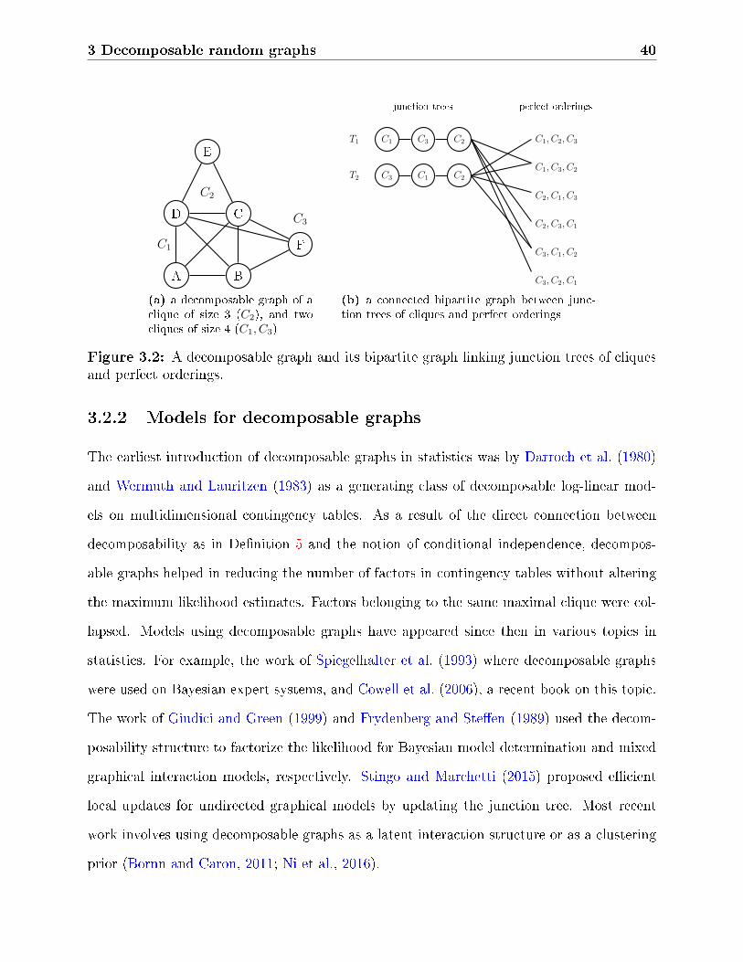
3 Decomposable random graphs 40

A B

CD

E

FC1

C2

C3

(a) a decomposable graph of aclique of size 3 (C2), and twocliques of size 4 (C1, C3)

C1 C3 C2

C3 C1 C2

C1, C2, C3

C1, C3, C2

C2, C1, C3

C2, C3, C1

C3, C1, C2

C3, C2, C1

T1

T2

junction trees perfect orderings

(b) a connected bipartite graph between junc-tion trees of cliques and perfect orderings

Figure 3.2: A decomposable graph and its bipartite graph linking junction trees of cliquesand perfect orderings.

3.2.2 Models for decomposable graphs

The earliest introduction of decomposable graphs in statistics was by Darroch et al. (1980)

and Wermuth and Lauritzen (1983) as a generating class of decomposable log-linear mod-

els on multidimensional contingency tables. As a result of the direct connection between

decomposability as in Denition 5 and the notion of conditional independence, decompos-

able graphs helped in reducing the number of factors in contingency tables without altering

the maximum likelihood estimates. Factors belonging to the same maximal clique were col-

lapsed. Models using decomposable graphs have appeared since then in various topics in

statistics. For example, the work of Spiegelhalter et al. (1993) where decomposable graphs

were used on Bayesian expert systems, and Cowell et al. (2006), a recent book on this topic.

The work of Giudici and Green (1999) and Frydenberg and Steen (1989) used the decom-

posability structure to factorize the likelihood for Bayesian model determination and mixed

graphical interaction models, respectively. Stingo and Marchetti (2015) proposed ecient

local updates for undirected graphical models by updating the junction tree. Most recent

work involves using decomposable graphs as a latent interaction structure or as a clustering

prior (Bornn and Caron, 2011; Ni et al., 2016).

3 Decomposable random graphs 41

The relative wide use of decomposable graphs stems from the separation property of

cliques and separators, which leads to a partitioning of the likelihood. In particular, Dawid

and Lauritzen (1993) have showed that, if, and only if, a random variable X = (Xi)i<n with

a Markov distribution p and a conditional dependency abiding to a decomposable graph G,

then the likelihood factorizes as

p(X | G) =∏

C∈C p(XC)∏S∈S p(XS)

, (3.2)

where C and S are the sets of maximal cliques and minimal separators, respectively, and

XA = Xi : i ∈ A.

Despite the broad use of decomposable graphs in statistics, little work has been done on

the sampling aspect. The lack of sampling methods is party due to the complexity of testing

for decomposability in large graphs, for example the size of the largest maximal clique is still

an open problem. In addition, it is partly due to the lack of explicit methods that generate

and quantify the space of junction trees or perfect orderings associated with a given graph.

The recent notable work of Thomas and Green (2009) and Stingo and Marchetti (2015)

take a steps in this direction, where both focus on updating the junction tree for faster

mixing time. Nonetheless, computational complexity is still the largest obstacle. As noted

by Thomas and Green (2009), one of the best available clique tree search algorithms is by

Tarjan and Yannakakis (1984), which is of the order O(|Θ|+|E|). Yet, for most dense graphs

|E| is of the order O(|Θ|2), and at best O(|Θ|) for sparse graphs.

This work adopts a more general modelling objective, where decomposable graphs are

seen as special cases of random graphs, in the sense discussed in Sections 2.2.3 and 2.2.5 and

surveyed in Orbanz and Roy (2015). Much of earlier work on decomposable graphs focused

on its junction tree representation, for its simplicity and computational eciency. The next

section introduces a model for decomposable random graphs that also builds on the junction

tree representation.

3 Decomposable random graphs 42

3.3 Decomposable random graphs by conditioning on junc-

tion trees

By denition, the building blocks of decomposable graphs are their maximal cliques and the

set of minimal separators. The smallest possible clique is a complete graph on two nodes (a

stick). For our modelling purpose, we will regard the smallest possible clique to be an isolated

node, where two isolated nodes form two maximal cliques, and connected they form a single

maximal clique. Hence, an n-node graph can have a maximum n maximal cliques, where

all nodes are isolated, and a minimum of one single clique, where all nodes are connected

forming an n-complete graph.

Relating the number of nodes to the range of possible cliques reects the fact that cliques

could be seen as latent communities which are observed in the clique form by the attainment

of node memberships. A decomposable graph is then an interaction between two sets of

objects, the graph nodes and the latent communities. In the discrete case, when the number

of nodes is known, out of the n-possible communities of an n-node graph, only 1 ≤ k ≤

n communities are observable in the form of maximal cliques. The rest of n − k clique-

communities are either latent with no visible node members or subgraphs of maximal cliques,

either way they are unobservable.

Let G be a decomposable graph with TG being one of its junction trees. In classical

settings, G is modelled via its adjacency matrix and TG is a function of G, and research

interest is in modelling the probability of node interactions.

Classical representation:

Given: G = (Θ, E) TG = f(G), interest: P(θi, θj ∈ E). (3.3)

This work models decomposable graph via their biadjacency matrix. By separating the

notion of nodes and maximal cliques, the biadjacency matrix connects the graph nodes to

3 Decomposable random graphs 43

the latent community nodes representing maximal cliques. Let θ′1, θ′2, · · · ∈ Θ′ be a set of

latent communities connected via the tree T = (Θ′, E), we dene Z to be the biadjacency

matrix of a decomposable graph G, where zki = 1 implies node θi is a member of clique θ′k,

otherwise zki = 0. In essence, Z represents a bipartite interactions between the two sets, Θ′

and Θ, such that θ′k, θi ∈ EZ , the Z edge set, also implies that node θi is a member of

clique θ′k. The interest is in modelling the probability of node-clique interactions.

Alternative representation:

Given: G = (Θ, E) T = (Θ′, E), Z =(Θ′,Θ, EZ

)interest: P(zki = 1). (3.4)

G is a deterministic function of Z, since its adjacency matrix is

A = (aij)ij =(minz⊺.iz.j , 1

)ij, (3.5)

where z.i is the i-th column of Z. Essentially, members of the same community, a row in Z,

are connected in G.

This assumes that an observed junction tree TG of G is, in some way, a subtree of T ,

since the maximal cliques C of G are a subset of Θ′. A more precise relation is TG = f(T ), as

function of T ; as a subtree when T (C) is a fully connected tree, that is, when all community

nodes representing maximal cliques are connected, with no sub-maximal nodes in between.

To fully capture the dynamics in decomposable graphs, a model for Z ought to be it-

erative, rst by modelling Z | T and iteratively T | Z. Classical models for decomposable

graphs, such as the work of Green and Thomas (2013), adopt a similar tree-dependent it-

erative scheme, where the conditional T update relies upon the bipartite relation in Figure

3.2, between trees and perfect orderings. This work models T | Z in a similar manner, thus,

the focus is proposing a model for Z | T .

Sampling edges in a decomposable graph is highly dependent on the current conguration

of the graph. Otherwise, (dis)connecting an arbitrary edge might hinder the graph unde-

3 Decomposable random graphs 44

composable. Figure 3.3 illustrates an example where a decomposable graph in 3.3a stays

decomposable in 3.3b, when node E joins clique AD, though with a dierent junction tree.

It becomes non-decomposable in 3.3c, when node F joins clique ABC, thus forming the circle

ADEF with no inner chord.

A

B

C

D

E

F

G

graph

junction treeABC AD DE EFG

(a) decomposable graph

A

B

C

D

E

F

G

graph

junction treeABC ADE EFG

(b) decomposable graphwith dierent junction tree

A

B

C

D

E

F

G

graph

(c) non-decomposable graph

Figure 3.3: An example of arbitrary adding an edge between nodes in a decomposablegraph: on the left is the original graph, in the middle, node E joins clique AD causing achange in the junction tree while preserving decomposability, on the right, node F joinsclique ABC, abolishing decomposability by forming the circle ADEF with no inner chord.

The Markov local dependency in decomposable graphs, shown in Figure 3.3, translates

directly to the biadjacency representation Z. Given T , sampling zki is highly dependent

on the current conguration of Z, that includes the current conguration of zki. Green

and Thomas (2013) have illustrated conditional (dis)connect moves on G | T that ensures

decomposability. The following proposition illustrates the permissible moves in Z | T that

ensures Z maps to a decomposable graph through (3.5).

Remark. The notation θ′k indexes the nodes of Z, it also represents the tree nodes in T .

To avoid ambiguity, let the term "node(s)" refer to the graph nodes, and "clique-node(s)"

to the nodes of the latent clique communities of Θ′ in the given tree T , unless otherwise

specied. For simplicity, we will often use the term "clique θ′k" to refer to the maximal

clique represented by the tree node θ′k, having the shorthand notation G(θ′k).

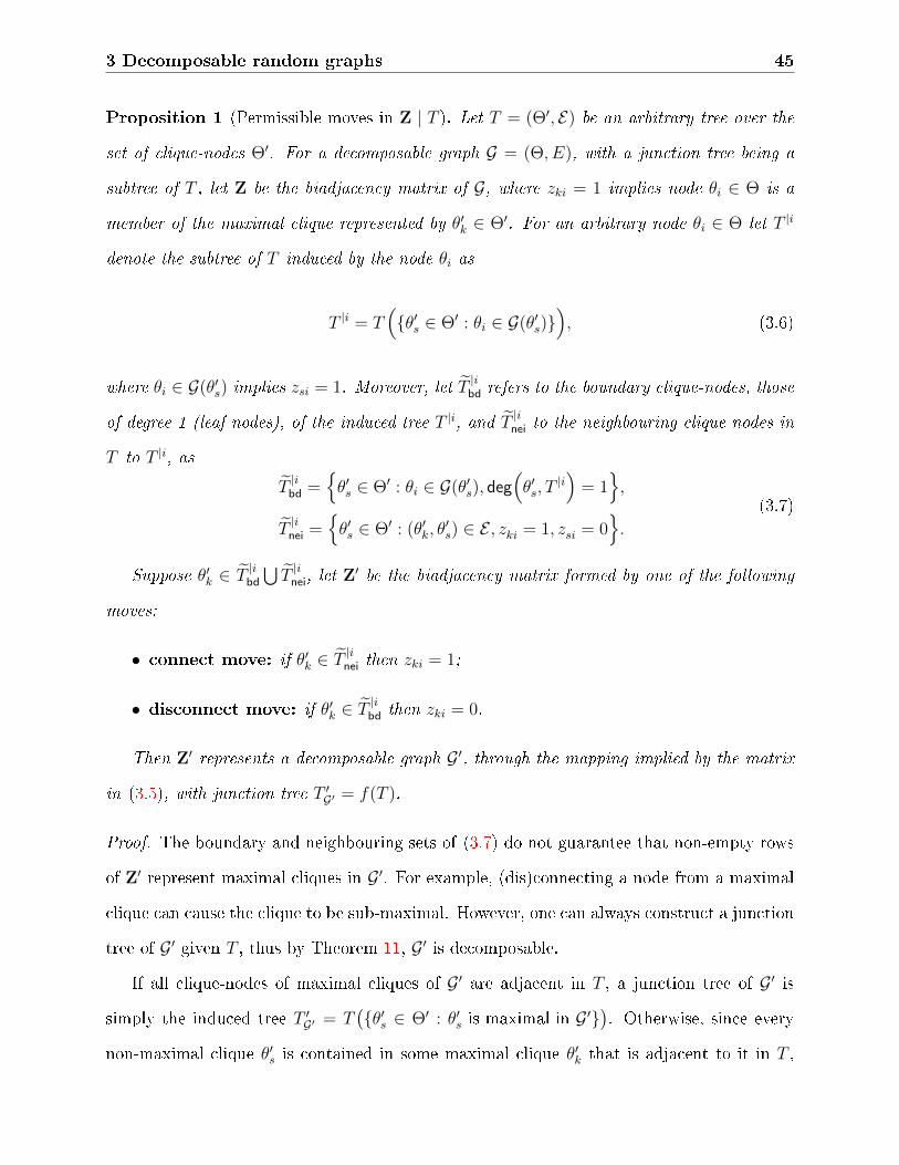
3 Decomposable random graphs 45

Proposition 1 (Permissible moves in Z | T ). Let T = (Θ′, E) be an arbitrary tree over the

set of clique-nodes Θ′. For a decomposable graph G = (Θ, E), with a junction tree being a

subtree of T , let Z be the biadjacency matrix of G, where zki = 1 implies node θi ∈ Θ is a

member of the maximal clique represented by θ′k ∈ Θ′. For an arbitrary node θi ∈ Θ let T |i

denote the subtree of T induced by the node θi as

T |i = T(θ′s ∈ Θ′ : θi ∈ G(θ′s)

), (3.6)

where θi ∈ G(θ′s) implies zsi = 1. Moreover, let T|ibd refers to the boundary clique-nodes, those

of degree 1 (leaf nodes), of the induced tree T |i, and T|inei to the neighbouring clique-nodes in

T to T |i, as

T|ibd =

θ′s ∈ Θ′ : θi ∈ G(θ′s), deg

(θ′s, T

|i)= 1,

T|inei =

θ′s ∈ Θ′ : (θ′k, θ

′s) ∈ E , zki = 1, zsi = 0

.

(3.7)

Suppose θ′k ∈ T|ibd

⋃T

|inei, let Z

′ be the biadjacency matrix formed by one of the following

moves:

• connect move: if θ′k ∈ T|inei then zki = 1;

• disconnect move: if θ′k ∈ T|ibd then zki = 0.

Then Z′ represents a decomposable graph G ′, through the mapping implied by the matrix

in (3.5), with junction tree T ′G′ = f(T ).

Proof. The boundary and neighbouring sets of (3.7) do not guarantee that non-empty rows

of Z′ represent maximal cliques in G ′. For example, (dis)connecting a node from a maximal

clique can cause the clique to be sub-maximal. However, one can always construct a junction

tree of G ′ given T , thus by Theorem 11, G ′ is decomposable.

If all clique-nodes of maximal cliques of G ′ are adjacent in T , a junction tree of G ′ is

simply the induced tree T ′G′ = T

(θ′s ∈ Θ′ : θ′s is maximal in G ′

). Otherwise, since every

non-maximal clique θ′s is contained in some maximal clique θ′k that is adjacent to it in T ,

3 Decomposable random graphs 46

θ′s, θ′k ∈ E , then all edges in T , except θ′s, θ′k, can be rewired to θ′k. This process forms

the tree T ′ where all maximal clique-nodes are adjacent and non-maximal clique-nodes are

leaf nodes. A junction tree T ′G′ is then the induced tree on T ′ as T ′

G′ = T ′(θ′s ∈ Θ′ :

θ′s is maximal in G ′).

The boundary and neighbouring sets in (3.7) of Proposition 1 do not ensure that cliques

remain maximal after a (dis)connect move in Z. For such cliques to remain maximal, we

impose extra conditions on both T|ibd and T

|inei. In the case of T

|ibd, we impose the extra

condition that a boundary clique stays maximal after a node's disconnection. Similarly, for

the case of T|inei, we impose the extra condition that a neighbouring clique stays maximal

after a node's connection. Formally, with abuse of notation, let T|ibd and T

|inei be as in (3.7),

though with the extra imposed conditions as

T|ibd = T

|ibd

⋂θ′k ∈ Θ′ : θ′k \ θi ⊈ θ′s, s = k

,

T|inei = T

|inei

⋂θ′k ∈ Θ′ : θ′k ∪ θi ⊈ θ′s, s = k

,

(3.8)

where θ′k \ θi refers to the subgraph formed by disconnecting the node θi from clique θ′k,

θ′k ∪ θi refers to opposite, the subgraph formed by connecting node θi to clique θ′k.

The extra imposed conditions in (3.8) are arguably restrictive and computationally ex-

pensive in large graphs, however, for a coherent introduction to the model, we will retain

these conditions. Section 3.3.2 examines a related issue, in which a practical solution is

proposed that also soften these conditions.

Proposition 1 illustrated the permissible moves in Z that ensures its representability as

a biadjacency matrix of a decomposable graph. The next section introduces a model for

random decomposable graph as realization from a continuous-time point processes in R2+.

3 Decomposable random graphs 47

3.3.1 Decomposable graph as point processes.

Drawing from the point process representation of graphs in Sections 2.2.4 and 2.2.5, let

(θi, ϑi) (θ′i, ϑ′i) be unit rate Poisson process on R2

+ representing the set of nodes Θ and

clique-nodes Θ′, respectively. Refer to θ as the node location and ϑ as the node weight.

Given a tree T = (Θ′, E), the biadjacency matrix Z, takes the form of a bipartite atomic

measure on R2+, as

Z =∑k,i

zkiδ(θ′k,θi), (3.9)

where zki := IUki ≤ W (α, ϑ′k, ϑi), for some random variable α ∈ R+, a uniform random

array (Uki) on [0, 1], and a random measurable function W : R3+ ↦→ [0, 1]. The decomposable

graph G represented by Z is then characterized as

G =∑i,j

min(∑

k

zkizkjδ(θ′k,θi)δ(θ′k,θj), 1)δ(θi,θj), (3.10)

Again G is completely determined by Z. The following denitions introduce useful graph

functions and notations used in this work.

Denition 6. Denote the operators v and e as node and edge sets of graph like structures,

respectively. Such that, v(G(x)) ∈ Θ are the nodes of the subgraph G(x), and e(G(x)) ∈ E

are the edges. Since Z also represents a bipartite graph, let v(Z(y)) be the subset of nodes and

clique-nodes in Θ′ ∪ Θ for the subgraph Z(y), and e(Z(y)) are the node-clique membership

edges. To distinguishing between nodes and clique-nodes in Z, denote vn(Z(y)) := v(Z(y)) \

Θ′ as the set of graph nodes , and vc(Z(y)) := v(Z(y)) \ Θ as the set of clique-nodes. For

the subtree T (t), v(T (t)) ∈ Θ′ and e(T (t)) ∈ E.

Denition 7. Following the notation Denition 6, denote nei as the operator of the set

of neighbouring nodes, and deg as the number of degrees for a specic node, respectively.

Such that nei(θi,G) are the neighbouring nodes of θi in G and deg(θi,G) = |(nei(θi,G)| is the

node degree. The junction tree follows similarly. For Z, nei(θi,Z) = vc(Z( . ∩ θi)

)and

3 Decomposable random graphs 48

nei(θ′k,Z) = vn(Z(θ′k ∩ . )

).

Given the characterization of neighbouring and boundary cliques (Eq. (3.8)), and the

characterization of zki in (3.9), we can accurately dene the n + 1 Markov update step for

z(n+1)ki given the current conguration Z(n), as

P(z(n+1)ki = 1 | Z(n), T ) = W (n+1)(ϑ′

k, ϑi) =

⎧⎪⎪⎪⎪⎪⎪⎪⎪⎪⎪⎨⎪⎪⎪⎪⎪⎪⎪⎪⎪⎪⎩

0 if z(n)ki = 0 and θ′k /∈ T

(n)|inei ,

1 if z(n)ki = 1 and θ′k /∈ T

(n)|ibd ,

W (ϑ′k, ϑi) if z

(n)ki = 1 and θ′k ∈ T

(n)|ibd ,

W (ϑ′k, ϑi) if z

(n)ki = 0 and θ′k ∈ T

(n)|inei .

(3.11)

Note that θ′k ∈ T(n)|ibd at step n only if θi is a member of the clique θ′k, that is z

(n)ki = 1.

Similarly, θ′k is a neighbour to T (n)|i only if z(n)ki = 0. Otherwise, as in the rst and second

case in (3.11), z(n+1)ki = z

(n)ki . Then, (3.11) simplies to

P(z(n+1)ki = 1 | Z(n), T ) = W (n+1)(ϑ′

k, ϑi) =

⎧⎪⎪⎨⎪⎪⎩W (ϑ′

k, ϑi) if θ′k ∈ T(n)|ibd

⋃T

(n)|inei ,

z(n)ki otherwise.

(3.12)

For simplicity, W is specied in (3.11) and (3.12) with its last two arguments relating to

the weight parameter of the nodes and clique-nodes. Nonetheless, the form of W in (3.12)

is still unspecied, and for it to be a sensible modelling object, the most general denition

would require it to be at least measurable with respect to a probability space. Depending on

the sampling method, more conditions might be required. Notably, the framework used thus

far mimics that of the Kallenberg representation theorem as introduced in Section 2.2.5. A

realization from such a random innite measure is seen as cubic [0, r]2, r > 0, truncation of

R2+, and in that sense, the point process on the nite region [0, r]2 might not be nite. In

practice, a realization from a nite restriction is desired to be nite. Kallenberg (2005, Prop.

9.25) has given necessary and sucient conditions for an exchangeable measure to be a.s.

3 Decomposable random graphs 49

locally nite. Since we are not particularly focused on exchangeable random measures, yet

still interested in the niteness of a realization, the following denition simplies Kallenberg's

condition by taking the random functions S = S ′ = I = 0 in Section 2.2.5.

Denition 8. (locally nite) Let ξ be a random atomic measure on R2+, such that for a

measurable random function W : R3+ ↦→ [0, 1], ξ takes the form

ξ =∑i,j

IUij ≤ W (α, ϑ′i, ϑj)δ(θ′i,θj),

where (θ′i, ϑ′i) and (θj, ϑj) are two independent unit rate Poisson processes on R2

+, and

(Uij) is a [0, 1] uniformly distributed 2-array random variables. Then for a xed α, the

random measure ξ is a.s. locally nite if, and only if, the following conditions are satised:

(i) ΛW 1 = ∞ = ΛW 2 = ∞ = 0,

(ii) ΛW 1 > 1 <∞ and ΛW 2 > 1 <∞,

(iii)∫R2+W (x, y)IW 1(y) ≤ 1IW 2(x) ≤ 1dxdy <∞,

where W 1(y) =∫R+W (x, y)dx and W 2(x) =

∫R+W (x, y)dy, and Λ is the Lebesgue measure.

In summary, if W is integrable then ξ is a.s. locally nite.

Thus far, we have introduced the general framework of the proposed model, the Markov

update scheme at each step, and the required conditions on W to ensure a nite realization

of the model. We will now give a formal denition of decomposable random graphs.

Denition 9 (Decomposable random graph). A decomposable random graph G, is a random

graph associated with a biadjacency atomic random measure Z taking the form in (3.9), with

the random function W : R3+ ↦→ [0, 1] satisfying the conditions in Denition 8, where Z is

constructed by means of a Markov process having the update steps of (3.12). A realization

of such measure also takes the form of an (r′, r)-truncation as Zr′,r = Z( . ∩ [0, r′] × [0, r]),

for r′, r > 0.

3 Decomposable random graphs 50

The denition of random decomposable graphs in 9 specied the Markov update process

of (3.12), which itself depends on the boundary and neighbouring sets of (3.8). Instead, the

simpler boundary and neighbouring sets of (3.7) could be used, since as shown in Proposition

1, a formation of Z using the sets in (3.7) would result in a decomposable graph by the

mapping of (3.10). However, in this case, the latent tree T connecting the clique-nodes

(θ′k, ϑ′k) would not be seen as the limit of a junction tree of the graph as more nodes enter

the truncation. A direct result from the fact that the clique-nodes in T can represent both

maximal and non-maximal cliques under (3.7). Thus treatment of decomposable graphs is

possible, in Chapter 4 we showcase an application resulting from such treatment, where we

treat sub-maximal cliques as sub-clusters of maximal cliques.

The sampling notion of an (r′, r)-truncation mentioned in Denition 9 is not yet fully

discussed, in particular, how it assures decomposability with scaling of r or r′. The next

section formalizes this notion, where certain issues relating to decomposability are disclosed

with some proposed solutions.

3.3.2 Finite graphs forming from domain restrictions

Having made the choice of representing the biadjacency matrix Z as an innite point process

on R2+, then, a nite observation of Z can be seen as the graph resulting from the cubic

restriction [0, r′]× [0, r] of R2+, where clique-nodes and nodes are visible only if they appear

in some edge in Zr′,r = Z( . ∩ [0, r′]× [0, r]), with locations satisfying that θ′k < r′ and θi < r.

In this case, refer to the appearing clique-nodes and nodes as active.

There is a clear ambiguity relating to the inuence of each domain restriction on the

other, specially due the Markov formation of the graph. Nonetheless, if we neglect for a

moment the formation method, and regard the biadjacency Z to be an innite xed object

sampled by the (r′, r)-truncation as Zr′,r, there is still doubt on how an achieved realization

forms a decomposable graph. For example, a random embedding of clique-node locations

θ′1, θ′2, . . . in R+ can result in an empty realization even for large values of r′, inuenced

3 Decomposable random graphs 51

by the inter-dependence between clique-nodes in T . Essentially, what is required is that a

realization from Zr′,r is decomposable with a junction tree as a function or subtree of T , albeit

not necessary completely connected. In fact, the observable part of T forms a collection,

perhaps connected, of parts of the junction tree parameterizing the graph mapped from

Zr′,r. Even if such notion is allowed, there is still no promise that all active clique-nodes in

a realization is a maximal clique, since a visible portion of a clique, where part is located

outside the truncation, might be contained in another clique within the truncation. A simple

way to address those two issues is to ensure that the restriction point r is magnitudes larger

than r′, to allow enough active nodes such that all active clique-nodes are maximal. Gauging

the truncation size can be done be ensuring that the following A0 set is empty.

A0θ′k < r′ : Zr′,r(θ′k ∩ . ) ⊆ Zr′,r(θ′s ∩ . ), for some θ′s < r′, s = k, θ′k is active

= ∅. (3.13)

Note that θ′s need not be active in (3.13), as for non-active cliques Zr′,r(θ′k ∩ . ) =

∅. Essentially, the conditions in A0 are the same conditions added to the boundary and

neighbouring sets in (3.8).

To scale freely the (r′, r)-truncation, while ensuring A0 is empty, one can, extend the

truncated location node domain by an "edge-greedy" partition (r, ro] as [0, r]∪ (r, ro]. Rather

than trimming all external edges connecting from (r, ro] to [0, r′], as done with edges outside

the cube [0, r′] × [0, r], we only allow a maximum of a single edge per node θi ∈ (r, ro]

to connect to any active clique-node θ′k ∈ [0, r′], only if it causes Zr′,ro(θ′k ∩ . ) to be

maximal if it was not in Zr′,r(θ′k ∩ . ). In other words, let e(Zr′,r) be the edge set formed

in Zr′,r, then |e(Zr′,ro(θi ∩ .))| ≤ 1, for each r < θi ≤ ro, and (θ′k, θi) ∈ e(Zr′,ro) only

if Zr′,r(θ′k ∩ . ) ⊆ Zr′,r(θ′s ∩ . ) for some θ′s, θ′k ≤ r′, k = s. Figure 3.4 illustrates this

process from a realization of a decomposable graph using the restrictions [0, r′]× [0, r] with

the edge-greedy partition (r, r0], where one extra node, θ∗, is included to clique θ′3 to insure

the set in (3.13) is empty.

Remark. Allowing r to be much larger than r′ relates directly to the notion discussed at the

3 Decomposable random graphs 52

beginning of Section 3.3, that the set of maximal cliques of T are only partially observable

given the nodes.

θ

θ'

θ1θ2 θ3θ4θ5 θ6 θ7 θ8 θ9

θ 1'

θ 2'

θ 3'

θ 4'

θ 5'θ

6'θ 7

'

r

r'

ro

(a) graph as a point process

(b) latent tree T

sampled biadjacency matrix

θ′ θ

7654321

1 2 3 4 5 6 7 8 9 *blue node

(c) sampled and extended biadjacency matrix

2

5 3 4

67

1

8

9

*

(d) mapped decomposablegraph

Figure 3.4: A realization of a decomposable graph in 3.4d from the point process in 3.4a andthe tree 3.4b. The grey area in 3.4a is the edge-greedy partition (r, ro], where only one extranode (in blue) was needed to guarantee all active cliques are maximal, since Zr′,r(θ′3 ∩ .)is a subset of Zr′,r(θ′6 ∩ .) and Zr′,r(θ′7 ∩ .). 3.4c is the biadjacency matrix of active(clique-)nodes representing the graph.

Condition A0 is not such a computational burden given the biadjacency representation,

since one can compare the o-diagonal to the diagonal entries of Zr′,rZ⊤r′,r, to arrive at where

3 Decomposable random graphs 53

to allow an edge in the edge-greedy partition. In a graph of Nc active clique-nodes, A0

checks each of the Nc clique-nodes with their neighbours, thus for a d-regular junction tree,

where all clique-nodes are of degree d, the computational complexity is of a linear order as

O(dNc). Nonetheless, a simpler solution is possible by an identity matrix augmentation, as

shown in the next subsection

3.3.2.1 Augmentation by an identity matrix

To avoid such unnecessary checks in A0, one can simply augment a realization by an identity

matrix, after the removal of empty rows, as per the Kallenberg representation of random

graphs. In essence, this operation articially adds a maximum Nc extra nodes to the graph,

each node is connected to a single unique clique, thus uniquely index the clique set. This

process is summarized in Figure 3.5, with the removal of empty rows and an identity aug-

mentation to the realization in Figure 3.4c. Such augmentation, though it seems articial, is

a natural consequence of the used framework and the edge-greedy partition. In a sense, given

the (r′, r)-truncation method, for any realization over Zr′,r, with probability 1, there exists

an ro > r such that the edge-greedy partition (r, ro] embeds an identity matrix. To show

this, we will extend the results of Veitch and Roy (2015) concerning the degree distribution

of the Kallenberg exchangeable graph discussed in Section 2.2.5, to the case of a biadjacency

measure.

Consider the random biadjacency atomic measure generated using the Kallenberg repre-

sentation and taking the following simplied form

G =∑k,i

IUki ≤ W (α, ϑ′k, ϑi)δ(θ′k,θi), (3.14)

where all notations and conditions follow that of Denition 8. A realization from G is also

an (r′, r)-truncation as Gr′,r = G( . ∩ [0, r′] × [0, r]) where only edge-connected nodes are

visible. The construction of G diers from that of the decomposable graph in Denition 9,

3 Decomposable random graphs 54

reduced clique-node matrix

θ′ θ

7631

1 2 3 4 5 6 7 8 9 * * * *

identity

(a) augmented clique-node bipartite matrix.

2

5

*

3 4

67

*

1

8

9*

*

(b) mapped decomposablegraph

Figure 3.5: Relaxation of (3.13) by removing the empty rows in the realization of Figure3.4c and augmenting the results with an identity matrix.

where the latter is conditioned on a latent tree structure while the former is not. Given a

realization Gr′,r, we then can dene the degree distribution of any point in the domain of

the x-truncated Poisson process Πx, or any of the two domains by symmetry. Let

deg((θ, ϑ),Πr,Π′r′ , (Uij)), (3.15)

be the degree of the point (θ, ϑ) in the domain of Πr conditioned that (θ, ϑ) ∈ Πr. However,

the probability that (θ, ϑ) ∈ Πr is 0, thus as noted by Veitch and Roy (2015) and discussed

more generally in Chiu et al. (2013), this conditioning is ambiguous and ill formulated.

Nonetheless, a version of the required conditioning can be obtained by the Palm theory of

measures on point sequences. The Slivnyak-Mecke theorem states that the distribution of a

Poisson process Π conditioned on a point x is equal to the distribution of Π ∪ x; with

this we characterize the degree distribution in the following lemma.

Lemma 1. For a biadjacency measure Gr′,r, dened in (3.14), with a non-randomW : R2+ ↦→

[0, 1] and a xed α, the degree distribution of a point (θ, ϑ) ∈ R2+, θ < r, is deg((θ, ϑ),Πr ∪

(θ, ϑ),Π′r′ , (Uki))

d∼ Poisson(r′W 1(ϑ)), and by symmetry of construction, deg((θ′, ϑ′),Π′r′ ∪

(θ′, ϑ′),Πr, (Uki))d∼ Poisson(rW 2(ϑ

′)).

3 Decomposable random graphs 55

Proof. Since (θ, ϑ) ∈ Πr with probability 0, then using the Palm theory we have

deg((θ, ϑ),Πr ∪ (θ, ϑ),Π′r′ , (Uki)) =

∑(θ′k,ϑ

′k)∈Π

′r′

IUθ′k,θ ≤ W (ϑ′k, ϑ). (3.16)

By Denition 8, W is a.s. nite, thus by a version of Campbell's theorem (Kingman,

1993, ch 5.3), the characteristic function of (3.16) is

E[exp

(itdeg

((θ, ϑ), .

))]= exp

(∫R+

∫[0,1]

(1− eitIu≤W (x,ϑ))r′dudx)

= exp(r′W 1(ϑ)(e

it − 1)),

(3.17)

where W 1(y) =∫R+W (x, y)dx. The results follows similarly for the second domain. For a

random W , the same results can be achieved by conditioning.

Now that the degree distribution in Gr′.r is well dened, we can now show that the

identity matrix augmentation, in Figure 3.5, is a natural consequence.

Proposition 2. For a realization over Zr′,r from a biadjacency measure as Dened in 9, let

Θ′r′ be the nite set of active clique-nodes in Zr′,r, where |Θ′

r′ | > 1. Then, with probability

1, there exists an ro > r, such that each θ′k ∈ Θ′r′ is indexed by a unique node r < θπ(i) < ro

that is not connected to any other active clique-node. Thus, the partition (r, ro] embeds an

identity matrix.

Proof. Given a realization over Zr,′r, index the almost surely nite set of active clique-nodes

as θ′1, θ′2, . . . ,∈ Θ′

r′ . For t > 0, let

Y(k)t = |e(Zr′,r+t(θ′k ∩ . ))| − |e(Zr′,r(θ′k ∩ . ))|

= deg((θ′k, ϑ′k),Π

′r′ ,Πr+t, (Uki))− deg((θ′k, ϑ

′k),Π

′r′ ,Πr, (Uki)),

as the degree of the k-th active clique θ′k ∈ Θ′r′ over the partition (r, r + t]. For a nite t,

Y(k)t is an almost surely non-negative nite process, by niteness of the generating measure

(Denition 8). For the ltration F := σ(α, (θ′k, ϑ′k), T ), dene τ (k) to be the stopping time

3 Decomposable random graphs 56

of the event that an edge appears between a node in a unit interval and θ′k, while no edge in

the same interval appears for the rest of the active clique-nodes. Formally,

τ (k) := mint ∈ N : Y (k)

t+1 − Y(k)t > 0

⋂s =k

Y (s)t+1 − Y

(s)t = 0, θ′s ∈ Θ′

r′

. (3.18)

Then, it suces to show that τ (k) <∞ with probability 1 for each θ′k ∈ Θ′r′ and then take

ro = maxk(τ(k)). By conditioning on the latent tree, (Y

(k)t )k are not independent and do not

yield an accessible distribution. Nonetheless, if we let (Y(k)t )k represent the analogous process

though under the standard biadjacency measure of (3.14), then (Y(k)t )k are independent with

a well dened distribution (Lemma 1). Moreover, for each k, Y(k)t is dominated by Y

(k)t as

Y(k)t ≤ Y

(k)t , since the latter could be seen as induced by an innite complete graph KG,

where T ⊂ KG. For an analogous ltration F := σ(α, (θ′k, ϑ′k), KG), and the stopping time

τ (k) under (Y(k)t )k we have

P(τ (k) ≥ n) ≤ P(τ (k) ≥ n) ≤ 1

nE[τ (k) | F ]

=1

nE[∑t≥1

tIs < t : s = τ (k)Iτ (k) = t | F]

≤ 1

n

∑t≥1

t[ t−1∏i=1

1−P(Y

(k)i+1 − Y

(k)i > 0

)P(⋂s =k

Y (s)i+1 − Y

(s)i = 0

)]

≤ 1

n

∑t≥1

t

[1− exp

(−∑s =k

W 2(ϑ′s))]t−1

=1

nexp

(2∑s =k

W 2(ϑ′s))−→ 0 as n −→ ∞.

The inequalities above are a result of the Markov inequality, the independence of (Y(k)t )k,

the removal of the rst probability in the third line, the direct application of the geometric

series sum, and nally by condition (i) in Denition 8. The proof could be also achieved via

the Borel-Cantelli Lemma.

This section formalized the notion of a realization from a decomposable random graph

3 Decomposable random graphs 57

of Denition 9 through the means of an (r′, r)-truncation. A realization with active non-

maximal cliques, if it occurs, can be corrected by an edge-greedy partition to fulll condition

A0 (E.q. (3.13)), or by an identity matrix augmentation, where the latter happens with

probability 1 for a xed set of active clique-nodes and an ro < ∞. This section discussed

more generally the issues of post-generation embedding in R2+ while ignoring the Markovian

nature of the generation process. Section 3.4 lls the gap by illustrating a practical sampling

procedure of such a process, where the results of this section become useful. Meanwhile,

Section 3.3.2.2 demonstrates some interesting results relating to likelihood factorization in

terms of the Z representation.

3.3.2.2 Likelihood factorization with respect to Z

Denition 9 introduced decomposable random graph and a process forming through se-

quential Markov updates using (3.12). In (3.12) the restrictive boundary and neighbouring

induced-tree set of (3.8) were used to ensure every active clique-node in Z represents a

maximal clique in G. Otherwise, the simpler sets in (3.7) can be used.

In the eld of graphical models, decomposable graphs are used to factorize the likelihood

of multivariate distribution into a product of likelihoods over conditionally independent com-

ponents. This is illustrated in (3.2). An interesting question is whether one can factorize

the likelihood of a multivariate distribution, with conditional dependency abiding to a de-

composable graph G, with respect to its Z representation instead, and is this factorization

equivalent to one represented in (3.2)? If factorization is possible, do active non-maximal

clique-nodes inuence the factorization, in other words, can the sets (3.7) be used instead of

(3.8)?

Theorem 12 (Likelihood factorization with respecto to Z). Let Z be an Nc×Nv biadjacency

matrix generated from the Markov process (3.12) over the latent community tree T = (Θ′, E).

In (3.12), let the simpler boundary and neighbouring sets of (3.7) be used. Let G be the

decomposable graph generated from Z by (3.5) or (3.10), with junction tree TG. Moreover, let

3 Decomposable random graphs 58

X = (Xi)i<Nv be a random variable with a Markov distribution p and conditional dependency

abiding to G, then the likelihood of X | Z can be represented as

p(X | Z) =∏

θ′k∈Θ′ p(Xθk)∏θ′k,θ

′j∈E

p(Xθ′k∩θ′j). (3.19)

In fact, p(X | Z) = p(X | G) of (3.2).

Proof. Assuming that X∅ = ∅, such that p(X∅ = x∅ | Z) = 1, thus discarding all empty

clique-nodes from the numerator and denominator of (3.19). Since not all θ′k ∈ Θ′ are

maximal, we will show that every non-maximal clique in the numerator of (3.19) cancels out

with an equivalent factor in the denominator, leaving the minimal separator set S of G as in

(3.2).

Active clique-nodes that are not maximal can either be: i) on the path between two

maximal cliques; ii) on a boundary branch of T stemming out of a maximal clique.

For case i), let θ′k1 , θ′k2, . . . , θ′kn−1

be sub-maximal cliques on the bath between two maximal

cliques, θ′k0 and θ′kn, that are adjacent on some junction tree TG of G. Let S = θ′k0 ∩ θ′kn the

separator representing the edge θ′k0 , θ′kn in TG. It is straightforward to show that S ⊆ θ′ki

for all i = 1, . . . , n−1, otherwise the RIP is violated. There are n edges for n−1 sub-maximal

cliques-nodes in a path between two maximal cliques. For each of the sub-maximal cliques

θ′ki , i = 1, . . . , n− 1, by the RIP, either θ′ki ⊆ θ′ki−1, or θ′ki ⊆ θ′ki+1

, or both. If θ′ki ⊆ θ′ki−1then

p(Xθ′ki∩θ′ki−1

) = p(Xθ′ki), thus eliminating the same factor in the numerator of (3.19). The

opposite is true, when θ′ki ⊆ θ′ki+1. This process reduces the path to the single edge θ′k0 , θ′kn

representing S.

For case ii), all sub-maximal clique-nodes on a boundary branch of T stemming out of

a maximal clique, say θ′k0 , are contained in θ′k0 . By the RIP, all their edges can be rewired

to θ′k0 . The intersection in the denominator of (3.19) returns the sub-maximal factors as in

case i), hence eliminating them from the numerator.

The results of Theorem 12 enables one to use the faster mixing set of (3.7) in the Markov

3 Decomposable random graphs 59

update process without aecting the likelihood of interest. This enables specifying the a

multivariate distribution completely in terms of Z, avoiding the transformation to G.

3.4 Exact sampling conditional on a junction tree

Sampling from the proposed model could be done in multiple ways, primarily due to the

Markovian nature of decomposable graphs. This section illustrates two methods, one based

on a sequential procedure with nite number of steps, while the second adapts a Markov

update method, where samples are obtained from the stopped process. Nonetheless, both

methods overlap in the sampling and embedding of the Poisson process and the assignment

of clique-nodes, which is discussed below.

To sample a decomposable graph from an (r′, r)-truncation, let T = (Θ′, E) be an innite

tree with clique-nodes Θ′ = (θ′1, θ′2, . . . ). Thus far, only the location dimension of the used

Poisson process is considered in the (r′, r)-truncation. This risks innite values for the weight

dimension (ϑ). It is only natural to assume a Poisson process on the [0, r]× [0, c] cube, where

only points with θ < r and ϑ < c are kept. A standard generative model of nodes and their

location embedding can be:

Nv ∼ Poisson(cr),

(θi) | Nviid∼ Uniform[0, r],

(ϑi) | Nviid∼ Uniform[0, 1],

Nc ∼ Poisson(c′r′),

(θ′k) | Nciid∼ Uniform[0, r′].

(ϑ′k) | Nc

iid∼ Uniform[0, 1].

(3.20)

where Nv is the number of nodes and Nc is the number of clique-nodes.

The iterative sampling of T | Z is discussed in a later section, Section 3.5. This section

only samples a subtree of a given tree by adopting a random walk type of sampler of clique

3 Decomposable random graphs 60

edges, to avoid the high probability of disjoint components associated with random sampling.

The latter could be the case when the tree is known to be nite. The assignment process is

then:

θ′1 ≡ θ′σ(1),

θ′n+1 | θ′1, . . . θ′n ∼ Uniform(θ′k ∈ Θ′ : θ′k, θ′s ∈ E , s ≤ n

),

(3.21)

where σ(1) is a randomly selected clique-node as the root of the sampled tree, and the uniform

distribution samples from the neighbouring clique-nodes in Θ′ to the already assigned ones.

Recall that T (n)|i is the θi-induced subtree of T at the n-th Markov step, as dened

in (3.6), T(n)|ibd is the boundary clique-nodes and T

(n)|inei is the neighbouring clique-nodes, as

dened in (3.8). Note that all subtree quantities are dened prior to the (r′, r)-truncation,

thus, we are implicitly assuming that they abide to the condition that θ′k < r′, particularly

for T(n)|inei .

3.4.1 Sequential sampling with nite steps

Because of the dependency induced by T , and as discussed in Section 3.3.2, some nodes

might only connect to clique-nodes outside the (r′, r)-truncation (non-active). Then, for

i = 1, . . . , Nv, a node is active within the truncation proportional to the [c′, r′] truncation

total mass as:

θi is active | W, c′, ϑi ind∼W 1(c

′, ϑi)

W 1(ϑi), (3.22)

where W 1(c′, ϑ) =

∫ c′0W (x, ϑ)dx.

For each active θi sample edges as:

• sample the rst edge as

θ′π(k), θi | (ϑ′k),W

ind∼W (ϑ′

π(k), ϑi)

W 1(c′, ϑi). (3.23)

3 Decomposable random graphs 61

• at the (n+ 1) step, sample edges to neighbouring clique-nodes sequentially as

θ′π(n+1) | (θ′π(k))k≤n ∼ Uniform(T

(n)|inei \ (θ′π(k))k≤n

),

θ′π(n+1), θi | ϑ′π(n+1), ϑi,W ∼ Bernoulli

(W (ϑ′π(n+1), ϑi)

W 1(c′, ϑi)

).

(3.24)

3.4.2 Sampling using a Markov stopped process

A Markov chain sampling of decomposable graphs depends on a stopped process, where a

Markov chain is run and a realization is obtained by stopping the chain at a specic time.

Such a process is slower in nature than the sequential sampling process discussed in the

previous section. In principle, one samples edges uniformly and decides whether they appear

at the current step given the current conguration of the biadjacency matrix. For the n+ 1

Markov step, sample edge indices uniformly as

k | Nciid∼ Uniform[1, . . . , Nc],

i | Nviid∼ Uniform[1, . . . , Nv].

(3.25)

Sample the θ′k, θi edge as

θ′k, θi | ϑ′k, ϑi,W, T ∼ Bernoulli

(W (ϑ′

k, ϑi) Iθ′k ∈ T(n)|ibd ∪ T (n)|i

nei ∪ χ(n)|i0

), (3.26)

with

χ(n)|i0 (θ′) =

⎧⎪⎪⎨⎪⎪⎩θ′ if |v(T (n)|i)| = 0

∅ otherwise.

(3.27)

A realization is then the result of stopping the above iterative process at a random time

t > 0. Ideally, the stopping time should be chosen after the Markov chain has reached

stationarity, such time is referred to as the mixing time of the Markov chain. The next

section gives a mixing time result on the Markov stopped process illustrated here.

3 Decomposable random graphs 62

3.4.2.1 Mixing time of the stopped process

For a precise denition of the mixing time, let Ω be a the state space of a Markov chain

(Xt)t≥0 with transition matrix P . Let P t(x, y) = P(Xt = y | X0 = x) for x, y ∈ Ω, be the

probability of the chain reaching state y in t-steps given it started at state x. Dene the

total variation distance d(t) between the transition matrix P t, at step t, and the stationary

distribution p as

d(t) := maxx∈Ω

∥ P t(x, .)− p ∥TV , (3.28)

where ∥ . ∥TV is the total variation norm. Then the mixing time tmix is dened as

tmix := mint > 0 : d(t) < 1/4. (3.29)

Variations of mixing times for other thersholds ϵ = 1/4 exits, though it is shown inde-

pendently that tmix(ϵ) ≤ [log2(ϵ−1)]tmix(1/4). Therefore, it suces to work with (3.29). For

an excellent introduction to Markov chain mixing times, refer to the book of Levin et al.

(2009).

For the proposed sampling method (E.q. (3.25) and (3.26)), a unique stationary distribu-

tion p exists, since by construction the chain is irreducible, that is for any two congurations

x, y ∈ Ω, P t(x, y) > 0 for some t ∈ N (Levin et al., 2009, Coro. 1.17, Prop. 1.19). Then, it

remains to nd a lower bound for tmix.

A known method to establish lower bounds for mixing times over irreducible Markov

chains is by bounding the probability of the rst time a coupling over the chain meets.

Given an irreducible Markov chain over a state space Ω, with transition probability P , a

coupling is a process of running two Markov chains (Xt)t and(Yt)t, with the same P , though

with dierent starting points. A coupling meets when the two chains visit a state at the

same time and move together at all times after they meet. More precisely,

if Xs = Ys, then Xt = Yt for t ≥ s. (3.30)

3 Decomposable random graphs 63

Theorem 13. (Levin et al. (2009, Theo. 5.2)) Let (Xt, Yt) be a coupling with transition

matrix P satisfying (3.30), for which X0 = x and Y0 = y. Let τcouple be the rst time the

chain meets:

τcouple := mint > 0 : Xt = Yt. (3.31)

Then

d(t) ≤ maxx,y∈Ω

Px,y(τcouple > t). (3.32)

An example of a coupling on an n-node rooted binary tree, is by taking two lazy random

walks (Xt, Yt), started at nodes X0 = x, Y0 = y, where at each step a fair coin decides

which chain to move. Then, uniformly move the chosen chain to a neighbouring node, while

keeping the other chain xed. Once the two chains are at the same level from the root node,

couple them by moving them further or closer to the root simultaneously. In this case, the

rst coupling time is less than the commute time (τ0,∂B), the time a chain commutes from

the root to the set of leaves ∂B and back. By τ0,∂B the coupling would have occurred.

Proposition 3. (Commute Time Identity (Levin et al., 2009, Prop. 10.6)) Given a nite

tree Tn with n nodes, a root node x0, and a set of leaves ∂B. Let τ0,∂B be the commute time

dened as

τ0,∂B := mint ≥ τ∂B : Xt = X0 = x0, Xτ∂B ∈ ∂B, (3.33)

for a random walk (Xt)t on Tn. Then

E[τ0,∂B] = 2(n− 1)∑k

1

Γx0k, (3.34)

where Γx0k is the number of nodes at distance k from the root.

Remark. The maximum commute time is attained for a lazy random walk on a straight line

(a path) tree with n nodes at each side of the root, where E[τ0,∂B] = 4n2. For a lazy random

3 Decomposable random graphs 64

walk with probability p that the chain stays at the same conguration, it is easy to see that

the expected commute time (3.34) becomes E[τ0,∂B]/p.

A similar approach could be applied to the proposed sampling scheme of (3.25) and

(3.26). First, note that sampling edges for a xed node θi depends on the conguration

of other nodes. This dependence is enforced by the extra conditions added to T(n)|ibd and

T(n)|inei in (3.8) versus (3.7). However, as discussed in Section 3.3.2, by using the edge-greedy

partition one can relax both of those conditions, either by satisfying A0 (E.q. (3.13)) using

the minimum amount of steps in post-sampling, or by an identity matrix augmentation as in

Figure 3.5. Moreover, (3.7) will still result in a decomposable graph, as shown by Proposition

1, though not all active clique-nodes are maximal.

The objective of breaking down the dependency between nodes is to reduce the problem

of studying the mixing time on the whole graph to studying it on each node independently,

over the given tree. In this case, the process in (3.26) does not map directly to a random

walk process, where we can apply the commute time identity. For three reasons: (i) for each

node θi, the edges of the junction tree are directional and weighted by W (ϑ′., ϑi); (ii) The

variable χ(n)|i0 in (3.27) acts like a transporting hub to a random clique-node whenever the

random walk returns to the starting position; (iii) The commute time in 3 depends on a

root node, that is not a property of the proposed sampling method. Nonetheless, all three

reasons can be handled. Reason (i), for a non-atomic W a uniform expected weight of

E[W ] =

∫∫R2+

W (x, y)dxdy, (3.35)

can be used. It is attained by a direct application of the Mapping theorem of (Kingman,

1993), as in Figure 3.6. Reason (ii), the transport hub property only speeds up the commute

time, thus an upper bound is still the commute time of (3.33). Reason (iii),∑

k 1/Γk

is smallest when the designated root node is the centre of the tree, where each side is

symmetric. It becomes larger as the designated root node moves away from the centre, with

3 Decomposable random graphs 65

the maximum of Lmax/2, half the maximum distance between two leaf nodes.

θ′1 θ′2

θ′3

θ′4 θ′5

W1

W2

W3

W1

W5

W3W

4

W3

θ′1 θ′2

θ′3

θ′4 θ′5

W∗

W∗

W∗W

∗

Figure 3.6: A realization of a 5-node junction tree from (3.21), on the left is the originaldirected weighted tree where Wk = W (ϑ′

k, ϑi) for a random ϑi, on the right is the undirectedtree by expectation where W∗ = E(W ).

Lemma 2. For the Markov update process of Section 3.4.2, given a connected tree with Nc

clique-nodes, the lower bound of the expected mixing time for each node, holding all other

nodes constant, is

tmix ≥8Nc∫∫

R2+W (x, y)dxdy

Lmax

2≥ 8Nc∫∫

R2+W (x, y)dxdy

Nc∑k=1

1

Γk, (3.36)

where Γk is number of nodes at distance k form a root node θ′0, selected randomly from the

non-leaf nodes of the tree, and Lmax is the maximum distance between two leaf clique-nodes.

If nodes are sampled independently, when (3.7) is used instead of (3.8), then (3.36) is the

global mixing time achieved by parallel sampling.

The proof follows directly from Theorem 13 and Proposition 3 by a lazy random walk

with probability as in (3.35).

3.5 Edge updates on a junction tree

Section 3.3 proposed a model for decomposable random graphs by conditioning on a xed

junction tree, where graph edges are formed conditionally through a Markov process, as

shown in (3.12) and Section 3.4. Nonetheless, conditioning the model on a xed junction

3 Decomposable random graphs 66

tress is quite restrictive for two main reasons: (i) the junction trees representation is not

unique; (ii) a junction tree is oftentimes unknown and an estimate is desired. Sampling

of junction trees is possible, for example, by single edge updates on the given tree. This

connection is summarized by Hara and Takemura (2006), through a connected bipartite

graph between the set of possible junction trees and the set of POSs, as shown in Figure 3.2.

Despite the non-uniqueness of junction tree and the POSs, Lauritzen (1996) has showed

that the set of minimal separators, edges of the junction tree, is unique with varying mul-

tiplicity for each separator. The separator multiplicity relates to the number of ways its

corresponding edge can be formed, and thus the number of trees that are a unit distance, or

a single move, away. Therefore, for two adjacent maximal cliques θ′k and θ′s in some junction

tree T , if G(θ′k) ∩ G(θ′s) ⊂ G(θ′m), for a third maximal clique θ′m, then one can alter the edge

θ′k, θ′s by severing it on one side and reconnecting it to θ′m. Certainly the connectivity of

the junction tree must be respected. For example, in Figure 3.2, moving from the junction

tree T1 in the Subgure 3.2b to T2, requires the severing of edge C2, C3 from the C3 side

and reconnecting it to C1, as shown in the Figure 3.7. The separating nodes between C2 and

C3 are G(C2) ∩ G(C2) = CD and are contained in the clique C1 = ABCD.

C1

C3

C2

S

Figure 3.7: Moving along the bipartite graph of Figure 3.2, from junction tree T1 to T2,through severing and reconnecting the edge C2, C3 (dotted lines) to C2, C1.

The set of clique-nodes a severed edge can reconnect to is the same set of clique-nodes

that satisfy the running intersection property of the POSs, introduced in (3.1). To formalize

this notion, for some tree T = (Θ′, E) and edge θ′k, θ′s ∈ E , let J(k,s−) be the set of maximal

3 Decomposable random graphs 67

cliques that satisfy the RIP when the edge is severed at the θ′s's side, as

J(k,s−) =θ′m ∈ Θ′ : θ′k ∩ θ′s ⊂ θ′m, θ′k, θ′s ∈ E , θ′s ∼ θ′m ∈ T

(E \θ′k, θ′s

). (3.37)

The notation θ′s ∼ θ′m ∈ T(E \

θ′k, θ′s

)indicates the existence of a path between θ′s

and θ′k in T , when the edge θ′k, θ′s is removed. Note that θ′s ∈ J(k,s−), as it satises the

RIP. Let εk(s→m) = 1 be the indicator that the edge θ′k, θ′s is replaced by θ′k, θ′m. Using

a uniform prior, the probability of such move is

P(εk(s→m) = 1 | Z, T ) =

⎧⎪⎪⎨⎪⎪⎩1

|J(k,s−)

| if θ′m ∈ J(k,s−)

0 otherwise.

(3.38)

A weighted version can also be formed. For example, when larger cliques are favoured

over smaller ones, the update distribution can take the form

P(εk(s→m) = 1 | Z, T ) =

⎧⎪⎪⎨⎪⎪⎩|v(G(θ′m))|∑

x∈J(k,s−)

|v(G(x))| if θ′m ∈ J(k,s−)

0 otherwise,

(3.39)

where v(G(x)) are the nodes of the subgraph G(x) for clique x.

To combine the results with the ones of Section 3.4, an iterative sampling of the decom-

posable graph and the junction tree is:

(i) generate Nv, (θi), Nc and (θ′k) as in (3.20);

(ii) sample an initial junction tree by the random assignment process in (3.21);

(iii) at the n-th Markov step:

• sample Z(n+1) | T (n) according to samplers of Section 3.4;

• sample T (n+1) | Z(n+1) according to (3.38), or its weighted version.

3 Decomposable random graphs 68

The conditional sampling process proposed in this section preserves the number of clique-

nodes in the junction tree, in line with the assumptions of Section 3.3. Chapter 4 proposes

a more elaborate modelling scheme of decomposable graphs, which introduces a notion of

sub-clustering and a method for sampling junction trees with varying sizes.

3.6 Examples

The framework presented in this work builds on the point process representation of random

graphs (see Section 2.2.5). The Poisson process, thus, arises naturally as a suitable generating

class of many σ-nite random function (measures). This section aims to showcase a few

practical examples of decomposable graphs under dierent choices of W and the (r′, r)-

truncation, where the unit rate Poisson process is used as a sampling mechanism.

In some recent work, for example Gao et al. (2015) and Wolfe and Olhede (2013), the

function W is treated as a limit object of a series of graph realizations. In other work, such

as Caron and Fox (2014), W is treated as a deterministic function of completely random

measures, as in Section 2.3, where inference also accounts for the truncation point r. This

section follows the latter by letting W be a deterministic function of some known para-

metric distributions, and the interest is in estimating the distributional parameters given a

realization.

Sampling from parametric distributions is usually done through the right-continuous

inverse of the distributional CDF by means of a uniform random variable. There is a direct

link between unit rate Poisson processes and uniform random variables, that can be shown

in few ways. For example, using distributional equality the unit rate Poisson observations

(ϑi) can be ordered such that ϑ(1) < ϑ(2) < . . ., then ϑ(i+1) − ϑ(i) ∼ Exponential(1), as the

inter-arrival times between events. As a result, exp(−(ϑ(i+1) − ϑ(i))) ∼ Uniform[0, 1].

The biadjacency representation of decomposable graphs results in a simple expression for

the conditional joint distribution, however, the conditioning choice is important, as shown

3 Decomposable random graphs 69

in the following subsection.

3.6.0.2 On the joint distribution of a realization

The Markov nature of decomposable graphs forces nodes to establish their clique connections

in Z via a path over T . For example, a node θi initially connects to the clique θ′σ(1); attempts

unsuccessfully to connect to neighbouring cliques-nodes of θ′σ(1) in T ; with a successful con-

nection to θ′σ(2); θi attempts the neighbours of θ′σ(2) that are not yet attempted, and so

on. This results in T |i, which denes the successful connection path of θi, the unsuccessful

attempts are dened by T|inei.

Disregarding the initial starting clique for node θi, by conditioning on all other connec-

toins and a tree T , the joint distribution of z.i, the i-th column of Z, can be dened as

P(z.i | Z−(.i), T ) =

∏θ′∈v(T |i)

P(zk(θ′)i = 1)

∏θ′∈v(T |i

nei)

P(zk(θ′)i = 0)

=

∏θ′∈v(T |i)

W (ϑ′k(θ′), ϑi)

∏θ′∈v(T |i

nei)

1−W (ϑ′k(θ′), ϑi)

,

(3.40)

where k(θ′) is the index of θ′ and Z−(.i) is Z excluding the i-th column.

Therefore, for an observed Nv-node decomposable graph G with Nc maximal cliques

forming a junction tree T , let Z be its Nc ×Nv biadjacency matrix, with no empty rows or

columns. Dene the following neighbourhood indicator as

δneiki =

⎧⎪⎨⎪⎩ 1 if θ′k ∈ T|inei

0 otherwise(3.41)

where T|inei as in (3.8). Then (3.40) simplies to

P(z.i | Z−(.k), T ) =Nc∏k=1

W (ϑ′

k(θ′), ϑi)

zki1−W (ϑ′

k(θ′), ϑi)

(1−zki)δneiki

. (3.42)

3 Decomposable random graphs 70

The dependence on all other node-clique connections Z−(.i) in (3.40) is a direct result of

using the quantity T|inei, which includes clique-nodes that are neighbouring to T |i that do not

cause a maximal clique to be sub-maximal (Eq. (3.8)). Not all columns of Z exhibit such

dependence, nonetheless, the conditions causing z.i to depend on Z−(.i) in (3.8) are only an

artifact of the proposed sampling process in (3.12), to force every non-empty node of a nite

T to be maximal at each Markov step. Proposition 1 and the discussion of Section 3.3.2

both suggest that the dependence is not essential, even with non-empty non-maximal nodes

in T the result is a decomposable graph. However, non-empty non-maximal cliques are not

identiable in the mapped biadjacency of an observed decomposable graph. Therefore, the

dependence of z.i on Z−(.i) is only meaningful when the conditioning on true tree T used

in the generation process. When the true T is unknown and the junction tree TG is used

instead, such dependence is obsolete.

Therefore, for an observed Nv-node decomposable graph G with a connected junction

tree TG, its Nc ×Nv biadjacency matrix Z has the joint distribution

P(Z | TG) =Nv∏i=1

P(z.i | TG) =Nc∏k=1

W (ϑ′

k(θ′), ϑi)

zki1−W (ϑ′

k(θ′), ϑi)

(1−zki)δneiki

, (3.43)

where δneiki now depends on TG. In fact, (3.43) shows that the choice of a junction tree only

aects the joint distribution through the component δneiki. Therefore, assuming a uniform

distribution over the set of possible junction trees, the choice of TG over an alternative

junction tree T ′G can be made with posterior ratios as

log

P(TG | Z)P(T ′

G | Z)

=

Nc∑i=1

(1− zki)(δneiki − δnei

′ki) log

1−W (ϑ′

k(θ′), ϑi)

.

The following section applies (3.43) for specic examples.

3 Decomposable random graphs 71

3.6.1 The multiplicative model

Many network generating models fall under the random function characterization, as illus-

trated in Table 2.1. The multiplicative model of linkage probability encompass a wide class

of such models, where the link probability of the (i, j)-th edge has a general form of

(i, j) | pi, pj ∼ Bernoulli(pipj), pi ∈ [0, 1]. (3.44)

Examples of such models are Bickel and Chen (2009); Chung and Lu (2002) and Olhede

and Wolfe (2012). A multiplicative form of the function W can be dened as

W (x, y) = f(x)f(y), x, y ∈ R+, for an integrable f : R+ ↦→ [0, 1] (3.45)

The marginals are also functions of f as W 1(s) = W 2(s) = af(s) where a =∫R+f(x)dx.

A natural choice for f is a continuous density function, where a = 1, more generally, a

cumulative distribution function (CDF) or the complementary (tail distribution) CDF can

also be used.

Example 3.6.1 below illustrates a case where the tail of an exponential distribution is

used.

Example 3.6.1 (Tail of an exponential distribution, fast decay). Let f be the tail of an

exponential distribution, as f(x) =∫∞xλ exp(−λs)ds = exp(−λx), such that

W (x, y) = e−λ1xe−λ2y. (3.46)

The marginals areW 1(y) = exp(−λ2y)/λ1 andW 2(x) = exp(−λ1x)/λ2, whereW (x, y) =

λ1λ2W 1(y)W 2(x). Figure 3.8 shows the density of (3.46), where λ1 = λ2 = 1.

Figure 3.9 illustrates dierent size realizations from (3.46) for the same 10-node tree

(Subgure 3.9a), sampled according to (3.21) where λ1 = 1. Each realization in the top

panel is based on a dierent (c, r)-truncation of the node domain with λ2 = 1. The middle

3 Decomposable random graphs 72

ϑ

ϑ'

Figure 3.8: Density of W (x, y) = exp(−(x+ y)).

panel illustrates the eect of varying the scaling parameter λ2, therefore, a single node

parameter set (θi, ϑi) is used across the panel. The bottom panel plots the adjacency

matrix of the corresponding decomposable graph in the upper subgure. It is evident, high

values of λ2 separate the graph in 3.9d, while lower values support more cohesion, 3.9f.

Example 3.6.2 (Beta multiplicative priors). Let fi(x) ∼ Beta(αi, 1), for x ∈ R+, a multi-

plicative form for W with Beta kernals is

W (x, y) = f1(x)f2(y). (3.47)

By the ordering of the unit rate Poisson process (ϑi), a Beta random variable can be sampled

as exp(−(ϑ(i+1)−ϑ(i))/α) ∼ Beta(α, 1). Therefore, using distributional equalities, the gener-

ating sequential scheme in (3.24) could be equivalently used with the following modication:

ϑ′k | α1

iid∼ Beta(α1, 1),

ϑi | α2iid∼ Beta(α2, 1),

W (ϑ′k, ϑi) = ϑ′

kϑi.

(3.48)

3.6.1.1 Posterior distribution for the special case of a single marginal

A node-clique connection probability under a single marginal is when W of the form

3 Decomposable random graphs 73

(a) sampled 10-node junction tree

(b) (c = 2, r = 10, λ2 = 1)

(c) (c = 2, r = 20, λ2 = 1)

(d) (c = 2, r = 50, λ2 = 1)

(e) (c = 2, r = 50, λ2 = 5)

(f) (c = 2, r = 50, λ2 = 1/5)

nodes

node

s

5 15 25 35 45 55 65 75 85 95 105

110

100

9080

7060

5040

3020

101

(g) (c = 2, r = 50, λ2 = 1)

nodes

node

s

5 15 25 35 45 55 65 75 85 95 105

110

100

9080

7060

5040

3020

101

(h) (c = 2, r = 50, λ2 = 5)

nodes

node

s

5 15 25 35 45 55 65 75 85 95 105

110

100

9080

7060

5040

3020

101

(i) (c = 2, r = 50, λ2 = 1/5)

Figure 3.9: Dierent size realizations from W (x, y) = exp(−(λ1x + λ2y)); the 10-nodetree on the top left is sampled according to (3.21) with a (c′ = 1, r′ = 10)-truncation. Thetop and middle panels are the decomposable graphs resulting from dierent size realizationsettings, the middle panel illustrates the eect of varying λ2 for the same parameter set(θi, ϑi) generated from a (c = 2, r = 50)-truncation, the corresponding adjacency matricesare in the bottom panel.

3 Decomposable random graphs 74

W (x, y) = f(x), or W (x, y) = f(y), with f : R+ ↦→ [0, 1].

Under such parametrization, a posterior distribution of f | Z, TG is possible. For the

special case of Example 3.47 and the generations process in (3.48), for an observed Nv-node

decomposable graph G with Nc maximal cliques forming a junction tree TG, let Z be its

Nc×Nv biadjacency matrix, with no empty rows or column. By (3.43), the joint conditional

distribution of Z | TG is

P(Z | (ϑi), TG, f) =Nc∏k=1

Nv∏i=1

f(ϑi)zki(1−f(ϑi))(1−zki)δ

neiki =

Nv∏i=1

f(ϑi)mi(1−f(ϑi))m

δnei

i , (3.49)

where mi =∑Nc

k=1 zki and mδnei

i =∑Nc

k=1 δneiki.

When f(ϑi) = fi ∼ Beta(α, 1), as in Example 3.47, the posterior distribution of fi | Z, TGis

fi | Z, TG ∼ Beta(α +mi, 1 +mδnei

i ). (3.50)

The marginal joint distribution is

P(Z | TG) =Nv∏i=1

∫fmii (1− fi)

mδnei

i p(fi | α)dfi = αNv

Nv∏i=1

Γ(α +mi)Γ(mδnei

i + 1)

Γ(α +mi +mδneii + 1)

. (3.51)

Figure 3.10 shows the posterior distribution for three selected f(ϑi)'s for a decomposable

graph of 50 cliques and 201 nodes, when f(ϑi) ∼Beta (α, 1). Under the same prior, Figure

3.11 shows the posterior distribution when f(ϑi) = f(ϑ) ∀i for a decomposable graph of 20

cliques and 103 nodes.

A joint conditional distribution can be achieved for the case when both marginals are

used. Nonetheless, the product form in (3.49) does not grant an easy access to the posteriors.

Section 3.6.2 introduces an alternative parametrization that transforms the product to a sum

in the log-scale, thus allowing a direct access to the posteriors.

3 Decomposable random graphs 75

(a) 50-node junction tree (b) 201-node decomposablegraph

0 500 1000 1500 2000 2500 3000

0.0

0.2

0.4

0.6

0.8

1.0

ω

0 500 1000 1500 2000 2500 3000

0.0

0.2

0.4

0.6

0.8

1.0

ω

0 500 1000 1500 2000 2500 3000

0.0

0.2

0.4

0.6

0.8

1.0

ω

Figure 3.10: Junction tree, decomposable graph, and posterior MCMC trace plots for

three randomly selected nodes, where fiiid∼ Beta(α, 1), for the single marginal distribution

of W (x, y) = f(y).

(a) a 20-node junction tree (b) 103-node decomposablegraph

0 500 1000 1500 2000 2500 3000

0.0

0.2

0.4

0.6

0.8

1.0

ω

(c) posterior trace plot of ϑ

Figure 3.11: Junction tree, decomposable graph, and the posterior MCMC trace plot ofϑi = ϑ = 0.3, for the case W (ϑ′

k, ϑi) = ϑ.

3 Decomposable random graphs 76

3.6.1.2 Inference by Gibbs sampling

Under the Beta prior of Example 3.47, a Gibbs sampling is possible for an observed biad-

jacency matrix Z. Suppose W is of the form W (ϑ′k, ϑi) = ϑi, where the random variables

(ϑi) are i.i.d Beta(α, 1). The interest is in deriving the distribution of P(zki = 1|z−(ki), TG),

where z−(ki) denotes the entries of column k excluding zki. A Gibbs sampling is done by

integrating over the distribution of ϑi conditioning on the given junction tree. Thus, the

conditional distribution of node θi connecting θ′k is

P(zki = 1|z−(ki), TG) =

∫ 1

0

P(zki|ϑi)p(ϑi|z−(ki), T|i)dϑi

=

∑Nc

s=1s =k

zsi + α∑Nc

s=1s=k

zsi +∑Nc

s=1s =k

(1− zsi)δneisi + α + 1

=m−k,i + α

m−k,i +mδnei−k,i + α + 1

,

(3.52)

where m−k,i =∑Nc

s=1s =k

zsi, mδnei

−k,i =∑Nc

s=1s =k

(1− zsi), and δneisi as in (3.41).

The general conditional distribution mimics that of (3.11) and (3.12), as

P(znewki = 1|z−(ki), TG) =

⎧⎪⎪⎨⎪⎪⎩m−k,i+α

m−k,i+mδnei−k,i+α+1

if θ′k ∈ T|ibd

⋃T

|inei,

zoldki otherwise.

(3.53)

3.6.2 The log transformed multiplicative model

Many models for random graphs parameterize the probability of an edge through a multi-

plicative form in the logarithmic scale. For example, the work of Caron (2012); Caron and

Fox (2014) and few examples in Veitch and Roy (2015). Under such parameterization, the

form of W is

W (x, y) = 1− exp(− xy

)x, y ∈ R+. (3.54)

The form in (3.54) is generally referred to as the Cox processes of Denition 2, since it

3 Decomposable random graphs 77

can be seen as the probability of at least one event of a Poisson random variable having a

mean measure as a unit rate Poisson process, hence a doubly stochastic distribution.

3.6.2.1 Posterior distribution for the two marginals

Let G be an observed Nv-node decomposable graph with a connected junction tree TG of Nc

maximal cliques. Let Z be its Nc×Nv biadjacency matrix, with no empty rows or columns.

According to (3.43), the joint conditional distribtuion of Z | (ϑ′k), (ϑi), TG is

P(Z | (ϑ′k), (ϑi), TG) =

Nc∏k=1

Nv∏i=1

(1− exp(−ϑ′

kϑi)

)zkiexp

(− ϑ′

kϑi(1− zki)δneiki

)(3.55)

where δneiki as in (3.41).

The product form in (3.55) does not grant simple posterior expressions. By introducing

an intermediary latent variable, as a computational trick, one can transform the product

of densities to a sum in the exponential scale, in a manner similar to the Swendsen-Wang

algorithm (Swendsen and Wang, 1987). Reparametrize zki using a latent variable ϕki > 0

such that

zki =

⎧⎪⎪⎨⎪⎪⎩1 ϕki < 1

0 ϕki = 1.

(3.56)

In a sense that zki is completely determined by ϕki. Moreover, let ϕki = min(ϕ∗hj, 1) where

ϕ∗ki is distributed as an exponential random variable with parameter ϑ′

kϑi. The conditional

joint density of (zki, ϕki), given θ′k ∈ T

|ibd ∪ T

|inei, is

p(zki, ϕki | ϑ′k, ϑi, T, ) = ϑ′

kϑi exp(− ϑ′

kϑiϕki)Iϕki < 1+ exp

(− ϑ′

kϑi)Iϕki = 1. (3.57)

Such that

P(zki = 1 | ϑ′k, ϑi, TG) = P(ϕki < 1 | ϑ′

k, ϑi, T, ) = 1− exp(−ϑ′kϑi).

3 Decomposable random graphs 78

Therefore, attaining the joint conidional distribution of (Z,Φ), where Φ = (ϕki), is

straightforward as

P(Z,Φ | (ϑ′k), (ϑi), TG) =Nc∏k=1

Nv∏i=1

(ϑ′kϑi exp(−ϑ′kϑiϕki)

)zkiexp

(− ϑ′kϑi(1− zki)δ

neiki

)

=

[ Nc∏k=1

ϑ′kmk

][ Nv∏i=1

ϑnii

]exp

(−

Nc∑k=1

Nv∑i=1

ϑ′kϑiϕki(zki + δneiki)

),

(3.58)

where mk =∑Nv

i=1 zki and ni =∑Nc

k=1 zki

The work of Chapter 5 applies a similar trick, refer to Appendix A.1.1 for a complete

derivation. There are dierent parameterization choices that can also have equivalent re-

sults, for example letting ϕki be a Poissson(xy) random variable where 1− exp(−xy) is the

probability of at least one event. Nonetheless, under (3.58) the posterior distribution for the

anity parameters are

P(ϑ′k | Z,Φ, (ϑi), TG) ∝ ϑ′

kmk exp

(− ϑ′

k

Nv∑i=1

ϑiϕki(1− zki)δneiki

)p(ϑ′

k),

P(ϑi | Z,Φ, (ϑ′k), TG) ∝ ϑi

ni exp

(− ϑi

Nc∑k=1

ϑ′kϕki(1− zki)δ

neiki

)p(ϑi),

(3.59)

where p is the prior distribution. A natural conjugate prior for (3.59) is the Gamma distri-

bution. Conditionally updating ϕki can be done by a truncated Exponential distribution at

1 as

ϕhj | Z, ϑ′k, ϑi,∼

⎧⎪⎪⎨⎪⎪⎩χ1 if zhj = 0

tExp

(ϑ′kϑi, 1

)if zhj = 1,

(3.60)

where χ1 is the atomic measure at 1, and tExp(λ, x) is the exponential distribution with

parameter λ and truncated at x.

3 Decomposable random graphs 79

3.7 Model properties: Expected number of cliques per

node

Lemma 1 in Section 3.3.2 dened the degree function of a regular bipartite measure (E.q

(3.14)), as

deg((θ, ϑ),Πr ∪ (θ, ϑ),Πr′ , (Uki)

).

The set Πr∪(θ, ϑ) is used to properly dene the conditioning on the null set (θ, ϑ) ∈ Πr,

by application of the Slivnyak-Mecke theorem.

The expression of the degree function in (3.16) does not hold for the proposed decompos-

able random graphs model of Denition 9. First, because the set Πr′ of clique-nodes carries a

dependency structure based on T . Second, the Markovian nature of the process restricts the

node-clique (dis)connections to the set of boundary and neighbouring clique-nodes by means

of (3.7) or (3.8). Nonetheless, with the following Poisson process identity, an analogous

degree function can be dened.

Lemma 3 (Product of distinct Poisson processes (Kingman, 1993, ch. 3.1)). For a Poisson

process Π dened on a probability space (S,F ,P) with mean measure µ, let f1, f2, . . . , fn be

a collection of real-valued functions, such that fi : S ↦→ R+. Then the following distinct

product identity holds

E[ ∑p1,p1,...,pn∈Πpi =pj ,i =j

n∏i=1

fi(pi)]=

n∏i=1

E[∑pi∈Π

fi(pi)]. (3.61)

The proof is derived by induction on the correlation of sums over Poisson processes. We

rst simplify notations by remarking that a degree function only depends on the weight

dimension ϑ of Π, since the location dimension θ has no probability information other than

what is decoded in T . Therefore, it suces to work with a projected Poisson process on the

3 Decomposable random graphs 80

weight domain. Let Πϑr = ϑi : (θi, ϑi) ∈ Πr, accordingly Πϑ′

r′ = ϑ′k : (θ

′k, ϑ

′k) ∈ Π′

r′ as the

projection of the Poisson process on the ϑ dimension for nodes and clique nodes, respectively,

where Πx is a rate x homogeneous Poisson process.

Lemma 4. For a biadjacency measure Z resulting from the decomposable random graph

process of Denition 9, though with the boundary and neighbouring sets of (3.7), with a non-

random W : R2+ ↦→ [0, 1] and a xed α, the degree function in Z of a node (θ, ϑ) ∈ R2

+, given

an initial connection to clique node (θ′0, ϑ′0) ∈ R2

+ is

deg(ϑ,Πϑ

r ∪ ϑ,Πϑ′

r′ ∪ ϑ′0, (Uki), T

)=

∞∑k=0

[ ∑y∈Πϑ′

r′

y∈Γϑ′0

k

∏s∈P(ϑ′0→y)

IUk(s)i(ϑ) ≤ W (s, ϑ)], (3.62)

where (Uki) is a 2-array of uniform[0,1] random variables, with k(x) and i(y) being abbrevi-

ations for the index of x and y. Γϑ′0k is the set of clique-nodes in Πϑ′

r′ at distance k from ϑ′0,

where Γϑ′00 = ϑ′

0. P(ϑ′0 → y) is the set of clique-nodes on the path from ϑ′

0 to y. Moreover,

the expectation of (3.62) is

E[deg(ϑ, ϑ′

0, . )] =∞∑k=0

Γϑ′0k

(r′W 1(ϑ)

)k+1, (3.63)

where deg(ϑ, ϑ′

0, . ) is an abbreviation for the left hand side of (3.62), and Γϑ′0k = |Γϑ

′0k |. For

a random W , the results can been seen by conditioning.

Proof. By invoking the Slivnyak-Mecke theorem twice for the event ϑ ∈ Πϑr and ϑ′

0 ∈ Πϑ′r .

Let y0, y1, y2, . . . , yn ∈ Πϑ′

r′ be a series of clique-nodes on the path from y0 to yn, where ys is

at distance s from y0. By the Markovian nature of decomposable graphs, for an the edge

(ys, ϑ) to form with probability larger than 0, ys must be a neighbouring clique-node to T|(ϑ),

that is ys ∈ T|ϑnei of (3.7), implying y0, y1, . . . , ys−1 ∈ T |ϑ. Thus the event that (ys, ϑ) ∈ Z

amounts tos∏j=0

IUk(yj),i(ϑ) ≤ W (yj, ϑ). (3.64)

3 Decomposable random graphs 81

By uniqueness of paths in trees and the ordering of clique-nodes by distance k in the set

Γϑ′0k from an assumed initial point ϑ′

0, (3.62) is obtained. For (3.63), the identity of Lemma 3

is directly applicable, since the set Γϑ′0k contains distinct points of Πϑ′

r′ . Thus, for each y ∈ Γϑ′0k

the inner sum of (3.62) becomes

∏s∈P(ϑ′0→y)

E[ ∑s∈Πϑ′

r′

IUk(s)i(ϑ) ≤ W (s, ϑ)]=

∏s∈P(ϑ′0→y)

∫R+

W (s, ϑ)r′ds. (3.65)

For y ∈ Γϑ′0k , the path length is |P(ϑ′

0 → y)| = k + 1, and (3.63) follows.

The degree expectation (3.63), while invariant to the value of the initial clique-node ϑ′0, it

depends on it through the number of clique-nodes at a certain distance from the initial point,

as indicated by (Γk)k. Therefore, for certain tree structures, for example d-regular trees, the

sizes of (Γk)k are explicit functions of tree degree distribution. In such cases, a more explicit

characterization of (3.63) is achievable. The following corollary gives a compact expression

of the expected clique-degree of a node for d-regular trees, where d ≥ 3. The clique-degree

is the number of cliques a node connects to.

Remark. The naming of d-regular trees is sometimes associated with trees of d−1 degree for

a root node and d for all other nodes, where a binary tree is then a 3-regular tree (2 children

per parent node). In this work, we refer to d-regular trees as trees where all nodes are of

degree d, thus, a binary tree is also a 3-regular tree, as shown in Figure 3.12.

θ′0

θ′1 θ′2 θ′3

θ′4 θ′5 θ′6 θ′7 θ′8 θ′9

Figure 3.12: A binary 3-regular tree, with 10-nodes including the root node ϑ′0 and over

two levels (L = 2).

3 Decomposable random graphs 82

Corollary 1. Let T be a d-regular junction tree with d ≥ 3, a root clique-node ϑ′0, and

L ∈ N levels. Such that each clique-node ϑ′k has degree d, except for leaf nodes with degree

1. A clique-node ϑ′ℓk is said to be at level ℓ ∈ 0, 1, . . . L if the distance between ϑ′

0 and ϑ′ℓk

is ℓ. For a decomposable random graph with junction tree T , the expected number of clique

connections (clique-degree) for a node ϑ with an initial connection to clique-node ϑ′ℓk is

E[deg(ϑ, ϑ′ℓ

k, T, . ) | ϑ′ℓk ∈ ℓ] = ζ + ζ2d

(dζ)L−ℓ − 1

dζ − 1+ ζ2(dζ)L−ℓ(dζ + 1)

(dζ2)ℓ − 1

dζ2 − 1, (3.66)

where ζ = r′W 1(ϑ) and d = (d − 1). Such that for an initial starting point at the root ϑ′0,

the expected value simplies to ζ + ζ2d(dLζL − 1

)/(dζ − 1

). For ϑ′L

k , a node in level L, it is

ζ + ζ2(dζ + 1)(dLζ2L − 1

)/(dζ2 − 1

).

Proof. With some simple algebra, few properties of d-regular trees are accessible, for example,

the number of clique-nodes at distance 0 < k < L from the root ϑ′0 is Γϑ

′0

k = d(d − 1)k−1,

where Γϑ′0

k = 0 for k > L. Other properties require more combinatorial work, the interest is

in dening the more general expression of Γℓk, which is the number of clique-nodes at distance

k from clique-nodes at level ℓ ∈ 0, 1, 2, . . . , L. The following is a list of simple properties

of d-regular trees with root node ϑ′0, which will come useful in dening Γℓk:

(a) for a xed ℓ, the maximum distance is maxkΓℓk > 0 = L+ ℓ, that is 2L for ℓ = L;

(b) for a tree with n nodes (|v(T )| = n),∑

k≥0 Γℓk = n, for all ℓ, where Γℓ0 = 1;

(c) Γℓk = Γϑ′0

k for all k ≤ L− ℓ;

(d) by the geometric sum, the number of nodes in T is expressible by d and L as

|v(T )| =L∑k=0

Γϑ′0

k = 1 + d(d− 1)L − 1

d− 2=ddL − 2

d− 2. (3.67)

Properties (b) and (c) show that for distances larger than L−ℓ, the standard distribution

rule of Γθ′0k = d(d − 1)k−1 does not apply. By combinatorial counting and induction, Table

3 Decomposable random graphs 83

3.2 summarizes the general expression for Γℓk for dierent values of ℓ, where d = (d− 1) and

⌊x⌋ is the oor operator. The values in the top left corner of Table 3.2, bordered by the

ladder shape, corresponds to property (c) above. Moreover, for each row the values under

the ladder come in pairs as a result of oor operator, except the rst (i.e. 1 for row L, d

for row L − 1) and the last value (dL). Therefore, the total number of clique-nodes at all

distances for clique-nodes in level ℓ is

2L∑k=1

Γℓk =L−ℓ∑k=1

d(d− 1)k−1

part above ladder in 3.2

+ℓ∑

k=0

(d− 1)L−k[δ(0,L](k) + δ(0,L](k + 1)

]

part under ladder

=L−ℓ∑k=1

d(d− 1)k−1 +ℓ∑

k=0

2(d− 1)L−k −[(d− 1)L + (d− 1)L−ℓ

]

with correction for rst and last values

,

(3.68)

where δ(0,L](s) = 1 if 0 < s ≤ L.

Table 3.2: A summary table of the number of clique-nodes at distance k from clique-nodesat level ℓ ≤ L for a d-regular tree with L levels, where ⌊x⌋ is the oor operator and d = (d−1).

No. of clique-nodes at distance kℓ 1 2 3 . . . L− 1 L L+ 1 . . . 2L− 2 2L− 1 2L

0 d dd dd2 . . . ddL−2 ddL−1 0 . . . 0 0 0

1 d dd dd2 . . . ddL−2 dL−1 dL . . . 0 0 0

2 d dd dd2 . . . dL−2 dL−1 dL−1 . . . 0 0 0...

......

......

......

......

......

...

L− 2 d dd d2 . . . dL−⌊(L)/2⌋ dL−⌊(L−1)/2⌋ dL−⌊(L−2)/2⌋ . . . dL 0 0

L− 1 d d d2 . . . dL−⌊(L+1)/2⌋ dL−⌊L/2⌋ dL−⌊(L−1)/2⌋ . . . dL−1 dL 0

L 1 d d . . . dL−⌊(L+2)/2⌋ dL−⌊(L+1)/2⌋ dL−⌊L/2⌋ . . . dL−1 dL−1 dL

To arrive at (3.66), using (3.63), with ζ = r′W 1(ϑ) and d = (d − 1), the logic used in

3 Decomposable random graphs 84

(3.68) gives

∞∑k=0

Γℓkζk+1 = ζ +

2L∑k=1

Γℓkζk+1

= ζ +L−ℓ∑k=1

ddk−1ζk+1 +ℓ∑

k=0

dL−k[ζL+ℓ−2k+2δ(0,L](k) + ζL+ℓ−2k+1δ(0,L](k + 1)

]= ζ +

L−ℓ∑k=1

ddk−1ζk+1 +ℓ∑

k=0

dL−kζL+ℓ−2k+1(ζ + 1)−[dLζL+ℓ+2 + dL−ℓζL−ℓ+1

].

(3.69)

The form in (3.66) follows directly from multiple applications of geometric series sum

and simplication.

The simplied expectation form in Corollary 1 is still restrictive, though it required

combinatorial work. The following corollary generalizes the result by extending it for an

arbitrary initial point of any level.

Corollary 2. Following the settings of Corollary 1, for a decomposable random graph with

junction tree T , the expected clique-degree of a node ϑ for an arbitrary initial starting point

ϑ′, is

E[deg(ϑ, ϑ′, T, . )] =

d− 2

ddL − 2

[ζ + dζ2

(dζ)L − 1

dζ − 1− ζd

ζ + 1

dζ − 1

dL − 1

d− 1

+ ζ2ddLζL − 1

dζ2 − 1

ζ + 1

dζ − 1

+ ζ3d(dζ)Ldζ + 1

dζ2 − 1

(dζ)L − 1

dζ − 1

].

(3.70)

The proof is directly obtainable by linearity of expectations on disjoint domains, where

the probability that the initial point is in level ℓ is Γϑ′0

ℓ /|v(T )|.

Corollary 1 and 2 illustrate the case of d-regular trees, where d ≥ 3 with d = 3 being the

binary tree. For the case of a path junction tree, where d = 2, a very similar and simpler

result is also obtained below.

3 Decomposable random graphs 85

Corollary 3. Let T be 2-regular tree with root clique-node ϑ′0 and L ∈ N levels, such that

each clique-node ϑ′k has degree 2, except leaf nodes with degree 1. Then, for a decomposable

random graph with junction tree T , the expected clique-degree of a node ϑ with an initial

clique-node ϑ′ℓ in level ℓ ∈ 0, 1, . . . , L is

E[deg(ϑ, ϑ′ℓ, T, . ) | ϑ′ℓ ∈ ℓ] = ζ + 2ζ2

ζL−ℓ − 1

ζ − 1+ ζL−ℓ+1 ζ

2ℓ − 1

ζ − 1(3.71)

where ζ = r′W 1(ϑ). For an arbitrary initial point ϑ′ the expectation becomes

E[deg(ϑ, ϑ′, T, . )] =

ζ

2L+ 1

[1− 2L

ζ + 1

ζ − 1+ 2(ζL+1 + ζ2 + ζ − 1)

ζL − 1

(ζ − 1)2

](3.72)

The proof of Corollary 3 follows the same derivation method of 1 and 2, thus it is omitted.

We now illustrate few expectation examples for small d-regular trees.

Example 3.7.1. According to Corollary 2, for the binary junction tree in Figure 3.12, with

L = 2, the expected clique-degree of an arbitrary node ϑ is

E[deg(ϑ, . )] =

ζ

5(12ζ4 + 12ζ3 + 12ζ2 + 9ζ + 5). (3.73)

For L = 3 it is

E[deg(ϑ, . )] =

ζ

11(48ζ6 + 48ζ5 + 48ζ4 + 36ζ3 + 30ζ2 + 21ζ + 11). (3.74)

Example 3.7.2. By Corollary 3, for a path junction tree with L = 2 levels (5 clique-nodes),

the expected clique-degree of an arbitrary node ϑ is

E[deg(ϑ, . )] =

ζ

5(2ζ3 + 6ζ2 + 10ζ + 7). (3.75)

3 Decomposable random graphs 86

For L = 3, 7 clique-nodes, it is

E[deg(ϑ, . )] =

ζ

7(2ζ5 + 4ζ4 + 8ζ3 + 12ζ2 + 14ζ + 9) (3.76)

3.8 Discussion

Instead of modelling the adjacency matrix of a decomposable graph, this work adopts a

dierent approach by modelling its biadjacency matrix. This is achieved by representing

decomposable graphs as deterministic functions of bipartite point processes Z, which de-

scribes the interactions of nodes and latent communities that act as potential maximal

cliques. Those interactions are driven by the anity parameters of nodes and of the commu-

nity nodes termed clique-nodes. Like other decomposable graph models, such as Green and

Thomas (2013), the proposed model adopts an iterative modelling procedure by conditioning

on a junction tree T , sampling Z | T and iteratively T | Z.

The proposed framework has several benets, most importantly, it enables a fast sam-

pling algorithms even for very large graph, which is achieved by the simplicity of the Markov

update conditions in the bipartite representation. The probability of node θi connecting to,

or disconnecting from, a maximal clique only depends on whether the latter is a boundary

or a neighbouring clique-node to the θi-induced junction tree T |i, as dened in (3.12). This

sampling algorithm is clearly much faster when the simpler boundary (T|ibd) and neighbouring

clique-node sets (T|inei) of (3.7) are used in (3.12). The boost in speed is attributed to two

aspects: (i) all quantities of T|ibd and T

|inei can be computed using simple matrix operations

on Z; (ii) T|ibd and T

|inei decouples the generative Markov chain into parallel chains, one for

each node, see Lemma 2. However, the added speed does not come without cost, by using

the simpler boundary and neighbouring sets, a realization of Z might display active com-

munities (non-empty rows) that are sub-maximal cliques. This contradicts the assumption

that those communities represent maximal cliques, even though the resulting graph is still

3 Decomposable random graphs 87

decomposable. Section 3.3 initially proposed the solution of using the more greedy T|ibd and

T|inei sets instead, though later proposed augmenting sub-maximal non-empty rows of Z with

an extra node each, as shown in Figures 3.4 and 3.5. The latter solution is justied by using

the Kallenberg representation of graphs (Section 2.2.4) where a realization is treated as a

truncation on R2+, and with certain truncations sub-maximal cliques can occur. Nonetheless,

Proposition 2 of Section 3.3.2 shows that there exists, with probability 1, a larger truncation

of the node domain that guarantees all non-empty cliques to be maximal. Therefore, one

can approximate such truncations by adding extra nodes to sub-maximal cliques. Another

appealing benet of this framework is its easy access to the set of maximal cliques and conse-

quently a junction tree of the realization, a direct result of the used bipartite representation.

With this framework, we can derive a Markov update scheme with its mixing time,

conditional on a given junction tree, Lemma 2. Moreover, we can explicitly dene the

expected number of cliques per node, given that the junction tree is a d-regular tree. This

expectation is shown by rst conditioning on an initial starting clique-node, and then by

generalizing to an arbitrary starting clique-node, Corollaries 1 and 2.

This work can be improved in few directions. First, the lower bound of the mixing time

in Lemma 2 depends on the structure of the junction tree through the component∑

k 1/Γk.

It might be possible to replace this component by a general measure of tree density that can

be easily assumed from the graph. This might increase the lower bound while simplifying its

computation. Third, it is possible to extend the expectation results of Section 3.7 to include,

for example, the expected number of nodes per clique. Since the sum of the columns (nodes)

of Z is equal to the sum of its rows (cliques), the column-wise expectation can be used

to derive the row-wise expectation. In addition, the dependency of the node expectation

on tree quantities could potentially be substituted by general tree measures, of length and

density, analogous to the proposed generalization of the mixing time. This could simplify

the expression of expectation, though it would replace the equality with lower and upper

bounds.

88

Chapter 4

Sub-clustering in decomposable graphs

and size-varying junction trees

4.1 Introduction

The bipartite representation of decomposable graphs proposed in Section 3.3 assumes that

the latent communities (θ′1, θ′2, . . . ) represent possible maximal cliques of a decomposable

graph. Therefore, interactions between graph nodes and those community nodes, in the

biadjacency matrix Z, had to abide by specic rules (see Eq. (3.12)). This chapter extends

this assumption by allowing latent communities to also represent subgraphs of maximal

cliques, and thus, forming a type of sub-clustering.

The interpretation of latent communities as cliques still holds, since by denition, non-

empty subgraphs of cliques are completely connected components and therefore are cliques.

The introduction of sub-cliques extends the representation of Z, from a biadjacency matrix,

to a bipartite graph that is a generator of decomposable graphs through a specic mapping

function, for example (3.10). Nonetheless, the new representation allows for plenty of inter-

esting dynamics in the interaction and interchangeability of sub-cliques with their ascendant

maximals. Those dynamics call for more extensive Markov update rules, rst to ensure

4 Sub-clustering in decomposable graphs and size-varying junction trees 89

decomposability, and second to guard the representability of Z as a node-clique bipartite

graph. For the set of maximal cliques the node-clique interaction rules are very similar to

the ones in (3.11). For sub-cliques, the rules dier, as cross-clique interactions are possible

without reshaping the graph.

To formalize those notions, the following section will rst illustrate combinatorial prop-

erties of cliques alongside their relation to the biadjacency representation Z. Then, rules for

each possible (dis)connect move are formulated, each in its separate section. Finally, a new

Markov update scheme is introduced.

4.2 Subgraphs of cliques as sub-clusters

A clique of size N has 2N − 1 possible unique subgraphs of smaller size cliques, which we

initially termed as sub-cliques. The uniqueness of those sub-cliques is related to the node

labels, and not the number of nodes in the subgraph. The 2N − 1 number is derived by

counting the number of ways a subgraph of sizes N and smaller can be formed from a set of

N nodes. Figure 4.1 illustrates an example of a 4-node clique with all its unique subgraphs

forming smaller cliques, including single-node cliques. This amounts to 15 unique subgraphs

with(Nn

)subgraphs of size n, for a total of

N∑n=1

(N

n

)= 2N − 1. (4.1)

Figure 4.1: A 4-node clique (left) and all its unique subgraphs, including single-nodecliques, for a total of 15 subgraphs.

In the biadjacency matrix representation, restricting the number of unique sub-cliques for

each maximal clique to the combinatorial number of 2N − 1 requires a tremendous amount

of bookkeeping, that is deemed unnecessary. Rather, we adopt a representation analogous to

4 Sub-clustering in decomposable graphs and size-varying junction trees 90

that of the multi-graphs, where many latent-communities could represent the same unique

sub-clique, prompting the importance of the latter. Therefore, at each step, the Markov

update scheme will only keep track of those latent communities representing maximal cliques,

and all others will be agged as sub-cliques. Moreover, the relation between sub-cliques

and their ascendant maximals is not exclusive, since sub-cliques within separators can be

linked to multiple maximal cliques. For example, Subgure 4.2a shows a biadjacency matrix

realization with sub-cliques, where maximal cliques are stared and in red. The corresponding

decomposable graph, shown in Subgure 4.2c, consists of a 4-node, three 3-node, and a 2-node

maximal cliques. Some sub-cliques are contained in multiple maximal cliques, as shown with

dashed lines in the junction tree of Subgure 4.2b, where the sub-clique CD, also a separator,

is contained in both ABCD and CDF. Similarly, for CF and the single-node sub-clique D,

both are subsets of multiple maximal cliques.

As shown in the example of Figure 4.2, sub-cliques in the adjacency matrix do not aect

the decomposable graph directly; if disregarded, the graph is unchanged. This conrms the

fact that nodes can freely connect and disconnect to sub-cliques without risking decompos-

ability, if all members of a sub-clique are also members of a single maximal clique. Other

types of interactions are possible with conditions illustrated in the following sections.

4.3 Permissible moves in the bipartite relation

Recall that a decomposable graph is specied by the tuple (G,Z, T ), where G is the de-

composable graph composed of nodes (θi), Z is its node-clique bipartite relation matrix

represented by an innite point process on R2+, and T = (Θ′, E) is the maximal clique junc-

tion tree, where Θ′ is the set of latent community nodes representing maximal cliques of G

and E are edges formed by minimal separators. In this chapter, we will regard Z as xed

size biadjacency matrix of the bipartite node-clique relations, where the number of rows and

columns is xed.

4 Sub-clustering in decomposable graphs and size-varying junction trees 91

θ′1*2

3*4*5678

9*101112

13*1415

A B C D E F G H I

(a) biadjacency matrix

ABCD CDF CEF FGH

HI

CD CF F

H

EF

CF

CDAAB

ACD

AC

BD GH

HI

(b) junction tree

A

B C

D

E

F

G

H

Iθ′1 θ′4

θ′9 θ′3

θ′13

(c) decomposable graph

Figure 4.2: An example of a biadjacency matrix (left), with 5 maximal cliques, stared andin red, and 10 sub-cliques. The corresponding junction tree (top right) has all sub-cliquesand their ascendants circulated and connected with dashed lines, with maximal cliques inred solid lines. The decomposable graph (bottom right) summarizes the biadjacency matrix.

Since the clique-nodes Θ′ = (θ′k) now represent maximal and sub-maximal cliques, to

avoid confusion, let C represent the subset of maximal cliques and C the subset of sub-

maximal cliques. Such that, Θ′ = C ∪ C, and θ′k ∈ C implies that G(θ′k), if not empty, is a

sub-clique in G, while θ′k ∈ C implies it is maximal.

For clique ascendant relation, we use the subset notation, as θ′s ⊂ θ′k, or equivalently

G(θ′s) ⊂ G(θ′k), to indicate that θ′s is a sub-clique of θ′k . Moreover, we refer to a node θi as

"connected to" the clique θ′k, when (θ′k, θi) is an edge in the bipartite relation represented

by Z, simply θi ∈ θ′k. Additionally, we refer to the move of removing the edge (θ′k, θi), as

"disconnecting" the node θi form clique θ′k.

Lastly, the set of permissible moves is organized into four main issues: disconnecting

single-clique nodes, disconnecting multi-clique nodes, connecting nodes, and promoting a

sub-clique to be maximal.

4 Sub-clustering in decomposable graphs and size-varying junction trees 92

4.3.1 Disconnecting single-clique nodes

Single-clique nodes are those that are members of a single maximal clique, for example:

nodes A and B in clique ABCD, node E in clique CEF, node G in FGH and node I in

HI, in Subgure 4.2c. Single-clique nodes dier in their eect on maximal cliques when

disconnected. While some cause maximal cliques to become sub-maximal, like node E in

CEF and I in HI, others have no eect. Each case inuences the junction tree dierently,

and distinguishing between the two can be achieved through the maximal clique separators.

Proposition 4 (Disconnecting single-clique nodes). In the biadjacency matrix Z of a decom-

posable graph G with some junction tree T = (C, E), let (θi) and (θ′k) index the set of nodes

and clique-nodes, respectively. The graph G ′, formed by disconnecting a single-clique node θi

from a maximal clique θ′k ∈ C, is decomposable with junction tree T ′ = (C ′, E ′). Moreover,

(i) if θ′k has other single-clique nodes, or when it contains multiple unique non-overlapping

separators, then θ′k ∈ C ′ since G(θ′k \ θi) ⊂ G(θ′s) for all θ′s ∈ C;

(ii) otherwise, if θi is the sole single-clique node in G(θ′k), then θ′k ∈ C ′, since G(θ′k \θi) ⊂

G(θ′s) for some θ′s ∈ C.

In (ii), all separators in G(θ′k) are subsets of G(θ′s), implying T ′ = (C ′ = C \ θ′k, E ′) with

E ′ =

E \θ′k, θ′m : θ′k, θ′m ∈ E , θ′m ∈ C

⋃θ′s, θ′m : θ′k, θ′m ∈ E , θ′m ∈ C

,

formed by removing clique-node θ′k from C and rewiring all tree edges to θ′s. In (i), T ′ = T .

If θ′k ∈ C, disconnecting θi does not aect the decomposable graph.

Proof. It is straightforward to show that disconnecting single-clique nodes preserves decom-

posability. Therefore, we will proof (i) and (ii). In (i), by denition of maximal cliques,

it is clear that G(θ′k \ θi) is maximal if G(θ′k) has multiple single-clique nodes. Moreover,

assume that S1 and S2 are two unique non-overlapping separators contained in G(θ′k), that is

4 Sub-clustering in decomposable graphs and size-varying junction trees 93

S1 ⊂ S2, S2 ⊂ S1, and a third separator S3 ⊂ G(θ′k) does not exist with S1 ∪ S2 ⊂ S3. Then

if G(θ′k \θi) ⊂ G(θ′s) for some θ′s ∈ C, then G(θ′k \θi) is a separator in G(θ′k) that contains

both S1 and S2, contradicting their uniqueness. (ii) follows directly from (i) alongside the

construction of T ′.

In Figure 4.2, disconnecting A or B from ABCD or G from FGH follows (i) of Proposition

4, while disconnecting E form CEF, or I from HI follows (ii). In the latter case, a rewiring

of the junction tree is necessary to account for the loss of a maximal clique.

By including sub-cliques in the representation of Z, any type of disconnection from a

maximal clique could allow a sub-clique to become maximal in a secondary move after the

disconnection. For example, in the case of single-clique nodes in Figure 4.2, the clique θ′1

stays maximal, as BCD, after disconnecting A. However, A is still a member of the sub-

cliques θ′6 (AB) and θ′10 (AC), where each could now be maximal, but not both. If AB

becomes maximal, then AC is no more a sub-clique of any maximal clique, hence, should be

discarded, the opposite is true if AC to become maximal.

The choice of which sub-clique to become maximal is left for a more detailed discussion

in Section 4.4, nonetheless, we will describe such a secondary move as a promotion of a

sub-clique, and dene it as follows.

Denition 10. Suppose θi is a node of a decomposable graph G with maximal clique set

C, such that θ′i ∈ θ′k ∈ C. Let the term "promoted" to be maximal characterize a sub-clique

θ′s ⊂ θ′k, such that disconnecting θi from θ′k admits θ′s as a maximal clique in the newly formed

graph.

In regard to Proposition 4, the update on the junction tree as a result of promoting a

sub-clique is considered in the following corollary.

Corollary 4. Following the settings of Proposition 4 and Denition 10 , let θ′m be a sub-

clique that is promoted to be maximal after the single-clique node θi disconnects from θ′k,

where θi ∈ θ′m. Then, a new junction tree is formed as T ′′ =(C ′ ∪ θ′m, E ′′), where E ′′ =

4 Sub-clustering in decomposable graphs and size-varying junction trees 94

E ′ ∪θ′k, θ′m

when θ′k ∈ C ′ as in (i) of Proposition 4, and E ′′ = E ′ ∪

θ′s, θ′m

when

θ′k ⊂ θ′s ∈ C ′, as in (ii) of Proposition 4. If |v(G(θ′m))| = 1, then E ′′ = E ′. Moreover, all

sub-cliques containing θi that are not subsets of G(θ′m), are discarded.

Proof. The proof follows directly from denitions and Proposition 4.

Subgure 4.3a is a graphical illustration of disconnecting single-clique nodes of the ex-

ample in Figure 4.2, following the steps in Proposition 4 and Corollary 4. For case (i) of

Proposition 4, Subgures 4.3b and 4.3d show the junction tree change when disconnecting

node A and G from their maximal cliques, respectively. A sub-clique is promoted to be

maximal in each case by adding an extra clique-node to the tree with relevant edges. The

decomposable graph is shown to the left of each case, in Subgures 4.3a and 4.3c, respec-

tively. Subgure 4.3f illustrates case (ii) of Proposition 4, when node E is disconnected from

CEF, thus all clique-nodes previously connected to CEF are now connected CDF, since CF

⊂ CDF. The newly formed maximal clique EC is also connected to CDF.

4.3.2 Disconnecting multi-clique nodes

Multi-clique nodes are those that are members of multiple maximal cliques, and thus are

subsets of minimal separators. Disconnecting a multi-clique node from a maximal clique

requires the latter to be adjacent, in some junction tree, to some maximal clique containing

the node, as shown in Section 3.3 (Eq. (3.11)). This condition is restrictive, though necessary

to ensure decomposability. By introducing sub-cliques to the biadjacency matrix Z, this

condition can be relaxed.

Proposition 5. Following the settings of Proposition 4, for a decomposable graph G, let θibe a multi-clique node in the maximal clique θ′k ∈ C. Dene S(θ′k)

⊂ G(θ′k) to be the set

of separators contained in G(θ′k), and S(θ′k,θi)⊂ S(θ′k)

be the subset containing θi, such that

θi ∈ s for every s ∈ S(θ′k,θi). Let G ′ be the graph formed by partitioning θ′k in two cliques, θ′k1

4 Sub-clustering in decomposable graphs and size-varying junction trees 95

A

B C

D

E

F

G

H

I

(a) disconnecting A from ABCD toform AB

ABCD CDF

AB

CF

CDA

ACDBD

AC BCD CDF

AB

CF

CDA

BD

(b) corresponding new junction tree

A

B C

D

E

F

G

H

I

(c) disconnecting G from FGH to formGH

CEF FGH

HI

GH

EF

CF

HI

CEF FH

HI

GH

EF

CF

HI

(d) corresponding new junction tree

A

B C

D

E

F

G

H

I

(e) disconnecting E from CEF to formEF

CDF CEF FGH

EF

CF

CD

D GH

CDF

CF

FGH

EF

CF

CD

D GH

(f) corresponding new junction tree

Figure 4.3: Examples of disconnecting single-clique nodes of the graph in Figure 4.2. Thetop panel shows the case when disconnecting node A from clique ABCD (top left), whereBCD is still maximal, and the previous sub-clique AB is now maximal, adding another clique-node to the junction tree joined at BCD (top right), while discarding all other sub-cliquesthat contain A with nodes C or D, as AC. The middle row shows the case when disconnectingnode G from FGH (middle left), where FH is still maximal, while the previous sub-clique GHis now maximal adding an extra clique-node to the junction tree (middle right) connectedto FH. The bottom panel shows the case when a maximal clique becomes sub-maximal, bydisconnecting the node E from CEF (bottom left), where CF is now a sub-clique of CEF(shown dashed and in blue), thus removing the corresponding clique-node from the junctiontree (bottom right), while connecting all previous CEF edges to CDF. The new maximalclique-node EF adds an edge to the tree with CDF.

4 Sub-clustering in decomposable graphs and size-varying junction trees 96

and θ′k2, such that θ′k1 ∪ θ′k2 = θ′k, G ′(θ′k2) = G(θ′k \ θi) and S(θ′k,θi)⊆ G ′(θ′k1). Then G ′ is

decomposable.

Proof. Note that neither θ′k1 nor θ′k2

are guaranteed to be maximal in G ′. To ensure decom-

posability of G ′, it suces to show that G ′ has a junction tree (Theorem 11). The only part

of the junction tree of G that is aected by the partition in Proposition 5 are the edges con-

nected to θ′k, and by proper rewiring we can guarantee the existence of a junction tree. The

simplest case is when G(θ′k2) ⊂ G(θ′k1), that is G(θ′k1) = G(θ′k), implying G ′ = G. The second

case is when G(θ′k2) ⊂ G(θ′k1). By construction S(θ′k,θi)⊆ G(θ′k1), therefore, the separator set

S(θ′k)is intact since S(θ′k)

\ S(θ′k,θi)⊂ G(θ′k2). Hence, all junction tree edges previously joined

at θ′k can now be rewired, according to the separators, to θ′k1 or θ′k2 if they are maximal,

otherwise to the maximal cliques containing them. Finally, θ′k1 and θ′k2 , or their maximal

cliques, if their intersection is non-empty, they are joined by an edge. This amounts to a

junction tree of G ′, though not necessary completely connected. Other junction trees are

possible since S(θ′k)\ S(θ′k,θi)

can also be a subset of G(θ′k1).

Proposition 5 permits a multi-clique node to disconnect from a maximal clique that is not

a boundary clique-node in the restrictive tree sets dened in (3.7) and (3.8). The proposition

permits the disconnection provided the separator set S(θ′k,θ′i)stays intact in a second maximal

clique. This second maximal clique can also be a sub-clique that is promoted to be maximal

after the disconnection, which allows more exibility in the possible disconnect moves. The

following proposition illustrates such cases and their eect on the junction tree.

Proposition 6 (Disconnecting multi-clique nodes). Following the settings of Proposition

5 and Denition 10, let θi be a multi-clique node of some maximal clique θ′k ∈ C. The

biadjacency matrix Z′ formed by disconnecting θi from θ′k represents a decomposable graph G ′

if there exists a clique θ′s ∈ C∪C, such that S(θ′k,θi)⊆ G(θ′s). Moreover, if G(θ′k\θi) ⊂ S(θ′k,θi)

,

then G ′ = G. Otherwise, the junction tree T ′ = (C ′, E ′) of G ′ is formed by rewiring the

separator sets S(θ′k,θi)and S(θ′k)

\ S(θ′k,θi)as follows:

4 Sub-clustering in decomposable graphs and size-varying junction trees 97

(i) for edges represented by S(θ′k,θi):

(a) if θ′s ∈ C, then θ′s ∈ C ′, and S(θ′k,θi)are rewired to θ′s in T

′;

(b) if θ′s ∈ C, a sub-clique of θ′s1 ∈ C, then S(θ′k,θi)are rewired to θ′s1 in T ′, as θ′s1 ∈ C ′;

(c) if θ′s ∈ C, a sub-clique of θ′k that is promoted to be maximal, then θ′s ∈ C ′ and S(θ′k,θi)

are rewired to θ′s.

(ii) for edges represented by S(θ′k)\ S(θi,θ′k)

:

(a) if θ′k ∈ C ′, then S(θ′k)\ S(θi,θ′k)

are preserved in T ′;

(b) if θ′k ∈ C ′, then S(θ′k)

\ S(θi,θ′k)are rewired to θ′s ∈ C ′, where G(θ′k) ⊂ G(θ′s).

The clique-nodes θ′s and θ′k, or the maximal cliques containing them in G ′, form an edge

in T ′ if their intersection is non-empty. Finally, all sub-cliques in C of θ′k containing θi are

discarded in C ′.

The proof follows directly from Proposition 5. It is worth mentioning that Proposition 6

illustrates the conditions that ensures Z′ is representative of G ′, and not the decomposability

of the latter. Figure 4.4 shows the case when disconnecting a multi-clique node results in a

decomposable graph, but not a representative biadjacency matrix.

The example in Figure 4.2 has 4 multi-clique nodes (C, D, F, H), where Proposition 6

can be applied in a number of ways. Two of which are illustrated graphically by Figure

4.5. First, the case for disconnecting C from ABCD (θ′1, Figure 4.2a), while promoting the

sub-clique ACD (θ′8) to be maximal. This applies (i.c) from Proposition 6, and since ABC

is still maximal, (ii.a) is applied. Second, is the case of disconnecting H from FGH (θ′3),

while discarding the possibly-maximal sub-clique GH (θ′15). This applies (i.a) and (ii.a)

from Proposition 6. For a complete list of possible disconnections of the multi-clique nodes

in Figure 4.2, refer to Table 4.1. Most disconnections do not necessarily result in a new

maximal clique, unless a sub-clique becomes maximal. Such cliques are listed in the last

column of Table 4.1.

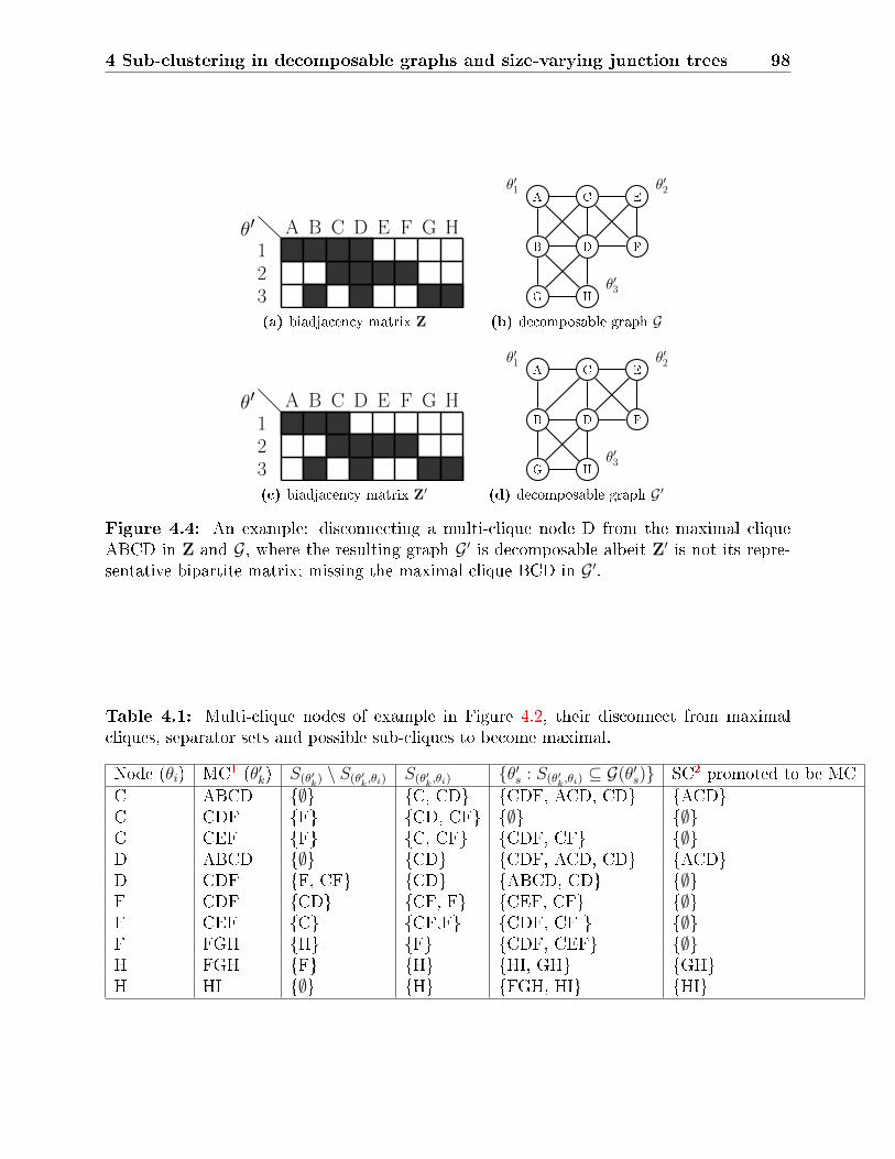
4 Sub-clustering in decomposable graphs and size-varying junction trees 98

θ′123

A B C D E F G H

(a) biadjacency matrix Z

B

A C

D

E

F

G H

θ′1 θ′2

θ′3

(b) decomposable graph G

θ′123

A B C D E F G H

(c) biadjacency matrix Z′

B

A C

D

E

F

G H

θ′1 θ′2

θ′3

(d) decomposable graph G′

Figure 4.4: An example: disconnecting a multi-clique node D from the maximal cliqueABCD in Z and G, where the resulting graph G ′ is decomposable albeit Z′ is not its repre-sentative bipartite matrix; missing the maximal clique BCD in G ′.

Table 4.1: Multi-clique nodes of example in Figure 4.2, their disconnect from maximalcliques, separator sets and possible sub-cliques to become maximal.

Node (θi) MC1 (θ′k) S(θ′k)\ S(θ′k,θi)

S(θ′k,θi)θ′s : S(θ′k,θi)

⊆ G(θ′s) SC2 promoted to be MC

C ABCD ∅ C, CD CDF, ACD, CD ACDC CDF F CD, CF ∅ ∅C CEF F C, CF CDF, CF ∅D ABCD ∅ CD CDF, ACD, CD ACDD CDF F, CF CD ABCD, CD ∅F CDF CD CF, F CEF, CF ∅F CEF C CF,F CDF, CF ∅F FGH H F CDF, CEF ∅H FGH F H HI, GH GHH HI ∅ H FGH, HI HI

4 Sub-clustering in decomposable graphs and size-varying junction trees 99

A

B C

D

E

F

G

H

I

(a) disconnecting C from ABCD toform ACD

ABCD CDF

AB

CF

CDA

ACDBD

AC ABD CDF

ACD

AC

AB CF

CDA

BD

(b) corresponding new junction tree

A

B C

D

E

F

G

H

I

(c) disconnecting H from FGH to formFG

CEF FGH

HI

GH

EF

CF

HI

CEF FG

HI

EF

CF

HI

(d) corresponding new junction tree

Figure 4.5: Examples of disconnecting multi-clique nodes of the example in Figure 4.2.The graph in the top panel (top left) shows the example of disconnecting C from ABCD,cases (i.c) and (ii.a) of Proposition 6, where the separator CD belongs to the sub-cliqueACD, making it maximal. The junction tree (top right) is rewired accordingly, and nosub-clique is discarded. The graph in the bottom panel (bottom left) illustrates the case ofdisconnecting H from FGH to form FG, while discarding the sub-clique GH, as in (i.a) and(ii.a) of Proposition 6, since FG∩HI is empty, the junction tree (bottom right) is rewiredaccordingly.

4.3.3 Connecting nodes

The last piece of the puzzle is the node connection move. Recall in (3.11), nodes connect

to maximal cliques that are adjacent, in some junction tree, to cliques already with the

node's connection. Section 3.3 assumed that a junction tree is known, while that did not

guarantee the full connectivity of a sampled graph, it ensured an underlining tree structure

which can partly, if not entirely, be discerned from the sampled graph. Nonetheless, as we

sample junction trees simultaneously with the graph, in certain cases, multiple disconnected

junction trees and single-node cliques can exist, as shown in Subgure 4.5c. While this

does not demand broad changes to the previously allowed connect moves, it calls for more

1maximal clique2sub-clique

4 Sub-clustering in decomposable graphs and size-varying junction trees 100

bookkeeping, which is illustrated by the following proposition.

Proposition 7. Let G be a decomposable graph, where G consists of two disjoint components

(Gt)t=1,2, such that no element in G1 is connected to an element of G2. Suppose that θ′s is a

non-empty clique in G1, and θi is a node of G that is not connected to any element of θ′s. If

any of the following holds:

(i) θi ⊂ G2;

(ii) θ′s is maximal in G1 and adjacent to θ′k in some junction tree, where θi ⊂ G(θ′k);

(iii) θ′s is a sub-clique in a maximal clique θ′m that is adjacent to θ′k in some junction tree,

where θi ⊂ G(θ′k) and G(θ′m) ∩ G(θ′k) ⊂ G(θ′s).

Then, the graph G ′ formed by connecting θi to every element of θ′s is decomposable.

Proof. For cases (i) and (ii) the proof of decomposability is direct by applying Theorem 11,

where in (i) a junction tree is formed by combining junction trees of both disjoint parts.

In (ii) since θ′k, θ′s ∈ E for some junction tree T = (C, E), adding θi to θ′s does not alter

any separator, and thus a junction tree exits. For (iii), since θ′k, θ′s ∈ E for some junction

tree T = (C, E) and G(θ′m) ∩ G(θ′k) ⊂ G(θ′s), then separators of each maximal clique are

intact, while θ′s ∪ θi becomes maximal and enters the tree in the middle of both maximal

cliques.

The following corollary builds on Proposition 7 by listing junction tree eects for each

move type.

Corollary 5 (Connecting nodes). Following the settings in Proposition 7, for some junction

tree T = (C, E) of G, suppose θi ∈ θ′k and θi ∈ θ′s, for some cliques θ′k, θ

′s, then

(i) when θi and θ′s of two disjoint components of G and θ′s is a sub-clique of θ′m ∈ C,

connecting θi to every element of θ′s results in a decomposable graph G ′ with junction

tree

T ′ =(C ∪ θ′s, E ∪

θ′k, θ′s, θ′m, θ′s

)

4 Sub-clustering in decomposable graphs and size-varying junction trees 101

where θ′k is not a single-node clique, otherwise T ′ = (C ∪ θ′s, E ∪θ′m, θ′s

. If θ′s is

maximal, then T ′ =(C, E ∪

θ′k, θ′s

)when θ′k is not a single-node clique, otherwise

T ′ = T .

(ii) when θ′s is maximal and θ′k, θ′s ∈ E, if θ′s diers from θ′k by only θi, then connecting

θi to every element of θ′s results in a junction tree T ′ = (C ′, E ′) with

C ′ = C \ θ′k, E ′ =E \θ′k, θ′m : θ′k, θ′m ∈ E

⋃θ′s, θ′m : θ′k, θ′m ∈ E

,

otherwise T ′ = T .

(iii) when θ′s is a sub-clique of some maximal clique θ′m ∈ C, such that θ′k, θ′m ∈ E, and if

G(θ′k) ∩ G(θ′m) ⊂ G(θ′s), then connecting θi to every element of θ′s results in a junction

tree T ′ = (C ′, E ′) with

C ′ = C ∪ θ′s, E ′ =E \θ′k, θ′m

⋃θ′k, θ′s, θ′s, θ′m

.

Remark. The connect move does not require any discarding or modifying of sub-cliques, since

in all the three cases of Proposition 7, other sub-cliques would retain their status.

Figure 4.6 illustrates an example of connecting a node to an adjacent sub-clique, such

that, (iii) from Corollary 5 applies.

4.4 Promoting a sub-clique to be maximal

Both disconnect moves, single-node and multi-node, are associated with a secondary post-

disconnection move that allows a sub-clique to be maximal, as in Denition 10. The choice

of which sub-clique to become maximal might be large. In essence, the only probabilistic

quantities that could drive such a choice are the clique-node anity parameters. Section 3.3.1

characterized those parameters with a latent unit rate Poisson process (θ′k, ϑ′k) ∈ Π′ on

4 Sub-clustering in decomposable graphs and size-varying junction trees 102

A

B C

D

E

F

G

H

I

(a) connecting H to EF to form EFH

CEF FGH

HI

GH

EF

CF

HI

CEF FGH

HI

GH

EFH

CF

HI

(b) corresponding new junction tree

Figure 4.6: An example of connecting a node to a sub-clique in an adjacent maximalclique. Node H connects to the sub-clique EF (left) from the example in Figure 4.2, by (iii)of Corollary 5 this forms the new maximal clique EFH connecting maximal cliques CEF andFGH.

R2+, where (θ

′k) index the locations and (ϑ′

k) index the weights of those clique-nodes. Albeit,

at each update step, the contents and size of possible sub-cliques might dier to a large

extent. Nonetheless, by their intrinsic nature decomposable graphs favour large connected

components, such as the maximal cliques. To mimic this tendency while avoiding the heavy

work of accounting for all combinatorially possible sub-cliques, we therefore take advantage

of the continuity of the anity parameters by promoting the sub-clique with the largest

weight.

Denition 11 (Promoting a sub-clique to be maximal). Fallowing the settings of Proposi-

tions 4 and 6, let θi be a node of a maximal clique θ′k ∈ C in a decomposable graph G. Let

S(θ′k,θ′i)be the set of separators of θ′k containing θi, such that

S(θ′k,θ′i)= θ′k ∩ θ′s : θi ∈ θ′s ∈ C.

Let C(θ′k,θi)be the set of sub-cliques, index by their weights, of θ′k that could be maximal if

θi disconnects from θ′k, as

C(θ′k,θi)=ϑ′m : (θ′m, ϑ

′m) ∈ Π′, θi ∈ θ′m, S(θ′k,θi)

⊂ θ′m ⊂ θ′k.

Then, if C(θ′k,θi)= ∅, (θ′o(k,i), ϑ′

o(k,i)) is promoted to be maximal if the disconnection occurs,

4 Sub-clustering in decomposable graphs and size-varying junction trees 103

where

o(k, i) =s ∈ N : ϑ′

s = max(C(θ′k,θi)

),

the index of the largest element in C(θ′k,θi)with respect to the natural ordering in R+.

Denition 11 elaborates on 10, and thus applies to Corollary 4 and Proposition 6 (i.c), of

disconnect moves. In the connect move of Corollary 5, a sub-clique could become maximal;

however, it is a direct result of the connect move and not a secondary move. In this case, no

promotion occurs.

Denition 11 pins down the choice of which sub-clique to become maximal after a discon-

nection to one choice, if any. This streamlines the Markov update steps, from three steps: a

disconnect move, a secondary sub-clique promotion move, and a junction tree update move,

to two steps by eliminating the secondary sub-clique move. The next section summarizes all

update steps in a concise iterative Markov update scheme.

4.5 Markov updates under size-varying junction trees

Following the notations of (3.6), (3.7) and (3.8), for a decomposable graph G with some

junction tree T = (C, E), dene the θi-induced junction tree at the n-th update step, T (n)|i,

as in (3.6). Expand the denition of boundary clique-nodes of (3.7) to include maximal

cliques with multi-clique separator sets and sub-cliques. Moreover, expand the denition of

neighbouring clique-nodes of (3.7) to include sub-cliques of maximal cliques in T (n)|i and

sub-cliques of neighbouring cliques that retain the set intersection nodes, as follows:

T(n)|ibd =

θ′s : θ

′i ∈ θ′s,

(θ′s ∈ C ∧ S(θ′s,θi) ⊆ θ′k s.t. s = k

)∨(θ′s ∈ C

),

T(n)|inei =

θ′s : θi ∈ θ′s,∃θ′k ∈ T (n)|is.t.

(θ′k, θ′s ∈ E

)∨(θ′s ⊂ θ′m ∧ θ′m ∩ θ′k ⊂ θ′k ∧ θ′k, θ′m ∈ E

)∨(θ′s ⊂ θ′k

).

(4.2)

Dene the n+1 Markov iterative update step for the bipartite matrix Z with sub-cliques

4 Sub-clustering in decomposable graphs and size-varying junction trees 104

and size-varying junction tree as:

(i) update the edge z(n+1)ki given the current conguration Z(n) as:

P(z(n+1)ki = 1 | Z(n), T ) = W (n+1)(ϑ′

k, ϑi) =

⎧⎪⎪⎨⎪⎪⎩W (ϑ′

k, ϑi) if θ′k ∈ T(n)|ibd

⋃T

(n)|inei ,

z(n)ki otherwise.

(4.3)

(ii) given the new edge z(n+1)ki update the junction tree T as

• for a connect move: update T according to Corollary 5;

• for a disconnect move, using Denition 11:

if θ′k is a single-clique node, update T as in Proposition 4 and Corollary 4 ;

if θ′k is a multi-clique node, update T as in Proposition 6.

The Markov update steps can be iterated until convergence.

4.6 Discussion

This chapter has introduced a method to model sub-clusters within decomposable graphs.

This is done by extending the biadjacency representation to allow for interactions between

graph nodes and subgraphs of maximal cliques. Subgraphs of maximal cliques, or as termed

sub-maximal cliques, can naturally be seen as sub-clusters within each maximal clique. The

ability of the biadjacency representation to account for such sub-cliques adds richness to

this representation and opens doors for new applications of decomposable graphs. Rather

than solely modelling decomposable graphs, as in the classical settings, it is now possible to

model both the decomposable graph and the latent dynamics forming within each maximal

clique. Such dynamics are generally seen in behavioural type of data, such as behaviour

economics or politics. For example, maximal cliques can represent rms or political entities,

where interactions ow through specic channels. Sub-clustering dynamics can then capture

4 Sub-clustering in decomposable graphs and size-varying junction trees 105

interactions within each entity or larger maximal clique. An interesting dynamic captured

by this model, is when larger entities conglomerate in even larger maximal cliques, or when

sub-cliques separate to form independent entities.

The exibility and depth that are gained by allowing for sub-clustering in the biadjacency

matrix comes with extra complexities, primarily related to the dynamics between maximal

and sub-maximal cliques. It is not clear how these dynamics should be structured, for

example; when disconnecting a node from a maximal clique, does it also disconnect from

all sub-maximal cliques of the former? This chapter adopts the notion that a node would

not disconnect from a sub-maximal clique when disconnecting from a maximal. Instead, in

the junction tree update move, using the continuity of anity parameters, the sub-maximal

clique with the highest anity parameter would be labelled as maximal, if possible, and

added to the junction tree. The node would then disconnect from all other sub-maximal

cliques that became improper with this disconnection. In the connect move, the update

rules are less complex. Contrary to the treatment of decomposable graphs in Chapter 3,

allowing for sub-clustering requires a series of rules addressing the change in the junction

tree after every (dis)connect move. In some update steps, a maximal clique might become

sub-maximal and the opposite, varying the size of the junction tree at every step. A major

part of this chapter is dedicated to such update rules.

The clustering mechanism proposed in this section does not depend on choosing the

correct number of clusters, nor on choosing a proper clustering distance. As discussed in

Section 3.3, an n-node graph can have a maximum of n maximal cliques, with n isolated

nodes, and a minimum of 1, with a fully connected graph. This chapter adopted a xed size

biadjacency matrix Z; therefore, as long as the number of rows is larger than the number of

columns, one can potentially infer the correct number of maximal cliques. All other latent

communities would be labelled as sub-clusters.

One possible improvement for this work is a method for deciding how many sub-clusters

are desired. Do we use a square biadjacency matrix Z, or double the number of rows to

4 Sub-clustering in decomposable graphs and size-varying junction trees 106

columns? A possible solution would be to use a very large number of rows, and then skim

all small sub-clusters, for example, single-node sub-clusters. A possible direction for future

work is to adopt a sub-clustering framework that is in between the proposed method of this

chapter and the initial treatment of decomposable graphs of Chapter 3. Tree nodes θ′1, θ′2, . . .

were initially treated as the maximal cliques of a decomposable graph, such that the Markov

update step of (3.12) used the boundary and neighbouring sets of (3.8). This guarantees

that all active cliques are maximal. Nonetheless, as shown in Proposition 1, using the

boundary and neighbouring sets of (3.7) also guarantees that the mapping in (3.10) results

in a decomposable graph; though, not all active cliques in the biadjacency representation are

maximal. This also amounts to another direction of sub-clustering in decomposable graphs,

where the sub-clusters are the non-empty non-maximal nodes of the tree. This method

could potentially lead to less complex update steps, though the interpretation of sub-clusters

diers from the one proposed in this chapter. The dierence is that sub-maximal cliques are

potentially maximal as more nodes are added to the model, and thus are only temporary

sub-clusters.

107

Chapter 5

A Bayesian model for link prediction in

ecological networks

Identifying undocumented or potential interactions among species is a challenge facing mod-

ern ecologists. Our aim is to guide the sampling of ecological networks by identifying the

most likely undocumented interactions. We frame this problem using a bipartite graph

structure, where edges represent interactions between pairs of species. We rst construct a

prior network of associations by drawing from available literature. To predict undocumented

interactions, we use a hierarchical Bayesian latent score framework for bipartite graphs and

incorporate a Markov network dependence informed by phylogenetic relationships among

species. The addition of phylogenetic information to the model has a signicant improvement

in predictive accuracy. We show that such a model can easily incorporate count or binary

data, and dierent forms of neighbourhood structure. We demonstrate this model using two

host-parasite networks constructed from published databases, the Global Mammal Parasite

Database and the Enhanced Infectious Diseases database, each with thousands of pairwise

interactions. We additionally extend the model by integrating a correction mechanism for

missing interactions in the observed data, which proves valuable in reducing uncertainty in

unobserved interactions.

5 A Bayesian model for link prediction in ecological networks 108

5.1 Introduction

Ecological interactions impact the structure of populations and communities, drive co-

evolution, and can determine the functioning of ecosystems (Heleno et al., 2014). Analysis

of species interaction networks can be used to better understand the generation and stability

of ecosystems, and to identify communities and species that are vulnerable to environmental

change (Araújo et al., 2011; Ings et al., 2009). However, most ecological networks are only

partially observed and fully characterizing all interactions via systematic sampling involves

substantial eort and investment that is not feasible in most situations (Jordano, 2015).

The interest in inferring undocumented interactions and projecting interactions into the fu-

ture have made predicting species interactions a major challenge in ecology (Kissling and

Schleuning, 2015; Morales-Castilla et al., 2015). One approach to eectively ll-in gaps in

interaction networks would be targeted sampling based on verifying highly probable, yet

previously undocumented links.

In this chapter, we propose a new framework for predicting ecological interactions, and

evaluate it using two host-parasite networks. This approach departs from what has been

considered in the literature to date in three main ways. First, we describe a hierarchical

Bayesian latent variable framework for link prediction based on generative models of bipar-

tite graphs. The latent variable acts as an underlying scoring system, with higher scores

attributed to more probable links. This framework is motivated by recent work in recom-

mender systems, such as Ekstrand et al. (2011), Breese et al. (1998), which oer generalized

methods for identifying novel interactions in partially observed bipartite networks. For a

thorough review of recommender systems, see Ricci et al. (2011).

Second, we incorporate a exible Markov network dependence among nodes that we

encode using phylogenetic information in the form of a species similarity matrix. Phylogeny

is a representation of the evolutionary relationships among species, which provides a means

to quantify ecological similarity (Wiens et al., 2010). Just as many species traits co-vary with

phylogeny, species interactions are also phylogenetically structured in both antagonistic (ex.

5 A Bayesian model for link prediction in ecological networks 109

herbivory, parasitism) and mutualistic (ex. pollination, seed dispersal) networks (Gómez

et al., 2010). Encoding the Markov network as a similarity matrix allows for straightforward

expansion to dierent forms of dependence if phylogenetic information is unavailable, or

other dependence structures are preferred.

Third, we integrate a mechanism that accounts for uncertainty in undocumented inter-

actions, and proves valuable in reducing the overlap in posterior probability densities for

interacting and non-interacting pairs. A limitation of observational data is the nature of

unobserved interactions as most data sources provide information only for documented in-

teractions (Morales-Castilla et al., 2015). Thus, the absence of a documented interaction

cannot be taken as evidence that a species pair would not interact given sucient opportu-

nity.

We demonstrate this model by predicting undocumented interactions in subsets of two

published host-parasite databases. Each database consists of thousands of documented inter-

actions based on evidence presented in peer-reviewed articles or mined from genetic sequence

metadata.

5.2 Bayesian hierarchical model for prediction of ecolog-

ical interactions

5.2.1 Network-based latent score model

Given an interaction matrix for two sets of species, for example H hosts and J parasites, of

which we only observe a portion of the possible interactions, our interest is to predict missing

interactions and rank them starting with the most likely ones. Let the binary variable zhj

denote whether an interaction between host h and parasite j has been observed, such that

zhj = 1 if its established that host h carries parasite j, zhj = 0 otherwise, for h = 1, . . . , H

and j = 1, . . . , J . Moreover, assume a continuous anity (popularity) parameter for each

5 A Bayesian model for link prediction in ecological networks 110

host and each parasite based on its observed number of interactions in the network. This

parameter governs the general propensity for each organism to interact with members of

the other class. The larger the value of the anity parameter the more likely an organism

to interact: for example, a host would be susceptible to a larger number of parasites, or a

parasite would infect a larger number of hosts. Let γh > 0 be the anity parameter of host

h , and ρj > 0 for parasite j. Using a log-multiplicative form we dene the anity-only

model by setting the conditional probability of interaction to

P(zhj = 1 | Z−(hj)) = 1− exp(−γhρj), (5.1)

where Z−(hj) is the matrix Z excluding zhj.

The anity-only model can result in a workable network prediction model, as been shown

in the literature on exchangeable random networks in Bickel and Chen (2009); Chung and Lu

(2006); Ho et al. (2002), and others. However, the log-linear form in (5.1) tends to generate

an adjacency matrix with many hyperactive columns and rows. This is due to the fact that

whenever a node has a suciently high anity parameter it forms edges with almost all other

nodes, which may be unrealistic for most ecological networks. To improve the anity-only

model, we add a Markov network dependency that is based on a normalized host similarity

matrix informed by host phylogeny. Let ∆ be an H ×H matrix that quanties the pairwise

similarity between hosts, where higher values imply stronger correlations. ∆ is normalized

such that 0 < ∆hi < 1 for all h, i ∈ 1, . . . , H, h = i. Thus, we dene the full model to be

P(zhj = 1 | Z−(hj)) = 1− exp(−γhρjδηhj), δηhj =H∑i=1i =h

∆ηhizhj. (5.2)

The intuition behind this construction is that a host h is more likely to connect to a

parasite j if there are many hosts that are similar to h and at the same time connected with

j. This is done by summing the scaled similarities between h and those hosts having an edge

5 A Bayesian model for link prediction in ecological networks 111

connection with j in δηhj, increasing the probability for high values of δηhj, and penalizing it

for low values.

The scaling coecient η adjusts the trade-o between rewarding and penalizing the in-

teraction probabilities, where large values of η pressure δηhj to take more of a penalizing role,

while small values allow more rewards. Nonetheless, very small values of η suggest a weaker

explanatory power of the used similarity measure (∆), since δηhj →∑H

i=1,i =h zhj as η → 0,

which are simply the column sums driving the parasite anity parameter ρj. In other words,

for very small values of η, the model in (5.2) converges to an anity-only model under a

dierent parametrization.

We remark that the full model in (5.2) could also be seen as a layering of two models,

where the rst is a bipartite anity-only network model represented in (5.1), and the second

is the phylogeny-only model, that is

P(zhj = 1 | Z−(hj)) = 1− exp(−δηhj), (5.3)

where δηhj as in (5.2)

Later, in Section 5.4.3, we show that both models, the anity-only and phylogeny-

only, independently result in suitable predictive models that are adequate to represent some

variation in the data. However, each model captures dierent characteristics of the graph

and layering them, as in (5.2), we obtain a non-trivial improvement. This is primarily due

to the anity-only model (5.1) resulting in a highly dense posterior interaction matrix, and

penalizing by the phylogeny-only model (5.3) helps in reducing this phenomena.

Driven by recent work in network modelling, such as in Ho et al. (2002) and Ho (2005),

we nd it advantageous to use latent variables in modelling the binary variables zhj. This

facilitates the construction of the network joint distribution in this model, and it eases the

integration of a Markov network dependence that accounts for similarities among hosts. The

latter is crucial to address the ambiguity associated with the case when zhj = 0, which entails

5 A Bayesian model for link prediction in ecological networks 112

two possibilities: a yet to be observed positive interaction, or a true absence of interaction

due to incompatibility. Thus, for each zhj we dene a latent score shj ∈ R such that

zhj =

⎧⎪⎪⎨⎪⎪⎩1 if shj > 0

0 otherwise.

(5.4)

The values of the latent scores, although unobserved, completely determine the binary

variables zhj. The conditional model in (5.2) can be completely specied in terms of the

latent score as

P(zhj = 1 | Z−(hj)) = E[Ishj>0 | Z−(hj)] = P(shj > 0 | S−(hj)) (5.5)

where IA is the indicator function, resulting in 1 if A occurs, otherwise 0, and S−(hj) represents

the interaction matrix S excluding shj, replacing Z as it carries the same probability events.

Given the construction above, we use a zero-inated Gumbel distribution for the latent

score with the following density

p(shj | S−(hj)) = τhj exp(−shj − τhje−shj)Ishj>0 + exp(−τhj)Ishj=0, (5.6)

where τhj = γhρjδηhj. Hence, the conditional joint distribution becomes

P(zhj = 1, shj | Z−(hj)) = P(zhj = 1 | shj)p(shj | S−(hj)) = p(shj | S−(hj))Ishj>0 (5.7)

The construction used in this section reduces the number of parameters to estimate from

H × J to H + J + 1 by taking advantage of the bipartite graph structure.

5 A Bayesian model for link prediction in ecological networks 113

5.2.2 Prior and Posterior distribution of choice parameters

The choice of a zero-inated Gumbel was made to facilitate the construction of the joint

distribution, in a manner similar to the Swendsen-Wang algorithm (Swendsen and Wang,

1987), where the product of densities transform to a sum in the exponential scale. Alterna-

tively, a similar parametrization can be achieved using a truncated exponential distribution,

as shown in Appendix A.1.1, though it does not admit the direct interpretability as a latent

score as with the Gumbel distribution.

Let shj be distributed as in (5.6), such that zhj is completely determined by shj. By a

conditional construction the latent score joint distribution is

P(S,Z |,γ,ρ, η) =J∏

j=1

[P(S.j ,Z.j |γ,ρ, η)

]

=

J∏j=1

H∏h=1

[(γhρj δ

ηhj exp (−shj − γhρj δ

ηhje

−shj )

)zhj(e−γhρj δ

ηhj

)1−zhj]

=

[ J∏j=1

ρmj

j

][ H∏h=1

γnh

h

][ J,H∏h,j

(δηhj)zhj

]exp

(−

J,H∑h,j

shjzhj + ρjγhδηhje

−shjzhj

),

(5.8)

where .j represent the j-th column of S.j and Z.j, mj =∑H

h=1 zhj, nh =∑J

j=1 zhj, and

δηhj =∑h−1

i=1 ∆hizij = δηhj −∑H

i=h+1 ∆hizij = δηhj − δηhj, with the convention that δη1j = 1,

as the initial parasite infection is assumed to follow a dierent design. Moreover, by con-

structing the joint distribution from conditioning, the order of observation does inuence

the joint distribution, as seen by the δηhj component. This dependence is omitted but im-

plicitly assumed, nonetheless, the joint distribution is still valid by conditioning on a xed

order. Using the Hammersley-Cliord theorem (Robert and Casella, 2013), one can prove

the existence of a full joint distribution, and that this joint distribution is not aected by

ordering of observations, see Appendix A.1. Though, (5.8) allows one to derive the full joint

distribution of any order.

As a result of the embedded Markov random eld structure in δηhs, it is harder to work

with the marginal distribution P(Z | γ,ρ, η), since it has to be specied conditionally.

5 A Bayesian model for link prediction in ecological networks 114

Therefore, we build the joint posterior distribution in terms of latent score as

P(S,γ,ρ, η | Z) ∝ P(Z | S)P(S | γ,ρ, η)P(γ)P(ρ)P(η), (5.9)

For the prior specications, we choose a gamma distribution for both γ and ρ for their

conjugacy property, thus let γhiid∼ Gamma(αγ, τγ) and ρj

iid∼ Gamma(αρ, τρ), the conditional

posterior distributions of γh and ρj, respectively, are

ρj | S,γ, η,Z ∼ Gamma

(αρ +mj, τρ +

H∑h=1

γhδηhje

−shj

),

γh | S,ρ, η,Z ∼ Gamma

(αγ + nh, τγ +

J∑j=1

ρj δηhje

−shj

).

(5.10)

Many ecological and other real world networks display power-law degree distributions

(Albert and Barabasi, 2002). This is also the case with the host-parasite databases used in

this chapter, where both margins, hosts and parasites, exhibit power-law degree distributions

(see Appendix Figure 5.2). The anity only model (5.1) has been shown to generate a

power-law behaviour when a Generalized Gamma process is used (Brix, 1999; Caron and

Fox, 2014; Lijoi et al., 2007). In fact, when γh = γ for all h, the anity-only model behaves

much like the Stable Indian Buet process of Teh and Gorur (2009) that has a power-

law behaviour. Nonetheless, the full model of (5.2) does show a signicant improvement in

predictive accuracy over the anity-only model, though it does not yield a degree distribution

with a power-law.

In the case of the scaling parameter η, for simplicity and computational stability, we as-

sume an at non-informative prior as uniform[0,100], although this could be readily modied

to be any required subjective prior.

5 A Bayesian model for link prediction in ecological networks 115

Finally, the latent score is updated, given all other parameters as

shj | Z,ρ,γ, η ∼

⎧⎪⎪⎨⎪⎪⎩χ0 if zhj = 0

tGumbel

(log(γhρjδ

ηhj), 1, 0

)if zhj = 1,

(5.11)

where χ0 is an atomic measure at zero and tGumbel(τ, 1, 0

)is the zero-truncated Gumbel,

having the density

exp(−(s− τ + e−(s−τ)))

1− exp(−eτ ) χ(0,∞)(s).

5.2.3 Markov Chain Monte Carlo algorithm

By introducing a Markov network dependence among hosts using the variable δηhj, the

marginal posterior predictive distribution of each interaction zhj can only be constructed

conditionally on all other interactions, Z−(hj), as shown in (5.2). To preserve the MCMC

convergence conditions, one should update all parameters after sampling each latent score

shj in a sweeping manner. Thus, to get a single sample of an H × J matrix S one needs to

sample all parameters H × J times. To speed up computations we apply a block sampler.

First, note that each latent score shj depends only on row h and column j via the parameters

γh and ρj, and on η via the dependence variable δηhj. Hence, for H ≤ J , one can update

all anity parameters related to the elements of the diagonal block shh : h = 1, . . . , H in

parallel while retaining convergence conditions. This reduces the sampling of a single S to

J MCMC cycles, where the elements of each diagonal block

sh,(h+i) mod J : h = 1, . . . , H

are sampled in parallel for i = 0, . . . , J−1. For example, the parameters of the i-th diagonal

block are γ1, . . . , γH and ρ(h+i mod J), . . . ρ(2h+i mod J). Using this diagonal update scheme, each

parameter is then sampled in turn conditional on all the rest. Both, γ and ρ are sampled

5 A Bayesian model for link prediction in ecological networks 116

using direct sampling from the posterior in (5.10). The scale parameter η is sampled using

an Adaptive Metropolis-Hastings algorithm (Haario et al., 2001), where a new proposal η is

sampled from a log-normal distribution as q(η | η) = lognormal(log(η), σ2η) given a at prior,

and the proposal acceptance probability is

min

1,

[ H,J∏h,j

(δηhjδηhj

)zhj]exp

(−

H,J∑h,j

γhρjeshj(δηhj − δηhj

)). (5.12)

Iteratively, after updating the model parameters, we use an Adaptive Metropolis-Hastings

algorithm to also update the hyperparameters (αγ, τγ, αρ, τρ), for more details refer to Ap-

pendix B.

So far, we have assumed that the information given in Z is denite, that the observed

links are presences and unobserved ones are absences. However, as discussed previously, we

believe this will not be the case for many ecological networks. The next section introduces

a method in dealing with such cases.

5.3 Uncertainty in unobserved interactions

In ecological networks it is unlikely that all potential links among species will occur. Some

unobserved links exist but are undocumented due to limited or biased sampling, while others

may be true absences or "forbidden" links (Morales-Castilla et al., 2015). Evidence used to

support an interaction will vary depending on the nature of the system, but it often assumes

that an interaction exists if at least one piece of evidence indicates so (Jordano, 2015).

This kind of construction raises concern about the uncertainty of interactions in two ways.

The rst concern is due to uncertainty in documented interactions as false positive detection

errors may occur, potentially as a result of species misidentication, sample contamination,

or unanticipated cross-reactions in serological tests. We believe it would be useful for the

scientic community to identify weakly supported interactions that may require additional

supporting evidence, however our primary motivation is identication of "novel" interactions,

5 A Bayesian model for link prediction in ecological networks 117

which is complicated by uncertainty in unobserved interactions.

The second concern arises when unobserved associations are by default assumed to be

negative. As discussed earlier, ecological networks are often under-sampled, and some frac-

tion of unobserved interactions may occur but are currently undocumented, or represent

potential interactions that are likely to occur given sucient contact. Based on this assump-

tion we build a measure of uncertainty in unobserved interactions by modifying the proposed

model. In (5.4), we have assumed that zhj is a deterministic quantity given shj | Z−(hj), and

thus we have only sampled positive scores for the case when zhj = 1, as shown in (5.11). As a

result, in the prediction stage, the posterior predictive distribution in (5.2) is only considered

for the case when a pair has no documented associations (zhj = 0), and it is deterministic

with probability 1 otherwise, underlining the assumption that the dataset is complete and

trusted. In reality, this assumption does not hold. Thus to account for uncertainty in unob-

served associations, we attempt to measure the percentage of positive scores for where the

input is 0 (zhj = 0), as

p(zhj = 0 | shj, g) =

⎧⎪⎪⎨⎪⎪⎩1, if shj = 0,

g, if shj > 0.

(5.13)

In a sense, the construction above attempts to measure the proportion of missing links

in the observed data, where g is the probability that an interaction is unobserved when the

latent score indicates an interaction should exist. If g is large and close to 1, it is likely

that many of the unobserved interactions are likely to exist. Introducing g to the model

aects all parameter estimates and the notion of Z, therefore, in the post prediction stage,

the posterior predictive distribution is now considered for both cases. For the case of a

documented association, the probability of an interaction is dened in (5.2), and for the

case of no documentation the same probability is weighted by g as shown in more details in

(5.14).

5 A Bayesian model for link prediction in ecological networks 118

This kind of construction has been used earlier by Weir and Pettitt (2000) when modelling

spatial distributions to account for uncertainty in regions with unobserved statistics, and

later by Jiang et al. (2011) in modelling uncertainty in protein functions.

5.3.1 Markov Chain Monte Carlo algorithm

Introducing a measure of uncertainty in the model does not alter the MCMC sampling

schemes introduced in Section 5.2.3. The variables γ,ρ and η are still only associated with

S, nonetheless, by introducing the measure of uncertainty, the conditional sampling of each

individual shj is now

p(shj | S−(hj),Z, g) =

⎧⎪⎪⎪⎪⎪⎪⎪⎪⎪⎪⎪⎨⎪⎪⎪⎪⎪⎪⎪⎪⎪⎪⎪⎩

1ψ(shj)

τhj exp

(−(shj + τhje

−shj )

), shj > 0, zhj = 1,

0, shj = 0, zhj = 1,

gθ(g,shj)

τhj exp

(−(shj + τhje

−shj )

), shj > 0, zhj = 0,

1θ(g,shj)

1− ψ(shj), shj = 0, zhj = 0,

(5.14)

where τhj = γhρjδηhj, ψ(shj) =

∫∞0

p(s | S−(hj))ds = 1 − exp

(−γhρjδηhj

), and θ(g, shj) =

gψ(shj) + 1− ψ(shj).

Moreover, sampling the uncertainty variable is performed using the conditional distribu-

tion as

P(g | S,Z) ∝ P(Z|S, g)P(S | g) P(g) ∝ gN−+(1− g)N++ , (5.15)

where N−+ = #(h, j) : zhj = 0, shj > 0, N++ = #(h, j) : zhj = 1, shj > 0, and P (g) is a

uniform.

5 A Bayesian model for link prediction in ecological networks 119

5.4 A case study with host-parasite networks

5.4.1 Data

We implement this model on two databases, the Global Mammal Parasite Database (GMPD),

available at mammalparasites.org and documented by Nunn and Altizer (2005), and the

Enhanced Infectious Diseases (EID2) database, available at zoonosis.ac.uk/EID2 and doc-

umented in McIntyre et al. (2013) and Wardeh et al. (2015). Both databases are periodically

updated and contain associations between hosts and their parasites based on thousands of

published reports and scientic studies. The assumed interactions are based on peer-reviewed

articles that present empirical observations of associations between host-parasite pairs using

a variety of evidence types (visual identication, serological tests, or detection of genetic

material from a parasite species in one or more host individuals). Associations are reported

along with their publication or genetic sequence reference. More than one reference might be

reported per association, and by aggregation we can determine the count of unique references

per interaction.

The GMPD gathers data on wild mammals and their parasites (including both micro and

macroparasites), which is separated into three primary databases based on host taxonomy:

Primates, Carnivora, and ungulates (terrestrial hooved mammals from Artiodactyla and

Perissodactyla). For analyses we used the ungulate and Carnivora subsets updated by Huang

et al. (2015) to include articles published up to 2010. Counts of unique evidence supporting

each association were constructed according to the number of citations for each host-parasite

pair.

The EID2 database contains a broader scope of organism interactions and includes addi-

tional host groups not represented by the GMPD, including domesticated animals. However,

the host groups in the GMPD are not as well represented in the EID2 database. According

to Wardeh et al. (2015), ≈ 64% of unique interactions listed in the GMPD are found in EID2

and ≈ 30% of those in EID2 are found in the GMPD. For analyses, we used a static version

5 A Bayesian model for link prediction in ecological networks 120

of the EID2 published by Wardeh et al. (2015). We subset the database to include only

mammal hosts and removed interactions involving Homo sapiens. Counts of unique evidence

supporting each association were constructed by summing the number of publications and

unique genetic sequences reported for each host-parasite pair.

The GMPD and EID2 databases as described above were used to construct the binary

presence-only matrix Z, where zhj = 1 for pairs with documented associations, otherwise

zhj = 0. We let the pairwise similarity matrix (∆) to be the mammal phylogeny of Fritz et al.

(2009) which was taken as the inverse of the phylogenetic dissimilarity matrix calculated by

the function cophenetic in the R package ape (Paradis et al., 2004). Incorporating the

phylogeny required host names to be standardized to the taxonomy of Wilson and Reeder

(2005) which involved collapsing subspecies. In addition, we removed parasites reported only

to Genus level. This resulted in a GMPD subset with 3966 pairs of interactions among 246

hosts and 743 parasites, and an EID2 subset with 3730 pairs of interactions among 694 hosts

and 783 parasites. We nd both subsets suciently large to yield proper numerical results.

parasites

host

s

5 45 90 140 195 250 305 360 415 470 525 580 635 690

250

220

200

180

160

140

120

100

8060

4020

(a) GMPD

parasites

host

s

5 45 90 145 205 265 325 385 445 505 565 625 685 745

700

640

580

520

460

400

340

280

220

160

100

50

(b) EID2

Figure 5.1: Left ordered interaction matrix Z of GMPD (left) and EID2 (right) databases.

5 A Bayesian model for link prediction in ecological networks 121

Figure 5.1 shows the left-ordered interaction matrix Z of GMPD on the left, and the EID2

on the right. Both matrices are more or less of equal size. The EID2 has a few hosts that

interact with a large number of parasites, as seen by the horizontal strips, while the GMPD

shows a more even distribution across rows. Nonetheless, both matrices are quite sparse, and

the degree distributions of both hosts and parasites exhibit a power-law structure, as shown

in Figure 5.2. The degree distribution of parasites (blue stars) for the GMPD interaction

network shows steeper slope compared to the hosts degree distribution (red crosses). On

the other hand, the degree distribution of both hosts and parasites seem to have comparable

slopes in the EID2 interaction network.

*

*

*

*

*

**

*

**

*

*

* *

*

*

**

**

****

**

******

1 2 5 10 20 50 100

12

510

2050

100

200

500

Degree

Num

ber

of N

odes

+

+

+ +

+

+

++

+

+

+

+

+

+

+++

++

++

++

+

++

+

+

+

++

+

+

+

+

+

+

+

++

++++++

+

++

+

++++++++++++

*+

ParasitesHosts

(a) GMPD

*

*

*

*

*

**

*

*

* * *

* *

*

**

*

*

*

********

*

**

1 2 5 10 20 50

12

510

2050

100

200

500

Degree

Num

ber

of N

odes

+

+

+

+

+ +

++

++

++

+

++

++++

++

+

+

+

+

+

+++++++++++++

*+

ParasitesHosts

(b) EID2

Figure 5.2: Degree distribution of hosts (red crosses) and parasites (blue stars) on log-scale,for the GMPD (left) and EID2 (right) databases.

5.4.2 Parameter estimation

Using the GMPD and EID2 databases we rst t the model proposed in Section 5.2.1. We

run 12000 MCMC iterations for posterior estimates with 4000 burn-in. In total we have

J + H + 1 parameters to estimate: an anity parameter for each host and each parasite,

5 A Bayesian model for link prediction in ecological networks 122

and a scaling parameter for the similarity matrix. As well, for each database, we iteratively

sample the set of anity hyperparameters.

Standard convergence diagnostics showed that all parameters had converged. It is worth

noting that for the GMPD, the posterior distributions of the host parameters (γ) shows

large variations, which reects that some hosts are more likely to interact with parasites, or

have been more intensively studied. In the EID2 database, the variation among the hosts

is more prominent, which conrms our earlier observation that row densities of the EID2

interaction matrix are less balanced (see Figure 5.1 and Appendix Figure C.1). In both

databases, the magnitude of the scaling parameter η is signicantly greater than zero, which

indicates the importance of phylogeny in the dependence structure. For the GMPD η is

found to concentrate around 1.57, for the EID2 around 1.15. For additional convergence and

diagnostic plots, please refer to Appendix C.

5.4.3 Prediction comparison by cross-validation

To validate the predictive performance of the proposed latent score full model, we compare

it to three other variations and to a regular nearest-neighbour (NN) algorithm. So far, the

latent score full model in Section 5.2.1 is implemented using the presence-only matrix Z. We

vary this model in three ways, rst, we implement it without a dependence term, that is the

anity-only model as in (5.1). Second, we implement it with only the dependence term, that

is the phylogeny-only model in (5.3). Third, since the binary matrix Z ignores the count of

available evidence, which may be useful for increasing predictive performance in some cases,

we implement a weighted-by-counts version where the number of documented references for

each interaction are taken to be edge weights in constructing the similarity input variable δ

in (5.2). Such that

δηhj =H∑i=1

∆ηhi log(1 + yij),

5 A Bayesian model for link prediction in ecological networks 123

where yij is the documented association counts for the (i, j)-th host-parasite pair with yij = 0

if there are no documented associations.

Finally, we compare the latent score full model and the three variations to a regular NN

algorithm, in which we set the distances between hosts proportional to the number of parasite

species they share, namely ∆ = ZZ⊺ while enforcing the diagonal to zero. This particular

similarity matrix does not require additional data other than the observed interaction matrix

Z . This similarity matrix determine the host-neighbour structure and thus, conditional on

all the rest, we let the probability of a host-parasite interaction equal to the average number

of host-neighbours with documented association to the parasite, within the k-closest host-

neighbours. Consequently, we evaluate the model with dierent values for k and use the

value that results in the highest predictive accuracy.

Because the formulation of the host dependence structure requires parasites to have at

least one interaction, the hold out portion for cross-validation was restricted to parasites with

one or more associations in the data, and AUC values calculated using only this portion.

Therefore, the predictive performance of each model is evaluated by using the average of

5-fold cross-validations, where each fold sets approximately a random 17% of the observed

interactions (zhj = 1) in Z to unknowns (zhj = 0) while attempting to predict them using

the remaining portion. For the weighted-by-counts version we also set the corresponding

counts to 0 (yhj = 1). For each of the folds, we run a standard MCMC simulation to infer

the parameters of interest and to calculate the mean posterior probability of an interaction

for each of the unknowns. By uniformly thresholding those probabilities from 0 to 1, where

probabilities above the threshold are assumed to represent an interaction, we calculate the

true positive and negative rates, and the false positive and negative rates. By this process,

we nally obtain the receiver-operating characteristics (ROC) curves, and the posterior in-

teraction matrix resulting from the threshold that maximizes the area under the ROC curve

(AUC). Figure 5.3 illustrates the resulting ROC curves for the GMPD and EID2 databases,

under the tested models.

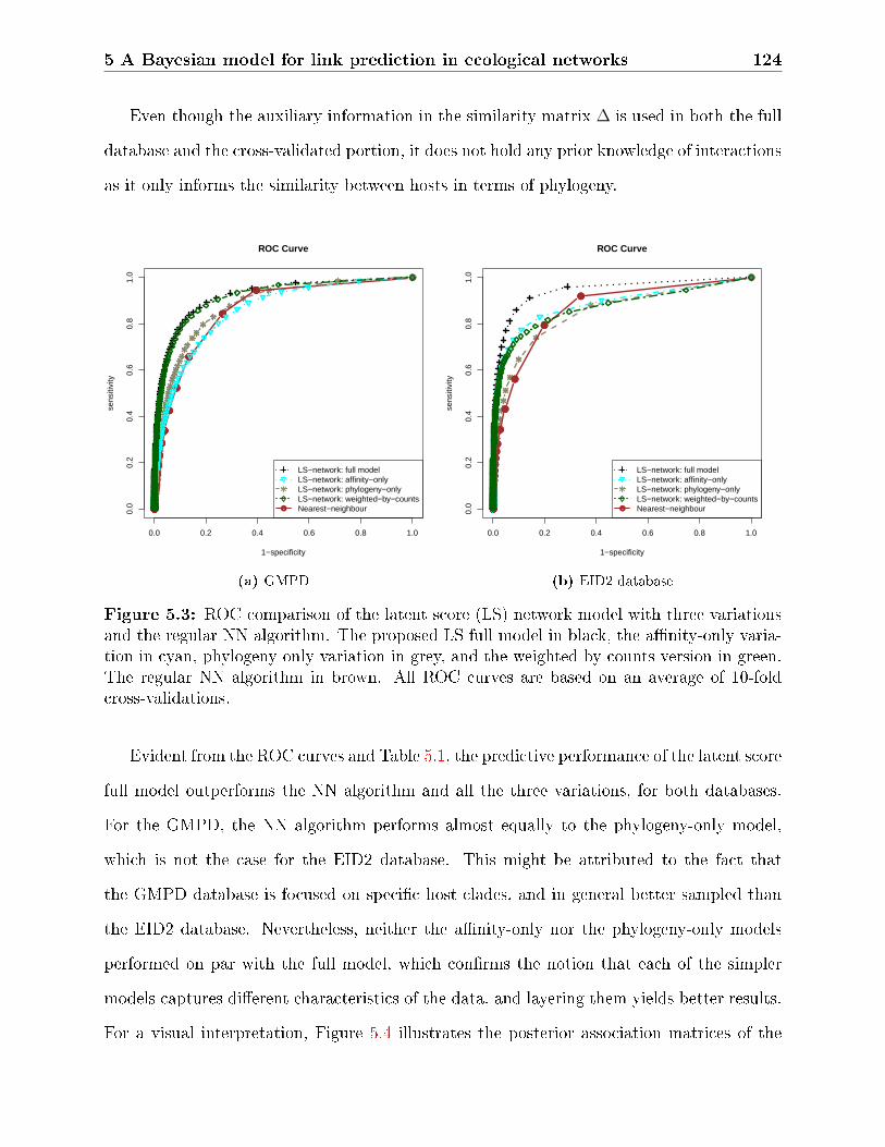
5 A Bayesian model for link prediction in ecological networks 124

Even though the auxiliary information in the similarity matrix ∆ is used in both the full

database and the cross-validated portion, it does not hold any prior knowledge of interactions

as it only informs the similarity between hosts in terms of phylogeny.

0.0 0.2 0.4 0.6 0.8 1.0

0.0

0.2

0.4

0.6

0.8

1.0

ROC Curve

1−specificity

sens

itivi

ty

LS−network: full modelLS−network: affinity−onlyLS−network: phylogeny−onlyLS−network: weighted−by−countsNearest−neighbour

(a) GMPD

0.0 0.2 0.4 0.6 0.8 1.0

0.0

0.2

0.4

0.6

0.8

1.0

ROC Curve

1−specificity

sens

itivi

ty

LS−network: full modelLS−network: affinity−onlyLS−network: phylogeny−onlyLS−network: weighted−by−countsNearest−neighbour

(b) EID2 database

Figure 5.3: ROC comparison of the latent score (LS) network model with three variationsand the regular NN algorithm. The proposed LS full model in black, the anity-only varia-tion in cyan, phylogeny-only variation in grey, and the weighted-by-counts version in green.The regular NN algorithm in brown. All ROC curves are based on an average of 10-foldcross-validations.

Evident from the ROC curves and Table 5.1, the predictive performance of the latent score

full model outperforms the NN algorithm and all the three variations, for both databases.

For the GMPD, the NN algorithm performs almost equally to the phylogeny-only model,

which is not the case for the EID2 database. This might be attributed to the fact that

the GMPD database is focused on specic host clades, and in general better sampled than

the EID2 database. Nevertheless, neither the anity-only nor the phylogeny-only models

performed on par with the full model, which conrms the notion that each of the simpler

models captures dierent characteristics of the data, and layering them yields better results.

For a visual interpretation, Figure 5.4 illustrates the posterior association matrices of the

5 A Bayesian model for link prediction in ecological networks 125

anity-only (5.4a,5.4d), phylogeny-only (5.4b,5.4e) and the full model (5.4c,5.4f) for the

GMPD and EID2 databases respectively. From the gures, the anity-only model did not

account for any neighbouring structure and results in hyperactive hosts, while the phylogeny-

only model based on host-neighbourhoods results in greater dierences among parasites.

The full model then combines characteristics of both the simpler models. Moreover, for

an analytical comparison, we followed the recommendation of Dem²ar (2006) to use the

two-sided Wilcoxon signed rank test on the 5-fold cross-validations, nonetheless, dierent

Bayesian comparison procedures are possible. We obtain a p-value of 0.043 and < 0.005

when comparing the full model with the NN algorithm for the GMPD and EID2 databases

respectively. Indicating, for a 5% level of signicance, the full model outperforms the NN

algorithm in both databases. When comparing the full model to all three variations, the

p-value is < 0.005 across the board in favour of the full model, as seen in Table 5.2. Except

when comparing to weighted-by-counts model in GMPD database, where the AUC results

are comparable.

Table 5.1: Area under the curve and prediction values for tested models

GMPD EID2Model AUC Prediction AUC PredictionLS-network: full model 92.11 0.84 94.29 0.87LS-network: anity-only 85.51 0.78 88.41 0.78LS-network: phylogeny-only 87.60 0.80 84.93 0.74LS-network: weighted-by-counts 91.56 0.83 87.13 0.74Nearest-neighbour 86.03 0.84 86.47 0.79

Table 5.2: Two-sided Wilcoxon signed rank test to compare model AUCs

Model GMPD EID2

full model 1.000 0.000 0.000 0.000 0.000 1.000 0.000 0.000 0.000 0.000phylogeny-only 0.043 1.000 0.000 0.000 0.000 0.043 1.000 0.000 0.000 0.000Nearest-neighbour 0.043 0.043 1.000 0.000 0.000 0.043 0.043 1.000 0.000 0.000anity-only 0.043 0.043 0.225 1.000 0.000 0.043 0.043 0.043 1.000 0.000weighted-by-counts 0.225 0.043 0.043 0.043 1.000 0.043 0.043 0.225 0.043 1.000

5 A Bayesian model for link prediction in ecological networks 126

parasites

host

s

5 45 90 140 195 250 305 360 415 470 525 580 635 690

250

220

200

180

160

140

120

100

8060

4020

(a) GMPD: anity-only

parasitesho

sts

5 45 90 140 195 250 305 360 415 470 525 580 635 690

250

220

200

180

160

140

120

100

8060

4020

(b) GMPD: phylogeny-only

parasites

host

s

5 45 90 140 195 250 305 360 415 470 525 580 635 690

250

220

200

180

160

140

120

100

8060

4020

(c) GMPD: full model

parasites

host

s

5 45 90 145 205 265 325 385 445 505 565 625 685 745

700

640

580

520

460

400

340

280

220

160

100

50

(d) EID2: anity-only

parasites

host

s

5 45 90 145 205 265 325 385 445 505 565 625 685 745

700

640

580

520

460

400

340

280

220

160

100

50

(e) EID2: phylogeny-only

parasites

host

s

5 45 90 145 205 265 325 385 445 505 565 625 685 745

700

640

580

520

460

400

340

280

220

160

100

50

(f) EID2: full model

Figure 5.4: Posterior associations matrix comparison: for the GMPD (top panel) and EID2(bottom panel), between the anity-only (left), phylogeny-only (middle) and full model(right).

5.4.4 Uncertainty in unobserved interactions

We improve on the latent score model by accounting for uncertainty in unobserved interac-

tions, as shown in Section 5.3. This addition increases the posterior predictive accuracy by

estimating the proportion of missing interactions in the observed data, and reducing scores

for unobserved interactions. Using the model in Section 5.3, we infer the false negative

rate g for both databases, using 10000 MCMC iterations with 2000 burn-in. The posterior

mean of g is found to be 0.34 for the GMPD, and 0.38 for the EID2 database, for posterior

histograms refer to Appendix Figure C.4. The EID2 false negative rate is larger than the

rate of the GMPD, which reects the dierences in search strategies and sources used in the

5 A Bayesian model for link prediction in ecological networks 127

creation of each database. Documented associations in the GMPD are identied through

systematic searches of common online reference databases to nd peer-reviewed articles that

support an interaction. EID2, on the other hand, identies associations that are supported

by information in genetic sequence databases and citations found in the biomedical related

search engine PubMed.

Incorporating the proportion of missing interactions is designed to improve posterior

predictive accuracy. To show that, we divided the databases into two sets, a training and

a validation set. Since associations in the GMPD are sourced only from peer-reviewed

articles, we were able to use information on article publication dates to create the two sets.

This mimics the discovery of interactions in the system rather than random hold-out of

observations. Taking the earliest annotated year for each association we set the training

set as all associations documented prior to and including 2004, and the validation set as all

associations up to 2010. Prior to and including 2004, there are 3462 pairs of documented

associations. By 2010, the associations increased to 3966, approximately a 15% increase. The

static EID2 database does not have any temporal information readily accessible, therefore

we created the training set by removing randomly 10% of the observed associations, where

the validation set holds all associations. This amounts to 3357 unique association pairs in

the training set and 3730 in the validation set.

For the training sets, we used an average of 5-fold cross-validations to estimate the

parameters of the model, where each fold ran for 10000 iterations with 2000 burn-in. Due to

the overlap between the two databases, we validated the model on distinct subsets of hosts

for each database. For the GMPD we used the Carnivora clade, and for the EID2 we used

the Rodentia clade.

Figure 5.5 illustrates the improvement in predictive accuracy between the models with g

and without g. For the GMPD-Carnivora the AUC is 0.935 and 0.843 for the models with

and without g, respectively. For the EID2-Rodentia the AUC is 0.899 and 0.832 for the

models with g and without g, respectively. In both cases, the model with g is a signicant

5 A Bayesian model for link prediction in ecological networks 128

0.0 0.2 0.4 0.6 0.8 1.0

0.0

0.2

0.4

0.6

0.8

1.0

ROC Curve

1−specificity

sens

itivi

ty

LS−network: with gLS−network: without g

(a) GMPD-Carnivora

0.0 0.2 0.4 0.6 0.8 1.0

0.0

0.2

0.4

0.6

0.8

1.0

ROC Curve

1−specificityse

nsiti

vity

LS−network: with gLS−network: without g

(b) EID2-Rodentia

Figure 5.5: Comparison of ROC curves for the model with g (black) and without g (grey),for GMPD-Carnivora on the left and the EID2-Rodentia on the right.

improvement.

Essentially, incorporating the proportion of missing interactions g reduces the overlap

in posterior probability densities between interacting and non-interacting pairs. To show

this, one can simply view the posterior histogram of log-probabilities of both categories, the

observed and unobserved interactions, for the model with and without g. For the model

with g, the overlap of the histogram of both probabilities is lower than the model without g,

which the partition clearer between the two categories. For an example, refer to Appendix

Figure C.5

Table 5.3 is a summary of AUC results when applying the two model variations to both

databases and discussed subsets. In all cases, incorporating g results in more accurate poste-

rior predictions. For the EID2 database, despite the higher value of g, the AUC dierence is

small. This might be attributed to the way the training set is designed, since the EID2 train-

ing set was created by random elimination of observed interactions compared to temporal

sub-setting for the GMPD. In particular, research documenting host-parasite associations

5 A Bayesian model for link prediction in ecological networks 129

may be driven by previous research ndings and this biased towards particular hosts or

parasites may be captured in the temporal structure of the database, but not by random

elimination. By applying the two-sided Wilcoxon signed rank test, we found the p-value to

be < 0.005 in favour of the model with g for both databases and subsets, thus signicant

prediction gains are attained when incorporating g.

Table 5.3: AUC comparison between models with g and without g on the GMPD and EID2databases and clade subsets

Model GMPD-Carnivora GMPD EID2-Rodentia EID2with g 0.935 0.924 0.899 0.938without g 0.843 0.891 0.832 0.916

For AUC results that include sub-models, refer to Appendix Tables C.2 and C.4.

Modelling uncertainty by incorporating the proportion of missing interactions certainly

improves the posterior prediction as seen in Table 5.3, where in all sets the AUC is higher

for models including g. In terms of the proportion of observed interactions recovered, the

results dier. Table 5.4 shows the percentage of observed interactions correctly predicted

in the held-out portion of the validation set (in parentheses) and in the full data, for each

database type and model. That is for the GMPD using the model with g, the percentage of

predicted interactions for documented associations from 2005 to 2010, is 0.683, and 0.832 for

all documented associations up to 2010. Using the simpler model without g, the equivalent

values are 0.788 and 0.811. For the GMPD-Carnivora both percentages only account for the

Carnivora host subset. For the EID2 database, when modelling with g, the percentage of

predicted interactions for the 10% held-out is 0.92, and 0.919 for the full database. When

modelling without g, the equivalent values are 0.92 and 0.85. It is clear that the model with

g outperforms in the predicted interactions of the full database, but lacks when it comes

to predicting the held-out portions in the validation set. The model without g simply over

estimates the amount of associations, which yields a higher recovery of observed interactions

in the held-out portion, but also predicts a greater number of unobserved interactions as

present, which reduces the AUC.

5 A Bayesian model for link prediction in ecological networks 130

Table 5.4: Percentage of observed interactions correctly predicted in the held-out portionof the validation set (in parentheses) and in the full data, for the GMPD and EID2 databases

Model GMPD-Carnivora GMPD EID2-Rodentia EID2with g (0.373) 0.827 (0.683) 0.832 (0.809) 0.825 (0.92) 0.919without g (0.573) 0.784 (0.788) 0.811 (0.681) 0.665 (0.92) 0.85

For more prediction results that include sub-models, refer to Appendix Tables C.3 and

C.5, and for more diagnostic plots and results, please refer to Appendix C.

5.5 Discussion

In this chapter we introduce a latent score model for link prediction in ecological networks

and illustrate it using two host-parasite networks. The proposed model is a combination of

two separate models, an anity based exchangeable random networks model (5.1) overlaid

with a Markov network dependence informed by phylogeny (5.3). The anity-only model is

characterized by independent anity parameters for each species, while the phylogeny-only

model is characterized by a scaled species similarity matrix. Both parts perform reasonably

well alone compared to the combined model, as shown in Figure 5.5. However, modelling with

only the anity parameters results in a highly dense posterior interaction matrix, in which

a slightly elevated anity parameter results in predicted interactions with all other species.

This situation is unlikely from a biological standpoint as species that are known to associate

with only particular evolutionary groups are predicted to associate with all others, regardless

of species identity. On the other hand, modelling using only the phylogenetic dependence

structure allows no independent inuence of the number of documented interactions per

species. By overlaying the anity-only model with a phylogeny-only dependence structure,

the posterior prediction is signicantly improved and the sparseness of the original interaction

matrix is preserved.

While we incorporated phylogeny as the dependence structure, the model can easily

accommodate dierent similarity matrices or types of dependence in an additive manner.

5 A Bayesian model for link prediction in ecological networks 131

For host-parasite networks, host traits or geographic overlap, or parasite similarity based

on phylogeny, taxonomy, or traits may improve prediction (Davies and Pedersen, 2008; Luis

et al., 2015; Pedersen et al., 2005). Introducing dierent similarity measures aects the

model characteristics in two ways: it changes the topology of the probability domain, and it

increases the number of parameters to estimate due to introduced scaling parameters. The

latter is easily integrated since the number of estimated parameters increases by one for each

new scaling parameter.

A particular dependence structure that does not require additional data is similarity

based on the number of shared interactions, as used in the NN algorithm (seen in Section

5.4.3). However, this method under-performed when compared to the phylogeny based simi-

larity. The magnitude of the scaling parameter for both databases indicates the utility of the

phylogenetic information. In host-parasite networks, parasite community similarity is often

well predicted by evolutionary distance among hosts (Davies and Pedersen, 2008; Gilbert

and Webb, 2007). In this case, the NN similarity is likely capturing some of the phyloge-

netic structure in the network and could be a reasonable approach if a reliable phylogeny is

unavailable. However, as phylogeny is estimated independently from the interaction data,

it will likely be more robust to incomplete sampling of the original network than NN type

dependence structures.

Many ecological networks are often based on presence-only data (Morales-Castilla et al.,

2015), where an unobserved interaction may be either present or absent. Thus, to account for

uncertainty in unobserved interactions we incorporate the proportion of missing interactions

in the observed data, which strengthens the posterior predictive accuracy of the model. We

additionally present a variation that includes a weighted-by-counts component, although, as

shown in Section 5.4.3, we nd the original model outperforms it. One might assume that

the count of peer-reviewed articles or unique genetic sequences reects the strength of the

underlying support. However, certain species, such as domesticated animals, or organisms

that are threats to public health, may receive signicantly more research interest (Wiethoelter

5 A Bayesian model for link prediction in ecological networks 132

et al., 2015). This elevated study eort may reveal additional interactions and increase

the number of studies reporting previously known associations. In the weighted-by-counts

model, these inated counts decrease overall predictive accuracy by estimating many weakly

supported interactions as absent. For example, an interaction between two rarely studied

species may be supported by a single valid piece of evidence, the strength of which is not

reected by the count of unique pieces of evidence.

While the intent of this research is to identify undocumented interactions, this model can

also account of uncertainty in missing interactions. In this case, the model may be used to

identify weakly supported interactions that are false positives or sampling artifacts in the

literature that may benet from additional investigation. We hope that this work inspires

new research on the modelling of host-parasite networks, and in particular, methods that

allow for the uncertainty in unobserved interactions. We believe frameworks such as ours

will be valuable tools for better understanding the structures of species interaction networks,

and could form an integral component of proactive surveillance systems for emerging diseases

(Farrell et al., 2013).

133

Appendices

134

Appendix A

Latent formulation and sampling

For an H × J matrix Z of interactions with no empty columns or rows, of h = 1, . . . , H

hosts, and j = 1, . . . J parasites, let γh > 0 be the anity parameter of host h , and

ρj > 0 for parasite j. Let ∆ be an H × H matrix that quanties pairwise similarities

between hosts, where higher values imply stronger correlations and 0 < ∆hk < 1 for all

h, k ∈ 1, . . . , H, h = k.

Suppose that the probability of an edge zhj conditional on all other edges Z−(hj) is dened

as

P(zhj = 1 | Z−(hj)) = 1− exp(−τhj), (A.1)

where τhj = γhρjδηhj and η is a scaling coecient of the similarity matrix.

To facilitate modelling, suppose that zhj is completely determined by a latent score shj,

such that

zhj =

⎧⎪⎪⎨⎪⎪⎩1 shj > 0

0 shj = 0.

with

P(zhj = 1 | Z−(hj)) = E[Ishj>0 | Z−(hj)] = P(shj > 0 | S−(hj)) = 1− exp(−τhj).

A Latent formulation and sampling 135

Such a characterization prompt a conditional joint distribution of the form

P(zhj = 1, shj | Z−(hj)) = P(zhj = 1 | shj)p(shj | S−(hj)) = p(shj | S−(hj))Ishj>0

P(zhj = 0, shj | Z−(hj)) = P(zhj = 0 | shj)p(shj | S−(hj)) = p(shj | S−(hj))Ishj=0.

(A.2)

Moreover, it can be veried that

p(shj | zhj,Z−(hj)) =

⎧⎪⎪⎨⎪⎪⎩1

1−exp(−τhj)p(shj | S−(hj))Ishj>0 zhj = 1

1exp(−τhj)

p(shj | S−(hj))Ishj=0 zhj = 0.

It remains to dene the distribution of shj | Z−(hj) to satisfy the property that

P(zhj = 1 | Z−(hj)) = 1− exp(−τhj) =∫Rp(s | S−(hj))Is>0ds.

One possible choice is the partitioned Gumbel density as

p(shj | S−(hj)) = τhj exp(−shj − τhje−shj)Ishj>0 + exp(−τhj)Ishj=0.

The latent score is only used as a modelling tool to make the joint distribution more

tractable, as

p(zhj, shj | Z−(hj)) =[τhj exp

(−(shj + τhje

−shj)

)Ishj>0

]zhj[exp (−τhj)Ishj=0

]1−zhj= τ

zhjhj exp

(−shj − τhje

−shj).

(A.3)

By construction, the neighbourhood structure represented by δηhj depends only on the

host phylogeny, hence, the joint distribution of each column of Z is independent of all others.

Since Z has no empty columns, assuming that zhj represent the rst observed interaction for

A Latent formulation and sampling 136

the j-th column Z. j, by conditioning the column joint distribution is

P(Z.j,S.j) =H∏h=1

(ρjγhδ

ηhj

)zhjexp

(− shjzhj − ρjγhδ

ηhje

−shjzhj)

= ρmj

j

[ H∏h=1

γzhjh

][ H∏h=1

(δηhj)zhj] exp(−

H∑h=1

shjzhj + ρjγhδηhje

−shjzhj

),

(A.4)

where δηhj =∑h−1

k=1 ∆hkzkj = δηhj −∑H

k=h+1 ∆hkzkj = δηhj − δηhj, and mj =∑H

h=1 zhj, with the

convention that δη1j = 1. The full joint distribution of Z is then

P(Z,S) =

[ J∏j=1

ρmj

j

][ H∏h=1

γnhh

][ J,H∏h,j=1

(δηhj)zhj] exp(−

J,H∑h,j=1

shjzhj + ρjγhδηhje

−shjzhj

), (A.5)

where nh =∑J

j=1 zhj.

For the priors π( . ) the posterior distribution of the anity parameters are

p(ρj| . ) ∝ ρmj

j exp

(− ρj

H∑h=1

γhδηhje

−shjzhj

)π(ρj)

∝ ρmj

j exp

(− ρj

H∑h=1

γhδηhje

−shjzhj

)exp

(ρj

H∑h=1

γhδηhje

−shjzhj

)π(ρj),

p(γh| . ) ∝ γnhh exp

(− γh

J∑j=1

ρjδηhje

−shjzhj

)exp

(γh

J∑j=1

ρj δηhje

−shjzhj

)π(γh).

(A.6)

Let tGumbel(τ, 1, 0

)be a zero-truncated Gumbel random variables with scale parameter

of 1, having the density

exp(−(s− τ + e−(s−τ))

1− exp(−eτ ) χ(0,∞)(s).

Sampling the posterior latent score follows:

shj | Z,ρ,γ, η ∼

⎧⎪⎪⎨⎪⎪⎩χ0 if zhj = 0

tGumbel

(log(γhρjδ

ηhj), 1, 0

)if zhj = 1,

(A.7)

A Latent formulation and sampling 137

where χ0 is an atomic measure at zero.

The joint distribution in (A.4) and (A.5) depends on the order of observations per j-th

parasite, (z1j, z2j, . . . , zHj). The dependence is omitted but implicitly assumed. That is, each

subscript hj should be σj(h)j, where σj : 0, . . . , H ↦→ 0, . . . , H is an independent permu-

tation of the order of observations for the j-th parasite. Nonetheless, the joint distribution

is valid for each xed permutation, and the model is run as so.

The joint distribution, in general, is not tractable, primarily due to the inuence of the

order of observations. This order-dependence could be partially omitted in a way similar to

the Ising model. In particular, if we let δηhj be parameterized in the exponential scale for

some similarity matrix ∆ as

δηhj = exp

(− η

H∑i=1

∆hizij

).

Then, the thirds product in (A.5) becomes

J∏j=1

H∏h=1

(δηhj)zhj =

J∏j=1

H∏j=1

exp

(− ηzhj

h−1∑i=1

∆hizij

)=

J∏j=1

exp

(− η

2

H∑h,k=1

zhj∆hkzkj

).

However, as mentioned earlier, this transformation only partially relaxes the inuence

of order dependence, as it only aects the third product of (A.5) and not the dependence

seen in the exponential part. Moreover, the exponential scale transformation above alters the

interpretation of the neighbourhood structure in (5.2). Initially, δηhj was strictly non-negative,

where it penalizes the expected score for values less than one and complements it for values

larger than one. On the other hand, the exponential score transformation only penalizes the

expected score, as δηhj takes values strictly within (0, 1). We nd the parametrization in (5.2)

to have a better prediction performance.

A Latent formulation and sampling 138

A.1 Existence of the joint distribution

Theorem 14. (Hammersley-Cliord,(Robert and Casella, 2013)) Under marginal positively

conditions, the joint distribution of random variables Z = (z1, z2, . . . , zn) is proportional to

P(X)

P(X∗)=

n∏i=1

P(xi | x1, . . . , xi−1, x∗i+1, . . . , x

∗n)

P(x∗i | x1, . . . , xi−1, x∗i+1, . . . , x∗n)

(A.8)

where x∗i are xed observations, for example x∗i = 1.

In regards to conditional probability in (A.1), assume the phylogeny-only model where

τhj = δηhj, and δηhj as in (5.2). Since each column of Z is independent, it suces to show that

the joint distribution exist for each column. Applying the Hammersley-Cliord theorem, we

haveP(zhj | z1j, . . . , z(h−1)j, z

∗(h+1)j, z

∗Hj)

P(z∗hj | z1j, . . . , z(h−1)j, z∗(h+1)j, z∗Hj)

=[ exp(−τhj)1− exp(−τhj)

]1−zhj,

where z∗hj = 1 and

τhj =h−1∑i=1

∆ηhizij +

H∑i=h+1

∆ηhi, τ1j =

H∑j=2

∆ηhi, τHj =

H−1∑j=1

∆ηhizij.

Essentially, by removing the event of no interactions, as zh. = (0, 0, . . . , 0), and setting

τhj = 1 whenever it is 0, by Hammersley-Cliord theorem the joint distribution exists.

A.1.1 Parametrization using an exponential distribution

Rather than using a Gumbel distribution, one can achieve an equivalent parametrization

using the exponential distribution. Suppose that zhj is completely determined by a latent

variable uhj, such that

zhj =

⎧⎪⎪⎨⎪⎪⎩1 uhj < 1

0 uhj = 1.

A possible choice for the distribution of uhj | Z−(hj) is the density of a partitioned

A Latent formulation and sampling 139

exponential distribution, as

p(uhj | Z−(hj)) = τhj exp

(− τhjuhj

)Iuhj<1 + exp

(− τhj

)Iuhj=1.

where τhj = γhρjδηhj. The joint distribution becomes

p(zhj, uhj | Z−(hj)) =[τhj exp

(−τhjuhj

)Iuhj<1

]zhj[exp (−τhj)Iuhj=1

]1−zhj= τ

zhjhj exp

(−τhjuhj

).

A.2 Latent score sampling with uncertainty

By modelling the uncertainty parameter g as

p(zhj = 0 | shj, g) =

⎧⎪⎪⎨⎪⎪⎩1, if shj = 0

g, if shj > 0.

One arrives at the conditional joint distributions

P(zhj = 1, shj | g,Z−(hj)) = P(zhj = 1 | g, shj)p(shj | Z−(hj))

= p(shj | Z−(hj))Ishj>0

P(zhj = 0, shj | g,Z−(hj)) = P(zhj = 0 | g, shj)p(shj | Z−(hj))

= p(shj | Z−(hj))[gIshj>0 + Ishj=0

].

(A.9)

The conditional sampling of the latent truncated score variable shj becomes

p(shj | zhj,Z−(hj), g) =P(zhj | shj, g) . p(shj | Z−(hj))∫P(zhj | s, g) . p(s | Z−(hj))ds

= C . p(shj | Z−(hj)),

A Latent formulation and sampling 140

Such that

C =P(zhj | shj, g)∫

P(zhj | s, g) . p(s | Z−(hj))ds

=P(zhj | shj, g)∫

s>0P(zhj | s, g) . p(s | Z−(hj))ds+

∫s≤0

P(zhj | s, g) . p(s | Z−(hj))ds

=

⎧⎪⎪⎨⎪⎪⎩P(zhj |shj ,g)∫

s>0 1 . p(s|Z−(hj))ds+∫s≤0 0 . p(s|Z−(hj))ds

, when zhj = 1,

P(zhj |shj ,g)∫s>0 g . p(s|Z−(hj))ds+

∫s≤0 1 . p(s|Z−(hj))ds

, when zhj = 0,

=

⎧⎪⎪⎪⎪⎪⎪⎪⎪⎪⎪⎨⎪⎪⎪⎪⎪⎪⎪⎪⎪⎪⎩

1ψ(shj)

, shj > 0, zhj = 1,

0, shj = 0, zhj = 1,

ggψ(shj)+1−ψ(shj)

, shj > 0, zhj = 0,

1gψ(shj)+1−ψ(shj)

, shj = 0, zhj = 0,

where ψ(shj) =∫∞0

p(s | S−(hj), γh, ρj, η)ds = 1− exp

(−γhρjδηhj

).

Moreover, sampling the uncertainty variable is done by using the conditional distribution

as

P(g | S,Z) ∝ P(Z | S, g) . P(g) ∝ gN−+(1− g)N++ ,

where N−+ = #(h, j) : zhj = 0, shj > 0, N++ = #(h, j) : zhj = 1, shj > 0.

141

Appendix B

Details on the MCMC algorithm

Given the observed matrix Z to approximate the posterior density p(ρ,γ, η, ϕρ, ϕγ, ϕη|Z),

where ϕx is the gamma hyperparameters for the x parameter as ϕx = (αx, τx). Note that

each interaction zhj depends only on row h and column j via the parameters γh and ρj,

and on η via the dependency structure δ. Hence, one can update the parameters related

to the diagonal zhh : h = 1, . . . , H in parallel while retaining convergence conditions.

Generalizing this allows the parallel update of the parameters related to the i = 0, . . . , J − 1

diagonals

zh,(h+i) mod J : h = 1, . . . , H,

in the following steps, using Metropolis-Hasting steps:

1) update ϕρ, ϕγ and ϕη given (ρ,γ, η),

2) update ρ = (ρj)Jj=1 in parallel given (ϕρ, ϕγ, ϕη,γ, η) via (A.6),

3) update γ = (γh)Hh=1 in parallel given (ϕρ, ϕγ, ϕη,ρ, η) via (A.6),

4) update η given (ϕρ, ϕγ, ϕη,ρ,γ) with a proposal acceptance probability ofmin(1, a), where

a =

[ J,H∏h,j=1

(δηhjδηhj

)zhj]exp

(−

J,H∑h,j

ρjγhe−shjzhj(δηhj − δηhj)

).

B Details on the MCMC algorithm 142

A new proposal of η is sampled from a log-normal distribution as q(η | η) = lognormal(log(η), σ2η),

given a at prior.

5) update the latent variables of the diagonal s∗h,(h+i) mod J : h = 1, . . . , H as

shj | Z,ρ,γ, η ∼

⎧⎪⎪⎨⎪⎪⎩χ0 if zhj = 0

tGumbel

(log(γhρjδ

ηhj), 1, 0

)if zhj = 1,

(h, j) ∈ (h, x) : x = (h+ i) mod J for diagonal i,

where γ∗ ≈ 0.5772 is the Euler-Mascheroni constant, and χ0 is an atomic measure at

zero. tGumbel(τ, 1, 0) is a zero-truncated Gumbel distribution with a probability density

function as in (A.7).

Updating the uncertainty parameter g:

When correcting for uncertainty, just after step 4) above, sample g given (ρ,γ, η) using

a direct sample from a Beta(N−+, N++) distribution. That is, for h = 1, . . . , H and k =

1, . . . , J ,

N−+ = #(h, k) : zhk = 0, shk > 0, N++ = #(h, k) : zhk = 1, shk > 0.

Step 5) becomes

shj | Z,ρ,γ, η, g ∼

⎧⎪⎪⎪⎨⎪⎪⎪⎩1

θ(g,shj)χ0 +

gθ(g,shj)

tGumbel

(log(γhρjδ

ηhj), 1

)if zhj = 0

tGumbel

(log(γhρjδ

ηhj), 1

)if zhj = 1,

(h, j) ∈ (h, x) : x = (h+ i) mod J for diagonal i.

Updating hyperparameters ϕρ, ϕγ:

Since the host and parasite priors are characterized with a two parameter Gamma distri-

B Details on the MCMC algorithm 143

butions (α, τ), we will omit the subscripts and work with a general hyperparameter update

mechanism. Independently, for each of the parameter sets ϕρ and ϕγ given the other pa-

rameters and the latent variables ϕ∗ = (ρ,γ, η,S), update them using a Metropolis-Hasting

step, with proposals ϕ = (α, τ) from q(α, τ | α, τ). The acceptance probability is min(1, a),

where

a =p(ϕ | ϕ∗)

p(ϕ | ϕ∗)× q(ϕ | ϕ)q(ϕ | ϕ)

=

∏Nx

i=1

∫R+

p(xi | ϕ, ϕ∗)p(ϕ)dxi∏Nx

i=1

∫R+

p(xi | ϕ, ϕ∗)p(ϕ)dxi× q(ϕ | ϕ)q(ϕ | ϕ)

.

The symbols ρ and γ substitute for x above, where Nρ = J and Nγ = H. The joint

distribution in (5.8) is independent of the hyperparameters, thus it is left out.

Independent proposals are used, q(ϕ = (α, τ) | α, τ) = q(α | α)q(τ | τ), where

q(α|α) ∼ lognormal(log(α), σ2α),

q(τ |τ) ∼ lognormal(log(τ), σ2τ ).

With improper priors as

p(α, τ) = p(α)p(τ), p(α) ∝ 1

α, p(τ) ∝ 1

τ,

The general form of the acceptance probability a simplies to

a =Nx∏i=1

[∫R+

p(xi | α, τ , ϕ∗)dxi∫R+

p(xi | α, τ, ϕ∗)dxi

]× ατ

ατ× ατ

ατ=

Nx∏i=1

∫R+

p(xi | α, τ , ϕ∗)dxi∫R+

p(xi | α, τ, ϕ∗)dxi.

Such that, the acceptance probability a for each case is:

• ϕγ = (αγ, τγ) as

a =

[ταγγ

ταγγ

Γ(αγ)

Γ(αγ)

]H H∏h=1

Γ(nh + αγ)

Γ(nh + αγ)

(τγ +Ψ′h)nh+αγ

(τγ +Ψ′h)nh+αγ

, Ψ′h =

J∑j=1

ρjδηhje

−shj , nh =J∑j=1

zhj,

B Details on the MCMC algorithm 144

• ϕρ = (αρ, τρ) as

a =

[τ αρ

ταρ

Γ(αρ)

Γ(αρ)

]J J∏j=1

Γ(mj + αρ)

Γ(mj + αρ)

(τρ +Ψj)mj+αρ

(τρ +Ψj)mj+αρ, Ψj =

H∑h=1

γhδηhje

−shj , mj =H∑h=1

zhj.

145

Appendix C

Additional results

C.1 Posterior distributions

Figure C.1 shows posterior boxplots for the parameters with the 80 highest posterior medians

and the posterior distribution of the scaling parameter η, for the GMPD (top panel) and

EID2 (bottom panel). As shown, for the GMPD, the parasite parameters (ρ) vary moder-

ately, which reects the balance of column densities in the left-ordered interaction matrix in

Chapter Figure 5.1. The host parameters (γ) show more variation, which reects that some

hosts are more likely to interact with parasites, or have been more intensively studied. In

the EID2 database, the variation among the hosts is more prominent, which conrms our

earlier observation that row densities of the EID2 interaction matrix are less balanced (see

Chapter Figure 5.1). The ρ parameters on the other hand, do not show much variation in

either database, as seen by the column densities of the interaction matrices.

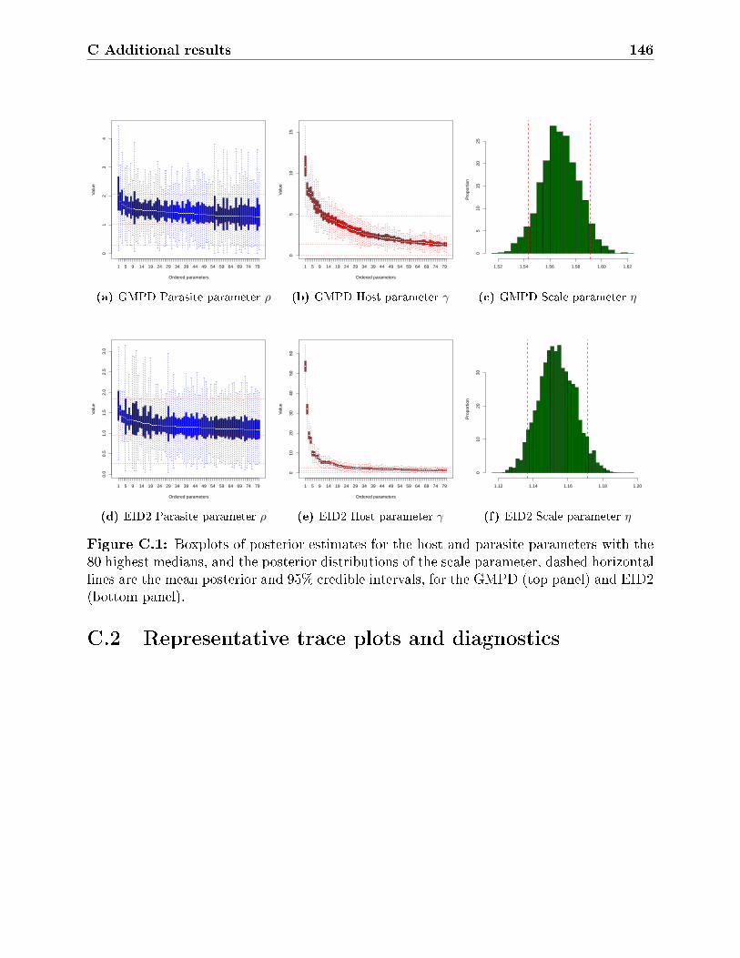
C Additional results 146

1 5 9 14 19 24 29 34 39 44 49 54 59 64 69 74 79

01

23

4

Ordered parameters

Val

ue

(a) GMPD Parasite parameter ρ

1 5 9 14 19 24 29 34 39 44 49 54 59 64 69 74 79

05

1015

Ordered parametersV

alue

(b) GMPD Host parameter γ

Pro

port

ion

1.52 1.54 1.56 1.58 1.60 1.62

05

1015

2025

(c) GMPD Scale parameter η

1 5 9 14 19 24 29 34 39 44 49 54 59 64 69 74 79

0.0

0.5

1.0

1.5

2.0

2.5

3.0

Ordered parameters

Val

ue

(d) EID2 Parasite parameter ρ

1 5 9 14 19 24 29 34 39 44 49 54 59 64 69 74 79

010

2030

4050

60

Ordered parameters

Val

ue

(e) EID2 Host parameter γ

Pro

port

ion

1.12 1.14 1.16 1.18 1.20

010

2030

(f) EID2 Scale parameter η

Figure C.1: Boxplots of posterior estimates for the host and parasite parameters with the80 highest medians, and the posterior distributions of the scale parameter, dashed horizontallines are the mean posterior and 95% credible intervals, for the GMPD (top panel) and EID2(bottom panel).

C.2 Representative trace plots and diagnostics

C Additional results 147

0 2000 4000 6000 8000 10000

45

67

8

Iteration

Hos

t

0 2000 4000 6000 8000 10000

1.0

1.4

1.8

2.2

Iteration

Par

asite

0 2000 4000 6000 8000 10000

1.52

1.56

1.60

Iteration

Sca

le

(a) GMPD

0 2000 4000 6000 8000 10000

1.8

2.2

2.6

3.0

Iteration

Hos

t

0 2000 4000 6000 8000 10000

1.0

1.4

1.8

2.2

Iteration

Par

asite

0 2000 4000 6000 8000 10000

1.12

1.16

IterationS

cale

(b) EID2

Figure C.2: Trace plots for the GMPD and EID2: host (top) and parasite (middle) ofhighest median posterior, and the similarity matrix scaling parameter (bottom).

0 20 40 60 80 100

0.0

0.4

0.8

Lag

AC

F

Host − most active

Effective sample size: 1639

0 20 40 60 80 100

0.0

0.4

0.8

Lag

AC

F

Parasite − most active

Effective sample size: 1881

0 20 40 60 80 100

0.0

0.4

0.8

Lag

AC

F

Scale parameter

Effective sample size: 404

(a) GMPD

0 20 40 60 80 100

0.0

0.4

0.8

Lag

AC

F

Host − most active

Effective sample size: 1000

0 20 40 60 80 100

0.0

0.4

0.8

Lag

AC

F

Parasite − most active

Effective sample size: 885

0 20 40 60 80 100

0.0

0.4

0.8

Lag

AC

F

Scale parameter

Effective sample size: 330

(b) EID2

Figure C.3: ACF plots and eective sample sizes for the GMPD and EID2: host (top) andparasite (middle) of highest median posterior, and the similarity matrix scaling parameter(bottom).

C Additional results 148

C.3 Parameter numerical results

Table C.1: Posterior means, Monte Carlo standard errors and credible intervals for thehighest anity parameters and the scale parameter.

GMPD networkParameter Estimate standard dev 95% credible intervalρ(1) 2.18 0.94 (0.93, 3.91)ρ(2) 1.84 0.48 (1.13, 2.68)ρ(3) 1.81 0.64 (0.88, 2.97)ρ(4) 1.70 0.51 (0.97, 2.62)ρ(5) 1.69 0.20 (1.38, 2.04)γ(1) 10.88 1.87 (7.94, 14.01)γ(2) 8.11 1.18 (6.25, 10.15)γ(3) 7.69 0.82 (6.39, 9.08)γ(4) 7.62 1.17 (5.81, 9.61)γ(5) 7.09 1.01 (5.47, 8.86)η 1.57 0.01 (1.54, 1.59)

EID2 networkParameter Estimate standard dev 95% credible intervalρ(1) 1.70 0.54 (0.92, 2.68)ρ(2) 1.56 0.18 (1.28, 1.87)ρ(3) 1.45 0.64 (0.55, 2.63)ρ(4) 1.43 0.22 (1.09, 1.8)ρ(5) 1.42 0.67 (0.52, 2.67)γ(1) 53.59 3.90 (47.41, 60.13)γ(2) 32.10 3.67 (26.2, 38.06)γ(3) 18.95 2.80 (14.68, 23.85)γ(4) 16.55 2.62 (12.42, 21.08)γ(5) 9.83 1.78 (7.09, 12.87)η 1.15 0.01 (1.14, 1.17)

C Additional results 149

C.4 Uncertainty - histograms

Posterior estimate of g for the GMP−Carnivora database

Fre

quen

cy

0.20 0.25 0.30 0.35 0.40 0.45

010

030

050

0

Posterior estimate of g for the GMP−Carnivora database

Fre

quen

cy

0.1 0.2 0.3 0.4 0.5 0.6

010

030

050

0

Figure C.4: Posterior histogram for g for the GMPD (left) and EID2 (right) databases.

Figure C.5 is the histogram of the posterior log-probabilities when using the model with-

out g (left), and the model with g (right), for the GMPD-Carnivora subset. For the model

without g, the right mode (cyan), is the histogram of the posterior log-probabilities of all the

observed interactions in the 2010 validation set, while the left mode (pink), is the histogram

of the posterior log-probabilities of unobserved interactions. For the model with g, the

overlap of the posterior log-probabilities of the two categories, observed and unobserved, is

signicantly reduced by lowering scores for the unobserved interactions. This causes a clearer

partition in probabilities between the two categories, and only unobserved interactions with

very high posterior probability are then classied as possible interactions.

C Additional results 150

Log of probability

Den

sity

−10 −8 −6 −4 −2 0

0.0

0.1

0.2

0.3

Observed associationsUnobserved associations

(a) without g

Log of probability

Den

sity

−10 −8 −6 −4 −2 0

0.0

0.1

0.2

0.3

Observed associationsUnobserved associations

(b) with g

Figure C.5: Comparison in posterior log-probability between observed and unobservedinteractions, for the model without g (left) and with g (right), for the GMPD-Carnivoradatabase.

C.5 Interaction matrices for subsets - Carnivora and Ro-

dentia

parasites

host

s

5 25 50 75 100 130 160 190 220 250 280 310 340

110

100

9080

7060

5040

3020

101

(a) GMPD-Carnivora

parasites

host

s

5 25 50 75 100 130 160 190 220 250 280 310 340

110

100

9080

7060

5040

3020

101

(b) Without g

parasites

host

s

5 25 50 75 100 130 160 190 220 250 280 310 340

110

100

9080

7060

5040

3020

101

(c) With g

Figure C.6: Association matrices of the whole GMPD-Carnivora subset: Observed (left),posterior for the model without g (middle), posterior for the model with g (right).

C Additional results 151

parasites

host

s

5 15 25 35 45 55 65 75 85 95 105 115 125

9080

7060

5040

3020

10

(a) EID2-Rodentia

parasites

host

s

5 15 25 35 45 55 65 75 85 95 105 115 125

9080

7060

5040

3020

10(b) Without g

parasites

host

s

5 15 25 35 45 55 65 75 85 95 105 115 125

9080

7060

5040

3020

10

(c) With g

Figure C.7: Association matrices of the whole EID2-Rodentia subset: Observed (left),posterior for the model without g (middle), posterior for the model with g (right).

C.6 ROC with and without g for full GMPD and EID2

databases

0.0 0.2 0.4 0.6 0.8 1.0

0.0

0.2

0.4

0.6

0.8

1.0

ROC Curve

1−specificity

sens

itivi

ty

LS−network: with gLS−network: without g

(a) GMPD

0.0 0.2 0.4 0.6 0.8 1.0

0.0

0.2

0.4

0.6

0.8

1.0

ROC Curve

1−specificity

sens

itivi

ty

LS−network: with gLS−network: without g

(b) EID2

Figure C.8: Comparison of ROC curves for the full dataset, for the models with(out) g.

C Additional results 152

Table C.2: AUC comparison between models with g and without g, on the GMPD databasesand clade subsets, with dierent variations of the model

Model GMPD-Carnivora GMPD GMPD Anity GMPD Phylogenywith g 0.935 0.924 0.926 0.853without g 0.843 0.891 0.856 0.825

Table C.3: Percentage of observed interactions correctly predicted in the held-out portionof the validation set (in parentheses) and in the full data, for the GMPD database

Model GMPD-Carnivora GMPD GMPD Anity GMPD Phylogenywith g (0.373) 0.827 (0.683) 0.832 (0.437) 0.824 (0.728) 0.803without g (0.573) 0.784 (0.788) 0.811 (0.607) 0.796 (0.698) 0.726

parasites

host

s

5 45 90 140 195 250 305 360 415 470 525 580 635 690

250

220

200

180

160

140

120

100

8060

4020

(a) GMPD without g

parasites

host

s

5 45 90 140 195 250 305 360 415 470 525 580 635 690

250

220

200

180

160

140

120

100

8060

4020

(b) GMPD with g

parasites

host

s

5 45 90 145 205 265 325 385 445 505 565 625 685 745

700

640

580

520

460

400

340

280

220

160

100

50

(c) EID2 without g

parasites

host

s

5 45 90 145 205 265 325 385 445 505 565 625 685 745

700

640

580

520

460

400

340

280

220

160

100

50

(d) EID2 with g

Figure C.9: Posterior association matrices for the full datasets.

C Additional results 153

Table C.4: AUC comparison between models with g and without g, on the EID2 databasesand clade subsets, with dierent variations of the model

Model EID2-Rodentia EID2 EID2 Anity EID2 Phylogenywith g 0.899 0.938 0.942 0.845without g 0.832 0.916 0.913 0.801

Table C.5: Percentage of observed interactions correctly predicted in the held-out portionof the validation set (in parentheses) and in the full data, for the EID2 database

Model EID2-Rodentia EID2 EID2 Anity EID2 Phylogenywith g (0.809) 0.825 (0.92) 0.919 (0.893) 0.934 (0.847) 0.822without g (0.681) 0.665 (0.92) 0.85 (0.834) 0.797 (0.786) 0.666

C Additional results 154

C.7 Percentage of recovered pairwise interactions

One of the ways to compare model performance other than the ROC curve is to look at

predictive performance by measuring the proportion of recovered true interactions in the

data. To show this, for each model, sort descendingly all pairwise interactions based on their

posterior predictive probabilities. Count the number of true interactions that have been

recovered within the x pairs with highest probabilities. Scaling x from 1 to 1000 to get the

following model comparative plots.

0 200 400 600 800 1000

020

040

060

080

0

Number of validated pairwise interactions

Num

ber

of r

ecov

ered

pai

rwis

e in

tera

ctio

ns

Full model with uncertaintyFull modelAffinity−only with uncertaintyAffinity−onlyPhylogeny−only with uncertaintyPhylogeny−onlyx=y

(a) GMPD

0 200 400 600 800 1000

010

020

030

040

050

060

070

0

Number of validated pairwise interactions

Num

ber

of r

ecov

ered

pai

rwis

e in

tera

ctio

ns

Full model with uncertaintyFull modelAffinity−only with uncertaintyAffinity−onlyPhylogeny−only with uncertaintyPhylogeny−onlyx=y

(b) EID2

Figure C.10: Number of pairwise recovered interactions from the original data.

C Additional results 155

C.8 Posterior degree distribution

+

+

+ +

+

+

++

+

+

+

+

+

+

+++

++

++

++

+

++

+

+

+

++

+

+

+

+

+

+

+

++

++++++

+

++

+

++++++++++++

1 2 5 10 20 50 100 200

12

510

2050

100

200

500

Degree

Num

ber

of N

odes

+ Hosts

Estimated

(a) Hosts - full model

*

*

*

*

*

**

*

**

*

*

**

*

*

**

**

****

**

******

1 2 5 10 20 50 100 200

12

510

2050

100

200

500

Degree

Num

ber

of N

odes

* Parasites

Estimated

(b) Parasites - full model

+

+

+ +

+

+

++

+

+

+

+

+

+

+++

++

++

++

+

++

+

+

+

++

+

+

+

+

+

+

+

++

++++++

+

++

+

++++++++++++

1 2 5 10 20 50 100 200

12

510

2050

100

200

500

Degree

Num

ber

of N

odes

+ Hosts

Estimated

(c) Hosts - full model with g

*

*

*

*

*

**

*

**

*

*

**

*

*

**

**

****

**

******

1 2 5 10 20 50 100 200

12

510

2050

100

200

500

Degree

Num

ber

of N

odes

* Parasites

Estimated

(d) Parasites - full model with g

Figure C.11: Comparison of degree distribution on log-scale, for the full model (withoutaccounting for uncertainty) and the model with g, GMPD dataset.

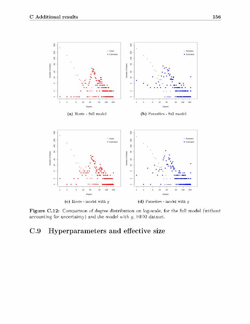
C Additional results 156

+

+

+

+

+ +

++

++++

+

++

++++

++

+

+

+

+

+

+++++++++++++

1 2 5 10 20 50 100 200

12

510

2050

100

200

500

Degree

Num

ber

of N

odes

+ Hosts

Estimated

(a) Hosts - full model

*

*

*

*

*

**

*

*

* **

**

*

**

*

*

*

********

*

**

1 2 5 10 20 50 100 200

12

510

2050

100

200

500

Degree

Num

ber

of N

odes

* Parasites

Estimated

(b) Parasites - full model

+

+

+

+

+ +

++

++++

+

++

++++

++

+

+

+

+

+

+++++++++++++

1 2 5 10 20 50 100 200

12

510

2050

100

200

500

Degree

Num

ber

of N

odes

+ Hosts

Estimated

(c) Hosts - model with g

*

*

*

*

*

**

*

*

* **

**

*

**

*

*

*

********

*

**

1 2 5 10 20 50 100 200

12

510

2050

100

200

500

Degree

Num

ber

of N

odes

* Parasites

Estimated

(d) Parasites - model with g

Figure C.12: Comparison of degree distribution on log-scale, for the full model (withoutaccounting for uncertainty) and the model with g, EID2 dataset.

C.9 Hyperparameters and eective size

C Additional results 157

0 2000 4000 6000 8000

0.0

0.1

0.2

0.3

0.4

Expected value of host affinity

Iteration

Hos

ts

0 2000 4000 6000 8000

010

2030

40

Expected value of parasite affinity

Iteration

Par

asite

s

Figure C.13: Trace plots of convergence of three chains started at dierent values for theexpected value of the hyperparameter for the GMPD dataset

158

Chapter 6

Conclusion and future research

This thesis has contributed to two sub-elds of statistical network analysis, one which is

modelling of random graphs, and the other on link prediction. On the former, this work has

proposed a new way of modelling decomposable graphs, which is achieved by adopting a non-

classical representation of decomposable graphs as deterministic functions of bipartite point

processes. On link prediction, this work has adopted methods of measuring the proportion of

missing link at the data source and applied it to correct for link prediction in presence-only

data.

Adopting from the recent work on models for random graphs, Chapter 3 proposed a

framework for modelling decomposable graphs that is driven by node specic anity pa-

rameters. Rather than modelling the probability of an edge forming between two nodes,

the proposed framework models the probability of nodes attaining membership in maximal

cliques of the graph. The maximal cliques are represented by latent communities that are

connected into a tree, mimicking that of the junction tree representation of decomposable

graphs. The bipartite interactions between the graph nodes and those latent communities

can be mapped deterministically to an adjacency matrix of a decomposable graph.

The adopted representation of decomposable graphs yields simple Markov update steps.

Conditional on the latent clique communities the node-clique relationship is assigned, and

6 Conclusion and future research 159

iteratively, the tree connectivity of the communities is updated according to their node

memberships. The adopted iterative procedure is native to many models of decomposable

graphs, due to their conditional dependency structure. Section 3.4 illustrated two sampling

mechanism for the proposed model, one based on sequential sampling with nite steps, and

the other based on a Markov stopped process. A lower bound of mixing time for the Markov

stopped process are specied. The bipartite representation of decomposable graphs permits

an easy computation of the expected number of maximal cliques per node, which is the topic

of Section 3.7.

One of the main benets of the proposed decomposable graphs framework of Chapter 3, is

the new application of sub-clustering, shown in Chapter 4. The bipartite representation can

easily be extended to account for subgraphs (sub-cliques) of maximal cliques, adding much

richness to the model. In classical settings, one models solely the decomposable graphs,

the proposed model, adds to that by exibly modelling the latent dynamics forming within

each maximal clique. Nonetheless, introducing sub-clustering to the model comes with ex-

tra complexities related to the dynamics between maximal and sub-maximal cliques. Few

methods exists in modelling this dynamics, this work adopted a method that utilizes the

continuity nature of the specic community anity parameters. Contrary to the treatment

of decomposable graphs in Chapter 3, allowing for sub-clustering requires a series of rules

addressing the change in the junction tree after every (dis)connect move. In some update

steps, a maximal clique might become sub-maximal and the opposite, varying the size of the

junction tree at every step. A major part of this work is dedicated to such update rules.

On the second area of contribution of this work, Chapter 5 introduced a Bayesian latent

score model for link prediction in presence-only networks. The proposed model assigns scores

on observed edges of a network in an attempt to rank edges from the most probable down

the least. On the rst instance, the model adopts classical anity based representations

of networks. To improve the scoring eciency the model is augmented with an informed

Markov random eld component, that also only depends on observed links. Since it is hard

6 Conclusion and future research 160

to know the exact number of actual true interactions from forbidden ones, drawing on some

of the work of Jiang et al. (2011), a measure of uncertainty is built which attempts to

estimate the false negative rate on the data source. This rate is then used to gauge the

predicted number of potential interactions. The model is validated using two host-parasite

networks constructed from published databases, the Global Mammal Parasite Database and

the Enhanced Infectious Diseases database, each with thousands of pairwise interactions.

6.1 Future research

The following is a list of future research directions.

• Bounds for mixing times: Chapter 3, Lemma 2 specied the lower bound of the mix-

ing time for the MCMC method of the proposed framework for decomposable graphs.

The lemma depends on the structure of the junction tree, through the component∑k 1/Γk. A possible research direction is to generalize this lower bound to depend on

a general measure of tree densities, which could be assumed on the junction tree of the

graph. Arriving at an expression for the upper bound would also be helpful.

• Expectation results on decomposable graphs: Assuming that the junction tree

of the graph is a d-regular tree, Section 3.7 gave an exact expression for the expected

number of maximal cliques per node. This result could be possibly extended to column-

wise expectations, as the expected size of a maximal clique. In addition, the given

expectation depends on some tree quantities, for example the number of edges of each

tree node, and the length of the tree. It is desired to have an expression that only

depends on general tree measures, which could be extended to general non-regular

trees.

• A second sub-clustering framework: Chapter 4 illustrated a new application of

decomposable graphs, motivated by a sub-clustering method. This method depends

6 Conclusion and future research 161

on the latent communities (θ′1, θ′2, . . . ) being classied into maximal and sub-maximal

cliques, the latter is treated as sub-clusters. In Chapter 3, those latent communities are

all assumed to represent maximal cliques. A possible research direction is to adopt a

second sub-clustering method, which is in between the proposed sub-clustering method

of Chapter 4 and the initial treatment of decomposable graphs of Chapter 3. In par-

ticular, Proposition 1 shows that by using the boundary and neighbouring sets of (3.7)

in the Markov update step of (3.12), the graph resulting from the mapping in (3.10) is

decomposable, though, not all active cliques in the biadjacency representation are max-

imal. In such a case, the non-empty non-maximal cliques can be seen as sub-clusters.

This denition of sub-clusters might lead to less complex update steps than the ones

in Chapter 4. However, the interpretation of sub-clusters diers, since as more nodes

join the graph, the non-empty non-maximal cliques are potentially maximal, which is

not the case in the proposed model of Chapter 4.

• Hubs of authority using decomposable graphs: The work of Chapter 5 proposed

a link prediction model for presence-only data. To account for the uncertainty in

missing interactions, a mechanism is built to account for the proportion of missing link

in the data source. This rate is then used to gauge the predicted number of potential

interactions. The motivational data example are host-parasite networks, which are

constructed from documented interactions based on peer-reviewed articles. Using the

time of publication and authorship information it is possible to integrate the work

done on decomposable graphs in accounting for uncertainty in missing interactions.

For example, by clustering authors on dierent types of interactions or host-interest

groups. Each cluster could be dened as a maximal clique of a decomposable graphs.

Of course, this assumes conditional independence between clusters give a set of joint

authors. Nonetheless, cluster sizes could be used to promote condence in specic

pair's interaction. In a sense, the larger the number of clique of authors publishing

on a specic interaction the more condence it receives. Other measures of condence

6 Conclusion and future research 162

could also be used.

163

Bibliography

Albert, R. and A. L. Barabasi (2002). Statistical mechanics of complex networks. Reviews

of Modern Physics 74 (1), 4797.

Aldous, D. J. (1981). Representations for partially exchangeable arrays of random variables.

Journal of Multivariate Analysis 11 (4), 581598.

Araújo, M. B., A. Rozenfeld, C. Rahbek, and P. A. Marquet (2011). Using species co-

occurrence networks to assess the impacts of climate change. Ecography 34 (6), 897908.

Besag, J. (1974). Spatial interaction and the statistical analysis of lattice systems. Journal

of the Royal Statistical Society. Series B (Methodological), 192236.

Bickel, P. J. and A. Chen (2009). A nonparametric view of network models and Newman

Girvan and other modularities. Proceedings of the National Academy of Sciences 106 (50),

2106821073.

Biggs, N., E. K. Lloyd, and R. J. Wilson (1976). Graph Theory, 1736-1936. Oxford University

Press.

Billingsley, P. (2008). Probability and Measure. John Wiley & Sons.

Bollobás, B. (2001). Random Graphs, volume 73 of Cambridge studies in advanced mathe-

matics. Cambridge University Press, Cambridge,.

Bollobás, B. and O. Riordan (2007). Metrics for sparse graphs. arXiv preprint

arXiv:0708.1919 .

Bibliography 164

Borgs, C., J. T. Chayes, H. Cohn, and S. Ganguly (2015). Consistent nonparametric esti-

mation for heavy-tailed sparse graphs. arXiv preprint arXiv:1508.06675 .

Borgs, C., J. T. Chayes, H. Cohn, and N. Holden (2016). Sparse exchangeable graphs and

their limits via graphon processes. arXiv preprint arXiv:1601.07134 .

Borgs, C., J. T. Chayes, H. Cohn, and Y. Zhao (2014a). An lp theory of sparse

graph convergence II: LD convergence, quotients, and right convergence. arXiv preprint

arXiv:1408.0744 .

Borgs, C., J. T. Chayes, H. Cohn, and Y. Zhao (2014b). An lp theory of sparse graph

convergence I: limits, sparse random graph models, and power law distributions. arXiv

preprint arXiv:1401.2906 .

Bornn, L. and F. Caron (2011, 12). Bayesian clustering in decomposable graphs. Bayesian

Analysis 6 (4), 829846.

Breese, J. S., D. Heckerman, and C. Kadie (1998). Empirical analysis of predictive algorithms

for collaborative ltering. In Proceedings of the Fourteenth Conference on Uncertainty in

Articial Intelligence, pp. 4352. Morgan Kaufmann Publishers Inc.

Brix, A. (1999). Generalized Gamma measures and shot-noise Cox processes. Advances in

Applied Probability , 929953.

Caron, F. (2012). Bayesian nonparametric models for bipartite graphs. In Advances in

Neural Information Processing Systems 25, pp. 20512059. Curran Associates, Inc.

Caron, F. and A. Doucet (2009). Bayesian nonparametric models on decomposable graphs.

In Advances in Neural Information Processing Systems, pp. 225233.

Caron, F. and E. B. Fox (2014). Sparse graphs using exchangeable random measures. arXiv

preprint arXiv:1401.1137 .

Bibliography 165

Chiu, S. N., D. Stoyan, W. S. Kendall, and J. Mecke (2013). Stochastic Geometry and its

Applications. John Wiley & Sons.

Chung, F. and L. Lu (2002). Connected components in random graphs with given expected

degree sequences. Annals of Combinatorics 6 (2), 125145.

Chung, F. and L. Lu (2006). Complex graphs and networks, volume 107 of CBMS regional

conference series in mathematics. In Published for the Conference Board of the Mathemat-

ical Sciences, Washington, DC, Volume 144.

Cowell, R. G., P. Dawid, S. L. Lauritzen, and D. J. Spiegelhalter (2006). Probabilistic Net-

works and Expert Systems: Exact Computational Methods for Bayesian Networks. Springer

Science & Business Media.

Cox, D. R. (1955). Some statistical methods connected with series of events. Journal of the

Royal Statistical Society. Series B (Methodological), 129164.

Darroch, J. N., S. L. Lauritzen, and T. P. Speed (1980). Markov elds and log-linear

interaction models for contingency tables. The Annals of Statistics 8 (3), 522539.

Davies, T. J. and A. B. Pedersen (2008). Phylogeny and geography predict pathogen com-

munity similarity in wild primates and humans. In Proceedings. Biological sciences - The

Royal Society, Volume 275, pp. 1695701.

Dawid, A. P. and S. L. Lauritzen (1993). Hyper Markov laws in the statistical analysis of

decomposable graphical models. The Annals of Statistics 21 (3), 12721317.

De Finetti, B. (1931). Funzione caratteristica di un fenomeno aleatorio.

Dem²ar, J. (2006). Statistical comparisons of classiers over multiple data sets. Journal of

Machine Learning Research 7, 130.

Durrett, R. (2007). Random Graph Dynamics, Volume 200. Cambridge University Press,

Cambridge.

Bibliography 166

Ekstrand, M. D., J. T. Riedl, and J. A. Konstan (2011). Collaborative ltering recommender

systems. Foundations and Trends in Human-Computer Interaction 4 (2), 81173.

Erdös, P. and A. Rényi (1959). On random graphs, I. Publicationes Mathematicae (Debre-

cen) 6, 290297.

Farrell, M. J., L. Berrang-Ford, and T. J. Davies (2013). The study of parasite sharing for

surveillance of zoonotic diseases. Environmental Research Letters 8 (1), 015036.

Ferguson, T. S. and M. J. Klass (1972). A representation of independent increment processes

without Gaussian components. The Annals of Mathematical Statistics 43 (5), 16341643.

Fienberg, S. E. (2012). A brief history of statistical models for network analysis and open

challenges. Journal of Computational and Graphical Statistics 21 (4), 825839.

Fritz, S. A., O. R. P. Bininda-Emonds, and A. Purvis (2009). Geographical variation in

predictors of mammalian extinction risk: big is bad, but only in the tropics. Ecology

letters 12 (6), 538549.

Frydenberg, M. and L. L. Steen (1989). Decomposition of maximum likelihood in mixed

graphical interaction models. Biometrika 76 (3), 539555.

Gao, C., Y. Lu, H. H. Zhou, et al. (2015). Rate-optimal graphon estimation. The Annals of

Statistics 43 (6), 26242652.

Gilbert, G. S. and C. O. Webb (2007). Phylogenetic signal in plant pathogen-host range.

Proceedings of the National Academy of Sciences of the United States of America 104 (12),

49794983.

Giudici, P. and P. Green (1999). Decomposable graphical Gaussian model determination.

Biometrika 86 (4), 785801.

Goldenberg, A., A. X. Zheng, S. E. Fienberg, and E. M. Airoldi (2010). A survey of statistical

network models. Foundations and Trends in Machine Learning 2 (2), 129233.

Bibliography 167

Gómez, J. M., M. Verdú, and F. Perfectti (2010). Ecological interactions are evolutionarily

conserved across the entire tree of life. Nature 465 (7300), 91821.

Green, P. J. and A. Thomas (2013). Sampling decomposable graphs using a Markov chain

on junction trees. Biometrika 100 (1), 91110.

Haario, H., E. Saksman, and J. Tamminen (2001). An adaptive Metropolis algorithm.

Bernoulli , 223242.

Hara, H. and A. Takemura (2006). Boundary cliques, clique trees and perfect sequences of

maximal cliques of a chordal graph. arxiv:cs.dm/0607055.

Heleno, R., C. Garcia, P. Jordano, A. Traveset, J. M. Gómez, N. Blüthgen, J. Memmott,

M. Moora, J. Cerdeira, S. Rodríguez-Echeverría, H. Freitas, and J. M. Olesen (2014).

Ecological networks: delving into the architecture of biodiversity. Biology letters 10 (1),

20131000.

Hjort, N. L. (1990). Nonparametric Bayes estimators based on Beta processes in models for

life history data. The Annals of Statistics , 12591294.

Ho, P. (2008). Modeling homophily and stochastic equivalence in symmetric relational

data. In Advances in Neural Information Processing Systems, pp. 657664.

Ho, P. D. (2005). Bilinear mixed-eects models for dyadic data. Journal of the American

Statistical Association 100 (469), 286295.

Ho, P. D., A. E. Raftery, and M. S. Handcock (2002). Latent space approaches to social

network analysis. Journal of the American Statistical Association 97 (460), 10901098.

Hoover, D. N. (1979). Relations on probability spaces and arrays of random variables.

Preprint, Institute for Advanced Study, Princeton, NJ 2.

Bibliography 168

Huang, S., J. M. Drake, J. L. Gittleman, and S. Altizer (2015). Parasite diversity declines

with host evolutionary distinctiveness: A global analysis of carnivores. Evolution 69 (3),

621630.

Ings, T. C., J. M. Montoya, J. Bascompte, N. Blüthgen, L. Brown, C. F. Dormann, F. Ed-

wards, D. Figueroa, U. Jacob, J. I. Jones, R. B. Lauridsen, M. E. Ledger, H. M. Lewis,

J. M. Olesen, F. J. F. van Veen, P. H. Warren, and G. Woodward (2009). Ecological

networksbeyond food webs. The Journal of Animal Ecology 78 (1), 25369.

Janson, S. (2016). Graphons and cut metric on sigma-nite measure spaces. arXiv preprint

arXiv:1608.01833 .

Jiang, X., D. Gold, and E. D. Kolaczyk (2011). Network-based auto-probit modeling for

protein function prediction. Biometrics 67 (3), 958966.

Jordano, P. (2015). Sampling networks of ecological interactions. bioRxiv , 025734.

Kallenberg, O. (1990). Exchangeable random measures in the plane. Journal of Theoretical

Probability 3 (1), 81136.

Kallenberg, O. (1999). Multivariate sampling and the estimation problem for exchangeable

arrays. Journal of Theoretical Probability 12 (3), 859883.

Kallenberg, O. (2005). Probabilistic symmetries and invariance principles. Springer Science

& Business Media.

Kemp, C., J. B. Tenenbaum, T. L. Griths, T. Yamada, and N. Ueda (2006). Learning

systems of concepts with an innite relational model. In AAAI, Volume 3, pp. 5.

Kingman, J. (1967). Completely random measures. Pacic Journal of Mathematics 21 (1),

5978.

Kingman, J. F. C. (1992). Poisson processes, Volume 3. Clarendon Press.

Bibliography 169

Kingman, J. F. C. (1993). Poisson Processes. Wiley Online Library.

Kissling, W. D. and M. Schleuning (2015). Multispecies interactions across trophic levels at

macroscales: retrospective and future directions. Ecography 38 (4), 346357.

Lauritzen, S. L. (1996). Graphical Models. Oxford University Press.

Levin, D. A., Y. Peres, and E. L. Wilmer (2009). Markov chains and mixing times. American

Mathematical Society.

Lijoi, A., R. H. Mena, and I. Prünster (2007). Controlling the reinforcement in Bayesian non-

parametric mixture models. Journal of the Royal Statistical Society: Series B (Statistical

Methodology) 69 (4), 715740.

Lijoi, A. and I. Prünster (2010). Models beyond the dirichlet process. Bayesian nonpara-

metrics 28, 80.

Luis, A. D., T. J. O'Shea, D. T. S. Hayman, J. L. N. Wood, A. A. Cunningham, A. T. Gilbert,

J. N. Mills, and C. T. Webb (2015). Network analysis of host-virus communities in bats

and rodents reveals determinants of cross-species transmission. Ecology Letters 18 (11),

11531162.

McIntyre, K. M., C. Setzkorn, M. Wardeh, P. J. Hepworth, a. D. Radford, and M. Baylis

(2013). Using open-access taxonomic and spatial information to create a comprehensive

database for the study of Mammalian and avian livestock and pet infections. Preventive

veterinary medicine.

Miller, K., M. I. Jordan, and T. L. Griths (2009). Nonparametric latent feature models

for link prediction. In Advances in neural information processing systems, pp. 12761284.

Morales-Castilla, I., M. G. Matias, D. Gravel, and M. B. Araújo (2015). Inferring biotic

interactions from proxies. Trends in ecology & evolution 30 (6), 347356.

Bibliography 170

Newman, M. (2010). Networks: an introduction. Oxford University Press.

Newman, M. E. (2003). The structure and function of complex networks. SIAM review 45 (2),

167256.

Ni, Y., F. C. Stingo, and V. Baladandayuthapani (2016). Sparse multi-dimensional graphi-

cal models: A unied Bayesian framework. Journal of the American Statistical Associa-

tion (just-accepted), 144.

Nunn, C. L. and S. M. Altizer (2005). The global mammal parasite database: an online

resource for infectious disease records in wild primates. Evolutionary Anthropology: Issues,

News, and Reviews 14 (1), 12.

Olhede, S. C. and P. J. Wolfe (2012). Degree-based network models. arXiv preprint

arXiv:1211.6537 .

Orbanz, P. and D. M. Roy (2015). Bayesian models of graphs, arrays and other exchange-

able random structures. Pattern Analysis and Machine Intelligence, IEEE Transactions

on 37 (2), 437461.

Orbanz, P. and S. Williamson (2011). Unit rate Poisson representations of completely random

measures. Technical report, Technical report.

Palla, K., D. Knowles, and Z. Ghahramani (2012). An innite latent attribute model for

network data. arXiv preprint arXiv:1206.6416 .

Paradis, E., J. Claude, and K. Strimmer (2004). APE: analyses of phylogenetics and evolution

in R language. Bioinformatics 20 (2), 289290.

Pedersen, A. B., S. Altizer, M. Poss, A. A. Cunningham, and C. L. Nunn (2005). Patterns of

host specicity and transmission among parasites of wild primates. International journal

for parasitology 35 (6), 64757.

Bibliography 171

Regazzini, E., A. Lijoi, and I. Prünster (2003). Distributional results for means of normalized

random measures with independent increments. Annals of Statistics , 560585.

Ricci, F., L. Rokach, and B. Shapira (2011). Introduction to Recommender Systems Hand-

book. Springer.

Robert, C. and G. Casella (2013). Monte Carlo statistical methods. Springer Science &

Business Media.

Salakhutdinov, R. and A. Mnih (2011). Probabilistic matrix factorization. In NIPS, Vol-

ume 20, pp. 18.

Sato, K. (1999). Lévy processes and innitely divisible distributions. Cambridge University

Press, Cambridge.

Spiegelhalter, D. J., A. P. Dawid, S. L. Lauritzen, and R. G. Cowell (1993). Bayesian analysis

in expert systems. Statistical Science 8 (3), 219247.

Stingo, F. and G. M. Marchetti (2015). Ecient local updates for undirected graphical

models. Statistics and Computing 25 (1), 159171.

Swendsen, R. H. and J.-S. Wang (1987). Nonuniversal critical dynamics in Monte Carlo

simulations. Physical Review Letters 58, 8688.

Tank, A., N. Foti, and E. Fox (2015). Bayesian structure learning for stationary time series.

arXiv preprint arXiv:1505.03131 .

Tarjan, R. E. and M. Yannakakis (1984). Simple linear-time algorithms to test chordality of

graphs, test acyclicity of hypergraphs, and selectively reduce acyclic hypergraphs. SIAM

Journal on Computing 13 (3), 566579.

Teh, Y. W. and D. Gorur (2009). Indian buet processes with power-law behavior. In

Advances in neural information processing systems, pp. 18381846.

Bibliography 172

Thomas, A. and P. J. Green (2009). Enumerating the junction trees of a decomposable

graph. Journal of Computational and Graphical Statistics 18 (4), 930940.

Veitch, V. and D. M. Roy (2015). The class of random graphs arising from exchangeable

random measures. arXiv preprint arXiv:1512.03099 .

Wang, Y. J. and G. Y. Wong (1987). Stochastic blockmodels for directed graphs. Journal

of the American Statistical Association 82 (397), 819.

Wardeh, M., C. Risley, M. K. McIntyre, C. Setzkorn, and M. Baylis (2015). Database of

host-pathogen and related species interactions, and their global distribution. Scientic

data 2.

Weir, I. S. and A. N. Pettitt (2000). Binary probability maps using a hidden conditional

autoregressive Gaussian process with an application to Finnish common toad data. Journal

of the Royal Statistical Society: Series C (Applied Statistics) 49 (4), 473484.

Wermuth, N. and S. L. Lauritzen (1983). Graphical and recursive models for contingency

tables. Biometrika 70 (3), pp. 537552.

Whittaker, J. (2009). Graphical models in applied multivariate statistics. Wiley Publishing.

Wiens, J. J., D. D. Ackerly, A. P. Allen, B. L. Anacker, L. B. Buckley, H. V. Cornell, E. I.

Damschen, T. Jonathan Davies, J.-A. Grytnes, S. P. Harrison, B. a. Hawkins, R. D. Holt,

C. M. McCain, and P. R. Stephens (2010). Niche conservatism as an emerging principle

in ecology and conservation biology. Ecology letters 13 (10), 131024.

Wiethoelter, A. K., D. Beltrán-Alcrudo, R. Kock, and S. M. Mor (2015). Global trends in

infectious diseases at the wildlife-livestock interface. Proceedings of the National Academy

of Sciences of the United States of America 112 (31).

Wilson, D. E. and D. M. Reeder (2005). Mammal Species of the World: A Taxonomic and

Geographic Reference (3 ed.). Baltimore, Maryland: Johns Hopkins University Press.

Bibliography 173

Wolfe, P. J. and S. C. Olhede (2013). Nonparametric graphon estimation. arXiv preprint

arXiv:1309.5936 .