on a combined adaptive tetrahedral tracing and edge diffraction model
TRANSCRIPT

University of Nebraska - LincolnDigitalCommons@University of Nebraska - LincolnArchitectural Engineering -- Dissertations andStudent Research Architectural Engineering
5-2014
On a combined adaptive tetrahedral tracing andedge diffraction modelCarl R. HartUniversity of Nebraska-Lincoln, [email protected]
Follow this and additional works at: http://digitalcommons.unl.edu/archengdiss
Part of the Other Physical Sciences and Mathematics Commons
This Article is brought to you for free and open access by the Architectural Engineering at DigitalCommons@University of Nebraska - Lincoln. It hasbeen accepted for inclusion in Architectural Engineering -- Dissertations and Student Research by an authorized administrator ofDigitalCommons@University of Nebraska - Lincoln.
Hart, Carl R., "On a combined adaptive tetrahedral tracing and edge diffraction model" (2014). Architectural Engineering --Dissertations and Student Research. Paper 29.http://digitalcommons.unl.edu/archengdiss/29

ON A COMBINED ADAPTIVE TETRAHEDRAL
TRACING AND EDGE DIFFRACTION MODEL
By
Carl R. Hart
A DISSERTATION
Presented to the Faculty of
The Graduate College at the University of Nebraska
In Partial Fulfillment of Requirements
For the Degree of Doctor of Philosophy
Major: Architectural Engineering
Under the Supervision of Professors Siu-Kit Lau and Lily Wang
Lincoln, Nebraska
May, 2014
ON A COMBINED ADAPTIVE TETRAHEDRAL
TRACING AND EDGE DIFFRACTION MODEL
Carl R. Hart, Ph.D.
University of Nebraska, 2014
Advisers: Siu-Kit Lau and Lily Wang
A major challenge in architectural acoustics is the unification of diffraction
models and geometric acoustics. For example, geometric acoustics is insufficient to
quantify the scattering characteristics of acoustic diffusors. Typically the
time-independent boundary element method (BEM) is the method of choice. In
contrast, time-domain computations are of interest for characterizing both the
spatial and temporal scattering characteristics of acoustic diffusors. Hence, a
method is sought that predicts acoustic scattering in the time-domain.
A prediction method, which combines an advanced image source method and an
edge diffraction model, is investigated for the prediction of time-domain scattering.
Adaptive tetrahedral tracing is an advanced image source method that generates
image sources through an adaptive process. Propagating tetrahedral beams adapt
to ensonified geometry mapping the geometric sound field in space and along
boundaries. The edge diffraction model interfaces with the adaptive tetrahedral
tracing process by the transfer of edge geometry and visibility information.
Scattering is quantified as the contribution of secondary sources along a single or
multiple interacting edges. Accounting for a finite number of diffraction
permutations approximates the scattered sound field. Superposition of the
geometric and scattered sound fields results in a synthesized impulse response
between a source and a receiver.
Evaluation of the prediction technique involves numerical verification and
numerical validation. Numerical verification is based upon a comparison with

analytic and numerical (BEM) solutions for scattering geometries. Good agreement
is shown for the selected scattering geometries. Numerical validation is based upon
experimentally determined scattered impulse responses of acoustic diffusors.
Experimental data suggests that the predictive model is appropriate for
high-frequency predictions. For the experimental determination of the scattered
impulse response the merits of a maximum length sequence (MLS) versus a
logarithmic swept-sine (LSS) are compared and contrasted. It is shown that a LSS
is an appropriate stimuli for testing acoustic diffusors by comparing against
scattered relative levels measured by a MLS signal.

Acknowledgments
I wish to express my sincere gratitude to several people that made this research a
possibility. First, I thank Siu-Kit Lau for his patient mentoring and his tremendous
support during my research. His guidance and research philosophy has shaped to a
large extent my perspective on conducting research. The camaraderie and support
fostered by the Nebraska Acoustics Group is due to Lily Wang. The group has
served each member in many ways professionally. Much appreciation goes to Peter
D’Antonio for hosting and mentoring my brief stay at RPG Diffusor Systems, Inc.
Many thanks goes to him for providing access to his excellent goniometer. I am
sincerely grateful to my parents for their tremendous support. Lastly, I thank my
heavenly Father for making this venture a possibility in the first place.

Contents
1 Introduction 1
1.1 Research Objectives . . . . . . . . . . . . . . . . . . . . . . . . . . . . 3
1.2 Numerical Computation of Acoustic Scattering Overview . . . . . . . 5
1.2.1 Wave Based Methods . . . . . . . . . . . . . . . . . . . . . . . 5
1.2.2 Semi-analytical Methods . . . . . . . . . . . . . . . . . . . . . 6
1.3 Dissertation Overview . . . . . . . . . . . . . . . . . . . . . . . . . . 7
1.4 Contributions . . . . . . . . . . . . . . . . . . . . . . . . . . . . . . . 8
2 Scattering Prediction Methods 9
2.1 The Wave Equation and Boundary Conditions . . . . . . . . . . . . . 10
2.2 Finite Element Method . . . . . . . . . . . . . . . . . . . . . . . . . . 14
2.3 Boundary Element Method . . . . . . . . . . . . . . . . . . . . . . . . 17
2.4 Finite Difference Time Domain Method . . . . . . . . . . . . . . . . . 23
2.5 Boss Theory . . . . . . . . . . . . . . . . . . . . . . . . . . . . . . . . 27
2.6 Edge Diffraction Theory . . . . . . . . . . . . . . . . . . . . . . . . . 30
2.6.1 Classical Solutions of Infinite Plane/Wedge Diffraction . . . . 31
2.6.2 Secondary Source Model for Finite Edge Diffraction . . . . . . 33
2.6.3 Solution of Diffraction Singularities . . . . . . . . . . . . . . . 35
2.6.4 Discrete-time Diffraction Formulation . . . . . . . . . . . . . . 38
2.7 Summary . . . . . . . . . . . . . . . . . . . . . . . . . . . . . . . . . 40
v
vi
3 Adaptive Tetrahedral Tracing 42
3.1 Prior Work . . . . . . . . . . . . . . . . . . . . . . . . . . . . . . . . 43
3.2 Adaptive Tetrahedral Tracing Algorithm . . . . . . . . . . . . . . . . 45
3.2.1 Surface Geometry . . . . . . . . . . . . . . . . . . . . . . . . . 46
3.2.2 Omnidirectional Source . . . . . . . . . . . . . . . . . . . . . . 48
3.2.3 Beam Definition . . . . . . . . . . . . . . . . . . . . . . . . . . 49
3.2.4 Beam Propagation . . . . . . . . . . . . . . . . . . . . . . . . 51
3.2.5 Ensonification Mapping . . . . . . . . . . . . . . . . . . . . . 53
3.2.6 Occlusion Mapping . . . . . . . . . . . . . . . . . . . . . . . . 59
3.2.7 Ensonification Mapping Corrections . . . . . . . . . . . . . . . 61
3.2.8 Subdivision of Ensonification Mapping . . . . . . . . . . . . . 63
3.2.9 Child Beam Generation . . . . . . . . . . . . . . . . . . . . . 66
3.2.10 Beam Reflection . . . . . . . . . . . . . . . . . . . . . . . . . . 68
3.2.11 Receiver Detection . . . . . . . . . . . . . . . . . . . . . . . . 69
3.3 Summary . . . . . . . . . . . . . . . . . . . . . . . . . . . . . . . . . 71
4 Fusion of Adaptive Tetrahedral Tracing and Edge Diffraction 73
4.1 Linking Adaptive Tetrahedral Tracing and Edge Diffraction . . . . . . 74
4.2 Graph Theory Applied to Multiple-Order Diffraction . . . . . . . . . 76
4.3 Digital Synthesis of an Impulse Response . . . . . . . . . . . . . . . . 80
4.4 Verification Cases . . . . . . . . . . . . . . . . . . . . . . . . . . . . . 85
4.4.1 Rigid Acoustic Wedge . . . . . . . . . . . . . . . . . . . . . . 86
4.4.2 Rigid Panel . . . . . . . . . . . . . . . . . . . . . . . . . . . . 92
4.4.3 Triangular Diffusor . . . . . . . . . . . . . . . . . . . . . . . . 94
4.5 Summary . . . . . . . . . . . . . . . . . . . . . . . . . . . . . . . . . 100
5 Goniometer Measurements 101
5.1 Theoretical Aspects of a Goniometer Measurement . . . . . . . . . . 102
vii
5.1.1 Estimation of the Scattered Impulse Response . . . . . . . . . 102
5.1.2 Excitation Signal . . . . . . . . . . . . . . . . . . . . . . . . . 106
5.2 Measurement Setup . . . . . . . . . . . . . . . . . . . . . . . . . . . . 108
5.2.1 Measurement Equipment and Arrangement . . . . . . . . . . . 108
5.2.2 Quasi-anechoic Conditions . . . . . . . . . . . . . . . . . . . . 111
5.2.3 Excitation Signals . . . . . . . . . . . . . . . . . . . . . . . . . 115
5.2.4 Diffusor Samples . . . . . . . . . . . . . . . . . . . . . . . . . 117
5.3 Measurement Results . . . . . . . . . . . . . . . . . . . . . . . . . . . 119
5.3.1 Signal Excitation Comparison . . . . . . . . . . . . . . . . . . 119
5.3.2 Prediction and Measurement Comparison . . . . . . . . . . . . 123
5.4 Summary . . . . . . . . . . . . . . . . . . . . . . . . . . . . . . . . . 128
6 Conclusions 130
6.1 General Conclusions . . . . . . . . . . . . . . . . . . . . . . . . . . . 130
6.2 Present Challenges and Opportunities . . . . . . . . . . . . . . . . . . 132

List of Figures
2.1 Acoustic scattering geometry. . . . . . . . . . . . . . . . . . . . . . . 13
2.2 Geometric boundaries for a diffracting wedge. . . . . . . . . . . . . . 31
2.3 Acoustic diffraction geometry for an infinite wedge. . . . . . . . . . . 33
2.4 Unfolded diffraction geometry. . . . . . . . . . . . . . . . . . . . . . . 36
3.1 Acoustic aliasing for classical and adaptive beam tracing. . . . . . . . 45
3.2 Geometric definitions for a polygon. . . . . . . . . . . . . . . . . . . . 47
3.3 Omnidirectional sources for beam tracing. . . . . . . . . . . . . . . . 50
3.4 A representative beam originating from an icosahedron source. . . . . 52
3.5 Initial propagation of beam rays. . . . . . . . . . . . . . . . . . . . . 54
3.6 All illumination rays traced for a single beam. . . . . . . . . . . . . . 58
3.7 Elimination of illumination rays. . . . . . . . . . . . . . . . . . . . . . 59
3.8 Shadow illumination ray tracing. . . . . . . . . . . . . . . . . . . . . 61
3.9 Trimming illumination rays. . . . . . . . . . . . . . . . . . . . . . . . 62
3.10 Tracing edge rays. . . . . . . . . . . . . . . . . . . . . . . . . . . . . . 63
3.11 Ensonification rays. . . . . . . . . . . . . . . . . . . . . . . . . . . . . 64
3.12 Subdivision of ensonificatiom mapping. . . . . . . . . . . . . . . . . . 67
3.13 Child beam generation. . . . . . . . . . . . . . . . . . . . . . . . . . . 68
4.1 Directed graph representation of source, edges, and receiver. . . . . . 77
4.2 Partial search tree of a directed graph. . . . . . . . . . . . . . . . . . 80
viii

ix
4.3 First order Lagrange fractional delay filter. . . . . . . . . . . . . . . . 84
4.4 Third order Lagrange fractional delay filter. . . . . . . . . . . . . . . 85
4.5 Right angled wedge geometry. . . . . . . . . . . . . . . . . . . . . . . 87
4.6 Frequency response for right angled wedge diffraction. . . . . . . . . . 91
4.7 Relative scattered levels for a rigid panel. . . . . . . . . . . . . . . . . 95
4.8 Relative scattered levels for a rigid triangular diffusor. . . . . . . . . . 98
5.1 Schematic of experimental arrangement for acoustic diffusor testing. . 109
5.2 Arrangement of goniometer. . . . . . . . . . . . . . . . . . . . . . . . 110
5.3 Quasi-anechoic boundaries for the sample measurement. . . . . . . . . 114
5.4 Maximum extent of the quasi-anechoic boundary. . . . . . . . . . . . 116
5.5 Energy density spectrum of logarithmic swept-sine and maximum length
sequence signals. . . . . . . . . . . . . . . . . . . . . . . . . . . . . . 118
5.6 Geometry of a periodic triangular diffusor and a quadratic residue dif-
fusor. . . . . . . . . . . . . . . . . . . . . . . . . . . . . . . . . . . . . 119
5.7 Experimental relative scattered levels for a triangular diffusor. . . . . 121
5.8 Experimental relative scattered levels for a quadratic residue diffusor. 122
5.9 Experimental versus predicted relative scattered levels for a periodic
triangular diffusor. . . . . . . . . . . . . . . . . . . . . . . . . . . . . 127

List of Tables
4.1 Root-mean-square error for rigid panel scattering. . . . . . . . . . . . 96
4.2 Root-mean-square error for rigid triangular diffusor scattering. . . . . 99
5.1 Average relative difference for scattered levels of a triangular diffusor
measured by MLS and LSS. . . . . . . . . . . . . . . . . . . . . . . . 124
5.2 Average relative difference for scattered levels of a quadratic residue
diffusor measured by MLS and LSS. . . . . . . . . . . . . . . . . . . . 125
5.3 Root-mean-square error of the relative scattered levels between predic-
tion and experiment for a triangular diffusor. . . . . . . . . . . . . . . 128
x

Chapter 1
Introduction
A major challenge in architectural acoustics is the unification of diffraction models
and geometric acoustics (Vorlander, 2008, p. 207). Geometric acoustics
approximates the high frequency portion of an acoustic sound field, conceptualizing
sound as the passage of rays, or as an ensemble of physical and image sources.
Diffraction models account for the lower frequency portion of the sound field by
predicting the scattering of sound from either geometric discontinuities or
shadowing edges. Geometric acoustics alone is insufficient to characterize the sound
field for a large number of elementary cases. For example, predicting the sound field
of a source in the vicinity of a finite reflector is far from accurate with a geometric
acoustic prediction. Alternatively, coupling a diffraction model with geometric
acoustics better approximates the sound field. The unification of geometric
acoustics and a diffraction model is one particular challenge addressed in this
dissertation. In the context of this challenge acoustic diffusors serve as the primary
case study for the combined model.
An acoustic diffusor is an architectural element that spreads the reflection of
sound spatially and/or temporally (Schroeder, 1975; Schroeder and Gerlach, 1976;
Schroeder, 1979). The ideal acoustic diffusor scatters sound energy into all
1

2
directions uniformly at all frequencies and temporally stretches the reflected sound
into infinite time. However, physical limitations imposed by finite geometries
constrains the extent of spatial and temporal spreading of reflected sound energy.
Notwithstanding such limitations targeted diffusion is possible by crafting a surface
in a specific manner to achieve a desired performance. The manner of crafting a
surface for acoustic diffusion is informed by a knowledge of acoustic boundary
interactions.
Variations in the geometric profile of a surface results in delayed reflections and
diffraction. Similarly, variations in surface impedance results in the same
propagation mechanisms with the possible addition of acoustic absorption. In
contrast to specular reflection the combined effect of either delayed reflections or
diffraction results in varying degrees of spatial and/or temporal spreading of sound
energy. Anticipating the performance of an acoustic diffusor is an essential element
in the development and evaluation process. Thus, an elementary basis for the
prediction of scattering by acoustic diffusors is to compute the effects of delayed
reflections and diffraction.
Of the numerical techniques available for predicting scattering by acoustic
diffusors the most common technique is the boundary element method (BEM) (Cox
and Lam, 1994; Cox, 1995). A central aspect of the BEM is the discretization of a
contour for the purpose of solving the Kirchhoff–Helmholtz equation. The solution
converges provided that the discretized elements of the contour are of the order of a
fractional wavelength. As shorter and shorter wavelengths are modeled a
corresponding increase in elements are required for solution convergence. Given
infinite computational resources this aspect of the BEM is of no concern, but the
finite computational resources available to the curious investigator or designer
imposes a restriction for broadband prediction. Thus, an opportunity to minimize,
or eliminate altogether, the discretization of space is an appealing approach to

3
broadband scattering prediction.
1.1 Research Objectives
The purpose of this research is to address the problem of predicting scattering by
acoustic diffusors over a broadband frequency range. Combining the concepts of
geometric acoustics and the viewpoint that an acoustic diffusor is an ensemble of
scattering edges [cf. (Kinney et al., 1983; Novarini and Medwin, 1985)] leads to a
particularly useful approach. Three primary challenges form the core of investigating
this approach. In the context of predicting scattering, the first challenge is to define
a relevant algorithm for geometric acoustics. The second challenge is to investigate
the manner of unifying the geometric acoustic method, defined in the first challenge,
with an edge diffraction model. Finally, the last challenge is to numerically verify,
and validate the proposed approach for predicting scattering by acoustic diffusors.
Each of these three challenges are cast into research objectives below.
The first objective is to define a relevant algorithm for geometric acoustics in the
context of scattering prediction. Existing geometric acoustic methods include image
sources (Allen and Berkley, 1979), ray tracing (Kulowski, 1985), and variations of
beam tracing. Variations of beam tracing include classical beam tracing (Lewers,
1993), cone tracing (Dalenback, 1996), and adaptive beam tracing (Campo et al.,
2000; Drumm and Lam, 2000). Inherently the image source method, ray tracing,
classical beam tracing, and cone tracing lack the capability for diffraction prediction
since diffracting edges are not precisely identified (Stephenson, 1996). Alternatively,
adaptive beam tracing has many merits to recommend it for scattering predictions.
The adaptive nature of the method lends itself to the precise identification of
scattering edges, and the spatial coherence of propagating beams enables the use of
a point source and a point receiver. As opposed to image sources, or ray tracing,

4
implementation of the adaptive beam tracing method presents a significant
challenge due to the sparsity of algorithmic details. Therefore, the algorithm for
adaptive beam tracing is to be defined as clearly and thoroughly for the purpose of
scattering prediction.
The second objective is to investigate the unification of adaptive beam tracing
and a secondary source model for edge diffraction (Svensson et al., 1999; Svensson
and Calamia, 2006). Identifying common elements between geometric acoustics and
edge diffraction serves as a basis for unifying the two methods. For any significantly
complex surface, scattering is a mutual interaction of edges, surfaces, and vice versa.
It is conceivable that the number of scattering combinations reaches an
astronomical magnitude. Thus, the combinatorial nature of surface scattering
necessitates a form of approximation. The manner of approximating total scattering
and the issue of interfacing geometric acoustics and edge diffraction are the primary
topics of this objective.
Lastly, the third objective is to numerically verify, and validate the
computational approach investigated in objectives one and two. Numerical
verification is conducted by comparing against analytic and numerical solutions of
scattering geometries. Elementary scattering configurations serve as an initial check
upon the accuracy of the proposed method. Numerical validation is achieved by a
comparison against experimental results for diffusor scattering. The scattered
impulse response is experimentally determined by a goniometer (Cox and
D’Antonio, 2009, ch. 4). An acoustic excitation, such as a maximum length
sequence (MLS), or a logarithmic swept–sine (LSS), is emitted from a loudspeaker,
interacts with a diffusor at the center of a microphone array, and the back–scattered
signal is captured by the array. The scattered impulse response is computed
through digital signal processing techniques. Results gathered by the goniometer are
compared against scattering predictions.

5
1.2 Numerical Computation of Acoustic
Scattering Overview
Prediction methods for acoustic scattering are numerous with varying forms of
assumptions, approximations, and conceptual approaches. Of all the methods
available each can be categorized into one of two approaches: approximately solve
the wave equation, or employ a semi-analytical technique. For low frequencies,
approximate solutions to the wave equation are possible, but the computational
demands increase as the analysis goes higher in frequency (Bies and Hansen, 2009,
p. 618). Alternatively, semi-analytical approaches utilize analytical solutions to
specific scattering geometries. An excellent review of methods for scattering
prediction by acoustic diffusors is given by Cox and D’Antonio(2009, ch. 8). A brief
overview of the wave based methods and semi-analytical approaches relevant to
predicting scattering follows. Theoretical details are provided in Chapter 2.
1.2.1 Wave Based Methods
Wave based methods solve the well-known wave equation through numerical means.
Three common methods exist: the finite element method (FEM) (Zienkiewicz et al.,
2005a), the boundary element method (BEM) (Schenck, 1968), and the finite
difference time-domain method (FDTD) (Botteldooren, 1994). The FEM and BEM
recasts the wave equation into an integral form in order to solve a system of
equations based on the discretization of either space or boundaries. Assuming the
source is time–harmonic, solutions are computed at specific frequencies by
transforming the wave equation into the time-invariant Helmholtz equation. The
FDTD solves the elementary differential equations that govern the conservation of
mass and momentum through finite difference schemes. Numerical solutions are
computed within the time-domain.
6
The advantages of utilizing wave based methods include the accurate accounting
of wave scattering and reflection. Generally, solutions are shown to coincide with
experimental results and serve as a proper baseline for verification purposes.
Disadvantages include the complex modeling of anechoic boundaries, the high
computational cost of solving large geometric domains, or determining high
frequency solutions. Plus, modeling time-domain impedance boundary conditions is
complicated by the fact that current solutions either rely on a simplistic physical
model, which is only applicable for low frequencies (Richter et al., 2011), or rely
upon fitting a digital filter’s frequency response to the impedance frequency response
(Escolano et al., 2008). Frequency based impedance models are well established;
however, time-domain impedance models are undergoing continual development.
1.2.2 Semi-analytical Methods
Semi-analytical methods combine solutions for scattering by simple geometries and
extends the prediction to an ensemble of geometric features, replicating the base
form. For example, boss models begin with a solution to the scattering of a
semi–cylinder or hemisphere. The solution is extended to a periodic or random
arrangement of semi–cylinders or hemispheres for the overall scattering (Lucas and
Twersky, 1984). Another approach is to utilize the solution for a diffracting edge
(Biot and Tolstoy, 1957). A geometric scattering surface is viewed as an ensemble of
diffracting edge (Novarini and Medwin, 1985) and the overall scattered response is
computed.
Advantages of a semi-analytical approach include fast solutions and a physical
insight into the scattering problem. Since discretization is either avoided, or is of a
low spatial order, it is expected that computations surpass the speed of wave based
methods. Plus, computations conducted in the time domain permits the
identification of individual scattering mechanisms, as opposed to continuous–wave

7
computations. Since an elementary geometric form is the basis of computation a
disadvantage is the lack of geometric generality. Furthermore, if mutual reflections
of scattering are significant then an image method must be employed. Despite the
disadvantages of a semi-analytical approach it is shown that the combination of an
advanced image source method with an edge diffraction model, as pursued in this
dissertation, may be well suited to predict scattering in a number of cases, such as
for acoustic diffusors.
1.3 Dissertation Overview
This dissertation proceeds with a chapter on the theory of scattering prediction
methods, a chapter addressing each research objective, and a chapter with
concluding remarks. Chapter 2 addresses the theoretical foundations of numerical
methods relevant to scattering predictions. The foundations of the finite element
method, finite difference time domain method, boundary element method, image
sources, ray tracing, and classical beam tracing are described at length. Chapter 3
details the algorithmic structure of the adaptive tetrahedral tracing method, a
variation on adaptive beam tracing. The process of the algorithm is defined by
description and illustrations. Chapter 4 describes a secondary source model for edge
diffraction, a unification of the edge diffraction model and adaptive tetrahedral
tracing, and numerical verification of the proposed method. Numerical verification
is shown for a rigid wedge and a reflecting panel geometry. Chapter 5 presents
comparisons between the proposed scattering prediction method and experimental
results from acoustic diffusors. The selected acoustic diffusors include designs based
on primitive geometry, and number theory. Furthermore, a comparison of
experimental results is made between two excitation signals: a maximum length
sequence, and a logarithmic swept-sine. The concluding chapter, Ch. 6, offers final

8
remarks on the capabilities/limitations of the proposed scattering prediction
method, and thoughts on future work.
1.4 Contributions
The contributions of this dissertation are as follows:
• A detailed algorithmic description of adaptive tetrahedral tracing is provided.
• A semi-analytical approach based on the fusion of adaptive tetrahedral tracing
and a secondary source model for edge diffraction is presented.
• The scattering predictions of the semi-analytical approach are evaluated
against experimental measurements of acoustic diffusors.
• Comparisons are given for goniometer measurements based on either a
maximum length sequence signal or a logarithmic swept-sine signal.

Chapter 2
Scattering Prediction Methods
The prediction of sound scattering is an essential technique in architectural
acoustics. For acoustic diffusors it is an essential element for the evaluation of
diffusor designs (Cox and Lam, 1994), numerical optimization of diffusors (Cox,
1995), and the computation of scattering coefficients for geometric room modeling
(Cox and D’Antonio, 2009, pp. 143–147, 416). Chapter 1 mentions in brief two
types of prediction strategies that address sound scattering: wave based methods
and semi-analytical methods. This chapter details the theory of wave based
methods and semi-analytical methods relevant to acoustic scattering. Section 2.1
outlines the wave equation as the basis for the numerical methods described in the
following sections. The theory of the finite element method (FEM) is described in
Section 2.2. Next, the basis for the boundary element method (BEM) is given in
Section 2.3. Following, the fundamentals of the finite difference time domain
(FDTD) method are covered in Section 2.4. The boss model is described in Section
2.5. Edge diffraction models are described in Section 2.6, with particular emphasis
on a secondary source model for edge diffraction.
9

10
2.1 The Wave Equation and Boundary
Conditions
The linear homogeneous wave equation has its basis upon the linear equations of
state, continuity, and momentum (Kinsler et al., 2000, pp. 113-120). The linear
equation of state relates acoustic pressure to small variations in condensation,
p(~r, t) = Bs(~r, t), (2.1)
where p is the acoustic pressure, s is condensation, B is the adiabatic bulk modulus,
~r = (x, y, z) is the field position vector, and t is time. The thermodynamic speed of
sound is related to the adiabatic bulk modulus by,
c2 = B/ρ0, (2.2)
where c is the speed of sound, and ρ0 is the equilibrium density of the medium. The
linear equation of continuity embodies the principle of conservation of mass,
ρ0∂s(~r, t)
∂t+∇ · [ρ0~u(~r, t)] = 0, (2.3)
where ~u is the acoustic particle velocity, and ∇ is the gradient operator. Finally, the
linear equation of momentum casts Newton’s second law in a differential form,
ρ0∂~u(~r, t)
∂t+∇p(~r, t) = 0. (2.4)
The essential equations above relating state, conservation of mass, and a balance of
forces directly lead to the linear homogeneous wave equation.
The linear homogeneous wave equation is derived from Eqs. (2.1)–(2.4) resulting
11
in a fundamental equation of acoustics. The derivation proceeds by taking the
second time derivative of the equation of state, Eq. (2.1), applying a time derivative
to the equation of continuity, Eq. (2.3), and finally taking the divergence of the
equation of momentum, Eq. (2.4). Substitution and rearrangement of the resulting
equations leads to the linear wave equation,
∇2p(~r, t)− 1
c2
∂2p(~r, t)
∂t2= 0, (2.5)
where ∇2 is the Laplace operator. Equation (2.5) physically relates the transport of
acoustic waves over space and time in a non-dispersive medium. The velocity of
acoustic wave propagation is the speed of sound c.
A scattering problem is characterized as a boundary-value problem distinguished
by an unbounded domain and the presence of a source. A source that characterizes
mass injection at a rate per unit volume is introduced into the equation of
continuity, Eq. (2.3), (Kinsler et al., 2000, pp. 140–142),
ρ0∂s(~r, t)
∂t+∇ · [ρ0~u(~r, t)] = f(~r, t), (2.6)
where f is a source term radiating as a monopole. The inclusion of a source results
in the inhomogeneous linear wave equation,
∇2p(~r, t)− 1
c2
∂2p(~r, t)
∂t2= −∂f(~r, t)
∂t. (2.7)
The wave equation as posed in Eqs. (2.5) and (2.7) are hyperbolic partial
differential equations. Separation of the time variable reduces the hyperbolic partial
differential equation into an elliptic partial differential equation. Assume the

12
acoustic pressure to be time harmonic,
p(~r, t) = p(~r)ejωt, (2.8)
where j is the imaginary number (√−1), and ω is the radial frequency. Assume the
source term f is time-harmonic, as the acoustic pressure, and substitute the
acoustic pressure, Eq. (2.8) into the linear wave equation, Eq. (2.7), resulting in the
inhomogeneous Helmholtz equation,
∇2p(~r) + k2p(~r) = −jωf(~r), (2.9)
where k = ω/c is the wave number. An unbounded domain physically requires
waves to diminish at infinity. The boundary which satisfies this requirement is
Sommerfeld’s radiation condition for three-dimensional space (Sommerfeld, 1949,
p. 189),
limr→∞
r
(∂p(~r)
∂r+ jkp(~r)
)= 0, (2.10)
where r is the radial coordinate in spherical coordinates.
A well-posed scattering problem requires specification of the scattering boundary
condition. In mathematical terms various boundary conditions may be specified: a
Dirichlet boundary condition, a Neumann boundary condition, or a Robin boundary
condition. For the purposes of rigid scattering a Neumann boundary condition is,
∇p(~r) · n =∂p(~r)
∂n= 0 on Γ, (2.11)
where the vector n is the unit normal vector to the boundary Γ and it is understood
that the partial derivative is with respect to the boundary normal, see Fig. 2.1. The
boundary condition in Eq. (2.11) indirectly states that the particle velocity is zero
in the normal direction relative to the boundary (cf. Eq. (2.4)), signifying a rigid

13
x
y
z
Γ
Ω
n
Γ+
Ω+
Γε
ε
~r ′
~r
Figure 2.1: An acoustic scattering geometry in three-dimensional space is charac-terized by an unbounded domain, Ω+, with one or more scattering objects. Thescattering object encloses a domain Ω with a boundary Γ. The outward unit normaln is defined everywhere on Γ. The vector ~r is the observation position vector, and ~r ′
is a variable position vector. A infinitesimally small sphere, with radius ε, enclosesthe point in space at the observation position vector.
surface. A scattering problem is not restricted to simply rigid scattering. In a
similar vein a radiation problem is posed by specifying a Dirichlet boundary
condition,
p(~r) = h(~r) on Γ, (2.12)
where no source term exists other than what is specified on the boundary. Finally,
an impedance boundary condition is given as a Robin boundary condition,
∂p(~r)
∂n− jkζ ′(~r)p(~r) = 0 on Γ, (2.13)
where ζ ′ is the surface admittance defined with an outward pointing normal
(ζ ′ = −ζ where ζ is defined with an inward pointing normal).
The time-harmonic forms of the FEM and BEM have their basis in the
Helmholtz equation, Eq. (2.9), for scattering predictions.

14
2.2 Finite Element Method
The FEM originated from solution techniques bearing on problems of a continuous
nature (Zienkiewicz et al., 2005b). Physical phenomena such as fluid flow or
structural displacements are inherently continuous and have a mathematical
description as a partial differential equation. The FEM approximates the solution of
a partial differential equation by subdividing the continuum into many small
elements where the constitutive equations hold locally. Hence, the partial
differential equation is discretized mathematically in space and/or time. By
transforming the linear wave equation, Eq. (2.7), into the time-invariant Helmholtz
equation, Eq. (2.9), a boundary-value problem forms the basis for discretizing the
acoustic scattering problem in space.
In order to estimate the solution of acoustic scattering a finite domain must be
imposed upon the problem. The restriction of a finite domain is based upon the fact
that space is discretized in the FEM. Therefore, a finite domain is a necessary
requirement for estimating a solution. For a three-dimensional geometry a sphere
serves as a possible artificial boundary. The annular region between the artificial
boundary Γ+ and the scattering boundary Γ is denoted as Ω+; see Fig. 2.1. Within
the annular region, Ω+, the sound field is computed for acoustic scattering. The
essential requirement for the artificial boundary is that it satisfies Sommerfeld’s
radiation condition, Eq. (2.10). In other words the artificial boundary ideally acts as
a non-reflecting boundary. A major challenge is defining the boundary condition of
Γ+ such that incident and scattered waves are not reflected back into the acoustic
domain.
Several approaches exist for specifying the artificial boundary condition. A naive
approach would be to simply set the boundary condition to Sommerfeld’s radiation
condition, neglecting the limit. Experience has shown that this approach results in
poor approximations to the acoustic field (Givoli, 1992, pp. 49–51, 193–198).

15
Fortunately, other approaches exist which include non-reflecting boundary
conditions, sponge layers (also known as perfectly matched layers), infinite elements,
and Dirichlet to Neumann mapping (Givoli, 1992). Each technique has its own
merits and drawbacks; however, a thorough discussion of each is beyond the scope
of this work. Provided an appropriate artificial boundary condition is selected, the
acoustic scattering problem is well defined.
The problem statement for acoustic scattering is defined by Eq. (2.9), applicable
in Ω+, one of the boundary conditions (Eqs. (2.11)–(2.13)) specified on Γ, and the
appropriate artificial boundary condition. The problem statement has an equivalent
integral form. Multiplying Eq. (2.9) by an arbitrary function v(~r), commonly known
as a test function, and integrating over the annular domain yields (Zienkiewicz
et al., 2005b, ch. 3),
0 =
∫Ω+
[v(~r)∇2p(~r) + k2v(~r)p(~r) + jωv(~r)f(~r)
]dΩ+, (2.14)
where dΩ+ is a differential element of the domain Ω+. The differential element is a
volume element for a three-dimensional domain or an area element for a
two-dimensional domain. Utilizing Green’s theorem for Eq. (2.14) transforms the
integral relation into,
0 =
∫Ω+
[−∇v(~r) · ∇p(~r) + k2v(~r)p(~r) + jωv(~r)f(~r)
]dΩ+
+
∫Γ+
v(~r)∂p(~r)
∂ndΓ+ −
∫Γ
v(~r)∂p(~r)
∂ndΓ, (2.15)
where dΓ is a differential element of Γ, similarly for Γ+. The differential element is
an area element for a three-dimensional surface or a line element for a parametric
contour in two-dimensions. Eq. (2.15) is known as the weak form of Eq. (2.9). This
problem statement is equivalent to satisfying Eq. (2.9) and any imposed boundary
conditions on Γ (Givoli, 1992, pp. 245–248). Utilizing an integral formulation is

16
advantageous compared to the differential form since solutions admit a discontinuity
of material properties (Zienkiewicz et al., 2005b, p. 60). The differential form
assumes a strict smoothness in its formulation compared to realistic scenarios.
Once the integral form of the scattering problem is established an approximate
solution is computed. First, the subdomain Ω+ is subdivided into a mesh of
geometric elements known as finite elements. The acoustic pressure is approximated
as a discrete set of nodal pressures within each finite element and weighted with a
set of basis functions. The test function is approximated similar to the acoustic
pressure, being weighted with the same set of basis functions known as shape
functions. In order for the solution to converge, the shape functions must satisfy
certain continuity conditions (Zienkiewicz et al., 2005b, pp. 74–75). The local
equations for each finite element are numerically integrated. Next, the local
equations for each finite element are linked together to form a global set of linear
equations with unknown nodal values of acoustic pressure. Finally, the linear
equations are solved for the unknown pressure values. This method describes a
quick sketch of the Galerkin method as it applies to solving the integral equation,
Eq. (2.15), of acoustic scattering (Givoli, 1992, pp. 252, 253).
The FEM is a highly general method with the capability to solve coupled
phenomena, such as elastic scattering. In the context of predicting acoustic
scattering, it agrees well with BEM predictions for specular scattering angles
(Redondo et al., 2007). In contrast, a consistent difference is shown between the
FEM and BEM predictions for scattering angles far from the specular angle. In the
study conducted by Redondo et al. (2007), the near field of an acoustic diffusor is
computed by the FEM, and the far-field polar response is computed by the
Helmholtz-Kirchhoff integral, Eq. (2.23). Compared to other numerical techniques
the FEM does have some challenges.
Some challenges of the FEM are the increasing computational requirements as

17
the wavenumber increases, propagation errors, and the use of an absorbing
boundary condition. In order to resolve wave propagation at smaller scales, space
must be discretized to smaller scales as well. As a result the intermediate system of
linear equations become larger. Hence, the demand upon computational resources
becomes larger as shorter wavelengths of propagation are modeled (Zienkiewicz
et al., 2005a, ch. 12). Another challenge inherent in the FEM are propagation
errors. Two types of errors exist for the FEM: incorrect wave shape and incorrect
wavelength (Zienkiewicz et al., 2005a, pp. 319, 351). These errors are only reduced
by discretizing space to smaller scales and/or increasing the polynomial order of the
shape functions. Lastly, care must be taken in the selection of an absorbing
boundary condition in order to reduce spurious reflections from the artificial
boundary. In spite of the challenges for solving scattering problems by the FEM,
the state of the art is increasingly incorporating wave behavior into the solution
algorithm, reaching new levels of computational capability (Thompson, 2006).
2.3 Boundary Element Method
The BEM approaches the scattering problem similarly to the FEM by transforming
the Helmholtz equation, Eq. (2.9), into an integral equation. First, a Green’s
function is defined which satisfies the Helmholtz equation,
∇2G(~r;~r ′) + k2G(~r;~r ′) = δ(~r − ~r ′), (2.16)
where G is the Green’s function, δ is the Dirac-delta function, and ~r ′ is a variable
position vector, see Fig. 2.1. In the exterior domain, Ω+, Eq. (2.16) is homogeneous
since the observation position vector, ~r, is excluded from the domain by the
spherical surface Γε, with radius ε. In the following derivation the gradient operator
is symbolized as ∇′ denoting differentiation with respect to ~r ′. Multiplying the
18
homogeneous form of Eq. (2.16) with acoustic pressure, multiplying the
inhomogeneous Helmholtz equation, Eq. (2.9), with the Green’s function, and
subtracting the two equations results in,
p(~r ′)∇′2G(~r;~r ′)−G(~r;~r ′)∇′2p(~r ′) = −jωG(~r;~r ′)f(~r ′). (2.17)
Integrating Eq. (2.17) over the exterior domain Ω+,
∫Ω+
[p(~r ′)∇′2G(~r;~r ′)−G(~r;~r ′)∇′2p(~r ′)
]dΩ+ = −jω
∫Ω+
G(~r;~r ′)f(~r ′) dΩ+,
(2.18)
recognizing the right hand side of Eq. (2.18) as the incident acoustic pressure, and
transforming the left hand side by Green’s theorem results in,
−∫∂Ω+
[p(~r ′)
∂G(~r;~r ′)
∂n′−G(~r;~r ′)
∂p(~r ′)
∂n′
]d(∂Ω+) = pi(~r), (2.19)
where the unit normal vector n′ is an alternative normal on Γ. The boundaries of
Ω+ are denoted as ∂Ω+ = Γ+ ∪ Γε ∪ Γ. Let the radius of the boundary Γ+ extend to
infinity, then by the Sommerfeld radiation condition, Eq. (2.10), the integral over
Γ+ vanishes. Thus, two integrals remain over Γ and Γε. The integral over Γε is
evaluated in the limit of ε going to zero, provided the three-dimensional free-field
Green’s function is,
G(~r;~r ′) =e−jkε
4πε, (2.20)
where ε = |~r − ~r ′|. The integral for Γε as ε becomes vanishingly small is,
limε→0
∫Γε
[p(~r ′)
∂G(~r;~r ′)
∂n′−G(~r;~r ′)
∂p(~r ′)
∂n′
]dΓε =
limε→0
[p(~r)
∂
∂ε
(eikε
4πε
)4πε2
]= −p(~r). (2.21)
19
Substituting Eq. (2.21) into Eq. (2.19) and rearranging terms results in the total
acoustic pressure in Ω+,
p(~r) = pi(~r) +
∫Γ
[p(~r ′)
∂G(~r;~r ′)
∂n′−G(~r;~r ′)
∂p(~r ′)
∂n′
]dΓ, (2.22)
where the second term on the right signifies the scattered acoustic pressure. The
expressions for the total acoustic pressure in either the exterior or scattering surface
domains are (Burton and Miller, 1971),
p(~r) ~r ∈ Ω+
12p(~r) ~r ∈ Γ
= pi(~r) +
∫Γ
[p(~r ′)
∂G(~r;~r ′)
∂n′−G(~r;~r ′)
∂p(~r ′)
∂n′
]dΓ. (2.23)
Within the interior domain, Ω, the total acoustic pressure is identically zero for a
nontransparent surface. Eq. (2.23) is the basis for the boundary element method
(BEM).
In the derivation of Eq. (2.23) the Green’s function for a three-dimensional
free-field was given; however, other Green’s functions satisfy the Helmholtz equation
for other dimensions. The Green’s function for a two-dimensional free-field is,
G(~r;~r ′) = −j4H
(2)0 (kR), (2.24)
where R = |~r − ~r ′|, and H(2)0 (kR) is the Hankel function of order zero of the second
kind. The Hankel function is defined as,
H(2)0 (kR) = J0(kR)− jY0(kR), (2.25)
where J0 and Y0 are Bessel functions of the first and second kind, respectively.
Assuming large separations of source and receiver, the two-dimensional Green’s

20
function may be approximated as,
G(~r;~r ′) =Ae−jkR√
kR, (2.26)
where A is a constant and the assumption is based on k|~r − ~r ′| 1.
A particular challenge associated with the integral formulation for acoustic
scattering, Eq. (2.23), is the presence of non-unique solutions for a specific set of
wavenumbers. Whenever the wavenumber corresponds to a resonance of the interior
domain, Ω, non-unique solutions exist for the total acoustic pressure (Burton and
Miller, 1971). The issue of non-uniqueness is exacerbated as the wavenumber
increases since the density of resonant wavenumbers increases for Ω. One approach
to overcome the non-uniqueness issue is the Burton-Miller method (Burton and
Miller, 1971). For rigid scattering the normal derivative of Eq. (2.23) is taken for
observation positions on Γ, a weighting is applied to the resulting equation, and the
weighted result is added to Eq. (2.23). For a particular weighting a unique solution
is obtained for resonant wavenumbers. An alternative method is due to Schenck
(1968). The Kirchhoff-Helmholtz equation for the interior is imposed upon a
discrete set of interior points resulting in an overdetermined system of linear
equations. The system of equations is solved by a least-squares procedure for
acoustic pressure. Alternatively, if the scattering surface is not enclosed and can be
approximated as an ensemble of thin panels, then the Kirchhoff-Helmholtz may be
recast in an alternative manner, which avoids the non-uniqueness issue.
Application of the thin-panel assumption to the Kirchhoff-Helmholtz equation,
Eq. (2.23), casts the problem in terms of pressure differences and pressure sums
across a thin panel. The normal derivative of Eq. (2.23) is used with a variation of
the Kirchhoff-Helmholtz equation to simultaneously solve for pressures at the front

21
and back of a surface (Terai, 1980),
1
2[p(~r1) + p(~r2)] = pi(~r) +
∫Γ
[p(~r ′1)− p(~r ′2)]
∂G(~r;~r ′)
∂n′
−G(~r;~r ′)
[∂p(~r ′1)
∂n′− ∂p(~r ′2)
∂n′
]dΓ, (2.27)
1
2
[∂p(~r1)
∂n− ∂p(~r2)
∂n
]=∂pi(~r)
∂n+
∫Γ
[p(~r ′1)− p(~r ′2)]
∂2G(~r;~r ′)
∂n∂n′
− ∂G(~r;~r ′)
∂n
[∂p(~r ′1)
∂n′− ∂p(~r ′2)
∂n′
]dΓ, (2.28)
where the front and rear of a surface element are denoted by the subscripts 1 and 2,
respectively, and the expressions are evaluated on Γ. Eqs. (2.27) and (2.28) solve for
the unknown acoustic pressure differences on the surface of a scattering object.
Assuming the surface is rigid results in a simplification of Eqs. (2.27) and (2.28),
p(~r1) + p(~r2) = 2pi(~r), (2.29)
0 =∂pi(~r)
∂n+
∫Γ
[p(~r ′1)− p(~r ′2)]∂2G(~r;~r ′)
∂n∂n′dΓ. (2.30)
Boundary elements assume the pressure difference across an element is constant,
resulting in no need for discretizing the front and rear portions of a surface.
Following the solution of surface pressure differences the total acoustic pressure in
Ω+ is calculated as,
p(~r) = pi(~r) +
∫Γ
[p(~r ′1)− p(~r ′2)]∂G(~r;~r ′)
∂n′dΓ. (2.31)
One particular advantage of the BEM is the fact that the dimensionality of the
problem is reduced by one. For example a three-dimensional problem requires the
solution of surface integrals as opposed to volumetric integrals in the FEM. This is

22
advantageous due to the reduced number of elements required to mesh the
scattering domain. Whereas in the FEM matrices are sparse, in the BEM full
matrices arise due to the mutual interaction of boundary elements (Cox and
D’Antonio, 2009, p. 257). For example, in order to solve an acoustic scattering
problem, first the surface pressures must be computed. This first step is the most
demanding computationally. Once the surface pressures are computed then the
total pressure at an exterior field point is computed fairly quickly.
In the context of predicting scattering from acoustic diffusors, the BEM has
found widespread application. The method was used to predict the scattering of a
quadratic residue diffusor and constant depth diffusor (Cox and Lam, 1994),
numerically optimize a stepped diffusor (Cox, 1995), predict the scattering of a wide
variety of geometric and number theoretic diffusors (Hargreaves et al., 2000),
predict the scattering of Luke and power residue diffusors (Dadiotis et al., 2008),
and predict the transient scattering of a quadratic residue diffusor using a
time-domain BEM (Hargreaves and Cox, 2008). Lastly, the BEM was used to
predict and compute the autocorrelation diffusion coefficient of a wide variety of
diffusors in a text by Cox and D’Antonio (2009). The widespread use of the BEM
for predicting the scattering of acoustic diffusors illustrates the strength of the
technique for predicting acoustic scattering.
Nevertheless, the BEM is challenged when computing broadband acoustic
scattering due to the large computational demands of the method. As a general rule
it is necessary to specify the maximum size of elements as one-eighth, or smaller, of
the smallest wavelength of interest (Cox and D’Antonio, 2009, p. 256). Thus, it
becomes intractable to compute broadband acoustic fields via the traditional BEM
within a reasonably short amount of time. For example, prediction of a quadratic
residue diffusor by a standard BEM requires a fortyfold increase in time to extend
the frequency range from 2900 Hz to 8700 Hz (Cox and Lam, 1994).

23
2.4 Finite Difference Time Domain Method
The finite difference time domain (FDTD) method originated within the
electromagnetic community for predicting wave propagation in space and time. The
first implementation of the method for acoustics was utilized to study an irregularly
shaped acoustic cavity and duct bend (Botteldooren, 1994). Over time the method
has matured and is applied to a variety of acoustic problems.
The governing equations of concern are the conservation of mass, Eq. (2.3), and
momentum, Eq. (2.4). The equation of continuity is transformed into a relation
between acoustic pressure and particle velocity by assuming the equilibrium density
is isotropic, and substituting Eq. (2.1) into Eq. (2.3),
∂p(~r, t)
∂t+B∇ · ~u(~r, t) = 0. (2.32)
With the equations of continuity and momentum in terms of acoustic pressure and
particle velocity, the prediction of transient sound propagation proceeds by
discretizing the relationships spatially and temporally.
Discretization of the governing acoustic equations in space and time, by finite
difference equations, is the first step in the FDTD technique. The following
formulas apply for two-dimensional problems, which can be extended to three
dimensions by including the third vector component of particle velocity. Pressure
and particle velocity components are approximated as functions of discrete space
and time (Redondo et al., 2007),
pn+1/2l,m = p(l∆x,m∆y, (n+ 1/2)∆t), (2.33)
uxnl+1/2,m = ~u((l + 1/2)∆x,m∆y, n∆t) · i, (2.34)
uynl,m+1/2 = ~u(l∆x, (m+ 1/2)∆y, n∆t) · j, (2.35)

24
where i and j are the Cartesian unit vectors, for the x and y coordinate axis
respectively, ux is the x-component of the particle velocity, uy is the y-component
of particle velocity, ∆x and ∆y are spatial steps in the x and y coordinate directions
respectively, and ∆t is the time step. In the function definitions for discretized
pressure and particle velocities, the superscript, n, indicates the time index, and the
subscript, l,m, indicates the spatial indices. The time and spatial indices are
integers. Note, the pressure time indices are offset from the particle velocity indices
by one half of a time step and the particle velocity spatial indices are offset by one
half of a spatial subdivision. The reason for staggering the grids of each variable is
to minimize the effect of higher order error terms inherent in each finite difference
equation. Staggering the spatial and temporal grids is known as a leapfrog scheme
(Cox and D’Antonio, 2009, p. 278).
The spatial and temporal derivatives of pressure and particle velocity are
computed as central finite difference equations. For example, the derivative of
pressure in the x-coordinate direction is given as,
px(x, y, t) ≈p(x+ ∆x, y, t+ ∆t/2)− p(x−∆x, y, t+ ∆t/2)
2∆x=pn+1/2l,m − pn+1/2
l−1,m
2∆x,
(2.36)
where the px is shorthand for differentiation with respect to x (px = ∂p/∂x), and
the (x, y, t) argument corresponds to a particular node and time step,
(l∆x,m∆y, n∆t), in the Cartesian computation grid for a specific (l,m, n) pairing.
Application of the central finite difference scheme to the acoustic pressure and
particle velocities for spatial and temporal derivatives results in,
py(x, y, t) ≈p(x, y + ∆y, t+ ∆t/2)− p(x, y −∆y, t+ ∆t/2)
2∆y=pn+1/2l,m − pn+1/2
l,m−1
2∆y,
(2.37)
pt(x, y, t) ≈p(x, y, t+ 3∆t/2)− p(x, y, t−∆t/2)
2∆t=pn+1/2l,m − pn−1/2
l,m
2∆t, (2.38)

25
uxx(x, y, t) ≈ux(x+ 3∆x/2, y, t)− ux(x−∆x/2, y, t)
2∆x=uxnl+1/2,m − uxnl−1/2,m
2∆x,
(2.39)
uyy(x, y, t) ≈uy(x, y + 3∆y/2, t)− uy(x, y −∆y/2, t)
2∆y=uynl,m+1/2 − uynl,m−1/2
2∆y,
(2.40)
uxt(x, y, t) ≈ux(x, y, t+ ∆t)− ux(x, y, t−∆t)
2∆t=uxn+1
l+1/2,m − uxnl+1/2,m
2∆t, (2.41)
uyt(x, y, t) ≈uy(x, y, t+ ∆t)− uy(x, y, t−∆t)
2∆t=uyn+1
l,m+1/2 − uynl,m+1/2
2∆t. (2.42)
Substitution of the finite difference equations, Eqs. (2.36)–(2.42) into the continuity
equation, Eq. (2.32), and the equation of momentum, Eq. (2.4), gives the finite
difference time domain equations,
pn+1/2l,m = p
n−1/2l,m −B∆t
(uxnl+1/2,m − uxnl−1/2,m
∆x+uynl,m+1/2 − uynl,m−1/2
∆y
), (2.43)
uxn+1l+1/2,m = uxnl+1/2,m −
∆t
ρ0
(pn+1/2l+1,m − p
n+1/2l,m
∆x
), (2.44)
uyn+1l,m+1/2 = uynl,m+1/2 −
∆t
ρ0
(pn+1/2l,m+1 − p
n+1/2l,m
∆y
). (2.45)
First, the particle velocities are computed, based on past pressure values. After, the
subsequent pressure values are computed. The computations continue in a leapfrog
manner.
In order to ensure computational stability exists, the Courant-Friedrichs-Lewy
condition (CFL condition) number, s, must be less than or equal to one,
s = c∆t
√(1
∆x
)2
+
(1
∆y
)2
≤ 1. (2.46)
To resolve wave propagation up to a specific frequency there must be ten spatial
steps per the corresponding wavelength. Thus, if the maximum frequency of interest

26
is given then it is possible to find the required sampling frequency to fulfill the CFL
criteria:
fs ≥ c
√(1
∆x
)2
+
(1
∆y
)2
. (2.47)
Since it is generally not possible to simulate far field wave propagation with the
FDTD method directly, the contour equivalence theorem is utilized. The theorem
states that the scattered pressure in the far field may be computed by integrating
the scattered pressure, and particle velocity, in the near field along a contour which
encloses the scattering object. Thus, at a far field position, ~rf = (xf , yf ), the
scattered pressure is computed with the near-field scattered pressure and particle
velocities along a bounding contour, Γ+, which surrounds the domain Ω+ (Hansen
and Yaghjian, 1999, p. 66),
p(~rf , t) = −∇ ·∫
Γ+
np(~r, t−R/c)4πR
dΓ+ +∂
∂t
∫Γ+
ρ0n · u(~r, t−R/c)4πR
dΓ+, (2.48)
where R = |~r − ~rf |. Transforming the above relation to the frequency domain gives
a variant of the familiar Helmholtz-Kirchhoff integral (cf. Eq. (2.23)),
p(~rf ) =
∫Γ+
[p(~r ′)
∂G(~rf ;~r′)
∂n′−G(~rf ;~r
′)∂p(~r ′)
∂n′
]dΓ+, (2.49)
where the Green’s function, G(~rf ;~r′), is defined as either Eq. (2.20) or Eq. (2.24).
In the context of predicting scattering of acoustic diffusors, one study is known
that employs the FDTD method (Redondo et al., 2007). The predictions in the
study agree well with BEM predictions (Cox and D’Antonio, 2011) for specular
scattering angles. In contrast, a consistent difference is shown between the FDTD
and BEM predictions for scattering angles far from the specular angle. The major
appeal of the technique is the ability to compute transient scattering. Once the
transient scattering characteristics are predicted, the spatial scattering

27
characteristics are evaluated in the frequency domain. Similar to the FEM the
FDTD is computationally intensive. Both space and time are discretized according
to Eqs. (2.43)–(2.45). Thus, the dimensionality of the problem is usually restricted
to a two-dimensional domain, as in the referenced study. Acoustic diffusors which
exhibit scattering characteristics in more than one plane suggests a need for a
three-dimensional prediction.
2.5 Boss Theory
Rough surface scattering is closely related to acoustic diffusor scattering. The
scattering induced by a rough surface includes coherent scattering by periodic
roughness and incoherent scattering by random roughness. Consideration of either
one or both effects have resulted in various models on the effective surface
admittance for hemispherical bosses (Biot, 1957) and cylindrical bosses (Lucas and
Twersky, 1984). The theory in the cited studies apply for continuous-wave
scattering. In what follows the theory developed by Lucas and heuristically
extended by Boulanger et al. (1998) are considered.
Consider a plane situated in the xy-plane with cylindrical bosses oriented
parallel to the y-axis. The cylindrical bosses have a radius a and a mean
center-to-center spacing b. An incident plane wave has a propagating vector pointing
towards the origin. The reverse of the propagating vector has an azimuth angle θ
and polar angle φ. The effective surface admittance is (Lucas and Twersky, 1984),
ζ(θ, φ) = χ(θ, φ) + jξ(θ, φ), (2.50)
where ζ is the effective surface admittance, χ is the real part of the surface
admittance due to incoherent scattering, and ξ is the imaginary part of the surface
admittance due to coherent scattering. The real and imaginary parts of the effective
28
surface admittance are defined as,
χ(θ, φ) =k3V 2
2n(1−W 2)[1− sin2(θ) sin2(φ)]
× [1 + (δ2 cos2(θ)/2− sin2(θ)) sin2(φ)], (2.51)
ξ(θ, φ) = kV [−1 + (δ cos2(θ) + sin2(θ)) sin2(φ)], (2.52)
where V is the raised cross-sectional area per unit length (in the case of a
semicylinder V = nπa2/2, n = 1/b is the number of bosses per unit length). The
term (1−W 2) is a packing factor, which is identically equal to zero for periodic
bosses, otherwise it is between zero and one for W = nb∗, where b∗ is the minimum
separation between bosses. The δ term indicates the dipole-coupling between bosses
(Boulanger et al., 1998),
δ =1 +K
1 + I[K(1 +K)/2], (2.53)
where K is a hydrodynamic factor based on the boss shape (K = 1 for a
semicylinder), and I = (πa)2/(3b2) for periodic bosses. Additional expressions for
non-periodic boss arrangements are given by Lucas and Twersky (1984), and
hydrodynamic factors by Boulanger et al. (1998).
A heuristic extension of Twersky’s boss model accounts for the diffraction
grating effect of periodic roughness. First, the total pressure field is considered for a
homogeneous impedance plane (Boulanger et al., 1998),
p(~r) = p1(~r) + p2(~r) = Ae−jkR1
R1
+ AQe−jkR2
R2
, (2.54)
where A is a constant, R1 is the distance from the source to receiver, and R2 is the
distance from the image source to receiver. The first term on the right of Eq. (2.54),
p1, corresponds to the direct wave and the second term corresponds to the ground
reflection. The Q term in Eq. (2.54) is the spherical wave reflection coefficient

29
(Attenborough et al., 2007, p. 417),
Q(R2, φ, ζ) = Rp(φ, ζ) + [1−Rp(φ, ζ)]F, (2.55)
where φ is the polar angle of incidence, and Rp is the plane wave reflection
coefficient,
Rp(φ, ζ) =cos(φ)− ζcos(φ) + ζ
. (2.56)
The F term is defined as,
F (w) = 1− j√πwe−w
2
erfc(jw), (2.57)
where erfc() is the complex error function (Weideman, 1994), and w is the numerical
distance,
w =√−jkR2/2[cos(φ) + ζ]. (2.58)
The grating effect is hypothesized to be a reflected wave originating from an image
source with an extra path length,
p′(~r) = Ae−jk(R2+∆)
(R2 + ∆), (2.59)
where ∆ = qb sin(φ), and q is an integer depending on the order of interference. The
total pressure field taking into account the diffraction grating effect is,
pd(~r) = wrp(~r) + (1− wr)(p1(~r) + p′(~r)), (2.60)
where wr is the ratio of area covered by bosses. Note, Eq. (2.60) corrects a
typographic error in Eq. (16) of (Boulanger et al., 1998).
Specific studies on predicting acoustic diffusor scattering by boss theory are
nonexistent. The major difficulty in applying boss theory to diffusor prediction is
30
the limited geometric applicability. Often, acoustic diffusors are designed as notched
surfaces with varying depths or as curved surfaces. It is not clear how boss theory
may address the vast majority of number theoretic diffusors. Furthermore, the
inherent assumptions of the spherical wave reflection coefficient constrains the
source and receiver to positions close to the surface, large separations relative to the
wavelength, and is only valid for high frequencies. However, it is conceivable that
boss theory may be applied to predicting acoustic scattering by geometric diffusors.
Notwithstanding the narrow range of applicability, the theory agrees well with
experimental results (Bashir et al., 2013).
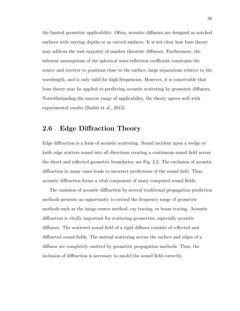
2.6 Edge Diffraction Theory
Edge diffraction is a form of acoustic scattering. Sound incident upon a wedge or
knife edge scatters sound into all directions creating a continuous sound field across
the direct and reflected geometric boundaries; see Fig. 2.2. The exclusion of acoustic
diffraction in many cases leads to incorrect predictions of the sound field. Thus,
acoustic diffraction forms a vital component of many computed sound fields.
The omission of acoustic diffraction by several traditional propagation prediction
methods presents an opportunity to extend the frequency range of geometric
methods such as the image source method, ray tracing, or beam tracing. Acoustic
diffraction is vitally important for scattering geometries, especially acoustic
diffusors. The scattered sound field of a rigid diffusor consists of reflected and
diffracted sound fields. The mutual scattering across the surface and edges of a
diffusor are completely omitted by geometric propagation methods. Thus, the
inclusion of diffraction is necessary to model the sound field correctly.

31
θ=
0
θ =θW
θ=
2θW−π−θ S
θ=θ S−π
S
(I) hFF + hGA + hD(II) hFF + hD
(III) hD
Figure 2.2: Geometric boundaries for a diffracting wedge delineate the extent of free-field radiation and geometric acoustic propagation. The angle θS − π demarcatesthe shadow boundary beyond which no free-field radiation is present. The angle2θW − π − θS demarcates the geometric boundary beyond which no geometric prop-agation is present. Three regions are defined by the geometric boundaries for thewedge geometry shown. Region (I) contains the sum of free-field radiation, geomet-ric propagation, and diffraction. Region (II) only contains free-field radiation, anddiffraction. Lastly, region (III) only contains diffraction. After (Pierce, 1974).
2.6.1 Classical Solutions of Infinite Plane/Wedge
Diffraction
Acoustic diffraction by wedges is a well studied problem, tracing back to work
conducted in the nineteenth century. The solution of plane wave acoustic diffraction
from a rigid screen is due to Sommerfeld (2004). The solution to diffraction by a
wedge was eventually generalized for a wedge of any angle (Carslaw, 1920).
Acoustic diffraction by a point source, incident upon a wedge of any angle, was
solved by MacDonald (1915). The solution of point source diffraction was later
extended to any arbitrary source type (Bromwich, 1915). The handbook solutions
for screen and wedge diffraction are based on the above developments (Bowman
et al., 1987, chs. 6 and 8). All of the solutions mentioned are for time-harmonic
sources. In contrast, the development of transient solutions of acoustic diffraction
followed time-harmonic solutions by several decades.
32
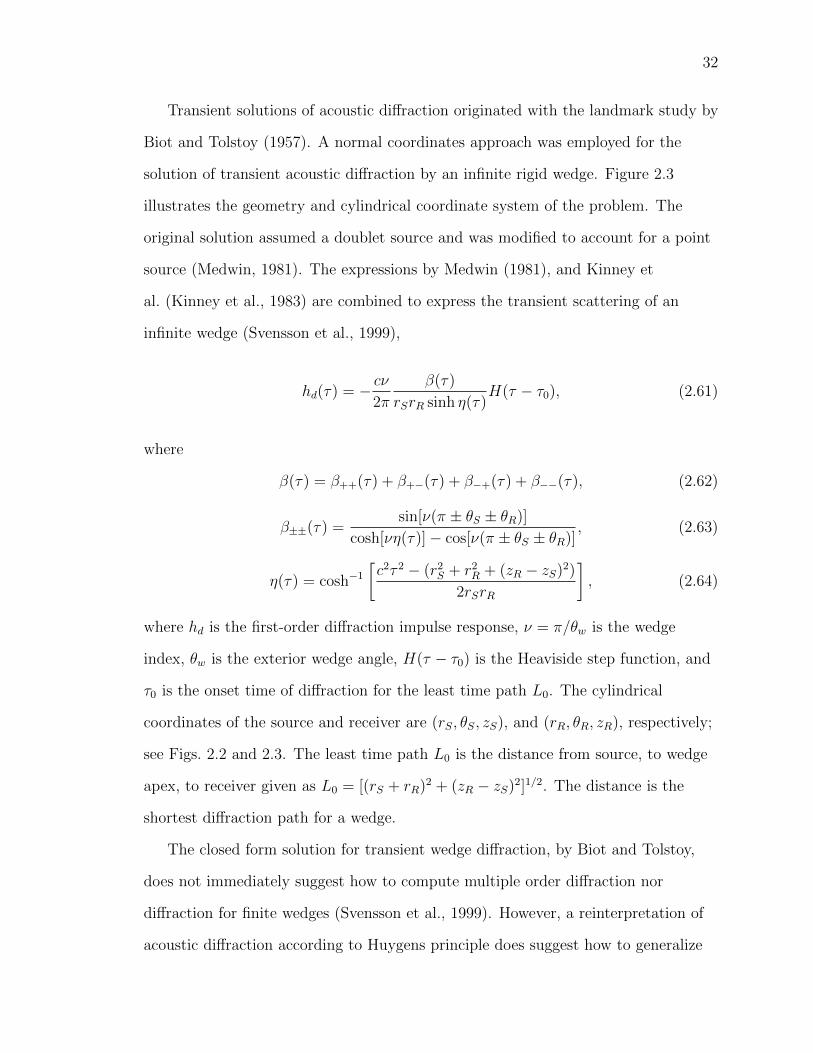
Transient solutions of acoustic diffraction originated with the landmark study by
Biot and Tolstoy (1957). A normal coordinates approach was employed for the
solution of transient acoustic diffraction by an infinite rigid wedge. Figure 2.3
illustrates the geometry and cylindrical coordinate system of the problem. The
original solution assumed a doublet source and was modified to account for a point
source (Medwin, 1981). The expressions by Medwin (1981), and Kinney et
al. (Kinney et al., 1983) are combined to express the transient scattering of an
infinite wedge (Svensson et al., 1999),
hd(τ) = − cν2π
β(τ)
rSrR sinh η(τ)H(τ − τ0), (2.61)
where
β(τ) = β++(τ) + β+−(τ) + β−+(τ) + β−−(τ), (2.62)
β±±(τ) =sin[ν(π ± θS ± θR)]
cosh[νη(τ)]− cos[ν(π ± θS ± θR)], (2.63)
η(τ) = cosh−1
[c2τ 2 − (r2
S + r2R + (zR − zS)2)
2rSrR
], (2.64)
where hd is the first-order diffraction impulse response, ν = π/θw is the wedge
index, θw is the exterior wedge angle, H(τ − τ0) is the Heaviside step function, and
τ0 is the onset time of diffraction for the least time path L0. The cylindrical
coordinates of the source and receiver are (rS, θS, zS), and (rR, θR, zR), respectively;
see Figs. 2.2 and 2.3. The least time path L0 is the distance from source, to wedge
apex, to receiver given as L0 = [(rS + rR)2 + (zR − zS)2]1/2. The distance is the
shortest diffraction path for a wedge.
The closed form solution for transient wedge diffraction, by Biot and Tolstoy,
does not immediately suggest how to compute multiple order diffraction nor
diffraction for finite wedges (Svensson et al., 1999). However, a reinterpretation of
acoustic diffraction according to Huygens principle does suggest how to generalize

33
θW
θSθR
rSrR S
R
Figure 2.3: Acoustic diffraction geometry for an infinite rigid wedge. The z-axis of thecylindrical coordinate system is aligned with the diffracting wedge, and pointing intothe page. Azimuth angles indicate the angular position of the source (θS), receiver(θR), and open wedge angle (θW ). The radial distances of the source to edge andreceiver to edge are denoted by rS, and rR, respectively. The z-coordinates (notshown) of the source and receiver are zS, and zR, respectively.
acoustic diffraction to more complex scenarios. This interpretation was shown to be
fruitful for computing the diffraction of finite wedges (Medwin, 1981), and doubly
diffracting wedges (Medwin et al., 1982). In contrast to interpreting acoustic
diffraction as propagating modes, the application of Huygens principle interprets
acoustic diffraction as the radiation of secondary sources along a wedge. This
reinterpretation laid the ground work for specifying more precisely the directivity
function of theoretical secondary sources.
2.6.2 Secondary Source Model for Finite Edge Diffraction
The basis for the secondary source model for edge diffraction begins by computing
the impulse response according to Kirchhoff’s retarded potential method (Berryhill,
1977). The pressure response for wedge diffraction is considered as a convolution
between a source signal and diffraction impulse response (Svensson et al., 1999,
34
Eq. (12)),
pd(t) = q(t) ∗ hd(t)
=
∫ ∞−∞
q(t− τ)hd(τ) dτ, (2.65)
where pd(t) is the diffracted pressure, q(t) is the source signal, and hd(t) is the
diffraction impulse response. The initial derivation by Berryhill (1977) considers a
collocated source and receiver, and the special case of a knife edge (θW = 2π). A
non-collocated source and receiver position are then considered, which are arranged
either perpendicularly or parallel to the diffracting edge. The diffraction integral is
computed as an area integration in the spatial domain. Later, the analysis is
extended and reinterpreted by Svensson et al. (1999). The starting point of the
analysis is an infinite wedge, with arbitrary wedge angle, arbitrary source position,
and arbitrary receiver position. Eq. (2.65) is cast as a convolution between the
source signal and an unknown directivity function, attenuated by the path lengths
from source to edge and edge to receiver (Svensson et al., 1999, Eq. (9))),
pd(t) =
∫ ∞−∞
q
[t− m(z) + l(z)
c
]D[α(z), γ(z), θS, θR]
m(z)l(z)dz, (2.66)
where m and l are path lengths from source to edge and edge to receiver,
respectively, and the projected angles for path lengths m and l are α and γ,
respectively; see Figs. 2.3 and 2.4. The key difference in the integral is that a line
integral is being formulated as opposed to an area integral. Conversion of the line
integral to a integration in time results in (Svensson et al., 1999, Eq. (11)),
pd(t) =
∫ ∞−∞
q(t− τ)D[α(τ), γ(τ), θS, θR]
m(τ)l(τ)
dz
dτdτ, (2.67)
35
where τ = (m(z) + l(z))/c. By mathematical analysis it is shown that the unknown
directivity function is related to Eq. (2.62) (Svensson et al., 1999, Eq. (18)),
D[α(τ), γ(τ), θS, θR] = − ν
4πβ[α(τ), γ(τ), θS, θR]. (2.68)
Substitution of Eq. (2.68) into Eq. (2.67) results in the diffracted impulse response
(Svensson et al., 1999, Eq. (19)),
hd(τ) = − ν
4π
β[α(τ), γ(τ), θS, θR]
m(τ)l(τ)
dz
dτ, (2.69)
where β is defined as Eq. (2.62) and Eq. (2.63), and η is defined as (Svensson et al.,
1999, Eq. (16)),
η(τ) = cosh−1
[1 + sinα(τ) sin γ(τ)
cosα(τ) cos γ(τ)
]. (2.70)
Note, Eq. (2.69) is the continuous-time expression for finite wedge diffraction.
Solution of the diffraction impulse response is based on a line integral along the
diffracting edge. Parameters derived for the Biot and Tolstoy solution are
determined to satisfy the unknown directivity function. The second order diffraction
impulse response, for a truncated wedge, is derived following the same procedure of
retarded potentials. It is shown the second order diffracted impulse response is a
scaled first order diffraction impulse from the secondary sources along the first edge
to the receiver, via the second edge. The scaling is based on a sum of directivity
functions with respect to the first and second edge (Svensson et al., 1999, Fig. (4)
and Eq. (27)).
2.6.3 Solution of Diffraction Singularities
The closed form solutions for diffraction impulse responses contain two types of
singularities. The first singularity occurs at the onset time of diffraction, τ0. It is
36
z
L0 mu
lu
ml
llzS
zR
zA
zu
zl
αu
γu
−αl
−γl
S
R
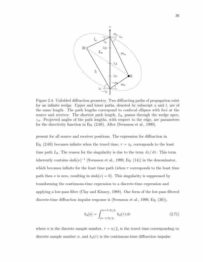
Figure 2.4: Unfolded diffraction geometry. Two diffracting paths of propagation existfor an infinite wedge. Upper and lower paths, denoted by subscript u and l, are ofthe same length. The path lengths correspond to confocal ellipses with foci at thesource and receiver. The shortest path length, L0, passes through the wedge apex,zA. Projected angles of the path lengths, with respect to the edge, are parametersfor the directivity function in Eq. (2.68). After (Svensson et al., 1999).
present for all source and receiver positions. The expression for diffraction in
Eq. (2.69) becomes infinite when the travel time, τ = τ0, corresponds to the least
time path L0. The reason for the singularity is due to the term dz/ dτ . This term
inherently contains sinh(ν)−1 (Svensson et al., 1999, Eq. (14)) in the denominator,
which becomes infinite for the least time path (when τ corresponds to the least time
path then ν is zero, resulting in sinh(ν) = 0). This singularity is suppressed by
transforming the continuous-time expression to a discrete-time expression and
applying a low-pass filter (Clay and Kinney, 1988). One form of the low-pass filtered
discrete-time diffraction impulse response is (Svensson et al., 1999, Eq. (30)),
hd[n] =
∫ (n+1/2)/fs
(n−1/2)/fs
hd(τ) dτ (2.71)
where n is the discrete sample number, τ = n/fs is the travel time corresponding to
discrete sample number n, and hd(τ) is the continuous-time diffraction impulse
37
response as in Eq. (2.69). The integration effectively acts as a low-pass filter. To
decrease the attenuation by low-pass filtering, it was suggested to integrate over a
time window of 4/fs (Clay and Kinney, 1988); however, increasing the sampling
frequency achieves a similar reduction in attenuation. The second singularity arises
when the receiver is along a geometric acoustic boundary at the onset time of
diffraction. Two geometric boundaries exist: the shadow boundary and reflection
boundary; see Fig. 2.2. When the receiver is located on the shadow boundary or
reflection boundary, the expression for β becomes infinite. The term cosh[νη(τ)] is
equal to one at the onset time of diffraction. For a receiver on a geometric boundary
the term cos[ν(π ± θS ± θR) is equal to one. Thus, the denominator of β is zero at
the onset time of diffraction for a receiver on a geometric boundary; see Eqs. (2.63)
and (2.64). This singularity exists in order to account for the discontinuity of the
geometric acoustic field. An analytic approximation, which suppresses the
singularity, bounds the diffraction impulse response (Svensson and Calamia, 2006).
The form of the approximation is,
β[α(z), γ(z), θS, θR]
m(z)l(z)≈ B0
(z2rel +B1)(z2
rel +B2zrel +B3), (2.72)
where zrel = z − zA is the z-coordinate relative to the wedge apex, see Fig. 2.4. The
variables B0 through B4 are defined as,
B0 =4L2
0ρ3 sin[ν(π ± θS ± θR)]
ν2(1 + ρ4)[(1 + ρ)2 sin2 ψ − 2ρ],
B1 =4L2
0ρ2 sin2[ν(π ± θS ± θR)/2]
ν2(1 + ρ)4,
B2 = − 2L0(1− ρ)ρ cosψ
(1 + ρ)[(1 + ρ)2 sin2 ψ − 2ρ],
B3 =2L2
0ρ2
(1 + ρ)2[(1 + ρ)2 sin2 ψ − 2ρ]. (2.73)

38
The dimensionless variable ρ = rR/rS is the ratio of radial receiver distance and
source distance, and ψ is the projected angle of the least time path with the wedge
defined implicitly as,
tanψ =rS + rRzR − zS
. (2.74)
The approximation in Eq. (2.72) facilitates the numerical computation of wedge
diffraction when either the receiver is on the reflection or shadow boundaries and
the time sample closely corresponds to the onset time of diffraction. Special care is
required for the exact limits of integration over the time sample corresponding to
the onset of diffraction (cf. Eq. (2.71)). The simplest case requires the upper limit of
integration to be the extent of the first sample. Other considerations are provided in
(Svensson and Calamia, 2006).
2.6.4 Discrete-time Diffraction Formulation
Numerical computation of first, second, and higher order diffraction are achieved by
numerically integrating the continuous-time impulse response, as in Eq. (2.71).
Transformation of the variable of integration, in Eq. (2.71), from time to a
differential element along the wedge allows the integration to be conducted as a line
integral. Distinct diffraction contributions are approximated by the midpoint of two
coordinates corresponding to the starting and ending times for one time sample. For
example, first order diffraction is determined by a simple midpoint approximation to
the integral of the continuous-time impulse response as (Svensson et al., 1999,
Eq. (34)),
hd(n) ≈ − ν
4π
β[α(zn), γ(zn), θS, θR]
m(zn)l(zn)∆zn, (2.75)
where zn is the midpoint coordinate of zn2 and zn1, which corresponds to discrete
times τ = (n± 1/2)/(fs), and ∆zn is the edge element width (zn2− zn1). Setting the
length of each edge element width to a constant, ∆z, results in determining the ith
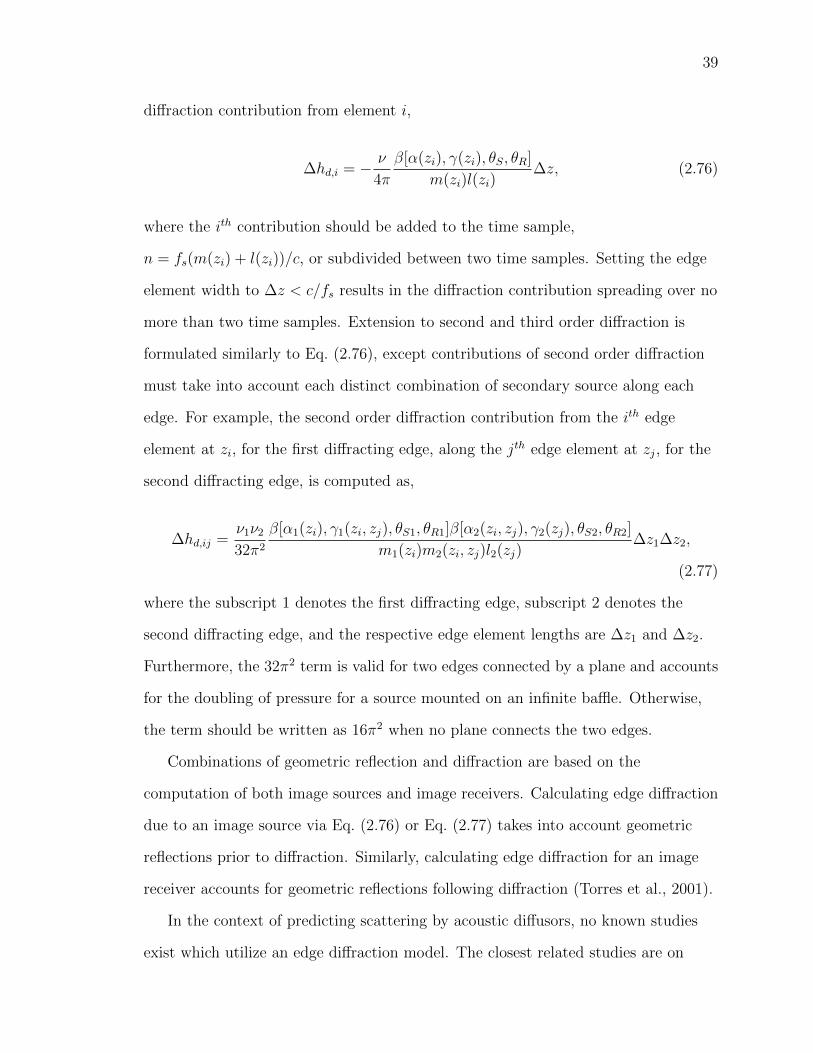
39
diffraction contribution from element i,
∆hd,i = − ν
4π
β[α(zi), γ(zi), θS, θR]
m(zi)l(zi)∆z, (2.76)
where the ith contribution should be added to the time sample,
n = fs(m(zi) + l(zi))/c, or subdivided between two time samples. Setting the edge
element width to ∆z < c/fs results in the diffraction contribution spreading over no
more than two time samples. Extension to second and third order diffraction is
formulated similarly to Eq. (2.76), except contributions of second order diffraction
must take into account each distinct combination of secondary source along each
edge. For example, the second order diffraction contribution from the ith edge
element at zi, for the first diffracting edge, along the jth edge element at zj, for the
second diffracting edge, is computed as,
∆hd,ij =ν1ν2
32π2
β[α1(zi), γ1(zi, zj), θS1, θR1]β[α2(zi, zj), γ2(zj), θS2, θR2]
m1(zi)m2(zi, zj)l2(zj)∆z1∆z2,
(2.77)
where the subscript 1 denotes the first diffracting edge, subscript 2 denotes the
second diffracting edge, and the respective edge element lengths are ∆z1 and ∆z2.
Furthermore, the 32π2 term is valid for two edges connected by a plane and accounts
for the doubling of pressure for a source mounted on an infinite baffle. Otherwise,
the term should be written as 16π2 when no plane connects the two edges.
Combinations of geometric reflection and diffraction are based on the
computation of both image sources and image receivers. Calculating edge diffraction
due to an image source via Eq. (2.76) or Eq. (2.77) takes into account geometric
reflections prior to diffraction. Similarly, calculating edge diffraction for an image
receiver accounts for geometric reflections following diffraction (Torres et al., 2001).
In the context of predicting scattering by acoustic diffusors, no known studies
exist which utilize an edge diffraction model. The closest related studies are on

40
surface roughness (Kinney et al., 1983; Novarini and Medwin, 1985). Possible
reasons for the lack of studies include the limited geometric generality, the
increasing complexity of higher-order diffraction, and an incompatibility with most
geometric propagation methods. In spite of the limited geometric generality of edge
diffraction models the wedge shape was shown to approximate a sinusoidal surface
fairly well (Novarini and Medwin, 1985). A second difficulty is the computational
bottleneck for computing higher orders of diffraction. Consider two edges, with the
same length, that are subdivided into N edge elements. For second-order diffraction
N2 diffraction contributions must be computed. A potential solution to this
difficulty is an integral equation formulation for higher-order diffraction (Asheim
and Svensson, 2013). Another challenge for edge diffraction models are the present
incompatibilities with most geometric propagation models. Studies on edge
diffraction using image sources (Torres et al., 2001) or ray tracing (Antani et al.,
2012) demonstrate an inherent incompatibility between the two models. It is
suggested that adaptive beam tracing is a compatible technique, which is considered
in Chapter 4.
2.7 Summary
The theoretical foundations for scattering prediction methods are discussed at length
for wave-based methods, and analytic models. Wave-based methods, especially the
BEM, have found widespread use in the prediction of acoustic diffusor scattering.
The future trend is to compute the transient scattering characteristics with either
the time-domain BEM or FDTD. Alternatively, analytic models offer the potential
for faster computations at the expense of geometric generality. For example the
dimensionality of edge scattering is reduced to a line integral as opposed to a
surface or volume integration. The potential for computing transient scattering by

41
edge diffraction and adaptive beam tracing is explored in Chapters 4 and 5.

Chapter 3
Adaptive Tetrahedral Tracing
Adaptive tetrahedral tracing is an advanced image source method. As a geometric
propagation method it shares many similarities with other techniques such as the
image source method (Allen and Berkley, 1979), ray tracing (Kulowski, 1985), and
classical beam tracing (Lewers, 1993). However, several features distinguish the
method from those mentioned previously. The primary distinction is the conceptual
view of sound propagation: free-field radiation of sound is a set of expanding
tetrahedrons and geometric reflection is a larger set of expanding tetrahedral
frustums. The initial set of tetrahedrons generally increases upon reflection due to
tetrahedral subdivision. For example, as an initial tetrahedron expands in volume,
intersecting with the geometric domain, portions of the tetrahedron split according
to the incident geometry. Being most closely related to adaptive beam tracing
(Campo et al., 2000; Drumm and Lam, 2000; Stephenson, 1996) the adaptive
tetrahedral algorithm presented in this chapter expands upon previous work by
defining the algorithm as clearly as possible and proposing alternative strategies
when appropriate.
This chapter details the adaptive tetrahedral tracing algorithm. Section 3.1
presents related past work on beam tracing for acoustics, including non-adaptive and
42

43
adaptive techniques. Theoretical and algorithmic details of the adaptive tetrahedral
tracing method are given in Section 3.2, and a summary is given in Section 3.3.
3.1 Prior Work
Beam tracing first developed as a method for computer graphics applications
(Heckbert and Hanrahan, 1984; Dadoun et al., 1985). The geometric coherence of
beam tracing was found to be a superior method for generating computer images as
opposed to ray tracing. In the context of computer graphics, geometric coherence is
the conceptual treatment of continuous light propagation as opposed to discrete
light propagation, as in ray tracing. For example, a propagating beam may be
thought of as an infinite bundle of rays as opposed to discrete rays. Applications of
beam tracing to acoustic modeling started emerging in the following decades. A
number of different beam tracing models have been developed that are both
non-adaptive and adaptive.
A non-adaptive beam tracing model was combined with a radiant exchange
model to simulate the decay response of a space (Lewers, 1993). The non-adaptive
beam tracing algorithm developed by Lewers was supplemented by a radiant
exchange model in order to predict the late energy decay within a space. Another
implementation examined the effect of multilayer boundaries within an enclosure
(Wareing and Hodgson, 2005). More recently a non-adaptive beam tracing model
was applied to study the effects of modeling enclosure boundaries as either an
impedance boundary or an energy absorption boundary (Jeong, 2012).
The first study on adaptive beam tracing outlined a rough algorithmic
description (Stephenson, 1996). However, no results based on the algorithm were
provided in the study. An adaptive beam tracing model combined with binary space
partitioning was developed for real-time auralization purposes (Funkhouser et al.,

44
2004). This implementation is distinguished from non-adaptive beam tracing
models by including a model for diffraction: the uniform theory of diffraction
(UTD) (Kouyoumjian and Pathak, 1974). Another adaptive beam tracing model
approximates the reflection of propagating beams by omitting portions of the
incident beam after beam subdivision, which is supposedly balanced by distributing
the acoustic energy across the reflected beams (Campo et al., 2000). In the study by
Campo et al. (2000) diffraction is treated by Maekawa’s noise barrier model
(Maekawa, 1968) for room acoustic predictions. Lastly, an adaptive beam tracing
model was combined with a radiosity method for the purpose of computing the
energy decay of rooms (Drumm and Lam, 2000). Unlike other adaptive beam
tracing models the study by Drumm and Lam (2000) omits diffraction effects.
There are several inherent drawbacks for classical beam tracing algorithms.
First, the reliance upon a central vector for determining the propagation paths of a
beam does not account for a beam incident upon two or more polygons (Campo
et al., 2000). As a result specular paths of propagation are incorrectly detected or
missed leading to an incorrect computation of the geometric acoustic field; see
Fig. 3.1(a). In a related manner ray tracing results in acoustic aliasing since the
domain is spatially sampled by a finite number of rays (Lehnert, 1993). The
solution for this first issue is to clip or subdivide beams that intersect multiple
polygons (Drumm and Lam, 2000). A second drawback inherent in both classical
and adaptive beam tracing is a second form of acoustic aliasing, which occurs when
the cross-section of a propagating beam becomes larger than a polygon; see
Fig. 3.1(b). A simple approach to resolve the second issue is to refine the initial
beam density. Lastly, accounting for acoustic diffraction in classical beam tracing is
beset by the same difficulties associated with ray tracing. Typically, a ray does not
exactly intersect a diffracting edge, so edge detection becomes a difficulty. Heuristic
extensions of diffraction formulas based on quantum mechanics and the use of edge
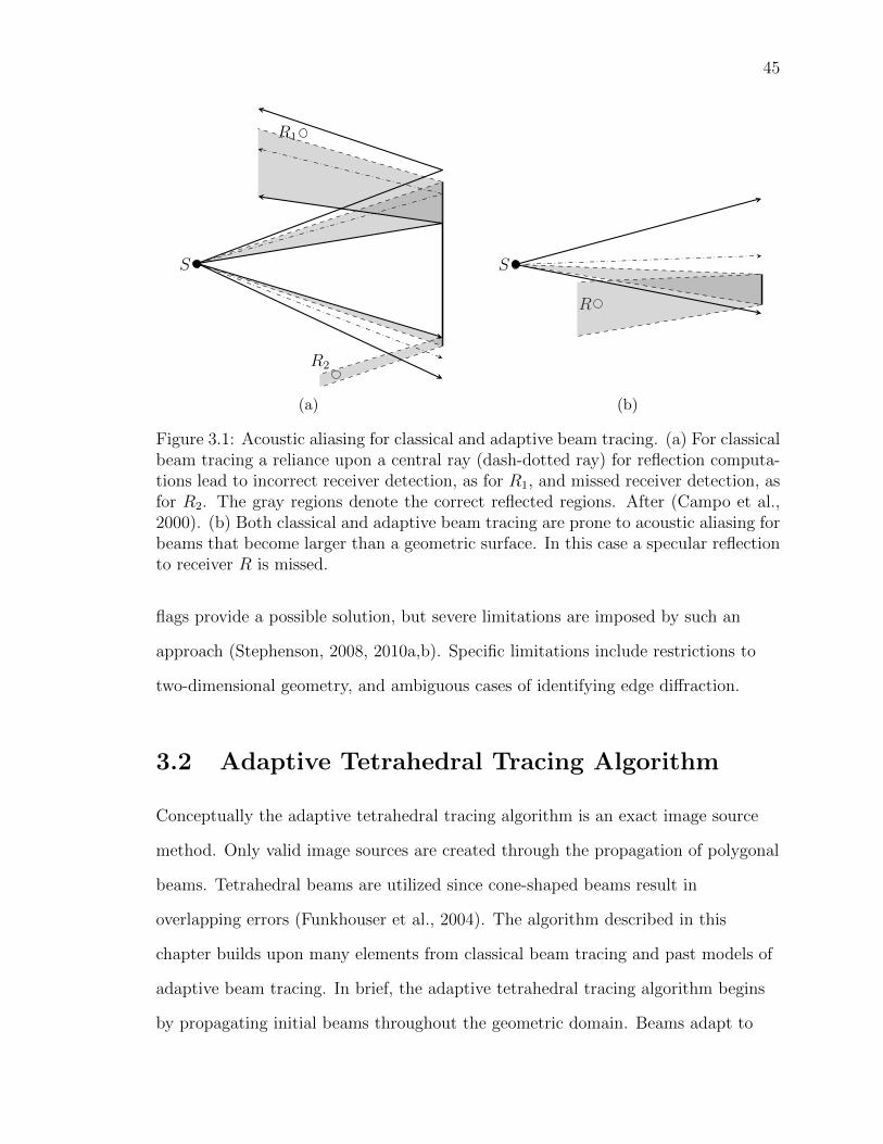
45
S
R1
R2
(a)
S
R
(b)
Figure 3.1: Acoustic aliasing for classical and adaptive beam tracing. (a) For classicalbeam tracing a reliance upon a central ray (dash-dotted ray) for reflection computa-tions lead to incorrect receiver detection, as for R1, and missed receiver detection, asfor R2. The gray regions denote the correct reflected regions. After (Campo et al.,2000). (b) Both classical and adaptive beam tracing are prone to acoustic aliasing forbeams that become larger than a geometric surface. In this case a specular reflectionto receiver R is missed.
flags provide a possible solution, but severe limitations are imposed by such an
approach (Stephenson, 2008, 2010a,b). Specific limitations include restrictions to
two-dimensional geometry, and ambiguous cases of identifying edge diffraction.
3.2 Adaptive Tetrahedral Tracing Algorithm
Conceptually the adaptive tetrahedral tracing algorithm is an exact image source
method. Only valid image sources are created through the propagation of polygonal
beams. Tetrahedral beams are utilized since cone-shaped beams result in
overlapping errors (Funkhouser et al., 2004). The algorithm described in this
chapter builds upon many elements from classical beam tracing and past models of
adaptive beam tracing. In brief, the adaptive tetrahedral tracing algorithm begins
by propagating initial beams throughout the geometric domain. Beams adapt to

46
occluding geometry through beam clipping operations. Ray tracing techniques are
utilized for beam clipping (Drumm and Lam, 2000). For sufficiently complex
geometry beam clipping may operate recursively. Geometric details are resolved by
the recursive process resulting in subdivided beam mappings of all ensonified
regions. Clipped beam profiles, which are not triangular, are subdivided into
triangular regions by a constrained Delaunay triangulation (Yvinec, 2013). Finally,
the image source location corresponding to each subdivided triangular beam profile
is calculated and new tetrahedral beams are reflected throughout the domain.
3.2.1 Surface Geometry
The surface geometry is defined within a Cartesian coordinate system. Polygons are
geometric elements that compose the geometric domain. In this study each polygon
is a quadrilateral with four vertices, ~v1 to ~v4, and four edge vectors, ~e1 to ~e4, see
Fig. 3.2. A vertex is defined as a three-dimensional coordinate, eg. ~v1 = (x1, y1, z1).
Each edge vector is defined as (O’Rourke, 1998, p. 1),
~ei = ~vi mod 4+1 − ~vi for i = 1, 2, 3, 4, (3.1)
where mod is the modulus operator. In the composition of a geometric domain
hanging vertices are disallowed, or equivalently adjacent polygons only share
common vertices. A hanging vertex is a vertex of a polygon that lies on the edge of
another polygon. The unit normal of a polygon is defined as,
n =~e1 × ~e2
|~e1 × ~e2|, (3.2)
where n is the unit normal, the operator × is the cross product, and | · | is the norm
of the vector. A polygon unit normal is oriented such that the normal points away
from the “front” of a polygon. Each polygon is associated with a plane that is

47
xy
z
~r
~r ′
~r − ~r ′n
Π
~v1
~v2
~v3
~v4
~e1
~e2
~e3
~e4
Figure 3.2: Geometric definitions for a polygon. The polygon, Π, is associated witha plane. The position vector ~r ′ is a known point on the plane and all points on theplane, ~r, satisfy Eq. (3.3). The polygon is defined by four vertices, ~v1 to ~v4, and fouredge vectors, ~e1 to ~e4. The direction of the polygon unit normal, n is governed by theright-hand rule, applied to the cyclic ordering of vertices.
mathematically defined as (Long, 2006, p. 789),
n · (~r − ~r ′) = 0, (3.3)
where the operator · is the dot product of two vectors, ~r ′ is the position vector of a
known point on the plane, and ~r is a position vector to points in the plane
associated with the polygon Π. Equation (3.3) concisely defines all the points on the
plane associated with the polygon Π. The equation stipulates that the dot product
between the plane unit normal, n, and the vector ~r − ~r ′ must be identically zero for
~r corresponding to points in the plane, see Fig. 3.2.
Expansion of Eq. (3.3) results in another form for the plane equation,
nx(x− x′) + ny(y − y′) + nz(z − z′) = 0, (3.4)

48
where the unit normal is defined in terms of Cartesian components,
n = nxi+ ny j + nzk, and similarly for the position vectors. Algebraic rearrangement
of Eq. (3.4) results in an alternative plane equation,
ax+ by + cz + d = 0, (3.5)
where a, b, and c are the respective vector components of the unit normal vector n.
The perpendicular distance from the plane to the origin is given as d = −n · ~r ′.
In order to facilitate the storage of geometric information, matrices are utilized.
A vertex matrix stores each unique vertex in a K by three matrix where K is the
total number of vertices and each column corresponds to a Cartesian coordinate.
Polygons are specified as a combination of four vertex references in a L by four
matrix where L is the total number of polygons and each entry is a vertex reference
to the corresponding row in the vertices matrix. Vertices are ordered according to
the right hand rule, which dictates the direction of the polygon unit normal. The
polygons at the boundaries of the domain have outward pointing normals. Polygon
unit normals are in a L by three matrix with each column corresponding to a
component of the normal. All the edge vectors are stored in a 4L by four matrix.
Each row corresponds to a particular edge vector. The first column references a
specific polygon and the last three columns are the edge vector components. Lastly,
every polygon is defined as either acoustically rigid or anechoic in a column vector
with length L. Acoustically rigid polygons are associated with a numerical value of
zero and anechoic polygons are associated with a numerical value of one.
3.2.2 Omnidirectional Source
An icosahedron is a geometric primitive that has found common use in beam
tracing for modeling an omnidirectional source. The vertices of an icosahedron,

49
centered at the origin, are defined as (Drumm and Lam, 2000),
(0,±1,±τ),
(±1,±τ, 0), (3.6)
(±τ, 0,±1),
where τ = (1 +√
5)/2 is the golden ratio; see Fig. 3.3(a). The vertices of the
icosahedron are normalized to the unit sphere and serve as unit vectors for beam
rays; see Eq. (3.7). Other geometric primitives exist for a source definition, but the
selection of an icosahedron is motivated by the fact that each face contains equal
cross sectional areas. As such, computations based on intensity or the assignment of
source directivity are easily facilitated.
In order to resolve detailed geometries, it is necessary to subdivide the
cross-sectional areas of the source. Beginning with an icosahedron primitive, the
faces of the icosahedron are subdivided in order to increase the density of
propagating beams. Subdivision is achieved by bisecting the edges of each
icosahedron face (Loop, 1987), projecting all of the resultant vertices to the unit
sphere, and finally determining the convex hull of all vertices (Pion and Teillaud,
2013). This method is known as Loop subdivision. See Fig. 3.3(b) for an illustration
of an icosahedron source refined twice by Loop subdivision.
3.2.3 Beam Definition
A beam is comprised of three beam rays, three beam planes, and three beam plane
unit normals. A matrix with Q rows and three columns stores each beam reference.
Each row corresponds to a beam and the entries in each row reference the beam
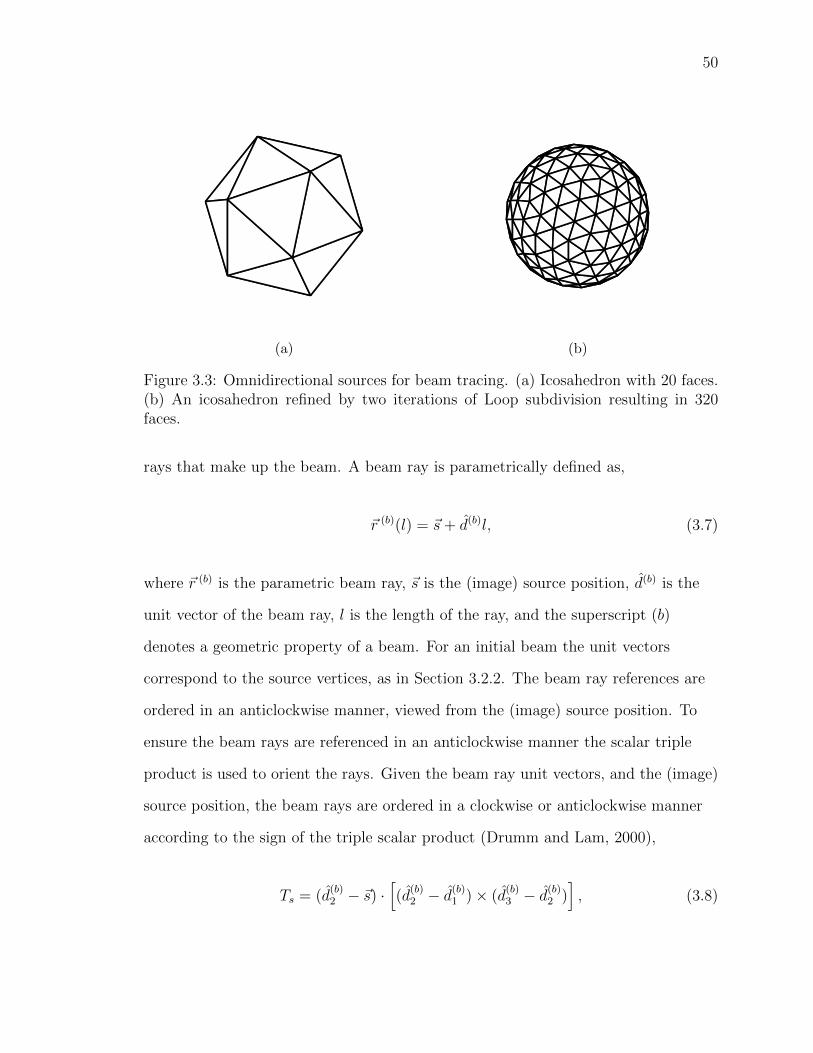
50
(a) (b)
Figure 3.3: Omnidirectional sources for beam tracing. (a) Icosahedron with 20 faces.(b) An icosahedron refined by two iterations of Loop subdivision resulting in 320faces.
rays that make up the beam. A beam ray is parametrically defined as,
~r (b)(l) = ~s+ d(b)l, (3.7)
where ~r (b) is the parametric beam ray, ~s is the (image) source position, d(b) is the
unit vector of the beam ray, l is the length of the ray, and the superscript (b)
denotes a geometric property of a beam. For an initial beam the unit vectors
correspond to the source vertices, as in Section 3.2.2. The beam ray references are
ordered in an anticlockwise manner, viewed from the (image) source position. To
ensure the beam rays are referenced in an anticlockwise manner the scalar triple
product is used to orient the rays. Given the beam ray unit vectors, and the (image)
source position, the beam rays are ordered in a clockwise or anticlockwise manner
according to the sign of the triple scalar product (Drumm and Lam, 2000),
Ts = (d(b)2 − ~s) ·
[(d
(b)2 − d
(b)1 )× (d
(b)3 − d
(b)2 )], (3.8)

51
where d(b)1 to d
(b)3 are the beam ray unit vectors for one beam, Ts > 0 indicates a
clockwise orientation (viewed from the source), and Ts < 0 an anticlockwise
orientation. The beam rays are ordered in an anti-clockwise manner so that the
beam plane unit normals point out of the beam (Lewers, 1993). The beam plane
unit normals are computed as,
n(b)i =
d(b)i × d
(b)i mod 3+1
|d(b)i × d
(b)i mod 3+1|
for i = 1, 2, 3. (3.9)
The beam plane normals are stored in a P by three matrix where each column is a
Cartesian component of the beam plane normal. Conceptually a beam is a
tetrahedron that expands in volume with a stationary vertex, being the source or
image source position (Lewers, 1993). Three bounding planes, Π(b)1 , Π
(b)2 , and Π
(b)3
are beam planes which delimit the volume of the beam. The plane equation for each
beam plane is defined by the beam plane normal, from Eq. (3.7), and the beam
origin, cf. Eq. (3.3). Three bounding beam rays, ~r(b)1 , ~r
(b)2 , and ~r
(b)3 define the extent
of the beam; see Fig. 3.4.
3.2.4 Beam Propagation
A beam is bounded by three beam rays that define the extent of the beam. In
contrast to classical beam tracing, which relies upon a central ray, the adaptive
tetrahedral tracing algorithm utilizes each beam ray to determine the full extent of
a beam. The added complexity is balanced by the ability to identify multiple
polygons intersected by a beam (Lewers, 1993). Alternatively, a central ray can only
identify a single polygon intersection. The fundamental geometric principles that
govern the extent of rays applies equally to beam rays.
The first step to computing the extent of a beam ray is to determine the length
of the ray to the nearest polygon. Substituting Eq. (3.7) into the plane equation,

52
~r(b)1
~r(b)2
~r(b)3
Π(b)1
Π(b)2
Π(b)3
Figure 3.4: A representative beam originating from an icosahedron source. Threebeam planes, Π
(b)1 , Π
(b)2 , and Π
(b)3 delimit the volume of the beam. Associated with
each beam plane is a beam plane unit normal that points out of the beam (not shown),
defined by Eq. (3.9). Three beam rays, ~r(b)1 , ~r
(b)2 , and ~r
(b)3 define the extent of the
beam.
Eq. (3.3), and let the known point on the plane be a vertex of the polygon, Π,
n · (~r (b)(l)− ~v) = 0, (3.10)
where ~v is any one of the four vertices of the polygon Π, and n is the polygon
normal. Expanding Eq. (3.10) and rearranging terms results in the length of the
beam ray (Long, 2006),
n · (~s+ d(b)l − ~v) = 0, (3.11)
l =n · (~v − ~s)n · d(b)
. (3.12)
It must be stressed that this beam ray length is the length of the ray to the plane
associated with the polygon Π. It does not necessarily mean the ray intersects Π.
For multiple polygons the ray length computed by Eq. (3.12) is ambiguous since

53
not every ray length corresponds to a polygon intersection. Multiple tests are
applied to confirm which polygon is the nearest polygon intersected by a beam ray.
First, the ray length to a plane, associated with a polygon, must be for a potentially
visible polygon. A simple test on potential visibility is based on the dot product of
the beam ray unit vector and a polygon normal,
d(b) · n > 0, (3.13)
which indicates the unit normal and the unit vector point into the same half-space.
Once the set of polygons is reduced by Eq. (3.13), all the ray lengths are computed
for the reduced set of polygons. Beam propagation is physically constrained for
positive ray lengths. Thus, negative ray lengths are excluded from consideration.
Finally, a point-in-polygon test is conducted. Several algorithms exist for checking
whether a point is within a polygon, but the most computationally efficient
algorithm relies upon the Jordan curve theorem (Long, 2006, p. 790). The algorithm
is known as the ray-crossing algorithm (O’Rourke, 1998, sec. 7.5). The algorithm is
applied to each polygon associated with a positive ray length in ascending order.
The first polygon which satisfies the point-in-polygon test is the intersected
polygon. The intersected polygon is linked to the beam ray. If a beam ray intersects
two or more polygons at a polygon edge or vertex, then a list is generated that links
the beam ray with references to each intersected polygon. Initial beam rays are
shown for a beam in Fig. 3.5.
3.2.5 Ensonification Mapping
Once the length of each respective beam ray is computed then the ensonified region
is mapped. Ensonified regions are demarcated by illumination rays. Illumination
rays are traced along the intersection between a beam plane, and a polygon or

54
Figure 3.5: Initial propagation of beam rays. The icosahedron source is refined onceand the beam rays are indicated by red rays.
multiple polygons. An initial illumination ray begins from the endpoint of one beam
ray and ultimately continues until the next beam ray end point. The illumination
ray traces a path within the beam plane and along polygons. Once an illumination
ray intersects another beam ray endpoint, then another illumination ray is traced
along the following beam plane. The process repeats until an enclosed area of
ensonification is determined.
The ray equation for an illumination ray depends upon a beam plane and the
polygon intersected by a beam ray or illumination ray. The intersection of a beam
plane and the polygon depend upon the unit normals of the beam plane and
polygon. The unit normal for a beam plane is determined by Eq. (3.9) and the unit
normal for a polygon is determined by Eq. (3.2). Computation of the unit vector for
the initial illumination ray is based on the cross product of the beam plane normal
and polygon normal (Drumm and Lam, 2000),
d(il) = n(b) × n, (3.14)
55
where d(il) is the unit vector for the illumination ray. The superscript (il) indicates
a property of an illumination ray. The unit vector computed by Eq. (3.14) is
collinear with the line of intersection between the beam plane and the plane
associated with the intersected polygon.
It is possible for a beam ray to intersect two or more polygons; see Sec. 3.2.4. It
was suggested by Drumm and Lam (2000) that when an illumination ray intersects
a polygon vertex, the correct unit vector, originating from the vertex, is the one
that makes the sharpest turn at the vertex relative to the prior illumination ray.
This criteria is closely related to determining the initial unit vector originating from
a beam ray end point on a polygon edge or vertex. Computation of the angle
between two vectors is facilitated by the dot product. For example, consider the dot
product of two unit vectors of subsequent illumination rays,
d(il)i · d
(il)i−1 = |d(il)
i ||d(il)i−1| cos(θ), (3.15)
where the subscripts i and i− 1 indicates two connected illumination rays in the
same beam, and θ is the angle formed between the two unit vectors in
three-dimensional space. This criteria may be sufficient to determine a subsequent
unit vector; however it is insufficient to determine the initial unit vector for a beam
ray intersecting a polygon vertex or edge. The criteria sufficient to handle both
cases is based upon a physical argument. An illumination ray that originates from a
polygon edge or vertex must continue within another polygon. Concisely, this can
be stated as the principle of continuation. Infinitesimal rays are generated from the
point of intersection with unit vectors computed according to Eq. (3.14). A
point-in-polygon query is conducted for each infinitesimal ray end point and the
associated polygon. The ray that continues within another polygon contains the
correct unit vector.

56
Once the correct unit vector for an initial illumination ray is determined then an
illumination ray, or multiple illumination rays, are traced to the following beam ray
end point. The ray length to another beam plane or polygon is determined by
Eq. (3.12). The correct length of an illumination ray is based upon the minimum
distance to another polygon or beam plane. If the ray length to a beam plane is
equal to or less than the length to the nearest polygon, then the length to the beam
plane is selected and a beam plane intersection is noted. Otherwise, if the ray
length to the nearest polygon is less than the length to the nearest beam plane, then
the length to the polygon is selected and a polygon intersection is noted. For a
beam plane intersection, or a polygon intersection, several cases require special
attention. The nature of the intersection is evaluated for the purpose of continuing
or terminating the ensonification mapping along a beam plane.
If a beam plane is intersected one of three cases are applicable. The first case
applies when an illumination ray intersects a beam plane, and the end point of the
ray coincides with the following beam ray end point. If this case applies, then the
ensonification mapping within the current beam plane is terminated, and
ensonification mapping continues along the next beam plane starting at the last
intersection point (following beam ray end point). A second case occurs when a
beam plane is intersected and the illumination ray end point does not coincide with
the following beam ray end point. This case applies when an illumination ray
traverses into a region of space invisible to the (image) source. In this particular
case a reverse ensonification mapping is conducted. The current beam plane normal
is reversed, and an illumination ray is generated from the following beam ray end
point. This procedure effectively traces illumination rays in a reversed sense along
the current beam plane. While a reverse trace is being conducted, each new
illumination ray is checked against an overlapping condition with existing
illumination rays. If an overlap occurs, then the intersection of the two illumination
57
rays is computed, the overlapped ray is eliminated, and the illumination ray tracing
continues along the following beam plane. The third case occurs for reflected beams.
A scenario may arise such that an illumination ray intersects a polygon and a beam
plane. Furthermore, the intersection point is on the following beam ray. In this case
the illumination ray tracing is terminated in the current beam plane and continues
along the next beam plane, starting from the following beam ray end point.
If a polygon is intersected, then the next unit vector is determined according to
one of two cases. Before defining the treatment of the two cases, it is necessary to
define the terms locally concave and locally convex points. For example, the wedge
geometry in Fig. 2.3 shows an open wedge angle for a convex wedge since the open
wedge angle is greater than 180. A point on the edge of the wedge is locally
convex. In contrast, a concave wedge is a wedge with an open wedge angle less than
180. Thus, a point on the edge of the wedge is locally concave. If an illumination
ray intersects a polygon, then the intersection point is locally convex or locally
concave depending upon the orientation of the intersected polygon at the point.
However, an intersection point that coincides with three or more polygons may lead
to some ambiguity in classifying the local geometry. Assuming that no ambiguity of
the intersection point exists, the first case is an illumination ray intersecting a
polygon, or multiple polygons, at a locally concave wedge. The following
illumination ray is computed according to Eq. (3.14) and the principle of
continuation. The second case is the intersection of a locally convex wedge. The
visibility of the intersected polygon(s) is/are checked by Eq. (3.13). If the polygons
are visible, then the principle of continuation is employed. Otherwise, discontinuous
illumination ray tracing is employed. Discontinuous illumination ray tracing is the
process of displacing the start point of the following illumination ray. The displaced
start point is computed similarly to the end point of a beam ray, as in Sec. 3.2.4.
Conceptually, a ray originates from the (image) source point, extends beyond the
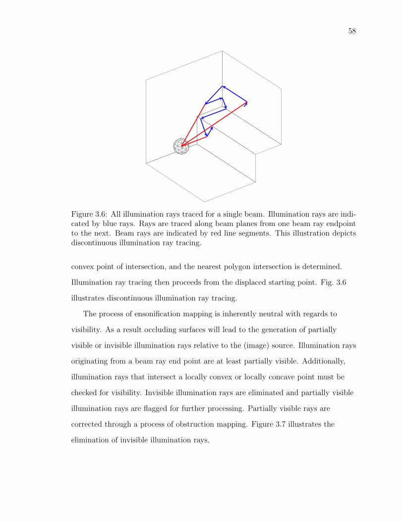
58
Figure 3.6: All illumination rays traced for a single beam. Illumination rays are indi-cated by blue rays. Rays are traced along beam planes from one beam ray endpointto the next. Beam rays are indicated by red line segments. This illustration depictsdiscontinuous illumination ray tracing.
convex point of intersection, and the nearest polygon intersection is determined.
Illumination ray tracing then proceeds from the displaced starting point. Fig. 3.6
illustrates discontinuous illumination ray tracing.
The process of ensonification mapping is inherently neutral with regards to
visibility. As a result occluding surfaces will lead to the generation of partially
visible or invisible illumination rays relative to the (image) source. Illumination rays
originating from a beam ray end point are at least partially visible. Additionally,
illumination rays that intersect a locally convex or locally concave point must be
checked for visibility. Invisible illumination rays are eliminated and partially visible
illumination rays are flagged for further processing. Partially visible rays are
corrected through a process of obstruction mapping. Figure 3.7 illustrates the
elimination of invisible illumination rays.

59
Figure 3.7: Elimination of illumination rays not visible to the source. Illuminationrays are indicated by blue line segments and beam rays are indicated by red linesegments. Two invisible illumination rays are eliminated within the beam, compareto Fig. 3.6.
3.2.6 Occlusion Mapping
Acoustic shadowing results from occluding geometry. Mapping the ensonification
region in the presence of occluding geometry requires special attention. Drumm and
Lam (2000) offer vague suggestions for occlusion mapping. In contrast, Campo et
al. (2000) describe a more complete description for occlusion mapping, but as the
study admits several scenarios are not mapped exactly. Thus, the algorithm
sketched below offers a more comprehensive treatment of occlusion mapping.
Mapping the shadowing geometry profiles the occlusion and projects the profile
to the furthest reaches of the incident beam. As part of the ensonification mapping
procedure, an indication of occluding geometry is noted when an illumination ray
intersects a polygon at a locally convex point. A locally convex point indicates the
possibility that some geometric feature is occluding a portion of the beam.
Confirmation of an occluding feature is dependent upon the convex point satisfying

60
a grazing incidence condition. The condition of grazing incidence is satisfied if one
or more polygons at the convex vertex or edge is not visible to the (image) source.
Once grazing incidence is confirmed at a locally convex point then an edge finding
algorithm proceeds to find the shadowing edges contained within the beam. Every
connected edge is determined by a breadth-first search (Cormen et al., 2009), and
pushed onto a first-in first-out stack. Simultaneously the profile of each edge is
projected to the furthest extent of the incident beam through a procedure similar to
illumination ray tracing; see Section 3.2.5.
While the stack containing the shadowing edges is not empty. the extent of a
shadowing edge is determined. The result is a shadow edge ray. It is determined
whether a shadow edge ray intersects a polygon, multiple polygons, or a beam
plane. If a shadow edge ray intersects a beam plane, and is completely visible, then
shadow beam rays are generated from the (image) source through the end points of
the shadow edge ray. The intersection points of the shadow beam rays serve as the
starting and ending points for shadow illumination ray tracing. The shadow
illumination rays are traced from one shadow beam ray end point to the other
through the same process as illumination ray tracing, refer to Sec. 3.2.5. If another
locally convex point is intersected while tracing a shadow illumination ray, then the
occlusion mapping procedure is recursively conducted. Once any recursive
procedures have completed then the shadow edge is pushed off the stack. An
alternative scenario is when a shadow edge ray intersects a polygon, or multiple
polygons. If the intersection point is locally convex, then the same procedure for
shadow illumination ray tracing is conducted as above. Afterwards the shadowing
edge is pushed off the stack. If the intersection point satisfies the condition of
grazing incidence, then adjacent shadowing edges are determined. Otherwise, if the
intersection point is locally concave, then the procedure is treated as a beam plane
intersection. The process of occlusion mapping continues until the shadow edge

61
Figure 3.8: Shadow illumination rays are traced for an occluding edge. A shadowedge ray, shown as a green ray, is computed, which intersects a beam plane. Twoshadow beam rays, shown as violet rays, project the end points of the shadow edgeray to the furthest extent within the beam. The shadow illumination rays, shown asteal rays, are traced from one shadow beam ray intersection point to the other. Theillumination rays are shown as blue line segments.
stack is empty. An example of occlusion mapping is shown in Fig. 3.8.
3.2.7 Ensonification Mapping Corrections
Shadow illumination rays facilitate mapping corrections of illumination rays.
Shadow illumination rays demarcate the termination of partially visible illumination
rays. A procedure to correct the length of illumination rays must take two cases
into account. Either the length of a ray must be modified, or the origin of the ray
must be moved and the length modified. In both cases the necessary computations
involve computing ray intersections.
The mechanics of determining ray intersections rely upon comparing unit
directional vectors. All origin and end points of shadow illumination rays are
computed for a particular beam. For each partially visible illumination ray the

62
Figure 3.9: Illumination rays, shown as blue line segments, are trimmed accordingto the location of shadow illumination rays, shown as teal line segments. In thisparticular case one illumination ray is trimmed, compare to Fig. 3.7.
visible point of the ray is determined. Unit directional vectors from the visible point
to each origin/end point of all other shadow rays are compared to the unit
directional vector of the illumination ray. If a matching unit directional vector is
found then the length of the illumination ray is matched to the length of the vector
from the visible point to the origin/end point of the shadow illumination ray.
Alternatively, if a match for a reversed unit directional vector is found then the
origin of the illumination ray is redefined to be the origin/end point of the shadow
ray, and the length of the illumination is adjusted accordingly. Figure 3.9 illustrates
one illumination ray trimmed. Compare to Fig. 3.8.
Edge rays are computed from locally concave intersection points by illumination
rays or shadow illumination rays. An edge finding algorithm, described in Sec. 3.2.6,
is utilized to determine all the edge rays originating from a concave junction that
are visible within the beam. As Fig. 3.10 illustrates an edge ray goes beyond the
region of visibility. Generally, edge rays are traced until another polygon or beam

63
Figure 3.10: Edge rays are traced from concave junctions. One edge ray is shown asa magenta line segment.
plane is intersected. In the case of Fig. 3.10 the vertical edge ray traces from the
concave junction to a beam plane. A ray trimming procedure is conducted on all
edge rays, similar to illumination rays.
The total ensonification mapping concludes by gathering all illumination rays,
shadow illumination rays, shadow edge rays, and edge rays together. Once all
trimming corrections are conducted the total mapping for the ensonified region is
complete. The conglomeration of all corrected rays are hereafter referred to as
ensonification rays. Fig. 3.11 shows all regions of ensonification for a single beam. It
is clear that relying upon a central ray for beam propagation is far from accurate
considering the effect of shadowing.
3.2.8 Subdivision of Ensonification Mapping
Once an ensonification mapping is completed it may become necessary to subdivide
the ensonification regions into coplanar, triangular, regions. Maintaining tetrahedral
beam propagation requires the subdivision of non-triangular ensonification regions

64
Figure 3.11: Ensonification rays define the extent of direct or reflected acoustic prop-agation from the source. The ensonification rays shown as blue line segments
into triangular regions. For ensonification regions that map across several polygons
the regions must be subdivided into unique coplanar groupings of ensonification
rays. Furthermore, each grouping must form a simple closed polygon. For example,
Fig. 3.11 illustrates three unique coplanar groupings of ensonification rays. Once
each unique coplanar region is identified then the non-triangular regions are
subdivided according to a constrained Delaunay triangulation (Yvinec, 2013).
The first challenge for the subdivision of ensonified regions is to determine which
ensonification rays are coplanar and form a simple closed polygon. Assuming all the
ensonification rays in a beam are unique the first step is to determine which
ensonification rays are coplanar. A naive approach is enumerate all triplet
combinations of ensonification rays. For a small number of rays this approach is
satisfactory; however, as the number of rays increases the number of combinations
increases very rapidly since the total number of enumerations is equivalent to the
binomial coefficient, (n
k
)=
n!
(n− k)!k!, (3.16)
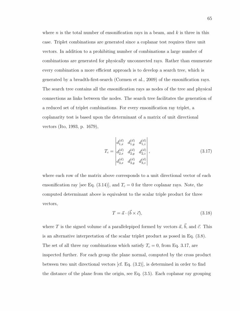
65
where n is the total number of ensonification rays in a beam, and k is three in this
case. Triplet combinations are generated since a coplanar test requires three unit
vectors. In addition to a prohibiting number of combinations a large number of
combinations are generated for physically unconnected rays. Rather than enumerate
every combination a more efficient approach is to develop a search tree, which is
generated by a breadth-first-search (Cormen et al., 2009) of the ensonification rays.
The search tree contains all the ensonification rays as nodes of the tree and physical
connections as links between the nodes. The search tree facilitates the generation of
a reduced set of triplet combinations. For every ensonification ray triplet, a
coplanarity test is based upon the determinant of a matrix of unit directional
vectors (Ito, 1993, p. 1679),
Tc =
∣∣∣∣∣∣∣∣∣∣d
(il)1,x d
(il)1,y d
(il)1,z
d(il)2,x d
(il)2,y d
(il)2,z
d(il)3,x d
(il)3,y d
(il)3,z
∣∣∣∣∣∣∣∣∣∣, (3.17)
where each row of the matrix above corresponds to a unit directional vector of each
ensonification ray [see Eq. (3.14)], and Tc = 0 for three coplanar rays. Note, the
computed determinant above is equivalent to the scalar triple product for three
vectors,
T = ~a · (~b× ~c), (3.18)
where T is the signed volume of a parallelepiped formed by vectors ~a, ~b, and ~c. This
is an alternative interpretation of the scalar triplet product as posed in Eq. (3.8).
The set of all three ray combinations which satisfy Tc = 0, from Eq. 3.17, are
inspected further. For each group the plane normal, computed by the cross product
between two unit directional vectors [cf. Eq. (3.2)], is determined in order to find
the distance of the plane from the origin, see Eq. (3.5). Each coplanar ray grouping

66
with the same plane normal, and distance from the origin are consolidated further.
Set operations are performed on the ray groupings to consolidate the rays that
satisfy coplanarity, and connectedness.
For each unique ensonification region, a simple closed polygon is formed and
non-triangular regions are subdivided according to a constrained Delaunay
triangulation. The formation of a simple closed polygon requires the ensonification
rays to be arranged in a cyclic manner (O’Rourke, 1998, pp. 1, 2). Generally
ensonification rays are not arranged in a cyclic manner since they are composed of
illumination rays, shadow illumination rays, and edge rays. Thus, it becomes
necessary to reverse the orientation of rays accordingly. Once all the ensonification
rays form a simple closed polygon, the rays are projected to a Cartesian plane. The
projection plane is dependent upon the largest component of the plane normal.
Whichever component of the normal is largest the plane of projection is the plane
formed by the two other Cartesian components. For example, if the component of
the normal is largest along the y-axis then the plane of projection is the x-z plane.
Constraints for the Delaunay triangulation are specified by an ordered list of
ensonification ray origins, which confines the ensonification region. Finally, a
constrained Delaunay triangulation is conducted on the ordered vertices, resulting
in triangular regions of ensonification; see Fig. 3.12.
3.2.9 Child Beam Generation
If the ensonification mapping includes multiple regions requiring subdivision, then
multiple child beams are generated for reflection. Otherwise, for a single triangular
region the tetrahedral profile of the beam is preserved for reflection. Each child
beam is generated by creating beam rays that originate from the (image) source to
the vertices of a triangular region. The beam rays are oriented in an anticlockwise
manner with the aid of the triple scalar product, cf. Eq. (3.8). Beam plane normals

67
Figure 3.12: Subdivision of ensonification mapping. A coplanar, connected, region ishighlighted by blue line segments. Constrained Delaunay triangulation of the regionresults in triangular regions, denoted by the blue dashed line.
are computed by Eq. (3.9). The intersection points of each beam ray are noted for
each child beam, and any beam ray intersecting multiple polygons is noted as in
Sec. 3.2.4. A child beam generated by the process of adaptive tetrahedral tracing is
shown in Fig. 3.13. In the presence of occluding geometry a tetrahedral beam is
clipped according to the extent of the occlusion. The clipping process results in the
generation of several new beams. Greater computational resources are required for
the adaptive beam tracing process compared to the ray tracing method, but in
comparison to the image source method, less resources are required for high
reflection orders (Drumm and Lam, 2000). However, in contrast to the ray tracing
method or the image source method, the adaptive beam tracing method accurately
determines the visibility of diffracting wedges from the (image) source.

68
Figure 3.13: A child beam is generated for a portion of an ensonified region. Theensonified region is subdivided into two triangular regions by a constrained Delaunaytriangulation. One child beam is shown in orange.
3.2.10 Beam Reflection
Each tetrahedral beam generated by the process in Sections 3.2.3–3.2.9 is either
reflected or anechoically absorbed, assuming that all surfaces are either acoustically
rigid or anechoic. The reflection of tetrahedral beams is governed by the geometric
law of reflection. The geometric law of reflection states that the angle of incidence is
equal to the angle of reflection. Equivalently, by the method of images the reflecting
ray is determined by creating an image source, which is a mirrored source position
about the reflecting point. The image source for a propagating beam is computed as
(Drumm, 2005),
~s (i) = ~s+ 2[(d(b)l) · n]n, (3.19)
where d(b)l is the vector associated with a beam ray of a tetrahedral beam, ~s (i) is
the the image source position, and n is the unit normal of the polygon intersected
by the beam ray. Similarly the reflected unit vectors of each beam ray are computed
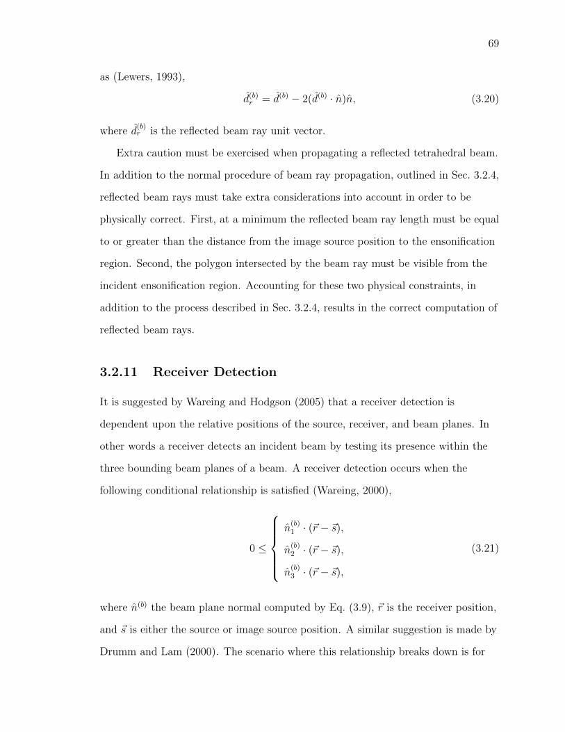
69
as (Lewers, 1993),
d(b)r = d(b) − 2(d(b) · n)n, (3.20)
where d(b)r is the reflected beam ray unit vector.
Extra caution must be exercised when propagating a reflected tetrahedral beam.
In addition to the normal procedure of beam ray propagation, outlined in Sec. 3.2.4,
reflected beam rays must take extra considerations into account in order to be
physically correct. First, at a minimum the reflected beam ray length must be equal
to or greater than the distance from the image source position to the ensonification
region. Second, the polygon intersected by the beam ray must be visible from the
incident ensonification region. Accounting for these two physical constraints, in
addition to the process described in Sec. 3.2.4, results in the correct computation of
reflected beam rays.
3.2.11 Receiver Detection
It is suggested by Wareing and Hodgson (2005) that a receiver detection is
dependent upon the relative positions of the source, receiver, and beam planes. In
other words a receiver detects an incident beam by testing its presence within the
three bounding beam planes of a beam. A receiver detection occurs when the
following conditional relationship is satisfied (Wareing, 2000),
0 ≤
n
(b)1 · (~r − ~s),
n(b)2 · (~r − ~s),
n(b)3 · (~r − ~s),
(3.21)
where n(b) the beam plane normal computed by Eq. (3.9), ~r is the receiver position,
and ~s is either the source or image source position. A similar suggestion is made by
Drumm and Lam (2000). The scenario where this relationship breaks down is for

70
non-concave geometric domains. Coupled spaces is one particular example. A
receiver may be within the volume of the bounding beam planes, but not within the
extent of the beam. A stricter test is based on a different geometric test.
Since every propagating beam is a tetrahedral beam, a geometric query is
sufficient to determine if a receiver detects an incident beam. Hence, a
point-in-tetrahedron query determines whether a propagating beam intersects a
point receiver. The test is based on the Cartesian coordinates of the tetrahedron and
receiver. Five determinants are computed for the query (Yamaguchi, 2002, p. 221),
d0 =
∣∣∣∣∣∣∣∣∣∣∣∣∣
t1,x t1,y t1,z 1
t2,x t2,y t2,z 1
t3,x t3,y t3,z 1
sx sy sz 1
∣∣∣∣∣∣∣∣∣∣∣∣∣, (3.22)
d1 =
∣∣∣∣∣∣∣∣∣∣∣∣∣
rx ry rz 1
t2,x t2,y t2,z 1
t3,x t3,y t3,z 1
sx sy sz 1
∣∣∣∣∣∣∣∣∣∣∣∣∣, (3.23)
d2 =
∣∣∣∣∣∣∣∣∣∣∣∣∣
t1,x t1,y t1,z 1
rx ry rz 1
t3,x t3,y t3,z 1
sx sy sz 1
∣∣∣∣∣∣∣∣∣∣∣∣∣, (3.24)
d3 =
∣∣∣∣∣∣∣∣∣∣∣∣∣
t1,x t1,y t1,z 1
t2,x t2,y t2,z 1
rx ry rz 1
sx sy sz 1
∣∣∣∣∣∣∣∣∣∣∣∣∣, (3.25)
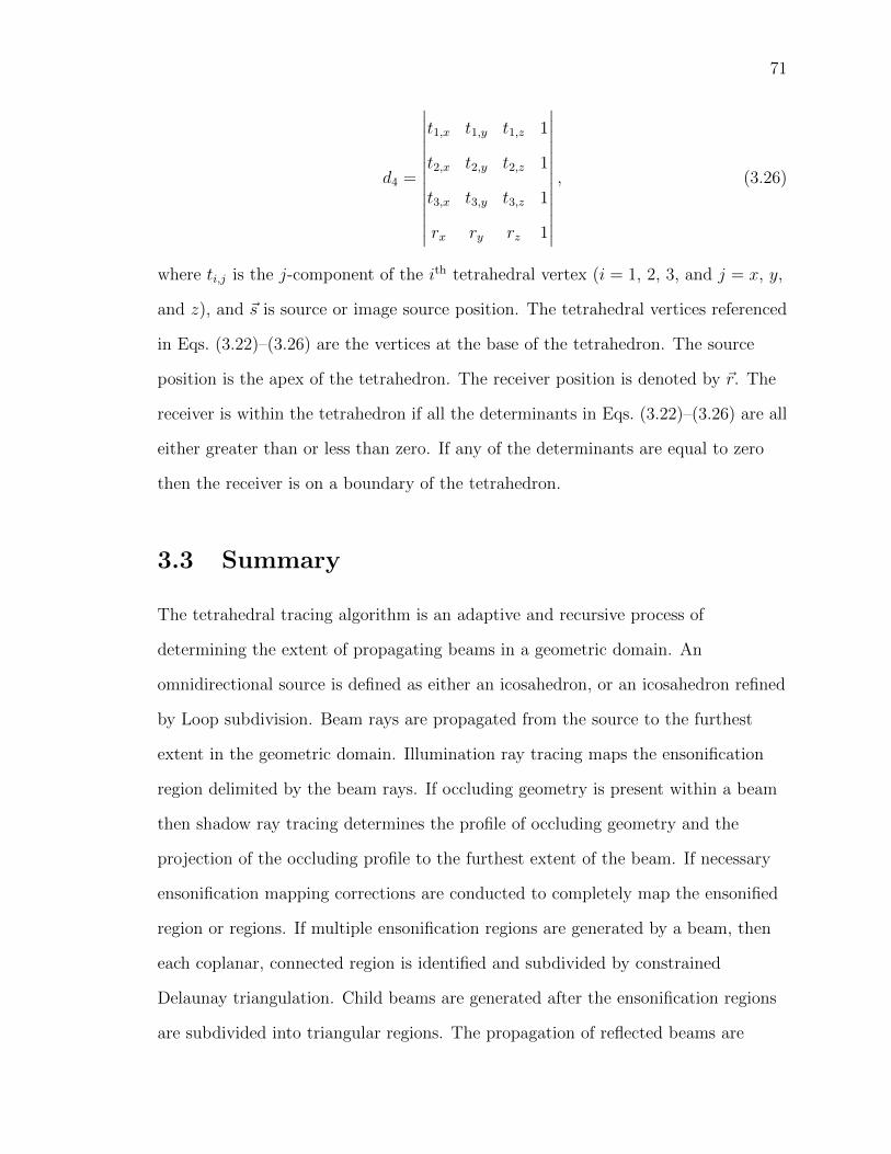
71
d4 =
∣∣∣∣∣∣∣∣∣∣∣∣∣
t1,x t1,y t1,z 1
t2,x t2,y t2,z 1
t3,x t3,y t3,z 1
rx ry rz 1
∣∣∣∣∣∣∣∣∣∣∣∣∣, (3.26)
where ti,j is the j-component of the ith tetrahedral vertex (i = 1, 2, 3, and j = x, y,
and z), and ~s is source or image source position. The tetrahedral vertices referenced
in Eqs. (3.22)–(3.26) are the vertices at the base of the tetrahedron. The source
position is the apex of the tetrahedron. The receiver position is denoted by ~r. The
receiver is within the tetrahedron if all the determinants in Eqs. (3.22)–(3.26) are all
either greater than or less than zero. If any of the determinants are equal to zero
then the receiver is on a boundary of the tetrahedron.
3.3 Summary
The tetrahedral tracing algorithm is an adaptive and recursive process of
determining the extent of propagating beams in a geometric domain. An
omnidirectional source is defined as either an icosahedron, or an icosahedron refined
by Loop subdivision. Beam rays are propagated from the source to the furthest
extent in the geometric domain. Illumination ray tracing maps the ensonification
region delimited by the beam rays. If occluding geometry is present within a beam
then shadow ray tracing determines the profile of occluding geometry and the
projection of the occluding profile to the furthest extent of the beam. If necessary
ensonification mapping corrections are conducted to completely map the ensonified
region or regions. If multiple ensonification regions are generated by a beam, then
each coplanar, connected region is identified and subdivided by constrained
Delaunay triangulation. Child beams are generated after the ensonification regions
are subdivided into triangular regions. The propagation of reflected beams are

72
governed by the geometric law of reflection. Finally, receiver detection is based on a
point-in-tetrahedron query, which eliminates false-positive detections past strategies
employed.
One particular advantage the adaptive tetrahedral tracing algorithm has
compared to other geometric methods is the identification of diffracting edges. This
capability is utilized to link together the algorithm with a secondary source model
for edge diffraction; see Secs. 2.6.2–2.6.4. Details on joining the two models of
acoustic propagation are given in Ch. 4.

Chapter 4
Fusion of Adaptive Tetrahedral
Tracing and Edge Diffraction
Scattering by rigid acoustic diffusors is a combination of geometric propagation and
diffraction. The multitude of interactions include reflections, diffractions, and
permutations of the two mechanisms. Wave-based prediction methods, outlined in
Chapter 2, solve for the scattered field as the sum total of all permutations of
reflections and diffraction. The identification of individual propagation mechanisms
is not possible due to the mathematical formulation. In contrast, an edge diffraction
model accounts for specific, identifiable diffraction events; see Sec. 2.6. Similarly, a
geometric propagation method accounts for specific, identifiable reflection
contributions. The two models taken alone are insufficient to characterize diffusor
scattering; however, linking the two offers an alternative approach for time-domain
prediction.
In contrast to image source methods or ray tracing methods, adaptive
tetrahedral tracing is highly compatible with edge scattering models. The adaptive
tetrahedral tracing algorithm, described in Chapter 3, precisely maps the incident
and reflected sound fields. In the presence of geometric discontinuities the mapping
73

74
is generated by splitting incident and reflected beams. The same geometric
discontinuities that lead to beam splitting may also lead to acoustic diffraction. By
design the acoustic mapping generated by adaptive tetrahedral tracing inherently
contains information required for edge diffraction computations. Therefore, by
extracting the information required for edge diffraction computations from the
acoustic mapping, a bridge is formed between adaptive tetrahedral tracing and edge
scattering models.
The chapter proceeds by exploring the link between adaptive tetrahedral tracing
and an edge diffraction model in Sec. 4.1. After, in Sec. 4.2 graph theory is applied
to the generation of geometric reflection and diffraction permutations. Sec. 4.3
details the generation of digital impulse responses from scattering predictions. The
joint model for acoustic scattering is numerically verified by three case studies in
Sec. 4.4. Finally, a summary is given in Sec. 4.5.
4.1 Linking Adaptive Tetrahedral Tracing and
Edge Diffraction
The adaptive tetrahedral tracing method generates an acoustic mapping of incident
and reflected sound fields. The incident and reflected sound fields are determined by
propagating tetrahedral beams from the source or image sources. In the presence of
surface discontinuities a propagating tetrahedral beam is split, conforming to the
incident geometry. The conforming nature of adaptive tetrahedral tracing is the key
element for identifying diffracting edges.
If a tetrahedral beam is split, then portions of split profiles may be collinear
with surface discontinuities. For each child beam, new beam rays are computed
from the (image) source to the triangular profile, as in Sec. 3.2.4. At a surface
discontinuity a beam ray intersects two or more polygons. If two or more beam rays

75
of a child beam intersect multiple polygons, then a diffracting edge may be collinear
with a portion of the beam profile. The condition of collinearity is satisfied if two
polygon unit normals, associated with one beam ray, match two other polygon unit
normals, associated with another beam ray.
Once a diffracting edge is identified the wedge geometry is deduced from the
available information. First, the z-axis of a cylindrical coordinate system is aligned
with the edge. The direction of the axis is opposite to the edge vector of the
reference polygon. More precisely, the reference polygon contains a unit normal in
the opposite direction of the azimuth unit vector. In other words, the fingers of a
right hand come out of the reference polygon when the thumb is aligned with the
z-axis of the wedge. Once the reference polygon is established then the open wedge
angle is computed with the aid of the triple scalar product,
Ts = −k · (n1 × n2), (4.1)
where k is the unit vector aligned with the z-axis, n1 is the reference polygon unit
normal, n2 is the second polygon forming the wedge, and Ts is the triple scalar
product. The computation of the open wedge angle depends upon the sign of the
triple scalar product,
θW =
π − arccos(n1 · n2) if Ts < 0,
arccos(n1 · n2) + π if Ts > 0,
(4.2)
where θW is the open wedge angle computed in radians. If the open wedge angle is
any angle equal to π/m radians, where m is an integer, then no acoustic diffraction
is emitted from the wedge (Biot and Tolstoy, 1957). After the open wedge angle is
computed, the length of the diffracting wedge is determined by the distance between
the two beam ray end points. Finally, the cylindrical coordinates of the (image)

76
source and (image) receiver are computed relative to the wedge by two coordinate
transformations. The global Cartesian coordinate system is mapped to a local
Cartesian coordinate system along the wedge. The local coordinate system is
oriented such that the x-axis points into the reference polygon, and the y-axis
points away from the reference polygon unit normal. The local Cartesian
coordinates are then transformed to cylindrical coordinates.
The extraction of wedge parameters from an acoustic mapping of sound
propagation links together adaptive tetrahedral tracing and edge diffraction models.
Specifically, a secondary source model for edge diffraction, described in Sec. 2.6, is
well-suited for computing first-order, second-order, and higher-order diffraction in
the time-domain. The wedge parameters generated by the extraction process are
sufficient for the computation of first-order diffraction impulse responses. However,
additional considerations are required for second, and higher-order diffraction.
4.2 Graph Theory Applied to Multiple-Order
Diffraction
Determination of sound propagation paths from source, to multiple edges, and then
to a receiver is essentially a problem associated with graph theory (Bang-Jensen and
Gutin, 2001). The problem is similar to finding sound transmission paths in
statistical energy analysis (Guasch and Cortes, 2009). Given the source, edges, and
receiver are considered as nodes in a directed graph it becomes essential to
determine which paths are valid; see Fig. 4.1(a). A defining feature of a directed
graph for sound propagation is the one-way sound transmission from source to all
visible edges. Furthermore, all edges visible to the receiver result in sound
diffraction directed to the receiver. Sound transmission is bidirectional between
edges, if a portion of one edge is visible to another. Construction of the directed

77
12
34
56
7
S
R
(a)
S
12
3
4
56
7
R
(b)
Figure 4.1: Directed graph representation of source, edges, and receiver. (a) Physicalgeometry of source, scattering object, and receiver. Each diffracting edge of the objectis labeled numerically. (b) Directed graph indicating paths of sound propagation fromsource to receiver, and source to edges to receiver.
graph, for sound propagation, is based on visibility. Visibility between a source to
an edge, an edge to another edge, and an edge to a receiver is necessary for
diffraction sound propagation. Source to edge, or receiver to edge visibility is
determined by the adaptive beam tracing algorithm. By tracing beams from either
the source or receiver, visible edges are identified by the beam clipping and
subdivision process; see Ch. 3. On the other hand, edge to edge visibility is a
distinct challenge since it requires computing region to region visibility, rather than
point to region visibility. Several different approaches exist to determine edge to
edge visibility (Cohen-Or et al., 2003). The following discussion is limited to two
different approaches for determining edge to edge visibility.
Various methods exist for determining edge to edge visibility, ranging from the
simple to very complex. A simplistic manner of determining edge to edge visibility
is based upon a ray casting technique from each edge midpoint; refer to Sec. 3.2.4.
If no obstructions exist between each edge midpoint, then the edges are considered
visible. A more accurate method is based on computing conservative from-region
visibility between edges to identify all possible mutually diffracting edges (Antani
et al., 2012). After the conservative from-region visibility computation each

78
diffracting edge is subdivided into equal sized segments. Ray casting between each
segment midpoint is conducted in order to determine the mutual visibility of edge
segments. Unobstructed rays between each segment midpoint indicates a visible
edge segment. Visible edge to edge segments give second order diffraction
contributions as in Eq. 2.77. The first approach based upon ray-casting from an
edge midpoint to another edge midpoint is used for visibility testing in the present
study in order to avoid time-consuming computations for from-region visibility, as in
(Antani et al., 2012). A further simplification is to assume each mutually visible
edge is completely visible. Thus, no account is taken of partially visible edges for
second- and higher-order diffraction. This assumption is justifiable when computing
two-dimensional acoustic diffusors since the diffracting edges have a consistent
profile in two-dimensions. Once visibility computations are completed then the
relationships between the source, edges, and receiver are established as a directed
graph; see Fig. 4.1(b). In the directed graph representation the source, diffracting
edges, and receiver are treated as nodes. The sound transmission paths between the
source, edges, and receiver are denoted as directed edges or links in the directed
graph. The computational equivalent of the directed graph is the adjacency matrix.
The adjacency matrix is a graph theoretic data structure which defines the
relationships between nodes of a directed graph (Bang-Jensen and Gutin, 2001,
p. 30). Each entry of the adjacency matrix is either a zero or a one. A entry of one
in the ith row and jth column of the matrix indicates a directed link between the
nodes i and j. The adjacency matrix, formed by edge to edge visibility, is a subset
of the complete adjacency matrix. Provided the source to edge visibility and edge to
receiver visibility information are known, the full adjacency matrix is formed by
including edge to edge visibility. The analog of the adjacency matrix is an incidence
list, which is also known as an adjacency list representation (Bang-Jensen and
Gutin, 2001, p. 30). An incidence list is formed from the adjacency matrix in order
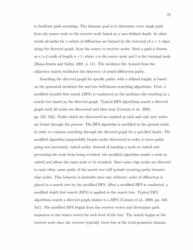
79
to facilitate path searching. The ultimate goal is to determine every single path
from the source node to the receiver node based on a user-defined depth. In other
words all paths for n orders of diffraction are formed by the traversal of n+ 1 edges
along the directed graph, from the source to receiver nodes. Such a path is known
as a (s,t)-walk of length n+ 1, where s is the source node and t is the terminal node
(Bang-Jensen and Gutin, 2001, p. 11). The incidence list, formed from the
adjacency matrix facilitates the discovery of sound diffraction paths.
Searching the directed graph for specific paths, with a defined length, is based
on the generated incidence list and two well-known searching algorithms. First, a
modified breadth first search (BFS) is conducted on the incidence list resulting in a
search tree based on the directed graph. Typical BFS algorithms search a directed
graph until all nodes are discovered and then stop (Cormen et al., 2009,
pp. 531–534). Nodes which are discovered are marked as such and only new nodes
are found through the process. The BFS algorithm is modified in the present study
in order to continue searching through the directed graph for a specified depth. The
modified algorithm purposefully forgets nodes discovered in order to trace paths
going over previously visited nodes. Instead of marking a node as visited and
preventing the node from being revisited, the modified algorithm marks a node as
visited and allows the same node to be revisited. Since some edge nodes are directed
to each other, some paths of the search tree will include recurring paths between
edge nodes. This behavior is desirable since any arbitrary order of diffraction is
placed in a search tree by the modified BFS. After a modified BFS is conducted, a
modified depth first search (DFS) is applied to the search tree. Typical DFS
algorithms search a directed graph similar to a BFS (Cormen et al., 2009, pp. 540,
541). The modified DFS begins from the receiver vertex and determines path
sequences to the source vertex for each level of the tree. The search begins at the
receiver node since the receiver typically views less of the total geometric domain
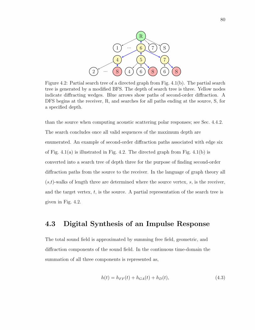
80
R
6...1 7 S
54 7
S...2 64 S 6 S
Figure 4.2: Partial search tree of a directed graph from Fig. 4.1(b). The partial searchtree is generated by a modified BFS. The depth of search tree is three. Yellow nodesindicate diffracting wedges. Blue arrows show paths of second-order diffraction. ADFS begins at the receiver, R, and searches for all paths ending at the source, S, fora specified depth.
than the source when computing acoustic scattering polar responses; see Sec. 4.4.2.
The search concludes once all valid sequences of the maximum depth are
enumerated. An example of second-order diffraction paths associated with edge six
of Fig. 4.1(a) is illustrated in Fig. 4.2. The directed graph from Fig. 4.1(b) is
converted into a search tree of depth three for the purpose of finding second-order
diffraction paths from the source to the receiver. In the language of graph theory all
(s,t)-walks of length three are determined where the source vertex, s, is the receiver,
and the target vertex, t, is the source. A partial representation of the search tree is
given in Fig. 4.2.
4.3 Digital Synthesis of an Impulse Response
The total sound field is approximated by summing free field, geometric, and
diffraction components of the sound field. In the continuous time-domain the
summation of all three components is represented as,
h(t) = hFF (t) + hGA(t) + hD(t), (4.3)

81
where hFF (t) is the free field impulse response, hGA(t) is the geometric impulse
response, and hD(t) is the diffraction impulse response. The summation of acoustic
components is valid for linear acoustics. The free field and geometric sound fields
are determined directly by the beam tracing algorithm; see Ch. 3. The free field
impulse response is simply a scaled Dirac delta function,
hFF (t) =δ(t−R0/c)
R0
, (4.4)
where δ is the Dirac delta function, and R0 is the distance from the source to
receiver. Specular reflection is accounted for by determining image source
contributions,
hGA(t) =N∑n=1
δ(t−Rn/c)
Rn
, (4.5)
where Rn are the distances from image sources to receiver and N is the total
number of image sources. Note, Eq. (4.5) implies acoustically rigid boundary
conditions for reflecting surfaces. The diffraction sound field is approximated by
summing a finite number of diffraction contributions by the secondary source model
for edge diffraction (see Section 2.6),
hD(t) =K∑i=1
hD,i(t), (4.6)
where K is the total number of diffraction permutations.
Acoustic scattering by diffusors is approximated by Eq. (4.3) where Eq. (4.6) is
the approximating term. Since scattering by diffusors is limited to a finite number
of reflections Eq. (4.4) satisfies the geometric field exactly. However, a finite-number
of diffraction permutations is accounted for in Eq. (4.6). For example, in the present
study, permutations include any number of geometric reflections proceeding or
succeeding diffraction. However, geometric reflections between diffraction events are

82
not accounted for. An extra layer of complexity is required for computing geometric
reflections between diffraction events. Image, or mirrored, edges must be computed
for determining such permutations. Additionally, slope diffraction is neglected
(Summers, 2013) and a finite order of diffraction is computed.
The numerical computation of Eq. (4.3) is synthesized digitally by converting
the continuous-time expressions to discrete-time expressions. The Dirac delta
function in Eqs. (4.4) and (4.5) are converted to a Kronecker delta function, which
is either equal to zero or one when the time delay factor R/c exactly corresponds to
a discrete-time sample. Discrete time expressions for first- and second-order
diffraction are given in Eqs. (2.76) and (2.77), respectively. Generally, the argument
for the Kronecker delta function, associated with either Eq. (4.4) or Eq. (4.5), is
never exactly equal to zero for a discrete-time sample. Oftentimes a fractional delay
is associated with the onset of arrival for a pulse. The arrival time is usually
between two discrete-time samples. The difference between the onset of arrival and
the nearest time sample, prior to the arrival time, is known as the fractional delay.
Thus, it becomes necessary to distribute the impulse contribution over more than
one time sample. Similarly, the discrete-time contribution of diffraction in
Eqs. (2.76) and (2.77) must consider fractional delays.
One approach for handling a fractional delay is to apply a fractional delay (FD)
finite impulse response (FIR) filter, in order to distribute a transient pulse. The low
impulse method is a particular implementation of a FD FIR filter (Peterson, 1986).
A sinc function is Hanning windowed and designed with 40 taps. The Hanning
window is applied to the sinc function in order to reduce Gibbs phenomenon, which
reduces ripples in the frequency response near the Nyquist frequency. The frequency
response of the filter is very good up to 90% of the Nyquist frequency. The trade-off
associated with the filter is the long filter length. Another type of FD FIR filter is
the Lagrange interpolator.
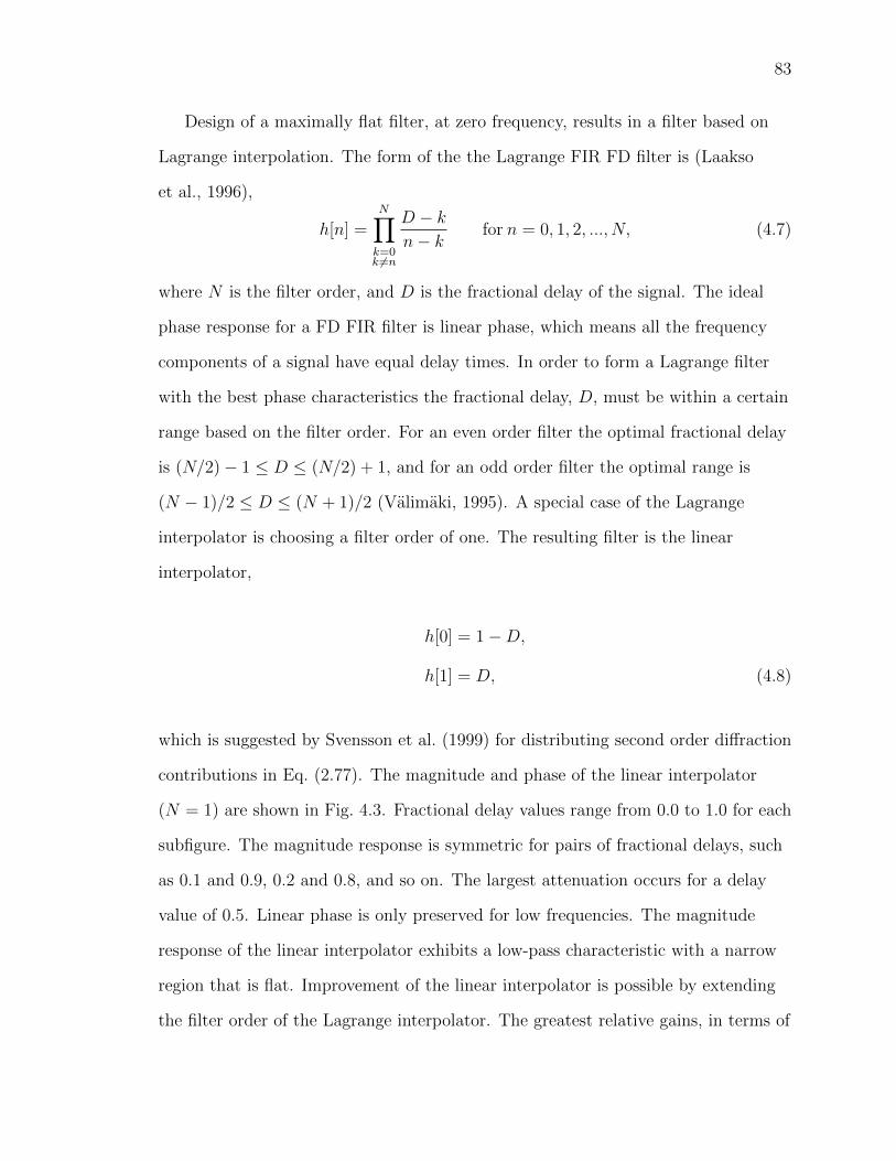
83
Design of a maximally flat filter, at zero frequency, results in a filter based on
Lagrange interpolation. The form of the the Lagrange FIR FD filter is (Laakso
et al., 1996),
h[n] =N∏k=0k 6=n
D − kn− k
for n = 0, 1, 2, ..., N, (4.7)
where N is the filter order, and D is the fractional delay of the signal. The ideal
phase response for a FD FIR filter is linear phase, which means all the frequency
components of a signal have equal delay times. In order to form a Lagrange filter
with the best phase characteristics the fractional delay, D, must be within a certain
range based on the filter order. For an even order filter the optimal fractional delay
is (N/2)− 1 ≤ D ≤ (N/2) + 1, and for an odd order filter the optimal range is
(N − 1)/2 ≤ D ≤ (N + 1)/2 (Valimaki, 1995). A special case of the Lagrange
interpolator is choosing a filter order of one. The resulting filter is the linear
interpolator,
h[0] = 1−D,
h[1] = D, (4.8)
which is suggested by Svensson et al. (1999) for distributing second order diffraction
contributions in Eq. (2.77). The magnitude and phase of the linear interpolator
(N = 1) are shown in Fig. 4.3. Fractional delay values range from 0.0 to 1.0 for each
subfigure. The magnitude response is symmetric for pairs of fractional delays, such
as 0.1 and 0.9, 0.2 and 0.8, and so on. The largest attenuation occurs for a delay
value of 0.5. Linear phase is only preserved for low frequencies. The magnitude
response of the linear interpolator exhibits a low-pass characteristic with a narrow
region that is flat. Improvement of the linear interpolator is possible by extending
the filter order of the Lagrange interpolator. The greatest relative gains, in terms of

84
0 0.2 0.4 0.6 0.8 1
0
0.2
0.4
0.6
0.8
10.0
0.1
0.2
0.3
0.4
0.5
Normalized Frequency
Mag
nit
ude
(a)
0 0.2 0.4 0.6 0.8 1
0
0.2
0.4
0.6
0.8
1
0.0
0.1
0.2
0.3
0.4
0.5
0.6
0.7
0.8
0.9
1.0
Normalized Frequency
Phas
eD
elay
[sam
ple
s]
(b)
Figure 4.3: First order (N = 1) Lagrange fractional delay finite impulse responsefilter (linear interpolator). (a) Magnitude responses for eleven fractional delays, from0.0 to 1.0. The magnitude responses are symmetric such that a fractional delay of0.9 overlaps a fractional delay of 0.1. (b) Phase delay responses for eleven fractionaldelays, from 0.0 to 1.0.
widening the low-pass band and preserving linear phase, results from increasing the
filter order to three. Figure 4.4 shows the magnitude and phase of the third order
(N = 3) Lagrange interpolator. Compared to the linear interpolator the third order
Lagrange interpolator has a wider low-pass band. For example, given a fractional
delay of 1.5, a 0.1 dB or larger attenuation occurs for frequencies greater than 27%
of the Nyquist frequency. The same attenuation for a linear interpolator, and a
fractional delay of 0.5, occurs for frequencies greater than 10% of the Nyquist
frequency.
Based on the advantages of a short filter length, good low-pass bandwidth, and
linear phase characteristics the third-order Lagrange interpolator is utilized for the
digital synthesis of direct, reflected, second-order diffraction, and higher-order
diffraction impulse responses in the present study. Broadband frequency responses,
with little magnitude and phase distortion, are possible by setting the sampling

85
0 0.2 0.4 0.6 0.8 1
0
0.2
0.4
0.6
0.8
11.0
1.1
1.2
1.3
1.4
1.5
Normalized Frequency
Mag
nit
ude
(a)
0 0.2 0.4 0.6 0.8 1
1
1.2
1.4
1.6
1.8
2
1.0
1.1
1.2
1.3
1.4
1.5
1.6
1.7
1.8
1.9
2.0
Normalized Frequency
Phas
eD
elay
[sam
ple
s]
(b)
Figure 4.4: Third order Lagrange fractional delay finite impulse response filter. (a)Magnitude responses for eleven fractional delays, from 1.0 to 2.0. The magnituderesponses are symmetric such that a fractional delay of 1.9 overlaps a fractional delayof 1.1. (b) Phase delay responses for eleven fractional delays, from 1.0 to 2.0.
frequency to 160 kHz. Frequency responses in the range of 0 to 20 kHz have
negligible magnitude and phase distortion. Digital synthesis of first-order diffraction
is treated separately by increasing the sampling frequency to 800 kHz and
resampling the resulting impulse response down to 160 kHz. The resampling is
necessary in order to combine first-order diffraction impulse responses with other
impulse responses.
4.4 Verification Cases
The fusion of adaptive tetrahedral tracing and a secondary source model for edge
diffraction is numerically validated against three test cases. The adaptive
tetrahedral tracing algorithm, and interface with the edge diffraction model were
coded in MATLAB. The edge diffraction model was coded by Peter Svensson, in
MATLAB. The first test case is on the scattering of a rigid acoustic wedge. The

86
second test case is on the scattering of a rigid panel. The third test case is on the
scattering of a triangular diffusor. For the first test case numerical results are
compared against an asymptotic formulation of diffraction. For the last two test
cases numerical results are compared against BEM predictions. The first test case
illustrates the capability of the adaptive tetrahedral tracing procedure to identify
wedge parameters for first order diffraction calculations. The second test case
demonstrates a capability for calculating higher-order diffraction and geometric
reflection. Lastly, the third test case demonstrates the limitations on computing a
finite number of reflection and diffraction permutations.
4.4.1 Rigid Acoustic Wedge
The acoustic scattering of a rigid acoustic wedge, with a closed wedge angle, θWC , of
π/2 is computed with adaptive tetrahedral tracing and a secondary source model for
edge diffraction, and compared with an asymptotic formulation for diffraction
(Pierce, 1974; Hadden, Jr. and Pierce, 1981). The source and receiver have
cylindrical coordinates (rS = 1, θS = 4π/3, zS = 0) and (rR = 3, θR = π/4, zR = 0),
respectively. The diffraction formulation by Pierce (1974) is based on acoustic
diffraction from an infinitely long wedge. The geometry of the tested scenario is
shown in Fig. 4.5.
A portion of the total acoustic field is composed of free field radiation and
geometric propagation, referred hereafter as the geometric acoustic sound field. In
(Pierce, 1974) a time dependence of e−iωt is assumed; however, a time dependence of
ejωt is used for the following variable definitions. Geometric parameters
corresponding to source, receiver, and wedge face angles are the basis for the

87
θ = 0
θ=θ W
θWC
θS
θR
rS
rR
S
R
Figure 4.5: Right angled wedge geometry for comparing hybrid method and Pierce’sformulation for wedge diffraction. The closed wedge angle, θWC , is π/2. The source,S, has the following cylindrical coordinates: (rS = 1, θS = 4π/3, zS = 0). Thereceiver, R, has the following cylindrical coordinates: (rR = 3, θR = π/4, zR = 0).
geometric acoustic sound field (Hadden, Jr. and Pierce, 1981),
θ1 = |θS − θR|, (4.9a)
θ2 = θS + θR, (4.9b)
θ3 = 2θW − (θS + θR), (4.9c)
θ4 = 2θW − |θS − θR|, (4.9d)
where θ1 is the exterior angle formed by the source and receiver, θ2 is the exterior
angle formed by the source reflected about the θ = 0 plane and receiver, θ3 is the
exterior angle formed by the source reflected about the θ = θW plane and receiver,
and θ4 is the exterior angle formed by the source reflected about the θ = θW plane
and the receiver reflected about the θ = 0 plane. Each of the above parameters
corresponds to a component of the geometric sound field. The angle θ1 corresponds
to the direct wave, θ2 corresponds to the wave reflected from the θ = 0 plane, θ3
corresponds to the wave reflected from the θ = θW plane, and θ4 corresponds to the

88
wave reflected from the θ = 0 and θ = θW planes. The total geometric sound field,
cast as a Green’s function, is given as a sum of each geometric component,
G(~rS;~rR)G =4∑i=1
e−jkRi
Ri
H(π − θi), (4.10)
where GG is the geometric acoustic Green’s function from the source position ~rS to
the receiver position ~rR, H(π − θi) is the Heaviside step function, e−jkRi/Ri
represents a spherically diverging wave, and Ri represents the distance from the
(image) source to the (image) receiver,
Ri =√r2S + r2
R + (zS − zR)2 − 2rRrS cos θi. (4.11)
To complete the computation of the sound field the diffracted sound field must be
considered.
The diffracted sound field is formulated through an asymptotic expansion of a
contour integral. The Green’s function for diffraction is (Pierce, 1974),
G(~rS;~rR)D =e−jkL0
L0
e−jπ/4√2
(S+ + S−), (4.12)
where L0 is the least time path from the source to the receiver; see Sec. 2.6.1. The
variable S± = S(θR ± θS) is similar to all other variables with a plus or minus
subscript, and is defined as,
S± =π(1 + ∆±)W±AD(W±)−∆±
πX±, (4.13)
where X± = X(θR ± θS), W± = W (θR ± θS), and ∆± = ∆(θR ± θS). Each of the

89
variables in S± are defined as,
X(θ) = γMν(θ), (4.14a)
W (θ) = γNν(θ), (4.14b)
∆(θ) =cos(νπ)
2
cos(νπ)− cos(νθ)
1− cos(νπ) cos(νθ), (4.14c)
where ν = π/θW is the wedge index and,
Mν(θ) =cos(νπ)− cos(νθ)
ν sin(νπ), (4.15a)
Nν(θ) =cos(νπ)− cos(νθ)
ν√
1− cos(νπ) cos(νθ), (4.15b)
γ =
√2rSrRλL0
, (4.15c)
where λ = c/f is the acoustic wavelength. The parameter AD(W ) is defined as,
AD(W ) = sign(W )[f(|W |) + jg(|W |)], (4.16)
where the auxiliary Fresnel functions f(W ) and g(W ) are defined in terms of the
Fresnel integrals,
f(W ) = [(1/2)− S(W )] cos([1/2]πW 2)
− [(1/2)− C(W )] sin([1/2]πW 2), (4.17a)
g(W ) = [(1/2)− C(W )] cos([1/2]πW 2)
+ [(1/2)− S(W )] sin([1/2]πW 2), (4.17b)

90
and the Fresnel cosine and sine integrals are,
C(W ) =
∫ |W (θ)|
0
cos([1/2]πt2) dt, (4.18a)
S(W ) =
∫ |W (θ)|
0
sin([1/2]πt2) dt. (4.18b)
The Fresnel integrals are computed by adaptive Simpson quadrature (Gander and
Gautschi, 2000). The total sound field is simply a summation of geometric and
diffraction Green’s functions from Eqs. (4.10) and (4.12).
A reasonable comparison between the hybrid method and Pierce’s method,
which assumes an infinite wedge, requires a sufficiently long finite wedge. The reason
is the low frequency response is dictated by the decaying tail of diffraction, which is
affected by the length of the wedge. A longer wedge results in a longer diffraction
tail. A wedge 40 m long was computed with the adaptive tetrahedral tracing edge
diffraction method. The length is sufficiently long such that the frequency response
at low frequencies does not change considerably given a longer wedge.
In order to compare the results against Pierce’s formulation a transfer function
is generated for each respective solution. The transfer function is computed relative
to free field radiation at 1 m. The conversion of the transient impulse response,
Eq. (4.3), to the frequency domain is conducted by a Fast Fourier Transform,
through a MATLAB subroutine. The transfer function relative to free field
radiation at 1 m is computed as,
TF = 20 log10(|H|), (4.19)
where H is either the complex frequency response of the impulse response, or the
summation of Green’s functions from Eqs. (4.10) and (4.12).
Figure 4.6 compares the adaptive tetrahedral tracing and edge diffraction results
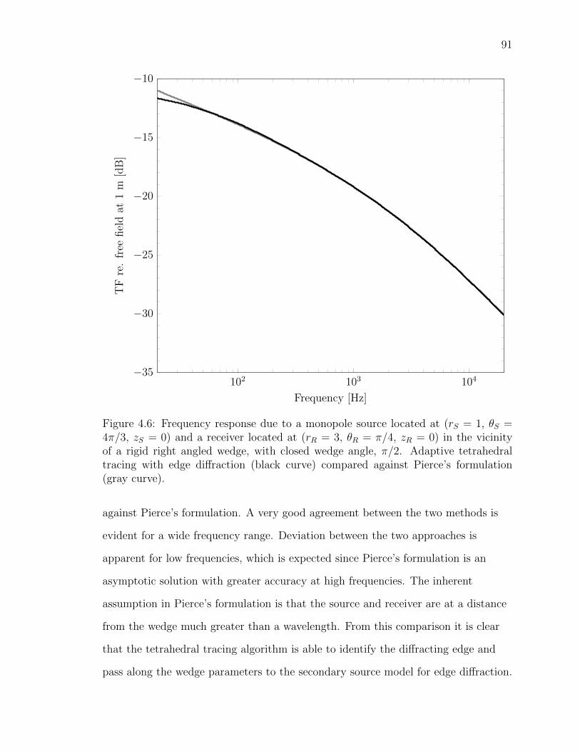
91
102 103 104
−10
−15
−20
−25
−30
−35
Frequency [Hz]
TF
re.
free
fiel
dat
1m
[dB
]
Figure 4.6: Frequency response due to a monopole source located at (rS = 1, θS =4π/3, zS = 0) and a receiver located at (rR = 3, θR = π/4, zR = 0) in the vicinityof a rigid right angled wedge, with closed wedge angle, π/2. Adaptive tetrahedraltracing with edge diffraction (black curve) compared against Pierce’s formulation(gray curve).
against Pierce’s formulation. A very good agreement between the two methods is
evident for a wide frequency range. Deviation between the two approaches is
apparent for low frequencies, which is expected since Pierce’s formulation is an
asymptotic solution with greater accuracy at high frequencies. The inherent
assumption in Pierce’s formulation is that the source and receiver are at a distance
from the wedge much greater than a wavelength. From this comparison it is clear
that the tetrahedral tracing algorithm is able to identify the diffracting edge and
pass along the wedge parameters to the secondary source model for edge diffraction.

92
4.4.2 Rigid Panel
Acoustic scattering of a rigid panel, 3.6 m wide, is compared between the adaptive
tetrahedral tracing edge diffraction method and BEM results (Cox and D’Antonio,
2011). An array of 37 receivers surround the panel, separated at five degree
intervals, 50 m away from the center of the panel. A source is normal to the panel
center and 100 m away. The source and receiver configuration correspond to BEM
calculations (Cox and D’Antonio, 2009, p. 134). The length of the scattering panel
is set to 20 m long in order to compare three-dimensional results (adaptive
tetrahedral tracing and edge diffraction) against two-dimensional results (BEM).
The BEM calculations are based on the thin-panel assumption applied to the
Kirchhoff-Helmholtz equation; see Eq. (2.23). The thin-panel assumption casts the
problem in terms of pressure differences and pressure sums across the thin panel.
The derivative of Eq. (2.23) is used with the original equation in order to
simultaneously solve for pressures at the front and back of a surface (Terai, 1980).
The thin-panel BEM is based on Eqs. (2.29)–(2.31).
A comparison of the adaptive tetrahedral tracing edge diffraction method with
the BEM is made across one-third octave bands. One-third octave band spectra are
computed by a conversion of frequency points corresponding to 1/18-octave band
center frequencies to 1/3-octave band spectra. The 1/18-octave band center
frequencies are computed according to a base ten system (S1, 1986),
fm = fr(Uk), (4.20)
where fm is the center frequency of each 1/18-octave band, fr is the reference
frequency (1000 Hz), k is an integer value, and the frequency ratio U is,
U = 10(3b/10), (4.21)
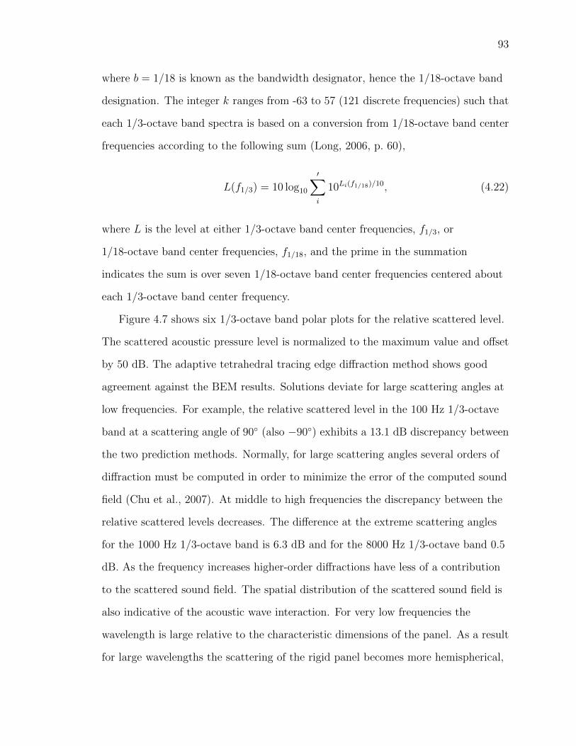
93
where b = 1/18 is known as the bandwidth designator, hence the 1/18-octave band
designation. The integer k ranges from -63 to 57 (121 discrete frequencies) such that
each 1/3-octave band spectra is based on a conversion from 1/18-octave band center
frequencies according to the following sum (Long, 2006, p. 60),
L(f1/3) = 10 log10
′∑i
10Li(f1/18)/10, (4.22)
where L is the level at either 1/3-octave band center frequencies, f1/3, or
1/18-octave band center frequencies, f1/18, and the prime in the summation
indicates the sum is over seven 1/18-octave band center frequencies centered about
each 1/3-octave band center frequency.
Figure 4.7 shows six 1/3-octave band polar plots for the relative scattered level.
The scattered acoustic pressure level is normalized to the maximum value and offset
by 50 dB. The adaptive tetrahedral tracing edge diffraction method shows good
agreement against the BEM results. Solutions deviate for large scattering angles at
low frequencies. For example, the relative scattered level in the 100 Hz 1/3-octave
band at a scattering angle of 90 (also −90) exhibits a 13.1 dB discrepancy between
the two prediction methods. Normally, for large scattering angles several orders of
diffraction must be computed in order to minimize the error of the computed sound
field (Chu et al., 2007). At middle to high frequencies the discrepancy between the
relative scattered levels decreases. The difference at the extreme scattering angles
for the 1000 Hz 1/3-octave band is 6.3 dB and for the 8000 Hz 1/3-octave band 0.5
dB. As the frequency increases higher-order diffractions have less of a contribution
to the scattered sound field. The spatial distribution of the scattered sound field is
also indicative of the acoustic wave interaction. For very low frequencies the
wavelength is large relative to the characteristic dimensions of the panel. As a result
for large wavelengths the scattering of the rigid panel becomes more hemispherical,

94
resembling point scattering. For higher frequencies a single strong lobe is generated
indicative of the strong specular reflection in the normal direction. The lobe
broadens as the frequency decreases due to the increasing influence of diffraction.
The root-mean-square error (RMSE) is computed between the adaptive
tetrahedral tracing edge diffraction method and the BEM. The RMSE is computed
as,
RMSE(f1/3) =
√√√√ N∑i=1
[LATTED(f1/3)− LBEM(f1/3)
]2/N, (4.23)
where N = 37 is the total number of receivers, LATTED is the 1/3-octave band
spectra for the adaptive tetrahedral tracing edge diffraction method, and LBEM is
the 1/3-octave band spectra for the BEM. One-third-octave bands ranging from 100
Hz to 8000 Hz, with various orders of diffraction included in the calculation are
shown in Table 4.1. Generally, the RMSE increases as the frequency decreases. The
result is expected since the inclusion of a finite number of diffraction orders results
in an approximation of the acoustic field. The inclusion of higher orders of
diffraction results in lower RMSE values, which is expected since the approximate
solution converges to the actual sound field by including higher orders of diffraction.
However, little to no reduction in the RMSE is evident by the inclusion of
third-order diffraction. Compared to the peak magnitude of second-order
diffraction, third-order diffraction is two orders of magnitude smaller. However, a
systematic error may be present due to neglecting slope diffraction. Depending
upon the accuracy required, and the problem geometry, calculations including first-
or second-order diffraction may suffice.
4.4.3 Triangular Diffusor
Acoustic scattering of a geometric diffusor is compared between the adaptive
tetrahedral tracing edge diffraction method and the BEM (Cox and D’Antonio,
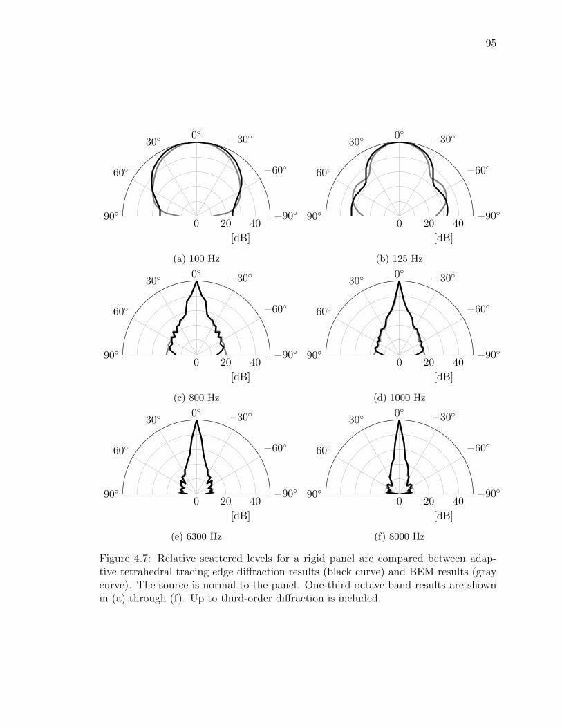
95
−90
−60
−30030
60
900 20 40
[dB]
(a) 100 Hz
−90
−60
−30030
60
900 20 40
[dB]
(b) 125 Hz
−90
−60
−30030
60
900 20 40
[dB]
(c) 800 Hz
−90
−60
−30030
60
900 20 40
[dB]
(d) 1000 Hz
−90
−60
−30030
60
900 20 40
[dB]
(e) 6300 Hz
−90
−60
−30030
60
900 20 40
[dB]
(f) 8000 Hz
Figure 4.7: Relative scattered levels for a rigid panel are compared between adap-tive tetrahedral tracing edge diffraction results (black curve) and BEM results (graycurve). The source is normal to the panel. One-third octave band results are shownin (a) through (f). Up to third-order diffraction is included.

96
Table 4.1: Root-mean-square error (RMSE) of the relative scattered pressure levelsfor rigid panel scattering between the adaptive tetrahedral tracing edge diffractionmodel and the BEM. Source is normal to finite panel.
RMSE [dB]
1/3 Octave Diffraction Order IncludedBand [Hz] First Second Third
100 5.9 3.4 3.5125 4.4 3.2 3.1160 3.7 2.4 2.4200 2.4 2.3 2.4250 1.5 1.0 1.0315 1.2 1.7 1.7400 1.6 2.4 2.4500 1.5 2.2 2.2630 1.9 2.7 2.7800 1.2 2.1 2.01000 0.8 1.7 1.71250 1.1 0.9 0.91600 2.4 1.5 1.62000 1.0 0.9 0.92500 1.2 1.6 1.63150 1.6 1.0 1.04000 0.6 1.0 1.05000 0.6 1.5 1.46300 0.8 0.9 0.98000 1.1 0.6 0.6
97
2011). The geometric diffusor is a triangular diffusor that is 3.66 m wide with three
periods of triangles. Each triangular profile forms an isosceles triangle with two
congruent angles of 18 at the base of each triangle. The choice of a triangular
diffusor is motivated by the fact that multiple specular reflections occur and the the
effect of omitting certain permutations of diffraction is illustrated.
Figure 4.8 shows six 1/3-octave band relative scattered levels for the triangular
diffusor. In this particular case the source is oblique to the normal by 57. The
overall character of the acoustic scattering is captured at low frequencies; however,
large discrepancies are evident. The reason for the discrepancy must be due to the
omission of certain diffraction permutations. Second-order diffraction that is the
result of one edge scattering event, a reflection, and another edge scattering event
may be particularly important for this geometry. As the frequency increases the
agreement improves for the adaptive tetrahedral tracing edge diffraction method. It
is interesting to note that the main scattering lobe at low frequencies corresponds to
the specular reflection angle; however, a stronger lobe away from the specular angle
exists at higher frequencies. The strong scattering in the direction of −20 and
−90 is due to the geometry of the triangular profiles. For a normally incident
sound field the primary lobes occur at 36 and −36, which is twice the acute angle
of each triangle (Cox and D’Antonio, 2009, p. 340). For an oblique incident sound
field it is expected that the lobes have the same relative position with respect to the
scattering angle, which is confirmed in Figs. 4.8(e) and 4.8(f). Based on a
separation of 36 from the specular angle it is expected the main lobes to appear at
−21 and −93. According to Figs. 4.8(e) and 4.8(f) it can be seen that the main
lobes correspond to what is expected geometrically.
The root-mean-square error (RMSE) is computed between the adaptive
tetrahedral tracing edge diffraction method and the BEM. One-third octave bands
ranging from 100 Hz to 8000 Hz, with various orders of diffraction included in the

98
−90
−60
−30030
60
900 20 40
[dB]
(a) 100 Hz
−90
−60
−30030
60
900 20 40
[dB]
(b) 125 Hz
−90
−60
−30030
60
900 20 40
[dB]
(c) 800 Hz
−90
−60
−30030
60
900 20 40
[dB]
(d) 1000 Hz
−90
−60
−30030
60
900 20 40
[dB]
(e) 6300 Hz
−90
−60
−30030
60
900 20 40
[dB]
(f) 8000 Hz
Figure 4.8: Relative scattered levels for a rigid triangular diffusor are compared be-tween adaptive tetrahedral tracing edge diffraction results (black curve) and BEMresults (gray curve). The source is oblique to the normal at 57. One-third octaveband results are shown in (a) through (f). Up to second-order diffraction is included.

99
calculation are shown in Table 4.2. Generally, the RMSE increases as the frequency
decreases. The result is expected since the inclusion of a finite number of diffraction
orders results in an approximation of the acoustic field. Compared to the rigid
panel, Table 4.1, the RMSE at high frequencies is consistently 2 dB above. The
inclusion of higher orders of diffraction generally results in lower RMSE values;
however, for very low frequencies inclusion of third-order diffraction increases the
RMSE. This artifact must be due to physically incorrect diffraction paths computed
according to the enumeration procedure in Sec. 4.2. For mid- to high-frequency
computations the adaptive beam tracing edge diffraction method is well-suited for
diffusor scattering prediction.
Table 4.2: Root-mean-square error (RMSE) of the relative scattered pressure levelsfor rigid triangular diffusor scattering between the adaptive tetrahedral tracing edgediffraction model and the BEM. Source is oblique with an angle of incidence 57.
RMSE [dB]
1/3 Octave Diffraction Order IncludedBand [Hz] First Second Third
100 9.8 7.3 8.9125 9.3 6.1 8.2160 10.0 5.5 6.8200 10.3 5.4 5.7250 8.1 4.8 4.3315 7.1 3.6 3.3400 6.5 4.4 4.1500 7.0 4.3 4.6630 6.1 4.1 4.5800 4.8 4.3 4.81000 4.7 4.5 4.41250 5.0 5.2 4.91600 3.8 3.8 3.82000 3.6 3.4 3.12500 3.7 3.3 3.23150 3.6 3.3 3.34000 3.4 3.3 3.25000 3.2 3.0 3.06300 3.3 3.3 3.38000 3.0 3.0 3.0

100
4.5 Summary
The compatibility of the adaptive tetrahedral tracing algorithm is based upon a link
that exists between the acoustic mapping and the identification of edge diffraction.
It was shown how wedge parameters are extracted from the acoustic mapping and
passed along to the secondary source model for edge diffraction. Higher-order
diffraction requires a procedure to enumerate the multitude of diffraction paths.
Utilizing the concept of a directed graph and modified graph searching algorithms
the multitude of higher-order diffraction paths are identified. The process of
adaptive tetrahedral tracing results in determining the geometric acoustic field. The
diffracted sound field is computed by the secondary source model for edge
diffraction. The digital synthesis of an impulse response is considered as a linear
combination of the free-field radiation, geometric acoustics, and diffracted sound.
Fractional delays corresponding to exact arrival times are handled by a third-order
Lagrange interpolator. Finally, numerical verification of the combined adaptive
tetrahedral tracing algorithm and secondary source model for edge diffraction is
based upon three test cases. The scattering characteristics of a rigid right-angled
wedge, rigid panel, and rigid triangular diffusor are compared against analytic and
BEM results. It is shown that the adaptive tetrahedral tracing edge diffraction
method is particularly well-suited to compute the scattering characteristics of a
panel and triangular diffusor at mid- to high-frequencies.
Chapter 5
Goniometer Measurements
The measurement of the scattered impulse response for a diffusor is accomplished
with an instrument known as a goniometer. The principle of the diffusor
measurement is based on estimating the scattered impulse response by deconvolving
the loudspeaker-microphone transfer function from the subtracted impulse response.
The subtracted impulse response is a subtraction of the impulse response with the
diffusor present, and without the diffusor present. The subtraction is conducted in
order to eliminate the direct sound.
In the present study a boundary layer goniometer is employed for the
measurement of acoustic diffusors. The instrument is a fixed semicircular
microphone array with a diffusor at the center of the array and a loudspeaker
outside of the array emitting an interrogating signal; see Fig. 5.2. Two types of
stimuli are tested: a maximum length sequence (MLS) and a logarithmic swept-sine
(LSS). The merits of either signal are compared and contrasted.
Section 5.1 introduces the theoretical concepts that form the basis of a
goniometer measurement. The signal processing involved in the measurement
procedure are shown to produce an estimate of the scattered impulse response of an
acoustic diffusor. In Sec. 5.2 the specific instrumentation of the goniometer is
101
102
described. The arrangement of the measurement apparatus is shown in detail. A
comparison between measured polar responses and predicted polar responses, by the
adaptive tetrahedral tracing edge diffraction method, are given in Sec. 5.3. Lastly, a
summary is given in Sec. 5.4.
5.1 Theoretical Aspects of a Goniometer
Measurement
A goniometer is a multi-microphone array that measures the scattered signal of a
diffusor excited by a single loudspeaker. In order to arrive at the scattered polar
response, the scattered impulse response must be estimated from the measurement.
Three essential measurements are necessary for estimating the scattered impulse
response (Cox and D’Antonio, 2009, pp. 111-121). The first measurement is the
loudspeaker-to-microphone measurement. The purpose of the
loudspeaker-to-microphone measurement is to characterize the transfer path
between the loudspeaker and each microphone. This measurement captures the
magnitude and phase distortion introduced by the measurement equipment. The
second measurement, called the sample measurement, is conducted with the diffusor
placed at the center of the microphone array. In this measurement the direct and
scattered signals are measured by the array. The third measurement, called the
background measurement, is conducted with no diffusor present. This last
measurement captures the direct signal measured by the array. Each of these
measurements is fundamental to estimating the scattered impulse response.
5.1.1 Estimation of the Scattered Impulse Response
It is important to stress that the scattered impulse response is an estimated impulse
response. Analysis of the measured signals in the discrete-time domain show how
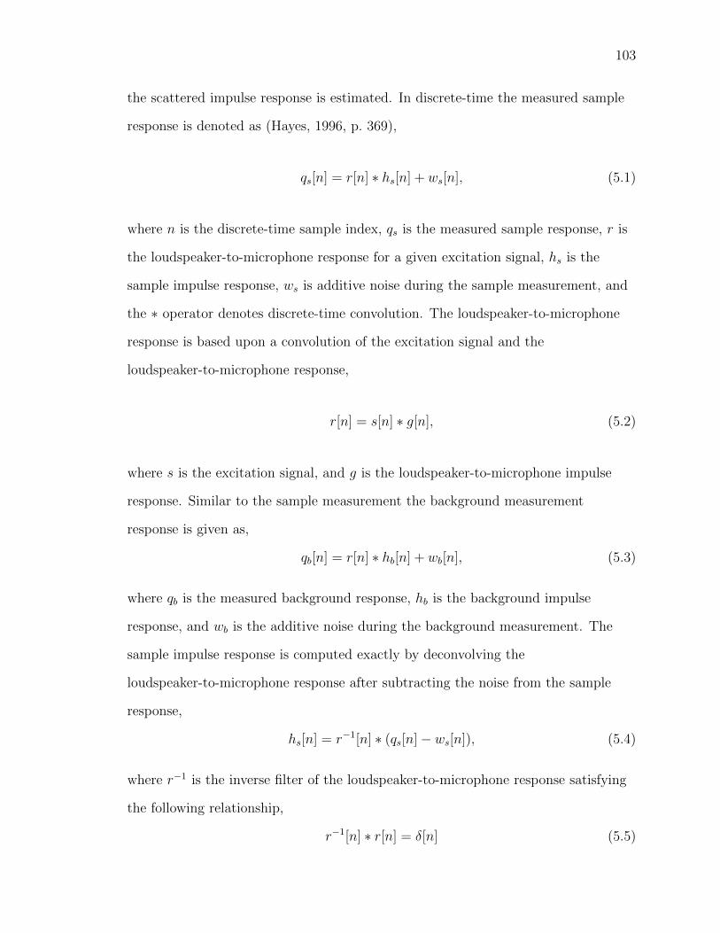
103
the scattered impulse response is estimated. In discrete-time the measured sample
response is denoted as (Hayes, 1996, p. 369),
qs[n] = r[n] ∗ hs[n] + ws[n], (5.1)
where n is the discrete-time sample index, qs is the measured sample response, r is
the loudspeaker-to-microphone response for a given excitation signal, hs is the
sample impulse response, ws is additive noise during the sample measurement, and
the ∗ operator denotes discrete-time convolution. The loudspeaker-to-microphone
response is based upon a convolution of the excitation signal and the
loudspeaker-to-microphone response,
r[n] = s[n] ∗ g[n], (5.2)
where s is the excitation signal, and g is the loudspeaker-to-microphone impulse
response. Similar to the sample measurement the background measurement
response is given as,
qb[n] = r[n] ∗ hb[n] + wb[n], (5.3)
where qb is the measured background response, hb is the background impulse
response, and wb is the additive noise during the background measurement. The
sample impulse response is computed exactly by deconvolving the
loudspeaker-to-microphone response after subtracting the noise from the sample
response,
hs[n] = r−1[n] ∗ (qs[n]− ws[n]), (5.4)
where r−1 is the inverse filter of the loudspeaker-to-microphone response satisfying
the following relationship,
r−1[n] ∗ r[n] = δ[n] (5.5)

104
where δ is the Kronecker delta function. Similarly the background impulse response
is computed exactly by a deconvolution,
hb[n] = r−1[n] ∗ (qb[n]− wb[n]). (5.6)
The scattered impulse response is determined exactly by subtracting the sample
impulse response, Eq. (5.4), from the background impulse response, Eq. (5.6),
hsc[n] = hs[n]− hb[n] = r−1[n] ∗ (qs[n]− qb[n]) + r−1[n] ∗ (wb[n]− ws[n]), (5.7)
where hsc is the scattered impulse response.
In practice it is assumed the additive noise in the sample and background
measurements is negligible (AES Standards Committee, 2001). If the signal-to-noise
ratio is high enough, then neglecting noise is a reasonable assumption. The
subtraction process does not completely eliminate the direct and reflected sound due
to time-variance. Instead, the process decreases the contributions of direct and
reflected sound within the scattered impulse response. A rectangular weighting is
then applied to the time region when sound scattering occurs in order to eliminate
to a large extent the direct and reflected sound residuals in the subtracted impulse
response. Hence, the scattered impulse response is estimated as,
hsc[n] = w[n](hs[n]− hb[n]) = w[n](r−1[n] ∗ (qs[n]− qb[n])
), (5.8)
where w[n] is a rectangular weighting applied to time samples when acoustic
scattering is present, and the hat above each impulse response indicates an estimate
of the impulse response. Furthermore, the processing of each measured signal is
generally conducted in the frequency domain. For example, the estimated scattered
impulse response is computed in the discrete frequency domain by a N -point

105
discrete Fourier transform (DFT) of the respective signals,
Hsc[k] =Qs[k]−Qb[k]
R[k]=Qs[k]−Qb[k]
S[k]G[k]for k = 0,...,N - 1, (5.9)
where the index k corresponds to discrete frequencies. Caution must be exercised
when conducting a deconvolution in the time-domain. Due to the inherent
periodicity of the DFT, the number of points of the DFT, N , must be at least equal
to the signal length of the subtracted measurements plus the signal length of the
loudspeaker-microphone response. The scattered impulse response is then computed
by an inverse DFT of the result in Eq. (5.9). It is preferred to process the signals in
the frequency domain since the division operation effectively deconvolves the
signal(s) in the denominator, which is a faster operation by the Fast Fourier
Transform (FFT) than by deconvolution in the discrete-time domain (Oppenheim
et al., 1999, p. 655).
An important consideration in measuring the scattered signal is the necessary
condition for recovering the scattered impulse response. The arrangement of a
loudspeaker, microphone array, and an acoustic diffusor within a testing space must
be such that no reflections contaminate the time window for acoustic scattering, and
the direct to scattered signals are separated well enough in time. A quasi-anechoic
setup was developed by D’Antonio and Konnert (1992) to satisfy this necessary
condition. Later, the arrangement of the loudspeaker and microphone array was
optimized to maintain a specific specular region width, and a quasi-anechoic
condition (D’Antonio and Rife, 2011). Further details on the quasi-anechoic
conditions are in Sec. 5.2.2.

106
5.1.2 Excitation Signal
The choice of excitation signal is particularly important for the estimation of the
scattered impulse response. The ideal signal is broadband in nature, exhibits a high
signal-to-noise ratio, and is short in length. Of the available excitation signals three
general categories exist: periodic signals, transient, and non-transient aperiodic
(Schoukens et al., 1988). Periodic signal types include stepped sinusoid, swept sine,
multisine, periodic noise, maximum length binary sequence, and discrete interval
binary sequence. Transient signal types include impulse and random burst. Lastly,
an aperiodic signal is random noise. A comparison of all the signals mentioned
above shows that deterministic signals such as the swept-sine, multisine, and
maximum length binary sequence are very good at estimating the transfer function
in the presence of a flat noise spectrum (Schoukens et al., 1988).
Early measurements of acoustic diffusors utilized a system employing time-delay
spectrometry (TDS) (D’Antonio and Konnert, 1992). A single microphone was used
for the measurement of a semicircular polar response. The excitation signal in a
TDS measurement is a linearly swept-sinusoidal signal (Muller and Massarani,
2001). The principle behind the measurement technique is based on the modulation
theorem (Oppenheim et al., 1999, pp. 61, 62). A delayed excitation signal is
modulated with the received signal producing sum and difference products of the
signal. If the delay corresponds to the acoustic path of the excitation signal from
the loudspeaker, then the difference product is ideally at the DC frequency.
Low-pass filtering removes the sum product from the frequency response, effectively
isolating the frequency response of the acoustic diffusor. Some drawbacks of the
technique include long measurement times and the delicate setting for the
modulated signal delay (Poletti, 1988). After some time TDS was replaced in favor
of an alternative excitation signal.
The maximum length sequence (MLS) is currently the excitation signal of choice

107
for acoustic diffusor measurement (D’Antonio, 1995, pp. 112, 113). The excitation
signal is based on a binary sequence generated by a feedback shift register
(MacWilliams and Sloane, 1976; Vanderkooy, 1994). A MLS is categorized as a
psuedorandom periodic sequence. The signal length is dependent on the order of the
feedback shift register,
L = 2m − 1, (5.10)
where m is the order number, and L is the periodic length of the sequence. The
circular autocorrelation of an MLS signal is nearly a Kronecker delta function and
the energy density spectrum of the circular autocorrelation is white, except at DC
(Vanderkooy, 1994). The advantage of using an MLS signal is the broadband nature
of the signal, and no need for averaging. Furthermore, when compared to TDS the
use of an MLS signal allows quicker measurement times and better frequency
resolution (Vanderkooy, 1994). If the noise spectrum in the measurement is not flat,
then the MLS may be preemphasized in the frequency domain in order to achieve a
uniform signal-to-noise ratio (Mommertz and Muller, 1995). Disadvantages
associated with the use of a MLS signal include the nonuniform distribution of
harmonic distortion in the recovered impulse response, the required fine tuning of
the gain to minimize harmonic distortion and maximize the signal-to-noise ratio,
sensitivity to time-variance, and the enhancement of harmonic distortion by
averaging (Muller and Massarani, 2001; Vanderkooy, 1994). Since the harmonic
distortion is non-uniformly distributed throughout the causal part of the impulse
response, it contaminates the estimated impulse response without remedy
(Vanderkooy, 1994).
Another measurement signal well-suited for acoustic diffusor measurement is the
logarithmic swept-sine (LSS). Similar to the linear swept-sine the logarithmic
swept-sine is a frequency modulated sinusoidal signal with advantageous properties.
The advantages of a LSS signal include a higher signal-to-noise ratio compared to
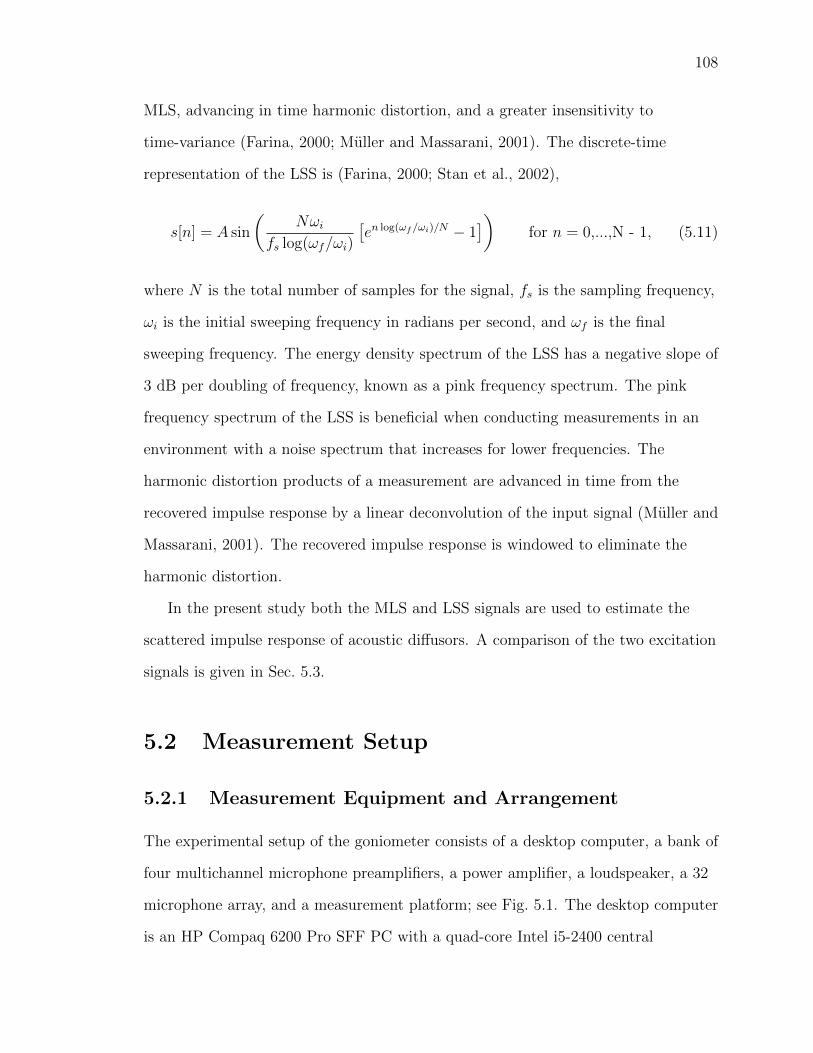
108
MLS, advancing in time harmonic distortion, and a greater insensitivity to
time-variance (Farina, 2000; Muller and Massarani, 2001). The discrete-time
representation of the LSS is (Farina, 2000; Stan et al., 2002),
s[n] = A sin
(Nωi
fs log(ωf/ωi)
[en log(ωf/ωi)/N − 1
])for n = 0,...,N - 1, (5.11)
where N is the total number of samples for the signal, fs is the sampling frequency,
ωi is the initial sweeping frequency in radians per second, and ωf is the final
sweeping frequency. The energy density spectrum of the LSS has a negative slope of
3 dB per doubling of frequency, known as a pink frequency spectrum. The pink
frequency spectrum of the LSS is beneficial when conducting measurements in an
environment with a noise spectrum that increases for lower frequencies. The
harmonic distortion products of a measurement are advanced in time from the
recovered impulse response by a linear deconvolution of the input signal (Muller and
Massarani, 2001). The recovered impulse response is windowed to eliminate the
harmonic distortion.
In the present study both the MLS and LSS signals are used to estimate the
scattered impulse response of acoustic diffusors. A comparison of the two excitation
signals is given in Sec. 5.3.
5.2 Measurement Setup
5.2.1 Measurement Equipment and Arrangement
The experimental setup of the goniometer consists of a desktop computer, a bank of
four multichannel microphone preamplifiers, a power amplifier, a loudspeaker, a 32
microphone array, and a measurement platform; see Fig. 5.1. The desktop computer
is an HP Compaq 6200 Pro SFF PC with a quad-core Intel i5-2400 central

109
D
S
R
GoniometerDesktop Preamplifiers
SlaveSlaveSlave
Master
Power amplifierTo S
From R
32x
Figure 5.1: Schematic of experimental arrangement for acoustic diffusor testing. Thedesktop computer relays an excitation signal to the master preamplifier, the pream-plifier outputs the signal to the power amplifier, and the signal is reproduced by theloudspeaker at S. The 32 electret condenser microphones, R, are connected to eachmultichannel preamplifier in groups of eight. The preamplifiers are arranged in amaster-slave relationship as shown and digitally acquire the recorded signal with 24bits of encoding at a sampling frequency of 48 kHz relaying the digital signals tothe measurement desktop. During a sample measurement, an acoustic diffusor D isplaced at the center of the microphone array of the goniometer.
processing unit having a clock frequency of 3.1 GHz, eight gigabytes of
random-access memory, and a 64-bit Windows 7 operating system. The audio
recording software is a package entitled Reaper, version 4.261/x64. Post-processing
software was written in MATLAB, version 7.8.0 (R2009a). Each microphone
preamplifier is a Motu 8 Pre which contains eight channels providing 48 V of
phantom power to each condenser microphone. The preamplifiers are linked
together in a master-slave relationship with one master preamplifier and three slave
pre-amplifiers. The preamplifiers also work in tandem with the measurement
desktop to acquire signals with 24-bit encoding at a sampling frequency of 48 kHz.
The power amplifier is a Hafler P1000 amplifier, which delivers the excitation signal
to the loudspeaker via the master preamplifier. The loudspeaker is a Bose Jewel
Cube loudspeaker with a two inch driver. Each microphone is a Crown GLE-100
electret condenser microphone. The microphones have an omnidirectional polar
pattern. The measurement platform is 0.21 m thick MDF measuring 4.53 m by 3.63
m.
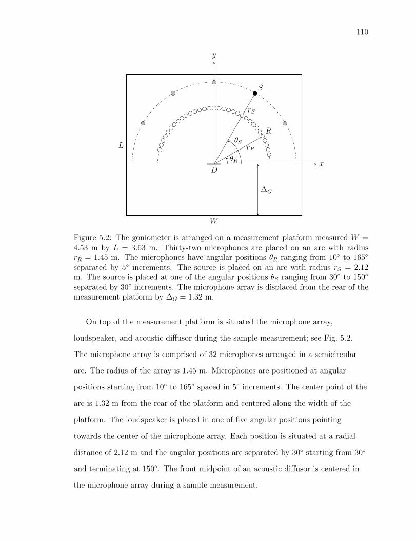
110
x
y
W
L
∆G
D
rS
θSrR
θR
S
R
Figure 5.2: The goniometer is arranged on a measurement platform measured W =4.53 m by L = 3.63 m. Thirty-two microphones are placed on an arc with radiusrR = 1.45 m. The microphones have angular positions θR ranging from 10 to 165
separated by 5 increments. The source is placed on an arc with radius rS = 2.12m. The source is placed at one of the angular positions θS ranging from 30 to 150
separated by 30 increments. The microphone array is displaced from the rear of themeasurement platform by ∆G = 1.32 m.
On top of the measurement platform is situated the microphone array,
loudspeaker, and acoustic diffusor during the sample measurement; see Fig. 5.2.
The microphone array is comprised of 32 microphones arranged in a semicircular
arc. The radius of the array is 1.45 m. Microphones are positioned at angular
positions starting from 10 to 165 spaced in 5 increments. The center point of the
arc is 1.32 m from the rear of the platform and centered along the width of the
platform. The loudspeaker is placed in one of five angular positions pointing
towards the center of the microphone array. Each position is situated at a radial
distance of 2.12 m and the angular positions are separated by 30 starting from 30
and terminating at 150. The front midpoint of an acoustic diffusor is centered in
the microphone array during a sample measurement.

111
5.2.2 Quasi-anechoic Conditions
As mentioned in Sec. 5.1.1 it is important that the scattered signal be conducted
under quasi-anechoic conditions. A quasi-anechoic condition is satisfied if the
scattered signal is captured in a time window free of direct sound and room
reflections. The concept of applying a quasi-anechoic measurement for acoustic
diffusors was pioneered by D’Antonio and Konnert (D’Antonio and Konnert, 1992).
The original conception of a quasi-anechoic measurement is based upon an
equivalent idea called the reflection free zone (Cox and D’Antonio, 2009, pp. 113,
114). Ideally, direct sound precedes the onset of the scattered signal by two
milliseconds and room reflections proceeds the onset of the scattered signal by two
milliseconds. The original goniometer geometry could not sufficiently separate the
direct and scattered signals for large scattering angles (D’Antonio and Konnert,
1992). By a process of refinement and lately through numerical optimization the
geometric configuration of the goniometer evolved to the present configuration
shown in Fig. 5.2 (D’Antonio and Rife, 2011).
The quasi-anechoic conditions are analyzed by geometric considerations. The
quasi-anechoic boundary is a surface in space beyond which room reflections occur
two milliseconds after the onset of the scattered signal. Each source to microphone
has a different quasi-anechoic boundary. The derivation of the geometric parameters
for each quasi-anechoic boundary is based upon Fig. 5.3. It is understood that a
source S has the polar coordinates (rS, θS), and a receiver R has the polar
coordinates (rR, θR). A coordinate system is established with its origin at the center
of the microphone array. In a sample measurement a diffusor D is placed at the
origin. It can be assumed that the onset of the scattered signal occurs along a path
from S to D and then D to R, which is denoted as−−−→SDR. In order to determine the
quasi-anechoic boundary, it is desired to first compute the corresponding elliptical
parameters associated with the path−−−→SDR. It is recognized that the foci of the

112
ellipse are S and R. The focal length is denoted as f where twice the focal length is
equal to the distance between S and R, |−→SR| = 2f . The center of the ellipse C is
the midpoint of the path−→SR. The interior angle associated with ∠SDR is denoted
as α. The interior angle is computed as the absolute difference between θR and θS,
α = |θR − θS|. (5.12)
By the law of sines the interior angle of ∠DSR is computed as,
β = arcsin[rR sin(α)/2f ], (5.13)
where β = ∠DSR. The rotation angle of the ellipse is computed as,
γ =
θS − β if θR − θS ≥ 0,
θS + β if θR − θS < 0.
(5.14)
By the properties of ellipsis the major and minor axis of the ellipse, which
correspond to the rotated and translated coordinate system at C, are computed as,
a =rS + rR
2, (5.15)
b =√a2 − f 2, (5.16)
where a and b are the lengths of the major and minor axis of the ellipse, respectively.
The ellipse with the parameters computed from Eqs. (5.14)–(5.16) is shown as a
black dashed ellipse in Fig. 5.3. In a large part the generated ellipse is dependent
upon the path lengths from the source to diffusor and diffusor to receiver. In a like
manner the quasi-anechoic boundary is based upon the path lengths from the source

113
to diffusor, diffusor to receiver, and a buffer distance based upon the buffer time,
d = cτ, (5.17)
where d is the buffer distance, c is the speed of sound, and τ is the buffer time (4
ms). The buffer time allows for time spreading due to surface scattering and an
allowance for a time window free of reflections. The major axis and minor axis of
the quasi-anechoic boundary is computed similarly to Eqs. (5.15) and (5.16) by
considering the buffer distance,
aQA =rS + rR + d
2, (5.18)
bQA =√a2QA − f 2, (5.19)
where aQA and bQA are the lengths of the major and minor axis of the
quasi-anechoic boundary ellipse, respectively. It is important to note that the total
quasi-anechoic boundary is a hemiellipsoid generated as a surface of revolution
about the elliptical major axis. The quasi-anechoic boundary is denoted as a red
dashed ellipse in Fig. 5.3. Thus, for no room reflections to occur within the buffer
time window after the onset of scattering, no reflecting surfaces besides the diffusor
can exist within the hemiellipsoid of the quasi-anechoic boundary. Another
consideration is the time separation between the direct sound and the onset of
scattering. The time separation is based upon the difference in the path lengths−→SR
and−−−→SDR. In general the buffer time of two milliseconds is satisfied by the
goniometer configuration; however for some particular source and receiver angles the
path length difference corresponds to less than the buffer time. For example, given a
source position at 30 and a receiver at 165 the path length difference is 0.262 m,
which is a 0.76 ms time difference between the direct and scattered sound.

114
x
y
D
Cx′
y′rS
rRα
θR θS
β
γS
R
Figure 5.3: Quasi-anechoic conditions for the sample measurement. Geometry forthe derivation of the quasi-anechoic boundary. The goniometer measurement consistsof a diffusor located at D, one receiver of 32 shown as R, and the source S. Thequasi-anechoic boundary, denoted as a dashed red ellipse, defines the extent of soundpropagation from S, to a room reflection, and then to R two milliseconds after the on-
set of the scattered response (−−−→SDR). The quasi-anechoic boundary is a hemiellipsoid
in three-dimensional space being a surface of revolution about the major axis with acenter at C. The hemiellipsoid has foci at S and R. The positions of the source andreceiver are defined in terms of polar coordinates (rS, θS), and (rR, θR), respectively.

115
For room reflections to be delayed in time sufficiently ahead the onset of
scattering, a clear distance must exist around and above the goniometer. Analysis of
the quasi-anechoic boundary leads to the conclusion that the hemiellipsoid is largest
when θR = θS. By Eq. (5.18) the major axis of the hemiellipsoid does not change,
since the buffer distance and the radii of the source and receivers are constant.
However, the minor axis of the hemiellipsoid changes based on a varying focal
length; see Eq. (5.19). The focal length is a minimum when θR = θS. In the
horizontal plane the quasi-anechoic boundary is shown in Fig. 5.4. Around the
measurement platform exists a clear strip of space that is 1.37 m wide. In general
this clear space prevents any room reflections from reaching the receiver within the
buffer time. Vertically, the quasi-anechoic boundary extends to a maximum height
equal to the minor axis of the ellipse, see Eq. (5.19). The height of the measurement
room is 2.43 m and the maximum length of the minor axis is 2.40 m. Thus, the
measurement room is sufficiently large to facilitate a quasi-anechoic measurement.
5.2.3 Excitation Signals
Two excitation signals are used with the goniometer. The traditional MLS is a 17th
order signal that is pre-emphasized. The signal was generated by the software
EASERA version 1.2 (GmbH, 2012, p. 32). The transition frequency of the
pre-emphasized MLS is approximately 350 Hz where the lower frequencies are
emphasized relative to the higher frequencies. Since the MLS is a 17th order signal
by Eq. (5.10) the signal has a length of 131071 samples. At a sampling frequency of
48 kHz this translates into a signal duration of 2.73 seconds. The energy density
spectrum of the MLS is shown in Fig. 5.5. The second excitation signal is a LSS.
The signal length is comparable to the length of the MLS. The signal has a length
of 131072 (217) samples. The initial sweep frequency is 80 Hz and the final sweep
frequency is 24 kHz. The signal is filtered by a second-order Butterworth filter with

116
x
y
W
L
∆
∆G
D
Cx′ y′
rS
rR
θR
θS
S
R
Figure 5.4: The quasi-anechoic boundary is largest when θR = θS. Here the goniome-ter is shown in the context of the measurement platform and a strip of free spacesurrounding the platform. The measurement platform has the following dimensions:W = 4.53 m by L = 3.63 m. The microphone array is displaced from the rear of themeasurement platform by ∆G = 1.32 m and the strip of free space has a constantwidth of ∆ = 1.37 m. The walls of the measurement room are outside the strip offree space.
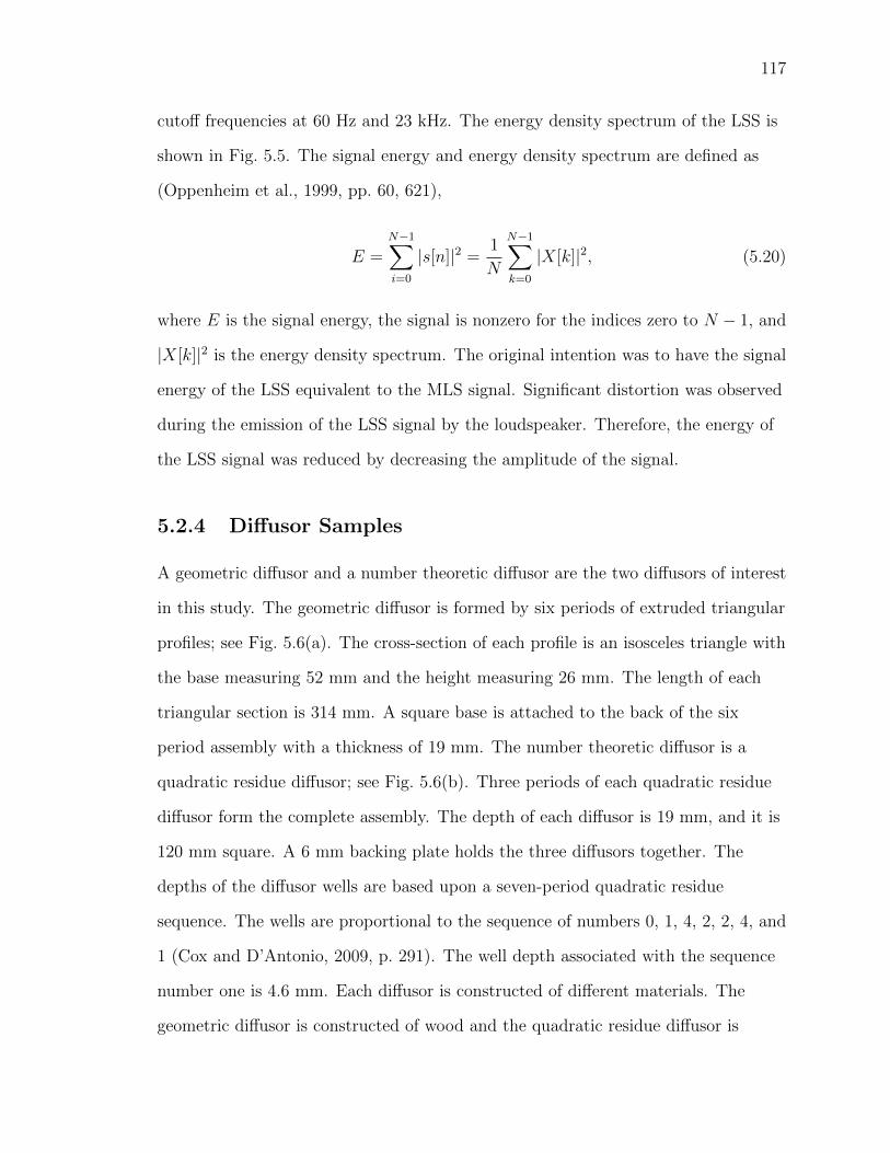
117
cutoff frequencies at 60 Hz and 23 kHz. The energy density spectrum of the LSS is
shown in Fig. 5.5. The signal energy and energy density spectrum are defined as
(Oppenheim et al., 1999, pp. 60, 621),
E =N−1∑i=0
|s[n]|2 =1
N
N−1∑k=0
|X[k]|2, (5.20)
where E is the signal energy, the signal is nonzero for the indices zero to N − 1, and
|X[k]|2 is the energy density spectrum. The original intention was to have the signal
energy of the LSS equivalent to the MLS signal. Significant distortion was observed
during the emission of the LSS signal by the loudspeaker. Therefore, the energy of
the LSS signal was reduced by decreasing the amplitude of the signal.
5.2.4 Diffusor Samples
A geometric diffusor and a number theoretic diffusor are the two diffusors of interest
in this study. The geometric diffusor is formed by six periods of extruded triangular
profiles; see Fig. 5.6(a). The cross-section of each profile is an isosceles triangle with
the base measuring 52 mm and the height measuring 26 mm. The length of each
triangular section is 314 mm. A square base is attached to the back of the six
period assembly with a thickness of 19 mm. The number theoretic diffusor is a
quadratic residue diffusor; see Fig. 5.6(b). Three periods of each quadratic residue
diffusor form the complete assembly. The depth of each diffusor is 19 mm, and it is
120 mm square. A 6 mm backing plate holds the three diffusors together. The
depths of the diffusor wells are based upon a seven-period quadratic residue
sequence. The wells are proportional to the sequence of numbers 0, 1, 4, 2, 2, 4, and
1 (Cox and D’Antonio, 2009, p. 291). The well depth associated with the sequence
number one is 4.6 mm. Each diffusor is constructed of different materials. The
geometric diffusor is constructed of wood and the quadratic residue diffusor is

118
102 103 10430
35
40
45
50
55
60
Frequency [Hz]
Ener
gyD
ensi
tySp
ectr
um
[dB
]
Figure 5.5: The energy density spectrum of a logarithmic swept-sine signal (graycurve) and a maximum length sequence signal (black curve).
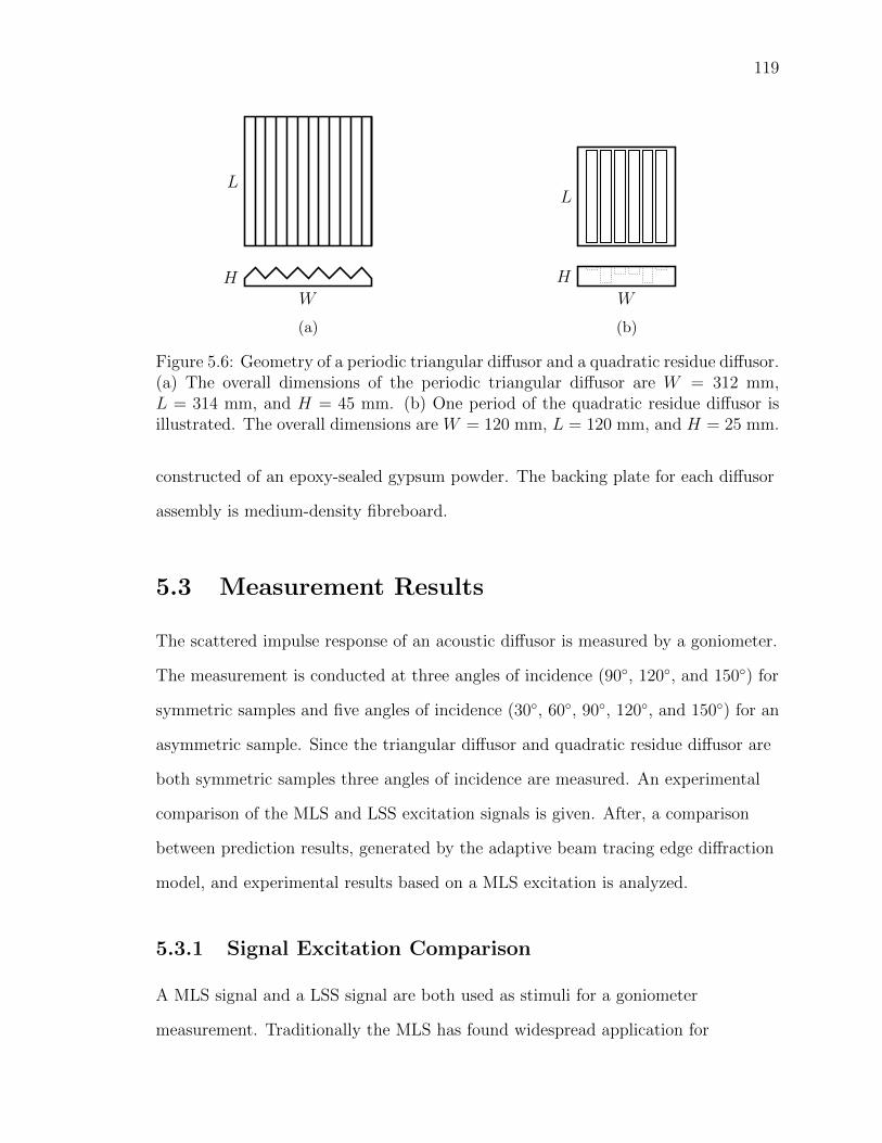
119
HW
L
(a)
H
W
L
(b)
Figure 5.6: Geometry of a periodic triangular diffusor and a quadratic residue diffusor.(a) The overall dimensions of the periodic triangular diffusor are W = 312 mm,L = 314 mm, and H = 45 mm. (b) One period of the quadratic residue diffusor isillustrated. The overall dimensions are W = 120 mm, L = 120 mm, and H = 25 mm.
constructed of an epoxy-sealed gypsum powder. The backing plate for each diffusor
assembly is medium-density fibreboard.
5.3 Measurement Results
The scattered impulse response of an acoustic diffusor is measured by a goniometer.
The measurement is conducted at three angles of incidence (90, 120, and 150) for
symmetric samples and five angles of incidence (30, 60, 90, 120, and 150) for an
asymmetric sample. Since the triangular diffusor and quadratic residue diffusor are
both symmetric samples three angles of incidence are measured. An experimental
comparison of the MLS and LSS excitation signals is given. After, a comparison
between prediction results, generated by the adaptive beam tracing edge diffraction
model, and experimental results based on a MLS excitation is analyzed.
5.3.1 Signal Excitation Comparison
A MLS signal and a LSS signal are both used as stimuli for a goniometer
measurement. Traditionally the MLS has found widespread application for
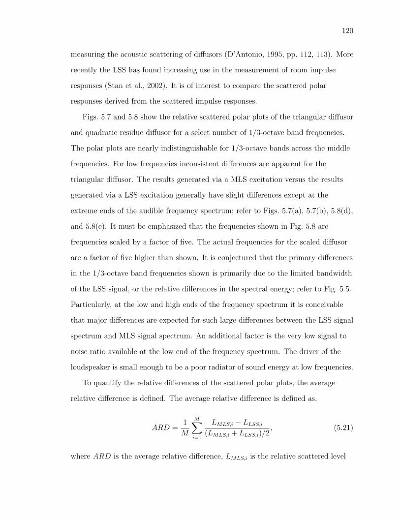
120
measuring the acoustic scattering of diffusors (D’Antonio, 1995, pp. 112, 113). More
recently the LSS has found increasing use in the measurement of room impulse
responses (Stan et al., 2002). It is of interest to compare the scattered polar
responses derived from the scattered impulse responses.
Figs. 5.7 and 5.8 show the relative scattered polar plots of the triangular diffusor
and quadratic residue diffusor for a select number of 1/3-octave band frequencies.
The polar plots are nearly indistinguishable for 1/3-octave bands across the middle
frequencies. For low frequencies inconsistent differences are apparent for the
triangular diffusor. The results generated via a MLS excitation versus the results
generated via a LSS excitation generally have slight differences except at the
extreme ends of the audible frequency spectrum; refer to Figs. 5.7(a), 5.7(b), 5.8(d),
and 5.8(e). It must be emphasized that the frequencies shown in Fig. 5.8 are
frequencies scaled by a factor of five. The actual frequencies for the scaled diffusor
are a factor of five higher than shown. It is conjectured that the primary differences
in the 1/3-octave band frequencies shown is primarily due to the limited bandwidth
of the LSS signal, or the relative differences in the spectral energy; refer to Fig. 5.5.
Particularly, at the low and high ends of the frequency spectrum it is conceivable
that major differences are expected for such large differences between the LSS signal
spectrum and MLS signal spectrum. An additional factor is the very low signal to
noise ratio available at the low end of the frequency spectrum. The driver of the
loudspeaker is small enough to be a poor radiator of sound energy at low frequencies.
To quantify the relative differences of the scattered polar plots, the average
relative difference is defined. The average relative difference is defined as,
ARD =1
M
M∑i=1
LMLS,i − LLSS,i(LMLS,i + LLSS,i)/2
, (5.21)
where ARD is the average relative difference, LMLS,i is the relative scattered level

121
0
30
6090
120
150
1800 20 40
[dB]
(a) 315 Hz
0
30
6090
120
150
1800 20 40
[dB]
(b) 400 Hz
0
30
6090
120
150
1800 20 40
[dB]
(c) 1000 Hz
0
30
6090
120
150
1800 20 40
[dB]
(d) 1250 Hz
0
30
6090
120
150
1800 20 40
[dB]
(e) 3150 Hz
0
30
6090
120
150
1800 20 40
[dB]
(f) 4000 Hz
Figure 5.7: Experimental relative scattered levels for a triangular diffusor are com-pared between a MLS signal (black curve) and a LSS signal (gray curve). The sourceis incident from a polar angle of 30. One-third octave band results are shown in (a)through (f).
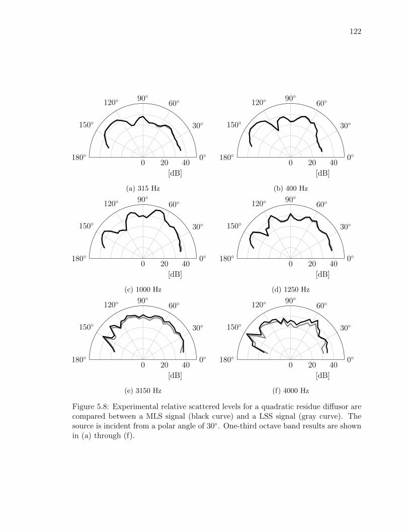
122
0
30
6090
120
150
1800 20 40
[dB]
(a) 315 Hz
0
30
6090
120
150
1800 20 40
[dB]
(b) 400 Hz
0
30
6090
120
150
1800 20 40
[dB]
(c) 1000 Hz
0
30
6090
120
150
1800 20 40
[dB]
(d) 1250 Hz
0
30
6090
120
150
1800 20 40
[dB]
(e) 3150 Hz
0
30
6090
120
150
1800 20 40
[dB]
(f) 4000 Hz
Figure 5.8: Experimental relative scattered levels for a quadratic residue diffusor arecompared between a MLS signal (black curve) and a LSS signal (gray curve). Thesource is incident from a polar angle of 30. One-third octave band results are shownin (a) through (f).

123
at a specific 1/3-octave band frequency and receiver position for a MLS signal
excitation, LLSS,i is the relative scattered level at a specific 1/3-octave band
frequency and receiver position for a LSS signal excitation, and M is the total
number of receivers (32 in this case). Tables 5.1 and 5.2 show the average relative
difference of the scattering by a triangular diffusor and the quadratic residue
diffusor, respectively. Three columns are tabulated for source angles of incidence
30, 60, and 90. The 100 Hz 1/3-octave band, in Table 5.1, shows a large
inconsistency across the source angles of incidence. A possible source for this
inconsistency is an increase of background noise stemming from mechanical building
HVAC equipment. In contrast, from 125 Hz and upwards the average relative
differences are fairly consistent across the three source angles of incidence. From 125
Hz and upward the average relative difference diminishes for increasing frequency
eventually leveling off. Unlike the triangular diffusor the average relative difference
increases as the frequency increases for the quadratic residue diffusor; refer to Table
5.2. In spite of the contradictory trends in the average relative difference, the polar
plots in Figs. 5.7 and 5.8 indicate a scaling error at high frequencies for the
quadratic residue diffusor and a low signal to noise ratio at the low frequency for the
triangular diffusor. Despite the LSS signal having less signal energy, as defined by
Eq. (5.20) and compared to the MLS signal, a good agreement exists between the
relative scattered levels derived by either excitation signal.
5.3.2 Prediction and Measurement Comparison
A comparison between the adaptive beam tracing edge diffraction model and the
goniometer measurement of the triangular diffusor tested serves the purpose of
numerical validation. The essential details of the goniometer measurement are
modeled. The geometry of the diffusor, extent of the measurement platform, source
positions, and receiver positions are modeled. The comparison is qualitatively

124
Table 5.1: Average relative difference for relative scattered levels of a triangulardiffusor measured by MLS and LSS.
1/3-Octave Angle of Incidence
Band [Hz] 30 60 90
100 2.38 4.87 2.32125 0.27 0.21 0.37160 0.16 0.12 0.18200 0.14 0.08 0.14250 0.11 0.07 0.10315 0.08 0.06 0.07400 0.05 0.05 0.04500 0.03 0.02 0.03630 0.02 0.02 0.03800 0.02 0.02 0.031000 0.02 0.02 0.031250 0.01 0.02 0.031600 0.02 0.02 0.032000 0.02 0.02 0.032500 0.01 0.02 0.033150 0.01 0.02 0.024000 0.01 0.02 0.035000 0.01 0.03 0.036300 0.02 0.02 0.028000 0.01 0.02 0.0210000 0.01 0.04 0.0212500 0.02 0.02 0.0216000 0.03 0.02 0.0320000 0.03 0.02 0.03
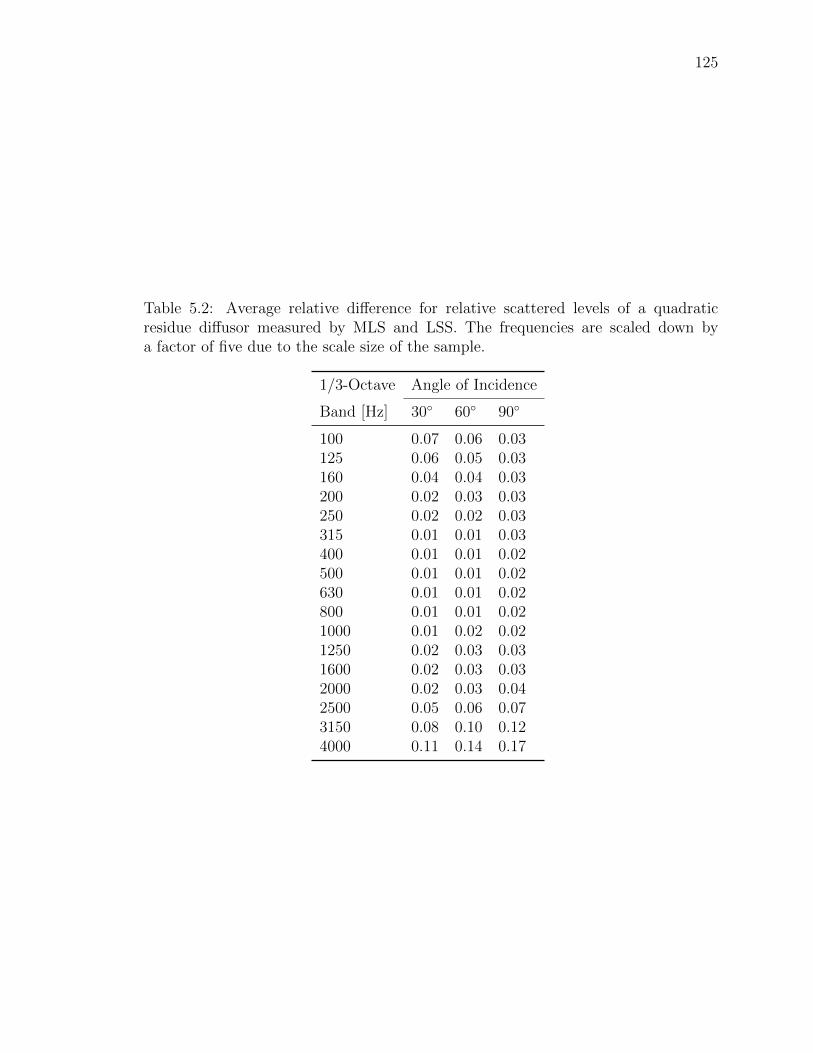
125
Table 5.2: Average relative difference for relative scattered levels of a quadraticresidue diffusor measured by MLS and LSS. The frequencies are scaled down bya factor of five due to the scale size of the sample.
1/3-Octave Angle of Incidence
Band [Hz] 30 60 90
100 0.07 0.06 0.03125 0.06 0.05 0.03160 0.04 0.04 0.03200 0.02 0.03 0.03250 0.02 0.02 0.03315 0.01 0.01 0.03400 0.01 0.01 0.02500 0.01 0.01 0.02630 0.01 0.01 0.02800 0.01 0.01 0.021000 0.01 0.02 0.021250 0.02 0.03 0.031600 0.02 0.03 0.032000 0.02 0.03 0.042500 0.05 0.06 0.073150 0.08 0.10 0.124000 0.11 0.14 0.17

126
analyzed by an examination of the relative scattered level polar plots and the
root-mean-square error between the predicted and measured results.
Figure 5.9 shows the relative scattered levels determined by experiment and
prediction. The source is incident from an angle of 30. Up to second-order
diffraction is computed. The agreement between experiment and prediction is best
at the 4000 Hz 1/3-octave band and gradually declines for lower 1/3-octave band
frequencies. The departure from agreement is attributed to two factors, and
possibly an additional third factor: the increasing importance of higher-order
diffraction, the omission of reflection-diffraction combinations, and diaphragmatic
absorption. Higher-order diffraction plays an essential role in the scattered field for
low frequencies (Chu et al., 2007). In a similar vein the omission of
reflection-diffraction combinations affects the magnitude of the scattered sound
field. For example, the mechanism of wedge diffraction, reflection, and wedge
diffraction is omitted, which may play an essential role in predicting the magnitude
of the scattered sound field accurately at mid-frequencies. Lastly, diaphragmatic
absorption possibly explains the reduced experimental magnitude of the scattered
field at low frequencies (D’Antonio and Konnert, 1992). Since, the prediction
assumes a perfectly rigid surface, no acoustic absorption is accounted for.
The root-mean-square error (RMSE) of the relative scattered levels between the
experimental results and prediction results are tabulated in Table 5.3. The RMSE is
greatest at low frequencies with the exception of 100 Hz, and 125 Hz 1/3-octave
bands. The importance of including higher-order diffraction, and additional
reflection-diffraction combinations is stressed by the high RMSE below 1000 Hz,
which is greater than or equal to 10.0 dB for the 1/3-octave bands 160 Hz to 800
Hz. The magnitude of the RMSE is smaller for 1000 Hz and above, however, the
values do not monotonically decrease to zero as the frequency increases. It is
conjectured that as the frequency increases the directivity of the loudspeaker limits

127
0
30
6090
120
150
1800 20 40
[dB]
(a) 315 Hz
0
30
6090
120
150
1800 20 40
[dB]
(b) 400 Hz
0
30
6090
120
150
1800 20 40
[dB]
(c) 1000 Hz
0
30
6090
120
150
1800 20 40
[dB]
(d) 1250 Hz
0
30
6090
120
150
1800 20 40
[dB]
(e) 3150 Hz
0
30
6090
120
150
1800 20 40
[dB]
(f) 4000 Hz
Figure 5.9: Experimental (black) versus predicted (gray) relative scattered levels fora periodic triangular diffusor. The source is incident from a polar angle of 30. Up tosecond-order diffraction is computed in the prediction. One-third octave band resultsare shown in (a) through (f).
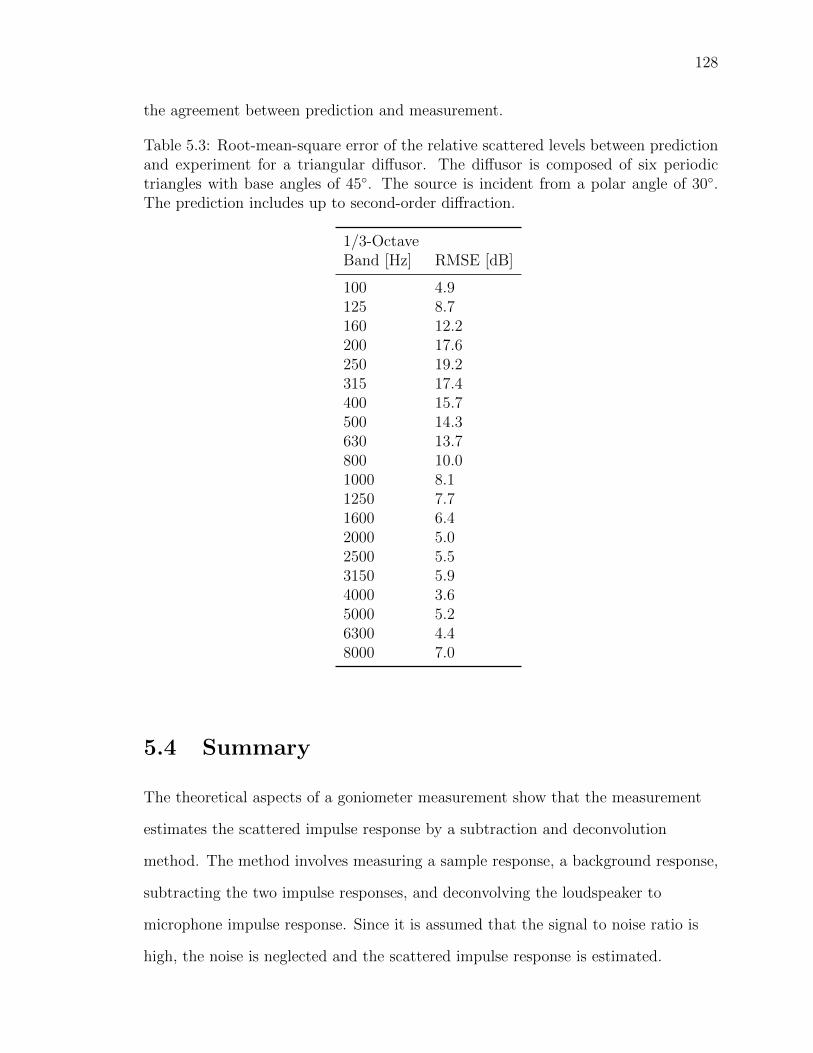
128
the agreement between prediction and measurement.
Table 5.3: Root-mean-square error of the relative scattered levels between predictionand experiment for a triangular diffusor. The diffusor is composed of six periodictriangles with base angles of 45. The source is incident from a polar angle of 30.The prediction includes up to second-order diffraction.
1/3-OctaveBand [Hz] RMSE [dB]
100 4.9125 8.7160 12.2200 17.6250 19.2315 17.4400 15.7500 14.3630 13.7800 10.01000 8.11250 7.71600 6.42000 5.02500 5.53150 5.94000 3.65000 5.26300 4.48000 7.0
5.4 Summary
The theoretical aspects of a goniometer measurement show that the measurement
estimates the scattered impulse response by a subtraction and deconvolution
method. The method involves measuring a sample response, a background response,
subtracting the two impulse responses, and deconvolving the loudspeaker to
microphone impulse response. Since it is assumed that the signal to noise ratio is
high, the noise is neglected and the scattered impulse response is estimated.
129
The goniometer measurement involves various experimental apparatus. The
goniometer itself consists of a measurement platform, a 32 microphone array, and a
loudspeaker. The microphone array is powered by a bank of four preamplifiers in a
master-slave setup, and the loudspeaker is powered by a power amplifier. The power
amplifier is connected to the master preamplifier and the four preamplifiers are
connected to a measurement desktop. Physical considerations are taken into
account for the purpose of conducting a measurement in a quasi-anechoic condition.
It is verified that quasi-anechoic conditions are present during a measurement with
the exception of a few source and receiver angles.
Measurement of acoustic scattering by a geometric diffusor and a number
theoretic diffusor is conducted with two types of excitation signals. The MLS and
LSS excitation signals are compared in a relative sense for the relative scattered
levels derived from the measurement. In spite of containing less energy the
employed LSS signal resulted in measurements that agree very well with the MLS
measurements over several 1/3-octave band frequencies. The largest relative
differences are for low frequencies. Finally, a numerical validation of the prediction
model, developed in this dissertation, is conducted with the result that predictions
are best suited for high frequencies.

Chapter 6
Conclusions
The purpose of the present study is to investigate the capabilities and limitations of
a combined adaptive tetrahedral tracing and edge diffraction model. The case study
of interest is the prediction of scattering by diffusors. Viewing an acoustic diffusor
as an ensemble of finite reflective surfaces comprised of scattering wedges leads to a
particularly useful approach. Three challenges exist in the realization of this
modeling approach. The first challenge is determining, and if applicable defining,
the geometric acoustics model appropriate for diffusor scattering predictions. The
second challenge is to identify and define an interface between the geometric
acoustic model and a edge scattering model. Lastly, the third challenge is to
numerically verify, and validate the proposed approach.
6.1 General Conclusions
The first research challenge is to identify, and if necessary define, a relevant
geometric acoustics model for the combined model. Of the available techniques, the
adaptive beam tracing model shows the greatest promise since it maps the incident
and reflected sound fields in a continuous manner. The advantage of mapping the
incident and reflected sound fields continuously is evident by the capability to
130
131
identify scattering wedge parameters. The relevant literature on acoustic adaptive
beam tracing omits several algorithmic aspects crucial for the physically correct
mapping of incident and reflected sound fields. Upon further investigation the
necessary elements were derived for the model and the algorithm termed adaptive
tetrahedral tracing. The fundamental algorithmic procedures include ensonification
mapping, occlusion mapping, and the subdivision of the total ensonification
mapping (for further details see Sec. 3.2). An added advantage of adaptive
tetrahedral tracing is the ability to map the incident and reflected sound fields on
the boundaries of the geometric domain. This characteristic establishes a vital
interface for an edge scattering model.
The second challenge is to identify and define an interface between the geometric
acoustic model and an edge scattering model. The adaptive tetrahedral tracing
algorithm maps the incident and reflected acoustic sound fields on the boundaries of
the geometric domain. Once the mapping is established a system identifies the
diffracting edges. The parameters of each scattering wedge are extracted from the
acoustic mapping and funneled to the edge scattering model. Geometric parameters
such as the wedge angle, relative cylindrical coordinates of the source and receiver,
and extent of the ensonified edge are extracted from the acoustic mapping.
Higher-order diffraction is treated from the perspective of graph-theory.
Permutations of reflection and diffraction are enumerated through modified
graph-theoretic search procedures. Details are provided in Secs. 4.1 through 4.3.
The third and final challenge is to numerically verify, and validate the combined
adaptive tetrahedral tracing edge diffraction model. The model is numerically
verified against three scattering geometries. Overall the agreement against analytic
and boundary element predictions (BEM) predictions is good. It is determined that
as the geometry of the diffusor becomes more complex, then a greater need for
higher-order diffraction and additional diffraction-reflection permutations are

132
necessary to correctly model wave propagation at low frequencies; see Sec. 4.4.
Numerical validation is conducted against goniometer measurements of two
geometric diffusors. The resulting comparisons between prediction and experimental
results suggests that the model requires higher-order diffraction and additional
diffraction-reflection permutations for broadband predictions; see Sec. 5.3.2.
Additionally, part of the experimental portion involves an investigation into
measurements with two different stimuli. Traditionally the maximum length
sequence (MLS) is used most widely in the measurement of acoustic diffusors. It is
of interest to examine an alternative stimuli, specifically the logarithmic swept-sine
(LSS). The choice of a LSS stimuli is motivated by the fact that the method rejects
harmonic distortion, and is capable of conducting measurements at a higher signal
to noise ratio. Measurements of acoustic diffusors show that the LSS stimuli is an
acceptable signal type since very good agreement exists for the scattered polar
responses over a large frequency range when compared against measurements with
MLS stimuli; see Sec. 5.3.1.
6.2 Present Challenges and Opportunities
Several opportunities are available to extend the adaptive tetrahedral tracing and
edge diffraction model. One particular challenge is to dynamically identify geometry
that would otherwise go undetected by the model; see Fig. 3.1(b) for an example.
Small geometric features relative to the propagating tetrahedral cross-section result
in one type of acoustic aliasing. Drumm and Lam (2000) claim that their algorithm
identifies geometric features wholly contained within a beam, but no substantial
details exist on how to dynamically identify such a scenario. The solution proposed
in this study is to increase the beam density ensuring that this type of acoustic
aliasing is avoided. However, this solution is far from ideal since it is based on a

133
trial and error process.
Another challenge is to model additional reflection-diffraction permutations. For
example, the inclusion of diffraction, reflection, and diffraction combinations may
improve the agreement between predictions and experiment. The challenge of
computing such combinations includes modeling image edges instead of image
source, and computing from region visibility (Antani et al., 2012). In the present
study it is assumed that mutually visible edges are completely visible to one
another. A from region visibility computation where the mutual visibility of edges
are considered would correct that assumption. Furthermore, the secondary source
model for edge diffraction does not account for slope diffraction (Summers, 2013).
Slope diffraction is an important component of the sound field generated by wave
guides (Mentzer et al., 1975). The quadratic residue diffusor and other diffusors
that exhibit semi-enclosed volumes act as acoustic wave guides. Current models
that compute electromagnetic slope diffraction in the time-domain may be
applicable to sound propagation (Rousseau and Pathak, 1995).
Geometric domains that contain many polygons present a particular
computational bottleneck for naive ray-polygon intersection queries. Approximately
only half of the polygons are discarded based on the directional vector of the ray
and each polygon normal. A major improvement to the adaptive tetrahedral tracing
algorithm is accelerating ray-polygon intersection tests. The most notable
techniques for accelerating ray-polygon intersection queries are kd-tree traversal and
binary space partitioning. Binary space partitioning is used by Funkhouser et
al. (2004) in a beam tracing algorithm for purpose of computing real-time
auralizations. Binary space partitioning splits the geometric domain into convex
parallelepipeds and constrains the query space to a subset of the total geometric
domain. Another technique well-suited to adaptive tetrahedral tracing is kd-tree
traversal (Overbeck et al., 2007; Hapala and Havran, 2011). Similar to binary-space

134
partitioning the geometric domain is split into cells that subdivide the geometric
domain, which accelerates the ray-polygon query.
Lastly, modeling acoustic impedance in the time-domain is a current challenge
with some approaches suggested within the literature. Going beyond rigid or
anechoic boundaries requires special considerations: for example, how to model the
multiple convolutions that physically occur during beam-boundary interactions.
Work applied to the finite difference time-domain method (Kowalczyk and van
Walstijn, 2008a,b) may find application with adaptive tetrahedral tracing. Plus,
diffraction of general impedance wedges is as of now an open problem. The closest
solution was developed for an isovelocity wedge with varying densities (Chu, 1989).
Bibliography
AES Standards Committee. Aes information document for room acoustics and
sound reinforcement systems - characterisation and measurement of surface
scattering uniformity. Technical Report AES-4id-2001 (r2007), Audio Engineering
Society, Inc., 2001.
Jont B. Allen and David A. Berkley. Image method for efficiently simulating
small-room acoustics. The Journal of the Acoustical Society of America, 65(4):
943–950, 1979.
Lakulish Antani, Anish Chandak, Micah Taylor, and Dinesh Manocha. Efficient
finite-edge diffraction using conservative from-region visibility. Applied Acoustics,
73(3):218–233, 2012.
Andreas Asheim and U. Peter Svensson. An integral equation formulation for the
diffraction from convex plates and polyhedra. The Journal of the Acoustical
Society of America, 133(6):3681–3691, June 2013 2013.
Keith Attenborough, Kai Ming Li, and Kirill Horoshenkov. Predicting outdoor
sound. Taylor & Francis, London ; New York, 2007.
Jørgen Bang-Jensen and Gregory Gutin. Digraphs: theory, algorithms, and
applications. Springer, London ; New York, 2001.
Imran Bashir, Shahram Taherzadeh, and Keith Attenborough. Diffraction assisted
135

136
rough ground effect: Models and data. The Journal of the Acoustical Society of
America, 133(3):1281–1292, 2013.
John R. Berryhill. Diffraction response for nonzero separation of source and
receiver. Geophysics, 42(6):1158–1176, 1977.
David A. Bies and Colin H. Hansen. Engineering noise control: theory and pratice.
Spon Press/Taylor & Francis, London ; New York, 4th edition, 2009.
M. A. Biot. Reflection on a rough surface from an acoustic point source. The
Journal of the Acoustical Society of America, 29(11):1193–1200, 1957.
M. A. Biot and I. Tolstoy. Formulation of wave propagation in infinite media by
normal coordinates with an application to diffraction. The Journal of the
Acoustical Society of America, 29(3):381–391, 1957.
D. Botteldooren. Acoustical finite-difference time-domain simulation in a
quasi-cartesian grid. The Journal of the Acoustical Society of America, 95(5):
2313–2319, 1994.
Patrice Boulanger, Keith Attenborough, Shahram Taherzadeh, Tim Waters-Fuller,
and Kai Ming Li. Ground effect over hard rough surfaces. The Journal of the
Acoustical Society of America, 104(3):1474–1482, 1998.
J. J. Bowman, Thomas B. A. Senior, P. L. E. Uslenghi, and J. S. Asvestas.
Electromagnetic and acoustic scattering by simple shapes. Hemisphere Pub. Corp.,
New York, rev print edition, 1987.
T. J. I’A Bromwich. Diffraction of waves by a wedge. Proceedings of the London
Mathematical Society, 14(1):450–463, 1915.
A. J. Burton and G. F. Miller. The application of integral equation methods to the
numerical solution of some exterior boundary-value problems. Proceedings of the

137
Royal Society of London.Series A, Mathematical and Physical Sciences, 323
(1553):201–210, 1971.
Nicola Campo, Paolo Rissone, and Marco Toderi. Adaptive pyramid tracing: a new
technique for room acoustics. Applied Acoustics, 61(2):199–221, 2000.
H. S. Carslaw. Diffraction of waves by a wedge of any angle. Proceedings of the
London Mathematical Society, s2-18(1):291–306, 1920.
Dezhang Chu. Impulse response of density contrast wedge using normal coordinates.
The Journal of the Acoustical Society of America, 86(5):1883–1896, 1989.
Dezhang Chu, Timothy K. Stanton, and Allan D. Pierce. Higher-order acoustic
diffraction by edges of finite thickness. The Journal of the Acoustical Society of
America, 122(6):3177–3194, 2007.
C. S. Clay and Wayne A. Kinney. Numerical computations of time-domain
diffractions from wedges and reflections from facets. The Journal of the Acoustical
Society of America, 83(6):2126–2133, 1988.
D. Cohen-Or, Y. L. Chrysanthou, C. T. Silva, and F. Durand. A survey of visibility
for walkthrough applications. Visualization and Computer Graphics, IEEE
Transactions, 9(3):412, 2003.
Thomas H. Cormen, Charles E. Leiserson, Ronald L. Rivest, and Clifford Stein.
Introduction to algorithms. The MIT Press, Cambridge Massachusetts ; London, 3
edition, 2009.
T. Cox and Y. W. Lam. Prediction and evaluation of the scattering from quadratic
residue diffusers. The Journal of the Acoustical Society of America, 95(1):297–9,
1994.

138
Trevor J. Cox. The optimization of profiled diffusers. The Journal of the Acoustical
Society of America, 97(5):2928–2936, 1995.
Trevor J. Cox and Peter D’Antonio. Acoustic absorbers and diffusers: theory, design
and application. Taylor & Francis, London ; New York, 2 edition, 2009.
Trevor J. Cox and Peter D’Antonio. Acoustic surface reflection database, 2011.
Konstantinos Dadiotis, Jamie A. S. Angus, and Trevor J. Cox. Luke and power
residue sequence diffusers. The Journal of the Acoustical Society of America, 123
(4):2035–2042, 2008.
Norm Dadoun, David G. Kirkpatrick, and John P. Walsh. The geometry of beam
tracing. In SCG ’85: Proceedings of the first annual symposium on Computational
geometry, pages 55–61, New York, NY, USA, 1985. ACM.
Bengt-Inge L. Dalenback. Room acoustic prediction based on a unified treatment of
diffuse and specular reflection. The Journal of the Acoustical Society of America,
100(2):899–909, 1996.
Peter D’Antonio. Performance evaluation of optimized diffusors. The Journal of the
Acoustical Society of America, 97(5):2937–2941, 1995.
Peter D’Antonio and John Konnert. The directional scattering coefficient:
Experimental determination. J. Audio Eng. Soc., 40(12):997–1017, 1992.
Peter D’Antonio and Brian Rife. The state of the art in the measurement of
acoustical coefficients. volume 12, page 015008. ASA, 2011.
I. A. Drumm. The application of adaptive beam tracing and managed directx for
the visualisation and auralisation of virtual environments. In Information
Visualisation, 2005. Proceedings. Ninth International Conference, pages 961–965,
2005.
139
I. A. Drumm and Y. W. Lam. The adaptive beam-tracing algorithm. Journal of the
Acoustical Society of America, 107(3):1405–1412, 2000.
Jose Escolano, Finn Jacobsen, and Jose J. Lopez. An efficient realization of
frequency dependent boundary conditions in an acoustic finite-difference
time-domain model. Journal of Sound and Vibration, 316(15):234–247, 2008.
Angelo Farina. Simultaneous measurement of impulse response and distortion with
a swept-sine technique. 2000.
T. Funkhouser, N. Tsingos, I. Carlbom, G. Elko, M. Sondhi, J. E. West, G. Pingali,
P. Min, and A. Ngan. A beam tracing method for interactive architectural
acoustics. Journal of the Acoustical Society of America, 115(2):739–756, 2004.
W. Gander and W. Gautschi. Adaptive quadrature - revisited. BIT, 40(1):84–101,
2000.
Dan Givoli. Numerical methods for problems in infinite domains, volume 33.
Elsevier, Amsterdam, 1992.
AFMG Technologies GmbH. Easera tutorial. Technical Report EASERA 1.2,
AFMG Technologies GmbH, 2012.
Oriol Guasch and Lluis Cortes. Graph theory applied to noise and vibration control
in statistical energy analysis models. The Journal of the Acoustical Society of
America, 125(6):3657–3672, 2009.
W. James Hadden, Jr. and Allan D. Pierce. Sound diffraction around screens and
wedges for arbitrary point source locations. The Journal of the Acoustical Society
of America, 69(5):1266–1276, 1981.
Thorkild Hansen and Arthur D. Yaghjian. Plane-wave theory of time-domain fields:
near-field scanning applications. IEEE Press, New York, NY, 1999.

140
M. Hapala and V. Havran. Review: Kd-tree traversal algorithms for ray tracing.
Computer Graphics Forum, 30(1):199–213, 2011.
Jonathan A. Hargreaves and Trevor J. Cox. A transient boundary element method
model of schroeder diffuser scattering using well mouth impedance. The Journal
of the Acoustical Society of America, 124(5):2942–2951, 2008.
T. Hargreaves, T. Cox, Y. Lam, and P. D’Antonio. Surface diffusion coefficients for
room acoustics: Free-field measures. The Journal of the Acoustical Society of
America, 108(4):1710–1720, 2000.
M. H. Hayes. Statistical digital signal processing and modeling. John Wiley & Sons,
New York, 1996.
Paul S. Heckbert and Pat Hanrahan. Beam tracing polygonal objects. In
SIGGRAPH ’84: Proceedings of the 11th annual conference on Computer graphics
and interactive techniques, pages 119–127, New York, NY, USA, 1984. ACM.
K. Ito. Encyclopedic Dictionary of Mathematics: The Mathematical Society of
Japan, volume 1. MIT Press, 1993.
Cheol-Ho Jeong. Absorption and impedance boundary conditions for phased
geometrical-acoustics methods. The Journal of the Acoustical Society of America,
132(4):2347–2358, 2012.
Wayne A. Kinney, C. S. Clay, and Gerald A. Sandness. Scattering from a
corrugated surface: Comparison between experiment, helmholtz–kirchhoff theory,
and the facet-ensemble method. The Journal of the Acoustical Society of
America, 73(1):183–194, 1983.
Lawrence E. Kinsler, Austin R. Frey, Alan B. Coppens, and James V. Sanders.
Fundamentals of acoustics. Usa, John Wiley & Sons. Inc., fourth edition, 2000.

141
R. G. Kouyoumjian and P. H. Pathak. A uniform geometrical theory of diffraction
for an edge in a perfectly conducting surface. Proceedings of the IEEE, 62(11):
1448, 1974.
Konrad Kowalczyk and Maarten van Walstijn. Modeling frequency-dependent
boundaries as digital impedance filters in fdtd and k-dwm room acoustics
simulations. J.Audio Eng.Soc, 56(7/8):569–583, 2008a.
Konrad Kowalczyk and Maarten van Walstijn. Formulation of locally reacting
surfaces in fdtd/k-dwm modelling of acoustic spaces. Acta Acustica united with
Acustica, 94(6):891–906, 2008b.
Andrzej Kulowski. Algorithmic representation of the ray tracing technique. Applied
Acoustics, 18(6):449–469, 1985.
T. I. Laakso, V. Valimaki, M. Karjalainen, and U. K. Laine. Splitting the unit delay
[fir/all pass filters design]. Signal Processing Magazine, IEEE, 13(1):30–60, 1996.
H. Lehnert. Systematic-errors of the ray-tracing algorithm. Applied Acoustics, 38
(2-4):207–221, 1993.
T. Lewers. A combined beam tracing and radiant exchange computer-model of
room acoustics. Applied Acoustics, 38(2-4):161–178, 1993.
Marshall Long. Architectural acoustics. Elsevier/Academic Press, Amsterdam ;
Boston, 2006.
Charles Loop. Smooth subdivision surfaces based on triangles. Master’s thesis,
University of Utah, 1987.
R. J. Lucas and V. Twersky. Coherent response to a point source irradiating a rough
plane. The Journal of the Acoustical Society of America, 76(6):1847–1863, 1984.

142
H. M. Macdonald. A class of diffraction problems. Proceedings of the London
Mathematical Society, 14(1):410–427, 1915.
F. J. MacWilliams and N. J. A. Sloane. Pseudo-random sequences and arrays.
Proceedings of the IEEE, 64(12):1715–1729, 1976.
Z. Maekawa. Noise reduction by screens. Applied Acoustics, 1(3):157, 1968.
H. Medwin. Shadowing by finite noise barriers. The Journal of the Acoustical
Society of America, 69(4):1060–1064, 1981.
Herman Medwin, Emily Childs, and Gary M. Jebsen. Impulse studies of double
diffraction: A discrete huygens interpretation. The Journal of the Acoustical
Society of America, 72(3):1005–1013, 1982.
C. Mentzer, L. Peters Jr., and R. Rudduck. Slope diffraction and its application to
horns. Antennas and Propagation, IEEE Transactions, 23(2):153–159, 1975.
E. Mommertz and Swen Muller. Measuring impulse responses with digitally
pre-emphasized pseudorandom noise derived from maximum-length sequences.
Applied Acoustics, 44(3):195–214, 1995.
Swen Muller and Paulo Massarani. Transfer-function measurement with sweeps.
Journal of the Audio Engineering Society, 49(6):443–471, 2001.
Jorge C. Novarini and Herman Medwin. Computer modeling of resonant sound
scattering from a periodic assemblage of wedges: Comparison with theories of
diffraction gratings. The Journal of the Acoustical Society of America, 77(5):
1754–1759, 1985.
Alan V. Oppenheim, Ronald W. Schafer, and John R. Buck. Discrete-time signal
processing. Prentice Hall, Upper Saddle River, N.J., 2 edition, 1999.

143
Joseph O’Rourke. Computational geometry in C. Cambridge University Press,
Cambridge UK, 2 edition, 1998.
Ryan Overbeck, Ravi Ramamoorthi, and William R. Mark. A real-time beam tracer
with application to exact soft shadows. In EuroGraphics Symposium on
Rendering, June 2007.
P. Peterson. Simulating the response of multiple microphones to a single acoustic
source in a reverberant room. The Journal of the Acoustical Society of America,
80(5):1527–3, 1986.
Allan D. Pierce. Diffraction of sound around corners and over wide barriers. The
Journal of the Acoustical Society of America, 55(5):941–955, 1974.
Sylvain Pion and Monique Teillaud. 3D Triangulations. CGAL Editorial Board, 4.3
edition, 2013.
Mark A. Poletti. Linearly swept frequency measurements, time-delay spectrometry,
and the wigner distribution. Journal of the Audio Engineering Society, 36(6):
457–468, 1988.
J. Redondo, R. Pico, B. Roig, and M. R. Avis. Time domain simulation of sound
diffusers using finite-difference schemes. Acta Acustica united with Acustica, 93
(4):611–622, 2007.
Christoph Richter, Junis Abdel Hay, Lukasz Panek, Norbert Schonwald, Stefan
Busse, and Frank Thiele. A review of time-domain impedance modelling and
applications. Journal of Sound and Vibration, 330(16):3859–3873, 2011.
P. R. Rousseau and P. H. Pathak. Time-domain uniform geometrical theory of
diffraction for a curved wedge. Antennas and Propagation, IEEE Transactions, 43
(12):1375–1382, 1995.
144
S1. American national standard specification for octave-band and
fractional-octave-band analog and digital filters. Technical Report ANSI
S1.11-1986, American Institute of Physics, 1986.
H. Schenck. Improved integral formulation for acoustic radiation problems. The
Journal of the Acoustical Society of America, 44(1):41–18, 1968.
J. Schoukens, R. Pintelon, E. van der Ouderaa, and J. Renneboog. Survey of
excitation signals for fft based signal analyzers. Instrumentation and
Measurement, IEEE Transactions on, 37(3):342–352, 1988.
M. R. Schroeder. Diffuse sound reflection by maximum - length sequences. The
Journal of the Acoustical Society of America, 57(1):149–150, 1975.
M. R. Schroeder. Binaural dissimilarity and optimum ceilings for concert halls:
More lateral sound diffusion. The Journal of the Acoustical Society of America,
65(4):958–963, 1979.
M. R. Schroeder and R. Gerlach. Response to “comments on ’diffuse sound
reflection by maximum length sequences’ ”. The Journal of the Acoustical Society
of America, 60(4):954, 1976.
A. Sommerfeld and R. J. Nagem. Mathematical Theory of Diffraction: Based on
Mathematische Theorie Der Diffraction. Birkhauser, 2004.
Arnold Sommerfeld. Partial differential equations in physics, volume 1. Academic
Press, New York, 1949.
Guy-Bart Stan, Jean-Jacques Embrechts, and Dominique Archambeau. Comparison
of different impulse response measurement techniques. Journal of the Audio
Engineering Society, 50(4):249–262, 2002.

145
Uwe M. Stephenson. Quantized pyramidal beam tracing - a new algorithm for room
acoustics and noise immission prognosis. Acta Acustica united with Acustica, 82:
517–525(9), 1996.
Uwe M. Stephenson. Can also diffracted sound be handled as flow of particles?
some new results of a beam tracing approach based on the uncertainty principle.
The Journal of the Acoustical Society of America, 123(5):3759, 2008.
Uwe M. Stephenson. An analytically derived sound particle diffraction model. Acta
Acustica United with Acustica, 96(6):1051–1068, 2010a.
Uwe M. Stephenson. An energetic approach for the simulation of diffraction within
ray tracing based on the uncertainty relation. Acta Acustica United with Acustica,
96(3):516–535, 2010b.
Jason E. Summers. Inaccuracy in the treatment of multiple-order diffraction by
secondary-edge-source methods. The Journal of the Acoustical Society of
America, 133(6):3673–367, 2013.
U. P. Svensson and P. T. Calamia. Edge-diffraction impulse responses near
specular-zone and shadow-zone boundaries. Acta Acustica United With Acustica,
92(4):501–512, 2006.
U. Peter Svensson, Roger I. Fred, and John Vanderkooy. An analytic secondary
source model of edge diffraction impulse responses. The Journal of the Acoustical
Society of America, 106(5):2331–2344, 1999.
T. Terai. On calculation of sound fields around three dimensional objects by
integral equation methods. Journal of Sound and Vibration, 69(1):71–100, 1980.
Lonny L. Thompson. A review of finite-element methods for time-harmonic

146
acoustics. The Journal of the Acoustical Society of America, 119(3):1315–1330,
2006.
R. Torres, U. P. Svensson, and M. Kleiner. Computation of edge diffraction for
more accurate room acoustics auralization. The Journal of the Acoustical Society
of America, 109(2):600–11, 2001.
Vesa Valimaki. Discrete-Time Modeling of Acoustic Tubes Using Fractional Delay
Filters. PhD thesis, Helsinki University of Technology, 1995.
John Vanderkooy. Aspects of mls measuring systems. J. Audio Eng. Soc., 42(4):
219–231, 1994.
Michael Vorlander. Auralization. 2008.
Andrew Wareing. Acoustical modeling of rooms with extended-reaction surfaces.
Master’s thesis, University of British Columbia, 2000.
Andrew Wareing and Murray Hodgson. Beam-tracing model for predicting sound
fields in rooms with multilayer bounding surfaces. The Journal of the Acoustical
Society of America, 118(4):2321–2331, 2005.
J. A. C. Weideman. Computation of the complex error function. SIAM Journal on
Numerical Analysis, 31(5):1497–1518, 1994.
Fujio Yamaguchi. Computer-aided geometric design: a totally four-dimensional
approach. Springer, Tokyo ; New York, 2002.
Mariette Yvinec. 2D Triangulations. CGAL Editorial Board, 4.3 edition, 2013.
O. C. Zienkiewicz, Robert L. Taylor, and Perumal Nithiarasu. The finite element
method for fluid dynamics. Elsevier Butterworth-Heinemann, Amsterdam;
Boston, 6th edition, 2005a.

147
O. C. Zienkiewicz, Robert L. Taylor, and J. Z. Zhu. The finite element method.
Elsevier Butterworth-Heinemann, Amsterdam; Boston, 6th edition, 2005b.