oklahoma gas and electric company - … · general plant of oklahoma gas and electric company ......
TRANSCRIPT
Exhibit JJS-2
OKLAHOMA GAS AND ELECTRIC COMPANY Oklahoma City, Oklahoma
HOLDING COMPANY ASSETS
DEPRECIATION STUDY
, CALCULATED ANNUAL DEPRECIATION ACCRUALS
RELATED TO GENERAL PLANT
AS OF DECEMBER 31,2004
GANNETT FLEMING, INC. - VALUATION AND M T E DIVISION
Harrisburg, Pennsytvania
Gannett Fleming GANNETT FLEMING, INC. P.O. Box 67100 Harrisburg, PA 17106-7100 Location: 207 Senate Avenue Camp Hill, PA 1701 1 Office: (717) 763-7211 Fax: (717) 763-4590 www.gannettfleming.com
April 28, 2005
Oklahoma Gas and Electric Company 321 North Harvey Avenue Oklahoma City, OK 73102
Attention Mr. Donald R. Rowlett Vice President & Controller
Ladies and Gentlemen:
Pursuant to your request, we have conducted a depreciation study related to the general plant of Oklahoma Gas and Electric Company - Holding Company assets as of December 31,2004. The attached report presents a description of the methods used in the estimation of depreciation, the summary of annual and accrued depreciation and the detailed tabulations of annual and accrued depreciation.
Respectfully submitted,
GANNETT FLEMING, INC.
JOHN J. SPANOS Vice President Valuation and Rate Division
J JS: krm
- ii - A Tradition of Excellence

CONTENTS
PART I . INTRODUCTION
Scope 1-2 Planof Rep0 rt 1-2
Survivor Curve and Net Salvage Estimates . . . . . . . . . . . . . . . . . . . . . . . . .
. . . . . . . . . . . . . . . . . . . . . . . . . . . . . . . . . . . . . . . . . . . . . . . . . . . . . . . . . . . . . . . . . . . . . . . . . . . . . . . . . . . . . . . . . . . . . . . . . . . . . . . . . . . . . .
Basis ofstudy . . . . . . . . . . . . . . . . . . . . . . . . . . . . . . . . . . . . . . . . . . . . . . . . . . . . 1-3 Depreciation 1-3
1-3 Calculation of Depreciation . . . . . . . . . . . . . . . . . . . . . . . . . . . . . . . . . . . . . 1-4
. . . . . . . . . . . . . . . . . . . . . . . . . . . . . . . . . . . . . . . . . . . . . . . . .
PART II . METHODS USED IN THE ESTIMATION OF DEPRECIATION
Depreciation . . . . . . . . . . . . . . . . . . . . . . . . . . . . . . . . . . . . . . . . . . . . . . . . . . . . . 11-2 Service Life and Net Salvage Estimation . . . . . . . . . . . . . . . . . . . . . . . . . . . . . . . 11-3
Average Service Life . . . . . . . . . . . . . . . . . . . . . . . . . . . . . . . . . . . . . . . . . . 11-3 Survivor Curves . . . . . . . . . . . . . . . . . . . . . . . . . . . . . . . . . . . . . . . . . . . . . . 11-3
Iowa Type Curves . . . . . . . . . . . . . . . . . . . . . . . . . . . . . . . . . . . . . . . . . 11-5 Retirement Rate Method of Analysis . . . . . . . . . . . . . . . . . . . . . . . . . . . . . . 11-1 0
Schedules of Annual Transactions in Plant Records . . . . . . . . . . . . . . . 11-1 1 Schedule of Plant Exposed to Retirement . . . . . . . . . . . . . . . . . . . . . . . 11-14 Original Life Table . . . . . . . . . . . . . . . . . . . . . . . . . . . . . . . . . . . . . . . . . 11-16 Smoothing the Original Survivor Curve 11-18
Simulated Plant Balance Method . . . . . . . . . . . . . . . . . . . . . . . . . . . . . . . . . 11-1 9 Service Life Considerations . . . . . . . . . . . . . . . . . . . . . . . . . . . . . . . . . . . . . 11-24 Salvage Analysis . . . . . . . . . . . . . . . . . . . . . . . . . . . . . . . . . . . . . . . . . . . . . 11-25 Net Salvage Considerations . . . . . . . . . . . . . . . . . . . . . . . . . . . . . . . . . . . . . 11-25
Calculation of Annual and Accrued Depreciation . . . . . . . . . . . . . . . . . . . . . . . . . 11-25 Single Unit of Property . . . . . . . . . . . . . . . . . . . . . . . . . . . . . . . . . . . . . . . . . 11-26 Group Depreciation Procedures . . . . . . . . . . . . . . . . . . . . . . . . . . . . . . . . . . 11-26
Remaining Life Annual Accruals . . . . . . . . . . . . . . . . . . . . . . . . . . . . . . 11-27 Average Service Life Procedure . . . . . . . . . . . . . . . . . . . . . . . . . . . . . . 11-27
Calculation of Annual and Accrued Amortization . . . . . . . . . . . . . . . . . . . . . . . . . 11-27
. . . . . . . . . . . . . . . . . . . . . . . . . .
PART 111 . RESULTS OF STUDY
Qualification of Results . . . . . . . . . . . . . . . . . . . . . . . . . . . . . . . . . . . . . . . . . . . . . 111-2 Description of Depreciation Tabulations . . . . . . . . . . . . . . . . . . . . . . . . . . . . . . . . 111-2
CONTENTS, cont.
PART 111. RESULTS OF STUDY, cont.
Summary of Estimated Survivor Curves, Net Salvage, Original Cost, Book Reserve and Calculated Annual Depreciation Rates as of December 31 , 2004 . . . . . . . . . . . . . . . . . . . . . . . . . . . . . . . 111-4
Depreciation Calculations . . . . . . . . . . . . . . . . . . . . . . . . . . . . . . . . . . . . . . . . . . 111-5
..
- iv -

PART 1. INTRODUCTION
1-1

OKLAHOMA GAS AND ELECTRIC COMPANY HOLDING COMPANY ASSETS
DEPRECIATION STUDY
CALCULATED ANNUAL DEPRECIATION ACCRUALS RELATED TO GENERAL PLANT
AS OF DECEMBER 31,2004
PART I . INTRODUCTION
SCOPE
This report presents the results of the depreciation study prepared for Oklahoma
Gas and Electric Company - Holding Company ("Company") as applied to general plant
in service as of December 31, 2004. It relates to the concepts, methods and basic
judgments which underlie recommended annual depreciation accrual rates related to
current general plant in service.
The service life estimates resulting from the study were based on informed judgment
which incorporated analyses of historical plant retirement data for the electric utility of
Oklahoma Gas and Electric plant as recorded through 2002; the net salvage analyses of
historical plant retirement data for the electric utility of Oklahoma Gas and Electric plant
recorded through 2002; a review of Company practice and outlook as they relate to plant
operation and retirement; and consideration of current practice in the utility industry,
including knowledge of service life and salvage estimates used for other general plant
assets.
PLAN OF REPORT
Part I includes brief statements of the scope and basis of the study. Part II presents
descriptions of the methods used in the service life and salvage studies and the methods
and procedures used in the calculation of depreciation. Part 111 presents the results of the
1-2
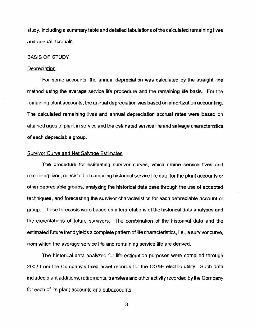
study, including a summary table and detailed tabulations of the calculated remaining lives
and annual accruals.
BASIS OF STUDY
Deweciation
For some accounts, the annual depreciation was calculated by the straight line
method using the average service life procedure and the remaining life basis. For the
remaining plant accounts, the annual depreciation was based on amortization accounting.
The calculated remaining lives and annual depreciation accrual rates were based on
attained ages of plant in service and the estimated service life and salvage characteristics
of each depreciable group.
Survivor Curve and Net Salvaae Estimates
The procedure for estimating survivor curves, which define service lives and
remaining lives, consisted of compiling historical service life data for the plant accounts or
other depreciable groups, analyzing the historical data base through the use of accepted
techniques, and forecasting the survivor characteristics for each depreciable account or
group. These forecasts were based on interpretations of the historical data analyses and
the expectations of future survivors. The combination of the historical data and the
estimated future trend yields a complete pattern of life characteristics, Le., a survivor curve,
from which the average service life and remaining service life are derived.
The historical data analyzed for life estimation purposes were compiled through
2002 from the Company’s fixed asset records for the OG&E electric utility. Such data
included plant additions, retirements, transfers and other activity recorded by the Company
for each of its plant accounts and subaccounts,
1-3
The estimates of net salvage by account incorporated a review of experienced costs
of removal and salvage related to plant retirements, and consideration of trends exhibited
by the historical data for the OG&E electric utility. Each component of net salvage, Le.,
cost of removal and salvage, was stated in dollars and as a percent of retirement.
An understanding of the function of the plant and information with respect to the
reasons for past retirements and the expected causes of future retirements was obtained
through discussions with operating and management personnel. The supplemental
information obtained in this manner was considered in the interpretation and extrapolation
of the statistical analyses.
Calculation of Depreciation
The depreciation accrual rates were calculated using the straight line method, the
remaining life basis and the average service life depreciation procedure. The continuation
of amortization accounting for certain accounts is recommended because of the
disproportionate plant accounting effort required when compared to the minimal original
cost of the large number of items in these accounts. An explanation of the calculation of
annual and accrued amortization is presented on page 11-28 of the report.
1-4

PART II. METHODS USED IN
THE ESTIMATION OF DEPRECIATION
11-1

PART 11. METHODS USED IN THE ESTIMATION OF DEPRECIATION
DEPRECIATION
Depreciation, as defined in the Uniform System of Accounts, is the loss in service
value not restored by current maintenance, incurred in connection with the consumption
or prospective retirement of electric and gas plant in the course of service from causes
which are known to be in current operation and against which the utility is not protected by
insurance. Among the causes to be given consideration are wear and tear, decay, action
of the elements, inadequacy, obsolescence, changes in the art, changes in demand,
requirements of public authorities, and, in the case of natural gas companies, the
exhaustion of natural resources.
Depreciation, as used in accounting, is a method of distributing fixed capital costs,
less net salvage, over a period of time by allocating annual amounts to expense. Each
annual amount of such depreciation expense is part of that year's total cost of providing
utility service. Normally, the period of time over which the fixed capital cost is allocated to
the cost of service is equal to the period of time over which an item renders service, that
is, the item's service life. The most prevalent method of allocation is to distribute an equal
amount of cost to each year of service life. This method is known as the straight line
method of depreciation.
The calculation of annual depreciation based on the straight line method requires
the estimation of average life and salvage. These subjects are discussed in the sections
which follow.
11-2
SERVICE LIFE AND NET SALVAGE ESTIMATION
Averase Service Life
The use of an average service life for a property group implies that the various units
in the group have different lives. Thus, the average life may be obtained by determining
the separate lives of each of the units, or by constructing a survivor curve by plotting the
number of units which survive at successive ages. A discussion of the general concept of
survivor curves is presented. Also, the Iowa type survivor curves are reviewed.
Survivor Curves
The survivor curve graphically depicts the amount of property existing at each age
throughout the life of an original group. From the survivor curve, the average life of the
group, the remaining life expectancy, the probable life, and the frequency curve can be
calculated. In Figure 1, a typical smooth survivor curve and the derived curves are
illustrated. The average life is obtained by calculating the area under the survivor curve,
from age zero to the maximum age, and dividing this area by the ordinate at age zero. The
remaining life expectancy at any age can be calculated by obtaining the area under the
curve, from the observation age to the maximum age, and dividing this area by the percent
surviving at the observation age. For example, in Figure 1 , the remaining life at age 30 is
equal to the crosshatched area under the survivor curve divided by 29.5 percent surviving
at age 30. The probable life at any age is developed by adding the age and remaining life.
If the probable life of the property is calculated for each year of age, the probable life curve
shown in the chart can be developed. The frequency curve presents the number of units
retired in each age interval and is derived by obtaining the differences between the amount
of property surviving at the beginning and at the end of each interval.
11-3

/
-H - Q) U 0
11-4
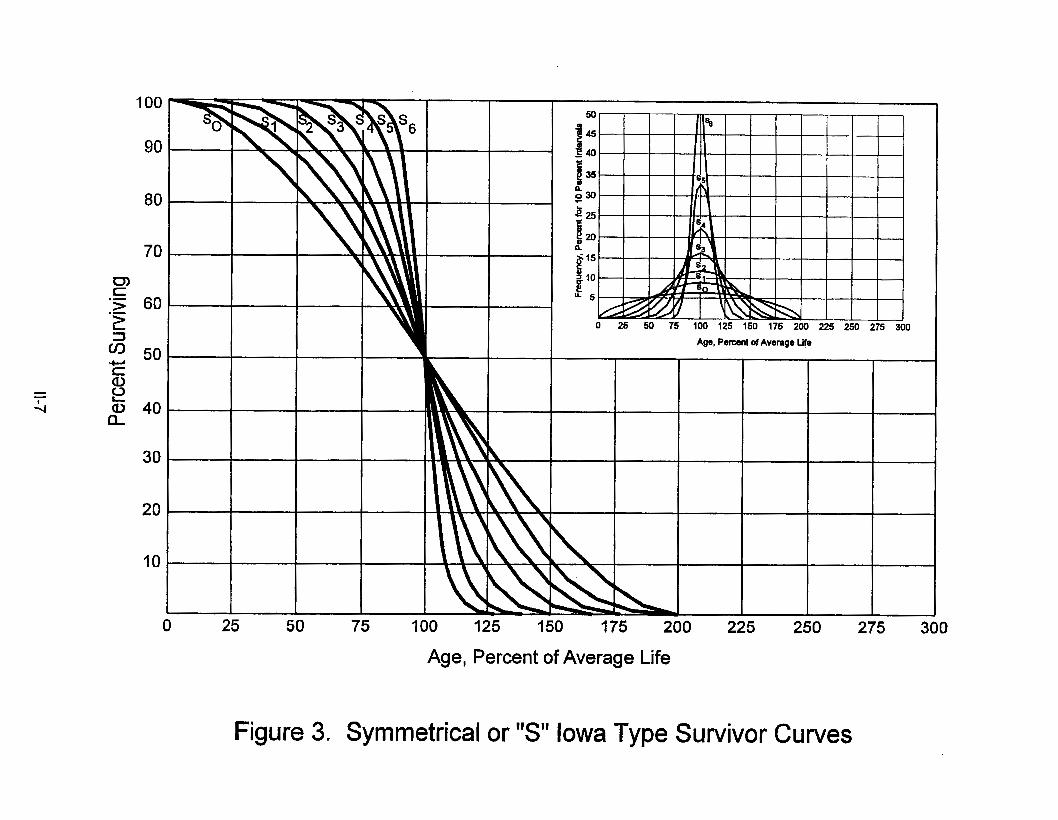
Iowa TvDe Curves. The range of survivor characteristics usually experienced by
utility and industrial properties is encompassed by a system of generalized survivor curves
known as the Iowa type curves. There are four families in the Iowa system, labeled in
accordance with the location of the modes of the retirements in relationship to the average
life and the relative height of the modes. The left moded or L curves, presented in Figure
2, are those in which the greatest frequency of retirement occurs to the left of, or prior to,
average service life. The symmetrical moded or S curves, presented in Figure 3, are those
in which the greatest frequency of retirement occurs at average service life. The right
moded or R curves, presented in Figure 4, are those in which the greatest frequency
occurs to the right of, or after, average service life. The origin moded or 0 curves,
presented in Figure 5, are those in which the greatest frequency of retirement occurs at the
origin, or immediately after age zero. The letter designation of each family of curves (L,
SI R or 0) represents the location of the mode of the associated frequency curve with
respect to the average service life. The numerical subscripts represent the relative heights
of the modes of the frequency curves within each family.
The Iowa curves were developed at the Iowa State College Engineering Experiment
Station through an extensive process of observation and classification of the ages at which
industrial property had been retired. A report of the study which resulted in the
classification of property survivor characteristics into 1 8 type curves, which constitute three
of the four families, was published in 1935 in the form of the Experiment Station's Bulletin
125.' These type curves have also been presented in subsequent Experiment Station
'Winfrey, Robley. Statistical Analvses of Industrial ProPertv Retirements. Iowa State College, Engineering Experiment Station, Bulletin 125. 1935.
11-5

100
90
80
70 CT) c -- -5 60 2
CO + 50
$ 40
30
3
c a,
a.
20
10
0 25 50 75 I00 125 150 175 200 225 250 275 300
Age, Percent of Average Life
Figure 2. Left Modal or "L" Iowa Type Survivor Curves
1 oc
9c
8C
7C ul c .- '5 60 L
50 3
r: a
Q
-c.r
40
30
20
I O
25 50 75 I00 125 150 175 200 225 250 275 300 0
Age, Percent of Average Life
Figure 3. Symmetrical or "S" Iowa Type Survivor Curves

0 CD
0 ln
LL
11-8

100
90
80
70
60
50
40
30
20
10
I I I I I I
0 Age, Percent of Average Life
Figure 5. Origin Modal or "0" Iowa Type Survivor Curves
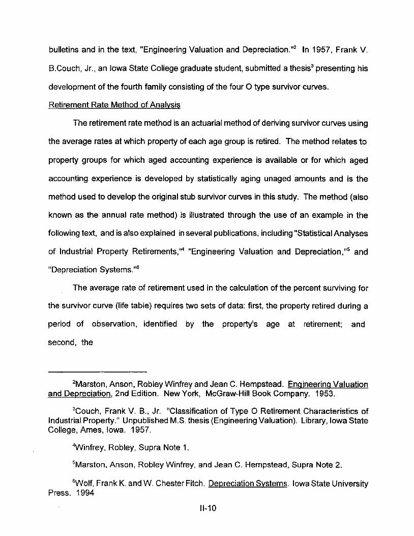
bulletins and in the text, "Engineering Valuation and Depreciation."' In 1957, Frank V
B.Couch, Jr., an Iowa State College graduate student, submitted a thesis3 presenting his
development of the fourth family consisting of the four 0 type survivor curves.
Retirement Rate Method of Analvsis
The retirement rate method is an actuarial method of deriving survivor curves using
the average rates at which property of each age group is retired. The method relates to
property groups for which aged accounting experience is available or for which aged
accounting experience is developed by statistically aging unaged amounts and is the
method used to develop the original stub survivor curves in this study. The method (also
known as the annual rate method) is illustrated through the use of an example in the
following text, and is also explained in several publications, including "Statistical Analyses
of Industrial Property retirement^,"^ "Engineering Valuation and Depreciati~n,"~ and
"Depreciation Systems."6
The average rate of retirement used in the calculation of the percent surviving for
the survivor curve (life table) requires two sets of data: first, the property retired during a
period of observation, identified by the property's age at retirement; and
second, the
'Marston, Anson, Robley Winfrey and Jean C. Hempstead. Enaineering Valuation and Depreciation, 2nd Edition. New York, McGraw-Hill Book Company. 1953.
3 C ~ ~ ~ h , Frank V. B., Jr. "Classification of Type 0 Retirement Characteristics of Industrial Property." Unpublished M.S. thesis (Engineering Valuation). Library, Iowa State College, Ames, Iowa. 1957.
4Winfrey, Robley, Supra Note 1.
'Marston, Anson, Robley Winfrey, and Jean C. Hempstead, Supra Note 2.
'Wolf, Frank K. and W. Chester Fitch. Depreciation Svstems. Iowa State University Press. 1994
11-10

property exposed to retirement at the beginnings of the age intervals during the same
period. The period of observation is referred to as the experience band, and the band of
years which represent the installation dates of the property exposed to retirement during
the experience band is referred to as the placement band. An example of the calculations
used in the development of a life table follows. The example includes schedules of annual
aged property transactions, a schedule of plant exposed to retirement, a life table and
illustrations of smoothing the stub survivor curve.
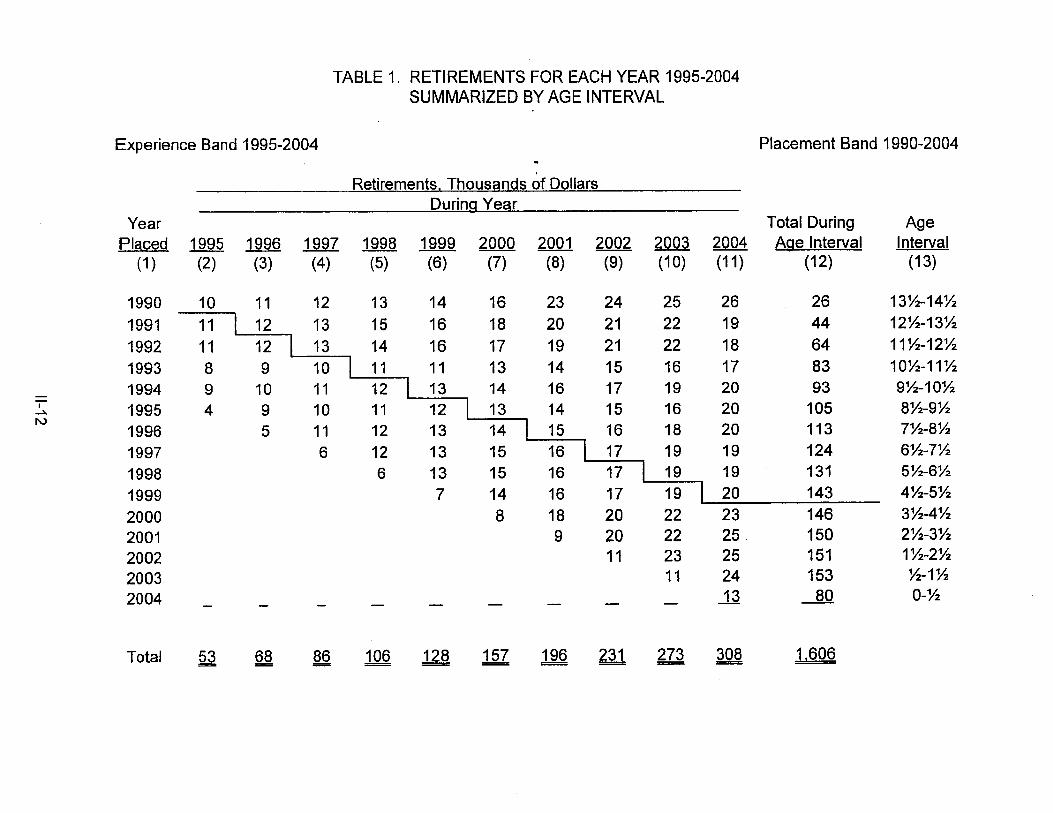
Schedules of Annual Transactions in Plant Records. The property group used to
illustrate the retirement rate method is observed for the experience band 1995-2004 during
which there were placements during the years 1990-2004. In order to illustrate the
summation of the aged data by age interval, the data were compiled in the manner
presented in Tables 1 and 2 on pages 11-12 and 11-13. In Table 1, the year of installation
(year placed) and the year of retirement are shown. The age interval during which a *<*+ ..-v&+- rl+. ' e -
retirement occurred is determined from this information. In the example which follows,
$10,000 of the dollars invested in 1990 were retired in 1995. The $10,000 retirement
occurred during the age interval between 4% and 5% years on the basis that approximately
one-half of the amount of property was installed prior to and subsequent to July 1 of each
year. That is, on the average, property installed during a year is placed in service at the
midpoint of the year for the purpose of the analysis. All retirements also are stated as
occurring at the midpoint of a one-year age interval of time, except the first age interval
which encompasses only one-half year.
The total retirements occurring in each age interval in a band are determined by
summing the amounts for each transaction year-installation year combination for that age
11-1 1
Experience Band 1995-2004
TABLE 1. RETIREMENTS FOR EACH YEAR 1995-2004 SUMMARIZED BY AGE INTERVAL
Placement Band 1990-2004 . Retirements, Thousands of Dollars
During Year Year Total During Age
(1 1 (2) (3) (4) (5) (6) (7) (8) (9) (10) (11) (12) (1 3) Placed 1995 1996 1997 1998 1999 2000 2001 2002 2003 2004 Age Interval Interval
1990 10 11 12 13 14 16 23 24 25 26 26 13%-14% 1991 7 12 13 15 16 18 20 21 22 19 44 12%-13% 1992 11 '71 ;i , 14 16 17 19 21 22 18 1993 8 11 11 13 14 15 16 17
64 11%-12% a3 10%-11%
1994 9 10 I 1 13 14 16 17 19 20 93 9%-I 0% 1995 4 9 10 11 121 13 14 15 16 20 105 8%-9% 1996 5 11 12 13 14 I 15 16 18 20 113 7%-8% 1997 1998 1999 2000 2001 2002 2003 2004 -
l6 I%-, ;: , :: ::: 6 12 13 15 6 13 15 16
7 14 16 17 20 143 8 18 20 22 23 146
9 20 22 25 150 11 23 25 151
11 24 153 - - 13 80 - - - - - -
1,606
6%-7?4 5%-6% 4%-5% 31/2-4% 21/2-3% 1 w-2% %-I % 0-%

TABLE 2. OTHER TRANSACTIONS FOR EACH YEAR 1995-2004 SUMMARIZED BY AGE INTERVAL
Experience Band 1995-2004
Acquisitions, Transfers. and Sales, Thousands of Dollars During Year
Year Placed 1995 1996 1997 1998 1999 2000 (1) (2) (3) (4) (5) (6) (7)
I990 - 1991 - 1992 - 1993 - 1994 -
- - 1995 --L 1996
1997 1998 I999 2000 2001 2002 2003 2004 -
I
0
- - - - - - = - - = = Total
" Transfer Affecting Exposures at Beginning of Year.
"Sale with Continued Use.
b Transfer Affecting Exposures at End of Year.
Parentheses denote Credit amount.
Placement Band 1990-2004
Total During Age Aae Interval Interval
(1 2) (1 3)
13%-14% 12%-I 3% 11%-121/2 l O % - I l % 9%-10% 8?4-91/2 7%-81/2 6%-7% 5%6% 4%-5% 3%-4% 2?4-3% 1 %-2% %-I % 0-%

interval. For example, the total of $143,000 retired for age interval 4%5% is the sum of
the retirements entered on Table 1 immediately above the stairstep line drawn on the table
beginning with the 1995 retirements of 1990 installations and ending with the 2004
retirements of the 1998 installations. Thus, the total amount of 143 for age interval 4%-5%
equals the sum of:
10 + 12 + 13 + 11 + 13 + 13 + 15 + 17 + 19 + 20.
In Table 2, other transactions which affect the group are recorded in a similar
manner. The entries illustrated include transfers and sales. The entries which are credits
to the plant account are shown in parentheses. The items recorded on this schedule are
not totaled with the retirements, but are used in developing the exposures at the beginning
of each age interval.
Schedule of Plant Exposed to Retirement. The development of the amount of plant
exposed to retirement at the beginning of each age interval is illustrated in Table 3 on page
11-15.
The surviving plant at the beginning of each year from 1995 through 2004 is
recorded by year in the portion of the table headed "Annual Survivors at the Beginning of
the Year." The last amount entered in each column is the amount of new plant added to
the group during the year. The amounts entered in Table 3 for each successive year
following the beginning balance or addition are obtained by adding or subtracting the net
entries shown on Tables 1 and 2. For the purpose of determining the plant exposed to
retirement, transfers-in are considered as being exposed to retirement in this group at the
beginning of the vear in which they occurred, and the sales and transfers-out are
considered to be removed from the plant exposed to retirement at the beqinninq of the
followina vear.
11-14

TABLE 3. PLANT EXPOSED TO RETIREMENT JANUARY 1 OF EACH YEAR 1995-2004 SUMMARIZED BY AGE INTERVAL
Experience Band 1995-2004 Placement Band 1990-2004
Exposures. Thousands of Dollars Annual Survivors at the Beainnina of the Year
Total at Beginning
Year of Age Age
(1) (2) (3) (4) (5) (6) (7) (8) (9) (1 0) (1 1) (12) (1 3) . Interval Placed 1995 1996 1997 1998 1999 2000 2001 2002 2003 2004 Interval
1990 255 245 234 222 209 195 239 216 192 167 167 131/2-14'!4 212 194 174 153 131 323 121/2-13%
1992 224 205 184 162 53 1 11M-12% 1993 330 300 289 276 262 242 226 823 10%111/2 Igg1 ?%!--] i! 1:: :i; 241
1994 376 367 357 346 1995 420" 41 6 407 397 1996 460" 455 444 1997 510" 504 1998 580a 1999 2000 200 1 2002 2003 2004
I 334 32 I 307 297 280 26 1 1,097 91/2-101/2 386 I 374 361 347 332 31 6 1,503 8%-9?4 432 419 I 405 390 374 356 1,952 7%-8% 492 479 464 I 448 43 1 412 2,463 6?4-7?4 574 56 1 546 530 I 501 482 3,057 5?4-6?4 660" 653 639 623 628 I 609 3,789 41/2-51/2
750" 742 724 685 663 4,332 31/2-41/2
960" 949 926 5,719 1 1/2-21/2 1,080" 1,069 6,579 %-I ?4
850a 841 82 1 799 4,955 21/2-31/2
1,220" 7.490 0-1/2
Total 1,975 2,382 2.824 3,318 3.872 4.494 - 5.247 6.017 - - 6.852 7,799 44,780
a Additions during the year.

Thus, the amounts of plant shown at the beginning of each year are the amounts of plant
from each placement year considered to be exposed to retirement at the beginning of each
successive transaction year. For example, the exposures for the installation year 1999 are
calculated in the following manner:
Exposures at age 0 = amount of addition = $750,000 Exposures at age W = $750,000 - $8,000 = $742,000 Exposures at age 1% = $742,000 - $18,000 = $724,000 Exposures at age 2% = $724,000 - $20,000 - $19,000 = $685,000 Exposures at age 3% = $685,000 - $22,000 = $663,000
For the entire experience band 1995-204, the total exposures at the beginning of
an age interval are obtained by summing diagonally in a manner similar to the summing
of the retirements during an age interval (Table 1). For example, the figure of 3,789,
shown as the total exposures at the beginning of age interval 4%5%, is obtained by
summing:
255+268+284+311 +334+374+405+448+501 +609.
Original Life Table. The original life table, illustrated in Table 4 on page 11-17, is
developed from the totals shown on the schedules of retirements and exposures, Tables
1 and 3, respectively. The exposures at the beginning of the age interval are obtained from
the corresponding age interval of the exposure schedule, and the retirements during the
age interval are obtained from the corresponding age interval of the retirement schedule.
The retirement ratio is the result of dividing the retirements during the age interval by the
exposures at the beginning of the age interval. The percent surviving at the beginning of
each age interval is derived from survivor ratios, each of which equals one
11-1 6

TABLE 4. ORIGINAL LIFE TABLE CALCULATED BY THE RETIREMENT RATE METHOD
Experience Band 1995-2004 Placement Band 1990-2004
(Exposure and Retirement Amounts are in Thousands of Dollars)
Age at Beginning of
Interval (1 1
0.0 0.5 1.5 2.5 3.5 4.5 5.5 6.5 7.5 8.5 9.5 10.5 11.5 12.5 13.5
Total
Exposures at Beginning of Acre Interval
(2)
7,490 6,579 5,719 4,955 4,332 3,789 3,057 2,463 1,952 1,503 1,097 823 53 1 323 167
44,780
Retirements During Age
Interval (3)
80 153 151 150 146 143 131 124 113 105 93 83 64 44 2
1,606
Retirement Ratio (4)
0.01 07 0.0233 0.0264 0.0303 0.0337 0.0377 0.0429 0.0503 0.0579 0.0699 0.0848 0.1009 0.1205 0.1 362 0.1557
Survivor Ratio (5)
0.9893 0.9767 0.9736 0.9697 0.9663 0.9623 0.9571 0.9497 0.9421 0.9301 0.9152 0.8991 0.8795 0.8638 0.8443
Percent Surviving at Beginning of Age Interval
(6)
100.00 98.93 96.62 94.07 91 -22 88.15 84.83 81.19 77.1 1 72.65 67.57 61.84 55.60 48.90 42.24 35.66
Column 2 from Table 3, Column 12, Plant Exposed to Retirement. Column 3 from Table 1, Column 12, Retirements for Each Year. Column 4 = Column 3 divided by Column 2. Column 5 = 1.0000 minus Column 4. Column 6 = Column 5 multiplied by Column 6 as of the Preceding Age Interval.
11-1 7

minus the retirement ratio. The percent surviving is developed by starting with 100% at
age zero and successively multiplying the percent surviving at the beginning of each
interval by the survivor ratio, i.e., one minus the retirement ratio for that age interval. The
calculations necessary to determine the percent surviving at age 5% are as follows:
88.15 Exposures at age 4% = 3,789,000 Retirements from age 4% to 5% = 143,000 Retirement Ratio = 143,000 +3,789,000 = 0.0377 Survivor Ratio - Percent surviving at age 5% = (88.15) x (0.9623) = 84.83
- - Percent surviving at age 4%
1.000 - 0.0377 = 0.9623 -
The totals of the exposures and retirements (columns 2 and 3) are shown for the
purpose of checking with the respective totals in Tables 1 and 3. The ratio of the total
retirements to the total exposures, other than for each age interval, is meaningless.
The original survivor curve is plotted from the original life table (column 6, Table 4).
When the curve terminates at a percent surviving greater than zero, it is called a stub
survivor curve. Survivor curves developed from retirement rate studies generally are stub
curves.
Srnoothina the Oriainal Survivor Curve. The smoothing of the original survivor curve
eliminates any irregularities and serves as the basis for the preliminary extrapolation to
zero percent surviving of the original stub curve. Even if the original survivor curve is
complete from 100% to zero percent, it is desirable to eliminate any irregularities, as there
is still an extrapolation for the vintages which have not yet lived to the age at which the
curve reaches zero percent. In this study, the smoothing of the original curve with estab-
lished type curves was used to eliminate irregularities in the original curve.
The Iowa type curves are used in this study to smooth those original stub curves
which are expressed as percents surviving at ages in years. Each original survivor curve
was compared to the Iowa curves using visual and mathematical matching in order to
11-18
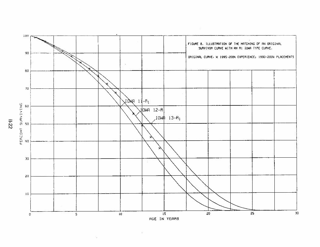
determine the better fitting smooth curves. In Figures 6, 7, and 8, the original curve
developed in Table 4 is compared with the L, SI and R Iowa type curves which most nearly
fit the original survivor curve. In Figure 6, the L1 curve with an average life between 12 and
1 3 years appears to be the best fit. In Figure 7, the SO type curve with a 12-year average
life appears to be the best fit and appears to be better than the L1 fitting. In Figure 8, the
R I type curve with a 12-year average life appears to be the best fit and appears to be
better than either the L l or the SO. In Figure 9, the three fittings, 12-L1, 12-SO and 12-R1
are drawn for comparison purposes. It is probable that the 12-R1 Iowa curve would be
selected as the most representative of the plotted survivor characteristics of the group,
assuming no contrary relevant factors external to the analysis of historical data.
Simulated Plant Balance Method
The Simulated plant balance method of life analysis is a statistical procedure by
which experienced average service life and survivor characteristics are inferred through a
series of approximations in which several average service life and survivor curve
combinations are tested. The testing procedure consists of applying survivor ratios defined
by the average service life and survivor curve combinations being tested to historical plant
additions and comparing the resulting calculated, or simulated, surviving balances with the
actual surviving balances.
11-1 9

I
I
0 0 - 0 0
m Q x 0 ru
11-20

1 oc
90
a0
70
I
> I
2 I- Z w U K w 40 a
30
20
10
0 5 10 15 RGE IN YERRS
20 25 30
100
90
80
70
U z 60 e
> > 3 m 50
z W U U
L
- - a
- k -
-
w 40
30
20
IO
RGE I N YEARS

l o o F
:T 10 0
FIGURE 9. ILLUSTRRTION OF THE MATCHING OF RN ORIGINAL SURVIVOR CURVE WITH L I , 50 AND R I IOWA TYPE CURVES.
ORIGINAL CURVE: X 1995-200'4 EXPERIENCE: 1990-200'4 PLACEMENTS
20 25 30
RGE IN YERRS
Each year-end book balance is the sum of the plant surviving from the original
annual additions. Each calculated year-end balance is the sum of the simulated plant
surviving from the same original annual additions. The simulated survivors are calculated
for each vintage by multiplying the original additions by the percent surviving corresponding
to the age of the vintage as of the date of the yearend balances being simulated. This
procedure is repeated until a series of simulated balances is calculated. The balances are
then compared with the book balances to determine which average service life and survivor
curve combinations result in calculated balances most nearly simulating the progression
of actual balances.
The simulated plant balance method is presented in greater detail in the Edison
Electric Institute’s publication, “Methods of Estimating Utility Plant Life’’.7
Service Life Considerations
The service life estimates were based on judgment which considered a number of
factors. The primary factors were the current Company policies and outlook as determined
during conversations with management and the survivor curve estimates from previous
studies of both the holding company and the electric utility assets as well as other utility
companies.
For the 10 plant accounts and subaccounts for which survivor curves were
estimated, the statistical analyses using the retirement rate or simulated plant record
methods did not provide specific indicators of survivor patterns. Therefore, judgment
incorporating the estimates of other utilities was a major factor in determining service life.
‘A Report of the Engineering Subcommittee of the Depreciation Accounting Committee, Edison Electric Institute. Publication No. 51 -23. Published 1952.
11-24
These accounts represent 8 percent of depreciable plant. The estimates of the remaining
accounts were based on amortization periods.
Salvaqe Analvsis
The estimates of net salvage by account were based in part on historical data
compiled through 2002 for the OG&E electric utility. Cost of removal and salvage were
expressed as percents of the original cost of plant retired, both on annual and three-year
moving average bases. The most recent five-year average also was calculated for
consideration. The net salvage estimates by account are expressed as a percent of the
original cost of plant retired.
Net Salvaqe Considerations
The estimates of future net salvage are expressed as percentages of surviving plant
in service, i.e., all future retirements. In cases in which removal costs are expected to
exceed salvage receipts, a negative net salvage percentage is estimated. The net salvage
estimates were based on judgment which incorporated analyses of historical cost of
removal and salvage data, expectations with respect to future removal requirements and
markets for retired transportation and power operated equipment.
Statistical analyses for the transportation equipment subaccount and power
operated equipment account of the OG&E electric utility were utilized in determining a
reasonable net salvage percent. All other accounts were amortized, therefore, a zero
percent for net salvage was recommended.
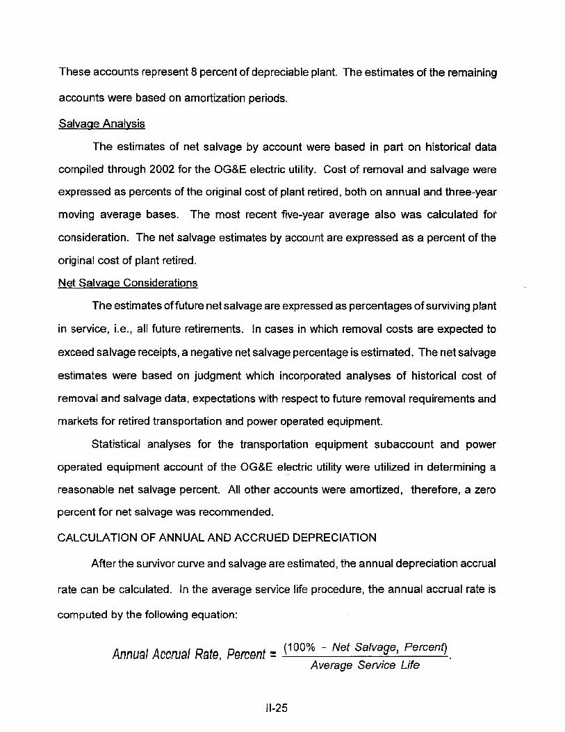
CALCULATION OF ANNUAL AND ACCRUED DEPRECIATION
After the survivor curve and salvage are estimated, the annual depreciation accrual
rate can be calculated. In the average service life procedure, the annual accrual rate is
computed by the following equation:
(100% - Net Salvage, Percenf) Average Sewice Life
Annual Accrual Rate, Percent =
11-25
The calculated accrued depreciation for each depreciable property group represents that
portion of the depreciable cost of the group which will not be allocated to expense through
future depreciation accruals if current forecasts of life characteristics are used as a basis
for straight line depreciation accounting.
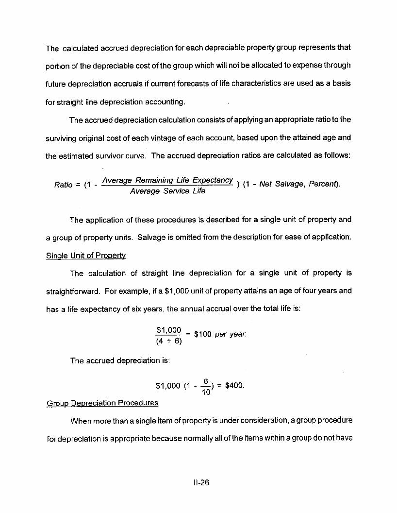
The accrued depreciation calculation consists of applying an appropriate ratio to the
surviving original cost of each vintage of each account, based upon the attained age and
the estimated survivor curve. The accrued depreciation ratios are calculated as follows:
Average Remaining Life Expectancy Average Service Life
- Net Salvage, Pen=enf). Ratio = (1 -
The application of these procedures is described for a single unit of property and
a group of property units. Salvage is omitted from the description for ease of application.
Sinale Unit of ProDertv
The calculation of straight line depreciation for a single unit of property is
straightforward. For example, if a $1,000 unit of property attains an age of four years and
has a life expectancy of six years, the annual accrual over the total life is:
$'*Oo0 = $100 per year. (4 + 6)
The accrued depreciation is:
6 10
$1,000 (1 - -) = $400.
Group Depreciation Procedures
When more than a single item of property is under consideration, a group procedure
for depreciation is appropriate because normally all of the items within a group do not have
11-26

identical service lives, but have lives that are dispersed over a range of time. There are
two primary group procedures, namely, average service life and equal life group.
Remainina Life Annual Accruals. For the purpose of calculating remaining life
accruals as of December 31, 2004, the depreciation reserve for each plant account is
allocated among vintages in proportion to the calculated accrued depreciation for the
account. Explanations of remaining life accruals and calculated accrued depreciation
follow. The detailed calculations as of December 31, 2004, are set forth in the Results of
Study section of the report.
Averaae Service Life Procedure. In the average service life procedure, the
remaining life annual accrual for each vintage is determined by dividing future book
accruals (original cost less book reserve) by the average remaining life of the vintage. The
average remaining life is a directly weighted average derived from the estimated future
survivor curve in accordance with the average service life procedure.
The calculated accrued depreciation for each depreciable property group represents
that portion of the depreciable cost of the group which would not be allocated to expense
through future depreciation accruals, if current forecasts of life characteristics are used as
the basis for such accruals. The accrued depreciation calculation consists of applying an
appropriate ratio to the surviving original cost of each vintage of each account, based upon
the attained age and service life. The straight line accrued depreciation ratios are
calculated as follows for the average service life procedure:
Average Remaining Life Average Service Life ’
Ratio =
11-27
CALCULATION OF ANNUAL AND ACCRUED AMORTIZATION
Amortization, as defined in the Uniform System of Accounts, is the gradual
extinguishment of an amount in an account by distributing such amount over a fixed period,
over the life of the asset or liability to which it applies, or over the period during which it is
anticipated the benefit will be realized. Normally, the distribution of the amount is in equal
amounts to each year of the amortization period.
The calculation of annual and accrued amortization requires the selection of an
amortization period. The amortization periods used in this report were based on judgment
which incorporated a consideration of the period during which the assets will render most
of their service, the amortization periods and service lives used by other utilities, and the
service life estimates previously used for the asset under depreciation accounting.
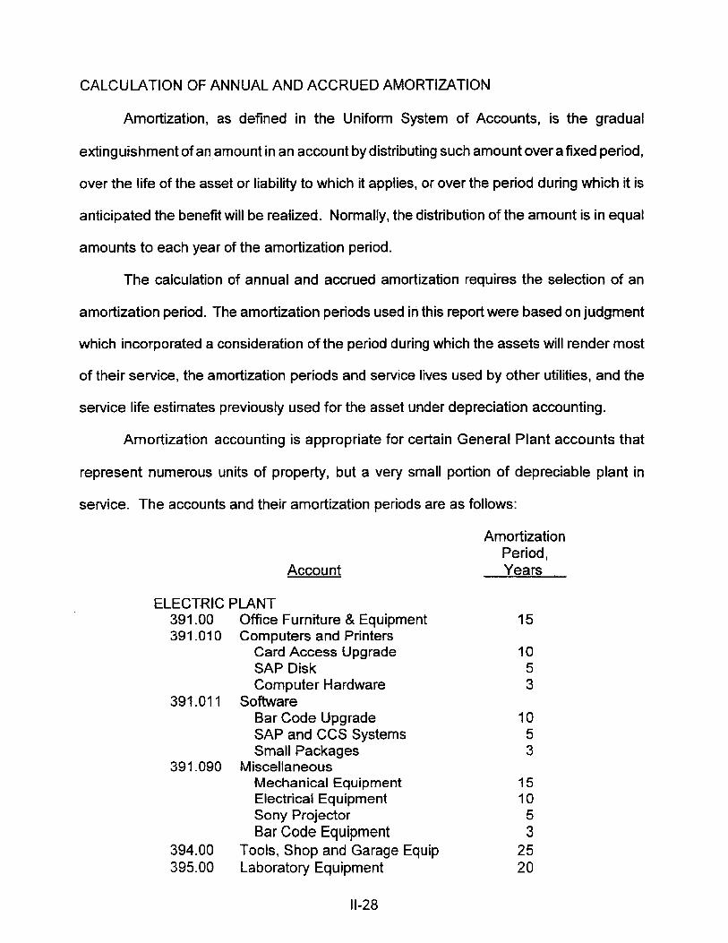
Amortization accounting is appropriate for certain General Plant accounts that
represent numerous units of property, but a very small portion of depreciable plant in
service. The accounts and their amortization periods are as follows:
Account
ELECTRIC PLANT 391 .OO 391.01 0 Computers and Printers
Card Access Upgrade SAP Disk Computer Hardware
Bar Code Upgrade SAP and CCS Systems Small Packages
Mechanical Equipment Electrical Equipment Sony Projector Bar Code Equipment
Office Furniture & Equipment
391.01 1 Software
391.090 Miscellaneous
394.00 395.00 Laboratory Equipment
Tools, Shop and Garage Equip
Amortization Period, Years
15
10 5 3
10 5 3
15 10 5 3
25 20
11-28

Account
Amortization Period , Years
397.00 Communication Equipment Radio Service 15 PBX System 10 Voice Mail System 8 Radio Equipment 5
398.00 Miscellaneous Equipment 15
For the purpose of calculating annual amortization amounts as of December 31,
2004, the book or ratemaking book depreciation reserve for each plant account or
subaccount is assigned or allocated to vintages. The reserve assigned to vintages with an
age greater than the amortization period is equal to the vintage’s original cost. The
remaining reserve is allocated among vintages with an age less than the amortization
period in proportion to the calculated accrued amortization. The calculated accrued
amortization is equal to the original cost multiplied by the ratio of the vintage’s age to its
amortization period. The annual amortization amount is determined by dividing the future
amortizations (original cost less allocated book reserve) by the remaining period of
amortization for the vintage.
11-29

PART 111. RESULTS OF STUDY
Ill-I
PART 111. RESULTS OF STUDY
QUALIFICATION OF RESULTS
The calculated annual depreciation accrual rates are the principal results of the
study. Continued surveillance and periodic revisions are normally required to maintain
continued use of appropriate annual depreciation accrual rates. An assumption that
accrual rates can remain unchanged over a long period of time implies a disregard for the
inherent variability in service lives and salvage and for the change of the composition of
property in service. The annual accrual rates were calculated in accordance with the
straight line remaining life method of depreciation using the annual service life procedure
based on estimates which reflect considerations of current historical evidence and
expected future conditions.
The annual depreciation accrual rates are applicable specifically to the general plant
in service as of December 31, 2004. For most plant accounts, the application of such
rates to future balances that reflect additions subsequent to December 31, 2004, is
reasonable for a period of three to five years.
DESCRIPTION OF DEPRECIATION TABULATIONS
A summary of the results of the study, as applied to the original cost of general
plant at December 31,2004, is presented on page 111-4 of this report. The schedule sets
forth the original cost, the book reserve, future accruals, the calculated annual depreciation
rate and amount, and the corhposite remaining life related to general plant.
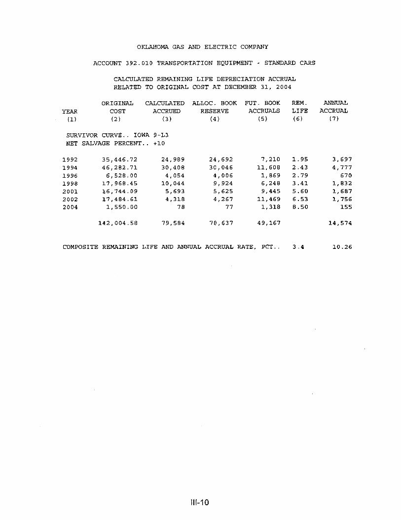
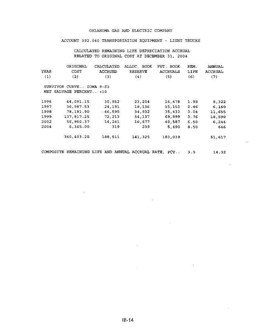
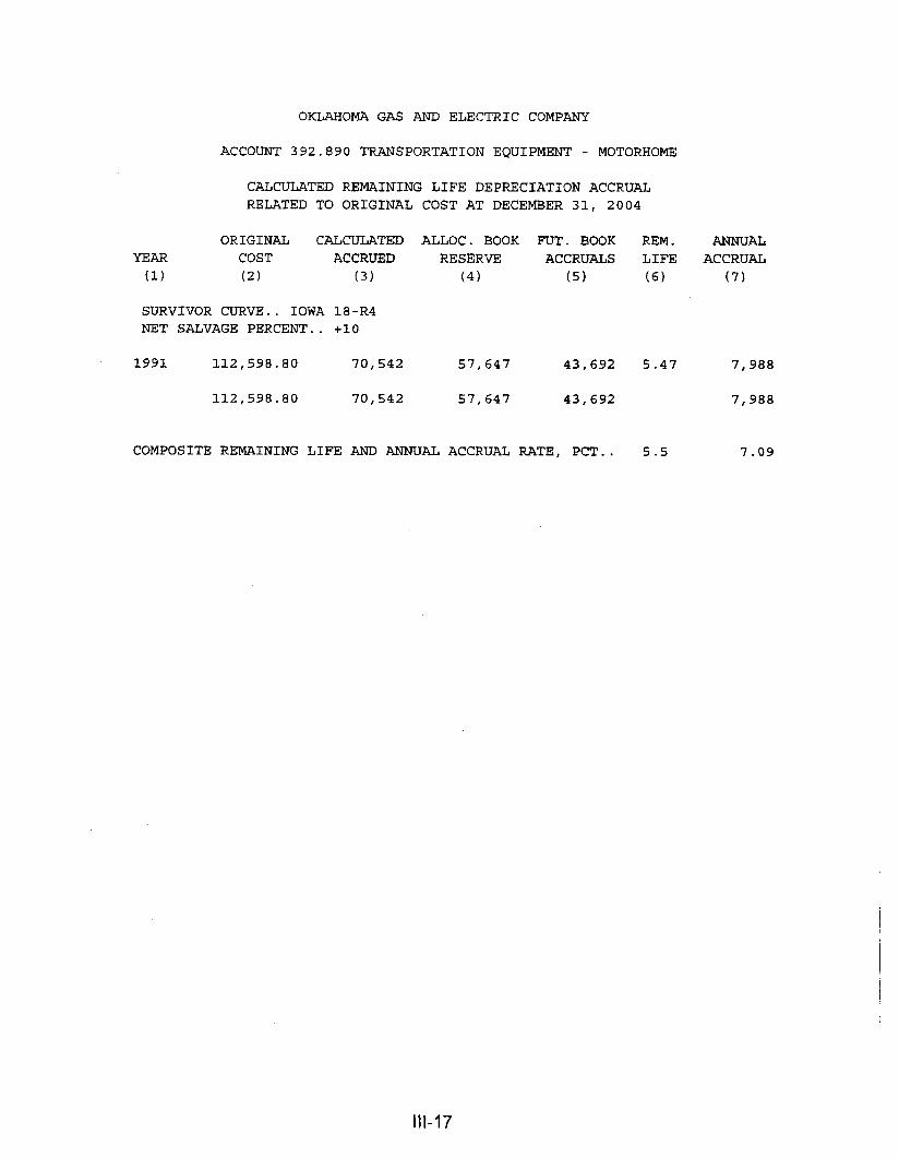
The tables of the calculated annual depreciation accruals are presented in account
sequence in the section titled "Depreciation Calculations." The tables indicate the
estimated survivor curve and salvage percent for the account and set forth, for each
111-2

installation year, the original cost, the calculated accrued depreciation, the allocated book
reserve, future accruals, the remaining life and the calculated annual accrual amount.
111-3
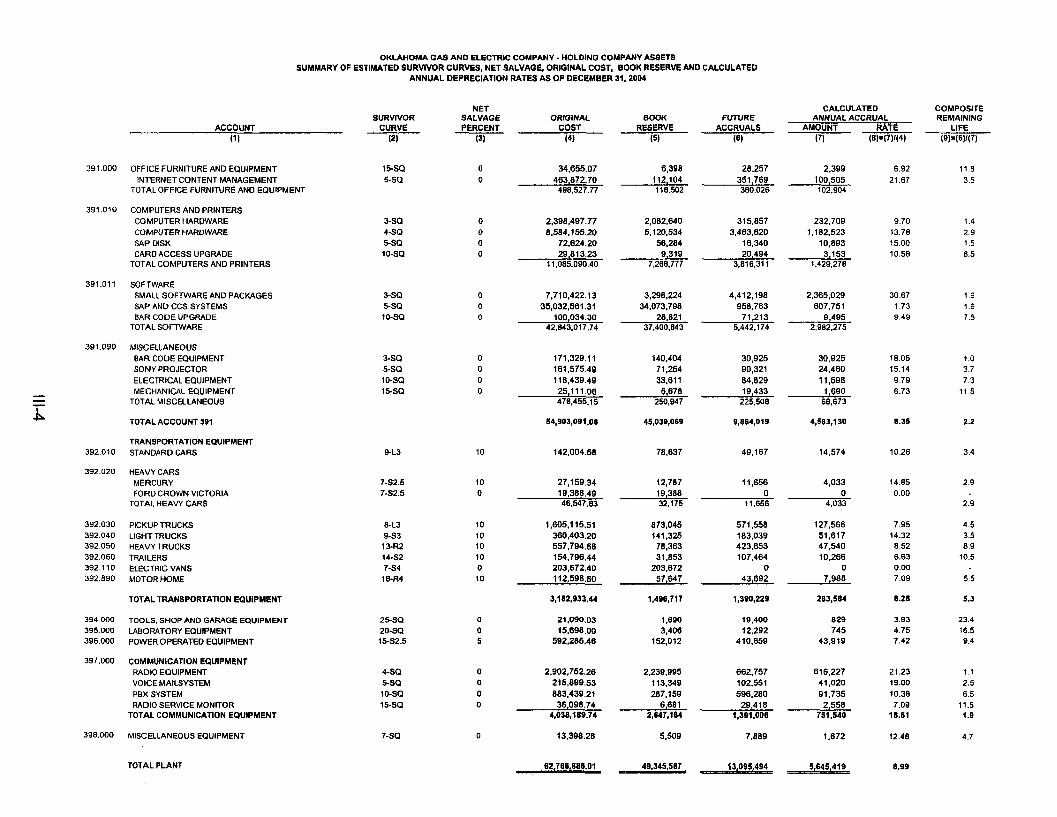
OKLAHOMA GAS AND ELECTRIC COMPANY -HOLDING COMPANY ASSETS SUMMARY OF ESTIMATED SURVIVOR CURVES, NET SALVAGE, ORIGINAL COST, BOOK RESERVE AND CALCULATED
ANNUAL DEPREClATlON RATES AS OF DECEMBER 31,2004
CALCULATED COMPOSITE REMAINING
LIFE (9)=(6)47)
NET SALVAGE PERCENT
(3)
0 0
0 0 0 0
0 0 0
0 0 0 0
10
10 0
10 10 10 10 0 10
0 0 5
0 0 0 0
0
ORIGINAL SURVIVOR CURVE
(2)
6OOK FUTURE ANNUAL ACCRUAL RESERVE ACCRUALS AMOUNT RATE
(5) (6) (7) (8)=(7)1(4) ACCOUNT
(1)
OFFICE FURNITURE AND EQUIPMENT INTERNET CONTENT MANAGEMENT
TOTAL OFFICE FURNITURE AND EQUIPMENT
COMPUTERS AND PRINTERS COMPUTER HARDWARE COMPUTER HARDWARE SAP DISK CAR0 ACCESS UPGRADE
TOTAL COMPUTERS AND PRINTERS
SOFTWARE SMALL SOFTWARE AND PACKAGES SAP AND CCS SYSTEMS BAR CODE UPGRADE
TOTAL SOFTWARE
MISCELLANEOUS BAR CODE EQUIPMENT SONY PROJECTOR ELECTRICAL EQUIPMENT MECHANICAL EQUIPMENT
TOTAL MISCELLANEOUS
TOTAL ACCOUNT 391
TRANSPORTATION EQUIPMENT STANDARD CARS
HEAVY CARS MERCURY FORD CROWN VICTORIA
TOTAL HEAVY CARS
PICKUP TRUCKS LIGHT TRUCKS HEAVY TRUCKS TRAILERS ELECTRIC VANS MOTOR HOME
TOTAL TRANSPORTATION EQUIPMENT
TOOLS, SHOP AND GARAGE EQUIPMENT LABORATORY EQUIPMENT POWER OPERATED EQUIPMENT
COMMUNICATION EQUIPMENT RADIO EQUIPMENT VOICE MAILSYSTEM PBX SYSTEM RADIO SERVICE MONITOR
TOTAL COMMUNICATION EQUIPMENT
MISCELLANEOUS EQUIPMENT
COST (4)
391.000
391.010
391.011
391.090
392.010
392.020
392.030 392.040 392.050 392.060 392.110 392.890
394.000
395.000 396.000
397.000
398.000
15-SQ 5-SQ
6.92 21.67
9.70 13.78 15.00 10.58
30.67 1.73 9.49
18.05 15.14 9.79 6.73
8.35
10.26
14.85 0.00
7.95 14.32 8.52 6.63 0.00 7.09
8.28
3.93 4.75 7.42
21.23 19.00 10.38 7.09
18.61
12.48
8.99
11.8 3.5
34.655.07 463,872.70 498.527.77
6.398 112,104 118,502
28.257 351,769 380.026
2.399 100,505 102.904
3-SQ 4SQ 5-SQ lO-SQ
1.4 2.9 1.5 6.5
2.398,497.77 8.584.155.20
72.624.20 29,813.23
11.085.090.40
2,082.640 5,120,534
56.284 9,319
7.268.777
315,857 3,463,620
16,340 20,494
3.816.31 1
232,709 1.182.523
10.893 3.153
1.429.278
3-SQ 5-SQ 10-SQ
7,710.422.1 3 35,032,561 3 1
3,298,224 34.073.798
4.412.198 958.763
1.9 1.6 7.5
2,365,029 607,751
9,495 2,982.275
28,821 37.400.843
100,034.30 42,843,017.74
71.213 5,442,174
3-SQ 5-SQ 1 0-SQ 15-SQ
171.329,ll 161.575.49 118,439.49
1 .o 3.7 7.3
11.5
140,404 71,254 33.61 1 5.678
250,947
45,039,069
30,925 90,321 84.829 19,433 225.508
9,864,019
30.925 24.460 11,598 1,690
68,673
4.583.130
25.111.06 476,455.1 5
54,903,091.06 2.2
9-L3 142,004.58 78.637 49.167 14.574 3.4
27,159.34 742.5 7-S2.5
2.9
2.9
4.5 3.5 8.9
10.5
5.5
5.3
12.707 19,388 32,175
11,656 0
1 1,656
571 -558 183,039 423,653 107,464
0 43,692
1,390.229
19,400 12,292
410.659
4,033 0
4.033 19,388.49 46.547.83
8-L3 9 4 3 13-R2 1442 7-54 18-R4
1.605.1 15.51 360.403.20 557,794.68 154.796,44 203.672.40 112,598.80
3.182.933.44
21.090,03 15.698.00
592,285.46
127.566 51,617 47.540 10.266
0 7.988
263.584
829 745
43.919
873.045 141.325 78.363 31.853
203.672 57,647
1,496,711
1.890 3.406
152,012
25SQ 20-SQ 1542.5
23.4 16.5 9.4
4-SQ 5-SQ 10-SQ 15-SQ
1.1 2.5 6.5
11.5 1.9
4.7
2,902.752.26
883.439,21 36.098.74
4,038,189.74
13.398.28
215,899.53 616,227 41,020 91.735 2,558
751,540
1,672
2.239.995 113,349 287.159
6,681 2,647,184
5.509
662.757 102,551 596.280 29,418
1,391,006
7.889 7-SQ
TOTAL PLANT 62,786,686.01 49,345,587 5,645,419

DE PREC IATlON CALCULATIONS
111-5
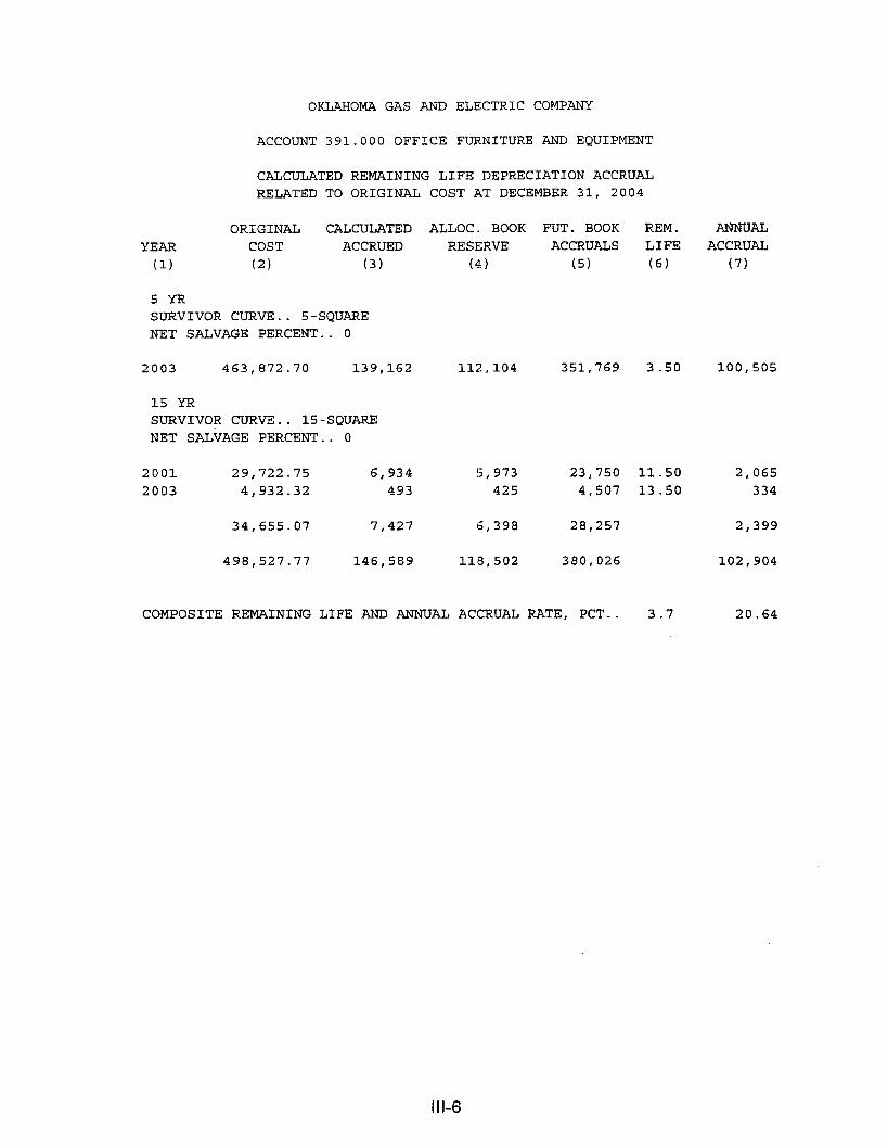
OKLAHOMA GAS AND ELECTRIC COMPANY
ACCOUNT 391.000 OFFICE FURNITURE AND EQUIPMENT
CALCULATED REMAINING LIFE DEPRECIATION ACCRUAL RELATED TO ORIGINAL COST AT DECEMBER 31, 2004
ORIGINAL CALCULATED YEAR COST ACCRUED (1) (2) (3)
5 Y R SURVIVOR CURVE.. 5-SQUARE NET SALVAGE PERCENT.. 0
2003 463,872.70 139,162
15 YR
NET SALVAGE PERCENT.. 0 SURVIVOR CURVE.. 15-SQUARE
2001 29,722.75 6,934 2003 4 , 932.32 493
34,655.07 7,427
498,527.77 146 , 589
ALLOC. BOOK RESERVE
( 4 )
112,104
5,973 425
6,398
118 , 502
FWT. BOOK ACCRUALS
(5)
351,769
23 , 750 4,507
28,257
380,026
REM. LIFE ( 6 )
3 .SO
11.50 13.50
COMPOSITE REMAINING LIFE AND ANNUAL ACCRUAL RATE, PCT.. 3.7
ANNUAL ACCRUAL
(7)
100,505
2,065 334
2,399
102 , 904
20.64
111-6

OKLAHOMA GAS AND ELECTRIC COMPANY
ACCOUNT 391.010 OFFICE FURNITURE AND EQUIPMENT-COMP&PRINTER
CALCULATED REMAINING LIFE DEPRECIATION ACCRUAL RELATED TO ORIGINAL COST AT DECEMBER 31, 2004
ORIGINAL CALCULATED YEAR COST ACCRUED (1) (2) (3)
COMPUTER HARDWARE SURVIVOR CURVE.. 3-SQUARE NET SALVAGE PERCENT.. 0
2001 1,820,860.12 1,820,860 2002 192,069.16 160 , 051 2003 377,071.03 188,536 2004 8,497.46 1,417
2,398,497.77 2,170,864
4 Y R SURVIVOR CURVE.. 4-SQUARE NET SALVAGE PERCENT.. 0
2001 2,030,668.20 1,776,835 2002 1,549,757.32 968,598 2003 2,344,064.39 879,024 2004 2,659,665.29 332,458
8,584,155.20 3,956,915
SAP DISK SURVIVOR CURVE.. 5-SQUARE NET SALVAGE PERCENT.. 0
2001 72,624.20 50,837
CARD ACCESS UPGRADE SURVIVOR CURVE.. 10-SQUARE NET SALVAGE PERCENT.. 0
2001 29,813.23 10,435
11,085,090.40 6,189,051
ALLOC. BOOK RESERVE
( 4 )
1,820,860 119,708 141,012
1,060
2,082,640
2 , 030,668 1,372,811 1 , 245,856
471,199
5,120 , 534
E'UT. BOOK ACCRUALS
(5)
72,361 236,059
7,437
315 , 857
176,946 1,098,208 2,188,466
3 , 463 , 620
REM. LIFE (6)
0.50 1.50 2.50
1.50 2.50 3.50
ANNUAL ACCRUAL
(7)
72 , 361 157,373
2,975
232 , 709
117,964 439,283 625 , 276
1,182 , 523
56,284 16,340 1-50 10,893
9,319
7,268,777
20,494
3,816,311
6.50 3,153
1,429,278
COMPOSITE REMAINING LIFE AND ANNUAL ACCRUAL RATE, PCT.. 2.7 12.89
111-7
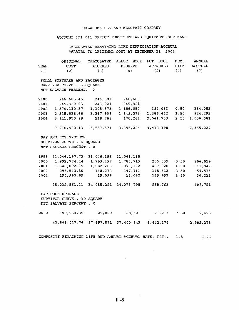
OKLAHOMA GAS AND ELECTRIC COMPANY
ACCOUNT 391.011 OFFICE FURNITURE AND EQUIPMENT-SOFTWARE
CALCULATED REMAINING LIFE DEPRECIATION ACCRUAL RELATED TO ORIGINAL COST AT DECEMBER 31, 2004
ORIGINAL CALCULATED ALLOC. BOOK FUT. BOOK YEAR COST ACCRUED RESERVE ACCRUALS (1) (2) (3) ( 4 ) (5)
SMALL SOFTWARE AND PACKAGES SURVIVOR CURVE.. 3-SQUARE NET SALVAGE PERCENT.. 0
2000 246,603.46 246 , 603 246 , 603 2 001 245,920.63 245 , 921 245 , 921 2002 1,570,110.37 1,308,373 1,186,057 384 , 053 2003 2,535,816.68 1,267,908 1,149,375 1,386,442 2004 3,111,970.99 518,766 470,268 2,641,703
7,710,422.13 3,587,571 3,298,224 4,412,198
SA?? AND CCS SYSTEMS SURVIVOR CURVE.. 5-SQUARE NET SALVAGE PERCENT.. 0
1998 31,046,157.73 31,046,158 31,046,158 2000 1,992,774.14 1,793,497 1,786,715 206,059 2001 1,546,092.19 1,082,265 1,078,172 467,920 2002 296,543.30 148 , 272 147,711 148,832 2004 150,993.95 15,099 15,042 135 , 952
35,032,561 -31 34,085,291 34,073,798 958 , 763
BAR CODE UPGRADE SURVIVOR CURVE.. 10-SQUARE NET SALVAGE PERCENT.. 0
2002 100,034.30 25,009 28,821 71,213
42,843,017.74 37,697,871 37,400,843 5,442,174
COMPOSITE REMAINING LIFE AND ANNUAL ACCRUAL RATE, PCT..
REM. ANNUAL LIFE ACCRUAL (6) (7)
0.50 384 , 053 1.50 924,295 2.50 1,056,681
2,365,029
0.50 206,059 1.50 311,947 2.50 59,533 4.50 30 , 212
607,751
7.50 9,495
2 , 982,275
1.8 6.96
111-8

OKLAHOMA GAS AND ELECTRIC COMPANY
ACCOUNT 391.090 OFFICE FURNITURE AND EQUIPMENT-MISC.
CALCULATED REMAINING LIFE DEPRECIATION ACCRUAL RELATED TO ORIGINAL COST AT DECEMBER 31, 2004
ORIGINAL CALCULATED YEAR COST ACCRUED (1) (2) ( 3 )
BAR CODE EQUIPMENT
NET SALVAGE PERCENT.. 0 SURVIVOR CURVE.. 3-SQUARE
2002 171,329.11 142,769
SONY PROJECTOR
NET SALVAGE PERCENT.. 0 SURVIVOR CURVE.. 5-SQUARE
2002 18,309.32 9,155 2003 109,698.90 32 , 910 2004 33,567.27 3,357
161,575.49 45,422
ELECTRICAL EQUIPMENT SURVIVOR CURVE.. 10-SQUARE NET SALVAGE PERCENT.. 0
2001 31,175.61 10 , 911 2002 82,910.66 20,728 2004 4,353 -22 218
118,439.49 31 , 857
MECHANICAL EQUIPMENT SURVIVOR CURVE.. 15-SQUARE NET SALVAGE PERCENT.. 0
2001 25,111.06 5,858
476,455.15 225,906
ALLOC. BOOK RESERVE
(4)
140,404
14,362 5.1, 626 5,266
71,254
11 , 512 21,869
230
33 , 611
5,678
250,947
FUT. BOOK ACCRUALS
(5)
30,925
3 , 947 58 , 073 28,301
90,321
19 , 664 61,042 4,123
84,829
19,433
225,500
REM. LIFE (6)
0.50
2.50 3.50 4.50
6.50 7.50 9.50
11 - 5 0
COMPOSITE REMAINING LIFE AND ANNUAL ACCRUAL RATE, PCT.. 3.3
ANNUAL ACCRUAL
(7)
30,925
1,579 16,592 6,289
24 , 460
3,025 8,139 434
11,598
1,690
60,673
14.41
111-9
OKLAHOMA GAS AND ELECTRIC COMPANY
ACCOUNT 392.010 TRANSPORTATION EQUIPMENT - STANDARD CARS
CALCULATED REMAINING LIFE DEPRECIATION ACCRUAL RELATED TO ORIGINAL COST AT DECEMBER 31, 2004
ORIGINAL CALCULATED ALLOC. BOOK FUT. BOOK REM. ANNLTAL YEAR COST ACCRUED RESERVE ACCRUALS LIFE ACCRUAL (1) (2) (3) (4) (5) ( 6 ) (7)
SURVIVOR CURVE.. IOWA 9-L3 NET SALVAGE PERCENT.. +10
1992 35,446.72 24,989 24,692 7,210 1.95 3,697 1994 46 , 282.71 30 , 408 30,046 11,608 2.43 4 , 777 1996 6,528.00 4,054 4,006 1,869 2.79 670 1998 17,968.45 10,044 9,924 6,248 3.41 1,832 2001 16,744.09 5,693 5,625 9,445 5.60 1,687 2002 17,484.61 4,318 4,267 11,469 6.53 1,756 2004 1,550.00 78 77 1,318 8.50 155
142,004.58 79,584 78,637 49,167 14 , 574
COMPOSITE REMAINING LIFE AND ANNUAL ACCRUAL RATE, PCT. . 3.4 10 -26
111-1 0

OKLAHOMA GAS AND ELECTRIC COMPANY
ACCOUNT 392.110 TRANSPORTATION EQUIPMENT - ELECTRIC VANS
CALCULATED REMAINING LIFE DEPRECIATION ACCRUAL RELATED TO ORIGINAL COST AT DECEMBER 31, 2004
ORIGINAL CALCULATED ALLOC. BOOK FWT. BOOK REM. m A L YEAR COST ACCRUED RESERVE ACCRUALS LIFE ACCRUAL (1) (2 1 (3) (4 1 (5) (6) (7)
SURVIVOR CURVE.. IOWA 7-S4 NET SALVAGE PERCENT.. 0
88,105.48 86,220 88 , 105 1993 1994 68,400.00 65 , 958 68,400 1995 47,166.92 44 , 606 47,167
203,672.40 196 , 784 203,672
COMPOSITE REMAINING LIFE AND ANNUAL ACCRUAL RATE, PCT.. 0.0 0.00
111-1 1

OKLAHOMA GAS AND ELECTRIC COMPANY
ACCOUNT 392.020 TFLANSPORTATION EQUIPMENT - HEAVY CARS
CALCULATED REMAINING LIFE DEPRECIATION ACCRUAL RELATED TO ORIGINAL COST AT DECEMBER 31, 2004
ORIGINAL CALCULATED ALLOC. BOOK FUT. BOOK REM. ANNUAL YEAR COST ACCRUED RESERVE ACCRUALS LIFE ACCRUAL (1) (2) (3 1 (4) (5) (6) (7)
MERCURY
NET SALVAGE PERCENT.. +10 SURVIVOR CURVE.. IOWA 7-S2.5
2000 27,159.34 14,351 12,787 11,656 2.89 4,033
FORD CROWN VICTORIA SURVIVOR CURVE.. IOWA 7-S2.5 NET SALVAGE PERCENT.. 0
1998 19,388 -49 14 , 458 19,388
46,547.83 28,809 32,175 11,656 4,033
COMPOSITE REMAINING LIFE AND ANNUAL ACCRUAL RATE, PCT.. 2.9 8.66
111-12

OKLAHOMA GAS AND ELECTRIC COMPANY
ACCOUNT 392.030 TRANSPORTATION EQUIPMENT - PICKUP TRUCKS
CALCULATED REMAINING LIFE DEPRECIATION ACCRUAL RELATED TO ORIGINAL COST AT DECEMBER 31, 2004
ORIGINAL CALCULATED ALLOC. BOOK F'UT. BOOK YEAR COST ACCRUED RESERVE ACCRUALS (1) (2) (3) (4) (5)
SURVIVOR CURVE.. IOWA 8-L3 NET SALVAGE PERCENT.. +10
1988 1990 1991 1992 1993 1995 1996 1997 1998 1999 2000 2001 2002 2003 2004
14,541.26 28,899.44 49,268.74 50,433.15 4,792.75
30,495.45 97,394.83
295,110.27 102 , 364.64 104,036.49 282,087.30 99,433.99
190,623.79 65,704.98
189,928.43
12,252 23,018 38,023 37,560 3,434
20,137 62 , 235
182 , 918 60,574 56,526
132 , 652 37,693 52,755 11,088 10,683
13,087 26,009 44,342 44,381 4,058
23,794 73 , 536
216,135 71 , 574 66,791
156,741 44,538 62,335 13,101 12,623
1,009 255
3,652 14,119 49,464 20,554 26,842 97,138 44,953 109,226 46,033 158,313
1,605,115.51 741,548 873,045 571,558
COMPOSITE REMAINING LIFE AND ANNUAL ACCRUAL RATE, PCT..
REM. LIFE (6)
1.38 1.63 2 -13 2 -32 2.49 2.74 3.17 3.82 4 -63 5 -54 6 -50 7.50
4.5
ANNUAL ACCRUAL
(7)
731 156
1,715 6,086
19,865 7,501 8,468
25,429 9,709
19,716 7,082
21,108
127 , 566
7.95
i l l-I3
OKLAHOMA GAS AND ELECTRIC COMPANY
ACCOUNT 392.040 TRANSPORTATION EQUIPMENT - LIGHT TRUCKS
CALCULATED REMAINING LIFE DEPRECIATION ACCRUAL RELATED TO ORIGINAL COST AT DECEMBER 31, 2004
ORIGINAL CALCULATED ALLOC. BOOK FUT. BOOK REM. m A L YEAR COST ACCRUED RESERVE ACCRUALS LIFE ACCRUAL (1) (2) (3) (4) (5) (6) (7)
SURVIVOR CURVE.. IOWA 9-S3 NET SALVAGE PERCENT.. +10
1996 44 , 091.15 30 , 952 23 , 204 16,478 1.98 8 , 322 1997 36,987.53 24 191 18,136 15,153 2.46 6,160 1998 78,181.90 . 46, 595 34 , 932 35,432 3.04 11 655
137,817.25 72,213 54 , 137 69,899 3.76 18,590 1999 2002 56,960.37 14,241 10 , 677 40,587 6.50 6,244 2004 6,365.00 319 239 5,490 8-50 646
360,403.20 188,511 141,325 183 , 039 51,617
14.32 COMPOSITE REMAINING LIFE AND ANNUAL ACCRUAL RATE, PCT.. 3.5
111-14

OKLAHOMA GAS AND ELECTRIC COMPANY
ACCOUNT 392.050 TRANSPORTATION EQUIPMENT - HEAVY TRUCKS
CALCULATED REMAINING LIFE DEPRECIATION ACCRUAL RELATED TO ORIGINAL COST AT DECEMBER 31, 2004
ORIGINAL CALCULATED ALLOC. BOOK FUT. BOOK REM. ANNUAL YEAR COST ACCRUED RESERVE ACCRUALS LIFE ACCRUAL (1) (2) ( 3 ) (4 1 ( 5 ) (6) (7)
SURVIVOR CURVE.. IOWA 13-R2 "ET SALVAGE PERCENT.. +10
1997 109,321.05 46,322 23,741 74,648 6.88 10 , 850 1998 74,690.63 27,924 14,312 52,910 7.60 6,962 2001 373,783.00 78,651 40,310 296,095 9.96 29,728
557,794.68 152,897 78,363 423 , 653 47,540
COMPOSITE REMAINING LIFE AND ANNUAL ACCRUAL RATE, PCT.. 8.9 8.52
111-15

OKLAHOMA GAS AND ELECTRIC COMPANY
ACCOUNT 392.060 TRANSPORTATION EQUIPMENT - TRAILERS
CALCULATED REMAINING LIFE DEPRECIATION ACCRUAL RELATED TO ORIGINAL COST AT DECEMBER 31, 2004
ORIGINAL CALCULATED ALLOC. BOOK YEAR COST ACCRUED RESERVE (1) (2) (3 1 ( 4 )
SURVIVOR CURVE.. IOWA 14-S2 NET SALVAGE PERCENT.. +10
1973 1975 1983 1987 1998 1999 2001 2002 2003 2004
6,053.12 1,609.44
940.04 2,316.97
31,952 -58 22,381.84 18 , 067.53 9,538.70 3,500.00
58,436.22
5,448 1,448
767 1,735
12 , 570 7,612 4,018 1,527
337 1,878
5,448 1,448
629 1,422
10,305 6 , 240 3 , 294 1,252
276 1,539
154,796.44 37,340 31,853
FWT. BOOK ACCRUALS
(5)
217 663
18,452 13 , 904 12,967 7,333 2 , 874 51,054
107,464
REM. LIFE (6)
1.30 2.35 7.88 8.71 10.54 11.51 12.50 13.50
COMPOSITE REMAINING LIFE AND ANNUAL ACCRUAL RATE, PCT.. 10.5
ANNUAL ACCRUAL
(7)
167 2 82
2,342 1,596 1,230
637 230
3,782
10,266
6.63
111-16
OKLAHOMA GAS AND ELECTRIC COMPANY
ACCOUNT 392.890 TRANSPORTATION EQUIPMENT - MOTORHOME
CALCULATED REMAINING LIFE DEPRECIATION ACCRUAL RELATED TO ORIGINAL COST AT DECEMBER 31, 2004
ORIGINAL CALCULATED ALLOC. BOOK FUT. BOOK R E M . ANNUAL YEAR COST ACCRUED RESERVE ACCRUALS LIFE ACCRUAL (1) ( 2 ) (3) (4) (5) (6) (7)
SURVIVOR CURVE.. IOWA 18-R4 NET SALVAGE PERCENT.. +lo
1991 112,598.80 70 , 542 57,647 43,692 5.47 7,988
112,598.80 70,542 57,647 43,692 7,988
COMPOSITE REMAINING LIFE AND ANNLJAL ACCRUAL RATE, PCT.. 5.5 7.09
111-17

OKLAHOMA GAS AND ELECTRIC COMPANY
ACCOUNT 394.000 TOOLS, SHOP AND GARAGE EQUIPMENT
CALCULATED REMAINING LIFE DEPRECIATION ACCRUAL RELATED TO ORIGINAL COST AT DECEMBER 31, 2004
ORIGINAL CALCULATED ALLOC. BOOK FUT. BOOK REM. ANNUAL YEAR COST ACCRUED RESERVE ACCRUALS LIFE ACCRUAL (1) ( 2 ) ( 3 ) (4 1 (5) (6) (7)
SURVIVOR CURVE.. 25-SQUARE NET SALVAGE PERCENT.. 0
2002 11,573.03 1,157 1,452 10,121 22.50 450 2004 9,517.00 190 238 9,279 24.50 379
21,090.03 1,347 1,690 19,400 829
COMPOSITE REMAINING LIFE AND ANNUAL ACCRUAL RATE, PCT.. 23.4 3.93
111-1 8

OKLAHOMA GAS AND ELECTRIC COMPANY
ACCOUNT 395.000 LABORATORY EQUIPMENT
CALCULATED REMAINING LIFE DEPRECIATION ACCRUAL RELATED TO ORIGINAL COST AT DECEMBER 31, 2004
ORIGINAL CALCULATED ALLOC. BOOK FWT. BOOK REM. ANNUAL YEAR COST ACCRUED RESERVE ACCRUALS LIFE ACCRUAL (1) (2) ( 3 ) (4) ( 5 ) (6) (7)
SURVIVOR CURVE.. 20-SQUARE NET SALVAGE PERCENT.. 0
2001 15,698.00 2,747 3,406 12,292 16.50 74s
15,698.00 2,747 3,406 12,292 745
COMPOSITE REMAINING LIFE AND ANNUAL ACCRUAL RATE, PCT.. 16.5 4.7s
111-1 9

OKLAHOMA GAS AND ELECTRIC COMPANY
ACCOUNT 396.000 POWER OPERATED EQUIPMENT
CALCULATED REMAINING LIFE DEPRECIATION ACCRUAL RELATED TO ORIGINAL COST AT DECEMBER 31, 2004
ORIGINAL CALCULATED ALLOC. BOOK FUT. BOOK REM. ANNUAL YEAR COST ACCRUD RESERVE ACCRUALS LIFE ACCRUAL (1) (2 1 (3) (4) (5) (6) (7)
SURVIVOR CURVE.. IOWA 15-S2.5 NET SALVAGE PERCENT.. +5
1978 1982 1983 1984 1985 1991 1996 1998 1999 2000 2001 2002 2 004
7,961.48 15,873.74 10,439.07 2,521.21 1,000.00 54 , 456.46 12,459.57 33 , 269.27 38,253.12
215,106.24 36,853.79 9,407.74
154,683.77
7,240 13 , 673 8,859 2,106
821 37,936 6,289
13 , 297 13,083 60 , 754 8,123 1,490 4,893
6,163 11,640 7,542 1,793
699 32,295 5,354
11,320 11,137 51,720 6,915 1,268 4,166
1,400 3,440 2,375
602 251
19,439 6,483
20,286 25,203 152,631 28,096 7,669
142 , 784
0 -64 1.40 1.60 1.81 2.04 4.00 7.03 8.69 9.60
10.54 ii .52 12.50 14.50
1,400 2,457 1,484
333 123
4,860 922
2,334 2 , 625
14,481 2 , 439
614 9,847
592,285.46 178,564 152 , 012 410,659 43 , 919
COMPOSITE REMAINING LIFE AND ANNUAL ACCRUAL RATE, PCT.. 9.4 7.42
111-20

OKLAHOMA GAS AND ELECTRIC COMPANY
ACCOUNT 397.000 COMMUNICATION EQUIPMENT
CALCULATED REMAINING LIFE DEPRECIATION ACCRUAL RELATED TO ORIGINAL COST AT DECEMBER 31, 2004
ORIGINAL CALCULATED YEAR COST ACCRUED (1) (2) (3)
RADIO EQUIPMENT SURVIVOR CURVE.. 4-SQUARE NET SALVAGE PERCENT.. 0
2001 2,824,675.93 2,471,591 2003 12,478.30 4,679 2004 65,598.03 8,200
2,902 , 752.26 2,484,470
VOICE MAILSYSTEM SURVIVOR CURVE.. 5-SQUARE NET SALVAGE PERCENT.. 0
2002 215,899 - 53 107,950
PBX SYSTEM SURVIVOR CURVE.. 10-SQUARE NET SALVAGE PERCENT.. 0
2001 883,439.21 309,204
RADIO SERVICE MONITOR
NET SALVAGE PERCENT.. 0 SURVIVOR CURVE.. 15-SQUARE
2001 36,098.74 8 , 422
4,038,189.74 2,910,046
ALLOC. BOOK RESERVE
( 4 1
2,228,383 4,219 7,393
2,239,995
113 , 349
287,159
6,681
2 , 647,184
FUT. BOOK ACCRUALS
(5)
596,293 8,259
58,205
662,757
102 , 551
596,280
29,418
1,391,006
REM. LIFE (6)
0.50 2 -50 3.50
2 -50
6.50
11.50
COMPOSITE REMAINING LIFE AND ANNUAL ACCRUAL RATE. PCT.. 1.9
ANNUAL ACCRUAL
(7)
596 , 293 3 , 304
16,630
616 , 227
41,020
91,735
2,558
751 , 540
18.61
111-21

OKLAHOMA GAS AND ELECTRIC COMPANY
ACCOUNT 398.000 MISCELLANEOUS EQUIPMENT
CALCULATED REMAINING LIFE DEPRECIATION ACCRUAL RELATED TO ORIGINAL COST AT DECEMBER 31, 2004
ORIGINAL CALCULATED ALLOC. BOOK FUT. BOOK REM. ANNUAL YEAR COST ACCRUED RESERVE ACCRUALS LIFE ACCRUAL (1) (2) (3) ( 4 ) (5) (6) (7)
SURVIVOR CURVE.. 7-SQUARE NET SALVAGE PERCENT.. 0
2002 10,661.46 3,807 4 , 773 5,888 4.50 1,308 2003 2,736.82 587 736 2,001 5.50 3 64
13,398.28 4 , 394 5,509 7,889 1,672
COMPOSITE REMAINING LIFE AND ANNUAL ACCRUAL RATE, PCT.. 4.7 12.48
I 11-22