oil flow, cavitation and film reformation computer …
TRANSCRIPT
OIL FLOW, CAVITATION AND FILM REFORMATION
JOURNAL BEARINGS INCLUDING AN INTERACTIVE
COMPUTER-AIDED DESIGN STUDY
A thesis submitted in fulfilment of the
requirements for the degree of
Doctor of Philosophy
DEPARTMENT OF MECHANICAL ENGINEERING
THE UNIVERSITY OF LEEDS
LEEDS, U.K.
by
A.A.S. Miranda, M.Sc.
AUGUST 1983

To my family
Lidia,
Vasco and Rafael

(i)
ABSTRACT
An interactive computer program for the design of steadily
loaded fluid film, hydrodynamic journal bearings based on the procedure
of ESDU Item No. 66023 (1966) is presented. The program was developed
in two forms, a graphics and a non-graphics version. The computer
program procedure enabled a detailed study of the effect of changes
in the parameters on the bearing performance, which in turn permitted
the design of an optimized bearing.
A theoretical and experimental study of the influence of film
reformation on the performance of hydrodynamic journal bearings, and
the side flow rate in particular, is also presented. A numerical
analysis technique based on a cavitation algorithm proposed by H.G.
Elrod was developed. This technique was capable of an automatic
determination of the boundaries of the cavitation region and included
a consideration of the lubricant inlet conditions (groove geometry and
supply pressure). Theoretical data for journal bearings with a single
axial groove located at the position of maximum film thickness is
presented for a wide range of the values of the bearing design and
operating parameters.
An apparatus was designed and commissioned to study the lubricant
flow rate in journal bearings. Tests were performed with three glass
bushes of width-to-diameter ratio of unity at variable values of
eccentricity ratio and lubricant supply pressure. The agreement achieved
between theory and experiment for dimensionless side flow rate was
excellent. For the location of the film reformation boundary, the
correlation between theoretical predictions and experimental measurements
was satisfactory, except at low values of eccentricity ratio and
dimensionless supply pressure.
A study of the correlation between the predictions of dimensionles
load capacity, attitude angle and dimensionless side flow rate obtained
from ESDU Item No. 66023 (.1966) and those of the new bearing analysis
reported in the thesis is presented. Good agreement was observed for
the predictions of side flow rate.
ACKNOWLEDGEMENTS
I would like to express deep appreciation to my thesis
supervisors, Professor D. Dowson and Dr. C.M. Taylor, for their
invaluable guidance and advice. It has been a pleasure to work
with people of such calibre.
The suggestions made by Mr. F.A. Martin and Mr. D.R. G a m e r
of The Glacier Metal Co. Lt d . , for improvements on the interactive
computer program for the design of journal bearings when it was in a
crucial stage of development, are gratefully acknowledged. At a later
stage, the comments of Mr. C. Clifton and Mr. C. Loughton of ESDU
International Ltd., and of Dr. E.H. Smith of Preston Polytechnic, were
also appreciated.
I would like to thank Mr. R.T. Harding for his valuable
suggestions in relation to the design and the commissioning of the
experimental equipment.
Laboratory assistance throughout the duration of the experimental
work was provided by Ron Lihoreau and his technical staff, Alan Heald
and Luciano Bellon. Photography associated with this thesis was
performed by Mr. S. Burridge. This thesis has been typed by Mrs. S. Moor
and Mrs. C.M. G o u l b o m . I am indebted to each and everyone of these
people for their contribution.
To carry out this work I was sponsored by the ’Instituto
Nacional de Investigacao Cientifica - INIC' on the dependence of the
Portuguese Ministry of Education.

(iii)
CONTENTS
ABSTRACT (i)
ACKNOWLEDGEMENTS (ii)
CONTENTS (iii)
NOMENCLATURE (ix)
CHAPTER 1 INTRODUCTION 1
CHAPTER 2 THE DEVELOPMENT OF AN INTERACTIVE COMPUTER
PROGRAM FOR THE DESIGN OF STEADILY LOADED,
LIQUID FILM, HYDRODYNAMIC PLAIN JOURNAL
BEARINGS 9
2.1 Introduction 9
2.2 Brief Description of the ESDU Item No.
66023 (1966) Design Procedure 11
2.2.1 Major Assumptions 11
2.2.2 Design Criteria 12
2.2.3 Design Procedure 13
2.3 Discussion of an Interactive Computer Program
for the Design of Steadily Loaded Hydrodynamic
Journal Bearings 15
2.3.1 Selection of the Bearing Parameters 18
2.3.2 Luhricant Supply Pressure and the
Design of the Groove (Axial Groove
Bearings) 19
2.3.3 Degree of Starvation and the
Bearing Performance 20
2-3.4 The Bearing Optimization 22
2.3.5 The Load—Speed Diagram 23
2.3.6 The Program Flow Chart 24
2.3.7 Complete Sequence of Pages Produced
on the V.D.U. Screen When Running
the Graphics Version of the Program 26
2.4 Conclusions y
CHAPTER 3 THE ANALYSIS OF FLUID FILM, FINITE, JOURNAL
BEARINGS CONSIDERING FILM REFORMATION 47
3.1 Introduction 47
3.2 Elrod's Cavitation Algorithm 56
3.2.1 The Bulk Modulus of the Lubricant 56
3.2.2 Elrod's Variable (0) 57
3.2.3 The Cavitation Index (g) 57
3.2.4 The Cavitation Algorithm 58
3.3 The Final Finite Difference Equation 59
3.4 The Analysis of Finite Width Journal
Bearings With No Film Reformation 62
3.4.1 The Finite Difference Mesh 63
3.4.2 Boundary Conditions 63
3.4.3 Method of Solution of the Finite
Difference Equation 64
3.4.4 Pressure Distribution in the
Lubrican t Film 65
(iv)

3.4.5 Load Capacity and Attitude Angle
3.4.6 Lubricant Flow Rates
3.4.7 The Computer Program Flow Chart
3.4.8 A Study of the Convergence of the
Solution
3.4.9 Comparison of the Predictions of the
Current Analysis with Published Results
The Analysis of Finite Width Journal Bearings
Considering Film Reformation
3.5.1 The Variable Finite Difference Mesh
3.5.2 Boundary Conditions at the Groove
3.5.3 Evaluation of the Flow of Lubricant
Issuing from the Groove
3.5.4 The Computer Program
3.5.5 Mesh Size and the Accuracy of the
Solution
3.5.6 Computation Time for a Single Solution
3.5.7 An Attempt to Reduce the Computation
Time
3.5.8 Comparison of the Predictions of the
Analysis With Published Results
Conclusions

(vi)
CHAPTER 4 A COMPARISON OF RESULTS FROM THE PRESENT ANALYSIS
WITH THE PREDICTIONS OF ESDU ITEM NO. 66023 (1966)
AND THE DEVELOPMENT OF DATA CHARTS 99
4.1 Introduction 99
4.2 A Comparison of the Results for Load Capacity and
Attitude Angle 101
4.3 Comparison of Results for Side Flow 107
4.4 The Development of Charts for Predicting the
Dimensionless Load Capacity 112
4.5 The Development of Charts for Predicting the
Dimensionless Side Flow Rate 117
4.6 Predictions of the Attitude Angle and the
Location of the Cavitation Boundaries 122
4.7 Conclusions 122
CHAPTER 5 DESCRIPTION AND COMMISSIONING OF THE EXPERIMENTAL
APPARATUS 127
5.1 Introduction 127
5.2 General Assembly of the Apparatus 128
5.2.1 The Test Bushes 130
5.2.2 The Lubricant Supply System 133
5.3 Measurement Techniques 136
5.3.1 Lubricant Characteristics 137
5.3.2 Eccentricity Ratio 137
5.3.3 Rotating Shaft Speed 140

5.3.4 Lubricant Supply Pressure 140
5.3.5 Luhricant Temperatures 140
5.3.6 Lubricant Flow Rate 141
5.3.7 Location of the Rupture and the
Reformation Boundaries 141
5.4 The Commissioning of the Apparatus 142
5.4.1 Observations 142
5.4.2 Commissioning Tests 143
5.5 Conclusions 145
CHAPTER 6 THE EXPERIMENTAL PROGRAMME AND DISCUSSION OF
RESULTS 148
6.1 Introduction 148
6.2 The Experimental Programme 149
6.2.1 The Tests 150
6.2.2 The Test Procedure 150
6.2.3 The Measurements Recorded 153
6.3 Experimental Results and Discussion 155
6.3.1 Qualitative Observations 155
6.3.2 Interpolation of Experimental Results 158
6.3.3 Lubricant Flow Rates 160
6.3.4 The Location of the Film Rupture
and the Film Reformation Boundaries 166
6.4 Conclusions 174
(vii)
(viii)
CHAPTER 7 OVERALL CONCLUSIONS AND SUGGESTIONS FOR
FUTURE WORK 178
7.1 Conclusions 178
7.2 Suggestions for Future Work 182
REFERENCES 184
APPENDIX A AUTOMATIC GENERATION OF THE VARIABLE MESH 189
APPENDIX B SAMPLE INPUT AND OUTPUT DATA AND LISTING
OF THE COMPUTER PROGRAM 192
APPENDIX C BEARING PERFORMANCE PREDICTIONS 204

(ix)
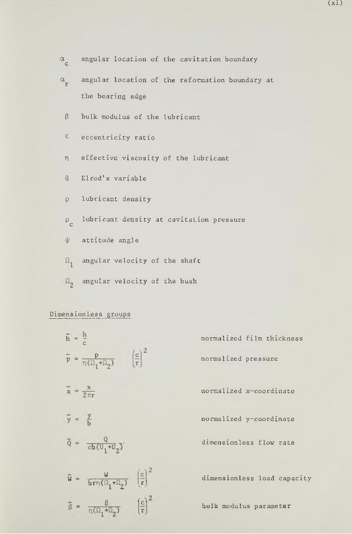
NOMENCLATURE
The following notation is used throughout the thesis,
notation is defined in the sections to which it applies.
a/b groove length-to-bearing width ratio
b bearing width
b/d bearing width—to—bearing diameter ratio
c radial clearance
d bearing diameter
g Elrod's cavitation index
h film thickness
P pressure
pc cavitation pressure
pf lubricant supply pressure
r bearing radius
w/d groove width-to-bearing diameter ratio
X circumferential coordinate
y axial coordinate
cd diametral clearance
Vd clearance ratio
H power loss in ESDU Item No. 66023 (1966)
M number of mesh lines parallel to the bear
N number of circumferential mesh lines
Special

resultant film pressure
component of the resultant film pressure
perpendicular to the line of centres
component of the resultant film pressure f
along the line of centres
lubricant flow rate
flow rate into the cavitation region
theoretical flow rate in ESDU Item No. 66023 (1966)
net flow rate issuing from the groove
pressure induced flow rate in ESDU Item No. 66023 (1966)
flow rate from the bearing sides
velocity induced flow rate in ESDU Item No. 66023 (1966)
flow over the upstream edge of the groove
flow over the downstream edge of the groove
flow over the groove sides (axial direction)
relaxation factor in Gauss-Seidel iteration
speed of rotation of the journal
tangential speed of the shaft surface
tangential speed of the bush surface
load on the bearing
angular coordinate measured from the position of maximum
film thickness in the direction of rotation of the journal
(xi)
ac
angular location of the cavitation boundary
angular location of the reformation boundary at
the bearing edge
3 bulk modulus of the lubricant
£ eccentricity ratio
n effective viscosity of the lubricant
0 Elrod's variable
p lubricant density
p lubricant density at cavitation pressure c
ip attitude angle
angular velocity of the shaft
angular velocity of the bush
Dimensionless groups
h = — normalized film thicknessc
PP normalized pressure
xnormalized x-coordinate
normalized y-coordinate
dimensionless flow rate
2W =
W cr
dimensionless load capacitybrnC ^ + Q ^ )
s cbulk modulus parameter
r

(xii)
Subscripts
amb refers to
c refers to
i refers to
j refers to
x refers to
y refers to
ambient conditions
the cavitation region
nodes on the circumferential mesh line (i)
nodes on the axial mesh line (j)
the circumferential direction
the axial direction

1
CHAPTER 1
INTRODUCTION
The role of lubricants in the reduction of friction between
surfaces in relative motion has been recognised for hundreds of years.
It was, however, the work of Osborne Reynolds in the late nineteenth
century that provided the basis of modern scientific studies of fluid
film lubrication.
Assuming slow viscous flow and a thin film of lubricant,
Reynolds (1886) derived the equation governing the pressure generation
in lubricating films by applying the basic equations of motion and
continuity to the lubricant. For steady-state operating conditions with
an isoviscous, incompressible, lubricant Reynolds' equation can be shown
to reduce to the following commonly used form,
- 6n <u1+u 2 ) | | ( i . D
where (p) is the pressure, (h) is the film thickness, (n) is the dynamic
viscosity of the lubricant, (IL ..U^) are the surface speeds in the (x)
coordinate direction and the axis are chosen such that there are no
surface velocities in the (y) coordinate direction.
In hydrodynamic journal bearings operating under steady-state
conditions the journal does not run concentrically within the bush. The
position of the centre of the journal with respect to the bush centre
_dfh3 | 2 ' 9+ — — h 3
3x 8x 3y 3y » *
2
is dependent on the bearing operating conditions. The eccentricity
between bush and shaft generates the convergent-divergent shape of the
lubricating film observed in journal bearings, making them capable of
supporting loads as a result of the generation of hydrodynamic pressures
in the convergent part of the film.
The determination of the bearing performance is based on a
knowledge of the pressure distribution in the lubricant film in the
bearing, which is obtained by integration of equation (1.1). An
approximate analytical solution of Reynolds' equation may be obtained
by assuming an infinitely wide bearing in which the pressure gradients
in the axial direction are taken equal to zero. Reynolds (1886) has
determined the pressure generated at specific angular locations in an
infinitely wide journal bearing by employing Fourier series to evaluate
some of the integrals involved. This approach was, however, restricted
to values of eccentricity ratio smaller than or equal to 0.5 due to the
requirements for convergence of the series. This difficulty was overcome
by Sommerfeld (1904) with the introduction of a new variable (the
Sommerfeld variable) which made the evaluation of those integrals straight
forward.
The 'short1 journal bearing theory of Dubois and Ocvirk (1953)
has also provided an approximate analytical solution of the Reynolds'
equation which is applicable to bearings of small width-to-diameter
ratio. Short bearing theory assumes that the circumferential pressure
gradients are negligible in comparison with the axial pressure gradients
and is based upon the geometrical condition that the axial length of the
journal bearing is small compared with its, diameter.

3
The results obtained using either of these solutions may,
however, be very inaccurate when applied to realistic bearings. The
width-to-diameter ratio of m o d e m day journal bearings is usually in
the range (0.25-1) and hence the solution of the full Reynolds equation
is required. This can be achieved by numerical analysis and has been
facilitated by the development of digital computers.
The phenomenon known as 'cavitation' usually occurs in the
divergent part of the lubricating film in journal bearings. The most
common type of cavitation encountered in hydrodynamic lubrication is
known as 'gaseous cavitation'. It consists of a disruption of the
continuous film of lubricant by the formation of gas cavities caused
by ventilation from the surrounding atmosphere or by the emission of
dissolved gases from solution when the pressure of the lubricant falls
below the saturation pressure. The disrupted film will reform in the
vicinity of the position where the film profile begins to converge,
depending on the lubricant supply conditions. In the cavitation region,
bounded by the rupture and the reformation boundaries, the pressure is
usually assumed to be constant and equal to the ambient pressure and
Reynolds' equation does not apply. Much attention has been given to the
determination of the rupture boundary and various physical models have
been proposed for its location. This has not been so with the reformation
boundary. Although reformation boundary conditions have been proposed
they have rarely been incorporated in theoretical analyses due to the
complexities arising from the numerical analysis in their implementation.
A widely used film rupture boundary condition is the Reynolds'
boundary condition which assumes that when rupture occurs pressure and
pressure gradients both take the value zero. Many of the journal
bearing design procedures available have been based on solutions of the
4
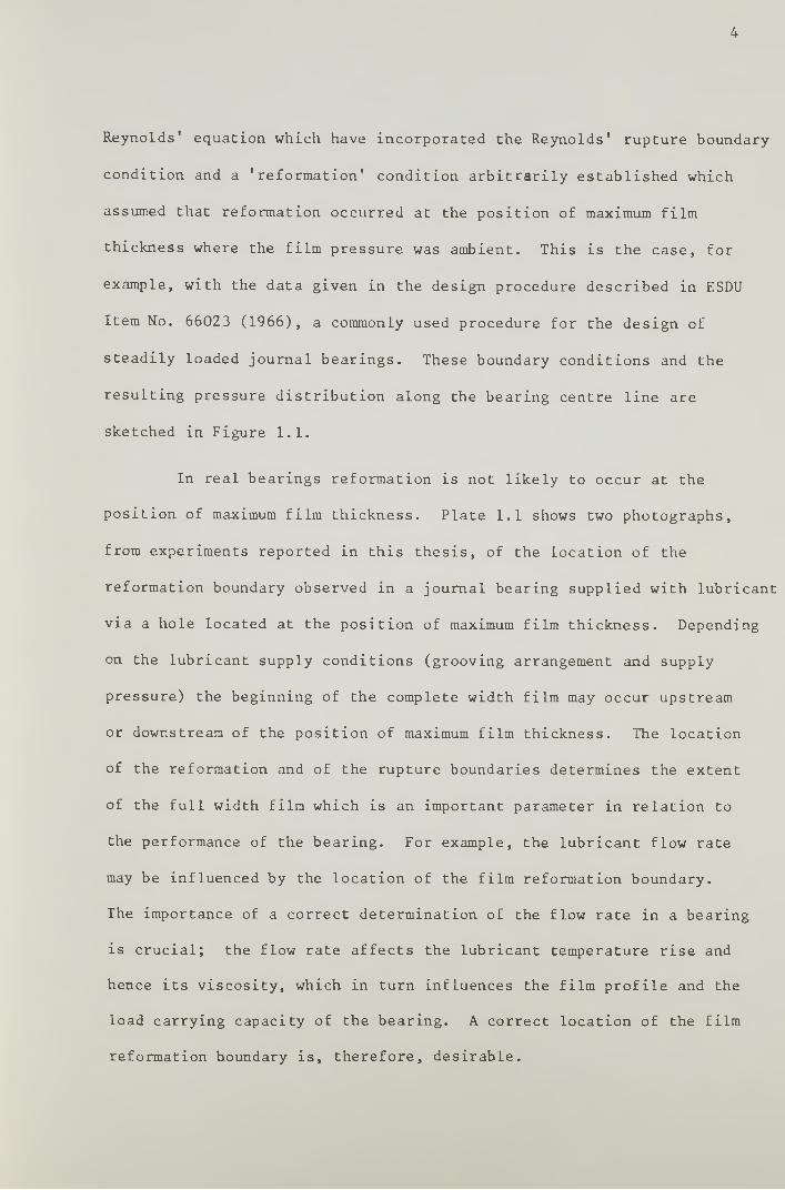
Reynolds' equation which have incorporated the Reynolds' rupture boundary
condition and a 'reformation* condition arbitrarily established which
assumed that reformation occurred at the position of maximum film
thickness where the film pressure was ambient. This is the case, for
example, with the data given in the design procedure described in ESDU
Item No. 66023 (1966), a commonly used procedure for the design of
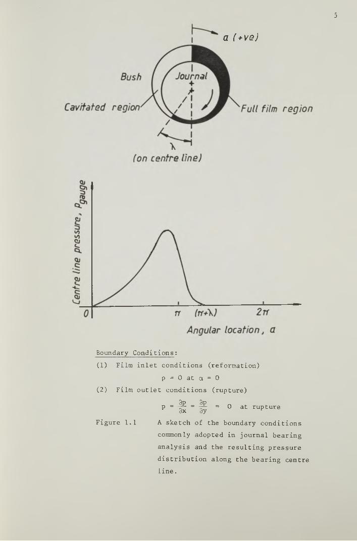
steadily loaded journal bearings. These boundary conditions and the
resulting pressure distribution along the bearing centre line are
sketched in Figure 1.1.
In real bearings reformation is not likely to occur at the
position of maximum film thickness. Plate 1.1 shows two photographs,
from experiments reported in this thesis, of the location of the
reformation boundary observed in a journal bearing supplied with lubricant
via a hole located at the position of maximum film thickness. Depending
on the lubricant supply conditions (grooving arrangement and supply
pressure) the beginning of the complete width film may occur upstream
or downstream of the position of maximum film thickness. The location
of the reformation and of the rupture boundaries determines the extent
of the full width film which is an important parameter in relation to
the performance of the bearing. For example, the lubricant flow rate
may be influenced by the location of the film reformation boundary.
The importance of a correct determination of the flow rate in a bearing
is crucial; the flow rate affects the lubricant temperature rise and
hence its viscosity, which in turn influences the film profile and the
load carrying capacity of the bearing. A correct location of the film
reformation boundary is, therefore, desirable.
5
a (+V6)
Boundary Conditions:
(1) Film inlet conditions (reformation)
p = 0 at a = 0(2) Film outlet conditions (rupture)
3P 3Pp ■ ^ ■ w ■ 0 “ rupture
Figure 1.1 A sketch of the boundary conditions
commonly adopted in journal bearing
analysis and the resulting pressure
distribution along the bearing centre
line.

6
(b)
high 1 ub r i ccu> t
supply pressure
Plate 1.1 Photographs of the location of thefilm reformation boundary in a /journal bearing with oil hole located at the position of maximum film thickness.The direction of shaft rotation was from left to right

7
Elrod and Adams (1974) and Elrod (1981) proposed a computational
algorithm which allowed the automatic determination of the cavitation
region without explicit reference to rupture or reformation boundary
conditions. Mass flow continuity was achieved at the rupture and
reformation boundaries which could be located without encountering the
complexities involved in the implementation of the detailed reformation
boundary conditions as with more conventional numerical analysis
solution schemes.
It was against this background that the present research
programme was established. Its objectives were as detailed below.
Cl) A commonly used procedure for the design of steadily loaded,
fluid film, hydrodynamic journal bearings is described in ESDU
Item No. 66023 (1966). It is a 'hand' type design procedure
which seemed to have much to gain from modern day computing
facilities.
A first objective of the work described in this thesis was the
development of techniques which eventually led to the computerization
of the ESDU Item No. 66023 (1966) design procedure. These techniques
were also expected to be of interest in the computerization of design
procedures of a similar type.
The interactive computer program developed, the techniques
used and the philosophy adopted will be discussed in Chapter 2 of
this thesis.
(2) The second aim of the present research work was to carry out a study
of the effect of film reformation considerations on the performance
of journal hearings, and on the lubricant flow rate in particular.
This investigation was to be initiated for journal bearings having

8
a single axial groove (or oil hole) located at the position of
maximum film thickness. Extension of the investigation to
include more practical grooving arrangements will be a future
priority. To carry out this study the following procedure was
envisaged.
(a) The development of a numerical analysis technique for the
analysis of the performance of journal bearings based on Elrod's
algorithm. Such an approach will enable a detailed study of the
lubricant supply conditions (grooving arrangement and supply
pressure). This will be discussed in Chapter 3.
(b) A comparison of the performance predictions of this analysis
with those of ESDU Item No. 66023 (1966) which did not incorporate
film reformation considerations. This comparative study will be
described in Chapter 4.
(c) The determination of the correlation between the predictions of
the present analysis and experimental measurements. An
experimental apparatus was to be designed and an experimental
programme carried out to provide the results required. The
description of the apparatus will be presented in Chapter 5 and a
discussion of experimental results will be dealt with in Chapter
6.
The overall conclusions of the work undertaken will be presented in
Chapter 7.

9
CHAPTER 2
THE DEVELOPMENT OF AN INTERACTIVE COMPUTER PROGRAM
FOR THE DESIGN OF STEADILY LOADED, LIQUID FILM,
HYDRODYNAMIC PLAIN JOURNAL BEARINGS
2.1 Introduction
With the advent and development of digital computers numerical
analysis techniques acquired new significance and their successful
incorporation into theoretical studies became possible with relative
ease. In the analysis of fluid film bearings in particular, computers
have been used to solve numerically the full Reynolds equation governing
the distribution of pressure within the lubicant film. Computer
solutions for the bearing performance predictions for a wide range of
values of the operating parameters have been made available in the form
of charts of dimensionless quantities, and various 'hand' type design
procedures based on such solutions have been presented by a number of
authors. A good example of this type of design procedure has been
developed by the Engineering Sciences Data Unit (ESDU) and is described
in ESDU Item No. 66023 (1966) - 'Calculation Methods for Steadily Loaded
Pressure Fed Hydrodynamic Journal Bearings'.
'Hand* type bearing design procedures may become tedious and
time-consuming in situations where an iterative procedure is used in
order to reach a satisfactory solution or when an optimized design is
required.

10
Various computer programs for the design of bearings have been
developed in industrial and educational establishments. Taylor (1971)
conducted a survey of existing computerized programs which indicated
the programs available and the gaps that needed to be filled.
A modern trend in the computer-aided design of bearings appears
to be in the application of optimization techniques to the design. In
this context, studies on the optimum design of hydrodynamic journal
bearings have been presented by Seireg and Ezzat (1969) and Dowson and
Ashton (1976).
Computers are not confined to scientific or big business centres.
In recent years, mini- and micro-computers of considerable computing
power which are small in physical size and sufficiently low in price to
make their use acceptable for many applications, have been developed.
In many industrial companies the terms 'computer-aided design (CAD)'
and 'computer-aided manufacture (CAM)' are already familiar and the
tendency to the conversion of 'hand' type design procedures to CAD
techniques is expected to continue. Easy communication between the user
and the computer has been made possible by means of the visual display
unit (VDU) with a keyboard connected directly to the computer. The
user's instructions are typed on the keyboard and the answers of the
computer are displayed on the VDU. Many engineering design requirements
are met by the interactive and the graphics display facilities of
modern computer systems. For computerized bearing design in particular,
these facilities allow an immediate assessment of the effect of changes
in the design parameters on the performance of the bearing making
possible the design of optimized bearings.
Siew and Reason (1982) used both the computer/user interaction
11
and the graphics display facilities in a study of the performance of
hydrodynamic journal bearings. They developed computer programs for
the study of the influence of the boundary conditions adopted, the
lubricant supply pressure and the groove size, on the bearing
performance. The development of computer programs for the analyses of
misaligned journal bearings and porous journal bearings was also
reported.
Most of the existing bearing design computer programs have been
developed to respond to specific needs and are often not suitable for
the use of other consumers. Few interactive computer programs have been
developed and even less (if any) are generally available.
One objective of the work reported in this thesis was the
development of an interactive bearing design computer program based on
the procedure of ESDU Item No. 66023 (1966). This was the most
comprehensive and probably the most commonly used procedure for the
design of hydrodynamic journal bearings.
This chapter includes a brief description of the ESDU Item No.
66023 (1966) procedure and a discussion on the interactive computer
program developed. A more detailed discussion can be found in Miranda
(1983).
2.2 Brief Description of the ESDU Item No. 66023 (1966) Design
Procedure
2.2.1 Major Assumptions
The oomplete assumptions and the limitations of this procedure
are listed on pages 9 and 10 of the document. Only the more important
are dealt with here:

12
(i) The viscosity of the lubricant is assumed to be constant around
the bearing (termed the effective viscosity).
(ii) The maximum lubricant temperature rise in the load carrying part
of the bearing is twice the mean temperature rise. The mean
temperature (effective temperature) is obtained by an iterative
thermal balance and is used to determine the effective viscosity.
(iii) There is no recirculation of lubricant in the bearing. All the
lubricant is assumed to be replaced by fresh lubricant after
having travelled 360° around the bearing.
(iv) The lubricant flow rate in the bearing (Q) is the sum of the
'velocity induced flow rate' (Q^) and the 'feed pressure induced
flow rate' (Qp)• ^or circumferentially grooved bearings (Q )
equals zero.
2.2.2 Design Criteria
The procedure adopted in ESDU Item No. 66023 (1966) ensures a
minimum film thickness at the bearing edge which is safe, and an
acceptable maximum temperature of the lubricant in the bearing.
At low speeds, the minimum film thickness should be large enough
to prevent asperity contacts between bearing and shaft surfaces. At high
speeds, it should be sufficient to prevent the generation of high
temperatures in the region of the minimum film thickness, which can cause
wiping of the bearing metal. Guidance on the safe value of minimum film
thickness is given on Figure 3 of the document.
The limitation on the maximum temperature of the lubricant in the
bearing is required to prevent local melting of the bearing surface.
maximum acceptable temperature is dependent on the particular bearing

13
material employed. For white-metal bearings temperatures up to about
120 C are usually acceptable.
The outlet temperature of the lubricant is used to assess its
susceptibility to oxidation. For mineral oils the critical temperature
is about 75°C when in contact with the atmosphere.
2.2.3 Design Procedure
The procedure of the ESDU Item No. 66023 (1966) allows the
design of both axially and circumferentially grooved bearings and
relies extensively on the use of charts of dimensionless quantities.
Load, speed and bearing diameter are assumed to be design
specifications.
The procedure involves the following stages,
a) The Initial Approximate Design
An initial design chart gives guidance on the selection of the
bearing parameters and the oil type. It may be used to select the
clearance ratio (C^/d), the bearing width-to-bearing diameter ratio (b/d)
and the oil characteristics. An estimation of the effective viscosity
of the oil can also be obtained and used as a starting value in the
thermal iteration to determine the effective viscosity. A load capacity
chart (Figure 6 of the document) allows the determination of the
operating eccentricity ratio (e) and a check for operation within the
'Recommended Area'. This is a region bounded by curves of maximum and
minimum recommended values of (b/d) (1.25 and 0.2 respectively), and
by limiting maximum and minimum loading conditions for a given value of
(b/d). Lightly loaded journal bearings are prone to instability but
this will not normally occur if the operating point is within the
'Recommended Area'.
14
b) The Full Design
Having selected the bearing parameters and the oil type, the
effective viscosity of the oil is required to calculate the bearing
performance characteristics.
The effective temperature is obtained from a thermal balance
involving the lubricant flow rate, the power loss and the temperature
rise in the bearing. Due to the interconnection between these three
quantities an iteration is usually required to calculate the effective
operating temperature.
Because of the assumption made regarding lubricant recirculation
around the bearing (Section 2.2.1 -(iii)) the primary aim of this
procedure is to provide a full width film of lubricant at the groove
location whenever possible. A theoretical flow rate (Q_), required to
fill completely the clearance space at the groove, is determined, and the
iteration to calculate the effective temperatue is performed involving
the flow (Q ) and the power loss (H). The groove size is then selected,£
and the lubricant supply pressure required to provide a flow rate in the
bearing (Q) such that Q i Q is then calculated. If the supply pressureu
required for fully flooded conditions (Q ^ Q ) is too high, the bearing
has to be designed for a flow (Q) smaller than the theoretical flow
(Q ) - the bearing is termed 'starved'. In such a case the effective £
viscosity of the lubricant and the performance characteristics of the
bearing have to be recalculated.
c) The Performance Characteristics
If some of the calculated values of the performance characteristics
of the hearing are not acceptable, guidance is given on which parameters
should be altered, and in what direction, to achieve acceptable operating
15
conditions. However, a considerable effort and a careful selection of
parameters and determination of the corresponding bearing performance,
would be required to design an optimized bearing.
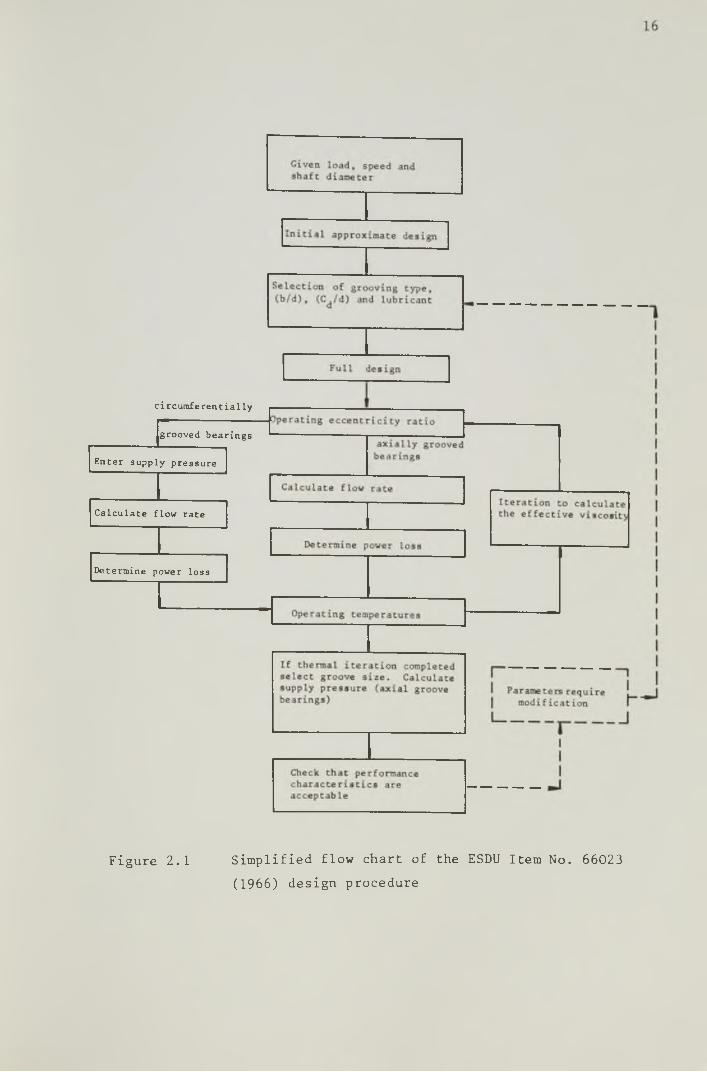
Figure 2.1 shows a simplified flow chart of the ESDU Item No.
66023 (1966) design procedure.
2.3 Discussion of an Interactive Computer Program for the Design of
Steadily Loaded Hydrodynamic Journal Bearings
Originally, it was intended to develop a program that followed
exactly the procedure of the ESDU Item No. 66023 (1966) . In its original
version, in fact, the program developed followed very closely the
philosophy adopted in that document and made extensive use of design
charts. An optimization facility was already included in this version.
The program was mounted on the VAX 11/780 Computer in the
Department of Mechanical Engineering in the University of Leeds. The
language used was Fortran IV and the software involved was the GINO-F
Graphics Package.
Not all the diagrams of the ESDU Item No. 66023 (1966) were
reproduced on the V.D.U. screen, some were substituted by data stored
in tabular form. Graphical interaction was possible by using the cursor
mechanism and interpolation routines were used for interpolation in
table functions.
A subsidiary program was written which produced the diagrams
required in a special code form. The output of this program was stored
in a data file, constituting a library of diagrams that could be used by
the design program.
A change in philosophy with respect to the approach employed at
some particular points of the design procedure was implemented after
circuraferentially
grooved bearings
Enter supply pressure
Calculate flow rate
Determine power loss
Figure 2.1 Simplified flow chart of the ESDU Item No. 66023
(1966) design procedure

17
discussions with, interested academics and industrialists, and different
computer strategies, suggested by the experience of using the original
version of the program, were adopted.
It was recognized that the use of diagrams, although being a
suitable means of presenting some design features and valuable for less
experienced users, nevertheless increased both the time and the storage
space required for running the program.
Two new versions resulted from the development of the original
form of the computer program:
(1) A graphics version, which employed charts 2B , 6 , 12 and 13 of
the ESDU Item No. 66023 (1966) and which was able to generate
diagrams showing the effect of changes in the parameters on the
performance of the bearing. As an alternative to graphical inter
action, this version also provided the possibility of using internal
calculations from data in tabular form. At the beginning of the
program a switch existed which permitted the selection of the
graphics or the non-graphics option, according to the type of
terminal being used. A Tektronix 4014 terminal was required to run
the graphics version of the program under the graphics option.
(2) A non-graphics version, which did not use any diagrams. The
procedure followed in this version was similar to that of the
graphics version running on the non-graphics option. The reason
why this was developed as a separate program was the recognition
that such a program would require less memory space and could be a
useful version for experienced designers or whenever a suitable
graphics terminal was not available.
The two versions of the program were not different in their structure and
therefore there is no need to consider them separately.
18
2.3.1 Selection of the Bearing Parameters
Load and speed were assumed to be design specifications. The
bearing diameter, when it was not specified or calculated by strength
considerations, was estimated by the program and could be altered at a
later stage of the design, if required. The value provided was in the
range (25-500 mm) and was obtained according to Figure 5, Section A5 of
the Tribology Handbook (1973), assuming b/d = 0.75.
Clearance ratio (C^/d), bearing width-to-bearing diameter ratio
(b/d) and lubricant characteristics, were either inputted directly to
the program or selected using the initial design chart. Guidance was
given on the chart and the associated instructions for the selection
of the parameters.
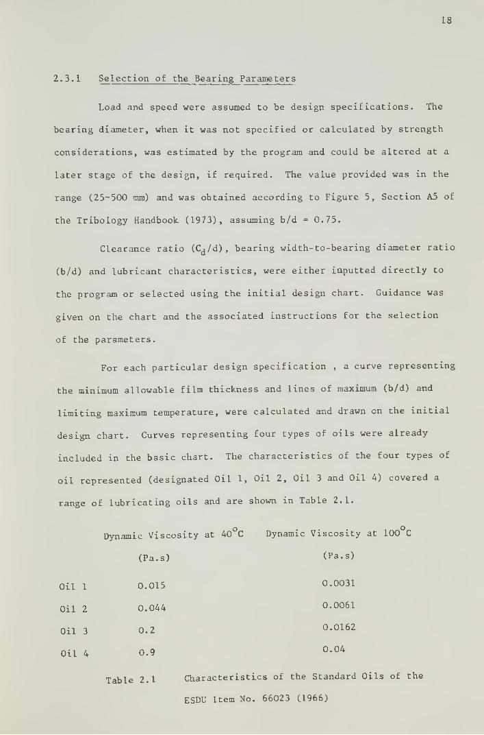
For each particular design specification , a curve representing
the minimum allowable film thickness and lines of maximum (b/d) and
limiting maximum temperature, were calculated and drawn on the initial
design chart. Curves representing four types of oils were already
included in the basic chart. The characteristics of the four types of
oil represented (designated Oil 1, Oil 2, Oil 3 and Oil 4) covered a
range of lubricating oils and are shown in Table 2.1.
Dynamic Viscosity at 40°C Dynamic Viscosity at 100°C
(Pa.s) (Pa.s)
Oil 1 0.015 0.0031
Oil 2 0.044 0.0061
Oil 3 0.2 0.0162
Oil 4 0.9 0.04
Table 2.1 Characteristics of the Standard Oils of the
ESDU Item Nov 66023 (1966)

19
The computer program allowed the consideration of any other
oil along with the standard oils of the ESDU Item No. 66023 (1966).
The curve corresponding to this non-standard oil was calculated and
drawn on the initial design chart. To perform this calculation the
effect of temperature variations on both viscosity and density was
considered, and the values of the kinematic viscosity of the oil at
40 C and 100°C, as well as the oil density at a given temperature,
were required.
An approximate value of the effective viscosity of the lubricant
in the bearing was also obtained from the initial design chart for
the design selected. If the alternative of entering the bearing parameters
directly was chosen, the oil type and an estimation of the effective
temperature of the oil, would be required.
A first check for operation within the 'Recommended Area' was
carried out and, if the design was acceptable, the approximate bearing
performance characteristics were printed out. Re-selection of the
bearing parameters was possible until acceptable operating conditions
were reached.
2.3.2 Lubricant Supply Pressure and the Design of the Groove (Axial
Groove Bearings)
The primary objective of the ESDU Item No. 66023 (1966) procedure
is to achievefully flooded conditions as discussed in Section 2.2.3.
The groove size is selected, and the lubricant supply pressure
calculated, to provide a full width film of lubricant at the groove
location. The maximum acceptable value for supply pressure is
2considered to be 350 kN/m .
20
A different approach was adopted in the computer program
being described. In modern day bearing design lubricant supply
2 2 pressures of 50 kN/m are common practice and 150 kN/m is considered
to be a high supply pressure (Martin (1981)). Thus, perhaps fifty
per cent of hydrodynamic bearings operate with 'starved1 conditions.
The program provided two alternatives for the design of the
groove and the calculation of the supply pressure:
(i) To select the groove size and calculate the lubricant supply
pressure for full flow. Changes in the size of the groove
were allowed until the value of the supply pressure was
considered to be acceptable.
(ii) To select both the groove size and the supply pressure without
reference to fully flooded conditions. The degree of
starvation (if appropriate) and the performance characteristics
of the bearing were then calculated.
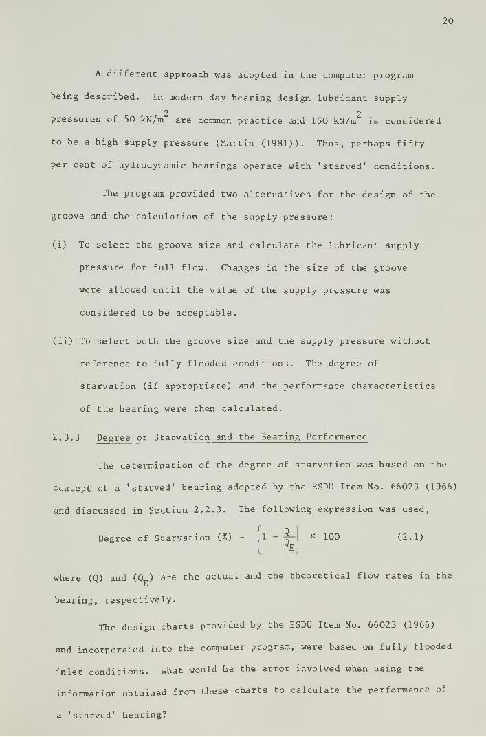
2.3.3 Degree of Starvation and the Bearing Performance
The determination of the degree of starvation was based on the
concept of a 'starved' bearing adopted by the ESDU Item No. 66023 (1966)
and discussed in Section 2.2.3. The following expression was used,
QDegree of Starvation (%) =
' Qex 100 (2 .1)
where (Q) and (Q ) are the actual and the theoretical flow rates in the E
bearing, respectively.
The design charts provided by the ESDU Item No. 66023 (1966)
and incorporated into the computer program, were based on fully flooded
inlet conditions. What would be the error involved when using the
information obtained from these charts to calculate the performance of
a 'starved' bearing?

21
Connors (1962) has presented design charts for b/d = 1 where
incomplete inlet film conditions were taken into account. Values of
the performance characteristics of the bearing calculated using the
computer program were compared with those obtained using Connors' design
charts. The lubricant flow rates considered were those predicted by
the computer program. A bearing with the following characteristics
was considered:
Load = 6000 N
Speed = 1200 r.p.m. (20 Hz)
Diameter = 100 m m
Width-to-diameter ratio (b/d) = 1
Clearance ratio (C /d) = 0.002a
Standard oil No. 2 (ESDU Item No. 66023 (1966))
Oil supplied at atmospheric pressure
Axial groove at the position of maximum film thickness
Groove width-to-bearing diameter ratio (w/d) = 0.15
The groove length-to-bearing width ratio (a/b) was varied
in the range (0.3 - 0.9) to provide variable degrees of
starvation.
The computed degree of starvation varied from 53.7% (at a/b = 0 . 9 ,
e = 0.42) to 82.1% (at a/b = 0.3, e = 0.51).
The results obtained using Connors' procedure showed smaller
values of minimum film thickness, slightly higher maximum temperatures
(l_2°c higher) and lower power loss (about 12%), for all degrees of
starvation.
The discrepancy observed in minimum film thickness increased
from 5.2% at the degree of starvation of 53.7%, to 29.2% with 82.1%

22
starvation. These results show that there are limitations on the use
of the ESDU Item No. 66023 (1966) procedure with high degrees of
starvation, but seemed to sugges t that this procedure was acceptably
accurate with degrees of starvation up to about fifty per cent.
2.3.4 The Bearing Optimization
After the groove size and the supply pressure had been selected,
a thermal iteration was performed to calculate the effective viscosity
of the lubricant. Final checks for operation within the 'Recommended
Area' and for laminar flow conditions, were then carried out.
The bearing parameters selected and the performance characteristics
calculated were all printed out on the V.D.U. screen.
In many applications it might be important to minimize power loss,
or flow rate, keeping mini mum film thickness and maximum temperature
at acceptable levels. Any change in a particular bearing parameter will
affect the whole performance of the bearing and some compromise has
to be adopted by the designer between the desirable and the acceptable.
To give the designer an immediate assessment of the effect of
changes in one or more parameters on the performance of the bearing,
an optimization procedure was incorporated in the computer program.
a) Effect of Individual Changes in the Parameters
The effect of individual changes in diameter, bearing width,
diametral clearance and oil type, on minimum film thickness, oil flow
rate, power loss and maximum temperature, was calculated and shown in
graphical form. The plots of the variation of minimum film thickness
also included the safe minimum film thickness curve in the domain
defined for the variation of the parameter. The maximum allowable
temperature curve was also represented on the diagrams showing the effect

23
of changes of a given parameter on maximum bearing temperature.
The domain of variation of the parameter under consideration
was defined by the designer and inputted to the program as a
fractional change with respect to the value selected in the full
design, which was the central point in the field of variation.
b) Effect of Combined Changes in the Parameters on the Bearing
Performance
Having studied the effect on the performance of the bearing of
individual changes in the parameters, the effect of combined changes
could be determined, if required. Only the parameters mentioned in a)
and the oil type were allowed to be changed. The groove size and the
oil supply pressure were kept unchanged at the values selected in the
full design. The performance predictions were shown in tabular form.
There was no limitation in the number of combinations of
parameters that could be considered.
Once it had been decided what alterations to adopt, if any,
the new values of the parameters and the oil type were inputted and
the bearing performance was re—calculated. Checks for operation within
thg 'Recommended Area* and laminar flow conditions were carried out for
the new operating conditions, and the performance characteristics of
the optimized bearing were printed out.
2.3.5 The Load-Speed Diagram
Bearing load and shaft speed were assumed to be design
specifications. In operation, however, 'off-design' loads or speeds
may sometimes occur.
To provide information relating to the effect of ’off-design’
conditions on critical performance parameters, such as minimum film

24
thickness and maximum lubricant temperature, the program was able to
calculate and draw a load-speed diagram of the bearing designed. If
a graphics facility was not available, the load-speed characteristics
of the bearing were shown in the form of pairs of values for load and
speed representing points on the load-speed curve.
Figure 2.2 shows a sketch of a typical load-speed diagram. The
curve is composed of two portions:
(a) The minimum film thickness portion, is defined by pairs (load,
speed) such that the minimum film thickness at the bearing edge
is equal to the safe minimum film thickness. At a given speed
(S), the maximum allowable load to ensure that the minimum film
thickness is safe, is (W ). For a given load (W), the minimum
speed that ensures a safe minimum film thickness is (S^).
(b) The maximum temperature portion, is the locus of points corresponding
to operating conditions such that the maximum temperature of the
lubricant equals the maximum allowable temperature. At a given
operating speed (S£), the maximum allowable load to prevent an
excessive temperature rise is (W„), and at a given load (W), the
maximum speed permitted is (S_).
Operating points within the region below the curve will
represent safe operating conditions with respect to minimum film
thickness and maximum lubricant temperature.
2.3.6 The Program' Flow Chart
The structure of the program was somewhat complex due to the
numerous calculations involved and the various alternatives offered to
the designer anytime a decision was required.

25

2 6
The graphics version of the program used sixteen routines and
had additional complexities connected with the use of charts and
graphical interaction. A detailed flow chart is available in Miranda
(1983).
A very simplified program flow chart is shown in Figure 2.3.
In broad terms, the procedure could be divided into four parts:
(1) The bearing specifications and the selection of parameters
(2) The determination of the effective viscosity of the lubricant
(3) The design of the groove and the calculation of the lubricant
supply pressure (Axially grooved bearings)
(4) The optimization process
In part (3), a significant change in philosophy with respect to
the ESDU Item No. 66023 (1966) procedure was adopted. The approach
employed and its implications have been dealt with in Sections 2.3.2
and 2.3.3.
Bearing design procedures of the 'hand' type are usually not
orientated to the design of optimized bearings. This was the case of
the procedure described in ESDU Item No. 66023 (1966), although
improvements in the design could be made by sensibly changing the
bearing parameters. It is the computerization, however, that provides
the conditions for an optimization study to be carried out. Such a
study was included in the computer program procedure and constituted
an important design aid.
2.3.7 Complete Sequence of Pages Produced on the V.D.U. Screen When
Running the Graphics Version of the Program
The following example illustrates the use of the program. The
design specifications are listed below and the computer output follows.

27
Enter load and speed
Enter/calculate diameter
APPROXIMATE DESIGN
Select grooving type, bearing parameters and lubricant
| Alter parameters until . initial design is I acceptable '
FULL DESIGN
( cir curaf e rent iall)
grooved bearings
Thermal iteration to calculate the effective viscosity of the lubricant (with axially grooved bearings full flow is assumed)
1■H-----------------------------------■ Calculation ofI eccentricity ratio, flow| rate, power loss,| effective temperature
____________________ I(axially grooved bearings)
Groove size/lubricant supply pressure1 - Select groove size and
calculate supply pressure for full flow
2 - Select groove size and supplypressure
Recalculate effective viscosity and performance characteristics
Check for laminar flow and 'Recommendedoperation within
Area'
" 1Print out bearing parameters and performance characteristics.Draw load-speed diagram (if required)
OPTIMIZATION
Study of the effect of changes in the parameters on the bearing performance.
•C si°p )
Enter optimized parameters (if appropriate)
Figure 2.3 Simplified program flow chart

28
Load = 1000 N
Shaft speed ■ 1000 r.p.m. (16.66 Hz)
Diameter = 50 mm
Maximum bearing width = 80 mm
-3Angular misalignment = 0.1 x 10 mm/mm
Allowable maximum temperature = 100°C
Inlet oil temperature = 40 C
It is required to consider the possibility of using the
SAE 30 engine oil, with the following characteristics:
Kinematic viscosity at 40°C = 112.7 cSt (112.7 x 10 m /s)
o “6 2Kinematic viscosity at 100°C = 12.52 cSt(12.52 x 10 m / s)
Density at 40 C = 875 Kg/m
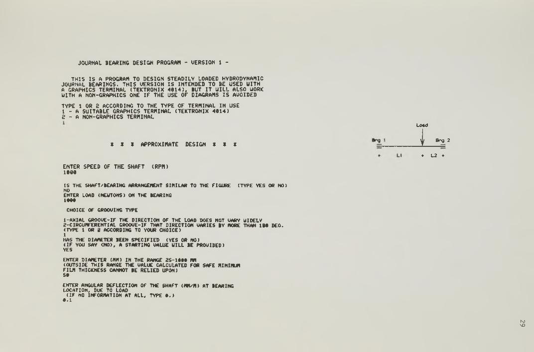
JOURNAL BEARING DESIGN PROGRAH - VERSION 1 -
THIS IS A PROGRAM TO DESIGN STEADILY LOADED HYDRODYNAMIC JOURNAL BEARINGS. THIS UERSION IS INTENDED TO BE USED UITH A GRAPHICS TERMINAL (TEKTRONIX 4014). BUT IT UILL ALSO UORK UITH A NON ■'GRAPHICS ONE IF THE USE OF DIAGRAMS IS AUOIDED
TYPE 1 OR 3 ACCORDING TO THE TYPE OF TERMINAL IN USE1 - A SUITABLE GRAPHICS TERMINAL (TEKTRONIX 4014) a - A NON-GRAPHICS TERMINAL
X X X APPROXIMATE DESIGN X X X
ENTER SPEED OF THE SHAFT (RPM) 1000
IS THE SHAFT/BEARING ARRANGEMENT SIMILAR TO THE FIGURE (TYPE YES OR HO) NOENTER LOAD (NEWTONS) ON THE BEARINO 1000
CHOICE OF GROOVING TYPE
1-AXIAL CR00VE-1F THE DIRECTION OF THE LOAD DOES NOT VARY UIDCLY2-CIRCUMFERENTIAL GROOVE-IF THAT DIRECTION VARIES BY MORE THAN 1B0 DEO. (TYPE 1 OR 2 ACCORDING TO YOUR CHOICE)1HAS THE DIAMETER BEEN SPECIFIED (YES OR NO)(IF YOU SAY <N0>, A STARTING UALUE UILL BE PROVIDED)YES
ENTER DIAMETER (MM) IN THE RANGE 2S-1000 HH(OUTSIDE THIS RANGE THE UALUE CALCULATED FOR SAFE MINIMUMFILM THICKNESS CANNOT BE RELIED UPON)SO
ENTER ANGULAR DEFLECTION OF THE SHAFT (MM/M) AT BEARING LOCATION, DUE TO LOAD (IF NO INFORMATION AT ALL* TYPE 0.)
0.1
Load
V Br± 2
♦ L2 ♦
hovo
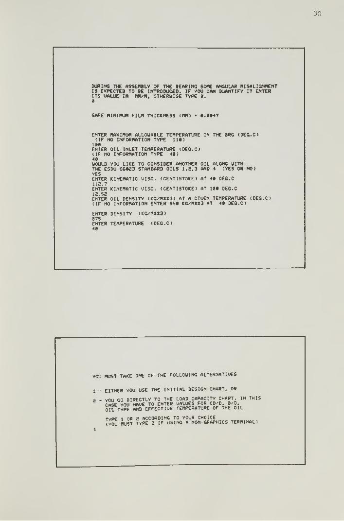
30
DURING THE ASSEMBLY OF THE BEARING SOME ANGULAR MISALIGNMENT IS EXPECTED TO BE INTRODUCED. IF YOU CAN QUANTIFY IT ENTER ITS VALUE IN msn, OTHERWISE TYPE 9.9
SAFE NINIHUH FILM THICKNESS (UN) • 9.9*47
ENTER MAXIMUM ALLOUABLE TEMPERATURE IN THE BRG (DEG.C)(IF NO INFORMATION TYPE 119)100
ENTER OIL INLET TEMPERATURE (DEG.C)I IF NO INFORMATION TYPE 49)49WOULD YOU LIKE TO CONSIDER ANOTHER OIL ALONG WITH THE ESDU 66923 STANDARD OILS 1.2.3 AND 4 (YES OR NO)YESENTER KINEMATIC VISC. (CENTISTOKE) AT 49 DEG.C112.7ENTER KINEMATIC VISC. (CENTISTOKE) AT 199 DEG.C 12.52ENTER OIL DENSITY (KG/^1**3) AT A GIVEN TEMPERATURE (DEG.C) (IF NO INFORMATION ENTER 8S9 K G / M M 3 AT 49 DEG.C)
ENTER DENSITY (KG/NSt3)875ENTER TEMPERATURE (DEG.C)49
YOU MUST TAKE ONE OF THE FOLLOWING ALTERNATIVES
1 - EITHER YOU USE THE INITIAL DESIGN CHART. OR
a - YOU GO OIRECTLY TO THE LOAD CAPACITY CHART. IN THIS rA<r YOU HAVE TO ENTER VALUES FOR CD^D. B^D.OIL TYPE AND EFFECTIVE TEMPERATURE OF THE OIL
TYPE 1 OR 2 ACCORDING TO VOUR CHOICE(YOU MUST TYPE 2 IF USING A NON-GRAPHICS TERMINAL)
1

32
SELECTED CD/D- 0.00119
SELECTED B/D • 0.508
DUE TO INACCURACY UHEN USING THE CURSOR THESE VALUES BE SLIGHTLY DIFFERENT FROM UHAT YOU HAVE INTENDED TO
NAYSELECT
UOULD YOU LIKE TO CORRECT THEH (YES OR NO) YES
ENTER CORRECT CD/D .0012
ENTER CORRECT B/D .S

CHECKING IF THE DESIGN SELECTED UILL OPERATE UITHIN THE RECOMMENDED REGION
TAKE ONE OF THE FOLLOWING ALTERNATIVES
t - THE USE OF A LOAD CAPACITY CHART ENABLING A CHECK OF THE OPERATING POINT UITH RESPECT TO A RECOMMENDED AREA OF OPERATION
2 - NO DIAGRAM AVAILABLE. THE CHECK BEING HADE BY INTERNAL CALCULATIONS. GUIDANCE UILL BE GIVEN FOR CRITICAL OPERATING CONDITIONS
TYPE 1 OR 2 ACCORDING TO YOUR CHOICE(YOU MUST TYPE 2 IF USING A NON-GRAPHICS TERMINAL)1
B/D • *.5«
CHECKING IF THE DESIGN FALLS INSIDE THE RECOMMENDED AREA
PROCEDURE TO BE FOLLOUED
1-MOVE HORIZONTAL CURSOR LINE TO SYMBOL ♦2-MOVE VERTICAL LINE TO THE INTERSECTION OF THE B/D CURVE
UITH THE HORIZONTAL CURSOR LINE3-PRESS KEY (E)
DO YOU CONSIDER IT ACCEPTABLE AT THIS STAGE (YES OR NO) YES
.2haifv'cd
.1 .* .6 .1Ecc.Ratio

34
INITIAL APPROXIHATE DESIGN
D B'D CD/D ECC TflAX h u i n HSAFE(rtfl) (DEG.C) (fin) (Nfl)
50. 0.50 0.0012 0.56 60.6 0.012 0.005
TO CONTINUE, PRESS <RETURN)
* » * FULL DESIGN X X X
ENTER (HEAT CAPACITY * DENSITY/10X*6) FOR THE LUBRICANT (SI UNITS)(IF NO INFORMATION, TYPE 1.7 FOR OILS, AND 4.2 FOR WATER)1.7
ENTER THE PROPORTION K OF HEAT GENERATED IN THE BEARING TRANSFERRED TO THE LUBRICANT(IT IS USUALLY SUFFICIENTLY ACCURATE TO TAKE IC-0.8)0.8
CHOICE OF GROOUE POSITION
1-SINGLE AXIAL GROOVE (OR HOLE) AT HNAX.- IT IS THE ROST FAVOURABLE LOCATION. BUT THE POSITION OF HMAX. VARIES UITH LOAD AND SPEED. SO IT IS ONLY UELL DEFINED FOR CONSTANT OPERATING CONDITIONS
2-SINGLE AXIAL GROOVE (OR HOLE) AT 90 DEG TO THE LOAD LINE - SUITABLE FOR SPLIT BEARINGS UITH CONSTANT DIRECTION OF ROTATION
3-TUO DIANETRALLY OPPOSED AXIAL GROOVES (OR HOLES) AT 90 DEG TO THE LOAD LINE - CONVENIENT FOR MANUFACTURE AND ASSEMBLY. ALLOUS ROTATION IN EITHER DIRECTION
TYPE 1,2 OR 3 ACCORDING TO YOUR CHOICE1
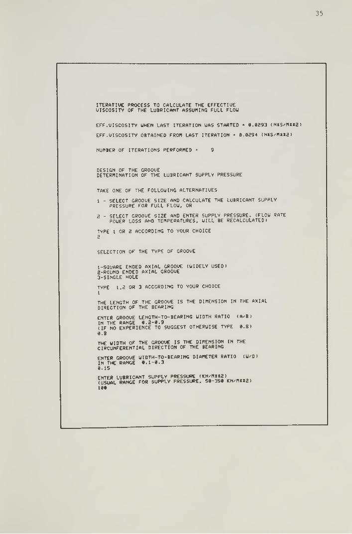
35
ITERATIVC PROCESS TO CALCULATE THE EFFECTIVE UISCOSITY OF THE LUBRICANT ASSUMING FULL FLOU
EFF.UISCOSITY UHEN LAST ITERATION UAS STARTED • 0.9293 (NSS/NM2)
EFF.UISCOSITV OBTAINED FROM LAST ITERATION • 0.0294 (N*S/MK2)
NUHBER OF ITERATIONS PERFORMED • 9
DESIGN OF THE GROOUEDETERMINATION OF THE LUBRICANT SUPPLV PRESSURE
TAKE ONE OF THE FOLLOWING ALTERNATIUES
1 - SELECT GROOUE SIZE AND CALCULATE THE LUBRICANT SUPPLVPRESSURE FOR FULL FLOU, OR
2 - SELECT GROOUE SIZE AND ENTER SUPPLV PRESSURE. (FLOU RATEPOUER LOSS AMD TEMPERATURES, UILL BE RECALCULATED)
TYPE t OR 2 ACCORDING TO VOUR CHOICE2
SELECTION OF THE TYPE OF CROOVE
1-SQUARE ENDED AXIAL GROOUE (UIDELV USED)2-ROUND ENDED AXIAL GROOUE3-SINGLE HOLE
TYPE 1,2 OR 3 ACCORDING TO VOUR CHOICE1THE LENGTH OF THE GROOUE IS THE DIMENSION IN THE AXIAL DIRECTION OF THE BEARING
ENTER GROOUE LENGTH-TO-BEARING UIDTH RATIO (A/B)IN THE RANGE 0.2-9.9(IF NO EXPERIENCE TO SUGGEST OTHERUISE TYPE 9.8)9.8
THE WIDTH OF THE GROCUC IS THE DIMENSION IN THE CIRCUNFERENTIAL DIRECTION OF THE BEARING
ENTER GROOUE UIDTH-TO-BEARIHC DIAMETER RATIO (U'D)IN THE RANGE 9.1-9.3 9.IS
ENTER LUBRICANT SUPPLY PRESSURE (KN/MIJ2)(USUAL RANGE FOR SUPPLY PRESSWJE. S9-3S9 K N / M M 2 )199
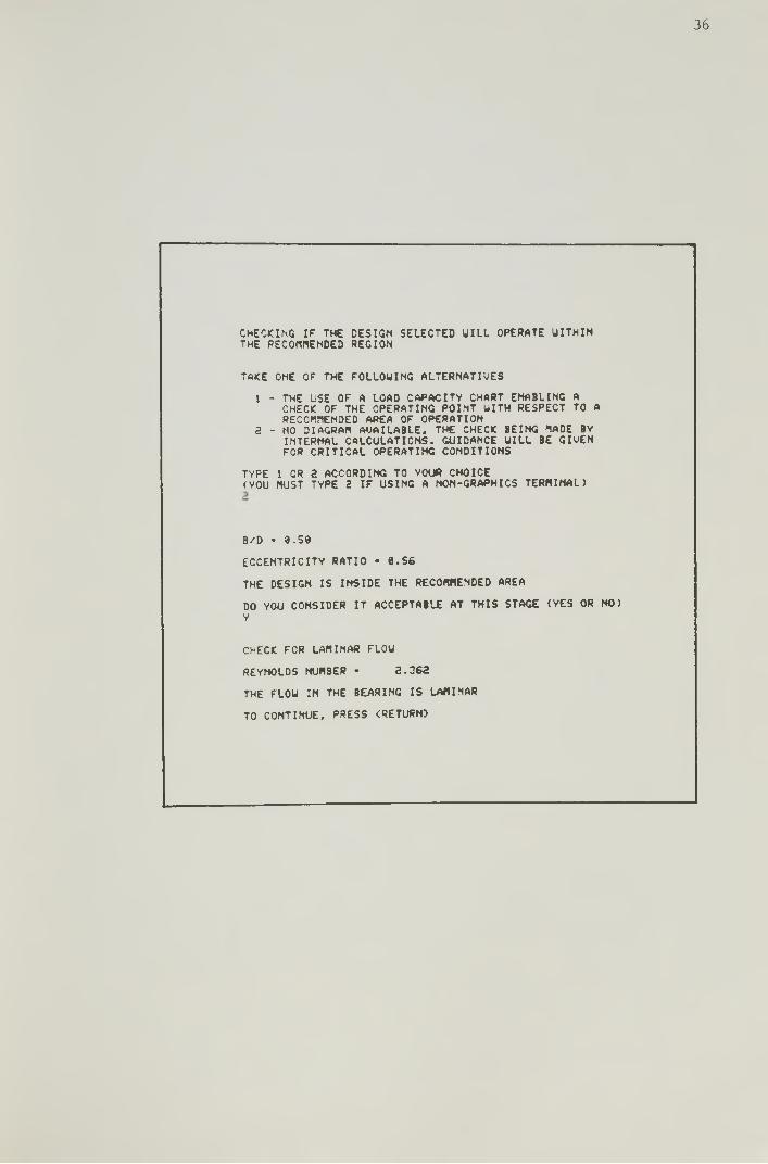
36
CHECKING IF THE DESIGN SELECTED U I U OPERATE UITHIN THE RECOMMENDED REGION
TAKE ONE OF THE FOLLOWING ALTERNATIVES
1 - THE USE OF A LOAD CAPACITY CHART ENABLING ACHECK OF THE OPERATING POINT UITH RESPECT TO A RECOMMENDED AREA OF OPERATION
2 - NO DIAGRAM AVAILABLE, THE CHECK BEING MADE BYINTERNAL CALCULATIONS. GUIDANCE UILL BE GIVEN FOR CRITICAL OPERATING CONDITIONS
TYPE 1 OR 2 ACCORDING TO YOUR CHOICE(YOU MUST TYPE 2 IF USING A NON-GRAPHICS TERMINAL)
B/D • 0.59
ECCENTRICITY RATIO • 0.S6
THE DESIGN IS INSIDE THE RECOMMENDED AREA
DO YOU CONSIDER IT ACCEPTABLE AT THIS STAGE (YES OR NO)Y
CHECK FOR LAMINAR FLOU
REYNOLDS NUMBER * 2.362
THE FLOU IN THE BEARING IS LAfllNAR
TO CONTINUE. PRESS <RETURN>

DESIGN PARAMETERS OF THE BEARING
BEARING DIAMETER (MM) ■ 5®-*
BEARING UIDTH (NM) ■ 26.#
DIAMETRAL CLEARNCE (MM) • •
LUBRICANT SUPPLY PRESSURE (KN/MME) • 1 M . M
LUBRICANT CHARACTERISTICS <
KINEMATIC UISCOSITV (CENTISTOKE) AT 4» DEG.C • 61.76 KINEMATIC UISCOSITV (CENTISTOKE) AT I N DEG.C • 6.84
SINGLE SQUARE ENDED AXIAL GROOVE AT HRAX.
LENGTH OF THE CROOUE (NR) • 2«.B
UIDTH OF THE CROOUE (MM) • 7.5
PERFORMANCE CHARACTERISTICS
THE BEARING IS 27.6 X STARVED
ECCENTRICITY RATIO • ».56
MINIMUM FILM THICKNESS AT THE EDGE (MM) • •.•120
TOTAL POUER LOSS (UATTS) * 24.86
TOTAL FLOU RATE OF LUBRICANT ( N»3/S> -
LUBRICANT OUTLET TEMPERATURE (DEG.C) • S*.9
MAXIMUM TEMPERATURE (DEG.C) • 67.8
ATTITUDE ANGLE (DEG) • SI.2
tt SAFE MINIMUM FILM THICKNESS (NM) • A . M 4 7 (THE SAFETY FACTOR USED UAS 2)IF ONLY LIMITED ATTENTION HAS BEEN PAID TO MISALIGNMENT CONSIDERATIONS A LARGER SAFETY FACTOR NAY BE APPROPRIATE (UITH A SAFETY FACTOR OF 3. MMIN.SAFE BASED ON THE SURFACE ROUGHNESS CRITERION, IS « . M 7 « MM)
t* MAXIMUM ALLOWABLE TEMPERATURE (DEG.C) • 1 M . 0 H ASSUMED OIL INLET TEMPERATURE (DEG.C) • 4*.*
IS OPTIMIZATION REQUIRED (YES OR NO) YES
DO YOU UISH TO LOOK AT THE LOAD-SPEED CHARACTERISTICS OF THE BEARING DESIGNED (YES OR NO) YES
TYPE 1 OR 2 ACCORDING TO YOUR CHOICE
1 - SHOUN IN THE FORM OF A DIAGRAM2 - IN A TABULAR FORM(YOU MUST TYPE 2 IF USING A NON-GRAPHICS TERMINAL) 1
SPEED < r p n )
LO AO -SPEED DIAGRAM

OPTIMIZATION PROCESS
IF REQUIRED IT UILL BE POSSIBLE TO SEE THE EFFECT OF A CHANCE IN D, B, CD OR OIL TYPE UPON THE BEARING PERFORMANCE. FOR THE SPECIFIED LOAD AND SHAFT SPEED, AND SELECTED GROOUE SIZE AND OIL SUPPLV PRESSUREIT UILL ALSO BE POSSIBLE TO CONSIDER COMBINED CHANGES OF THOSE PARAMETERS
UOULD YOU LIKE TO SEE THE EFFECT OF A CHANGE IN D (YES OR NO)Y
ENTER FRACTIONAL CHANCE IN D TO EITHER SIDE OF THE SELECTED UALUE. <EC. 0.1. 0.2S. ETC.)0.2
THE DIAGRAMS SHOU THE EFFECT ON THE BRG PERFORMANCE OF ACHANGE IN D ALONE
TO CONTINUE. PRESS <RETURN>
r t * x . tF W > S R A IU S £ ( 0* « . C >
o o o r u X . ALLO W ABLE
«s|-I
CO00
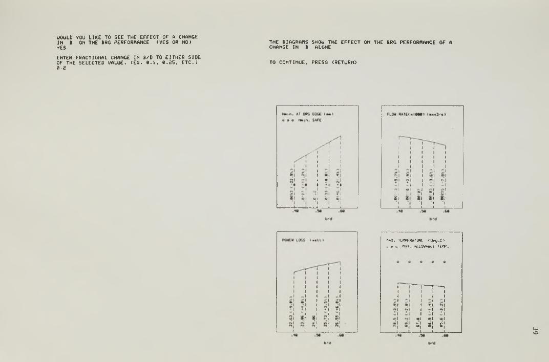
UOULD YOU LIKE TO SEE THE EFFECT OF A CHANGE IN B ON THE BRG PERFORMANCE (YES OR NO)YES
ENTER FRACTIONAL CHANCE IN B/D TO EITHER SIDE OF THE SELECTED UALUE. (EC. 0.1, 0.25, ETC.) 0.2
TO CONTINUE, PRESS <RETURN>
THE DIAGRAMS SHOU THE EFFECT ON THE BRG PERFORMANCE OF ACHANGE IN B ALONE
n*K. r c r P F M T U R E <0*g.C>
o o o n A x . a u o u a d l e i e a p .
r- I tM I ip •M. IB • Ct U)VO

UOULD VOU LIKE TO SEE THE EFFECT OF A CHANGE IN CD OH THE BRG PERFORMANCE (VES OR NO)V
ENTER FRACTIONAL CHANGE IN CD/D TO EITHER SIDE OF THE SELECTED UALUE. (EG. 0.1, 0.25, ETC.) 0.3
THE DIAGRAMS SHOU THE EFFECT ON THE BRG PERFORMANCE OF ACHANGE IN CD ALONC
TO CONTINUE, PRESS <R£TURH>
Cd'd CO'd

UOULD VOU LIKE TO CHANCE THE OIL AND SEE THE EFFECT ON THE BRC PERFORMANCE (YES OR NO)V
THE SELECTED OIL UAS OIL 2
ENTER INTECER (1.2 OR 3) CORRESPONDING TO A THINNER OIL THAN THE ONE SELECTEDIF THE SELECTED OIL UAS OIL 1. TYPE ALSO 1
ENTER INTEGER (2.3 OR 4) CORRESPONDING TO A THICKER OIL THAN THE ONE SELECTEDIF THE SELECTED OIL UAS OIL 4. TYPE ALSO 43
THE DIAGRAflS SHOU THE EFFECT ON THE BRC PERFORMANCE OF ACHANGE IN OIL ALONE
TO CONTINUE. PRESS <RETURN>
Oil ITPE OIL U P E
I 2 )Oil TYPE
I 2 3o i l Ttre

UOULD VOU LIKE TO SEE THE EFFECT OF COMBINED CHANGES IN TSE UALUCS OF THE PARAMETERS. ON THE PERFORMANCE OF THE BEARING (VES OR NO)
ENTER DIAMETER (UN) (SELECTED D • 50.0)seENTER B/D (SELECTED B/D- 0.S0)0.5ENTER CD/D (SELECTED CD/D- 0.0012)0 0012ENTER INTEGER CORRESPONDING TO THE OIL FOR A NON-STANDARD OIL. TVPE 5 (OIL 2 UAS THE ONE SELECTED)
D(MM) B/D CD/D HMIN(NH) 0(M**3/S) 50. 0.50 0.0012 0.0120 0.0000011
OIL 2THE BRG WILL BE 27.6* STARVED MAX.ALLOWABLE TEflP. (DEG.C) • 100.0
H(UATT ) 24.8
MAX.T(DEG.C) 67.8
HMIN.SAFE <Pin) * 0.0047
UOULD VOU LIKE TO TRV ANV OTHER COMBINATION OF PARAMETERS (YES OR NO)WESENTER DIAMETER (MM) (SELECTED D • 50.0)50ENTER B/D (SELECTED B/D- 0.50)0.5ENTER CD/D (SELECTED CD/D- 0.0012)0 0015ENTER INTEGER CORRESPONDING TO THE OIL FOR A NON-STANDARD OIL, TVPE 5 (OIL 2 UAS THE ONE SELECTED)2D(MM) B/D CD/D HMIN(MM) Q(M«3/S)
50. 0.50 0.0015 0.0132 0.0000017 OIL 2THE BRG UILL BE 12.4X STARVED MAX.ALLOUABLE TEMP.(DEG.C) - 100.0
H(UATT)24.6
UOULD VOU LIKE TO TRV ANV OTHER COMBINATION OF PARAMETERS (VES OR NO)VESENTER DIAMETER (MM) (SELECTED D • 50.0)50ENTER B/D (SELECTED B/D- 0.50)0.5ENTER CD/D (SELECTED CD/D- 0.0012)0.0012ENTER INTEGER CORRESPONDING TO THE OIL FOR A NON-STANDARD OIL. TVPE S (OIL 2 UAS THE ONE SELECTED)1D(MM) B/D CD/D HMIN(NN) Q(M*I3/S)
50. 0.50 0.0012 0.0079 0.0000019 OIL 1MAX.ALLOUABLE TEMP.(DEC.C) - 100.0
H(UATT ) 14.0
MAX.T(DEG.C)56.0
HMIN.SAFE (MM) • 0.0047
MAX.T(DEG.C) 61.8
UOULD VOU LIKE TO TRV ANV OTHER COMBINATION OF PARAMETERS (VES OR NO)NO
DO VOU UANT TO MAKE ANY CHANGES IN THE SELECTED VALUES OF THE BRG PARAMETERS (VES OR NO)
(VES-PERFORMANCE CHARACTERISTICS UILL BE RECALCULATED FOR THE NEU UALUES OF THE PARAMETERS
NO-IT IS ASSUMED THAT THE PERFORMANCE CHARACTERISTICS ARE ACCEPTABLE. THE VALUES UILL BE LISTED TO THE TERMINAL)
VES
TAKE A NOTE OF D, B/D, CD/D, AND OIL TVPE TO BE ADOPTED
TO CONTINUE, PRESS <RETURN>
HMIN.SAFE (MM) ■ 0.0047
UOULD VOU LIKE TO TRV ANV OTHER COMBINATION OF PARAMETERS (VES OR NO)YENTER DIAMETER (MM) (SELECTED D • 50.0)50ENTER B/D (SELECTED B/D- 0.S0)0.5ENTER CD/D (SELECTED CD/D- 0.0012)0•00ISENTER INTEGER CORRESPONDING TO THE OIL FOR A NON-STANDARD OIL, TVPE 5 (OIL 2 UAS THE ONE SELECTED)5
D(MM) B/D CD/D HHIN(MM) Q(M**3/S) H(UATT) MAX. T( DEG.C) ^50. 0.50 0.0015 0.0166 0.0000012 35.6 72.7 N>
NON-STANDARD OIL THE BRG UILL BE 35.5* STARVEDMAX.ALLOUABLE TEMP.(DEG.C ) - 100.0 HMIN.SAFE (MM) • 0.0047

43
DESIGN OF THE OPTIMIZED SEARING
ENTER DIAMETER (NM) (IN THE RANGE 25-1009 AM) 59
ENTER B/D 0.5
ENTER CD/D 0.0012
ENTER INTEGER REPRESENTING THE OIL SELECTED IF IT IS A NON-STANDARD OIL. TYPE 5
CHECKING IF THE DESIGN SELECTED UILL OPERATE UITHIN THE RECOMMENDED REGION
TAKE ONE OF THE FOLLOWING ALTERNATIVES
1 - TH E USE OF A LOAD CAPACITY CHART ENABLING ACHECK OF THE OPERATING POINT UITH RESPECT TO A RECOMMENDED AREA OF OPERATION
3 - NO DIAGRAM AVAILABLE. THE CHECK BEING MADE BY INTERNAL CALCULATIONS. GUIDANCE UILL BE GIVEN FOR CRITICAL OPERATING CONDITIONS
TVPF 1 OR 2 ACCORDING TO YOUR CHOICE(YOU MUST TYPE 2 IF USING A NON-GRAPHICS TERMINAL)
2
B/D • 9.59
ECCENTRICITY RATIO • 9.69
THE DESIGN IS INSIDE THE RECOMMENDED AREA
DO YOU CONSIDER IT ACCEPTABLE AT THIS STAGE (YES OR NO)
Y
CHECK FOR LAMINAR FLOU
REYNOLDS NUMBER • 7.345
THE FLOW IN THE BEARING IS LAMINAR
TO CONTINUE. PRESS <RETURfO

DESIGN PARAMETERS OF THE BEARING
BEARING DIAMETER (MM) • 50.0
BEARING UIDTH CUM) • 25.9
DIAMETRAL CLEARNCE IHH) • 0.060
LUBRICANT SUPPLV PRESSURE (KN/NM2) * 100.00
LUBRICANT CHARACTERISTICS I
KINEHATIC UISCOSITV (CENTISTOKE) AT 40 DEG.C ■ 18.12 KINEMATIC UISCOSITV (CENTISTOKE) AT 1 M DEG.C • 3.53
SINGLE SOUARE ENDED AXIAL GROOUE AT HtlAX.
LENGTH OF THE GROOUE (MM) • 20.0
UIDTH OF THE GROOUE (MM) • 7.5
PERFORMANCE CHARACTERISTICS
ECCENTRICITY RATIO • 0.69
MINIMUM FILM THICKNESS AT THE EDGE (MM) • 0.0079
TOTAL POUER LOSS (UATTS) • 13.98
TOTAL FLOU RATE OF LUBRICANT (M»3/S) • 0.00000194
LUBRICANT OUTLET TEMPERATURE (DEG.C) • 43.4
MAXIMUM TEMPERATURE (DEG.C) • 56.9
ATTITUDE ANGLE (DEG) • 41.4
tt SAFE MINIMUM FILM THICKNESS (MM) • 9.9947 (THE SAFETV FACTOR USED UAS 2)IF ONLV LIMITED ATTENTION HAS BEEN PAID TO MISALIGNMENT CONSIDERATIONS A LARGER SAFETV FACTOR HAY BE APPROPRIATE (UITH A SAFETV FACTOR OF 3. HAIN.SAFE BASED ON THE SURFACE ROUGHNESS CRITERION. IS 0.9979 MM)
SS MAXIBUM ALLOWABLE TEMPERATURE (DEG.C) • 199.9 *S ASSUMED OIL INLET TEMPERATURE (DEG.C) • 49.9
FORTRAN STOP
DO YOU UISH TO LOOK AT THE LOAD-SPEED CHARACTERISTICS OF THE BEARING DESIGNED (VES OR NO) YES
TYPE 1 OR 2 ACCORDING TO YOUR CHOICE
1 - SHOUN IN THE FORM OF A DIAGRAM
fVOU^NUST^TYPE^2 IF USING A NON-GRAPHICS TERMINAL) 1
SPEED (rp a >
UOAD-SPEEO OIACSAPI

45
2.4 Conclusions
An interactive computer program for the design of steadily
loaded, liquid film, hydrodynamic journal bearings has been developed.
The program procedure followed very closely that of ESDU Item No.
66023 (1966).
Two versions of the program were developed:
(1) The first version included two options
a) A graphics option which employed some charts of ESDU Item
No. 66023 (1966) and was able to generate diagrams for the
study of the bearing performance at variable operating
conditions,
b) A non-graphics option in which graphical interaction was
substituted by internal calculations from data in tabular
form.
(2) The other version did not use any computer graphics. The
procedure followed in this version of the program was similar
to that of the graphics version running under the non-graphics
option using, however, less computer memory space.
In the design of axially grooved bearings a major change in
philosophy, with respect to that of ESDU Item No. 66023 (1966),
concerning the design of the groove and the calculation of the
lubricant supply pressure, was adopted. The computer program
provided two alternatives:
(a) Selection of the size of the groove and calculation of the
lubricant supply pressure for full flow
(b) Selection of both the groove size and the lubricant supply
pressure without reference to fully flooded conditions.

47
CHAPTER 3
THE ANALYSIS OF FLUID FILM, FINITE, JOURNAL BEARINGS
CONSIDERING FILM REFORMATION
3.1 Introduction
The Reynolds' equation, governing the distribution of pressure
within the film of lubricant in a bearing, has no exact analytical
solution for finite width journal bearings. Approximate solutions may,
however, be obtained by the application of numerical methods to the
solution of the Reynolds' equation resulting from the use of either
finite difference or finite element techniques over the discretized film
region.
The importance of the correct determination of the extent of the
film in the bearing to which the Reynolds' equation is applicable, has
been pointed out in Chapter 1. The film extent is accounted for in the
equations by specifying the boundary conditions at the beginning and at
the end of the fluid film, usually called the reformation and the
rupture boundary conditions.
Various physical models have been proposed for rupture and
reformation of the lubricant film in journal bearings. A summary of
the work carried out in this field has been presented by Dowson and
Taylor (.1979).
A widely accepted film rupture condition is the Reynolds', or
Svift-Steiher, boundary condition which assumes that pressure and

48
pressure gradients both take zero values when rupture occurs, a condition
derived from flow continuity considerations across the rupture interface.
The film is usually assumed to start at the position of maximum clearance
where the build up of pressure begins, a condition that does not necessarily
satisfy flow continuity and does not take into account the lubricant
inlet conditions in real bearings. Cameron and Wood (1949) have used these
boundary conditions in the analysis of finite width journal bearings with
no oil grooves. A finite difference representation and relaxation
techniques were used to solve the approximate Reynolds' equation.
In realistic journal bearings the lubricant is usually fed to
the bearing through one or two axial grooves (or holes) at a supply
pressure greater than the ambient. Cole and Hughes (1956), having
noted that the measured friction torque was lower than that calculated
on the assumption of a complete film, carried out visual studies of film
extent and oil flow in journal bearings using transparent bushes of
various sizes, clearance ratios and oil inlet arrangements. Photographs
of the inlet region clearly showed that the geometry of the groove and
the supply pressure significantly affected the film extent. The flow
rate was also affected; the theoretical predictions of Cameron and Wood
(1949) were at least three times greater than the experimental values for
the operating conditions investigated by Cole and Hughes (1956).
Clearly, the condition of zero pressure at the maximum clearance
where the build up of pressures was assumed to start, could not accommodate
realistic lubricant supply arrangements. A boundary condition accounting
for the groove geometry and the lubricant supply pressure would appear
necessary. Jakobsson and Floberg (1957) derived both the rupture and
the reformation boundary conditions from flow continuity considerations.

49
A balance of the lubricant flow rates entering and leaving a control
volume on the boundaries, led to zero pressure gradients at the rupture
boundary and to the establishment of a reformation boundary condition
relating the local film thickness and pressure gradients to the film
thickness at rupture. Their method of solution of the approximate
finite difference form of Reynolds' equation using a relaxation technique,
and for the rupture and reformation boundary conditions derived, was
outlined.
The Jakobsson and Floberg (1957) reformation boundary condition,
although generally accepted as being adequate to model the film inlet
conditions was, however, difficult to incorporate into an analysis and
only with the development of high speed, large storage, digital computers
in more recent times, has it become possible.
The first successful attempt to locate automatically the
reformation boundary in journal bearings with realistic supply conditions
seems to have been the work of McCallion et al (1971). Finite difference
approximations and a Gauss-Seidel iterative solution technique were used to
solve the Reynolds' equation. The presence of the groove and the
lubricant supply pressure were accounted for by keeping the pressure at
every node over the groove at a constant value, corresponding to the
dimensionless supply pressure. The method of solution was as follows:
(a) The Reynolds' equation was first solved for p = _ £ = o9x
tbe rupture and the reformation boundaries,
and a first estimate of the extent of the cavitation region
was obtained.
(b) Each circumferential mesh line was examined to detect the mesh
point where a condition derived from the Jakobsson and Floberg
50
(1957) reforma.ti.on boundary condition was satisfied. A new
location of the reformation boundary was then found.
(c) All pressures in the new cavitation region were set to zero and the
Reynolds' equation was solved for the new region. The procedure
was repeated from (b) until the newly determined boundaries did not
differ from the previous ones.
An adequate mesh size was found by comparing the location of the
reformation boundary obtained using a given mesh size with that obtained
when the number of mesh lines in the circumferential direction was
doubled. Good correlation was reported between the solutions for flow
for a single axial groove and an oil hole at the load line, and the
experimental results of Clayton (1946).
Etsion and Pinkus (1974) showed in their analysis of 'short'
journal bearings that an incomplete film of lubricant at the inlet has
a drastic effect on the lubricant flow rate. In Etsion and Pinkus (1975),
their theory was extended to the analysis of finite journal bearings
with incomplete films. Solutions were presented for different groove
geometries but they appeared to be applicable only to zero supply
pressure conditions. The Reynolds rupture boundary condition was adopted
and the lubricant inlet conditions were expressed in terms of the width
of the incomplete film at an angular location (a) downstream from the
groove. A flow balance in the incomplete film region allowed the local
film width (£) to be expressed as a function of the pressure gradients,
the axial dimension of the groove and the film thickness (equation (4) of
the paper). This equation for the width of the incomplete film as a function
of the angular location was solved simultaneously with the Reynolds'
equation using finite difference approximations and an iterative solution
51
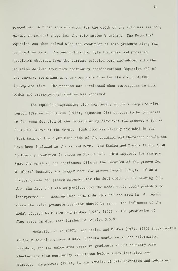
procedure. A first approximation for the width of the film was assumed,
giving an initial shape for the reformation boundary. The Reynolds'
equation was then solved with the condition of zero pressure along the
reformation line. The new values for film thickness and pressure
gradients obtained from the current solution were introduced into the
equation derived from flow continuity considerations (equation (4) of
the paper), resulting in a new approximation for the width of the
incomplete film. The process was terminated when convergence in film
width and pressure distribution was achieved.
The equation expressing flow continuity in the incomplete film
region (Etsion and Pinkus (1975), equation (2)) appears to be imprecise
in its consideration of the recirculating flow over the groove, which is
included in two of the terms. Such flow was already included in the
first term of the right hand side of the equation and therefore should not
have been included in the second term. The Etsion and Pinkus (1975) flow
continuity condition is shown on Figure 3.1. This implied, for example,
that the width of the continuous film at the location of the groove for
a Tshort' bearing, was bigger than the groove length U > L q). If as a
limiting case the groove extended for the full width of the bearing (L) ,
then the fact that Z>L as predicted by the model used, could probably be
interpreted as meaning that some side flow had occurred in a region
where the axial pressure gradient should be zero. The influence of the
model adopted by Etsion and Pinkus (1974, 1975) on the prediction of
flow rates is discussed further in Section 3.5.8.
McCallion et al C1971) and Etsion and Pinkus (1974, 1975) incorporated
in their solution scheme a zero pressure condition at the reformation, t 1 n res sure gradients at the boundary wereboundary, and the calculated pressure g
**. ^nndifinns before a new iteration was checked for flow continuity conditions oerorMQftn in his studies of film formation and lubricant started. Hargreaves Q981J, in

52
- a
1 / 2L / 2 r o
q dz = x
(q ) dz + x o
1/2
K h d z
where (q ) is the flow per unit width, x
Figure 3.1 The Etsion and Pinkus (1975) flow
continuity condition in the incomplete
film region (aQ £ ct £ a^)

53
flow rate in thrust bearings, adopted a different approach; the pressure
gradient boundary condition was incorporated into the equation to be
solved at the current reformation boundary location and a check for
constant cavitation pressure along the boundary was carried out after
the solution for the pressure had been obtained. The relocation of
the boundary was made at every mesh line by simple interpolation or
extrapolation between the point on the boundary and the node just inside
the boundary.
Ruddy (1979) carried out a numerical analysis of circumferentially
grooved bearings as part of a more extensive programme of work concerning
both static and a dynamic analyses of various fluid film journal bearing
types. Using the Reynolds boundary conditions at film rupture and the
condition of zero pressure at the film reformation, a cavitation region
was obtained by setting all negative nodal pressures in each iteration
cycle to zero. The calculated flow rates into and out of the bearing
were found to be different and this lack of flow continuity in the
axial direction was attributed to an incorrect reformation boundary
condition. The Jakobsson and Floberg (1957) reformation boundary
condition was then incorporated. The computer solution technique was
as follows. An initial estimate of the cavitation zone was obtained
putting all negative pressures equal to zero in each cycle. The
pressure gradient at a number of nodes on the current reformation
boundary was calculated and compared with the pressure gradient required
to satisfy continuity. This provided a criterion for moving the
reformation boundary to start the next iteration. After each iteration
the axial flow rates into and out of the bearing were calculated and
compared. The solution was taken to have converged when the two axial
flow rates had converged to within a given tolerance.

54
The programming complexities arising from film reformation
considerations, requiring the location of the reformation boundary and
the determination of pressure gradients at the interface, were
completely eliminated in a new approach to the problem of locating
cavities initially proposed by Elrod and Adams (1974) and later
refined by Elrod (1981), which was seen as an important step forward
in the analysis of liquid lubricated bearings. Elrod (1981) presented
a computational algorithm which allowed the automatic delimitation of
the cavitation region without explicit reference to boundary
conditions, and was valid for both steady and transient operating
conditions. A 'universal' differential equation was employed throughout
the whole lubricating region. This equation incorporated a 'cavitation
index' (g) which, by taking the value zero (in the cavitation region)
or unity (in the full film region), allowed the equation to change its
form. In the full film region the equation was elliptic and was
basically the Reynolds' equation. In the cavilation zone the equation
became parabol ic in form. Mass flow continuity was achieved in the
cavitation region as well as in the rupture and the reformation
boundaries, and the Reynolds' rupture boundary condition and the
Jakobsson and Floberg reformation boundary condition were automatically
imposed.
To test the algorithm, the analysis of various bearing types was
carried out by Elrod (1981). Good agreement was reported between the
predictions of these analyses and exact solutions or experimental data
provided by other workers.
Lebeck (1981) employed the Elrod cavilation algorithm in the
analysis of mechanical face seals and reported good correlation with
previous results and a significant decrease in computation time in

55
comparison with traditional techniques.
Finite difference approximations to the governing Reynolds'
equation have been widely used in the study of the performance of
hydrodynamic bearings. In recent years, however, finite element methods
have also enjoyed the interest of lubrication researchers. Finite
elementry may have an advantage over finite difference methods in the
facility with which curved boundaries and complicated boundary
conditions can be accommodated.
Milne (1974) presented a technique for calculating oil flow in
bearings based upon computation of a stream function using the finite
element method. The technique was applied to the case of a plane slider
bearing to which the effect of the shape of the elements on the
computation time and on the accuracy of the solutions was studied.
Hayashi and Taylor (1980) used a finite element approximation
technique and the Newton~Raphson iterative solution method in the
analysis of liquid film journal bearings. The predictions of the
analysis for the location of the rupture boundary and the bearing
performance were in good agreement with results obtained from a finite
difference analysis and exact analytical solutions. Tvw* advantages of
using the finite element approach were mentioned.
(i) the ability to locate precisely curved boundaries
(ii) the ability to apply with ease flow boundary conditions
Film reformation was not considered but it was pointed out that the same
approach would be equally successful for the more complex reformation
boundary conditions.
The apparent simplicty and ability to incorporate realistic
lubricant supply conditions exhibited by the Elrod cavitation algorithm

56
and the convincing results reported by Elrod (1981) and Lebeck (1981),
seemed to make the algorithm attractive to the purposes of the present
work.
The remainder of this chapter will be devoted to a discussion of
the technique developed for the analysis of finite width journal
bearings considering the lubricant supply conditions, which was based on
Elrod's algorithm. A careful study of the effect of influential
parameters on the computation time required for convergence of the
solution and on the accuracy of the predictions, will be described.
3.2 Elrod's Cavitation Algorithm
In oil film bearing analysis, the oil is usually assumed to be
incompressible. However, although mineral oils have low compressibility,
their density does increase with increasing pressure. The compressibility
is dependent on temperature and pressure, in general increasing with
increasing temperature and decreasing with increasing pressure.
3.2.1 The Bulk Modulus of the Lubricant
The inverse of the compressibility is called the 'bulk modulus .
Peeler and Green (1959) defined the mean bulk modulus of a fluid (B) as,
6 = vo V -V
o
(3.1)
where, (V) is the volume at the pressure (p)
(V ) is the volume at the reference pressure (PQ) »o
usually atmospheric
Galvin et al (1964) measured the percentage change in the volume
of various mineral oils that occurred with a known pressure variation
and at constant temperature (of 20° and 100°C). From their results the
bulk modulus of lubricating oils was found to be in the range 10? - 10
N/m2

57
3.2.2 Elrod's Variable (9)
Exploring the dependence of the lubricant density on pressure,
Elrod (1981) expressed the pressure in the full film region of the
bearing as
p = P c + e (6-1) (3.2)
where (p ) is the cavitation pressure and
0 = — , is the ratio of the lubricant densities at the pc
pressures (p) and (p ) respectively. In the full film
region, where p * p , 0 * 1.
In the cavitation region the pressure (pc) was assumed to be
constant and it was taken as zero in the present analysis. There was
thus no flow of lubricant in the axial direction in this region and the
Poiseuille component of the circumferential flow was zero. Due to
changes in film thickness, the lubricant film breaks down and does not
completely fill the clearance space. The Elrod variable (0), when
referring to the cavitation region, had a different meaning; it was
defined as the fraction of the bearing width occupied by the lubricant.
3.2.3 The Cavitation Index (g)
A cavitation index (g) was defined from a knowledge of (0) as
follows:
g = 0 where 0 < 1 (cavitation zone)
(3.3)
g = 1 where 0 * 1 (non cavitation zone)
It will be seen in the next section that the introduction of (g)
in the equations had the purpose of changing their form and thus making

58
them appropriate to the relevant film region.
3.2.4 The Cavitation Algorithm
Figure 3.2 represents the finite difference star and the
computational cell (of dimensions (Ax), (Ay) and (h)) used by Elrod.
assumed to be greater than or equal to zero.
The following algorithm was proposed by Elrod (1981) for the
convective (Couette) and pressure (Poiseuille) flow contributions to
the mass flow entering the cell in the x-direction (the subscripts refer
to points in the finite difference star).
(1) Convective mass flow per unit width of the bearing
When both nodes (-1,0) were in the full film region the film
thickness at the cell wall was averaged. Otherwise it was taken as
the film thickness at the upstream point (point —1)
(2) Pressure mass flow per unit width
which takes the usual form in the complete film region, is, zero in
the cavitation region and is interpolated at the rupture and
reformation interfaces.
The shaft surface speed (U^) and the bush surface speed (U-) were
(m ) x c
= Pc ( W2
g , g„+ — 7.— (h -h ) 2 o - l
(3.4)
(3.5)

59
3.3 The Final Finite Difference Equation
The total mass flow per unit width entering the cell in the
x-direction was given by the sum of expressions (3.4) and (3.5).
Similar expressions could be obtained for the mass flow per unit width
leaving the cell in the x-direction and for the mass flow in y-direction.
The finite difference equation having (0) as the dependent
variable was obtained from mass conservation considerations within the
cell. For steady state operating conditions the mass of lubricant in
the cell should not change. Thus,
(Ay) Am + (Ax) Am = 0 (3.6)J x y
where (Am ) and (Am ) are the net mass flows per unit width entering the x y
cell in the (x) and (y) directions.
The lubricant film was discretized by dividing the bearing area
into a number of small areas defined by perpendicular mesh lines in the
circumferential (x) and the axial (y) directions. Points in the grid
were identified by the subscripts (i,j) corresponding to the intersection
of the circumferential mesh line (i) with the axial mesh line (j).
Figure 3.3 shows the computaticmal cell, containing the grid point (i,j),
surrounded by unequally spaced mesh lines.
Equations (3.4) and (3.5) were applied to the four walls of the
cell and introduced into equation (3.6), thus allowing the derivation of
an equation for (0. •)• The bearing was assumed to be well aligned1 9 J
(film thickness not dependent on axial location).
The following dimensionless parameters were introduced at this
stage

60
Figure 3.2 The finite difference star and the
computational cell containing the
central point.
( i * 1 )
( U r ~
( i - 1 )
y
(tkX)jjj
U + 1 J )
0
(U )
Ax
A y
-1 (Ax)J
( W j
(A y l j _ ,
t j - 1 ) (J ) I i + 1 )
Figure 3.3 The computational cell surrounded by
unequally spaced mesh lines

61
(fl and
rad/s)
w h e r e ,
x =x
2irr y = b
h = e =
Q are the angular velocities of the shaft and the bush in
The following equation for (9. .) was derivedi > J
(tt/24) (Ax)(3(d/b) E 12 + (Ay/2)E1Q + (Ay/96x2Tr)6E11
(ir/24) (Ax)3(d/b) Eg + (Ay/2)Eg + (Ay/96x2ir)0E7
(3.7)
(Ax),
h? g. . „J
h? g. .. J \il.
(Ay)._1 (Ay)£
10 E 3 - E l
'11 E 2 + E4 + E 7
'12 V ’t ’ E9
+ 8 l . - j g i . i + l .. , h.. : * - - - 2— <»i+l - V1»J L »J
0^ , * gj.iri ^ i . j + l '0CAx)j

62
E 3 ' 9i,j-l 5j-l * Si,j-1 S j-1 +
8i,j-l (5. . I , >2 J J-1
(h.+h. J 3 g. . (0 . . - 1)F = 3 J-1 itJ-1 i»J-l
E , 5 i 8i-i..i (9i - i , r 1)5
h? g. , . (0 . , .-1)E = J 1+1»J 1+l.J
6 (Ay).
( A x ) . + ( A x ) , *Ax = 2
(Ay) . + (Ay) .A i - -----4 ---- —
3.4 The Analysis of Finite Width Journal Bearings With No Film
Reformation
The prime purpose of the present work was to undertake an analysis
of finite width journal bearings considering the lubricant supply
conditions in some detail. It was intended to treat the case of
lubricant supply via a single groove at the location of maximum film
thickness and, possibly, via one or two grooves at any location.
However, to gain confidence in the approach used and the predictions of
the analysis, the computer program was initially designed for non
reformation conditions only. The lubricant was assumed to be supplied
at amhient pressure via a full width line ’groove' at the maximum film
thickness. Most of the journal bearing performance predictions available
were obtained using this assumption and thus provided a good basis for
comparison of results.

63
3.4.1 The Finite Difference Mesh
A system of equations written in a finite difference form,
representing the application of equation (3.7) at each node, needed to
be solved. A finite difference mesh covering the bearing area was set
up by specifying the number of mesh lines parallel to the bearing axis
(M) and the number of circumferential mesh lines (N). The values taken
by the subscripts (i) and (j) in equation (3.7) were therefore in the
range
i : 1 to N
j : 1 to M
The axial mesh line (1) was coincident with the axial mesh line
(M) at the position of maximum film thickness. The circumferential lines
(1) and (N) were coincident with the bearing edges. The mesh lines in
both directions were equally spaced, the mesh size being dependent on the
specified values of (M) and (N).
3.4.2 Boundary Conditions
The boundary conditions required were the values of (0) at the
bearing edges and at the lubricant supply line. The pressure was taken
to be ambient at both locations. The lubricant was assumed to cavitate
at ambient pressure, Thus,
^amb ^In the full film region equation (3.2) applied. The boundary conditions
adopted were;
(a) At the lubricant supply line,
p = p = 0 and 0 - 1

64
(b) At the nodes on the bearing edges where a full width film
existed,
p = p = 0 and 0 = 1
(c) Within the cavitation region equation (3.2) was not applicable.
The values of (0) in this region were not related to the
cavitation pressure, they were obtained from the solution of the
system of equations (3.7). Due to the technique used which
required a knowledge of (0) at the nodes on the circumferential
mesh line (1) to calculate (0) at the nodes on the circumferential
mesh line (2), the following conditions were imposed.
for all nodes (2,j) and (N-l,j) in the cavitation region.
3 . 4 . 3 Method of Solution of the Finite Difference Equation
Approximations of the type represented by equation (3.7) resulted
in as many equations as grid points and the solution of a system of
simultaneous linear equations was required. The parameters involved were
(b/d), (e) (which determined (h)) and (B)* A Gauss-Seidel iterative
method was used. The following steps were involved in the procedure;
(1) Initially, the values of (0) and (g) at every node were set to
unity
(2) For any l
those where
iteration cycle (m>l) the value of (0) at every node (excluding
ere boundary conditions had been specified) was obtained from
6 On) * 9(m-1) + R f (0tcal) 6(m-l)(3.8)

65
where ®(-nr-i) ■'•s t ie v a lue calculated in the previous iteration
0 , is the value determined in the current iteration,(cal)
from equation (3.7)
is the relaxation factor
(3) After each iteration new values were given to (g) at every node,
according to the new values of (0) and equations (3.3)
(4) The iterative process was terminated once the solution had
converged. The convergence criterion was
s (m) 8(m-l) and (3.9)
(m) ®(m-l)^tolerance
(m-1)
at all nodes. The procedure returned to step (2) until
convergence was achieved.
3.4.4 Pressure Distribution in the Lubricant Film
Equation (3.2) which was applicable to the full film region
only, was written in dimensionless form as
P = B (0-1) (3.10)
where the dimensionless pressure (p) was given by
2“ _ Pp " n(«1+fi2)
(3.11)
The pressure distribution was determined from the distribution of (0)
according to
lf e i.:. > 1
.J

66
3.4.5 Load Capacity and Attitude Angle
The load capacity was determined by integration of the pressure
distribution around the bearing. For the coordinate system represented
in Figure 3.4, the components of the resultant film pressure force along
and perpendicular to the line of centres ((z) and (x) directions
respectively) were
2tt b/2
a -b/2
2 tt b/2
pr sin a dy da
(3.12)
pr cos a dy d:a
-b/2
where (a) is the circumferential variable measured from the position of
maximum film thickness in the direction of the shaft rotation.
Using equation (3.11) for the dimensionless pressure and taking
dy = b dy
and dot = 2ir dx
a dimensionless form of equation (3.12) was obtained
rl c lP = 2tt x
(p sin a) dy dx
o o
1 rl
(3.13)
P = -2 tt z
(p cos a) dy dx
o o
where the normal force components CPX ,PZ) were made dimensionless
according to

67
Figure 3.4 Coordinate system and normal force
components of the resultant pressure.

68
P =brri(^1+fi2> (3.14)
Simpson's rule was used to integrate each of the equations (3.13)
The dimensionless load capacity of the bearing and the attitude
angle were then determined from
and
W 4- 2 - 2 P + P x z
(3.15)
= tan-1 x
3.4.6 Lubricant Flow Rates
The computer program calculated the dimensionless flow rate from
the sides of the bearing (Q ), the flow rate into the cavitation region
(Q ) and the net flow issuing from the groove (Q ) when, at a later stage c
of the analysis, the lubricant inlet conditions were considered. The
approach adopted for the evaluation of the net flow issuing from the
groove is discussed in Section 3.5.3.
In the full film region, the flow in the circumferential
direction included both Couette and Poiseuille components. The flow in
the axial direction was pressure flow only.
The circumferential flow rate across a bearing section of
width (yx) was given by
.3 » (U,+U„)hdy (3.16)
ryl r h 3 3P + (V U2)hl
I2t\ a* 2
The axi al flow rate across a section of circumferential length
(x^) was determined from

In dimensionless form, equations (3.16) and (3.17) were written
as
Q.x (3.18)
o
Q.y (3.19)
o
where the flow rates were made dimensionless acording to
Q cb(Ux+U2)(3.20)
A knowledge of the pressure gradients at every relevant nodal point
was required before the numerical integration of equations (3.18) and
(3.19) could be carried out.
The Evaluation of Pressure Gradients
Figure 3.5 illustrates the method used to approximate the
pressure gradient (say in x—direction) at a node 0 . It was assumed
that in a small interval [0, 36], where (6) is the mesh size, the
pressure variation could be represented by a polynomial of degree three
the coefficients of which were calculated from a knowledge of the pressure
at the four nodes involved and denoted 0, 1, 2, 3 (see Figure 3.5).
The coefficient (B) was found to be given by
- - -2 ~3p (x) = A + Bx + Cx + Dx

70
p(x) = A + Bx * Cx^+ Dx^
Solve for (B) given that p =p0 at x= 0
P-S, x=S
p =p2 x = 28
p =p3 x=3$
Figure 3.5 Approximation used to calculate the
pressure gradient at the node 'O'.
71
-11 po - 18 Pl - 9 p 2 + 2 ^B ' 65-----------------
and the required pressure gradient at node 'O' was
9p
8xV.
= B (3.21)
x=0
The flow rates were determined using Simpson's rule to integrate
numerically equations (3.18) and (3.19).
3.4.7 The Computer Program Flow Chart
The program procedure was similar to that employed when film
reformation was considered. It will be discussed in Section 3.5.4.
3.4.8 A Study of the Convergence of the Solution
The parameters affecting the convergence of the iterative process
for given operating conditions (b/d, £), were the mesh size, the
tolerance adopted in the convergence criterion, the relaxation factor (R^)
and the bulk modulus parameter of the lubricant (3)•
The smaller the mesh size or the tolerance adopted, the larger
the number of iterative cycles required to achieve convergence and also
more accurate the solution obtained.
Elrod and Adams (1974) and Elrod (1981) have mentioned the
possibility of numerical instabilities for particular values of (3) and in
the former paper the use of 6 = 6.9 x 10? N/m2 was reported for reasons of
stability of the solution.
Elrod (1981) showed that, providing convergence had been achieved,
the value of (I) used had no significant effect on the bearing performance
predictions. A preliminary investigation on the influence of (Rf) and
(6) seemed to suggest that whatever the value of (6), convergence within
a minimum number of cycles was achieved for a value of (Rf) of about

72
unity. A more detailed study was carried out to investigate these
effects fully.
Influence of the Bulk Modulus Parameter
Solutions were obtained for a number of operating conditions
taking = 1, tolerance = 1 0 , M x N = 51 x 11 and for variable (8).
It was found that the optimum value of ((3) for a minimum number of cycles
for convergence was dependent on (b/d) and (e), and for a given (b/d)
the optimum value of (3) increased with increasing (e), as shown in
Figure 3.6. The following was also observed;
(a) The value of (8) used did not affect the performance predictions
except for very high values of (8)- For values of (8) corresponding
to 8^10 ^ it has been observed in a number of cases that convergence
was achieved, but to the wrong pressure distribution. This was
cured by using a smaller tolerance.
(b) Although the final pressure distribution was not affected by the
value of (B) used, the values of (0) in the full film region were
obviously affected. For values of (8) corresponding to B <10 , (0)
was much greater than unity in the full film region due to the assumed
relatively high compressibility of the lubricant.
(c) In the cavitation zone (0) was almost unaffected by changes in (8).
As an example, for typical operating conditions,
C /d = 0.002, ft, - 125 rad/s, fl- = 0, n * 0.02 Pa.s and d *
B = 5 x 10⁷ N/m , the value of (B) would be 80.
The influence of the bulk modulus parameter on the convergence of
the solution will be discussed further in Section 3.5.6.

Bulk
Modu
lus
Para
meter
73
Figure 3.6 Values of (8) for convergence within a
minimum number of cycles.
M x N = 51 x 11, R f = 1

74
Optimum Relaxation Factor
The influence of the relaxation factor on the number of cycles
for convergence is shown in Figure 3.7 where three different operating
conditions are considered. The values of (B) used were obtained from
the previous study to ensure rapid convergence.
A decrease in the number of cycles was initially observed as
(R^) increased from a value less than unity. Convergence within a
minimum number of cycles was in general achieved for (R^) in the range
(1—1.05). A further increase in the value of (R^) resulted in either the
number of cycles for convergence to increase very sharply or, more
commonly, the program to be interrupted due to 'overflow'.
Case 2 (Figure 3.7) was chosen for a closer look into the
iterative process for values of (R^) in the neigh bourhood of its optimum
value. It was observed that when (R^) varied from 1 to 1.04 the number
of cycles decreased further to 72 and for R f = 1.047 to 1.04718 the
number of cycles was 71. Then, suddenly at Rf « 1.04719 'overflow'
occurred. When the values of (0) at various nodes and for successive
iterative cycles were printed out, it was found that with a given number
of cycles performed some of the nodes had already converged. With the
continuation of the iterative process the values 0(m_1} and 0(m) those nodes, stayed for a while within the tolerance varying in an
oscillatory fashion. However, after a number of cycles, variable frc
node to node, the value 0 (m) started moving away from 0 (m_ 1}. For a
given value of 0(m_ 1} the resulting 0(m) became bigger and bigger as the
iteration progressed and 'overflow' eventually occurred.
The value R f - 1 was therefore adopted. This consideration of
optimum relaxation factor and instability will be discussed further in
Section 3.5.7.
at
:om

Numb
er of
Cycle
s
75
120
110
100
90
80
70
b/d a nA O.U 0.5 50 0.5 0.7 28+ 0.6 0.8 95
60
±
0.9 1.0 1.1Relaxation Factor, R*
Influence of the relaxation factor
on the number of cycles for
convergence
Figure 3.7
M x N = 51 x 11, tolerance = 10-5
76
Optimum Tolerance
The influence of the tolerance on the number of cycles for
convergence and on the accuracy of the solution, is shown in Figure
3.8. The ratio of the values of load capacity (W), attitude angle (if))
and side flow (Q ), to the values of the same quantities for the
_ Q _ _ _ \
tolerance 10 (e.g. W r = w/wtol=10-8 are <iuoted-
The tolerance 10 was considered to represent a satisfactory
compromise between accuracy and number of cycles required for convergence.
It was therefore adopted.
3.4.9 Comparison of the Predictions of the Current Analysis with
Published Results
The results of the current analysis were checked against the
predictions of ESDU Item No. 66023 (1966), Ashton (1973) and King (1975)
for load capacity and flow rates. Figures 3.9 and 3.10 show very good
correlation for b/d = 0 . 5 . Equally good was the correlation observed
for b/d = 0.75 and b/d = 1. The dimensionless flow rates of ESDU Item
No. 66023 (1966) corresponding to the inlet flow (Q.) and to the side
flow (Q ) were (Qg) and (C^) respectively (apart from a constant).
3.5 The Analysis of Finite Width Journal Bearings Considering Film
Reformation
The analysis discussed in Section 3.4 was extended to include a
detailed study of the lubricant supply/reformation conditions. Only the
case of a single axial groove (or single 'square* hole) at the position
of maximum film thickness was studied.
Three more parameters were introduced to enable consideration
of the new situation of lubricant heing supplied to the bearing via a groov

Numb
er of
Cycle
s
77
Figure 3.8 Influence of the tolerance on the number
of cycles for convergence and on the
accuracy of the solution,
b/d = 0.5, e = 0.7, B = 28
M x N = 51 x 11, Rf = 1

Dime
nsion
less
Load
Capa
city,
78
Figure 3.9 Comparison of theoretical results for
dimensionless load capacity without
considering reformation, b/d = 0.5

79
x
+ King (1975)
.________________ L_______________ I---------------- 1—Q2 0.4 0.6 0.3
Eccentricity Ratio, &Figure 3.10 Comparison of theoretical results for
dimensionless flow rate without
considering reformation, b/d = 0.5

80
at a supply pressure greater than anbient. The groove geometry was
accounted for by the introduction of the parameters (a/b) and (w/d)
related to the axial and the circumferential dimensions of the groove.
The lubricant supply pressure was introduced by means of the
dimensionless supply pressure (p^).
3.5 .I The Variable Finite Difference Mesh
The axis of the journal was assumed to be parallel to the
bearing axis. The distribution of pressures was symmetric about the
bearing centre line and it was therefore sufficient to solve equations
(3.7) for half the bearing area only.
The accuracy of the location of the reformation boundary was
found to affect the calculated flow rates, a matter which will be
discussed in Section 3.5.5.
A mesh of variable size was used to cope with the presence of
the groove and the degree of accuracy required in the location of the
reformation boundary. Only (M) and (H), the number of mesh lines in the
(x) and the (y) directions respectively, needed to be specified. A
variable mesh covering half the bearing area was set up automatically
by the computer program with the following features;
(a) One mesh line was always coincident with each groove edge
(b) The number of grid intervals over the groove was dependent
on the groove size
(c) There was always at least three equally spaced intervals around
the groove edges and near the bearing edge, such that equation
(3.21) could be used to calculate pressure gradients
, . - -j intervals over the film reformation region in(d) The number of grid intervene
the circumferential direction was dependent on (£f) and (a/b).

81
Figure 3.11 shows two automatically generated grids for two
different lubricant inlet conditions. Details on the automatic
generation of the variable mesh are given in Appendix A.
3.5.2. Boundary Conditions at the Groove
The boundary conditions at the bearing edge were the same as
those discussed in Section 3.4.2. At the groove the pressure was
assumed to be constant and equal to the lubricant supply pressure. The
values of (0) at all nodes over the groove were kept constant throughout
the solution procedure at a value given by equation (3.10).
A simple calculation of the pressure drop associated with the
acceleration of the oil from the groove into the bearing showed that it
was of about 0.01 bar (1 kN/m2) for a tangential speed of the shaft
of 3 m/s, and of about 0.25 bar (25 kN/m2 ) for a tangential shaft speed
of 15 m/ s .
3.5.3 Evaluation of the Flow of Lubricant Issuing From the Groove
The flow rate of lubricant supplied to the bearing through the
groove should be equal to the flow rate from the bearing sides. These
flow rates were obtained from different calculations and the correlation .
between them was used to assess the accuracy of the solution.
The evaluation of flow rates has been discussed in general terms
in Section 3.4.6. The approach adopted for the evaluation of the
dimensionless flow rate issuing from the groove (Qgr> is sketched in
Figure 3.12. Three situations were considered covering the full range
of supply pressures.

82
(a) P, = 0 j a /b = 0.6, w/d=0.15
(b) p =0.25, a/b = 0.4, w/d = 0.2
Figure 3.11 Two automatically generated grids showing the
dependence of mesh size on groove geometry
and supply pressure
( M x N = 91 x 19)

83
(a) p = 0 ( Q 3 = 0 , Q ^ = - Q ^ ( a / b ) )
(b) p> 0 (small) (Q j= - Qc (a/b))
( c ) p » 0 (& - (2 * - (Q a /b )) f 1 1 c
Figure 3.12 A sketch of the partial flows considered
in the calculation of the flow of lubricant
issuing from the groove
< V ‘ 51 * ^ 2 * V
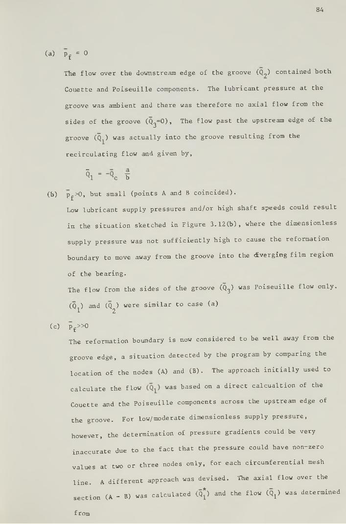
84
(a) p f = 0
The flow over the downstream edge of the groove (Q^) contained both
Couette and Poiseuille components. The lubricant pressure at the
groove was ambient and there was therefore no axial flow from the
sides of the groove (Q3= 0 ) , The flow past the upstream edge of the
groove (Q ) was actually into the groove resulting from the
recirculating flow and given by,
\ = ¥
(b) p f>0, but small (points A and B coincided).
Low lubricant supply pressures and/or high shaft speeds could result
in the situation sketched in Figure 3.12(b), where the dimensionless
supply pressure was not sufficiently high to cause the reformation
boundary to move away from the groove into the diverging film region
of the bearing.
The flow from the sides of the groove (Q3) was Poiseuille flow only.
(Q ) and (Q ) were similar to case (a)1 2(c) pf» 0
The reformation boundary is now considered to be well away from the
groove edge, a situation detected by the program by comparing the
location of the nodes (A) and (B). The approach initially used to
calculate the flow was based on a direct calcualtion of the
Couette and the Poiseuille components across the upstream edge of
the groove. For low/moderate dimensionless supply pressure,
however, the determination of pressure gradients could be very
inaccurate due to the fact that the pressure could have non-zero
values at two or three nodes only, for each circumferential mesh
line. A different approach was devised. The axial flow over the
section (A - B) was calculated CQ*) and the flow C Q ^ was determined
from

85
Q x - Q* - (Qc £>
This expression ensured a consistent variation of (Qi) with (p^). If
(A) and (B) were coincident = 0 and (Q^) was reduced to case (b).
As the dimensionless supply pressure increased, (Q-) increased and there
was a value of (p_) for which (Q, = Q . As a result the net flow t 1 c b
past the upstream edge of the groove would be zero. A further increase
in (p~) resulted in a positive value of (Q^)» indicating that there was
a net flow out of the groove from its upstream edge.
The total net dimensionless flow issuing from the groove was
given by
V • \ \ % (3.22)
3.5.4 The Computer Program
A computer program incorporating the previously discussed details
was written in Fortran IV, the flow chart for which is shown in Figure
3.13. Double precision was employed throughout the program to minimize
the effect of truncation errors.
The solution of a number of cases of different operating
conditions was allowed for during one run of the program. The number of
cases was read in as (NCASE) and (IC) was the counter for the number of
cases which had already converged. Two parameters were controlled during
the execution of the program.
(a) The number of cycles performed during the solution of each case
which was held in (NCYCLE) . The program was stopped if convergence
had not been achieved in a number of cycles smaller than a maximum
preset value (NCYMAX)
(b) The total cpu time used. The program was stopped when the total

86
Figure 3.13 Computer program flow chart

87
cpu time (CPU) exceeded the preset maximum cpu time (CPULIM).
The solutions already obtained were kept in an output file,
including a record of the cpu time used in each solution .
The program was implemented on the Amdahl 470 Computer System at the
University of Leeds.
The program coding and sample input and output data are listed
in Appendix B.
3.5.5 Mesh Size and the Accuracy of the Solution
In the first instance, apart from the region over the groove,
the mesh lines parallel to the (y) axis were equally spaced. When a
grid of (51x11) nodal points over half the bearing area was used,
significant discrepancies were observed between the calculated values
of (Q ) and (Q ). To invesitgate the cause of such discrepancies the gr s
simpler case of p^ = 0 was considered.
For flow continuity to be satisfied with p^ = 0 the circumferential
flow rate of lubricant over the bearing section corresponding to the
intersection of the calculated reformation boundary with the bearing edges
(Q , in Figure 3.12(a)), should be equal to the flow over the bearing
section at the downstream edge of the groove. That is, for flow
continuity in the reformation region the following equation should be
satisfied
Q r - Q2 + Q c < * * f > <3 '23>
The discrepancy observed between the left and the right hand sides of
equation (3.23) was, in general, in the range 5-8%. At low (a/b),
however, this discrepancy was as high as 12%.
88
Considerable time and effort was invested in the investigation
of this discrepancy. The calculated pressure gradients and the numerical
integrations were checked against hand calculations for a pre-fixed
pressure distribution. They were found to be correct. When a balance
of flows at nodes on the reformation boundary were worked out, it was
found that flow continuity was not satisfied. This could be due partly
to the approximations involved in the cavitation algorithm or, more
likely, to inaccurate location of the reformation boundary. If, for
example, the reformation boundary intersected the bearing edge at 40 from
the groove location, the maximum error in the location of that point of
intersection would be one circumferential mesh interval (about 7° for
M = 51). The error introduced in the dimensionless film thickness (h)
would be of about 4.5% at e = 0 .8, and because the pressure flow is a
-3function of h , the error introduced m the determination of flow rates
could be as m u c h as 13%.
The number of mesh lines was increased in both circumferential and
axial directions. The general results could be summarized as follows:
(1) An increase in the number of node points resulted in a decrease in
the discrepancy observed between both sides of equation (3.23), but
also an increase in the computer cpu time required.
(2) The values that changed significantly were (Q^) and (Qg) only, (Q ),
(Qt and (W) were not much affected by a change in mesh size. This
reinforced the idea that the discrepancies observed were mainly due
to inaccuracy in the location of the reformation boundary.
(3) For the same total number of nodes, the cpu time was higher for
higher values of CN). For a grid of (M — 125, N •<* 25) or higher,
it simply was not possihle to get a solution in an acceptable cpu time.

89
(4) At M = 91, N = 19 the maximum discrepancy observed was 7.5%
corresponding to the case to which a 12% discrepancy had been
observed at M = 51, N = 11. The cpu times used were in general
acceptable.
A mesh with a total number of grid points (91 x 19) was therefore
adopted.
A much more acceptable discrepancy in the flow continuity
condition (3.23) was observed when a variable mesh was used, as discussed
in Section 3.5.1. The mesh intervals in the circumferential direction
over the reformation region upstream and downstream of the groove
corresponded to about 2 .
A matrix of solutions obtained with a variable mesh of (91x19)
nodes, for variable (b/d), (e), (a/b) and(p^)> showed that the discrepancy
between (Q ) and (Q ) was now usually less than 5% (often between 3% gr s
and 5%). At p~=0 and a/b ( 0.5 this figure could rise to 6.5%. A
significant increase in cpu time with respect to the case of an even
mesh with the same number of nodes, was also observed.
Bearing in mind the purpose of the computer solutions obtained,
a variable mesh of (91x19) nodes seemed to be an acceptable compromise
between accuracy and computation time.
3.5.6 Computation Time for a Single Solution
The influence of relaxation factor, tolerance and bulk mudulus
parameter on the convergence of the Gauss-Seidel iteration has been
discussed in Section 3.4.8 for the case where film reformation was not
considered.
In the present analysis where the lubricant supply conditions were
considered and a variable mesh with an increased total number of nodes

90
was adopted, a relaxation factor of unity usually gave minimum cpu
time at given values of (8) and tolerance. Here again the values unity
for relaxation factor and 10 for tolerance were adopted. When the
values of (8) recommended for non-reformation conditions were used in
the present analysis many situations of 'overflow' were encountered.
A detailed study of the influence of (8) on the convergence of the solution
showed that now convergence was, in general, only achieved with values
of (8) equal to or less than 0.1. Figure 3.14 shows the effect of the
value of (8) on the number of cycles for convergence for the operating
conditions indicated in the figure.
A minimum number of cycles was normally obtained with values of
(8) in the range (0.01-0.03). The cpu time required for a single solution
using values of (8) within that range was usually of 250 to 350 cpu
seconds and seemed to be affected more significantly by the values of
(a/b) and (p^). Those figures could, however, be doubled in some cases
at low (a/b) and ambient supply pressure.
The value of (8) adopted did not affect significantly the
solution; performance predictions at given operating conditions obtained
using different values of (8) were normally equal to the third decimal
place.
3.5.7 An Attempt to Reduce the Computation Time
An attempt was made to reduce the cpu time required for convergence
by using over-relaxation in the full film region only. Elrod (1981)
pointed out that equations of the type (3.7) were elliptic in the full
film region and parabolic in the cavitation region, and Smith (1971)
showed that the Gauss-Seidel over-relaxation iterative method was the
most efficient for the solution of elliptic partial differential equations.

Numb
er of
Cycle
s
91
2000 7
1.0
1500
1000
700
t 1 ± i. JL ±0.003 0.005 0.01 0.03 0.05 0.1
Bulk Modulus Parameter. H
Figure 3.14 Influence of the value of (B) on the
number of cycles for convergence
MxN = 91 x 19, variable mesh size
b/d = 0.5, e = 0.7
a/b = 0 .8, w/d = 0.2R = 1, tolerance = 10
-5

92
Over-relaxation was used with the equations corresponding to nodes
in a full film region initially guessed using the same approach as used
before to define the variable mesh (Section 3.5.1). For the end of the
continuous film region a conservative location of the rupture boundary
at a = 190 was assumed. The over-relaxation factor used was either
entered as data or, alternatively, an optimum over-relaxation factor wasI
calculated by the program according to the method proposed by Randall
(1968). For grid points outside the guessed full film region (R^) was
unity.
Very good results were obtained for a number of cases studied,
with reductions in cpu time of the order of 50%. Unfortunately, cases
of 'overflow' and consequent interruption of the solution were also
encountered without it being possible to make any improvement on the
situation. The use of two different values of (R^) was therefore
abandoned.
3.5.8 Comparison of the Predictions of the Analysis With Published
Results
Published results of a direct analysis of finite width journal
bearings considering the lubricant inlet conditions were scarce and usually
only applicable to situations of lubricant supplied at ambient pressure.
McCallion et al (1971) considered both the groove geometry and
the lubricant supply pressure but only the case of a groove located at
the load line. The similarity in the shape of the rupture and reformation
boundaries compared with the predictions of the present analysis is,
however, worth noting.
Etsion and Pinkus (1975) presented results of the analysis of
finite width journal bearings with incomplete films for a range of values

93
of (b/d), (e) and (a/b), the lub ricant supply pressure being ambient.
Very poor agreement was observed when their results were compared with
those of the present analysis. The most significant discrepancies were
observed for side flow and for the location of the reformation boundary,
at low values of (a/b). The comparative results are shown in Figures
3.15 and 3.16.
The discrepancies observed could be partly explained by the
continuity condition used by Etsion and Pinkus in the film reformation
region (equation (2) of their paper), and already discussed in Section
3.1. Such a condition would be equivalent to an increase in the flow rate
past the downstream edge of the groove, by a fraction of the cavitation
flow corresponding to the groove length. This increased inlet flow was
responsible for the higher values of (Q ) and the lower values of (a^)
observed. Also the increase on the observed discrepancies for decreasing
eccentricity ratio, was seen as the effect of the increasing significance
of the recirculating flow.
Non-reformation conditions could be simulated in the present
analysis by taking p^ = 0, a/b = 0.999 and w/d = 0.001. When the results
for load capacity and flow rates, for b/d = 0 . 5 , were compared with those
obtained from the non—reformation analysis discussed in Section 3.4, the
correlation observed was within 0.5%.
3. 6 Conclusions
(1) Prior to the presentation of a cavitation algorithm by Elrod (1981),
a refinement of previous work by Elrod and Adams (1974), the
delineation of the region of the bearing where the film cavitates was
dependent on an explicit reference to some boundary conditions.
Normally, film reformation has not been considered; the lubricant
has been assumed to be supplied at ambient pressure yia a line

Dimen
sionle
ss
Flow
Rate,
94
Figure 3.15 A comparison of the predictions of dimensionless
side flow rate from the present analysis with
those presented by Etsion and Pinkus (1975).
b/d = 0.5, a/b = 0.5, p, = 0
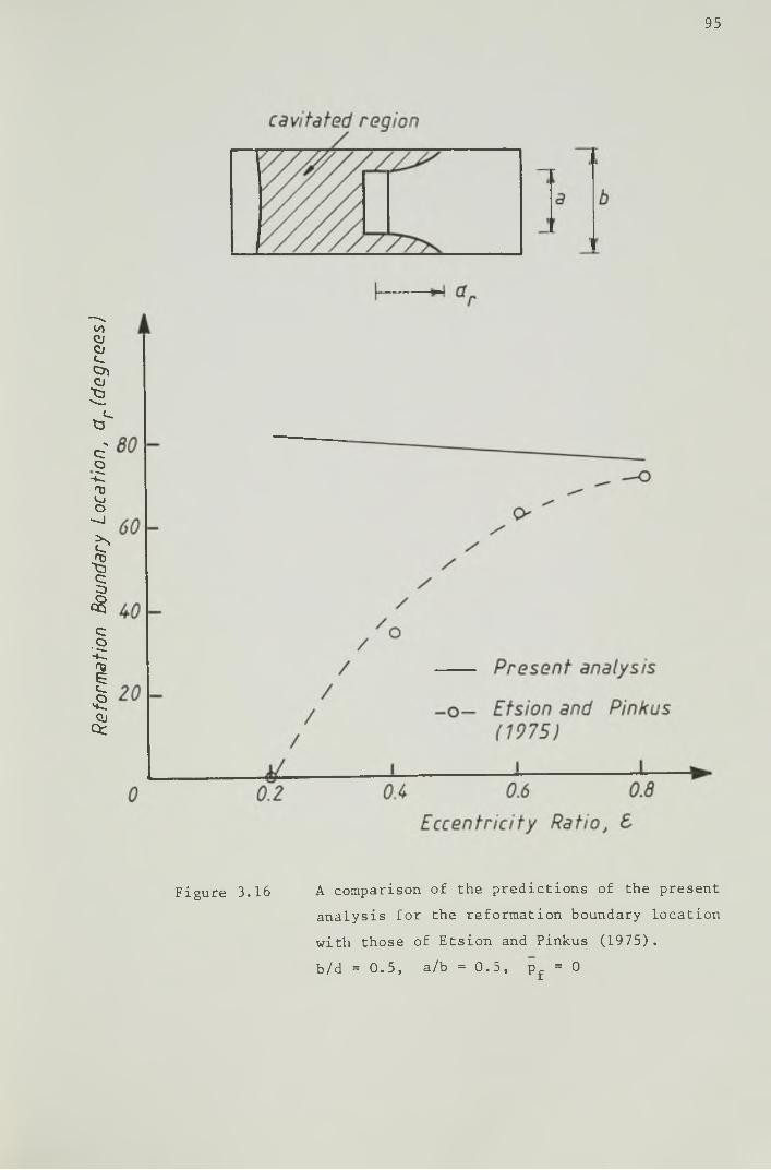
Refor
matio
n Bo
undary
Lo
catio
n, dr
(degre
es)
95
Figure 3.16 A comparison of the predictions of the present
analysis for the reformation boundary location
with those of Etsion and Pinkus (1975).
b/d = 0.5, a/b = 0.5, p f = 0

96
groove located at the maximum film thickness. A condition based
on flow continuity has normally been used to locate the rupture
boundary. Such an analysis has been largely adopted for two main
reasons:
(i) The difficulties arising from the inclusion of a reformation
boundary condition in the numerical analysis
(ii) The fact that the load capacity would not be significantly
influenced by the lubricant inlet conditions.
The development of high speed, large storage digital computers
made possible the consideration of both the rupture and the
reformation boundary conditions. McCallion et al (1971) and Etsion
and Pinkus (1975), among others, obtained solutions for finite
width journal bearings considering the film inlet conditions.
Elrod (1981) proposed a cavitation algorithm which was able to
deal with the cavitation region without the explicit formulation
of its boundary conditions. Flow continuity was achieved within
the cavitation region and across the boundaries. Very satisfactory
results of analyses incorporating the Elrod cavitation algorithm
were reported by Elrod (1981) and Lebeck (1981).
(2) A technique was developed for the analysis of finite width journal
bearings based on Elrod's algorithm. A system of simultaneous
equations in finite difference form derived from the application of
the algorithm and involving the normalized bearing parameters, was
solved over the bearing area using a Gauss-Seidel iterative method.
The case of non-reformation was first considered. A computer
program for determining the bearing performance under non
reformation conditions was written. A study of the parameters

97
affecting the convergence of the Gauss-Seidel iteration was
carried out, its conclusions being summarized as follows:
(a) There existed an optimum value for the bulk modulus parameter
(3) for quickest convergence which was dependent on (b/d) and
(e). Although affecting the number of cycles for convergence,
the value of (3) used did not affect significantly the bearing
performance predictions.
(b) A number of tests carried out using the optimum values of (3)
suggested that the optimum value for the relaxation factor
(Rf) would be about unity. 'Overflow' caused the program
operation to be interrupted in most of the cases to which R >1.
(c) The tolerance adopted as a compromise between accuracy of the
• , n -5 solution and number of cycles required was 10
The predictions of this analysis showed very good correlation with
published results.
(3) The analysis was extended to include the lubricant inlet conditions
for a single groove at the maximum film thickness. For reasons of
accuracy of the solution, a finer mesh (of about 2 intervals) was
used over the film reformation region. The flow of lubricant
issuing from the groove was calculated directly and the discrepancy
between this and the calculated side flow, was used as a measure of
the accuracy of the solution. For a grid of (91x19) nodes the
discrepancies observed were, m general, within the range 3 5%.
At p f = 0 and a/h £ 0.5 this discrepancy could, however, go up to
a-maximum of 6.5%. This was mainly attributable to the inaccurate
location of the reformation boundary.

98
A value of (R_) of unity and values of (B) within the range
(0.01-0.03) resulted, in general, in a minimum number of cycles
for convergence of the solution.
Published results of a direct analysis considering the groove
geometry and the lubricant supply pressure were not available.
Etsion and Pinkus (1975) presented solutions for the lubricant
supplied at ambient pressure. Correlation between the predictions
of the present analysis and those of Etsion and Pinkus (1975) was
not good. This was attributed mainly to their formulation of the
flow continuity condition in the film reformation region.
When conditions of non reformation were simulated by
taking p = 0, a/b = 0.999 and w/d = 0 .001, the results given by
the program were within 0.5% of the predictions of the analysis
that considered no reformation.
(4) Only the case of a single groove at the maximum film thickness has
been considered. It would not be difficult to extend the analysis
to the case of one axial groove at any location or indeed to a
consideration of two axial grooves. An iteration would then be
required to determine the correct attitude angle, and the cpu time
would be greatly increased. Thus, every effort to speed up the
convergence of the Gauss-Seidel iteration would be worthwhile.

99
CHAPTER 4
A COMPARISON OF RESULTS FROM THE PRESENT
ANALYSIS WITH THE PREDICTIONS OF ESDU
ITEM No. 66023 (1966) AND THE DEVELOPMENT OF
DATA CHARTS
4.1 Introduction
Most of the journal bearing design procedures available have been
based on numerical solutions of the Reynolds' equation which have in
corporated the assumption of lubricant supplied at ambient pressure via
a line 'groove' at the location of maximum film thickness. With real
lubricant inlet conditions film reformation would be unlikely to occur at
the line of maximum film thickness and, therefore, such an assumption
will lead to inaccurate predictions of the flow of lubricant in the
bearing (Cole and Hughes (1956), McCallion et al (1971), Etsion and
Pinkus (1974)). The influence of the lubricant flow rate upon bearing
performance as a whole has already been stressed in Chapter 1.
A commonly used procedure for the design of steadily loaded,
liquid film, hydrodynamic journal bearings, is the one described in ESDU
Item No. 66023 (1966) which has been briefly discussed in Section 2.2.
This procedure relied very heavily upon the use of design charts based
on data obtained from numerical solutions of the Reynolds equation in
which the lubricant inlet conditions were not fully considered .

100
One objective of the journal bearing analysis undertaken was to
carry out an investigation of the correlation of the bearing performance
predictions (flow rate in particular) of ESDU Item No. 66023 (1966),
with the predictions of a more accurate analysis in which film reforma
tion was considered. For this purpose, computer solutions were obtained
for all combinations of the values of the parameters shown in Table 4.1.
Additional solutions have been computed for the development of data charts.
Parameter Values
b/d 0.5, 0.75, 1.0
e 0.2, 0.4, 0 .6 , 0.8
a/b 0.5, 0.8, 1.0 (0.999)
w /d 0.2
Pf 0.0, 0.1, 0.25, 0.5, 1.0
Table 4.1 Values of the Parameters Considered
The maximum value of dimensionless supply pressure considered (pf=1.0)
corresponded to a bearing with a clearance ratio of 0.002 operating at a
journal speed of 500 r.p.m. (8.33 Hz) with a lubricant supplied at
? . / 2 250 kN/m and an effective viscosity of 0.019 N.s/m .
The performance predictions computed included:
(i)The dimensionless pressure distribution in the lubricant
(ii)The dimensionless load carrying capacity (W)
(iii) The attitude angle (<|>)
(iv)The dimensionless flow rate of lubricant issuing from the
groove (Q )•

101
(v) The dimensionless flow rate out from the bearing sides (Qg)
(vi) The dimensionless flow rate into the cavitation region (Q£)
(vii) The location of the reformation and the rupture boundaries.
The performance predictions (i) to (vi) were printed out
(see Appendix B) and the locations of the rupture and the reformation
boundaries were shown in a diagram of the 'developed' bearing area.
Figure 4.1 shows two of these diagrams for two different operating
conditions.
In this chapter, a study of the correlation between results from
the analysis undertaken and the predictions of ESDU Item No. 66023 (1966)
will be described and the development of data charts based on computer
solutions will be discussed.
4.2 A Comparison of the Reisults for Load Capacity and Attitude Angle
Results for dimensionless load capacity and attitude angle from
the present analysis were compared with the predictions of ESDU Item
No. 66023 (1966) for all combinations of the values of the parameters
shown in Table 4.1. The correlation observed could be sunmarized as
follows:
(a) For non-reformation conditions (p^ =0 and a/b=l) the correlation
observed for both (W) and (40 was good at all values of (b/d) and
(e) considered.
(b) For realistic lubricant inlet conditions the degree of correlation
was dependent on the values of the operating parameters. Figures
4.2 and 4.3 show the comparative results for dimensionless load
capacity and attitude angle for fixed b/d=0.5, a/b=0.8 and w/d=0.2 The discrepancies observed were more significant at low values of

102
SHAFT ROTATION FROH LEFT TO RIGHT
NORNALIZED SUPPLY PRESSURE * .000
b/d = .500 ECC = .600
a/b = .500 w/d = .200
CAVITATION REGION FULL FILd REGIONEDGE 192.2 DEG EDGE 310.5 DEGNOSE 196.7 DEG NOSE 331.5 DEG
180 nAX.SAP 180
SHAFT ROTATION FROM LEFT TO RIGHT
NORMALIZED SUPPLY PRESSURE = .500
b/d = .500 ECC = .600
a/b = .800 w/d = .200
Figure 4.1 The location of the reformation and the rupture
boundaries for two different sets of operating
parameters.
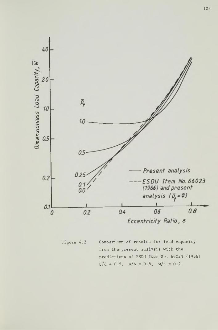
Dimen
sionle
ss
Load
Capa
city,
W
103
Figure 4 .2 Comparison of results for load capacity
from the present analysis with the
predictions of ESDU Item No. 66023 (1966)
b /d = 0 . 5 , a/b = 0 .8 , w/d = 0 . 2

104
Figure 4 .3 Comparison of results for attitude angle
from the present analysis with the
predictions of ESDU Item No. 66023 (1966)
b/d = 0 .5 , a/b = 0 .8 , w/d = 0 .2
105
(e) , increasing for increasing values of (p^)» This was a
consequence of the hydrostatic pressures in the groove region,
the significance of which, in comparison with the hydrodynamic
pressures developed in the film, was dependent on the lubricant
supply pressure and the size of the groove.
This pattern was unchanged at higher values of (b /d ) , the
discrepancies being, however, slightly smaller as (b/d) increased.
(c) Figure 4 .4 shows the effect of groove length on the dimensionless
load capacity at ambient supply pressure. The discrepancies here
were more significant at low values of ( e ) , increasing for
decreasing values of (a /b ) . Severe 'starved inlet conditions
( " f=0 , a/b < 0 .5) can be seen to affect significantly the load
carrying capacity of the bearing at low values of the eccentricity
ratio (e < 0 .6) .
At finite lubricant supply pressures and low values of (e) the
computer solutions for load capacity were greater than the
predictions of ESDU Item No. 66023 (1966) (see Figure 4 .2 ) .
In conclusion it can be said that;
(i) The accuracy of the predictions of dimensionless load carrying
capacity from ESDU Item No. 66023 (1966) at ambient supply pressure
and with a/b S 0 .5 , is good (with a maximum discrepancy of 9%) for
all values of (e) and (b/d) considered. At higher values of (pf)
the accuracy of the predictions was dependent on ( Pf) and ( e ) . In
general, for a given eccentricity ratio, the degree of accuracy
decreased with increasing values of (pf) , the discrepancies being
more significant at low values of ( e ) . At e > 0 .3 and pf * 0 .25 ,

Dimen
sionle
ss Loa
d Ca
pacit
y,
106
Figure 4 .4 Comparison of results for load capacity
from the present analysis with the
predictions of ESDU Item No. 66023 (1966)
b /d = 0 .5 , w/d = 0 .2 , pf = 0

107
a practical maximum value of dimensionless supply pressure, the
maximum discrepancy observed was about 10%.
(i i ) The predictions for atttitude angle of ESDU Item No. 66023
(1966) at p =0 and a/b ^ 0 . 8 , were in good agreement with the
predictions of the present analysis (with a maximum discrepancy
of 4 ) , for all values of (b/&) and (e) considered. At finite
values of dimensionless supply pressure significant discrepancies
can occur between the predictions of the two procedures. These
discrepancies increased with increasing values of (p^) and
decreased with increasing values of ( e ) . However, for practical
values of eccentricity ratio and dimensionless supply pressure
(e £ 0.6 and p . < 0 .25) the discrepancies observed were not
significant ( 8° at the maximum).
At a limiting value of eccentricity ratio equal to zero there will
be no hydrodynamic pressure generated. Hence, the load carrying
capacity of the bearing will be a consequence of the hydrostatic
pressure in the groove region alone, resulting in an attitude
angle of about 180 .
4 .3 Comparison of Results for Side Flow
In ESDU Item No. 66023 (1966) the lubricant flow rate in the
bearing was determined as the sum of a ’ zero supply pressure' flow (Qv)
with a 'zero speed' flow (Qp) » a method proposed by McKee (1952). (Qv)
was defined as the lubricant flow rate induced into the clearance space
by the rotation of the journal. It was actually side leakage but
incorporated a correction factor accounting for the length of the groove.
The flow (Q ) was defined as the flow rate of lubricant forced
through the groove, into the bearing, by the supply pressure and was

108
determined on the assumption of a stationary journal.
At zero supply pressure (Q ) became zero and the side flow rate,P
according to ESDU Item No. 66023 (1966 ), was reduced to (Q ) . Figure 4 .5
shows a comparison of results for dimensionless side flow from the present
analysis with the predictions of ESDU Item No. 66023 (1966 ), at b /d=0.5
and p^=0. The correlation was good at a/b=l and a /b=0 .8 . As (a/b)
decreased the discrepancies increased, being about 12% at a /b=0 .3 and
£=0.8. The same trend was observed for the other values of (b/d)
considered, the discrepancies showing, however, a slight tendency to
increase with increasing values of (b /d ) for given values of (a/b) and ( e ) .
At finite lubricant supply pressures the side flow predictions
from ESDU Item No. 66023 (1966) were given by (Q +Q ) . The presence of
the viscosity of the lubricant in the formula giving the flow rate (Q ) ,
made a comparison of flows in dimensionless terms difficult , thus preventing
a comparative study of results for a wide range of operating conditions.
The option left was to compare the dimensional side flow rates at different
operating conditions. A bearing with the following specifications was
considered:
d = 5 0 mm
b /d = 0 . 5
C ,/d = 0.0015 a
Journal speed = 800 r.p .m . (13 .33 Hz)
Single groove at the maximum film thickness
a/b = 0 .4 and a/b = 0.8
w/d = 0.2
2 2The oil supply pressures chosen were 150 kN/m and 300 kN/m and the
oil characteristics were as follows

Dimen
sionle
ss S
ide
Flow
Rate
109
Eccentricity Ratio, 6
Figure 4 .5 Comparison of results for dimensionless side
flow from the present analysis with the
predictions of ESDU Item No. 66023 (1966) ,
at zero supply pressure,
b/d = 0 .5 , w/d = 0 .2

110
Kinematic viscosity at 40°C - 25 .88 cSt (25 .88 x 10 m^/s)
_r ^Kinematic viscosity at 100 C - 4 .64 cSt (4 .64 x 10 m /s)
Density at 20 C - 867.5 Kg/m
For each combination (p^, a/b) the side flow rate at various
loading conditions was determined according to the ESDU Item No. 66023
(1966) procedure. The value of the effective viscosity of the oil
determined in each case was then used to obtain the dimensionlesss supply
pressure (p ) . The values of (pf ) and (e) thus found, along with the
parameters (b /d ) , (a /b ) and (w4 ) , were used in the computer solutions from
the present analysis.
2A comparison of results for the supply pressure p f=150 kN/m is
shown in Figure 4 .6 . Good correlation was observed at a /b = 0 .8 . At
a/b=0 .4 the correlation was not so good, discrepancies of 10% to 16% were
observed. At pf =300 kN/m good correlation was observed for both a/b=0.8
and a/b=0.4 (with a maximum discrepancy of about 5%).
The conclusions of a comparison of results for side flow rate from
the present analysis with the predictions of ESDU Item No. 66023 (1966)
may be summarized as follows:
(i) At zero lubricant supply pressure and a /b=0 .8 , a common value, the
correlation was good for all values of (b/d) considered.
Increasing discrepancies were observed at decreasing values of
(a /b ) . At a /b = 0 .3, b /d=0 .5 and e=0 .8 , a discrepancy of about 12%
was observed.
(ii) At finite supply pressures, a comparison of results for a wide
range of operation conditions was not possible. For a given
bearing specification results for dimensional side flow rate at

— Present analysis -o- ESDU Item No. 66023
(1966)
_i_______J---- 1----- -OA 0.6 0.8
Eccentricity Ratio, £
Comparison of results for side flow
from the present analysis with the
predictions of ESDU Item No. 66023
(1966) , at a supply pressure pf = 150 2
kN/m .
112
2 2the supply pressures of 150 kN/m and 300 kN/m , and a/b=0.4 and
a/b=0 . 8 , were compared showing acceptable agreement (within 5%)
2with the exception of the case where a /b=0 .4 and p^=150 kN/m in
which discrepancies of 10% to 16% were observed.
4.4 The Development of Charts for Predicting the Dimensionless Load
Capacity
Data charts for predicting the dimensionless load capacity and the
dimensionless side flow rate were developed from a matrix of computer
solutions.
The independent parameters involved were five: (b /d ) , (e) , (a /b ) ,
(w/d) and (p ) . The parameter (w /d ), when in the range (0 .1 - 0 .3 ) , was
not expected to influence significantly the load capacity of the bearing.
The charts were drawn from solutions in which (w/d) was fixed at the value
0.2 and were subsequently checked against solutions for random values of
the parameters, including values of (w/d) varying in the range (0 .1 - 0 .3 ) .
Attempts made to incorporate the four remaining parameters in only
one chart were unsuccessful. Therefore it was necessary to construct a
number of charts incorporating three of the four parameters, one chart
for each value of the parameter omitted. The parameters finally chosen
to be incorporated in each chart were (e) , (b /d) and (a /b ) . One chart
was drawn for each value of (p^) •
It was realised that, from a bearing design stand-pomt, it
would have been more convenient to have a number of charts, each for a
particular value of (b /d ) , incorporating the parameter (pf) instead.
This type of chart has been shown to be inconvenient for practical use
due to the relatively small effect of (pf) on load capacity at high

113
eccentricity ratios (see Figure 4 .2 ) .
The dimensionless load capacity charts developed are shown in
Figures 4 .7 to 4 .9 . They may be used for values of the parameters
varying in the following ranges;
(e) 0.2 to 0 .8
(b/d) 0 .5 to 1 .0
(a /b ) 0 .3 to 0 .8
(w/d) 0.1 to 0 .3
and for values of ( p ^ 0 .0 , 0 .25 and 0 .5 .
The charts were constructed as follows. For each value of (p^)
a basic chart was drawn from a matrix of computer results obtained for
variable values of (e) and (b/d) and fixed a /b=0 .8 and w /d=0 .2 . The
correction curves for values of (a /b ) smaller than 0.8 were then drawn
such that, at a fixed value of b /d = 0 .7 , the value of (W) corresponding
to a given pair of values (e , a/b) should be read on the b /d=0 .7 line.
The way the charts should be used is indicated in each Figure.
Each chart was tested for at least twenty five random combinations
of the values of the parameters ( e ) , (b /d ) , (a /b ) and (w /d ). The
accuracy varied from chart to chart. The maximum error in the prediction
of load capacity detected when using the chart for pf=0.0 was ± 1 . 8% and
for p =0.25 was ± 3%. For pf=0.5 the error detected was usually not
bigger than ±2.5%, maximum errors of 7% were, however, detected for low
values of (a/b) at lower values of (e) (e < 0 .4 , a/b < 0 .5 ) .
At higher values of (p^) and low eccentricity ratios, the
influence of (a/b) on load capacity became more and more significant as
(e) decreased and the curves of constant (a /b ) were dependent on the

114
Figure 4.7 Dimensionless load capacity chart.
Valid for (w/d) in the range (0.1-0.3)
and p^ = 0.0

115
Figure 4 .8 Dimensionless load capacity chart.
Valid for (w/d) in the range (0 .1- 0 .3 ),
(a /b ) in the range (0 . 3-0 . 8) and pf * 0 .25

116
4+ 44+4-
Figure 4.9 Dimensionless load capacity chart.
Valid for (w/d) in the range (0.1-0.3)
and p^ = 0 .5

117
value of (b /d ) . This made the construction of a load capacity chart for
p =1 .0 , giving acceptably accurate predictions at low values of (a/b) and
(e) , impossible. It would st ill be acceptably accurate at high values
of ( e ) , but for such situations the effect of (a /b ) on load capacity was
not very significant (see Figures 4 .7 to 4 .9 ) . It was therefore decided
not to include a chart for load capacity predictions at pf=1 .0 .
Computer solutions for dimensionless load capacity at a /b=0.8
and w/d=0 .2 are included in a table of bearing performance predictions
given in Appendix C.
4.5 The Development of Charts for Predicting the Dimensionless Side
Flow Rate
Here again it was not possible to find a satisfactory way of
incorporating more than three independent parameters in one chart. The
chart developed for dinensionless side flow predictions incorporated the
parameters (b /d ) , ( e ) and (pf) , and was drawn for fixed values of a/b=0 .8
and w /d=0 .2. The chart, shown in Figure 4 .1 0 , was obtained as follows.
The lines of constant flow rate were based on a matrix of results for
dimsnsionless side flow at b /d = 0 .7 5 , a/b=0 . 8 , w/d=0 .2 and variable (e)
and (pf) . Points on those lines were defined by the function Qg (pf) at
a given (e) . The parameter (b/d) was then introduced in the chart. The
curves for constant dimensionless supply pressure, on the left hand
of Figure 4 .1 0 , represented the effect of (b /d ) on side flow rate for a
given eccentricity ratio. Each pressure curve was drawn in such y
that, for given values of (b /d) and ( e ) , the intersection of the horizontal
dashed line - corresponding to the pair of values (b /d , p^) w
vertical dashed line corresponding to the value of ( e ) , indicated
known value of (Q ) .8

Figure 4.10 Dimensionless side flow chart. Valid for a/b “0.8 and w/d « 0.2

119
Checks 'carried out for various values of (e) and fixed values of
(b/d) and (p^) , showed that the constant pressure curves were independent
of ( e ) , a feature required for the success of this type of chart.
Figure 4 .10 may therefore be used to obtain dimensionless side
flow predictions for journal bearings with a single oil groove at the
maximum film thickness and fixed values of a /b=0.8 and w /d=0 .2 . However,
both (a/b) and (w/d) affected the side flow rate. The possibility of
predicting the dimensionless side flow by affecting the value read out
from Figure 4 .10 by some factor accounting for values of (a/b) and (w/d)
not equal to 0 .8 and 0 .2 respectively was investigated. It was found
that at fixed values of b /d =0 .75 and a /b=0 . 8 , and for (w/d) varying in
the range (0 . 1-0 .3 ) , the ratio qw = Qg/Qchart where the
dimensionless side flow rate for the specified operating parameters and
0 , is the value given by Figure 4 .1 0 ) , was dependent on (w/d) and chart
(p^) but was almost unaffected by the values of (e) or (b /d ) .
The ratio (q ) was plotted against values of (w/d) for various w
values of (pf) . This diagram, which allowed the determination of the
'groove width flow factor' f ° r values of (w/d) in the range
(0.1-0.3) and for fixed a /b = 0 .8 , is shown in Figure 4 .1 1 .
A similar reasoning for a fixed value of w/d=0.2 and variabl
values of (a/b) in the range (0 . 3-0 . 8) led to the construction of
diagram for the determination of the 'groove length flow factor (qfl
also defined by the ratio (Q g ^ch art^ ' •^1 s diagram *-s s^ own
Figure 4 .12 .
Because of the process used to construct the dimensionles
/ ii i I? predictionschart (Figure 4.10) and the diagrams of Figures 4 .11 »
of dimensionless side flow rate were only possible for va
and (w/d) within the range (0 . 1-0 . 3) or for w/d=0.2 and (a/b) within the

120
Figure 4 .11 Groove width flow factor •
Valid for a/b =0. 8 only

Figure 4 .12 Groove length flow factor (£la) •
Valid for w/d “ 0.2 only

122
range (0 .3- 0.8).
For values of (a/b) and (w/d) satisfying this condition and for
of the chart, the dimensionless side flow rate was obtained from
The accuracy of the predictions for side flow rate from Figures
4 .10 to 4 .12 was checked against computer solutions for more than sixty
random combinations of values of the parameters. The error incorporated
in these predictions was generally found to be in the range ±2% to ±4%
and the maximum error detected was ±5%.
Computer solutions for dimensionless side flow rate at a/b-0.8
and w /d=0.2 are given in Appendix C.
4 .6 Predictions of the Attitude Angle and the Location of the
Cavitation Boundaries
Predictions of the attitude angle and the location of the
reformation and the rupture boundaries from the present analysis are
given in Appendix C, for fixed values of a /b=0.8 and w /d—0 .2 .
4 .7 Conclusions
(1) One objective of the present journal bearing analysis was to carry
out an investigation on the correlation between the performance
predictions from ESDU Item No. 66023 (1966) , in which film reforma
tion was not considered, and those which incorporated the lubricant
inlet conditions. The conclusions of such a study for the predicti
of dimensionless load capacity, attitude angle and side flow rate
any combinations of the parameters (b /d ) , (e) and (pf) within the limits
Q = Q , s chart
can be summarized as follows:

123
At ambient supply pressure the correlation between the pre
dictions of dimensionless load capacity of the two procedures
was good at values of groove length-to-bearing width ratio (a/b)
greater than or equal to 0 .5 , for all values of eccentricity
ratio.
Severe 'starved' inlet conditions (p^=0, a/b < 0 .5 ) were shown
to affect the dimensionless load capacity significantly at low
values of eccentricity ratio (e <0 .6) .
At finite values of dimensionless supply pressure the degree
of correlation varied with (p ,) and (e) . In general, for a
given eccentricity ratio the degree of correlation decreased
with increasing values of (p^) * t le discrepancies being more
significant at low values of (e ) . Figure 4 .13 shows the degree
of correlation between the predictions of the two procedures
within regions of variation of the parameters. The predictions
of the present analysis were taken as the reference values.
The two diagrams were based on results shown in Figures 4 .2
and 4 .4 for fixed b /d = 0 .5 . In general, at increasing values of
(b/d) the maximum discrepancy in each region decreased.
(b) Attitude Angle.
At ambient supply pressure and (a/b) greater than or equal to
0 . 8 , there was good correlation between the predictions of
attitude angle from the two procedures. At finite values of
(^ ) large discrepancies can occur at low values of eccentricity
ratio and high values of dimensionless supply pressure. For
practical operating conditions (e S 0 .6 , pf * 0 .25) the
maximum discrepancy was about 8 .
(a) Dimensionless Load Capacity.

Dimen
sionle
ss sup
ply
pres
s., p.
Groove
len
gth /b
rg. w
idth,
a/b
124
Eccentricity Ratio, 6.
a /b = 0.8
Eccentricity Ratio, £
Figure 4 .13 The degree of correlation between the
predictions of dimensionless load capacity
from ESDU Item No. 66023 (1966) and those of
the present analysis (taken as the reference
values). The points indicate the conditions
at which the maximum discrepancy in each region
occurred.

125
(c) Side Flow Rate.
The side flow rate at ambient supply pressure obtained from
ESDU Item No. 66023 (1966 ), (Q ) , was based on solutions for
a full width film at the inlet which were multiplied by the
factor ( a /b ) . A comparison of the predictions of dimensionless
side flow rate at ambient supply pressure of ESDU Item No. 66023
(1966) with those of the present analysis for a range of values
of (a /b ) and (e) , showed good agreement. The observed discrepan
cies increased as (a/b) decreased being only slightly affected
by the value of ( e ) . For b /d=0 .5 and a/b=0.8 no significant
discrepancy occurred and a maximum difference of about 12% was
observed at a /b=0 .3 .
The use of the correction factor (a/b) by ESDU Item No. 66023
(1966) for the determination of the side flow rate (C^) , appeared
to give a remarkably good approximation to the predictions of
the present analysis which incorporated flow reformation
considerations. Neglecting flow inlet conditions can cause
significant errors on side flow rate as pointed out by Cole and
Hughes (1956 ), McCallion et al (1971 ), Etsion and Pinkus (1975)
and others. Figure 4 .5 shows that such errors can be as large as
25% at a/b=0 . 8 and 66% at a /b=0 .3 .
At finite supply pressures, a comparison of a few results for
the dimensional side flow rate obtained for combinations of
moderate and high values of supply pressure and ( a /b ) , showed
good correlation (within 5%) in all cases but one, in whcih
discrepancies of 10% to 16% were observed.

126
(2) Charts for dimensionless load capacity and dimensionless side flow
predictions were developed from a matrix of computer solutions for
combinations of the five independent parameters (b /d ) , ( e ) , (a /b ),
(w/d) and (p ^ ) • A table of performance predictions for variable
values of (p^) , (b /d) and (e) and fixed values of a/b=0 .8 and
w /d= 0 .2 , is given in Appendix C.

127
CHAPTER 5
DESCRIPTION AND COMMISSIONING
OF THE EXPERIMENTAL APPARATUS
5 .1 Introduction
The bearing analysis presented in this thesis, which incorporates
a consideration of the lubricant supply conditions, has provided
theoretical predictions for the performance of hydrodynamic journal
bearings with a single axial groove (or oil hole) located at the position
of maximum film thickness.
An experimental apparatus was conceived and designed with the
purpose of obtaining experimental measurements of side flow rate and of
the location of the rupture and of the reformation boundaries thus
enabling a study of the correlation between present theory and experiments
to be carried out. The test facility was required to allow a visualization
of the flow in the bearing and to enable variation of eccentricity ratio,
shaft rotational speed and oil supply pressure. A number of existing
glass bushes of „idth-to-diameter ratio equal to unity were to be used as
the test bearings.
The alternative of setting the bearing for a given value of
eccentricity ratio was preferred to that of applying a known load and
determining the resulting eccentricity ratio. This avoided predictable
difficulties in the measurement of the minimum film thickness.

128
recognised in the early stages of the design that the success of the
apparatus would depend on its ability to allow bush settings at various
values of eccentricity ratio with good accuracy. It was found during
the commissioning of the apparatus that the solution adopted did not
result entirely as intended at the design stage but proved, nevertheless,
to be satisfactory for the purposes of the experimental programme.
A description of the experimental apparatus and associated
equipment, the measurement techniques used and the results of the
commissioning tests w ill be presented in this chapter.
5 .2 General Assembly of the Apparatus
A photograph of the experimental apparatus is shown in Plate 5 .1 .
Basically it consisted of two brackets; a fixed bracket (1) which supported
the main shaft assent*ly, and a floating bracket (2) supporting the glass
bush mounting assembly. The position of the floating bracket with respect
to the fixed bracket was dependent on the thicknesses of an interchangeable
packing plate (3) and of a pair of interchangeable packing blocks (4 ) .
According to the design, a pre-selected eccentricity of the test bush cou
be obtained by using packing blocks and a packing plate of adequate
thicknesses.
A steel shaft (5) was mounted on two SKF 30311 taper roller bearings
which were pre-loaded to remove any radial clearance and to increase their
stiffness. The pre-loading system (6) consisted of six helical springs,
each having a spring constant of 93 kS/m, the force of which was transmitted
to the bearing through the end cap (7) . The shaft was driven through a
speed increasing pulley system by a 1.1 M motor ( 8) of infinitely variable
speed controlled by a Fenner control unit.

Plate 5.1 A photograph of the experimental apparatus

129
Plate 5.1 A photograph of the experimental apparatus

130
The test bush (9) was mounted on brass clamp sleeves (10) as
shown in Figure 5 .1 . The clamp sleeves were pulled against the tapered
ends of the glass bushes by means of six clamping screws (11) , three on
each side , 120° apart. In addition, six adjustment screws (12) existed
to assist in the setting of the test bushes.
5 .2 .1 The Test Bushes
The bushes used in the experiments were in glass and had been
supplied by Chance Brothers L td ., Pickersleigh Avenue, Malvern, Worcs., UK.
Tests for bore roundness carried out using a Rank Taylor Hobson Talyrond
machine showed a maximum departure from circularity of 18 .7 ym, a value
that appeared to be acceptable when compared with the radial clearance of
the bearings, c = 138 ym. Three bushes were used in the experiments the
dimensions of which, apart from the geometry of the oil supply recess, were
not significantly different. Table 5 .1 shows the dimensions of each of the
bushes used. Their wall thickness was approximately 6.5mm.
Considering a test bush as a simply supported beam, the maximum
deflection of the bush for a bearing load c9 rresponding to an operating
eccentricity ratio of 0 .8 , shaft speed of 1000 r.p .m . (16.66 Hz) and oil
effective temperature of 25°C, would be 0 .3 ym. Taking the bush as an
open ended pressure vessel subjected to an axisymmetric internal pressure
equal to the bearing specific loading, the increase in the diameter of the
bush would be about 3.6 ym. It was determined that the changes in film
shape due to deformation of the glass bushes when subjected to the film
pressures developed during the experiments were not significant.
. • a machine the oil supply recess on a glassThe technique used to macnine cne o n j
bush was as follows. The hole required for the lubricant supply pipe was
drilled on the bush centre line using a diamond impregnated core drill of

CJFigure 5 .1 Detailed drawing of the main shaft and the bush assemblies
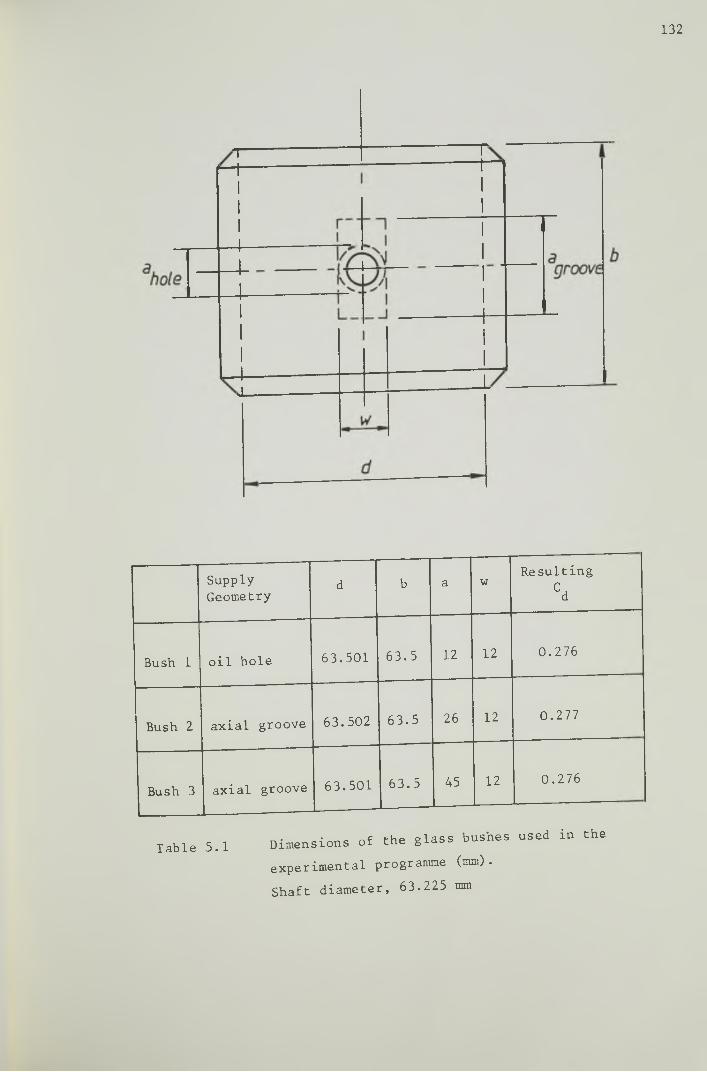
132
Supply
Geometryd b a w
Resulting
Cd
Bush 1 oil hole 63.501 63.5 12 12 0.276
Bush 2 axial groove 63.502 63.5 26 12 0.277
Bush 3 axial groove 63.501 63.5 45 12 0.276
Table 5 .1 Dimensions of the glass boshes used in the
experimental programme (mm).
Shaft diameter, 63.225 mm
133
8mm in diameter. A brass tool of cylindrical shape attached to the head
of a vertical milling machine was then used to machine the axial groove.
This operation is sketched in Figure 5 .2 The length of the tool was the
same as the required groove length ( a ) ; the diameter of the tool was
calculated to give specified values of groove width and depth at the
groove centre. The tools used had a diameter of 18 mm which produced a
groove 12 mm wide with a maximum depth of 2 .3 mm. The bush was clamped
to the universal table of the milling machine which was then moved to
position. The contact surface of the brass tool was fed with Carborundum,
a grinding compound (silicon carbide and grease mixed), while rotating
in contact with the bush surface. The table of the machine was moved
slowly in the horizontal direction (as indicated in Figure 5 .2 ) keeping
the surface of the glass bush slightly pressed against the surface of the
brass tool. The current depth of the groove was equal to the total
displacement of the table.
The technique used with Bushes 2 and 3 to drill the hole for the
lubricant supply pipe, was also employed to drill the oil hole in Bush 1.
A core drill of 12 mm diameter was used. The recess was formed by the
brass pipe when it was glued to the bush. The diameter of the oil inlet
pipe was 6 mm, a value common to all the bushes.
5 .2 .2 The Lubricant Supply System
A line diagram of the lubricant supply system is shown in
Figure 5 .3 . The lubricant used was a Shell oil designated as H .V .I . 60,
a straight mineral oil to which red dye (Waxoline red) was added to
facilitate visual observations of the oil film in the bearing. A screw
pump pumped oil from the supply tank (containing about 12 litres of oil)
to the bearing. The pump had been supplied by Mono Pumps Ltd. with a

134
Machine head
Motion of the brass tool
Table of the machine Direction of displacement of the table
Figure 5 .2 The technique used for machining the
axial groove in a glass bush

135
Figure 5 .3 A line diagram of the lubricant supply
system

136
constant speed electric motor. In the present experimental programme
tests for variable oil supply pressure at fixed values of eccentricity
ratio were performed and the resulting oil flow rate in the bearing
measured. A variable oil supply pressure was achieved by altering the
flow rate delivered by the pump, that i s , by varying the rotational
speed of the oil pump. The constant speed motor supplied with the pump
was, therefore, removed and replaced by a 0.37kW, variable speed motor,
controlled by a Fenner control unit.
It was observed that at supply pressures greater than 1.5-2 bar
(150-200 kN/m ) the flow delivered by the pump was a pulsating one
resulting in oscillations in the value of the supply pressure. To smooth
down the output from the pump a pulsation damper was mounted on the oil
supply circuit. Inside the damper the oil passed through a rubber sleeve
housed in a chamber where there was air under pressure. For the damping
to be effective in the conditions of the experiments the air pressure in
the chamber, which was controlled by a pressure gauge mounted on a pressure
2tapping provided, had to be at least 2 .5 bar (250 kN/m ) .
From the damper the oil was conducted directly to the test
bearing. The oil issuing from the sides of the bearing was discharged
via two holes, one on each side (see Figure 5 .1 ) , into a collecting tray
placed beneath the apparatus from where it was returned by gravity to the
supply tank. A relief valve was installed downstream of the pump.
5 .3 Measurement Techniques
A number of parameters were measured, some were used in a direct
comparison with tha predictions of the theory, others were combined in
dimensionless groups for a comparative study of results for a wide range

137
of operating conditions. The measurement techniques used w ill be discussed
in the following sections.
5 .3 .1 Lubricant Characteristics
The kinematic viscosity of the lubricant was determined by using a
suspended level U-tube capillary viscometer. From a knowledge of the
kinematic viscosity at two different values of temperature an equation for
the viscosity - temperature relationship can be obtained as discussed in
Miranda (1983). For the Shell H .V .I . 60 oil used the following viscosity -
temperature relationship was derived,
log log (v + 0 . 8) = 9 .567 - 3.772 log (t + 273) (5 .1 )
where (v) is the kinematic viscosity of the oil in centistoke and (t) is the
oil temperature in degrees Celsius.
The oil density, required for determining the oil flow rate and
to convert kinematic viscosity to dynamic viscosity, was determined by
using a specific gravity bottle, At a temperature of 19°C the density
was found to be 867.5 kg/m3 . Variations of oil density with temperature
were not significant for the temperature variations observed in the
experiments.
5 .3 .2 Eccentricity Ratio
By design, the value of the eccentricity ratio and the location
of the position of maximum film thickness would be determined by the
thicknesses of the packing blocks and of the packing plate used.
Different sets of packing blocks and packing plates of convenient
thicknesses would allow bush settings at any pre-selected value of
eccentricity ratio. However, during the commissioning of the apparatus
it was found that after a pair of packing blocks had been mounted and

138
the resulting eccentricity ratio checked, i f this pair of packing blocks
was then removed and mounted again the same value of eccentricity ratio
was usually not obtained. This was attributed to the method of holding
the floating bracket which relied on screws tightened up against the
packing blocks and the packing plate and also to the test bush clamping
technique (see Plate 5 .1 and Figure 5 .1 ) . The design technique of setting
the bush for a pre-selected value of eccentricity ratio, was therefore,
not reliable.
All the tests were performed with the oil inlet port located at
the position of maximum film thickness. This permitted the use of sets
of packing blocks of different thicknesses in conjunction with an unchanged
packing plate, in order to obtain variable values of eccentricity ratio.
Four sets of packing blocks which would allow settings with eccentricity
ratios in the range (0.2 - 0 . 8) were manufactured (the pair of packing
blocks and the packing plate which produced a concentric bush-shaft
position were supplied with the apparatus). The pair of packing blocks
with the most suitable thicknesses to produce an eccentricity ratio
approximate to the value required was used and the resulting eccentricity
ratio was determined as follows. The plunger of a clock dial test
indicator (hereafter referred to as dial gauge) was introduced into the
inlet brass pipe of the glass bush to make contact with the surface of the
shaft. The dial gauge was fixed to the bush inlet brass pipe by means of
a sleeve and contact screws as ahown in Plate 5 .2 . The plunger could be
freely moved. A diaplacerent of the plunger was converted into a
rotational movement of the needle of the dial gauge in a circular scale
with 100 divisions, each division corresponding to a displacement of the
plunger by 0 .01 a». When the glass bush was rotated around the stationary
ahaft, the position of maximum clearance could be detected by the change

139
Plate 5 .2 A photograph illustrating the
arrangemen t used to determine
the eccentricity ratio

140
in the direction of movement of the needle of the dial gauge. If (AC)
was the change in the dial gauge reading when the glass bush was rotated
from the positions of maximum to minimum film thickness, the eccentricity
ratio is given by
AC 9\e = 7- (5 .2 )
Ld
5 .3 .3 Rotating Shaft Speed
The rotational speed of the shaft was measured using a hand
mechanical tachometer.
5 .3 .4 Lubricant Supply Pressure
The pressure at which oil was supplied to the bearing was measured
using a Bourdon-tube pressure gauge. A flexible plastic pipe (9 mm in
diameter, 0 .8 m long) connected the point where the pressure gauge was
positioned (see Figure 5 .3 ) with the bush inlet pipe. The pressure drop
in the plastic pipe due to viscous effects was calculated as being of
about 0 .06 bar (6kN/m2) for average operating conditions, a value which
is not significant in comparison with the values of finite supply pressure
used in the experiments.
5 .3 .5 Lubricant Temperatures
The oil temperature was measured by nickel-chromium/nickel-aluminium
thermocouples in conjunction with a ’ Comark' electronic thermometer. The
zero temperature reading was checked by a thermocouple immersed in a bath
of iced water.
The temperature of the side leakage oil was measured by
thermocouples positioned in the holes which conducted the oil to the
Electing tray. For the measurement of the inlet temperature of the oilCOJ
141
a thermocouple was positioned just upstream of the bush inlet brass pipe.
Measurements of the oil inlet temperature were only performed in the
commissioning tests. Oil film temperatures were not measured.
5 .3 .6 Lubricant Flow Rate
A comparison of experimental results of side flow rate with
theoretical predictions was one of the main aims of the experimental
programme. The method used to measure the side flow rate was simple and
reliable; the oil discharged from the sides of the bearing during an
interval of tine (At) was collected in a portable tray the weight of
which, when empty, had been previously measured. The time of oil collection
was measured using a stop watch and was normally of 60 seconds and 30
seconds at low and high values of oil supply pressure respectively. The
tray containing the oil collected was then weighed and the weight of the
oil collected determined. The side flow rate was evaluated from a knowledge
of the weight of the oil collected, the time interval (At) and the oil
dens i ty .
5 . 3 . 7 Location of the Rupture and the Reformation Boundaries
The datum for the angular location of the rupture and the
reformation boundaries was the position of the groove (or of the oil hole)
which was located at the maximum film thickness. A scale graduated in
degrees was engraved on one of the brass clamp sleeves holding the glass
bush. The zero of the scale was in the top vertical position and the
cale was graduated from 0° to 180° in the direction of greater visibility ,
and from 0° to 90° in the opposite direction. The smallest division of
the scale corresponded to an angular change of 5 .
S(

142
5 .4 The Commissioning of the Apparatus
5 .4 .1 Observations
To find out whether the apparatus was functioning as designed,
introductory testing was performed without recording any results. Variable
values of eccentricity ratio could be obtained using different sets of
packing blocks. Repeatability in the value of the eccentricity ratio for
the sane pair of packing blocks was, however, not normally achieved as
discussed in Section 5 .3 .2 . The location of the position of maximum film
thickness, as well as the eccentricity ratio, could be determined using a
dial gauge. The maximum error in the location of the position of maximum
film thickness was estimated as being of ±5 and ±10 at high and low
values of eccentricity ratio respectively.
A variable flow rate was obtained by varying the rotational speed
of the oil pump - No visible fluctuation in the oil flow rate issuing
from the open end of the supply pipe was observed. With the supply pipe
connected to the bearing, oscillations of the needle of the pressure gauge
were noticeable at supply pressures greater than 1.5-2 bar (150-200 kN/m )
increasing in amplitude as the supply pressure increased. This fluctuation
in the value of supply pressure, due to a pulsating delivery from the oil
pump, was completely eliminated when a pulsation damper was installed as
discussed in Section 5 .2 .2 .
Film rupture and film reformation could be observed as well as the
effect of oil supply pressure on the location of the film reformation
boundary. For some bush settings it was observed that the reformation
boundary was clearly assymetrical with respect to the bearing centre line;
this was caused by misalignment between the bush and the shaft axes.
Thermal equilibrium was generally achieved after a 4 - 5 hours

143
run at constant operating conditions. At a shaft speed of 600 r .p .m .
2(10 Hz) and oil supply pressure of 1 bar (lOOkN/m ) , the observed increase
in the temperature of the oil after thermal equilibrium had been reached
was about 10°C when the shaft ran concentric with the bush, and of about
12 C at an eccentricity ratio of 0 .7 6 . The rise in the temperature of
the oil as it passed through the test bearing was about 1 C at concentric
shaft/bush and about 2°C at e=0.76 . It is worth noting here that the
effective temperature of the oil in the bearing was assumed to be equal
to the measured outlet temperature for the purpose of calculating the
dimensionless supply pressure.
Despite the difficulties encountered in setting the test bearing
for pre-selected values of eccentricity ratio and to achieve a satisfactory
alignment between the shaft and the bush axes, the apparatus was operating
satisfactorily.
5 .4 .2 Commissioning Tests
Two tests were carried out, both with Bush 3 with the groove located
at the position of maximum film thickness, for a comparison of experimental
flow rates with theoretical predictions from other sources. A first test
was run with the shaft stationary. The oil flow rate at four values of
supply pressure in the range 0.68-1.69 bar (68 - 169 kN/m2) was measured
for each value of eccentricity ratio tested. Figure 5 .4 shows a comparison
of the experimental results of dimensionless flow rate with the theoretical
predictions of ESDU Item No. 66023 (1966) and Martin and Lee (1982).
The flow rate was made dimensionless according to the expression shown in
the same figure. The experimental results at a fixed value of (e) varied
slightly with the value of supply pressure (pf) . Very good correlation
was achieved, the biggest percentage difference observed being 34.3% at

Dimen
sionle
ss
Flow
Rate,
Q'=
Q
rj /p.
144
Figure 5 .4 A comparison of the experimentally determined
dimensionless flow rate when using Bush 3 with
a stationary shaft, with the theoretical
predictions of ESDU Item No. 66023 (1966) and
Martin and Lee (1982)
145
£=0.65. Errors in the location of the position of maximum film thickness
and bearing misalignment were probably the cause for the discrepancies
observed.
A second test was run at fixed values of eccentricity ratio and
oil supply pressure and at variable shaft speed. Figure 5 .5 shows the
correlation observed between the experimentally determined side flow
rate and the theoretical predictions of ESDU Item No. 66023 (1966). Again,
very good agreement was observed the maximum difference being 14.9%.
The very good correlation between experimental results and
theoretical predictions of other sources achieved in those two tests
indicated that the apparatus could be used with confidence to obtain
experimental results for a wide range of operating conditions. An
experimental programme was carried out in order to study the correlation
between experiment and the predictions of the theoretical analysis presented
in this thesis. A discussion of results of the experimental programme will
be dealt with in the next chapter.
5 .5 Conclusions
(1) An apparatus for the study of oil flow in journal bearings has been
designed. The use of glass bushes permitted a visual study of the
film extent in the bearing.
(2) The commissioning of the apparatus has been performed. Operation at
a wide range of conditions was possible and the effect of operating
parameters on flow rate and on the location of the film reformation
boundary was observed to be as expected.
It was found that it was difficult to establish a bush setting for a
pre-selected value of eccentricity ratio and a careful setting was

Side
Flow
Rate
x 10
(m /s
)
146
Figure 5 .5 A comparison between the experimentally
determined side flow rate and the predictions
of ESDU Item No. 66023 (1966), with Bush 3
at fixed eccentricity ratio and oil supply2
pressure (e = 0 .6 7 , pf = 1.69 bar (169 kN/m )

147
required to minimize bearing misalignment. However, this would not
affect the aims of the experimental programme.
Preliminary tests have been performed which gave very good
correlation between the experimentally determined side flow rate and
the theoretical predictions of ESDU Item No. 66023 (1966) and Martin
and Lee (1982).
The commissioning of the experimental apparatus has confirmed that it
could be used with confidence to carry out a programme of tests.
148
CHAPTER 6
THE EXPERIMENTAL PROGRAMME
AND DISCUSSION OF RESULTS
6 .1 Introduction
The experimental apparatus has been described in Chapter 5 . The
commissioning tests carried out identified some limitations of the
apparatus, for example a difficulty in obtaining a bearing setting
corresponding to a pre-selected value of eccentricity ratio, and also
showed that a very careful bush setting was required to minimize axial
misalignment and to prevent errors in the determination of the operating
eccentricity ratio and in the location of the position of the maximum
clearance. Misalignment affects the flow rate of lubricant in the
bearing (Hargreaves (1981), Siew and Reason (1982)) and in addition it
would affect the measurements of the angular extent of the full film
region in the present experiments.
The results of the commissioning tests showed good correlation
with theoretical predictions from other sources, indicating that the
apparatus could, nevertheless, be used with confidence to provide a wide
range of experimental results for comparison with the predictions of the
present theoretical analysis. For this purpose a detailed programme of
tests was prepared.

149
This chapter will deal with the experimental programme and a
discussion on the correlation between the experimental results and the
theoretical predictions.
6 .2 The Experimental Programme
The computer program used in the present journal bearing analysis
was able to generate solutions for a range of values of bearing width-to-
diameter ratio (b /d ) , eccentricity ratio ( e ) , groove length-to-bearing
width ratio (a /b ) , groove width-to-bearing diameter ratio (w/d) and
dimensionless supply pressure (p ^ ). The bushes used in the experiments
had fixed values for ( b ) , (d ) , (w) and (C ,) as indicated in Table 5 .1 .a
The parameters (b /d ) , (w/d) and (C ./d ) were therefore the same for alld
bushes. The length of the groove (a) varied from bush to bush. The
operating eccentricity ratio and the dimensionless supply pressure could
of course be varied. Table 6 .1 gives the values of the bearing parameters
corresponding to each bush tested (based on the bearing dimensions shown
in Table 5 .1 ) .
Supply
geometryb/d C Jd
aa/b w/d
Bush 1 oil hole 1 4.365xlO_3 0.189 0.189
Bush 2 axial groove 1 4 . 365xlO~3 0.409 0.189
Bush 3 axial groove 1 4.365x10 0.708 0.189
Table 6 .1 Bearing parameters and groove size
corresponding to each bush used in
the experiments

150
To allow a comparison of results over a wide range of operating
conditions to be carried out, the experiments were programmed in a way
that permitted the results to be expressed in dimensionless form whenever
possible.
The parameters that could be varied in the tests were the
eccentricity ratio and the dimensionless supply pressure. The latter
was dependent on the oil supply pressure, on the shaft speed and on the
effective temperature of the o il . The oil supply pressure and the shaft
speed were set, the oil temperature was measured. Tests involving the
three bushes provided results at variable (a /b ) .
Two sets of experiments were carried out. The tests included in
the 'set of experiments X' involved all three bushes and were performed
at fixed journal speed. Each bush was usually set to six different
values of eccentricity ratio in the range (0 .2 —0 .8 ) . For each bush
setting tests for four values of oil supply pressure were carried out.
The 'set of experiments 2' involved only one bush and was designed to
show the effect of shaft speed on the bearing performance. The tests
were carried out at fixed eccentricity ratio for five values of shaft
speed, in the range 200—1000 r.p .m . (3 .33—16.66 Hz), and at two
different values of oil supply pressure. Table 6 .2 gives the details
of the programme of tests.
6 .2 .2 The Test Procedure
The apparatus was assembled as described in Chapter 5 . The test
procedure was as follows.
6 . 2 . 1 The Tests
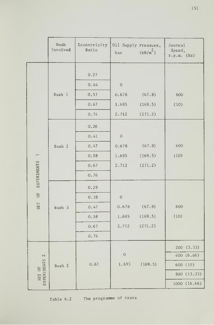
151
Bush
Involved
Eccentricity
Ratio
Oil Supply
bar
Pressure,
(kN/m )
Journal
Speed,
r.p .m . (Hz)
0 .27
0 .44 0
Bush 1 0 .57 0 .678 (67 .8) 600
0.67 1.695 (169.5) (10)
0 .74 2.712 (271.2)
0 .26
0 .41 0
Bush 2 0.47 0.678 (67.8) 600
i-H 0 .58 1.695 (169.5) (10)
c/iHas 0.67 2.712 (271.2)
MPiW
0.76
CL,X!w 0.29
toO 0 .38 0
SET
Bush 3 0.47 0 .678 (67 .8) 600
0 .58 1.695 (169.5) (10)
0.67 2.712 (271.2)
0 .74
200 (3 .33)
CM 0 400 (6 .66)
HBush 2 0.67 1.695 (169.5) 600 (10)
Ht -t e£ w wCA Cu
X W
800 (13 .33)
1000 (16 .66)
Table 6 .2 The programme of tests

152
(1) The 'adjustment screws' were unscrewed to make sure that they were
not operating. The 'clamping screws' were tightened up gently
pulling the bush holders against the bush. At the end of this
operation the bush should not be loose but should be able to be
rotated over its tapered ends.
(2) The pair of packing blocks which was supposed to provide a setting
with the closest value of eccentricity ratio to the one desired,
were screwed tight in place.
(3) A dial gauge was used to detect the position of maximum film
thickness and to measure the change in clearance from this position
to the position of minimum film thickness. The value of the
eccentricity ratio was calculated from a knowledge of this change
in clearance, as discussed in Chapter 5 (Section 5 .3 .2 ) .
(4) 'Adjustment' and 'clamping' screws were altered until a suitable
value of eccentricity ratio was achieved.
(5) The oil groove was centered in the position of maximum film
thickness and a little action on one of the 'adjustment or of the
'clamping' screws usually sufficed for holding the bush tight in
that position.
(6) The dial gauge was then taken off the bush inlet brass pipe and the
oil supply pipe was connected to the bearing. A clamp was used
to prevent separation of the plastic pipe from the inlet brass pipe
at high oil supply pressures.
(7) The oil pump drive motor and the shaft drive motor were switched on
and operated at a low speed to check the bearing misalignment.
The procedure returned to step (4) until acceptable bearing
alignment was achieved. Sometimes this proved to be a tedious and

153
time-consuming operation
(8) The shaft speed was set to the required value and the rotational
speed of the oil pump was then altered until the desired value
for the oil supply pressure was indicated by the pressure gauge.
The shaft speed was checked regularly during the tests.
(9) The measurements required were recorded.
(10) Once the tests with the current bush setting had been completed
the eccentricity ratio was checked with the dial gauge. The value
for eccentricity ratio measured after the tests was, in general,
not significantly different from the one corresponding to the initial
setting. The eccentricity ratio adopted for that set of tests was
the mean of the two values measured.
6 .2 .3 The Measurements Recorded
During the setting up of the bush two measurements were recorded:
(i) The angular location of the position of maximum film thickness
(11) The change in clearance from the position of maximum to the
position of minimum film thickness which allowed the
determination of the eccentricity ratio.
For a given bush setting the following measurements were recorded
during every test:
(i ii ) The rotational speed of the shaft
(iv) The oil supply pressure
(v) The weight of the collected side leakage oil and the time in which
it was collected. This allowed the determination of the side flow
rate as discussed in Chapter 5 (Section 5 .3 .6 ) . In order to
compare the experimental results for side flow with the theoretical
predictions the flow rate measured was usually normalized according
154
to the expression adopted in this thesis.
(vi) The location of the rupture and of the reformation boundaries. The
location of a boundary was defined by an angle measured from the
groove centre line to the boundary in the direction of the shaft
rotation. The groove was assumed to be located at the position of
maximum film thickness. The angular location of the rupture boundary
was recorded as an angle (&c) measured at the bearing centre line.
At low oil supply pressures the upstream end of the full film
region usually coincided with the upstream edge of the groove.
In such a situation only the angular location of the beginning of
the full width film (a » at the bearing edge) was recorded. When,
at moderate/high values of supply pressure, the reformation
boundary was located upstream of the groove (see Plate 6 .1 ) both
(a ) and the angular location of the nose of the boundary (at the
bearing centre line) were recorded.
(vii)The outlet temperature of the oil. It has been pointed out in
Chapter 5 that oil temperatures could take four hours to stabilize
under constant operating conditions. The operating conditions
changed from test to test due to changes in oil supply pressure or
shaft speed (see Table 6 .2 ) and it would have been impractical to
wait until a stabilized temperature had been reached in every test.
On the other hand, the rate of increase in the oil temperature at
given operating conditions was usually small and, therefore, in the
period of time required to collect the oil and to read out the
angular location of the boundaries of the cavitation region, the
observed increase in temperature was not significant (0 .5 °C was the
maximum increase observed). Two readings of the outlet temperature

155
of the oil were recorded; the first was taken immediately before
and the second was taken immediately after the collection of the
oil and the reading of the angular location of the boundaries of
the cavitation region. The oil outlet temperature was taken as the
mean of those two readings and was assumed to be equal to the
effective temperature of the oil for the purpose of determining the
dimensionless supply pressure.
6 .3 Experimental Results and Discussion
The main purpose of this experimental programme was to provide
results for comparison with the predictions of the theoretical analysis
discussed in this thesis. The use of glass bearings enabled the
visualization of the film of oil in the bearing. The effect of the
operating conditions on the extent of the full width film was investigated
and other qualitative observations recorded.
The remainder of this chapter will be concerned with some
experimental observations and with a comparison of experimental results
for side flow rate and for the location of the rupture and the
reformation boundaries, with the predictions of the theoretical analysis.
6 .3 .1 Qualitative Observations
In the tests carried out with Bush 1 (oil hole) at low values
of eccentricity ratio (e < 0 .3 ) and at constant shaft speed (600 r.p.m .
(10 Hz)) a complete film of oil was observed all around the bearing
at any of the supply pressures tested. When the speed was increased
a value was reached at which air bubbles appeared in the divergent film
region of the bearing completely surrounded by a complete film of oil.
This minimum value of shaft speed was dependent on the supply pressure
and decreased as the latter increased. Some of the air forming these
air bubbles, which were not fixed in position, had been driven along

156
by the oil supply stream and moved upstream after leaving the oil groove.
In the experiments involving Bush 2 (axial groove, a/b = 0.409) at £ =
0.26, air bubbles appeared in the region upstream of the groove when the
supply pressure was greater than the ambient. At zero supply pressure a
complete film of oil around the bearing occurred. With Bush 3 (axial
groove, a/b = 0.708) at £ = 0.29, air bubbles were observed in the
divergent region of the bearing at all supply pressures tested.
As the eccentricity ratio was increased a well defined cavitation
region was observed in all tests where the rupture and the reformation
boundaries could be identified clearly. If some axial misalignment
between bush and shaft existed it would be detected by the lack of
symmetry of the film pattern in the cavitation zone with respect to the
bearing centre line and, in particular, by the shape of the reformation
boundary.
In the cavitation region all the oil appeared to be carried over
by the oil streamers and none between the air cavities and the moving
shaft.
Whilst the rupture boundary was more or less straight, the
reformation boundary at either low or high supply pressure conditions had
a curved shape very similar to that predicted by the theory. Plate 6.1
shows the experimentally observed reformation boundaries and the
corresponding theoretical predictions at two different sets of operating
conditions.
The influence of the oil supply pressure on the extent of the
complete width film was clearly seen in the tests involving Bush 1 (oil
hole) and Bush 2 (.axial groove, a7b - 0.409). At given shaft speed and
eccentricity ratio, the supply pressure being the ambient, the cavitation
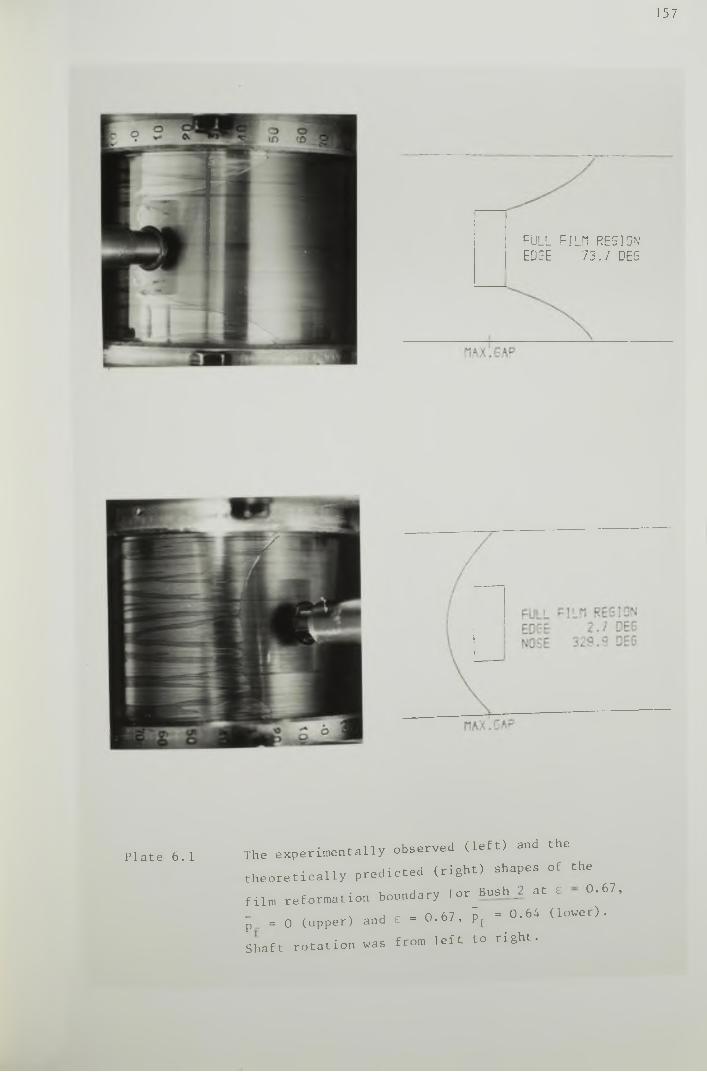
157
Plate 6.1 The experimentally observed (left) and thetheoretically predicted (right) shapes of the film reformation boundary for Bush_2 at e - 0.67, | = o (upper) and e ■ 0.67, | =0.64 (lower). Shaft rotation was from left to right.
FULL FILM REGION EDGE 73.7 DEG
158
region extended well downstream of the groove. As the supply pressure
increased the reformation boundary moved upstream due to the increased
inlet flow of oil (see Figure 6.7). The location of the rupture boundary
was not significantly affected by changes in oil supply pressure, an
observation that is in agreement with the theoretical predictions (see
Appendix C).
When running tests at variable speed a stable film reformation
boundary was observed for all speeds tested at low values of supply
pressure. At the higher values of supply pressure, however, an
instability was observed at the air-oil interface in the film reformation
zone characterized by the local break down of the air-oil interfaces
due to what seemed to be the collapse of air bubbles carried by the oil
inlet stream and moving upstream from the groove to the film reformation
boundary. At given values of eccentricity ratio and oil supply pressure
there existed a value of shaft speed above which this instability
occurred. This phenomenon has also been observed by Cole and Hughes (1956)
and Hargreaves (1981).
6.3.2 Interpolation of the Experimental Results
Experimental results were obtained for the range of operating
conditions shown in Table 6.2. The tests included in the 'set of
experiments 1* were designed to give results for dimensionless side
flow rate and for the location of the rupture and of the reformation
boundaries at constant shaft speed and variable eccentricity ratio and
oil supply pressure. For a given test bush (fixed(a/b)) and at fixed
eccentricity ratio, results were obtained at four values of oil supply
pressure. A convenient way of presenting a comparison of experimental
results with theoretical predictions seemed to be the graphical form
with the dimensionless supply pressure as the parameter, incorporating
159
the rotational speed, the oil supply pressure and the effective
temperature of the oil. Although the speed was the same for all
tests and the same values of supply pressure were used at each eccentricity
ratio, the values for dimensionless supply pressure (corresponding to
a given value of oil supply pressure) calculated at two different
values of eccentricity ratio, usually differed due to differences in
the effective temperature of the oil. To convert experimental
results at variable values of eccentricity ratio and variable determined
dimensionless supply pressure into results at variable eccentricity
ratio and pre—fixed values of dimensionless supply pressure,
graphical interpolation was used for every value of the eccentricity
ratio. The procedure was as follows.
(i) Experimental results for dimensionless side flow and for the
location of the rupture and of the reformation boundaries were
plotted against the experimental values of dimensionless supply
pressure. These plots were usually straight lines for the
dimensionless flow rate and smooth curves for the location of the
rupture and of the reformation boundaries.
(ii) The required interpolated values corresponding to pre-fixed values
of dimensionless supply pressure (0, 0.5, 1.0 and 1.5) were then
simply read out on the diagram.
An alternative to interpolation of experimental results was the
adjustment of the values of shaft speed and/or oil supply pressure such
that when combined with the measured effective temperature they resulted
in a pre-fixed value of dimensionless supply pressure. This method was
not adopted because it would have required more or less complicated
calculations 'on the spot* with the additional difficulty of a non
stabilized effective temperature of the oil.

160
For the presentation of the experimental results obtained at
fixed eccentricity ratio interpolation was not required.
6.3.3 Lubricant Flow Rates
Results of lubricant side flow rate for all bushes at variable
values of eccentricity ratio and oil supply pressure were obtained from
the 'set of experiments 1*. Based on these, results of dimensionless
side flow rate at pre-selected values of dimensionless supply pressure
(0.0, 0.5, 1.0 and 1.5) and for the same values of eccentricity ratio
as used in the experiments were determined by interpolation as
discussed in Section 6.3.2. The interpolated experimental results
were then compared with the predictions of the theoretical analysis
presented in this thesis.
Figures 6.1 to 6.3 are plots of dimensionless side flow rate
against eccentricity ratio for four values of dimensionless supply
pressure. Very good correlation has been achieved for all bushes.
The theoretical results for Bush 1 were obtained with the assumption of
a 'square hole' of dimensions equal to the diameter of the oil hole
of the bush, a condition which was expected to cause slightly greater
theoretical predictions of dimensionless flow rate at supply pressures
greater than the ambient. At = 0.5 the maximum percentage difference
observed between the interpolated experimental results and the
theoretical predictions was 17.2%. At higher values of dimensionless
supply pressure the correlation was better with a maximum discrepancy
of 12.7% at pf = 1-5.
With Bushes 2 and 3 very good correlation was achieved at low
«■ . . nressure CO.O and 0.5) for all values ofdimensionless supply pressure. . „• At- hieher values of CpJ with Bush 2 theeccentricity ratio. At nignei v<*
• foi rpcnits showed some scatter, the biggest deviation from the experimental results shuwcu
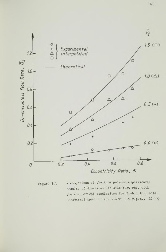
Dim
ensi
onle
ss
Flow
R
ate
,
161
Figure 6.1 A comparison of the interpolated experimental results of dimensionless side flow rate with the theoretical predictions for Bush 1 (oil hole). Rotational speed of the shaft, 600 r.p.m., (10 Hz)
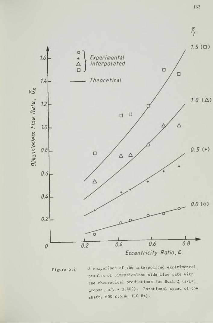
Dim
ensi
onle
ss
Flow
R
ate
.
162
pf
Figure 6.2 A comparison of the interpolated experimentalresults of dimensionless side flow rate with the theoretical predictions for Bush 2 (axial groove, a/b = 0.409). Rotational speed of the shaft, 600 r.p.m. (10 Hz).

Dim
ensi
onle
ss
Flow
R
ate
,
163
Eccentricity R atio , &
Figure 6.3 A comparison of the interpolated experimental results of dimensionless side flow rate with the theoretical predictions for Bush 3 (axial groove, a/b. = 0.708). Rotational speed of the shaft, 600 r.p.m. (10 Hz)

164
theoretical predictions being of 22.8% at p - 1.5. With Bush 3 the
experimental results at high values of (p^) were consistently greater
than the theoretical predictions, the differences being more significant
at low values of (e). The results exhibited the same trend as the
theoretical predictions with a maximum percentage difference of 27.1%
at p. = 1.5 and e = 0.29.
Possible errors in the location of the position of maximum
film thickness and in the determination of the eccentricity ratio could
have been partly responsible for the deviations from the theoretical
predictions observed. Misalignment was, however, thought to have
caused most of the discrepancies. Hargreaves (1981) showed that
misalignment would result in an increase in oil flow rate. When
misalignment existed its effect on the measured flow rate would become
increasingly significant at increasing values of dimensionless supply
pressure.
Figures 6.1 to 6.3 also show the dependence of dimensionless side
flow rate on eccentricity ratio, groove size and dimensionless supply
pressure. The effect of the rotational speed of the shaft on side flow
rate is shown in Figure 6.4 for two values of oil supply pressure, namely,2ambient and 1.695 bar (169.5 kN/m ). The experimental results were
obtained with Bush 2 at fixed £ = 0.67. The increase in the outlet
temperature of the oil observed during the tests was, 1.3 C and 2.5 C
at the ambient supply pressure and at p^ — 1.695 bar respectively.
The effect of these relatively small changes in oil temperature on the
side flow rate was negligible in comparison with the effect of shaft
speed. Very good correlation with the theoretical predictions was
achieved. At the supply pressure of 1.695 bar (169.5 kN/m2) the
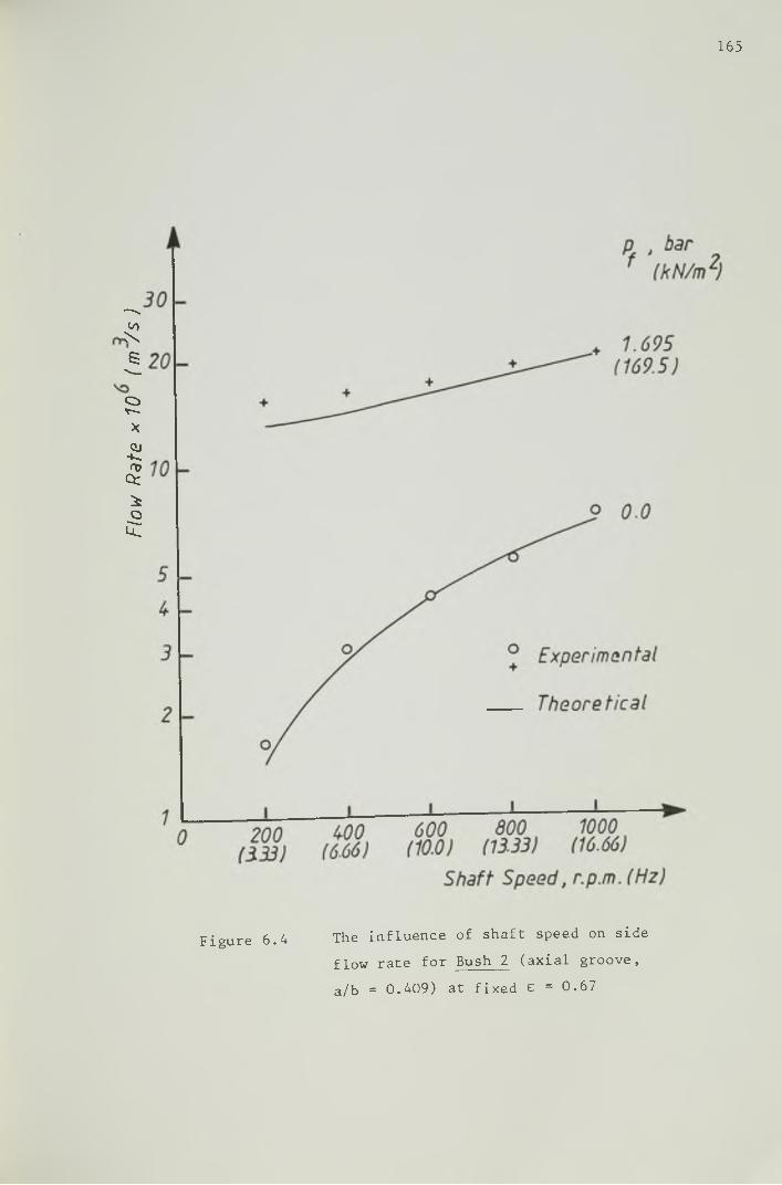
Flow
Ra
te
* 10
(m /s
)
165
Figure 6.4 The influence of shaft speed on side flow rate for Bush 2 (axial groove, a/b = 0.409) at fixed £ = 0.67

166
experimentally determined oil flow rates were all greater than the
theoretical predictions, the maximum percentage difference being of
14.2% at the lowest value of the shaft speed. This small discrepancy
could again be due to some degree of bearing misalignment.
When the differences between the results for side flow rate2at the supply pressure of 1.695 bar (169.5 kN/m ) and at the ambient
supply pressure were calculated for all values of shaft speed tested,
it was found that those differences were all within the range (13.49 x~6 - ^ 310 - 14.17 x 10 m /s). This supports the approach adopted by
some journal bearing design procedures in which the side flow rate
is calculated aS the sum of two flow components: a ’zero supply pressure
flow' which is not dependent on the oil supply pressure and a 'zero
velocity flow' which depends on the oil supply pressure and is
calculated assuming a stationary journal.
6.3.4 The Location of the Film Rupture and the Film Reformation
Boundaries
The measurements recorded concerning the location of the film
rupture and the film reformation boundaries have been discussed in
Section 6.2.3. A comparison of the experimental results for the angular
location of the beginning of the full width film (0 ) and for the angular
location of the film rupture boundary (01 ), with the theoretical
predictions was carried out for all the experimental results obtained.
The correlation observed in the comparison of results for the various
bushes was qualitatively similar, hence results obtained with one bush
only will be presented in each case.

167
Figure 6.5 shows a comparison of the interpolated experimental
results for the location of the film reformation boundary with the
theoretical predictions at fixed shaft speed. Very good correlation
was achieved at high values of dimensionless supply pressure for all
values of eccentricity ratio. The experimentally determined values
of (a) were consistently lower than the theoretical predictions at low
and moderate values of (e) and were higher than the theoretical
predictions at high values of (e). This trend was also observed with
Bush 1 and with Bush 3. The maximum discrepancies observed at high
values of (p^) were 7° and 5 at p^ = 1.0 and p^ = 1.5 respectively.
At p^ = 0 and p^ = 0.5 correlation was good at high values of (e).
Maximum differences of about 20° were observed at low values of (e).
At e > 0.5 the maximum discrepancy observed was 9° and 6° at p = 0
and p^ = 0.5 respectively.
Possible sources of error in the measurement of the angular
location of the rupture and of the reformation boundaries were:
(i) Bearing misalignment
Imprecise location of the position of maximum film thiclcness. An
estimate of the maximum error introduced by this means was ± 10
at low values of (£) and ± 5 at high values of (£).
(iii) The fact that the bearing edge could not actually be seen due to
the bush clamping technique used. The location of the point on
the bearing edge where a full width film occurred was estimated
by visual extrapolation.
(iv) The instability observed at the downstream end of the air cavities under particular operating conditions discussed in Section 6.3.1.
This could affect the identification of the real reformation boundary.

Ref
orm
atio
n Bo
unda
ry
Loca
tion
, ar
(de
gre
es)
168
A } ^interpolated region / / \ \ _ \ reQl0n n )
/ / Z / V / V w Theoretical
Figure 6.5 A comparison of the interpolated experimentalresults for the location of the film reformation boundary with the theoretical predictions for Bush 2 (axial groove, a/b = 0.409). Shaft speed 600 r.p.m. (10 Hz)
169
(v) Approximations associated with the interpolation of experimental results.
It was felt that causes (i) and (ii) were the major sources of
errors in the experimental results under discussion.
The discrepancies observed in Figure 6.5 at e < 0.5 for p = 0
and p^ = 0.5 occurred with the tests on all bushes and in all cases
the experimental results were lower than the theoretical predictions.
It did not seem reasonable to attribute those differencies to the
possible causes of error enumerated above. It is worth noting that
very good agreement in dimensionless side flow rate was achieved at
all values of (e) for p^ = 0 and p^ = 0.5 (see Figure 6.2). A plausible
explanation for these discrepancies could not be found.
Figure 6.6 shows a comparison of the experimental results for
the angular location of the film rupture boundary (oi ) with the
theoretical predictions, observed with Bush 3. The experimentally
determined values of (oc ) were not significantly affected by the oilcsupply pressure. The theoretical predictions showed a very slight
variation of (a ) with (pj for a given (e). The solid curve represented c £in Figure 6.6 gives the theoretical predictions for all values of (pf)
with a maximum error of 3.5°. Large experimental discrepancies (within
the range 30°-42°) with the theoretical predictions were observed at all
values of eccentricity ratio. They could be partly due to experimental
errors but it was belived that they were mainly a result of the physical
model for film rupture adopted and incorporated in the theoretical analysis.
Elrod's cavitation algorithm, which formed the basis of the present
theoretical analysis, incorporated the Reynolds boundary conditions which
assume that pressure and pressure gradients take the value zero at the

Rupt
ure
Boun
dary
Lo
cati
on
, a
(de
gre
es)
170
Eccentricity Ratio, &
Figure 6.6 A comparison of the experimental results for the location of the film rupture boundary with the theoretical predictions for Bush 3 (axial groove, a/b = 0.708) at all values of supply pressure. Shaft speed, 600 r.p.m. (10 Hz).

171
film break down. Although commonly used, the Reynolds boundary conditions
for film rupture cannot predict the negative pressure loop which has been
observed by a number of researchers immediately upstream of film break down
(McKee and McKee (1932), Dowson (1957), Floberg (1965), Etsion and Ludwig (1982)).
The occurrence of a sub-ambient pressure loop results in an extended
full film region in comparison with theoretically predicted by solutions
incorporating Reynolds' conditions. Theoretical models for film rupture
have been presented also by Floberg (1965, 1968) and Coyne and Elrod
(1970, 1971) both predicting a sub -cavity pressure loop upstream of the
cavitating region. Taylor (1973) investigated the effect of the
theoretical model used on the prediction of the angular location of the
film rupture boundary for infinite width journal bearings. The boundary
conditions considered were the Reynolds boundary conditions and a
condition derived from a flow separation theory presented by Birkhoff and
Hays (1963) which assumes a full width film and no liquid-gas interface
(this theory was later extended by Coyne and Elrod (1970, 1971) to consider
the presence of a liquid-gas interface). The comparative results showed
that by using the separation condition the angular location of the rupture
boundary was extended by as much as 60 at £ = 0.4 and 25 at £ = 0.7, in
comparison with the results obtained using Reynolds conditions. These
results seemed to indicate that the large differences observed in Figure
6.6 were mainly attributable to the rupture boundary conditions
incorporated in the theoretical analysis.Using Coyne and Elrod (1970, 1971) flow separation conditions
at film rupture, Taylor (1975) carried out a theoretical analysis of
infinite width journal bearings and found that there exists a minimum
value of eccentricity ratio below which separation does not occur.It h a s b e e n pointed out in Section 6.3.1 that cavitation was not
observed in some experiments with Bush 1 and Bush 2 contrary to the

172
predictions of the present theoretical analysis. The findings of
Taylor (1975) show that such a situation can be predicted theoretically
by using more appropriate rupture boundary conditions. If a rupture
cavitation boundary does not occur below a certain value of (e) a
reformation boundary will not occur below the same value of (e). It
would be interesting to know what would be the predictions of (cx ) from
a theoretical analysis incorporating both the Coyne and Elrod (1970,
1971) rupture boundary conditions and the Jakobsson and Floberg (1957)
reformation boundary conditions, as (e) gradually increases, and if
this could provide some explanation for the large discrepancies observed
in Figure 6.5 at low values of (e ) and (p^) •
The Influence of Dimensionless Supply Pressure on the Location of the
Film Reformation Boundary
Figure 6.7 shows the effect of dimensionless supply pressure on
the location of the film reformation boundary for Bush 1 at £ = 0.74 and
a shaft speed of 600 r.p.m. (10 Hz). The correlation between the
experimental results and the theoretical predictions was good. A maximum
discrepancy of 11° was observed at pf = 0.384 and could probably be due
to some of the possible causes of errors already discussed.
The results shown in Figure 6.7 are consistent with the results
for dimensionless flow rate shown in Figure 6.1 corresponding to the
maximum value of (£) tested (£ = 0.74); the experimentally determined
dimensionless side flow rate was always smaller than the theoretical
predictions and it is interesting to note that the biggest discrepancy
occurred at a value of (pf) approximately equal to the one that
produced the biggest discrepancy in Figure 6.7.

Refo
rmat
ion
Boun
dary
Lo
catio
n ,
a (d
egre
es)
173
Figure 6.7 The influence of dimensionless supply pressure on the location of the film reformation boundary. Bush l(oil hole). Shaft speed, 600 r.p.m. (10 Hz). Eccentricity ratio, £ = 0.74

174
The Influence of Shaft Speed on the Location of the Film Reformation
Boundary
The effect of shaft speed on the angular location of the film
reformation boundary is shown in Figure 6.8 for Bush 2, at two values
of oil supply pressure and fixed e = 0.67.
According to the prediction of the theoretical analysis, at
constant ambient supply pressure the value of (a ) should be independent
of the rotational speed of the shaft. The experimental results showed
approximately the same trend with discrepancies similar in magnitude
to those observed in Figure 6.5 at p^ = 0 and £ > 0.5. At a constant2supply pressure of 1.695 bar (169.5 kN/m ) increasing values of speed
resulted in decreasing values of dimensionless supply pressure which
varied from 2.697 to 0.738 during the test. A maximum discrepancy of
16° between the experimentally determined and the theoretically predicted
values of (a ) was observed at a shaft speed of 800 r.p.m. (13.33 Hz), rAt speeds greater than 600 rp.m. (10 Hz) the instability of the film
immediately upstream of the reformation boundary already discussed was
observed and might have affected the identification of the reformation
boundary.
The experimental results for (ar) were lower than the
theoretical predictions for all values of shaft speed. Again this is
consistent with the correlation observed in Figure 6.4 for side flow
rate at the same operating conditions.
6.4 Conclusions
The experimental programme has been outlined in this chapter and
a comparison of experimental results and theoretical predictions
discussed. The following conclusions can be made.

Refo
rmat
ion
Boun
dary
Lo
cati
on
, d
(deg
rees
)
175
Figure 6.8 The influence of shaft speed on the location of the film reformation boundary.Bush 2 (axial groove, a/b = 0.409) Eccentricity ratio, e = 0.67

176
(1) Despite the limitations of the experimental apparatus it was
possible to carry out the experimental programme as planned.
Tests were performed with three bushes of different groove sizes.
The parameters that could be varied were the eccentricity ratio
(e), the dimensionless supply pressure (p^) and the groove
length-to-bearing width ratio (a/b) by using different bushes.
The fixed parameters were b/d = 1 and w/d = 0.189. The groove
was located at the position of maximum film thickness.
(2) Correlation between the experimentally determined dimensionless
flow rate and the theoretical predictions was shown to be very good.
With Bush 1, the maximum percentage difference observed was 17.2%
at pf = 0.5 and e = 0.67. Results obtained with Bush 2 and Bush 3
showed very good correlation with the theoretical predictions
especially at low/moderate values of dimensionless supply pressure.
At high values of (p£) 3nd low eccentrcity ratio the correlation
was not so good, the maximum percentage differences were 22.8%
at ” _ an<j e = 0.41 with Bush 2, and 27.1% at pf = 1.5 and
e = 0.28 with Bush 3.
The possible sources of error in the experimental results have
been discussed, the most influential was believed to be bearing
misalignment.
The good correlation achieved in the present study between
theory and experiment for dimensionless flow rate is certainly a
result of a consideration of the lubricant inlet conditions in the
theoretical analysis. Most predictions of side flow rate presented
in the past have been based on solutions which did not incorporate
the lubricant inlet conditions, and this has been recognized by a
177
nmber of authors as the primary cause of the large discrepancies
observed between experimental results and theoretical predictions.
(3) The correlation observed when the experimental results for the
location of the film reformation boundary were compared with the
theoretical predictions was, in general, good. At values of
dimensionless supply pressure p^ = 1.0 and p^ = 1.5 the maximum
differences observed were 7° and 5° respectively. At lower
values of dimensionless supply pressure (p^ = 0 and p^ - 0.5)
correlation was good only at values of eccentricity ratio greater
than 0.5. At lower values of (e) large discrepancies were observed
which could not be entirely due to experimental errors; however,
the correlation observed for dimensionless side flow rate at the
same operating conditions was very good. A plausible explanation
for this ’poor' correlation at low values of (e) and (Pf) has not
been found.
The consistency between the experimental results for the
angular location of the film reformation boundary and those of
side flow rate has been highlighted in various points in the
discussion. This consistency shows the interrelation between the
extent of the full width film and the side flow rate.
(4) Large discrepancies (ranging from 30° to 42°) were observed in a
comparison of experimental results with theoretical predictions
for the location of the film rupture boundary. This was mainly attributable to the rupture boundary conditions incorporated in
the theoretical analysis (Reynolds boundary conditions) which could not accommodate tha sub-ambient pressure loop that usually
occurs immediately upstream of the rupture boundary.

178
CHAPTER 7
OVERALL CONCLUSIONS AND SUGGESTIONS
FOR FUTURE WORK
The present research work has been carried out according to the
programme initially established and its main objectives have been
achieved.
Conclusions specifically related to individual sections of the
work have been dealt with at the end of the respective chapters. In
this chapter a summary of the major conclusions and suggestions for
future work will be presented.
7.1 Conclusions
(1) An interactive computer program for the design of steadily loaded,
fluid film hydrodynamic journal bearings based on the design
procedure of ESDU Item No. 66023 (1966), has been developed. Two
versions of the program have evolved;
(i) A graphics version, which used some of the design charts of
ESDU Item No. 66023 (1966) and also data in tabular form.
Interpolation from the tabular data was possible as an
alternative to graphical interaction.
(ii) A non-graphics version, in which all design charts have been
substituted by tabulated data. This version used less
computer memory than the graphics version.

179
A study of the effect of changes in some bearing parameters (either
individual changes or combined changes) on the bearing performance
could be carried out enabling the design of an optimized bearing
to he undertaken.
(2) A numerical analysis technique for the study of the performance
of journal bearings considering the groove geometry and the
lubricant supply pressure has been developed. Finite difference
approximations associated with a cavitation algorithm developed
by Elrod (1981) have been used to determine the pressure
distribution and the extent of the full width film in the bearing,
without explicit reference to rupture or reformation boundary
conditions. A Gauss-Seidel iterative technique was used to solve
the resulting system of simultaneous equations.
An investigation of the effect of influential parameters on the
convergence of the Gauss-Seidel iteration has been carried out.
(3) The predictions of dimensionless load capacity and dimensionless
flow rate for non-reformation conditions have been shown to be in
excellent agreement with those of ESDU Item No. 66023 (1966), Ashton
(1973) and King (1975).
The performance predictions of the analysis which considered the
lubricant inlet conditions for journal bearings with a single axial
groove (or oil hole) located at the position of maximum film thickness, have been compared with those of Etsion and Pinkus (1975)
for ambient supply pressures only. The significant discrepancies
observed, in particular in the dimensionless flow rate, have been
attributed mainly to the Etsion and Pinkus (1975) flow continuity
condition which appeared to be incorrect.
180
(4) The performance predictions of ESDU Item No. 66023 (1966), based
on solutions of Reynolds' equation which did not incorporate
detailed lubricant inlet conditions, have been compared with those
of the analysis presented in this thesis which incorporated the
lubricant inlet conditions. Remarkably good agreement was
observed for the predictions of dimensionless side flow rate at
ambient supply pressure, for a wide range of operating conditions.
A correction factor (a/b), accounting for the length of the groove,
has been included in the calculation of the 'velocity induced flow
rate' in ESDU Item No. 66023 (1966). The introduction of this
factor is responsible for the agreement noted and is an outstanding
example of engineering judgement in design. At finite values
of supply pressure, a comparison of predictions of flow rates was
possible only in dimensional terms. Good correlation has been
observed, with a maximum discrepancy of 16%, for the few cases
considered.
A comparison of the predictions of dimensionless load capacity and
attitude angle from both procedures has shown a reasonly good
correlation at practical operating conditions (high eccentricity
ratio and low/moderate dimensionless supply pressure). If,
however, the hydrostatic pressure in the groove region becomes
comparable to the hydrodynamic pressure then the predictions of
dimensionless load capacity and attitude angle from ESDU Item No.
66023 (1966) have been shown to be inadequate.
(5) The study referred to in (4) above has also shown that thedimensionless side flow rate and the extent of the full width film
of lubricant in journal hearings may be greatly affected by the
lubricant inlet conditions. These may also influence significantly

181
the predictions of dimensionless load capacity and attitude angle
when, the hydrostatic pressures in the bearing are comparable to
the hydrodynamic pressures.
(6) Charts for predicting dimensionless load capacity and imensionless
side flow rate have been developed.
(7) An experimental programme has been carried out in conjunction with
the theoretical work. An apparatus has been designed and
commissioned specifically for this study. The performance of three
glass bushes, all of width-to-diameter ratio of unity, clearanceO 1 • iratio of 4.365 x 10 and of variable groove length was studied
experimentally. Measurements of side flow rate and of the
location of the rupture and the reformation boundaries were
performed at values of eccentricity ratio and oil supply pressure
within the ranges (0.2-0.8) and (0-271 kN/m ) respectively.
Excellent correlation has been achieved between the theoretical
predictions of dimensionless side flow rate and the experimental
measurements for all bushes. The agreement between theoretical
predictions and experimental measurements of the location of the
film reformation boundary was good except at low values of
eccentricity ratio and dimensionless supply pressure.
Discrepancies ranging from 30° to 42° have been observed between
the theoretical predictions of the location of the rupture boundary
and the experimental measurements. This has been attributed
mainly to the rupture boundary conditions incorporated into the
thoeretical analysis (the Reynolds’ rupture boundary conditions).
182
7.2 Suggestions for Future Work
(1) It has been shown that the lubricant inlet conditions affect
significantly the flow rate and the extent of the full width
film in journal bearings. Theoretical predictions of power
loss in the bearing, which may be influenced by the extent of
the full width film, have not been determined. In view of its
importance, together with the lubricant flow rate, on the
calculation of the effective temperature of the lubricant, it
would be of interest to know how the inclusion of film
reformation considerations into the analysis might affect the
power loss.
(2) The numerical analysis developed could be extended to cope with
more practical grooving arrangements. The extension of this
analysis to journal bearings with axial grooves at specific
locations in relation to the load line would not be difficult,
but it would require another iterative loop in order to determine
the attitude angle. The computation time would, therefore, be
substantially increased.
The same technique could also be applied to the study of the effect
of film reformation considerations on the performance of
circumferentially grooved journal bearings.
C3) The computation time required for a single solution was normally
about 250-350 cpu seconds on the Amdahl V/470 computer. An investigation of alternative schemes of solution leading to the
reduction of the computational time would be worthwhile, particularly if the analysis presented in this thesis was to be applied to journal bearings with alternative, practical grooving
arrangements or to dynamically loaded bearings.
183
(4) The journal bearing analysis has been carried out for an isoviscous
lubricant, a common assumption in bearing analysis. In reality,
however, the viscosity of the lubricant in the bearing varies,
mainly due to temperature variations, and this affects the bearing
performance. With confidence in flow rate predictions
established, a detailed consideration of thermal effects would
seem to be justified.

184
Ashton, J.
Birkhoff,
Cameron,
Clayton,
Cole, J.A
Connors,
Coyne, J .
Coyne, J.
Dowson,
REFERENCES
N. (1973), 'Optimum Computerized Design of Hydrodynamic
Journal Bearings', Ph.D. Thesis, University of
Leeds.
G. and Hays, D.F. (1963), 'Free Boundaries in Partial
Lubrication', J. Math. Phys., Vol. 42.
L and Wood, W.L. (1949), 'The Full Journal Bearing', Proc.
Inst. Mech. Eng., Vol. 161.
). (1946), 'An Exploratory Study of Oil Grooves in Plain
Bearings', Proc. Inst. Mech. Eng., Appl. Mech.,
Vol. 155.
. and Hughes, C.J. (1956), 'Oil Flow and Film Extent in
Complete Journal Bearings', Proc. Inst. Mech. Eng.,
Vol. 170.
H.J. (1962), 'An Analysis of the Effect of Lubricant SupplyRate on the Performance of the 360 Journal Bearing',
Trans. A.S.L.E., Vol. 5.
C. and Elrod, H.G. (1970), 'Conditions for the Rupture of a Lubricating Film. Parti: Theoretical Model',
Trans. A.S.M.E., J. Lub. Techn., Vol. 92, No. 3.
C. and Elrod, H.G. (1971), 'Conditions for the Rupture of aLubricating Film - Part II: New Boundary Conditions
for Reynolds Equation', Trans. A.S.M.E., J. Lub. Techn.,
Vol. 93, No. 1.
I. (1957), 'Cavitation in Lubricating Films Supporting SmallLoads', Proc. Inst. Mech. Eng., Conf. on Lubrication
and Wear.

185
Dowson, D.
Dows on, D.
Dubois, G.
Elrod, H.G
Elrod, H.G
ESDU Item
Etsion, I
Etsion, I
Etsion, I
and Ashton, J.N. (1976), 'Optimum Computerized Design of
Hydrodynamic Journal Bearings', Int. J. Mech. Sci.,
Vol. 18.
and Taylor, C.M. (1979), 'Cavitation in Bearings', Ann.
Rev. Fluid Mech., Vol. 11.
J. and Ocvirk, F.W. (1953), 'Analytical Derivation and
Experimental Evaluation of Short Bearing
Approximation for Full Journal Bearings', N.A.C.A.
Techn. Note 1157.
. and Adams, M.L. (1974), 'A Computer Program for Cavitation
and Starvation Problems', Proc. 1st Leeds-Lyon
Symposium on Tribology.
(1981), 'A Cavitation Algorithm', Trans. A.S.M.E., J. Lub.
Techn., Vol. 103, No. 3.
No. 66023 (1966), 'Calculation Methods for Steadily Loaded
Pressure Fed, Hydrodynamic Journal Bearings',
Inst. Mech. Eng. London.
and Pinkus, 0. (1974), 'Analysis of Short Journal Bearings
With New Upstream Boundary Conditions , Trans.
A.S.M.E., J. Lub. Techn., Vol. 96, No. 3.
and Pinkus, 0. (1975), 'Solutions of Finite Journal Bearings
With Incomplete Films', Trans. A.S.M.E., J. Lub. Techn.,
Vol. 97, No. 1.
p (1982) 'Observation of Pressure Variation . and Ludwig, ti.r. /»in the Cavitation Region of Submerged Journal
Bearings', Trana. A.S.M.E., J. Lob. Tach., Vol. 104,
No. 2.
186
Floberg, L.
Floberg, L.
Galvin, G.D
Hargreaves
Hayashi, H
Jakobsson,
King, K.F.
(1965), 'On Hydrodynamic Lubrication With Special Reference
to Sub-cavity Pressures and Number of Streamers
in Cavitation Regions', Acta Polytech. Scand. Mech.
Eng. Ser., ME 19.
(1968), 'Sub-cavity Pressures and Number of Oil Streamers
in Cavitation Regions With Special Reference to the
Infinite Journal Bearing', Acta Polytech. Scand. Mech.
Eng. Ser., ME. 37 .
., Naylor, H. and Wilson, A.R. (1964), 'The Effect of Pressure
and Temperature on Some Properties of Fluids of
Importance in Elastohydrodynamic Lubrication , Proc.
Inst. Mech. Eng., Lub. and Wear Second Convention,
Vol. 178, Pt. 3N.
D.J. (1981), 'An Experimental and Theoretical Study of Film
Formation and Lubricant Flow Rate in Grooved
Rectangular Thrust Bearings’, Ph.D. Thesis,
University of Leeds.
and Taylor, C.M. (1980), 'A Determination of Cavitation
Interfaces in Fluid Film Bearings Using Finite
Element Analysis', J. Mech. Eng. Sci., Inst. Mech.
Eng., Vol. 22, No. 6.
B. and Floberg, L. (1957), 'The Finite Journal BearingConsidering Vaporization', Transactions of Chalmers
University of Technology, No. 190.
(1975), 'Two Computer Programs For Turbulent Thin Film Flow',
Internal Report, Dept. Mech. Eng., University of
Leeds.

187
Lebeck, A.O
Martin., F.A
Martin, F.A
McCallion,
McKee, S.A.
McKee, S.A
Milne, A.A
Miranda, A
Peeler, R.
Randall, '
. (1981), 'Design of an Optimum Moving Wave and Tilt
Mechanical Face Seal for Liquid Applications',
BHRA Fluid Eng., 9th International Conference
on Fluid Sealing, Paper E2.
(1981), Private Communication.
.. and Lee, C.S. (1982), 'Feed Pressure Flow in Plain
Journal Bearings', Paper presented at the A.S.L.E.
Annual Meeting, Cincinnati, Ohio, U.S.A.
H. , Lloyd, T. and Yousif, F.B. (1971), 'The Influence of
Oil Supply Conditions on the Film Extent and Oil
Flow in Journal Bearings', Proc. Inst. Mech. Eng.
Tribology Convention.
. and McKee, T.R. (1932), 'Pressure Distribution in Oil Films
of Journal Bearings', Trans. A.S.M.E., Vol. 54.
(1952), 'Oil Flow in Plain Journal Bearings', Trans.
A.S.M.E., Vol. 74.
(1974), 'A Finite Element Method for Calculating Oil Flow
in Bearings', N.E.L. Report No. 569.
.A.S. (1983), 'Interactive Computer Aided, Design of Steadily
Loaded, Liquid Film, Hydrodynamic Plain Journal
Bearings', Research Report, Dept. Mech. Eng.,
University of Leeds.
L. and Green, J. (1959), 'Measurement of Bulk Modulus of
Hydraulic Fluids', A.S.T.M. Bulletin.
C.J. (1968), 'A Note on the Estimation of the Optimum Successive Over-relaxation Parameter for Laplace's Equation',
Computer Journal, Vol. 10.

188
Reynolds, 0
Ruddy, A.V.
Seireg, A.
Siew, A.H.
Smith, G.D
Sommerfeld
Taylor, C.
Taylor, C.
Taylor, C
Tribology
. (1886), 'On the Theory of Lubrication and its Application
to Mr. Beauchamp Tower's Experiments, Including
an Experimental Determination of the Viscosity of
Olive Oil', Phil. Trans. Roy. Soc. London, Ser. A,
Vol. 177.
(1979), 'The Dynamics of Rotor-Bearing Systems With
Particular Reference to the Influence of Fluid-
Film Journal Bearings and the Modelling of Flexible
Rotors', Ph.D. Thesis, University of Leeds.
and Ezzat, H. (1969), 'Optimum Design of Hydrodynamic
Journal Bearings', Trans. A.S.M.E., J. Lub. Techn., Vol.
91, No. 3.
and Reason, B.R. (1982), 'A New Approach to Journal Bearing
Design', 59th Symposium of the AGARD Propulsion
and Energetics Panel, Ottawa, Canada.
(1971), 'Numerical Solution of Partial Differential Equations',
Oxford University Press, London.
, A. (1904), 'Zur Hydrodynamiscien Theorie der Schmiermittehreibung',
Z. Maths. Phys., 50.
M. (1971), 'A Survey of Computerized Bearing Design Programmes',
Tribology, Vol. 4, No. 2.
M. (1973), 'Separation Cavitation; Solutions for the InfiniteWidth Cylinder-Plane and Journal Bearing Configurations',
J. Mech. Eng. Sci., Vol. 15, So. 3.
,M. (1975), 'Gaseous Cavitation in Lightly Loaded Liquid Fil»
Journal Bearings', Int. J. Meoh. Sci., Vol. 17.
Handbook (1973), Edited by M.J. Neale. Euttervorths.

189
APPENDIX A AUTOMATIC GENERATION OF THE VARIABLE
MESH
In the discussion that follows refer to Figure 3.11, Chapter 3.
(1) Number of Mesh Intervals in the Axial Direction
The total number of mesh intervals in the axial direction was (N-l).
There were two different mesh sizes in this direction: one for the
region over the groove and the other for the region between the
bearing edge and the groove edge.
(i) The number of mesh intervals over the groove (N-N^ was
dependent on (a/b). It was given by the approximation to
the nearest integer of the value of
(N-l) x (a/b) - 2 (A.l)
(ii) The number of mesh intervals over the region between the
groove edge and the bearing edge was then determined from
(N-l) = (N-l) " ( N ' V
Two extra mesh intervals, with respect to the proportion
(U-a/b) X (N-l)) , were normally given to this region (see. r, /* n ) to allow for a more accurate location of expression (.A. i))
the film reformation boundary. The minimum number of mesh
intervals in this region was three (Wj-Duin 3) su<:h• **4 ant- nressure values were always used in the four significant pressure
calculation of pressure gradients.

190
(2) Number of Mesh Intervals in the Circumferential Direction
The total number of mesh intervals in the circumferential direction
was (M-l).
There were three different mesh sizes in this direction: one in
the region over the groove, another in the film reformation region
and a third one in the remaining bearing area.
(i) The number of mesh intervals over the groove ((M^-l) + (M-M^))
was dependent on the value of (w/d) as shown in Table A.I.
Value of (w/d) No. of mesh intervals
w/d < 0.1 4
0.1 < w/d < 0.15 6
0.15 < w/d < 0.25 8
w/d > 0.25 10
Table A. 1 Number of mesh intervals over the
groove in the circumferential
direction.
(ii) Over the film reformation region, for reasons of accuracy in
the determination of the reformation boundary location, a
finer mesh size was used which corresponded to an arc of
approximately •
to estimate of the angular extent of the film reformation
region was obtained using expressions derived from results
previously obtained for a grid of 01x11) nodes and even mesh size in the ciroumferential direction Capart from the

191
region over the groove).
The angle (Ol ^) corresponding to the number of mesh intervals
(M_-M^) was determined from
a „ (degrees) = (1.22 - a/b)/0.01 if p^ < 0.025 1-2 (A.2)
a (degrees) = ((1.22- a/b)/0.01) - (10 + 160 p^)
if pj ^ 0.025
To allow for better accuracy in the determination of pressure
gradients at the downstream edge of the groove the angle
(ot ) was never less than 8 .
At a supply pressure greater than zero the finer mesh extended
to the region upstream of the groove. The angle (a3_4>
corresponding to the number of mesh intervals was
determined from
ou , (degrees) = 40 pf A '3^3-4i nf (n ) were taken as 8 and 30 Minimum and maximum values of
respectively.
The number of mesh intervals of finer size over the film reformation region in the circumferential direction was given
by the integer part of the following reals,
“I"2- for (M9-M.)~T. 2 L
and 2a3-4_ for (M4-M3)
CiU) The number of mesh intervals over the remaining part ofbearing area was found hy difference to the total n - e r of
mesh intervals in the circumferential d i r e c t s (M- .
192
APPENDIX B SAMPLE INPUT AND OUTPUT DATA
AND LISTING OF THE COMPUTER
PROGRAM
A flow chart of the computer program developed for the
analysis of fluid film, finite width, hydrodynamic journal bearings
has been discussed in Chapter 3. A sample of input and output data
and the listing of the program and its subroutines are presented
in this appendix.

NUMBER OF NODES CCIRCUM F.- AXIAL)
MESH REPRESENTATION REQUIREO Cl=YESt 0=NO>0BULK MODULUS PARAMETER 0 .0 3RELAXATION FACTOR. TOLERANCE 1 .0 1 .0 0 -0 5MAXIMUM CYCLES ALLOWED PER CASE
L IM IT IN CPU TIME ( BATCH-290/BIGBATCH-1790/ MAXBATCH-7190>
1790NUMBER OF CASES
B/D ECCRAT. A/B M/D SUPPLY PRESS 0 . 5 0 . 7 0 . 8 0 . 2 0 . 2
PRINT OUT PRESSURES C1=YES# 0=N0J
SAMPLE IN PU T DATA , ( I )
SAMPLE O U T P U T DATA , ( 0 )
APP LIC ATIO N OF ELRODS ALGORITHM TO JOURNAL BEARINGS
UID TH -D IA M E TER RATIO B/D = 0*500
E C C E N T R IC IT Y RATIO = 0 .7 0 0 ( 0 )
A X IA L GROOVE AT THE MAX. FILM THICKNESS
GROOVE S IZ E A/B = 0 .8 0 0
U/D - 0 .200
NORMALIZED SUPPLY PRESSURE = 0 .2 0 0
BULK MODULUS PARAMETER OF THE O IL = 0 .0 3 0
RELAXATION FACTOR = 1 .000
TOLERANCE = 0 .1 0 D -0 4
NUMBER OF CYCLES PERFORMED S 711
CPU TIME USED = 2 2 6 .7 SECONDS
PRESSURE D IS TR IB U TIO N SYMMETRICAL ABOUT THE BR6 CENTRE LIN E
ANGLE MEASURED FROM THE POSITION OF MAXIMUM FILM THICKNESS
D1MENSIONLESS LOAD CAPACITY = 1 .6 5 2 6
A TTITU D E ANGLE = 4 4 .0 DEGREES
DIMENSIONLESS FLOU RATES :
FLOU ISSUING FROM THE GROOVE = 1 .4 8 1 1
FLOU FROM THE BEARING SIOES = 1 .5447
FLOU INTO THE CA V ITA TIO N REGION = 0.1588
193

oo
oo
oo
oo
on
on
no
5 r M O M » M U ™ t “ » « . » s x a O r H M n ' u O I H M M H A L S £ « I « M
? « L « 0 » I t ™ M O USES AI HETHOO TO S O l . E THE R E S U L T *r SYSTEM OF F I N I T E DIFFERENCE EQUATIONS. T J _c A 01AGRAM SHOWING THE LOCATION OF THE RUPTURE AND OF TrfE
CC S ^ L r r H r ^ ^ T r ^ ^ E V x ^ r G ^ S v E « 0 R HOLE, L O C A T E ATC THE PO SITIO N OF HAXIHUH FILH THICKNESS IS^^ONSIDEREO_________
C ------------------------------- ----------------------------------------------------------
r H - NUMBER OF NODES IN THE CIRCUMFERENTIAL D IRECTION ,c 201 IS THE MAXIMUM ALLOWABLE
N - NUMBER OF NODES IN THE AXIAL 3 IR E C T I0 N . c 31 IS THE MAXIMUM ALLOWABLE
BD - BEARING WIDTH-TO-BEARING DIA H iTER RATIOC ECC - ECCENTRICITY RATIO ______C AB - GROOVE LENGTH-TO-BEARING WIDTH RATIOC UO - GROOVE U I D T H -T O -B E ARING DIAMETER RATIOC PFBAR - NORMALIZED SUPPLY PRESSURE C BBAR - NORMALIZED BULK MODULUS OF THE O IL
RF - RELAXATION FACTOR
NCYMAX - MAXIMUM NUMBER OF CYCLES ALLOWABLE IN GAUSS- SEIDEL ITER A TIO N
SECS - CPU TIME (SECONOS) USED IN EACH RUN CPU - TOTAL CPU TIME USED
CPULIM - MAXIMUM CPU TIME ALLOWABLE TO RUN THE PROGRAMIPR - INDICATOR. IPR=0 MEANS THAT PRINT OUT OF PRESSURE
DISTRIB UTION I S NOT REQUIREDI GRID - INDICATOR. N6RID=0 MEANS THAT A DRAWING
REPRESENTING THE MESH I S NOT REQUIRED NCASE - NUMBER OF CASES TO BE CONSIDERED IN EACH RUN
IC - COUNTER FOR THE NUMBER OF CASES PERFORMED
IM P L IC IT R E A L * 8 (A -H tO -Y )COHMON/BLOCK1/PICOMM ON/B L0CK2/H(2 0 2 )• ANGLE<202>«DXBAR(2 0 1 ) iDYBAR(31)C OHM ON/BLOCK 3 /16C 32*2 02) »NS (32 *202 )* TPREV< 32 »202) COMMON/BLOCKT/THETAC32.202)C0HM0N/BL0CK4/P(31 * 2 0 1 )COMMON/BLOCK5/PFUN(201)*AFUN<201) .C0MM0N/BL0CK7/XBCAV(61)tYBCAV(61)*XBREF(61)» YBREF(61) t
♦ X B R E F lC 3 1 )»Y B R E F l(3 1 )tX B R E F 2 (6 1 )»Y B R E F 2 (6 1 )COMMON/BL0CK8/QSIDE* QGR»QGR1»QGR2«QGR3iQCAV C0MM0N/BL0CKZ/ZXCUR(3)«ZYCJR(3)
C COUNTING THE CPU TIME - TIMER I N I T IA L IZ A T IO N
SECS=0.0 SAUX = 0 . 0 CALL SETTIM
C NOMINATION OF THE PLOTTER TO DRAW THE GRAPHS C
CALL C1012CALL DEVPAPC430.0 * 2 5 0 .Otl>
C
C READIN6 THE DATA F I L E
CP I = 3 » 1415926536 IC=0R E A D (5 » 1 0 0 )T I T L E
100 FORMATt10A5)READC5»*)IPR READ <5*1 0 0 ) T I T L E READ(5» » )H » N READ(St 1 0 0 )T I T L E R E A D (5 » * ) I 6 R I 0 R E A D ( 5 , 1 0 0 ) T I T L E READ(5«*>BBAR R E A D (5 » 1 0 0 )T I T L E READC5i * ) R F . T 0L R E A D (5 t lO O )T I T L E REAO(5»*)NCTMAX R E A D (5 »100) T I T L E READ( 5 » 1 0 0 ) T I T L E REAO(5t O C P U L IM R E A D (5 t l0 0 > T IT L E REAO( 5 * * , NCASE READ( 5 t 1 0 0 )T I T L E
70 READ(5t *>BD«ECC»ABtUD »PFBARC _____________________________
C CALCULATION OF THE OIMENSIONLESS FILM THICKNESS AT EVERY C NODAL P O IN T . DETERMINATION OF THE GRID SPACINGS C -----------------------------------------------------------------------------------------------------------------------------------------
CALL FILMCMtNtECC#AB»WO»NIGRXtNIEOYtPFBAR)C _______________________________
C USING A GAUSS-SEIDEL ITER ATIV E METHOD TO SOLVE THE F I N I T E C DIFFERENCE EQUATIONS C -------------------------------------------------- — - — -----------------
CALL GAUSS<MtN» NCYCLE tNCYMAX*PFBAR»TOL »R F iN IG R X «N IE D Y t £
C

* BBAR, BO ,CF UL IH, CPU)IF (CPO.GE.CPULIH>GOTO 10 IF(NCYCLE.GE.NCYM AXI60TO 10
C CALCULATION~Of ” t He ” p R ^ S U R ^ D I S T R IBUTM N^AND^LO AD^CAPAC I T Y
CALL PRESS(M,N,BBAR>CALL LOAD( H,N, UBAR»ATTA)
c l o c a t i o n - o f ""t h e ” c a ¥ I t a t x o n ^ a n o ” t h e ” r e f o r h a t i o n ^ b o u n o a r i e s
CALL C V R F (M ,N ,N IG R X ,N IE D Y ,P F B A R .JJ» JC A V ,JR ,JR 1 »JR E F >
C
C DETERMINATION OF FLOU RATES
CALL FLOU(M«N»BO«AB,NIGRX»NIEOY , J J i J R l >
CC COUNTING THE CPU T IH E C
SAUX=SAUX*SECSSECS=CPUTIM(X)-SAUX
c ___________C WRITING OUT THE CALCULATED VALUESC -------------------------------------------------------------------------------C
SSffiJgSJS APPLICATION OF ELRODS ALGORITHM TO JOURNAL*, 150 *1X^*BEARINGS*, / / / / / , ' UIDTH-DIAMETER RATIO B/D = * , F 7 . 3,/>
U R I T E ( 10 , 20 0IECC 200 FOR!iAT<* ECCENTRICITY RATIO = * , F 6 . 3 , / >
250 S S S i S - S S ’ S o m AT THE MAX. FILM T HICKNE SS* ,/ /,GROOVE SIZE A/B = * , F 7 . 3 , / / »
♦« U/D = * , F 7 . 3 , / )URITE (10 ,300>PFBAR
300 FORMAT!* NORMALIZED SUPPLY PRESSURE = ' , F 8 . 3 , / >
350 FORMAT<' , 3 BULKBM0DULUS PARAMETER OF THE O IL =*, F 1 0 . 3 , / / / ) URITE (10 ,400 >RF
400 FORMAT( ' RELAXATION FACTOR = » , F 6 . 3 , / >U R I T E (10 ,450>TOL
*50 FORMA T (* TOLERANCE = * , 0 1 0 . 2 , / »IF(CPU.GE.CPULIM>GOTO 80
IF(N CYCLE.GE.N CYM AX»GO TO 20
500 F 0 R M A T(* ,5 NUMBERC0F CYCLES PERFORMED : * , I 6 , / >
s a s s - s f i s . «... ...FT.i,.t u n m i J u ! * ! / / ? * ’ PBESSW E D IS T R IB U T IO N STHHETRICAL R 8 0 0 T THE
♦ •BRS CENTRE L I N E * , / / , nc uavtmiim FILM THICKNESS*♦ * ANGLE MEASURED FROM THE P O S IT IO N OF MAXIMUM FILM ! » « * » » »
♦* A T T IT U O E ANGLE = * ,F 6 .1 » * DEGREES I
700 FORM ATOH7!/ , ’ ' DIMENSIONLESS FLOU RATES :•>U R IT E (1 0 ,7 5 0 >QGR,QSIDE,QCAV _____
750 FORMAT( 1H , / , * FLOU ISSUING FROM THE GROOVE = * , F 8 . 4 , / / ,♦ * FLOU FROM THE BEARING SIDES = * * F S . 4 « / / »♦* FLOU INTO THE C A V ITA TIO N REGION = * , F 8 . 4 )
I F ( I P R .E Q « 0 ) G O T O 30
800 F O R N A T ( 1 H 1 ,/ / ,5 0 X ,* NORMALIZED PRESSURE D IS T R IB U T IO N * , / / ,♦ * ANGLE* ,4 8 X , * . • • AXIAL NODES • • » / » ____ ___________ ______
♦ ---- ------ — -------- ”” “♦ i— • )00 50 J=1,MU R IT E ( 1 0 , 8 5 0 ) A N G L E ( J > , ( P ( I , J > , I = l , N l
50 CONTINUE850 F 0 R M A T (1 X ,F 6 .1 ,3 X ,1 9 F 6 .3 )C ________________________________
C DRAUING~THE_ C A V ITA TIO N AND THE REFORMAT 1 0 N^BOUNDARIES
30 CALL D I A G ( M , N , N I G R X , N I E D Y , J J , J C A V , J R » J R 1 ,J R E F ,B 0 ,♦ E C C ,A B ,U D ,P F B A R ,IG R IO )
GOTO 60
900 FORMAT(lH9" / // ^ '^ C O N V E R G E N C E NOT A=HIEVED U I T H I N * , I 6 ,♦* C Y C L E S '>
60 IC=IC *1IF ( IC .L T .N C A S E > G O T O 70 GOTO 90
80 U R IT E (1 0 ,9 5 0 )950 F0RMAT(1H , / / / , ' MAXIMUM CPU T IH E EXCEEDED - •»
♦•JOB NOT COMPLETE*»90 CALL OEVENO
STOP END
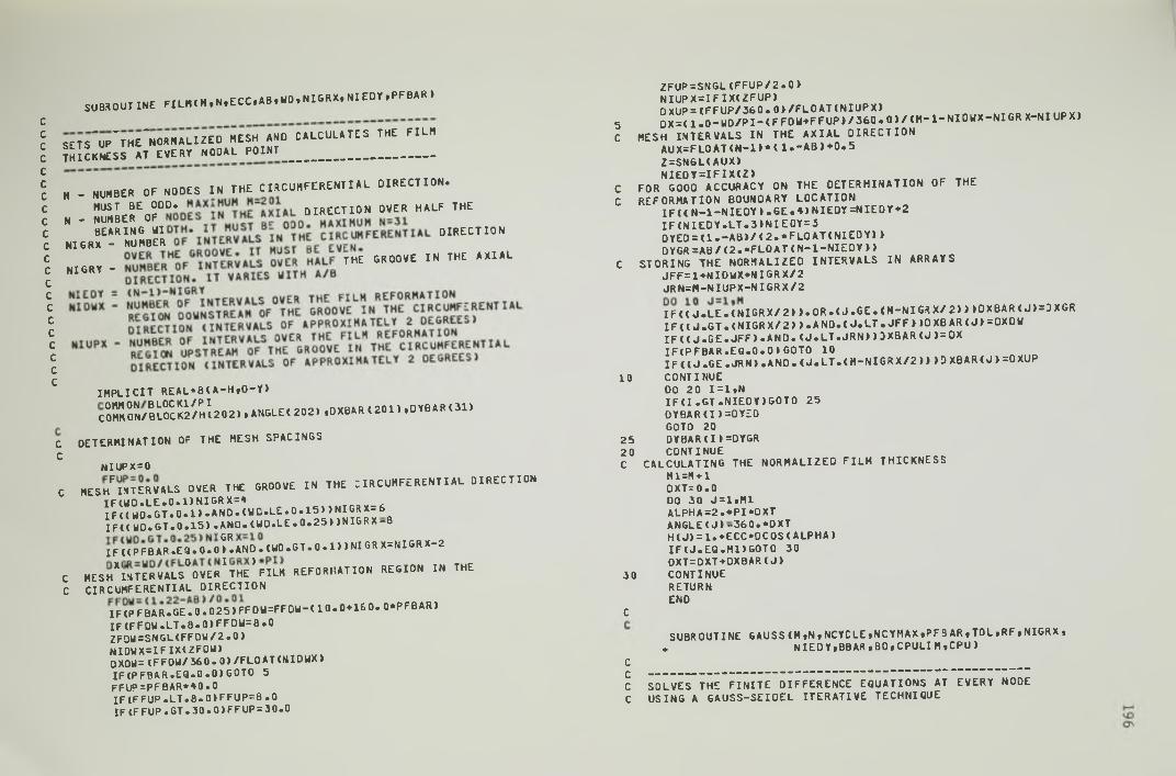
no
no
oo
on
no
on
oo
oo
no
oo
oo
SUBS OUTINE FILMCM»NtECC»ABtWDtNIGRX»NIEDY«PF8AR)
S£TS_UP_ THe "'n ORMALIZED MESH AND CALCULATES THE FILM THICKNESS AT EVERY NODAL POINT____________________________
„ - NUMBER OF NODES IN THE CIRCUMFERENTIAL D IRECTION .
MUST BE ODD. DIRECTION OVER HALF THE
I i’6rH ^ DIRECTI0N
— - ,HE “ M , E " ,HE ‘” ‘L
IM P LIC IT REAL*8(A-HtO -Y>
e S S / S t S S S ' c a o a * . angle ( 2021 .dxbar C201 > . d y b a r c s d
C DETERMINATION of th e HESH spacingsc
NIUPX=0
c MESH^INTERVALS OVER THE GROOVE IN THE CIRCUMFERENTIAL DIRECTION IFtt lD .LE .0 .1> N IG R X = 4 *«%*uTra*-fcI F {C U O .G T .0 .1 > .A N D .t U D .L E .0 .1 5 n N I G R X -6IF C t W D .G T .0 .1 5 » .A N O .t U D .L E .0 .2 5 )» N IG R X -8
IF CiPFBAR»EQ» O .O ^A N D • CU0»GT»0 • 1) )NI GR X=NIGRX-2
c HESH^MTERVALS^OVER^THE^ FILM REFORMATION REGION IN THE C CIRCUMFERENTIAL DIRECTION
IF<PFBAR«GE»0«025>FFDU=FFDU“ (1 0 «0*160« 0*PFBAR>IFCFFDU»LT«8«0)FFDU=8*0ZFDtl=SNGL(FFDU/2.0>NIDWX=IFIX(ZFOW>OXOU=IFFOU/360.Q>/FLOATCNIDUX>IFCPFBAR.EQ.O.OIGOTO 5 FFUP=PFBAR*40.0 IF C F F U P .L T .8 .0 )F F U P = 8 .0IF<FFUP.GT.30.0>FFUP=30.0
ZFUP=SNGL<FFUP/2.0>NIUPX=IFIXCZFUP>DXUP=CFFUP/360.0>/FLOATCNIUPX)
5 o x = (1 .0 -W D / P I -< F F O U * F F U P > / 3 6 0 .0 > / C M -l -N ID U X -N IG R X -N IU P X )
C MESH INTERVALS IN THE A XIAL DIRECTION A U X = F L O A T C N - l » * ( l . -A B > * 0 .5 Z=SN6L(AUX)N IED T= IFIX CZ> ___ _
C FOR GOOD ACCURACY ON THE DETERMINATION OF THE C REFORMATION BOUNDARY LOCATION
IF<< N - l - N I E D Y ) •GE»4>NIEDY=NIEDY+2 I F ( N I E D Y .L T .3 > N I E 0 Y = 3 D Y E D = ( 1 » -A B » / < 2 .» F L 0 A T < N I E D Y ) ) 0 Y G R = A B / (2 .* F L 0 A T (N -1 -N IE D Y > >
C STORING THE NORMALIZED INTERVALS IN ARRAYS JFF=l*NIDU X *N IGR X /2 JRN=M -NIUPX-NIGRX/2
I F C l J . L E « ( N I G R X / 2 > J . O R . < J . G E . ( M - N I G R X / 2 ) » >DXBAR<J)=3XGR I F < ( J . G T . C N I G R X / 2 ) ) . A N D . ( J . L T . J F F > >DXBAR<J)=DXDUI F ( C J . G E . J F F > . A N O . C J . L T . J R N ) » 3 X B A R ( J ) = D XIFC P F B A R .EQ .O .O )G O TO 10I F ( ( J . G E . J R N > . A N D . ( J . L T . < M - N I G R X / 2 » > D X B A R ( J > = 0 X U P
10 CONTINUEDO 20 I= 1 »N I F ( I . G T . N I E D Y ) G O T O 25 DYBAR(I>=OYEO GOTO 20
25 DYBARCI) =DYGR 20 CONTINUEC CALCULATING THE NORMALIZED F IL H THICKNESS
M1=M*1 DXT=0.0 DO 30 J=1«M1 ALPHA=2.*PI*0XT ANGLE («1 )-360* *DXT H ( J ) = 1 . * E C C *0COS(ALPHA>I F ( J . E Q . M l ) 6 O T 0 30 DXT=DXT-»DXBAR(J>
30 CONTINUE RETURN END
C
SUBROUTINE GAUSS CM ,N.NCYCLEtNCYMAX.PFBARtTOL»RF,NIGRX•♦ N I E D Y , 8 B A R , B O , CPULIM .CPU)
Cc — -----— ------------- -— ------ - — - “ “C SOLVES THE F I N I T E DIFFERENCE EQUATIONS AT EVERY NODE C USING A 6AUSS-SEIDEL ITER A TIV E TECHNIQUE

n o
o o
o o
C ------------------------------------------------------------------------------------------------------------C . „
IM P L IC IT R EA L*8(A -H tO -Z>
COMMON/BLOCK2/H(202> ,ANGLE(202»,DXBARt 201 j * ° T® * " <31> C0MM0N/BL0CK3/IG(32»2 0 2 ) »NG(32 t 2 0 2 ) » T P R E V ( 32*2 02 ) COHHON/BCOCKT/THETAC3 2 t202>
CTGR=1.«PFBAR/BBAR D B 2 = (1 ./B D »»* 2
GIVING I N I T I A L VALUES TO G AND THETA
NCYCLE=0CALL SETPAR(M.N»NCYCLE>
CALCULATING THETA AT EVERY NOOE POINT
10 IF(NCTCLE.GE.NCVMAX)GOTO 20DO 3 1=1tN DO 3 J=1»H
3 T P R E V t l i J » = T H E T A C I * J »DO I S I=2»N DO 15 J=2.M
C CHECKIN6 THE CPU TIME USED CPU=CPUTIM(X>IF (C P U .6 E .C P U LIM IG 0 T0 20
CIF ( I .N E .N > 6 0 T 0 4 TH ETAC N * 1 »J»= TH E TA (N -1 »J>
C BOUNDARY CONDITIONS AT THE GROOVE - PRESSURES ALL C ROUND THE GROOVE SET EQUAL TO THE SUPPLY PRESSURE« I F ( I . L E . N I E D Y » 6 0 T 0 5 ___ r
I F ( ( J . 6 T . ( 1 * N I G R X / 2 > I . A N D . C J . L T . (M -N IG R X / 2 )>IGOTO 5T H E TA C I» J)=TGR THETACI.1»=TGR
CGOTO IS
S IF (J .N E .M > 6 0 T 0 6T H E T A C I»M * 1 }= T H E T A (I•2)
b R G 1 = FL0 A T(N 6 (I•J ) )RG 2= F L O A T (N 6 ( I| J* 1 )>R63=FL0AT(N6( I ><1-1 ) )R64=FL0AT(N6(1*1» J))RG5=FL0AT(NG( 1 - 1 , J )>E 1 = (R 6 1 * H (J » * R 6 1 * R G 2 * t H (J * l ) -H C J ) )/ 2 . )E 2 = ((H < J * 1 ) -H < J> )* * 3 )* R G 2 * C T H E T A (I»J * 1 ) - l • >/DXBAR( J ) E 3 1 = T H E T A ( I » J -1 > » H (J -1 > * ( l . -R G 3 > '» R G 3 * H (J - l> E 3 2 = R 6 3 * R G l* (H (J » -H (J - l> > / 2 .E3=E31*E32
CO u
u u
E4=( ( H ( J ) + H ( J - 1 > > « * 3 > * R G 3 * ( T H E T A ( I t J _ l > “ 1 •*/ D X B A R (J - 1 >E 5 = ( H ( J > * * 3 ) * R G 5 * ( T H E T A ( I ” 1 » J > - 1 » J / D T B A R ( I “ HE 6 = ( H ( J ) #* 3 ) ,*RG4* C T H E T A (X * 1 . J » - 1 . » / D Y B A R C I >£ 7 1 = ( (H <J ) + H ( J - l ) ) * * 3 )* R G 1 / D X B A R (J - l )E72=( ( H ( J ) * H ( J * 1 ) > * * 3 ) * R G 1 / D X 8 A R ( J )E7=E71*E72 E 8 = H (J > * (1 « -R G 1 >E 9 1 = (H ( J ) * « 3 ) * R G 1 / D Y B A R ( I -1 >E 9 2 = (H ( J ) * * 3 ) » R G 1 / D Y B A R ( I JE9=E91*E92E10= E 3 -E1E11=E2*E4+E7E12=E3*E6*E9O X B = (D X B A R (J> * D X B A R (J - l> > / 2 .D Y B = (D Y B A R O > * 0 Y B A R (I~ l> > / 2 »T l l= ( PI *D XB* BBA R« DB2 *E1 2/ 24 .> '* DYB *E1 0/ 2«T12=DYB*BBAR*E11/(192.*PI>T21=(PI*D XB*BBAR *D B2*E9/24.»*D YB*E8/2. T22=DYB*BBAR*E7/(192» *PI>T N E W = (T1 1 * T 1 2 »/ (T2 1 * T 22)THETA ( I t J ) = T H E T A ( I . J> -*RF* ( T N E U - T H E T A ( I » J ) > IF (J*NE*M )GO TO IS THET A ( I « 1 ) = T H E T A ( I » M )
15 CONTINUEC BOUNDARY CONDITIONS AT THE BEARING EDGE
DO 8 J=1»MI F ( T H E T A ( 2« J ) . G E . l . J T H E T A ( 1 * J ) = 1 .I F ( T H E T A ( 2 t J > . L T . 1 . ) T H E T A ( 1 t J ) = T H E T A ( 2 , J )CONTINUE
RESETING THE VALUES OF G
NCYCLE=NCYCLE*1 CALL SETPAR(M»N»NCYCLE)DO 1 1 = 1 .N DO 1 J=1»MIF(NG(I,J).NE.IG(I,J))GOrO 10
1 CONTINUE DO 2 1 = 1 .N DO 2 J=1.MD IF = D A B S (T H E T A (I . J » - T P R E V ( I » J > > / T P R E V ( I t J > I F ( 0 I F . G E * T 0 L ) G 0 T 0 10
2 CONTINUE 20 RETURN
ENDCc
SUBROUTINE SETPAR(M»N»NCYCLE>

o o o o
o c r r c thf I N I T I A L VALUES OF 6 AND THETARESETS VALUES OF G AFTER A CYCLE» DEPENDING ON THET A.PREVIOUS 6 • S ARE RETAINED
COMMON/BLOCK 3 / I G <32*202)tNG< 3 2 12 02)»TPREV < 3 2 12 02) COMMON/BLOCK T / TH E TA (3 2 »2 0 2 )
CNI=N*1M l-M * lIF<N C YC LE.GT.O )GO TO 10 DO 1 I=1»N1 00 1 J=1»H1 N G ( 1 i J l - l
1 T H E T A C I » J ) = 1 «GOTO 20
10 DO 2 I = l t N l DO 2 J=1 .H 1 I G U t J ) = N G < I » J )IF C T H E T A < It J > • G E . l .> N G C I i J > = 1 I F < T H E T A < I » J ) . L T . l . ) N G < I » J ) = 0
2 CONTINUE 20 RETURN
ENDCC
SUBROUTINE PRESS<M»N»BBAR)C _ ________________________________
C CALCULATES THE NORMALIZED GAUGE PRESSURES AT EVERY NOOEC -------------------------------------------------------------------------------------------------------------------------- -C
IM P L IC IT REAL*8C A - H t O - Z )C0MM0N/BL0CK3/IG<32»2 02)»NG <32»202)tTPREV< 3 2 . 2 0 2 ) COMMON/BLOCKT/THETA<32.202)COMMON/BLOCM/P<3 1 .2 0 1 )
C00 1 1=1»N DO 1 J = l » «IF (N G (I i< J )«E Q «0 > G O TO 2 P < I , J ) = B B A R * < T H E T A < I » « i ) - l . >GOTO 1
2 P ( I . J ) = 0 .1 CONTINUE
RETURN END
C C
SUBROUTINE LOAD ( N>N>WBAR»ATTA)
C CALCULATES THE DIHENSIONLESS LOAD C A P A C ITY BY NUMERICAL C INTEGRATION OF THE PRESSURE D IS T R IB U T IO NC -------------------------------------------------------------------------------- --C
I M P L I C I T R E A L * 8 < A -H .O -Z )
COMMON/BLOCK2/HC202)•ANGLEC202)»DXBAR( 2 0 1 ) »DYBAR<31) COMMON/BLOCK*/P< 3 1 .2 0 1 )C0MM0N/BL0CK5/PFUN <201 )»A F U N < 2 0 1 )
CDO 10 I = 1 »N DO 15 J - l i MALPH A=2.*PI*AN GLE<«J)/360.P F U N < J )= -P < It J )* O C O S < ALPHA)
I S CONTINUEA F U N < I)= S IM P < P F U N .l .M «DXBAR)
10 CONTINUEP Y B A R = 2 . * P I * S I M P < A F U N » l t N » D Y B A R )DO 25 I = 1»N DO 30 J=1»MA LP H A = 2 .* P I* A N G L E < J)/ 3 6 0 .PFUN( J ) = P < I » J )* D S IN < A L P H A )
30 CONTINUEAFUN <I ) =SIMP<PFUN 11«MtDXBAR >
25 CONTINUEPXBAR=2«*PI*SIMP <AFUN . l .N »D Y B A R )ATTA = 18 0.*OATAN<PXBAR/PYBAR)/PI I F < A T T A .G E .O .O )G O T O 20 ATTA = 18 0 . 0+ATTA
20 gBAR=2.*DSQRT<PXBAR**2*PYBAR*»2)RETURNEND
CC
FUNCTION S IM P < F U N .K I.K .D B A R )C _ __________
C CALCULATES THE INTEGRAL OF A FUNCTION »F U N » USING C SIMPSON’ S RULE AND NON-EVEN MESH INTERVALS C -------------------------------------------------------------------------------------------------------------------------
C FUN - ARRAY H0L0IN6 THE VALUES OF THE FUNCTION TO BEC INTEGRATED _____c K I . K - NODAL POINTS DEFINING THE DOMAIN OF INTEGRATION C DBAR - ARRAY HOLOING THE MESH INTERVALS C
IM P L I C IT R E A L * 8 < A -H tO -Z )DIMENSION FUN <K > , DBAR<K)

oooo
oono
nnoo
nooo
oono
oooo
ooon
I F ( K I . E O . K » G O T O 20KK=K-1S IM P = 0 .0DO 10 I = K I .K K » 2A l= 2. *t D BA R< I> * »2 >A 2 = 3 . * 0 B A R ( I > * D B A R C I * 1 >A3=< DBAR< I *1 > # * 3*/DBARCI ) A 4 = 6 . » < D B A R ( I > ' » D B A R ( I * 1 > >A=( A1 *A 2- A3 )/A 4B1=2.*<DBARCI*1>**2>B2=(DBARCI)»*3>/0BAR<I*1>B = C 2 . * ( A 1 » A 2 * B H # A3+B2)/A4 C=CA2~B2*B1)/A4
10 SIMP=SIMP*A*FUN(I I*B*FUN<I*1»*C*FUNCI*2>
GOTO 30 20 SIMP=0.0 30 RETURN
END
SUBROUTINE C V R F (M .N .N IG R X .N IE D Y .P F B A R .J J . J C A V .J R .J R 1 •JR EF )
DETERMINES THE LOCATION OF THE CAVITATION AND THE REFORMATION BOUNDARIES
NIGRX - NUMBER OF MESH INTERVALS OVER THE GROOVE IN THE CIRCUMFERENTIAL DIRECTION
MIEDY - NUMBER OF MESH INTERVALS IN BETWEEN THE GROOVE AND THE EDGE OF THE BEARING
jCAV - CIRCUMFERENTIAL LOCATION OF THE POINT ON THE EDGE OF THE BEARING UHERE FILM RUPTURE OCCURS
JREF - CIRCUMFERENTIAL LOCATION OF THE POINT ON THE BEARING EDGE UHERE THE FULL WIDTH FILM BEGINS
J J - CIRCUMFERENTIAL LOCATION OF THE NOSE OF THE CAVITATION BOUNDARY
JR - CIRCUMFERENTIAL LOCATION OF THE NOSE OF THE REFORMATION BOUNOARY
j r 1 - CIRCUMFERENTIAL LOCATION OF THE NODE ON THEREFORMATION BOUNDARY* THE AXIAL LOCATION OF WHICHIS (N IED Y + 'l> _
NPREF1•NPREF2 - NUMBER OF POINTS ON EACH PORTION OF THE REFORMATION BOUNDARY WHEN SEPARATED INTO PARTS
X BCAV(K)•YBCAVtK) - ARRAYS HOLDING NORMALIZED COORDINATES OF POINTS ON THE CAVITATION BOUNDARY
X B R E F IK ). YBREFtK) - ARRAYS HOLDING NORMALIZED COORDINATES OF POINTS ON THE REFORMATION BOUNDARY
♦ XBREF1 ( 3 1 ) .YBREF1C31) » XB Ri F2 C61» t YBREF2C61»
CN1=N-1 YBAR = 0 . 0N IG S Y= C N - 1 ) “ NIE0Y NPREF1=NIEDY*1 NPREF2=2*NIGRY*1 DO 1 1 = 1 . N I F ( I . E Q . 1 ) G O T O 10 YBAR=YBAR*DYBARt1 - 1 )
C LOCATION OF THE C A V I T A T I O N BOUNDARY AND COORDINATES OF P OI NT S
C10 DO 2 J=2» N
I F < I T H E T A < I * J ) « L T » 1 » 0 ) . A N D . < T H E T A C l *J - D . E Q . 1 . 0 ) >6OT0 20
15 i F ( t T H E T A C I » J ) . L E . 1 . 0 » . A N D . < T H E T A < I » J - l > » G T . 1 . 0 ) > G O T O 20
2 CONTINUE20 I F ( I * E Q « N ) J J = J
I F ( I . E Q . 1 ) J C A V = J X B C A V ( I ) = A N G L E ( J ) / 3 6 0 .0 YBCAV(I )=YBAR
C LOCATION OF THE REFORMATION BOUNDARY ANO COORDINATES OF POINTS C
DO 3I F t l T H E T A t l .K —1 ) . L T . 1 . 0 ) . A N D . ( T H E T A < I » K ) « G E . 1 . 0 ) 1GOTO 30
3 CONTINUE30 XBREF( I>=AN6LECK)/360•0
YBREF <1 )=YBAR I F ( I . E Q . 1 » J R E F = K I F C I . E Q . < N I E 0 Y * 1 > » J R 1 = K I F C I . E Q . N ) J R = K
1 CONTINUE
C CALCULATION OF POINTS ON THE OTHER HALF OF THE CURVES C
DO 4 1 = 1 . N1XBCAV(N+I>=XBCAV < N - I )
4 Y BC A VC N* I )= 1 .0 -Y BC A V( N - I >DO 5 1 = 1 . N1X BR EF < N* I )= XB RE F( N- I )
5 Y B R E F ( N * I ) = 1 . 0 - Y B R E F < N - I »SO DO 6 I = 1.NPREF1
XBREF1CI)=XBREF < I )
C 0 M N 0 N / B L 0 C K 2 / H < 2 0 2 ) . A N G L E C 2 0 2 ) . D X B A R C 2 0 1 ) » D Y B A R C 3 1 )
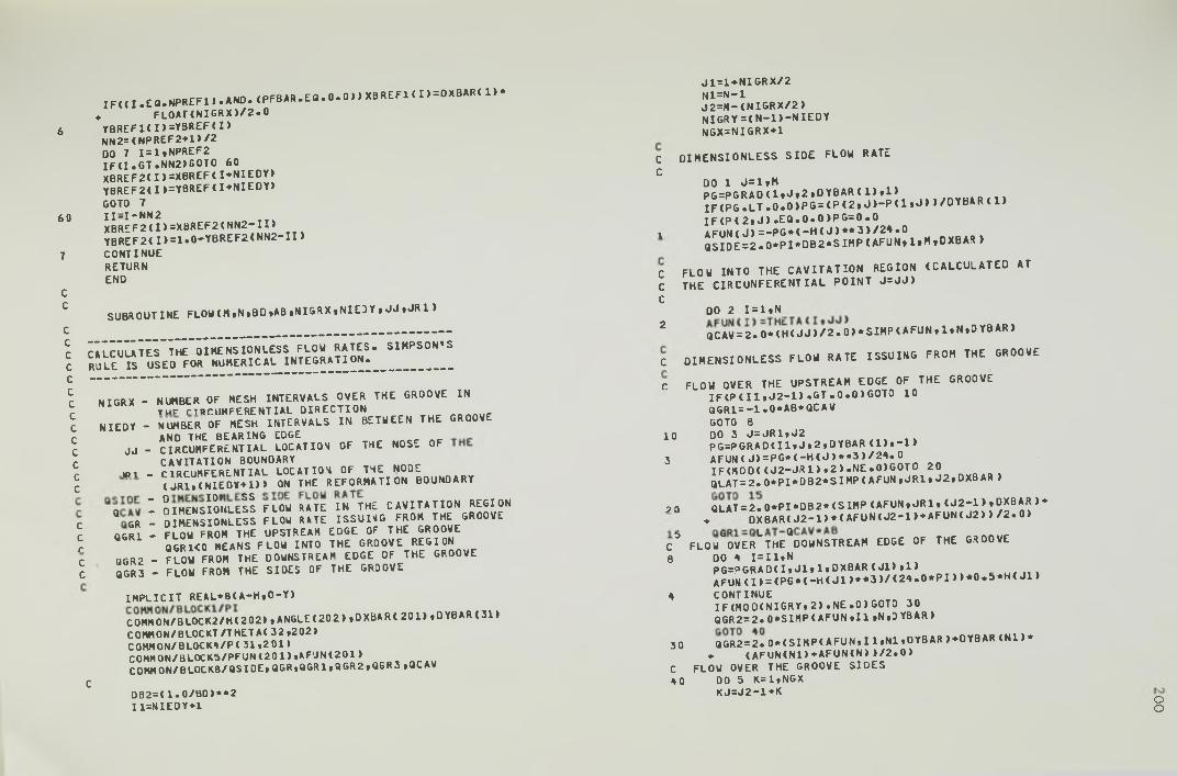
onon
ooon
nnoo
nnI F < t I .E O .N P R E F l» .A N D .< P F B A R .E Q .O .O )» X B R E F l (n = O X B A R < l )*
* FLOATCNI6RX) /2.06 VBREFK I ) = Y 9 R E F C I )
NN2=<NPREF2*l»/2DO 7 I=1.NPREF2 I F C I . G T . N N 2 I 6 0 T 0 60 XBREF2CI)=XBREFCI*NIEDY)YBREF2(I»=YBREFCI*NIEDY>GOTO 7
60 I I - I ~ N N 2X BR E F2 ( I» = X B R E F 2 ( N N 2 - I I »Y B R E F 2 C I ) = 1 . 0 - Y B R E F 2 ( N N 2 - I I )
7 CONTINUE RETURN END
C
C SUBROUTINE F L O U t M . N . B D . A B . N I G R X . N I E I Y t J J . J R 1 >
CALCULATES~ THE 01 HE NSION LESS FLOU RATES. SIMPSON'S RULE IS USED FOR NUMERICAL I N T EG RA TI O N .______________
NIGRX - NUMBER OF MESH INTERVALS OVER THE GROOVE IN t m f rTRCUMFERENTIAL DIRECTION
NIEDY - NUMBER OF MESH INTERVALS I N BETUEEN THE GROOVEa n d t h e b e a r i n g edge
J J - CIRCUMFERENTIAL LOCATION OF THE NOSE OF c a v i t a t i o n b o u n d a r y
i p i _ CIRCUMFERENTIAL l o c a t i o n o f t h e node( JR1» ( N I E D Y + 1 ) ) ON THE REFORMATION BOUNDARY
' S m i S u S FLOU U K I n ' t H E CA VI TA TI O N REGION C “ « : M K M M M * FLoU RATE ISSUING FROM THE GROOVE C QGR1 - FLOU FROM THE UPSTREAM EDGE OF THE GROOVE r QGR1<0 MEANS FLOU INTO THE GROOVE REGIONc QGR2 - FLOU FROM THE DOUNSTREAN EDGE OF THE GROOVE C OGR3 - FLOU FROM THE SIDES OF THE GROOVE
I M P LI C I T R E A L* 8 ( A- H « 0- Y )
COMMON/BLOCK2/H1202) »ANGLE<202> |DXBAR( 201) »DYBAR(31) COMM ON/BLOCKT /THETA( 32»202)COMMON/ BLOCK*/P t 31.201 > COHHON/BLOCK5/PFUNC201).AFUNl201)C0MM0N/BL0CK8/QSIDE»QGR»8GR1»BGR2»QGR3 »QCAV
CDB2=(I .0/B0>**2 I1=NIEDY»1
J1=1*NIGRX/2 N1=N-1J 2 = H -C N IG R X / 2 )N IG R Y = < N -1 ) -N IE D YNGX=NIGRX+1
C DIMENSIONLESS S ID E FLOU RATE C
00 1 J = 1 » NP G = P G R A D C l f J t 2 , D Y B A R < l ) t l )I F ( P G . L T . 0 . 0 ) P G = < P t 2 » J ) - P < 1 » J > )/ D Y B A R C l) I F C P < 2 » J ) * E Q . O . O ) P G = 0 . 0
1 A F U N < J ) = - P G * < - H < J ) * * 3 ) / 2 4 . 0Q S ID E = 2 .0 * P I* D B 2 * S IM P tA F U N tl»H tD X B A R )
C FLOU INTO THE C A V IT A T IO N REGION (C ALCULATED AT C THE CIRCUNFERENTIAL P O IN T J = J J )C
DO 2 I= 1 » N
2 aCAV= 2 . OMHC J J ) / 2 . 0 ) * S I M P ( A F U N t 1»N*D YBAR)
C DIMENSIONLESS FLOU RATE ISSUING FROM THE GROOVE
C FLOU OVER THE UPSTREAM EDGE OF THE GROOVE I F ( P ( I I *J 2 - 1 ) « G T . 0 . 0 ) GOTO 10aGRl=-1.0*AB*QCAVGOTO 8
10 DO 3 J = J R 1 » J 2P G = P G R A D ( I l » J » 2 » D Y B A R C l ) f - l )
3 A F U N tJ )= P G * C -H < J> * * 3 )/ 2 4 .0IF C H O D (<J 2 - J R 1 ) * 2 ) .N E .O )G O TO 20 Q LA T=2.0«P I*D B2*SIM P CA FUN »JR1 i J 2tDXBAR)
2 0 QLAT = 2.0*PI*DB2*CSIMP C A FUN tJR lt C J 2 -1 ) t D X B A R )♦♦ D X B A R C J2 -1 )*<AFUNCJ2” 1 )* A F U N C J 2 ) ) / 2 . 0 )
C5 FLOUGOVERL THEflDOUNSTREAM EDGE OF THE GROOVE6 DO 4 I = I 1 » N
P G = P G R A D ( I » J l i l » D X B A R ( J l ) » 1 > # .AFUN C I ) = ( P G * < - H < J 1 ) * * 3 ) / < 2 4 . 0 * P I ) ) * 0 . 5 * H < J 1 )
4 CONTINUEIFC M O D (N IG R Y t2 ).N E .O )G O TO 30 QGR2S 2.0*SIHP<AFUN t i l »N»0 YBAR)
30 Q G R 2 =2.0*C SIM P <AFU N .IlfN ltD YBA R)*D YBA RC N l)*♦ (A F U N < N 1 )+ A F U N C N ))/ 2 .0 )
C FLOU OVER THE GROOVE SIDES 40 00 5 K=ltNGX
K J= J2 -1 * K o o

nn
oo
oo
oo
oo
oo
no
oo
oo
oo
o
n
IF C K J .G E .M )K J= K J -M * 1P G = P G R A 0 t I l t K J t 2 » D Y B A R ( l ) « - l>
5 A F U M C K J » = P G * < - H C K J » * * 3 > / 2 4 . 0
AFUN(H»=AfrUN(l)IFCKOD<<M-J2)i2>.NE.O>GOTO 6
S 1= S IM P <AFUN,J2,M ,DXBAR>
S 2 = S IM P < A F U N .ltJ l»0 X B A R )
6 S1=SIMP CAFUNtJ2.(M-l)»0XBAR)*DXBAR<1-11*<AFUNCH-1>+AFUN(H) )/2«S2=SIMP CAFUNt 1 • < J 1 -1 ) fDXBAiD+
♦ D X B A R C J 1 - 1 > * C A F U N C J l - l ) ^ A F t W C J l ) ) / 2 * 07 QGR3=2«0*PI*DB2*CS1*S2)c TOTAL NET FLOW ISSUING FROM THE GROOVE
QGR=QGR1+QGR2*QGR3 RETURN ENO
FUNCTION PG RAD(IGtJGiKFL0U«S6R ID»K6)
CALCULATES THE PRESSURE GRADIENT AT A NODAL POINT
I T I S ASSUMED THAT THE VARIATION OF PRESSURE IN THE NEIGBOURHOOO OF A NODAL POINT CAN BE REPRESENTED BY A POLYNOMIAL OF DEGREE 3 .
I G . J G - GRID LOCATION OF THE NODE WHERE THE PRESSURE GRADIENT IS REQUIRED
KFLOU - INDICATOR* KFLOH=l I F I T IS REQUIREO THE FLOU THROUGH A SECTION OF CONSTANT X KFL0W=2 I F I T I S REQUIRED THE FLOU THROUGH A SECTION OF CONSTANT Y
SGRID - S IZE OF MESH INTERVALS INVOLVED IN THE CALCULATIONSKG - I S GIVEN THE VALUE 1 OR - 1 DEPENDING ON UHAT
OIRECTION IS BEING TAKEN TO CALCULATE THE PRESSURl GRADIENT
IM P L IC IT R E A L*8(A -H t 0 - Y )COHN0N/BL0CK4/P( 31*201)
C .I F <KFL0U<EQ<21GOTO 10PGRAD=(-11«0*P< IG » JG)*18» 0 »P < IG , JG+KG) - 9 . 0*P <IG» 2*KG*JG) ♦
♦ 2 .0 * P < IG » 3*KG*JG) )/(6.0*SGRID>GOTO 20
10 P G R A D = l -1 1 .0 * P (IG »JG )* 1 8 .0 »P ( IG * K G * JG ) - 9 . 0* P (2 * K G * IG tJG )♦♦ 2»0*P( 3 «K G*IG »JG) )/ (6 .0 * S G R I0 )
20 RETURNEND
on
no
n
n o
oo
on
oo
oo
oo
o
n
SUBROUTINE DIAG< M » N « N I G R X » N I E D Y » J J » J C A V •JR »«JR 1»JREF*B D .♦ E C C »A B »U O »P F B A R »IG R ID )
DRAUS THE CA V ITA TIO N AND THE REFORMATION BOUNDARIES AND THE MESH REPRESENTATION ( I F REQUIRED)
THE CALL TO DEVICE NOMINATION AND THE CALL TO ‘ DEVEND UERE HADE IN THE MAIN PROGRAM TO ALL0U FOR MORE THAN ONE GRAPH TO BE STORED IN THE SAME PLOT F I L E
IM P L I C I T R E A L * 8 C A -H tO -Y ) ___C0MM0N/BL0CK2/HC2 0 2 ) » ANGLE< 2 0 2 ) »DXBAR<2 0 1 ) iDYBAR(3 1 ) C0MM0N/BL0CK7/XBCAVC61)tYBCAV< 6 1 ) » X B R E F C 6 1 )» YBR EF(6 1 )•
♦ XBREF1( 3 1 ) , YBREF1C31) »XBREF2( 6 1 ) • Y BR EF2(61)COMMON/BLOCKZ/ZXCUR<3)tZYCUR(3)
N I= N IE 0 Y + l JG = M -(N IG R X / 2 )
CALL PICCLECALL P E N S E L ( l t O . 0 » 0 )
DRAUING THE MESH OVER HALF THE BEARING AREA XL*YU ARE THE SIDES OF A RECTANGLE REPRESENTING THE BEARIN6 AREA
XL=140.0 YU=S0 *0DXGR=FLOAT«NIGRX)*DXBAR<l)DYGR=FL0AT( 2 * ( N - 1 - N I E D Y ) ) * D Y B A R ( N - l )XG=0.5-DXGR/2.0 YG=FL0AT CNIEDY)*DYBAR( 1 )
DO 100 I =l » 2I F C C I . E Q . D . A N D . C IG R I 0 .E Q .0 ) ) GOTO 10 0 DX=120.0D Y= 1 95 .O -FLO A T( 1 - 1 )*8 0.0CALL T R A N S F ( - l )CALL S H IF T 2 (D X ,D Y )CALL MOVT02<0.0 , 0 . 0 )CALL L IN B Y 2 < 0 .0 tY U )CALL L I N B Y 2 ( X L , 0 . 0 )CALL L IN B Y 2 (0*0 t —YU)CALL L I N B Y 2 ( -X L t O . O )CALL S C A LE2 (X LiY U )
DRAUING THE GROOVE 201

CALL HOVTO2C0.5 * 0 . 0 )CALL SYMB0LC3)CALL M0VT02CXG.YG)C A U LINBY2C0.0*DYGR)CALL LINBY2CDXGR * 0 . 0 )CALL L I N BY 2 C0 . 0* - DY G R)C A U L I NBY 2 C- DX GR» 0 .0 )I F ( I •E Q . 2 ) 0 0 1 0 100
C DRAUING THE AXIAL MESH LINES DO 200 JGR=2*M XM=ANGLECJGR)/360. 0 I F C X N . L T . 0 . 5 ) G 0 T 0 70 XH=XN-0.5 GOTO 80
70 XM=XM*0. 5 80 CALL HOVTO2CXM.0.0)200 CALL L I N B Y 2 C 0 . 0 * 0 . 5 )C DRAUING THE CIRCUMFERENTIAL NESH LINES
YM=0.0DO 300 IGR=2*N YM=YB*DYBARCIGR-1)CALL MOVT02C 0•0 » Y H)
300 CALL L I N B Y 2 C 1 . 0 * 0 . 0 )100 CONTINUE CC DRAUING THE CA VI TA TI O N BOUNDARY C - THREE POINTS ONLY - C
00 1 1=1*3 I I = I * C I - l ) * C N - 2 )ZXCUR(I )=SNGLCX8CAVC1 1 > > -0 .5 ZYCUR(I )=SNGLC Y B C A V C I I ) )
I CONTINUECALL CURT02C ZXCUR•ZYCURt3 *0*0)CALL C H A S I Z C 2 . 0 * 2 . 5 )CALL MOVT02CCZXCURC2)* 2 . 0 / X L ) * CZYCURC2) *1.0/YU) ) CALL CHAH0LC13HCAVITATI0N * . )CALL CHAH0LC8HREGI0N*•)CALL HOVT02( (ZXCUR( 2 ) * 2 . 0 /XL) iCZYCUR< 2 ) - 3 . 0 /YU) ) CALL CHAH0L(8HEDGE * . )CALL CHAFIX<ANGLECJCAV)*7,1)CALL CHAH0LC6H D EG *. )CALL M0VT02<( Z X C U R ( 2 ) + 2 . 0 / X L ) • ( ZYCUR< 2 ) - 7 « 0 / Y U ) ) CALL CHAH0L(8HN0SE * . )CALL C H A F I X ( A N G L E C J J ) t 7 » l >CALL CHAH0L(6H O EG * . )
CC DRAUING THE REFORMATION BOUNDARYC
IF( P FB AR .E Q. O .O )G OT O 10
in cm
uo
u
I F < < J R E F . L E . J G ) . A N D . ( < XBREF( 1 ) * 0 . 5 ) . G T . 1 * 0 ) ) GOTO 60 I F < ( J R 1 - J R ) . G E . 2 ) G 0 T 0 60
10 A U X = F L 0 A T ( N I ) / 2 . 0 Z=SNGL<AUX)N P = I F I X < Z ) * l DO 3 1 - 1 * 3 I I = I * « I - l » * < N P - 2 )I F ( ( I . E Q . 3 ) . A N D . ( M O D <N I * 2 ) . E Q . 0 ) ) 1 1 = I I - 1 ZXCUR<I)= S N G L C X B R E F 1 (I I> >ZYCUR 11 ) = S N G L < Y B R E F 1 C I D )I F ( Z X C U R C I ) » G E . 0 . 5 ) G O T O 30 ZXCUR( I ) =ZXCUR C l ) + 0 . 5 GOTO 3
30 Z X C U R ( I ) = Z X C U R ( I > - 0 » 53 CONTINUE
CALL CURT02<ZXCUR*ZYCUR*3*0*0)C
DO 4 1=1*34 ZYCUR C l ) = 1 . 0 - Z Y C U R ( I )
CALL CURT02CZXCUR.ZYCUR,3 . 0 * 0 )I F C P F 8 A R . E a . O . O ) G O T O 20
CNP=N-NI£OY DO 5 1=1*3 I I = I * C I - l ) * C N P - 2 )ZXCUR C l ) = S N G L C X B R E F 2 C I I ) ) - 0 . 5 Z Y C U R C l ) = S N G L ( Y B R E F 2 ( I I ) ) •
5 CONTINUECALL CURT02CZXCUR *ZYCUR* 3*0* 0)GOTO 20
C60 DO 2 1=1*311=1♦CI — 1)*CN~2)
ZXCUR C I >=SNGL CXBREF C11) )ZYCURCI) =SNGLC YBREFC11) )I F C Z X C U R C D . G E . 0 . 5 ) GOTO 50 ZXCUR C I ) =ZXCURCI) ♦ 0 . 5 GOTO 2
0 ZXCURCI ) =ZXCURCI> - 0 . 5 CONTINUECALL CURT02CZXCUR* ZYCUR*3*0. 0)
UK I T I NG STRIN6S OF CHARACTERS
20 CALL M0VT02CCDXGR/2.0 * 0 . 5 * 5 . 0 / X L ) * C 0 . 5 * 1 . 0 / Y U ) )CALL CHAH0LC18HFULL FIUM REGI ON*. )CALL M0VT02CCDXGR/2.0 * 0 . 5 * 5 . 0 / X L ) » C 0 . 5 - 3 . 0 / Y U ) )CALL CHAH0LC7HEDGE * . )CALL CHAFIXCANGLECJREF)*7*1)CALL CHAH0LC6H OEG *. ) 202
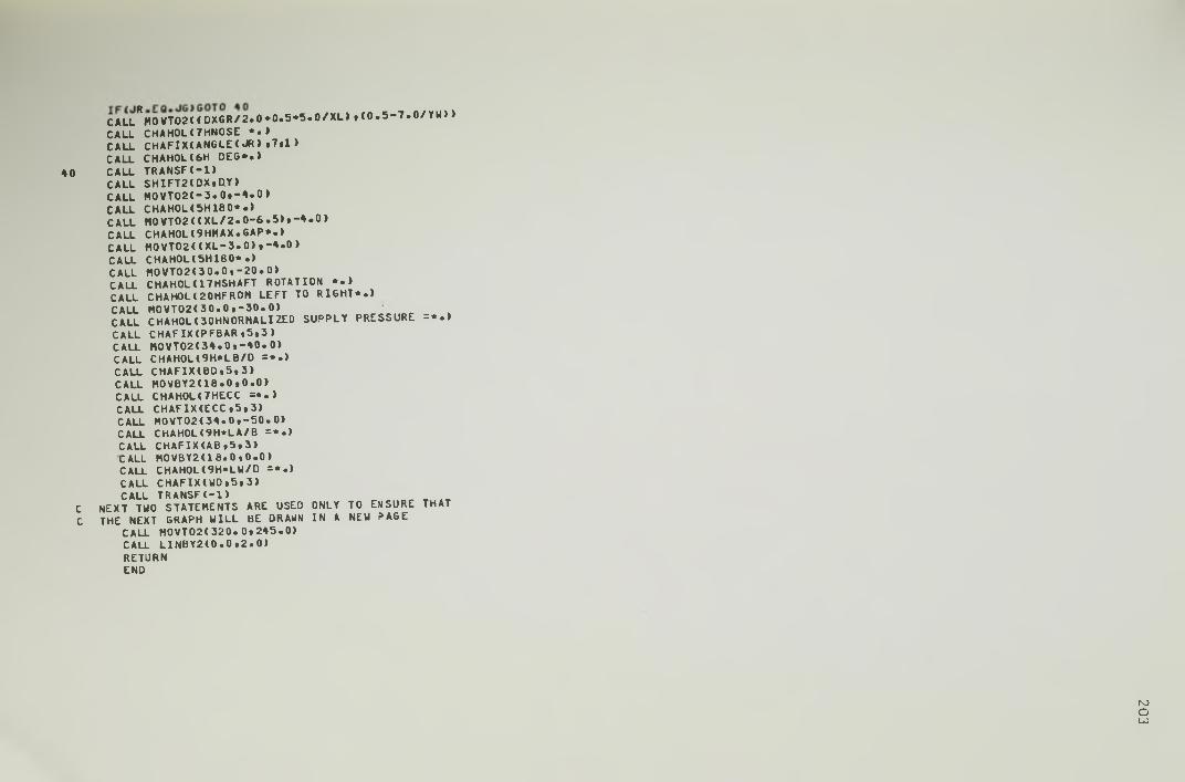
C A L L R H O W T 0 2 t C D X G R / 2 . 0 * 0 . 5 * 5 . 0 / X L » t < 0 . 5 - 7 . 0 / Y U ) ) CALL CHAH0L<7HN0SE ••>C A U CHAFIXCANGLE< JR> »7»1 )CALL CHAH0L(6H DEG*.»
40 CALL T R A N S F ( - l )CALL SHIFT2CDX.ttY>CALL M O V T 0 2 < - 3 . 0 t - 4 . 0 »CALL CHAHOL<5H1BO«. )CALL M O V T 0 2 < t X L / 2 . 0 - 6 . 5 ) ( - 4 . 0 )C A U CHAH0LC9HMAX.GAP*.)CALL M O V T 0 2 ( ( X L - 3 . 0 ) t - 4 . 0 )C A U CHAHOLC5H180* . )CALL MOWT02<30.0» -20.0>C A U CHAHOLC17HSHAFT ROTATION * . )C A U CHA HO H2 OHFROH LEFT TO R I G H T * . >CALL MOVT 02 <3 0. 0( - 3 0 . 0 1CALL CHAHOLtSOHNORHALIZEO SUPPLY PRESSURE = * . ) CALL CHAFIX(PFBAR( 5 ( 3 )CALL M O V T 0 2 ( 3 4 . 0 * - 4 0 . 0 )CALL CHAH0L(9H*LB/D = * . )C A U C H AF I X( B D( S ( 3 >CALL H 0V B Y 2 ( 1 8 . 0 ( 0 . 0 )C A U CHAH0H7HECC = * . )C A U C H A F I X( E C C( 5 ( 3 >C A U M0VTO2C34.0 ( —5 0 . 0 )C A U CHAH0L(9H*LA/B = * . )C A U C HA F I X C A B ( 5 ( 3)CALL HOWBY2C18.0(0.0)C A U CHAH0LC9H*LU/D = * . )C A U C H A F I X ( U 0 ( 5 ( 3 )CALL TRANSF( - 1 )
C NEXT TWO STATEMENTS ARE USED ONLY TO ENSURE THAT C THE NEXT GRAPH U I L L BE ORAHN I N A NEW PAGE
C A U H0VT02C 320. 0 ( 2 4 5 . 0 )C A U L I N B Y 2 « 0 . 0 ( 2 . 0 )RETURNEND
N>oLO

204
APPENDIX C BEARING PERFORMANCE PREDICTIONS
The performance predictions shown in the table that follows
apply to journal bearings with a single oil groove at the maximum
film thickness and a/b = 0 . 8 and w/d =0.2.
In a few cases, marked (*) in the table, convergence of the
Gauss-Seidel iteration was not achieved. The results shown for
these cases have been obtained for w/d = 0.19.
The following sketch of the developed bearing area serves to
identify some of the parameters involved.
205
\b a ar cPf b/d e W I (deg)
J.(deg) (deg)
0.0 0.5 0.2 0.154 0.151 0.404 72.1 49.5 193.70.4 0.405 0.301 0.307 60.0 47.5 193.70.6 1.001 0.449 0.209 47.1 47.5 193.70.8 3.497 0.602 0.108 32.5 45.5 193.7
0.6 0.2 0.214 0.146 0.405 70.1 49.5 194.00.4 0.553 0.291 0.309 60.1 47.5 194.00.6 1.332 0.435 0.211 47.5 47.5 194.00.8 4.374 0.577 0.110 33.2 45.5 189.3
0.7 0.2 0.278 0.141 0.407 71.4 49.5 198.7
0.4 0.712 0.279 0.311 60.1 47.5 198.7
0.6 1.665 0.417 0.213 48.0 45.5 194.0
0.8 5.188 0.553 0.111 33.8 45.5 194.0
0.8 0.2 0.346 0.135 0.408 70.9 49.5 198.7
0.4 0.875 0.267 0.314 60.1 47.5 198.7
0.6 1.997 0.397 0.216 48.3 45.5 194.0
0.8 5.927 0.525 0.112 34.4 43.5 194.0
0.9 0.2 0.416 0.129 0.410 70.5 49.5 198.7
0.4 1.041 0.255 0.316 60.1 47.5 198.7
0. 6 2.320 0.376 0.218 48.6 45.5 194.0
0.8 6.597 0.495 0.113 34.9 43.5 194.0
1.0 0.20.40.60.8
0.487 1.205 2.624
1 7.199
0.1240.2420.3560.465
0.4120.3180.2200.114
70.160.049.035.3
49.547.545.543.5
203.4198.6193.7193.7
206
f o apf b/d e W I Q c (deg)
r(deg)
c(deg)
0.25 0.5 0.2 0.213 0.609 0.404 123.7 344.5 194.30.4 0.386 1.022 0.307 84.5 346.5 194.30.6 0.926 1.518 0.209 56.3 346.5 194.30.8 3.390 2.119 0.108 34.4 344.5 189.9
0.6 0.2 0.267 0.484 0.405 113.9 344.5 194.30.4 0.536 0.816 0.309 79.2 346.5 194.30.6 1.261 1.211 0.211 55.0 346.5 194.30.8 4.252 1.686 0.111 35.2 346.5 189.9
0.7 0.2 0.330 0.405 0.407 106.5 344.5 198.70.4 0.700 0.692 0.311 75.7 346.5 194.30.6 1.603 1.025 0.213 54.5 346.5 194.30.8 5.069 1.414 0.111 35.7 346.5 189.9
0.8 0.2 0.400 0.348 0.408 100.9 346.5 198.7
0.4 0.872 0.599 0.314 73.5 348.5 198.7
0.6 1.946 0.885 0.216 54.2 348.5 194.3
0.8 5.821 1.214 0.112 36.2 346.5 194.3
0.9 0.2 0.474 0.304 0.410 96.6 346.5 198.7
0.4 1.047 0.531 0.316 71.8 348.5 198.7
0.6 2.281 0.783 0.218 54.0 348.5 194.3
0.8 6.504 1.060 0.113 36.7 348.5 189.9
1.0 0.2 0.551 0.274 0.412 93.3 346.5 203.0
0.4 1.222 0.476 0.318 70.6 348.5 198.7
0.6 2.599 0.697 0.219 54.0 351.4 194.3
0.8 7.118 0.946 0.114 37.1 348.5 189.9

207
^ a aPf b/d £ W I Qc (deg)
r(deg)
c(deg)
0.5 0.5 0.2 0.363 1.099 0.404 147.3 338.5 196.70.4 0.434 1.775 0.307 109.6 340.5 192.20.6 0.863 2.642 0.209 67.4 340.5 192.20.8 3.241 3.702 0.108 36.9 340.5 192.2
0.6 0.2 0.410 0.845 0.405 138.4 338.5 196.70.4 0.569 1.378 0.309 99.2 340.5 196.70.6 1.196 2.043 0.211 63.8 340.5 192.20.8 4.132 2.858 0.111 37.1 340.5 192.2
0.7 0.2 0.466 0.683 0.407 130.3 338.5 196.70.4 0.727 1.121 0.311 92.3 340.5 196.70.6 1.544 1.659 0.213 61.7 340.5 196.70.8 4.963 2.311 0.111 37.5 340.5 192.2
0.8 0.2 0.529 0.574 0.408 123.4 338.5 201.30.4 0.898 0.943 0.314 87.4 340.5 196.70.6 1.893 1.390 0.216 60.6 342.5 196.7
(*)0.8 5.728 1.898 0.112 37.9 341.1 192.2
0.9 0.2 0.598 0.493 0.410 117.4 338.5 201.3
0.4 1.076 0.811 0.310 83.9 342.5 196.7
0.6 2.237 1.190 0.218 59.7 342.5 196.7
0.8 6.382 1.650 0.113 38.6 342.5 192.2
1.0 0.2 0.672 0.431 0.412 112.4 338.5 201.3
0.4 1.256 0.708 0.319 81.2 342.5 196.7
0.6 2.571 1.045 0.220 59.1 342.5 196.7
0.8 7.005 1.429 0.114 39.0 342.5 192.2

208
ip a aif b/d e W (deg)
L(deg) (deg)
1.0 0.5 0.2 0.736 2.127 0.404 162.6 328.5 195.10.4 0.696 3.369 0.307 140.6 332.5 195.10.6 0.836 4.993 0.209 94.3 332.5 195.10.8 2.972 7.047 0.108 41.9 332.5 190.4
0.6 0.2 0.796 1.610 0.405 157.2 328.5 195.10.4 0.799 2.555 0.309 129.9 332.5 195.10.6 1.137 3.780 0.211 84.5 332.5 195.10.8 3.851 5.314 0.110 41.6 332.5 190.4
0.7 0.2 0.856 1.282 0.407 151.6 328.5 199.9
0.4 0.928 2.033 0.312 120.5 332.5 195.1
0.6 1.473 3.006 0.213 78.8 332.5 195.1
(*) 0.8 4.685 4.126 0.111 41.6 333.1 190.4
0.8 0.20.40.60.8
0.9181.0791.8255.434
1.0571.6772.4733.455
0.4090.3140.2160.112
146.2112.874.942.1
326.5332.5332.5332.5
199.9195.1195.1 190.4
0.9 0.2 0.4 0.6
(*)0.8
0.9831.2452.1816.163
0.8951.4192.0872.854
0.4100.3170.2180.113
141.1106.672.342.3
326.5332.5332.5 333.1
199.9199.9 195.1 190.4
1.0 0.2(*)0.4
0.60.8
1.0501.4172.5296.803
0.7721.1971.7942.491
0.4120.3190.2210.114
136.3101.4 70.4 42.7
326.5 332.8332.5332.5
199.9199.9195.1195.1