offshore technology report 2000/130
TRANSCRIPT

HSEHealth & Safety
Executive
Examination of the effect of relief deviceopening times on the
transient pressures developed withinliquid filled shells
Prepared by the University of Sheffield
for the Health and Safety Executive
OFFSHORE TECHNOLOGY REPORT
2000/130

Examination of the effect of relief deviceopening times on the
transient pressures developed withinliquid filled shells
B C R Ewan, D Nelson and P Dawson
Department of Chemical and Process EngineeringUniversity of Sheffield
Mappin StreetSheffield
S1 3JD
HSE BOOKS
HSEHealth & Safety
Executive

© Crown copyright 2001Applications for reproduction should be made in writing to:Copyright Unit, Her Majesty’s Stationery Office,St Clements House, 2-16 Colegate, Norwich NR3 1BQ
First published 2001
ISBN 0 7176 1985 0
All rights reserved. No part of this publication may bereproduced, stored in a retrieval system, or transmittedin any form or by any means (electronic, mechanical,photocopying, recording or otherwise) without the priorwritten permission of the copyright owner.
This report is made available by the Health and SafetyExecutive as part of a series of reports of work which hasbeen supported by funds provided by the Executive.Neither the Executive, nor the contractors concernedassume any liability for the reports nor do theynecessarily reflect the views or policy of the Executive.

SUMMARY
A recent Joint Industry Project under the management of the Institute of Petroleum has beenconcerned with the failure scenario in which a shell and tube heat exchanger with a lowpressure rated shell and with a high pressure tube-side suffers tube failure.For water filled shells, the ensuing scenario is one in which a gas bubble rapidly growsaround the burst site generating a rising pressure wave within the shell. This pressure wave iseventually relieved when the protective hardware operates leaving a residual lower pressuretail as the water is driven out of the shell.Tube failure for a shell protected by a relief device therefore gives rise to a transient pressurepulse whose characteristics are influenced by the failure site geometry and location and thelocations and dimensions of the relief points.The study revealed the importance of relief device opening times on the peak pressures whichcould result and the present work being reported has been concerned with providinginformation on such opening times for a range of devices including bursting discs and reliefvalves.The experimental work has been performed at University of Sheffield and the data from thishas been subjected to a hydraulic modelling analysis by PSI Ltd providing a good overview tothe sequence of events associated with wave propagation and relief operation.Opening can be defined in a number of ways ranging from the instant at which pressurebegins to be relieved to the time at which the relief device is fully open. Ultimately, devicesmust be chosen which meet the relief requirement on a timescale which is compatible with theupstream system design and its failure characteristics. This represents an issue of sizing aswell as relief design choice.The devices studied have not been chosen to meet any particular relief objective, and itbecame clear that the bursting discs were oversized for the relief duty whilst the relief valveswere undersized. However, the data acquired enabled the times to full opening to be measuredwith a high degree of confidence.
The burst discs ruptured in 1.9-10 msec and this is in line with (and therefore supportive of)the values used in the IP study, which formed the basis of the IP Guidelines.The study also shows that the pop-action of the relief valves (RVs) studied occurred in 2.5-4msec but this finding, in particular, should be viewed with extreme caution and should not betaken out of context. We believe it would be premature if these values were taken as typicaland applied across the industry in general, for all sizes of device and all operating conditions.Overall, our reservations are as follows:Firstly, the study implies that RVs are faster than a metal burst disc but this, potentiallymisleading finding, has arisen by comparing a vastly oversized (8") disc against a severelyundersized, (2in) RV.Secondly, the study has given the unexpected finding of very fast opening times for the RVs,(4msec) almost 100 times faster than some of the values quoted by others. Although a quickresponse can be expected from the test case (the valve is very small and it is the pop-actiontype) this may not be typical in the field
ii

iii
CONTENTS
page
SUMMARY ii
1. BACKGROUND AND OBJECTIVES 1
2. PLAN OF WORK 2
3. METHODOLOGY 2
3.1 Test Details 2
3.2 Test Characteristics 4
3.3 Experimental facilities 5
3.4 Experimental Method 7
4. RESULTS 8
4.1 Pressure Traces 8
4.2 Video Tape 8
5. ANALYSIS 9
5.1 Summary of modelling analysis 95.2 Preliminary Appraisal 145.3 Open Tube Tests 175.4 Graphite Burst Disc Tests 205.5 Stainless Steel Burst Disc Tests 265.6 Spring Loaded RV, High Pressure Test 315.7 Spring Loaded RV, Low Pressure Test 355.8 Pilot Operated relief Valve Test 39
6. CONCLUSIONS AND RECOMMENDATIONS 43
7. APPENDIX 45
7.1 Plates 457.2 Data Charts 557.3 Video tape record 73

1. BACKGROUND AND OBJECTIVES
A recent Joint Industry Project under the management of the Institute of Petroleum has beenconcerned with the failure scenario in which a shell and tube heat exchanger with a low pressurerated shell and with a high pressure tube-side suffers tube failure.For water filled shells, the ensuing scenario is one in which a gas bubble rapidly grows aroundthe burst site generating a rising pressure wave within the shell. This pressure wave is eventuallyrelieved when the protective hardware operates leaving a residual lower pressure tail as thewater is driven out of the shell.Tube failure for a shell protected by a relief device therefore gives rise to a transient pressurepulse whose characteristics are influenced by the failure site geometry and location and thelocations and dimensions of the relief points.The experimental study indicated that pulse widths could be in the range 1 - 10 msec for thegraphite bursting discs used, and this was comparable to results from recent numerical work byCassata et al1 for a longer shell, where pulse widths in the range4 - 20 msec could be obtained with amplitudes of up to 25% of the tube-side pressure.
A recent parallel study2 was concerned with the response of the shell structure within the timeduration of the pulse loading, and concluded that engineering benefits could be secured byensuring the pulse widths were kept as short as possible compared with the fundamental periodof the shell structure. In this case, peak pressure amplitudes several times the yield pressure ofthe shell could be tolerated. Since shells will typically have fundamental periods in the range 5 -20 msec, design efforts should be directed at limiting pulse widths to 1/2 - 1/3 of this range. Thechoice of relief device is important in this context as well as the number of such devices andtheir distribution on the shell.
The objective of the work now being reported has been to measure a number of relief deviceopening times and to consider their effect on the amplitude and duration of transient vesselpressures arising from high pressure tube failures. This has been carried out through a series ofcontrolled experiments to monitor transient pressures in a water filled column combined with ahydraulic analysis of the dynamic event.
1

2
2. PLAN OF WORK
The programme of work undertaken had the following specific objectives :
1. To measure the opening times of a range of pressure relief devices when subjected to rapidlyrising pressure within a water medium,
2. To monitor the rates of pressure rise and peak pressures in the water column, which resultfrom chosen combinations of gas discharge pressure and orifice size,
3. To provide an interpretation of the key features of the pressure behaviour using current understanding of transient hydraulics.
3. METHODOLOGY
The shock tube schematic shown in Figure 3.1 and described in greater detail below, was usedfor the experiments.
bursting diaphragmand orifice location
high pressuredriver section
reliefdevice
9 m3 m
water filleddriven section
+ + + + ++
+ = pressure transducer
21
Figure 3.1 Outline of shock tube used for experiments
This is instrumented with a number of Kistler pressure transducers along its length.
The shock tube has a 100mm internal diameter and transition sections were available to extendthis to 200mm. It was intended that relief devices be examined whose diameters arerepresentative of those used offshore and that these should cover a range of types from thefastest to the slowest operating and include bursting discs, spring loaded and pilot operated reliefvalves.
3.1 TEST DETAILS
Since the key features of the effect of relief device opening time could be demonstrated over awide range of pressures, it was proposed that tests be carried out with relief devices whichoperate at a nominal 15 bar gauge pressure. The shock tube gas driver pressure was set at 100

3
bar and pressurisation of the water column locating the relief device was by means of rapiddischarge through suitably sized orifices.
4
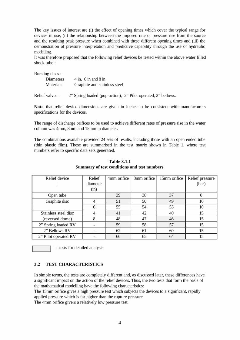
The key issues of interest are (i) the effect of opening times which cover the typical range fordevices in use, (ii) the relationship between the imposed rate of pressure rise from the sourceand the resulting peak pressure when combined with these different opening times and (iii) thedemonstration of pressure interpretation and predictive capability through the use of hydraulicmodelling.It was therefore proposed that the following relief devices be tested within the above water filledshock tube :
Bursting discs :Diameters 4 in, 6 in and 8 inMaterials Graphite and stainless steel
Relief valves : 2” Spring loaded (pop-action), 2” Pilot operated, 2” bellows.
Note that relief device dimensions are given in inches to be consistent with manufacturersspecifications for the devices.
The range of discharge orifices to be used to achieve different rates of pressure rise in the watercolumn was 4mm, 8mm and 15mm in diameter.
The combinations available provided 24 sets of results, including those with an open ended tube(thin plastic film). These are summarised in the test matrix shown in Table 1, where testnumbers refer to specific data sets generated.
Table 3.1.1Summary of test conditions and test numbers
Relief device↓
Reliefdiameter
(in)
4mm orifice 8mm orifice 15mm orifice Relief pressure(bar)
Open tube 39 38 37 0Graphite disc 4 51 50 49 10
6 55 54 53 10Stainless steel disc 4 41 42 40 15(reversed dome) 8 48 47 46 15
2” Spring loaded RV - 59 58 57 152” Bellows RV - 62 61 60 15
2” Pilot operated RV - 66 65 64 15
= tests for detailed analysis
3.2 TEST CHARACTERISTICS
In simple terms, the tests are completely different and, as discussed later, these differences havea significant impact on the action of the relief devices. Thus, the two tests that form the basis ofthe mathematical modelling have the following characteristics:The 15mm orifice gives a high pressure test which subjects the devices to a significant, rapidlyapplied pressure which is far higher than the rupture pressureThe 4mm orifice givers a relatively low pressure test.

5
3.3 EXPERIMENTAL FACILITIES
The main facility used to generate a rapidly rising pressure transient was a shock tube of 100mminternal diameter. This consisted of a driver section which could hold high pressure gas andwhich was separated from a short buffer section containing atmospheric air by an aluminiumbursting disc. Discs could be designed to fail at any pressure and all tests were conducted at discfailure pressures of 100 bar ± 10%. The buffer section was connected to the water filled drivensection of the tube via a plate, in the centre of which was the discharge orifice. To retain thewater during filling, the downstream side of the orifice plate was sealed with thin aluminium foilor plastic film.Four Kistler pressure transducers (K1 - K4) were located at positions along the driven section torecord the transient pressure profile. K1 being closest to the orifice was also used to trigger thedata acquisition. K4 was chosen to be as close as possible to the relief device at the opposite endof the tube to minimise the transmission delay during device opening. A separate pressuretransducer, D1 was used to monitor the driver pressure and provided the starting pressure at thepoint of rupture.Slight variations in geometry were used for different groups of tests and these are represented inFigures 3.3.1 - 3.3.4.Air was supplied to the driver section from a compressor via an air reservoir and a number ofelectrically operated isolation valves.Raw voltage signals were acquired to a computer acquisition card at a rate of 20kHz on eachchannel.
Figure 3.3.1 Shock tube geometry and dimensions used in tests 37 - 41, 49 -51.
K1 - K4 represent positions of Kistler pressure transducers.
DIMENSIONS IN mm
ORIFICEPRESSURISINGWATER COLUMN
DRIVERSECTION
RELIEFDEVICE
WATER FILLED TUBE
K4K2 K3K1
150 2440 2140 1980 90

6
Figure 3.3.2 Shock tube geometry and dimensions used in tests 46 - 48.
Figure 3.3.3 Shock tube geometry and dimensions used in tests 53 - 55.
ORIFICE
PRESSURISING
WATER COLUMN
DRIVER
SECTION
RELIEF
DEVICE
WATER FILLED TUBE
K4K2 K3K1
150 2440 2140 1205 65
100
150870
200
ORIFICE
PRESSURISING
WATER COLUMN
DRIVER
SECTION
RELIEF
DEVICE
WATER FILLED TUBE
K4K2 K3K1
150 2440 2140 935 65
150
150600
100

7
Figure 3.3.4 Shock tube geometry and dimensions used in tests 57 - 62, 64 -66.3.4 EXPERIMENTAL METHOD
Aluminium bursting diaphragms could be produced in house and designed to rupture at anyprescribed pressure. These were designed for 100 bar operation and located so as to seal thedriver section of the shock tube. A 60mm thick spacer was located between this diaphragm anda discharge orifice which fed into the water filled downstream section of the tube. The orificeplate also held in place a plastic film to isolate the water column.
The removal of air bubbles from the water filled tube and connections before firing was animportant requirement to avoid contamination of the pressure traces by spurious reflections fromgas interfaces. Water inlets and outlets and the fabrication detail around relief devices were alloptimised such that no air pockets could remain during filling.
It was found initially that small air bubbles would remain immobile along the surface of the tubeduring filling. The flow velocity of water during tube filling was important for their removal andtherefore water supply and outlet diameters were maximised whilst the shock tube was alsoinclined at a gradient of 1:75. When the tube was full of water, surfactant was mixed with thefeed water to aid bubble flow and this feed was maintained until no further bubbles wereobtained in the outflow. Fresh water was finally flushed through the tube.This procedure was ultimately judged to be satisfactory although the removal of the smallestbubbles remained a central part of the experimental procedure before each test.Each test then consisted of the slow pressurisation of the driver section until the aluminiumdiaphragm ruptured. Data acquisition on all Kistler channels and the driver stagnation pressurewas then triggered by the voltage rise on K1. A small proportion of pre-triggering time was alsocollected and allowed an exact determination of the pressure at rupture.The pressure wave then took around 5.5 msec to arrive at K4 and it was therefore consideredsufficient to collect 250 msec of data. Only the early part of this is relevant to the relief deviceopening and is represented on the enclosed charts.
Burst disc holders for both types used were fabricated according to manufacturer's specification.
ORIFICEPRESSURISINGWATER COLUMN
DRIVERSECTION
WATER FILLED TUBE
110
4"
K3K1
150 2440 2140
1100
K4920
120
K2 RELIEFPOINT
DIMENSIONS IN mm

8
4. RESULTS
4.1 PRESSURE TRACES
The combined pressure - time traces for K1 - K4 for each test are shown in Charts A.1 - 33within the Appendix section. In all cases K1 is the first to rise and K4, being furthest from thesource, is the last. Identification of the transducers can therefore be made on this basis. D1 isnot shown but instead the driver pressure at the moment of rupture is given on each trace. Therelief device set pressure is also indicated on each trace in the region of K4. Although pressuredata was collected over a 250 msec period, only the sections of this relevant to the discussion onrelief device opening time is included. For the bursting discs this is up to 15 msec afterdiaphragm rupture. For the relief valves there is periodic behaviour and therefore for these, timeresolved traces up to 15 msec are presented initially and are followed by a longer duration traceup to 50 msec.
4.2 VIDEO TAPE
A video tape record of the shock tube geometry and a number of components used has beenproduced in conjunction with this work and the details of this are included in the Appendix. Thevideo record also includes a high speed sequence of the stainless steel and graphite burstingdiscs opening.

9
5. ANALYSIS
5.1 SUMMARY OF MODELLING ANALYSIS
Introduction
The results which have been produced provide an overview of behaviour with respect tooperating conditions and device types. To provide a greater insight into the relief deviceoperation, a detailed analysis has been undertaken for 10 of these tests. The following sectionstherefore summarise the findings of this detailed analysis, with the particular objectives of:
• Determining the opening time of the relief devices• Providing an interpretation of the key features of the pressure behaviour
Analysis methods
Fundamentally, the detailed analysis comprised a dynamic simulation study using a mathematicalmodel. A hydraulic model of the shock tube was configured with all the project data (i.e. tubelength, diameter, driver pressure, orifice diameter etc.) to produce an accurate mathematicalrepresentation of the system. The model was then calibrated to provide good correlationbetween the measured and predicted results.1 Finally, existing models were incorporated of theburst disc and relief valves to reproduce the tests, as applicable, primarily using trend studies todetermine the opening time of the devices.In addition to the dynamic simulation, wide ranging appraisals were undertaken. PSI haveextensive experience in the effects of surge pressure changes in pipes and piping systems andthis understanding was applied to the evaluation of the physical test results themselves, as wellas the findings from the dynamic simulation.2
For example, one of the benefits of dynamic simulation is the ability to provide additionalinformation on the behaviour of a piping system, to supplement the data from SCADA systems,transducers and pressure gauges.3 This information, equivalent to the output from virtualinstruments, provides further diagnostic information and this, together with PSI's experience,means that evaluation of the test results was particularly useful.The benefits of this approach were even evident during the initial testing phase. PSI were able tointerpret the test results and suggest that the presence air in the shock tube was generating 'non-standard' behaviour. Sheffield University then identified the source of the problem and eliminatedit with revised test procedures. Subsequently, very good correlation was obtained between themeasured and simulated results for the Open Tube tests giving confidence that the dynamicsimulation phase with the relief devices would provide a meaningful outcome.
High and low pressure tests
1 Some parameters, such as the internal hydraulic roughness of the tube and the amount of free air in thetest-water are not unique data items and can vary between systems. These are therefore adjusted in thecalibration2 Additional information is provided in Appendix A and B3 This is widely used in industrial applications and is extremely helpful in troubleshooting; it is a non-invasive and low-cost way of investigating operating problems

10
In general two groups of tests results were looked at, differing because of the size of the orificeon the driver end of the shock tube. The larger orifice (15mm) gave a high pressure test withpeak pressures of over 60 barg at the test-end of the tube in the Open Tube tests; this is over 4times the nominal set pressure of the relief devices. In contrast the small orifice (4mm) gave alow pressure test with pressures which were only a few bar above the set pressures.These test-groups were therefore completely different and the study shows that thesedifferences had a significant impact on the action of the relief devices. In simple terms the reliefdevices responded fully in the high pressure tests with the burst discs rupturing completely andthe relief valves lifting fully. In contrast, the low pressure tests gave 'marginal' conditions,4
tending to give slower (or incomplete) operation of the devices. However, this project arose fromthe investigation into tube rupture within an industrial heat exchanger and, in that context, therapidly applied high pressure tests are far more relevant than the marginal, low pressure ones.
Behaviour of Relief Devices
The study examined two groups of devices (i.e. burst discs and relief valves) categorised by thefact that the burst discs are 'non-closing' devices whilst relief valves (RVs) are designed toautomatically re-close and prevent the further flow of fluid. But, in practice, the findingsconfirmed the need to further sub-divide these categories and hence the four different simulationmodels that are available. Although there are many similarities between the graphite and metalburst discs, the graphite discs continue to shatter even if the initial pressure surge decays.5 Incontrast, a metal disc only opens when there is a positive driving force; as seen by theresearchers, the metal discs were only partially opened in some of the tests. In turn, this tendedto impose an effective back pressure on the relief system.Similarly, the study confirms that the two types of relief valve necessitate PSI's differentsimulation models. Both of the valves are characterised by 'pop' action (whereby the design ofthe internal forces within the valve means that they open rapidly when the inlet pressure isslightly above the set pressure) but the pilot valve can have a modulated closure characteristicwhile the spring loaded valve also re-seats rapidly.6 As discussed below, these closurecharacteristics are particularly significant in 'marginal' pressure conditions.
Accuracy of Modelling
The overall accuracy of the modelling and the reason for the high level of confidence in thestudy as a whole is best shown by example. Figure 5.1.1 demonstrates the excellent level ofcorrelation that was obtained, in this case with the high pressure test on the 4" graphite disc. Thesimulated result is the dark line, superimposed over the measured result.
4 The term 'marginal' is used in this report to indicate cases where the surge pressure in the shock tube wasonly slightly higher than the set pressure of the relief device5 Under marginal conditions, discs did not always rupture fully, leaving a narrow annulus at the edge. Butthis had little effect on the disc capacity and can be classified as materially complete rupture6 The full RV operating cycle is briefly outlined in Section 5.6. More comprehensive information is given inmanufacturers' catalogues.

11
05
1015
2025
3035
4045
0 0.002 0.004 0.006 0.008 0.01 0.012
Test 49p 1.9ms Rupture
K4 Pressure Time (seconds)
Pressure (bar)
1. 10
Sheffield Model - Re-Calibrated after Test 39p
Max = 40.87
Min = 0
Figure 5.1.1 Correlation for Graphite Disc, High Pressure Test
Overall, the study therefore confirmed the suitability of the simulation models of the differentrelief devices and so the trend studies were used to investigate their response time. In this, all thetest parameters remained the same with the exception of one (i.e. the overall rupture time of theburst disc), which was changed systematically.
Graphite and Metal Burst Disc
The trend studies showed that the burst time for the 4" graphite disc was 1.9 msec comparedwith 10 msec for the 8" stainless steel disc. These compare favourably with the values of 0.1-10msec given in the recent IP Guidelines for the Design of Heat Exchangers.7 However, theanalysis identified other factors.In the context of the 4" shock tube, the 4" burst disc was oversized, presenting a massive amountof relief and this was even more marked with the 8" disc. The effect of this was that, even in thehigh pressure tests, the pressure wave was relieved within about 10% of the opening time andthis means, subsequently, the test became insensitive to the increasing disc capacity. In practicetherefore the overall burst time of the metal disc represents an effective rupture period of about1 msec, extrapolated to give an overall best estimate of 10 msec.
Spring Loaded and Pilot Relief Valves (RVs)
The correlation for the spring loaded relief valves was also excellent (e.g. Figure 5.1.2, whereagain the simulated result is the dark line, superimposed over the measured result). It is alsointeresting to note that, in the high pressure tests, the 2in RVs do not exhibit any of the over-sizing problems seen with the burst discs. In the test below, the RV remains open after the initialpressure wave is relieved; the system pressure remains above the valve's set pressure of 15barg.
7 Guidelines for the Design and Safe Operation of Shell and Tube Heat Exchangers to Withstand theImpact of Tube failure, The Institute of Petroleum, London, 2000

12
-20
0
20
40
60
80
100
120
0 0.002 0.004 0.006 0.008 0.01 0.012
Test 57p 10% Capacity in 4ms
K4 Pressure Time (seconds)
Pressure (bar)
5. 8
Sheffield Model - Taken from Test 51p
Max = 100.75
Min = 0
Figure 5.1.2 Correlation for Spring RV, High Pressure Test
Strictly, the tested RV is defined by API RP 520 as a 'safety' valve which means that it opensby pop-action. In this way it differs from valves defined by API RP 520 as 'relief valves' inwhich the lift is proportional to the inlet pressure. Similarly, the pilot configuration offers thesame options of either pop-action or modulating-action; there is also a combined option of pop-open and modulate-closed which was the configuration studied in these tests. And overall thesedifferent options are significant because they mean that the test valves were the fastestavailable.The 'rated' capacity8 of a pop-action valve is reached when it has popped open (although a slightincrease in capacity can subsequently occur on a further increase in pressure). We havetherefore defined the opening time for the RV as the time taken for it to reach the rated capacityi.e. the capacity for 110% of the set pressure, or 10% over-pressure (10% OP). And on thisbasis the spring loaded valve opened in 4 msec and the pilot valve in 2.5 msec.These values are supported by the high level of correlation shown above and, by inspection,particularly of the low pressure tests discussed later. However, these results were completelyunexpected; they do not agree with the data given in the IP Guidelines of 80-350 msec and arefaster even than the tested value of 25 msec by Kruisbrink, 1990.9 The finding must therefore betreated with extreme caution until further work has been undertaken to investigate this furtherand to establish points of comparison. In the interim however, we do make the followingobservations:The RV is small (2H3), it is subjected to a significant over-pressure and it is the pop-action typeand, subjectively, we would therefore expect the opening times to be at the fast end of anyperformance range. Further testing (or test analysis) is needed to establish whether the findingsare size or pressure related i.e. whether these findings are representative of larger valves atdifferent over-pressure conditions.We were also surprised by the finding that the pilot valve opened more quickly than the springloaded valve; again, subjectively, a slower response was expected. However, we noted that the
8 The 'rated' capacity is in accordance with international codes9 Modelling of Safety and Relief Valves in Waterhammer Computer Codes, Kruisbrink, A.C.H., Proc. 3rdInt. Conf. Valves and Actuators, BHR Group, STI 1990

13
pilot operated RV and the spring loaded RV are not directly similar valves. The physical mass ofthe moving parts is smaller for the pilot operated valve and so the inertia effects would be lower.Additionally, the study suggests that the pilot is the type that is characterised by pop action,followed by a modulating action. This means that the opening time would not be adverselyslowed by the pilotBehaviour of Devices at Low Pressure
The over-sizing issue mentioned earlier was even more evident in the low pressure tests becausethese only created 'marginal' conditions for all of the devices. The most significant case arosewith the spring loaded RV, generating the classic case of valve chatter (Figure 5.1.3).
2in Spring Relief - 4mm - Smoothed
0
10
20
30
40
50
0 0.05 0.1 0.15
Time (s)
Pressure (barg)
K4
Figure 5.1.3 Measured Test Showing RV Chatter
API RP 520 notes that RVs "operating at low pressures tend to chatter; therefore overpressuresof less than 10% should be avoided". And these are the very conditions that exist in this lowpressure test. It is a serious problem in the field; as shown above, it can lead to pressureoscillations (with the attendant problems of vibration, pipe movement and damage) as well asdamage to the valve itself and galling of the guiding surfaces. And, as a result valve chatter hasbeen the subject of other industrially oriented research (e.g. Kruisbrink, 1990 and Auble, 198310).The detailed study of this phenomenon was therefore well outside the scope and the aims of thisstudy but we still obtained good correlation with the opening phase. Moreover, the results supportour estimation of the opening time for the RV of 4 msec. Figure 5.1.3 shows an oscillatingfrequency of about 80 cycles per sec, giving an opening/closing sequence within 12.5 msec.The detailed analysis of the performance of the pilot under the 'marginal' conditions was alsobeyond the study scope although again we showed good correlation with the opening phase. Theeffects of over-sizing were still a potential problem although, in this case, the modulating actionof the pilot totally eliminated the chatter seen previously with the spring loaded RV. However,this is not the only way of eliminating chatter; for example, it can be avoided by using dynamicsimulation methods to ensure that the spring loaded RV is correctly sized in the design stage.
10 Full Scale Pressurised Water Reactor Safety Valve Test Results, Auble T.E., Testing and Analysis ofSafety/Relief Valve Performance, 4th National Congress on Pressure Vessel and Piping Technology,Portland Oregon, 1983

14
Conclusions
The overall aim of the study was to determine the opening time of relief devices that may beused on industrial heat exchangers to provide protection in the event of a tube rupture. And thishas been achieved with the study showing that fast-acting protection devices are available. Theburst discs ruptured in 1.9-10 msec and this is in line with (and therefore supportive of) thevalues used in the IP study, which formed the basis of the IP Guidelines.The study also shows that the pop-action of the RVs occurred in 2.5-4 msec but this finding, inparticular, should be viewed with extreme caution and should not be taken out of context. Webelieve it would be premature if these values were taken as typical and applied across theindustry in general, for all sizes of device and all operating conditions.Overall, our reservations are as follows:Firstly, the study implies that RVs are faster than a metal burst disc but this, potentiallymisleading finding, has arisen by comparing a vastly oversized (8") disc against a severelyundersized, (2in) RV.Secondly, the study has given the unexpected finding of very fast opening times for the RVs,(4msec) almost 100 times faster than some of the values quoted by others. Although a quickresponse can be expected from the test case (the valve is very small and it is the pop-actiontype) this may not be typical in the field
Further work is therefore essential to determine whether the action of the RV is affected bysize, pressure, onsite variables (such as the settings of blowdown rings) etc.
5.2 PRELIMINARY APPRAISAL
Introduction
Our preliminary appraisal of the test results raised questions that might affect the mathematicalmodelling, the test program and/or the test procedures that were being used. The first section ofthe report therefore reproduces a document which was issued to Sheffield University with theaim of raise these questions and thereby increasing the likelihood that, between us, we couldidentify and eliminate (or control) the phenomenon that was initially presenting as 'rogue' (i.e.non-standard) behaviour.
Test Data
This review uses the basic numbering system from the University tests.
Table 5.2.1Summary of Test Numbers and Conditions
Type 4mmOrifice
8mm Orifice 15mm Orifice
Test No. 1 Test No. 2 Test No. 3OpenTube Test No. 1b Test No. 3b
Sample Results
From our basic experience and from our involvement in a similar study in the past, we wouldexpect the results to show a basic surge pattern,11 with test-specific effects superimposed. But 11 For reference, the basic wave and the variations are outline in Appendix A
15
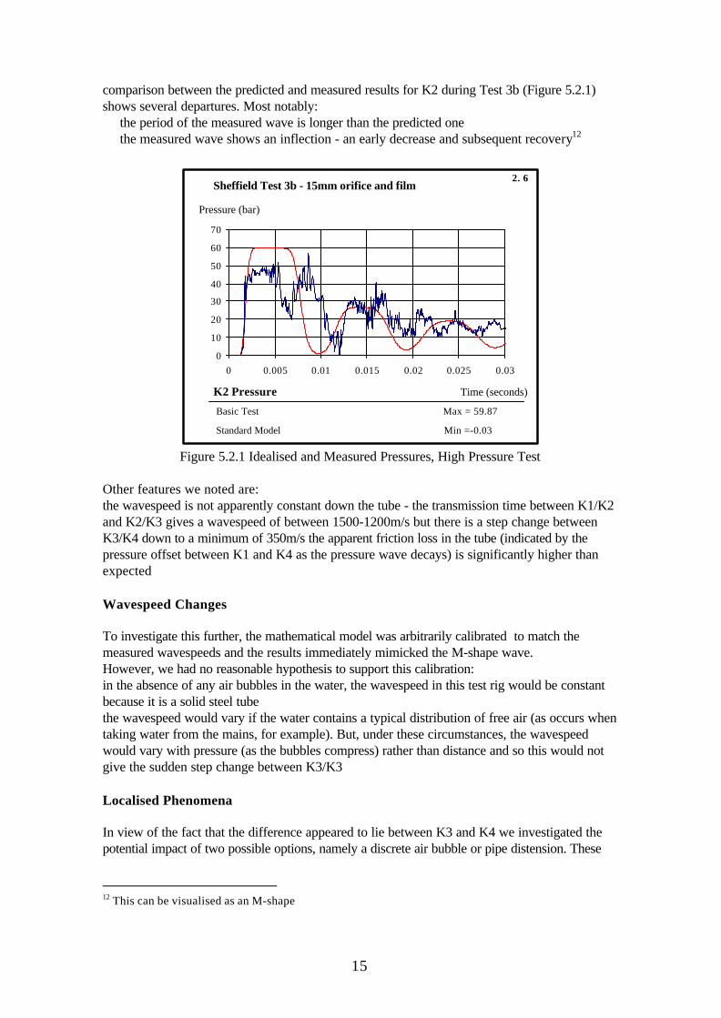
comparison between the predicted and measured results for K2 during Test 3b (Figure 5.2.1)shows several departures. Most notably:
the period of the measured wave is longer than the predicted onethe measured wave shows an inflection - an early decrease and subsequent recovery12
0
10
20
30
40
50
60
70
0 0.005 0.01 0.015 0.02 0.025 0.03
Basic Test
Sheffield Test 3b - 15mm orifice and film
K2 Pressure Time (seconds)
Pressure (bar)
2. 6
Standard Model
Max = 59.87
Min =-0.03
Figure 5.2.1 Idealised and Measured Pressures, High Pressure Test
Other features we noted are:the wavespeed is not apparently constant down the tube - the transmission time between K1/K2and K2/K3 gives a wavespeed of between 1500-1200m/s but there is a step change betweenK3/K4 down to a minimum of 350m/s the apparent friction loss in the tube (indicated by thepressure offset between K1 and K4 as the pressure wave decays) is significantly higher thanexpected
Wavespeed Changes
To investigate this further, the mathematical model was arbitrarily calibrated to match themeasured wavespeeds and the results immediately mimicked the M-shape wave.However, we had no reasonable hypothesis to support this calibration:in the absence of any air bubbles in the water, the wavespeed in this test rig would be constantbecause it is a solid steel tubethe wavespeed would vary if the water contains a typical distribution of free air (as occurs whentaking water from the mains, for example). But, under these circumstances, the wavespeedwould vary with pressure (as the bubbles compress) rather than distance and so this would notgive the sudden step change between K3/K3
Localised Phenomena
In view of the fact that the difference appeared to lie between K3 and K4 we investigated thepotential impact of two possible options, namely a discrete air bubble or pipe distension. These
12 This can be visualised as an M-shape

16
were localised at the site of the orifice/baffle 13 because we were unaware of any other suitablelocation on the tube.The results show that, as with the calibrated wavespeed, the approach of using a short section ofdistensible pipe gives the right trends at K2 but K3/K4 are poor.In contrast, the inclusion of a small air pocket gives fair correlation at all of the transducers,replicating both the initial M-shape and also the amplitude and phasing as the wave decays(Figure 5.2.2).
-10
010
2030
40
5060
7080
90
0 0.01 0.02 0.03 0.04 0.05
Air Bubble Test
Sheffield ST3 with Air at Baffle Site (0.2 litre)
K2 Pressure Time (seconds)
Pressure (bar)
8. 6
Standard Model
Max = 76.35
Min =-.91
Figure 5.2.2 Effect of Air Pocket on High Pressure Test
We did not attempt to optimise the correlation and so, as shown on Figure 5, the prediction over-estimates the second part of the M-wave. But the overall trend is sufficiently close that we feelit clearly illustrates the phenomenon.
Additional Data
We also assessed the additional data (Test 2 and the re-tested results, Test 1b and 3b) andalthough these show some differences, the overall trends are materially unchanged; mostsignificantly, both the M-shape wave and the wavespeed variations still remain.For completeness, the additional data shows:more conformity between tests 1b and 3b, differing as expected only by test-specific factors. Incontrast, the pressures originally recorded at K3 and K4 during Test 1 had been very differentfrom the pressures at the same sites in Tests 2 and 3. But this disparity is eliminated by the re-testing (i.e. Test 1b)some difference between the pressures at K1 in both Test 1b and 3b compared against theoriginal testing. But this is to be expected - this site is the one that is most likely to be affected byblowby from the driver section, one of the reasons for re-testing
Summary
In summary therefore, the results suggest that the new testing procedure has eliminated onesource of unpredictable variation but a further source still remains.
13 We understood that there had been a baffle in the tube for the initial JIP testing

17
We felt that the presence of a small air pocket was the most likely cause of the 'non-standard'behaviour, firstly because of the correlation shown above and secondly because the volume ofair that gives good results differs between the tests. Sheffield University therefore expended agreat deal of time and effort on identifying the 'rogue' phenomenon and eliminating it with revisedtest procedures.
5.3 OPEN TUBE TESTS
Introduction
Our preliminary appraisal of the initial test results suggested that small air pocket(s) were themost likely cause of the 'non-standard' pressure and flow transients. And, as a result, asignificant amount of work was undertaken by Sheffield University to isolate and then eliminatethe air.This section therefore compares the final set of measured results for the Open Tube tests withthe mathematical modelling results.
Test Data
Table 5.3.1Test Summary
Type 4mm Orifice 8mm Orifice 15mm OrificeOpen Tube Test No. 39p - Test No. 37p
Calibration of the Hydraulic Model
The hydraulic model of the shock tube was firstly configured with all the project data (i.e. tubelength, diameter, driver pressure, orifice diameter etc.) to produce an accurate mathematicalrepresentation of the system. However, some parameters, such as the internal hydraulicroughness of the tube and the amount of free air in the test-water are not unique data items andcan vary between systems. The model was therefore calibrated to provide good correlationbetween the measured and predicted results.Using the methodology outlined in the Preliminary Appraisal, the measured data was reviewedfor consistency, smoothed14 and then the wavespeed and friction losses were calibrated.The low pressure test (39p) was then simulated and, using transducer K2 as an example, Figure5.3.1 shows that a reasonable correlation was obtained:
The pressure rises at the same timeThe phasing (periodicity) of the waves is the sameThe peak pressure is similar
14 A limited amount of data smoothing (5 point average) was used to eliminate the most severe of themeasured oscillations

18
0
5
10
15
20
0 0.005 0.01 0.015 0.02
Test 39p - Calibrated
K2 Pressure Time (seconds)
Pressure (bar)
1. 6
Sheffield Model - Calibrated from Test 39p
Max = 18.14
Min = 0
Figure 5.3.1 Preliminary Correlation for Open Tube, Low Pressure Test
Air in the Tube
Although Sheffield University had made significant changes to their test procedures and therebyreduced the amount of air that was trapped within the tube, they noted that some could remainon the downstream side of the filling outlet, on the tube soffit. A small volume was thereforeincluded in the hydraulic model and this immediately introduced the type of pressure inflectionsseen on the measured traces.The volume was therefore calibrated at about 0.025 litres (under initial, atmospheric conditions)and the resulting correlation is given on Figure 5.3.2. For comparison, the high pressure test(37p) was also run on the same model (Figure 5.3.3).
-5
0
5
10
15
20
0 0.005 0.01 0.015 0.02
Test 39p - Calibrated with Air Pocket and Free Air
K3 Pressure Time (seconds)
Pressure (bar)
6. 8
Sheffield Model - Calibrated from Test 39p
Max = 16.90
Min = -0.7
Figure 5.3.2 Correlation for Open Tube, Low Pressure Test

19
0
10
20
30
40
50
60
70
80
0 0.01 0.02 0.03 0.04 0.05
Test 37p - Calibrated from 39p
K3 Pressure Time (seconds)
Pressure (bar)
7. 8
Sheffield Model - Calibrated from Test 39p
Max = 62.47
Min = 0
Figure 5.3.3 Correlation for Open Tube, High Pressure TestCriteria for Acceptance
Our criteria for acceptance of the accuracy of the correlation are based only on the first wave.This generates the pressure conditions that opens the relief device and so the subsequentpressure oscillations are not relevant.Additionally, we have taken position K3 to be the most important for this particular correlation.Although K4 is closer to the end of the shock tube (and therefore closest to the relief device) itprovides very little information in the Open Tube tests because the duration of the pressure waveat this point is too short. K3 is therefore used this correlation.
Review of Results
The hydraulic model used to generate Figure 5.3.2 and Figure 5.3.3 was therefore accepted forthe second phase of the study (i.e. the analysis of the relief device tests) on the basis that:
The initial pressure rises are coincident with the measured testsThe initial rates of pressure rise are the same as the testsThe duration of the pressure waves is the same as the testsThe magnitude of the pressure waves is similar
Summary
Our analysis of the hydraulic modelling and measured results for the Open Tube tests shows thata high level of correlation can be obtained for both of the available tests. Some air remained inthe shock tube under test conditions but the volume was now very small and could be adequatelyaccommodated by calibration.We were therefore confident that the calibrated model could be used for the analysis of the testresults obtained from the relief devices.

20
5.4 GRAPHITE BURST DISC TESTS
Introduction
This section of the report describes the next phase of the modelling study, investigating theresponse times of relief devices; in this case two sets of results from the 4in graphite burst disctests are studied.
Test Data
Table 5.4.1Test Summary
Type 4mm Orifice 8mm Orifice 15mm Orifice4in GraphiteBurst Disc
Test No. 51p - Test No. 49p
The nominal burst pressure for the discs is 15.4 barg.
Test Characteristics
As noted earlier, the tests are completely different in simple terms and this study shows thatthese differences have a significant impact on the action of the relief devices:The 4mm orifice givers a relatively low pressure test. In the Open Tube tests, the peakpressures were only a few bar above the nominal burst pressure of the discs (15.4 barg)The 15mm orifice gives a high pressure test with the disc subjected to a significant, rapidlyapplied pressure which is far higher than the rupture pressure
It is also interesting to note that the university researcher observed a physical manifestation ofthese differences; the graphite discs did not always shatter completely with low pressure tests,occasionally leaving an graphite annulus at the edge of the disc holder.
Mathematical Model of the Burst Discs
Under steady state conditions, the mathematical model used by PSI validates against API RP520 and manufacturers' catalogue data. The aim here was therefore to calibrate the openingtime and thereby confirm the model under dynamic conditions.
Trend Study for High Pressure Test (49p)
The 15mm orifice test was investigated first because this is the 'high' pressure test whichsubjected the disc to a significant pressure wave. This means that the disc ruptured completelywith no likelihood of a residual annulus.Firstly, the hydraulic model of the shock tube was re-configured from the Open Tube tests toinclude a burst disc. Then, a trend study was undertaken to investigate the burst time of the testdisc. In this, all the test parameters remained the same with the exception of one (i.e. the overallburst time of the disc) which was changed systematically.The burst time was taken as the time for the disc to shatter completely. And the results onFigure 5.4.1 and Table 5.4.1 show the effect of parameter on the pressure at K4. The dark line

21
is the measured result and the 3 lighter ones are the simulated result with a disc burst time of 1, 2and 3 msec, respectively.
Table 5.4.1Peak Pressure at K4 from Trend Study
Disc BurstTime (msec)
Peak Pressure (Barg)
1 29.992 41.933 51.60
0
10
20
30
40
50
60
0.004 0.0045 0.005 0.0055 0.006
Test 49p Trend Curve for 1,2, 3 millisec
K4 Pressure Time (seconds)
Pressure (bar)
Sheffield Model - Re-Calibrated after Test 39p
Figure 5.4.1 Trend Study for Graphite Disc, High Pressure Test
Optimising the Burst Time
From these results, the optimum burst time of 1.9 msec was selected and the high pressure test(49p) was re-simulated with this burst time.The results are given for K4 and K2 (Figures 5.4.2 and 5.4.4) and, to demonstrate the high levelof correlation, K4 is also repeated at a very small time scale (Figure 5.4.3). The dark line is thesimulated result.

22
05
1015
2025
3035
4045
0 0.002 0.004 0.006 0.008 0.01 0.012
Test 49p 1.9ms Rupture
K4 Pressure Time (seconds)
Pressure (bar)
1. 10
Sheffield Model - Re-Calibrated after Test 39p
Max = 40.87
Min = 0
Figure 5.4.2 Correlation for Graphite Disc, High Pressure Test
05
1015
2025
3035
4045
0.004 0.0045 0.005 0.0055 0.006
Standard
Test 49p 1.9ms Rupture
K4 Pressure Time (seconds)
Pressure (bar)
1. 10
Sheffield Model - Re-Calibrated after Test 39p
Max = 40.87
Min = 0
Figure 5.4.3 Correlation at K4 over Short Time Scale

23
0
10
20
30
40
50
60
70
80
0 0.002 0.004 0.006 0.008 0.01 0.012
Test 49p 1.9ms Rupture
K2 Pressure Time (seconds)
Pressure (bar)
1. 3
Sheffield Model - Re-Calibrated after Test 39p
Max = 67.30
Min = 0
Figure 5.4.4 Correlation for K2
Discussing the High Pressure Test (49p)
The correlation between the measured and simulated results is exceptionally high for Test 49p,giving a high level of confidence that the mathematical model accurately reflects the action ofthe bursting disc when a 1.9msec burst time is adopted.However, a detailed appraisal of the results shows that, in fact, the duration of the wave at K4 isonly about 0.3 msec from the time when it starts to rise until the time that the pressure peaks.This means that, in this particular test, the results are only sensitive to the disc action for the first15% of the burst time. Thereafter, the disc must have continued to shatter but, with the pressurewave already decaying, this further increase in the relief capacity had no impact.
Low Pressure Test (51p)
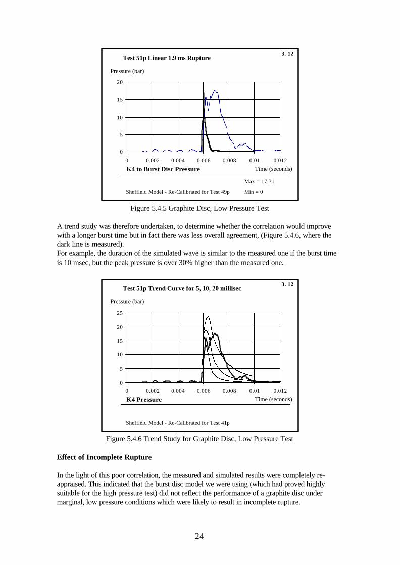
The same burst disc model was adopted for the low pressure test i.e. with a burst time of 1.9msec and the results are given on Figure 5.4.5.Initially, these results show good correlation but the modelled pressure wave then decays almostas soon as the burst disc ruptures whereas the measured wave takes about 2 msec to decay.(The dark line is the simulated result).
24
0
5
10
15
20
0 0.002 0.004 0.006 0.008 0.01 0.012
Test 51p Linear 1.9 ms Rupture
K4 to Burst Disc Pressure Time (seconds)
Pressure (bar)
3. 12
Sheffield Model - Re-Calibrated for Test 49p
Max = 17.31
Min = 0
Figure 5.4.5 Graphite Disc, Low Pressure Test
A trend study was therefore undertaken, to determine whether the correlation would improvewith a longer burst time but in fact there was less overall agreement, (Figure 5.4.6, where thedark line is measured).For example, the duration of the simulated wave is similar to the measured one if the burst timeis 10 msec, but the peak pressure is over 30% higher than the measured one.
0
5
10
15
20
25
0 0.002 0.004 0.006 0.008 0.01 0.012
Test 51p Trend Curve for 5, 10, 20 millisec
K4 Pressure Time (seconds)
Pressure (bar)
3. 12
Sheffield Model - Re-Calibrated for Test 41p
Figure 5.4.6 Trend Study for Graphite Disc, Low Pressure Test
Effect of Incomplete Rupture
In the light of this poor correlation, the measured and simulated results were completely re-appraised. This indicated that the burst disc model we were using (which had proved highlysuitable for the high pressure test) did not reflect the performance of a graphite disc undermarginal, low pressure conditions which were likely to result in incomplete rupture.

25
Obviously, we were not in a position to develop a new model based solely on one set of results;nor do we feel that we would use such a model very often. However, we interrogated themeasured results diagnostically to gain insight into the possible performance of the disc.Firstly, this review showed that the burst disc is able to provide some relief capacity almostinstantly (i.e. within 0.1 msec). This capacity only represents about 2% of the overall capacity(and may therefore be provided by the initial cracks) but, interestingly, this was enough to limitthe pressure rise in this particular low pressure test.Subsequently, for our own interest, we developed a bespoke capacity-model for the low pressuretest, giving the correlation shown on Figure 5.4.7. This was interesting as a correlation exercisebut overall, did not provide any further information about the way in which a graphite discshatters in normal conditions.
0
5
10
15
20
0 0.002 0.004 0.006 0.008 0.01 0.012
Test 51p
K4 Pressure Time (seconds)
Pressure (bar)
3. 12
Sheffield Model - Re-Calibrated for Test 49p
Max = 17.52
Min = 0
Figure 5.4.7 Bespoke Correlation for Graphite Disc, Low Pressure Test
Summary
Our analysis of the hydraulic modelling and measured results for the Graphite Burst Disc testsagain shows that a high level of correlation can be obtained. When the disc was subjected to asignificant, rapidly applied pressure then the (overall) burst time was 1.9 msec. However, resultsare only sensitive to the disc action for the first 15% of the burst time. Thereafter, the disc musthave continued to shatter but, with the pressure wave already decaying, this further increase inthe relief capacity had no impact.In contrast, the findings from the low pressure test were not conclusive. The results suggest thatthe disc provides a small relief capacity almost instantly; although we have no proof, we feel thatthis is possibly in the form of the initial cracks. In turn a small relief flow developed and this wassufficient to reduce the pressures. Thus, for most of the test, the pressure and flow changes inthe shock tube were insensitive to the performance of the burst disc.Overall these results suggests that further work would be beneficial to investigate the 'marginal'conditions, i.e. low pressure cases where the natural system pressures are only slightly higherthan the setting of the relief device. But this is probably low priority when put in context with theaims of the study.This project arose from the investigation into tube rupture within an industrial heat exchangerand, in that context, the rapidly applied high pressure wave is far more important than the
26
marginal, low pressure wave. For such high pressure cases, the results obtained from the highpressure test could be adopted, within an overall burst time of 1.9 msec.
5.5 STAINLESS STEEL BURST DISC TESTS
Introduction
This section continues the examination of the burst discs, this time looking at the stainless steeldiscs.
Test Data
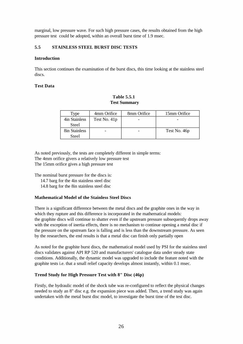
Table 5.5.1Test Summary
Type 4mm Orifice 8mm Orifice 15mm Orifice4in Stainless
SteelTest No. 41p - -
8in StainlessSteel
- - Test No. 46p
As noted previously, the tests are completely different in simple terms:The 4mm orifice givers a relatively low pressure testThe 15mm orifice gives a high pressure test
The nominal burst pressure for the discs is:14.7 barg for the 4in stainless steel disc14.8 barg for the 8in stainless steel disc
Mathematical Model of the Stainless Steel Discs
There is a significant difference between the metal discs and the graphite ones in the way inwhich they rupture and this difference is incorporated in the mathematical models:the graphite discs will continue to shatter even if the upstream pressure subsequently drops awaywith the exception of inertia effects, there is no mechanism to continue opening a metal disc ifthe pressure on the upstream face is falling and is less than the downstream pressure. As seenby the researchers, the end results is that a metal disc can finish only partially open
As noted for the graphite burst discs, the mathematical model used by PSI for the stainless steeldiscs validates against API RP 520 and manufacturers' catalogue data under steady stateconditions. Additionally, the dynamic model was upgraded to include the feature noted with thegraphite tests i.e. that a small relief capacity develops almost instantly, within 0.1 msec.
Trend Study for High Pressure Test with 8" Disc (46p)
Firstly, the hydraulic model of the shock tube was re-configured to reflect the physical changesneeded to study an 8" disc e.g. the expansion piece was added. Then, a trend study was againundertaken with the metal burst disc model, to investigate the burst time of the test disc.

27
The results on Figure 5.5.1 and Table 5.5.2 show the effect of the burst time on the pressure atK4. The dark line is the measured result and the 3 lighter ones are the simulated result with adisc burst time of 5, 10 and 15 msec, respectively.
Table 5.5.2Peak Pressure at K4 from Trend Study
Disc BurstTime (msec)
Peak Pressure(Barg)
5 18.9510 19.4415 21.50
0
5
10
15
20
25
0 0.002 0.004 0.006 0.008 0.01 0.012
Test 46p Trend Curve for 5, 10 and 12 millisec
K4 Pressure Time (seconds)
Pressure (bar)
Sheffield Model - Taken from Test 51p
Figure 5.5.1 Trend Curve for 8" Metal Disc, High Pressure Test
Optimising the Burst Time
From these results, the optimum burst time of 10 msec was selected and the results are given forK4 (Figure 5.5.2). The dark line is the simulated result.

28
0
5
10
15
20
25
0 0.002 0.004 0.006 0.008 0.01 0.012
Test 46p 10ms Rupture
K4 Pressure Time (seconds)
Pressure (bar)
5. 10
Sheffield Model - Taken from Test 51p
Max = 19.44
Min = 0
Figure 5.5.2 Correlation for 8" Metal Disc, High Pressure Test

29
Discussing the High Pressure Test (46p)
The test rig had been re-configured for this test to include a 4in-8in expansion and this, in itself,introduced additional pressure changes in the shock tube. But despite this, we show goodcorrelation for a metal disc by incorporating the features shown with the graphite disc (i.e. of aninitial, immediate opening of a few percent) and an effective time of 10 msec.
Low Pressure Test with 4in Disc (41p)
The final correlation for the burst discs was Test 41p which studies a 4in metal disc. The modelused in the previous cases was therefore simulated and the results are shown on Figure 5.5.3.This again shows reasonable correlation based on an initial immediate opening of a few percentfollowed by an effective opening time of 10 msec. But as seen with the previous test, relief ofthe pressure wave is achieved with less than 10 percent of the total disc capacity and so anaccurate estimation of the overall opening time is difficult.
0
5
10
15
20
25
0 0.002 0.004 0.006 0.008 0.01 0.012
Test 41p 10ms Rupture
K4 Pressure Time (seconds)
Pressure (bar)
4. 8
Sheffield Model - Taken from Test 51p
Max = 19.96
Min = 0
Figure 5.5.3 Correlation for 4in Metal Disc, Low Pressure Test
Disc Performance: Graphite versus Metal
In addition to investigating the opening times for the different devices we undertook acomprehensive appraisal of each set of results, with comparison against the original open tubetests and also comparing different relief devices (see Appendix B). And this was particularlyinteresting when examining the burst disc results.For example, we earlier outlined the need for two different disc models, one for graphite and onefor metal discs and this difference is apparent when examining the test results for the K4transducer (Figure 5.5.4).

30
Position K4 for 4in Graphite and SS Discs
-5
0
5
10
15
20
0 0.002 0.004 0.006 0.008 0.01 0.012
Time (s)
Pre
ss
ure
(b
ar)
K4, 51p, 4inGraphite
K4 41p, 4in SS
Figure 5.5.4 Measured Test at K4 - Graphite and Metal Discs
Figure 5.5.4 shows the low pressure tests for both 4" discs and hence are directly comparablebut their performance is different:The capacity15 of the graphite disc is high enough that the device offered no restriction to theflow in the shock tube after it had ruptured. This means that the pressure at K4 dropped toatmospheric pressure by about 8 msecThe metal disc only opened partially and offered significant restriction to the flow in the shocktube. This means that the pressure at K4 remained at almost 10 bar. Subsequently, the pressurethroughout the shock tube dropped, as discussed in Appendix A
Summary
We have two different models for burst discs, one for graphite discs (in which the relief capacitycontinues to increase to the maximum once it starts to rupture) and one for metal discs (whichonly opens when there is a positive driving force). And the this study has confirmed the need fortwo different models.The results also show that the metal discs opened more slowly than the graphite discs (nominallyin 10 msec compared with only 1.9 msec for the graphite discs). And, subjectively a slower timeis expected because of the difference in the disc material and the manner in which theyopen/shatter. However, the discs studied in the high pressure tests16 are also different sizes (theslower disc is also the larger) and so it is not possible to state whether the difference in openingtime is only attributable to the material or whether it is also a function of size.Additionally, we have some reservations about the accuracy of the burst time for the metal disc(10 msec). As seen with the graphite disc, the pressure wave was relieved within about 10% ofthe opening time and this means, subsequently, the test became insensitive to the disc capacity.
15 Although it is impossible to say whether the graphite disc shattered completely (or whether a smallannulus remained), either way, it gave materially the full capacity16 The high pressure tests give a more reliable burst time

31
In practice therefore the overall burst time represents an effective rupture period of about 1msec, extrapolated to give an overall estimate of 10 msec.Overall, the study again shows good correlation between the measured and simulated results andwe have a high level of confidence in the model. But we suggest that further work is undertakento examine this in more detail:
with a wider range of tests that are directly comparable,under tests conditions that sensitive to the disc capacity and hence give a more accurate estimation of the overall opening time
5.6 SPRING LOADED RV, HIGH PRESSURE TEST
Introduction
This section continues the examination of the relief devices, starting to look at the spring loadedrelief valves (RVs).17
Test Data
As noted previously, the 15mm orifice gives a high pressure test. The equivalent low pressuretest is discussed later in the section.
Table 5.6.1Test Summary
Type 4mm Orifice 8mm Orifice 15mm Orifice2in SpringLoaded
See Section5.7
- Test 57p
The set pressure for the RV is 15 barg.
Mathematical Model of the Spring Loaded RVs
As noted for the burst discs, the mathematical model used by PSI for the spring loaded reliefvalve validates against API RP 520 and manufacturers' catalogue data under steady stateconditions. However, the dynamic model also incorporates the unique characteristics of the valveaction, described in the manufacturers' catalogues with the specific terms 'pop open' and'blowdown'.In brief the cycle of an RV is:ClosedValve starts to 'simmer' when local pressure exceeds set pressureValve pops open at popping point (i.e. a pressure slightly above the set pressure). When thevalve has popped open, the rated capacity is in accordance with the international codes i.e. at110% of set pressureFurther lift is proportional to pressure to give slightly more capacityIn the initial closing phase, lift is proportional to pressure
17 The simple difference between a burst disc and a relief valve (as defined in API RP 520) is the fact thatthe burst disc is a non-closing device whilst an RV is designed to automatically re-close and prevent thefurther flow of fluid.

32
Then the valve blows down, with a smaller pop action, down to closure at a lower (blowdown)pressure. The cycle is now complete with the valve re-closed.

33
Opening Time for RVs
As noted above, the 'rated' capacity18 of an RV is reached when it pops open and this is themost important feature of the valves. We have therefore defined the opening time for RVs asthe time taken to reach the rated capacity i.e. the capacity for 110% of the set pressure, or 10%over-pressure (10% OP).
Trend Study for High Pressure Test (57p)
Firstly, the hydraulic model of the shock tube was re-configured to incorporate the RV and then,a trend study was again undertaken to investigate the opening time.The results are given on Table 5.6.2 and Figure 5.6.1, the dark line is measured.
Table 5.6.2 Peak Pressure at K4 from Trend Study
RV 10% OPTime (msec)
Peak Pressure(Barg)
1.5 87.03.0 97.24.5 102.16.0 104.9
0
20
40
60
80
100
120
0 0.002 0.004 0.006 0.008 0.01 0.012
Test 57p Trend Curve for 1.5, 3 4.5 & 6millisec
K4 Pressure Time (seconds)
Pressure (bar)
Sheffield Model - Taken from Test 51p
Figure 5.6.1 Trend Curve for Spring RV, High Pressure Test
Optimising Opening Time
18 The 'rated' capacity is in accordance with international codes

34
From these results, the optimum opening time of 4 msec was selected and the high pressure testwas re-simulated with this time.The results are given for K4 and K3 (Figures 5.6.2 and 5.6.3, the dark lines are the simulatedresult) and these again show very good correlation.
-20
0
20
40
60
80
100
120
0 0.002 0.004 0.006 0.008 0.01 0.012
Test 57p 10% Capacity in 4ms
K4 Pressure Time (seconds)
Pressure (bar)
5. 8
Sheffield Model - Taken from Test 51p
Max = 100.75
Min = 0
Figure 5.6.2 Correlation for Spring RV, High Pressure Test
-20
0
20
40
60
80
100
120
0 0.002 0.004 0.006 0.008 0.01 0.012
Test 57p 10% Capacity in 4ms
K3 Pressure Time (seconds)
Pressure (bar)
5. 12
Sheffield Model - Taken from Test 51p
Max = 101.28
Min = 0
Figure 5.6.3 Correlation for K2
Evaluation of the Results
Our evaluation of the tests results also highlighted two other features:RV remains fully opening for the test period. As shown on Figure 5.6.4, the pressure in theshock tube remains well above the set pressure of the RV (15 barg)As might be expected, the capacity of the 2in RV is far lower than the capacity of the 4in burstdisc. Additionally, the burst disc reacts more quickly. For example, in comparable tests, the

35
graphite burst disc limited the peak pressure to about 41 barg and reduced the pressure at K4towards atmospheric pressure. In contrast the peak pressure is over 100 barg with the 2in RVand the pressure at K4 remains above 60 barg for the remainder of the test.
2in Spring Relief - 15mm
0
20
40
60
80
100
120
0 0.05 0.1 0.15
Time (s)
Pre
ss
ure
(b
arg
) K4
Figure 5.6.4 Measured Test at K4 - Spring Loaded RV
Summary
The mathematical model for the RV is far more complex than the burst disc model as it needs toreflect the complete performance cycle of pop open and then blowdown. But despite this we areagain able to show good correlation when with an opening time of 4 msec. However, it must beremembered that this opening time is defined very specifically for RVs as the time taken toreach the rated capacity i.e. the capacity for 110% of the set pressure, or 10% over-pressure(10% OP).
5.7 SPRING LOADED RV, LOW PRESSURE TEST
Introduction
This section discusses the findings of the low pressure test on the spring loaded RV.
Test Data
The test and number is that used by Sheffield University. As noted previously, the 4mm orificegives a low pressure test.
Table 5.7.1Test Summary
Type 4mm Orifice 8mm Orifice 15mm Orifice2in SpringLoaded
Test 59p - Section 5.6

36
The set pressure for the RV is 15 barg.
37
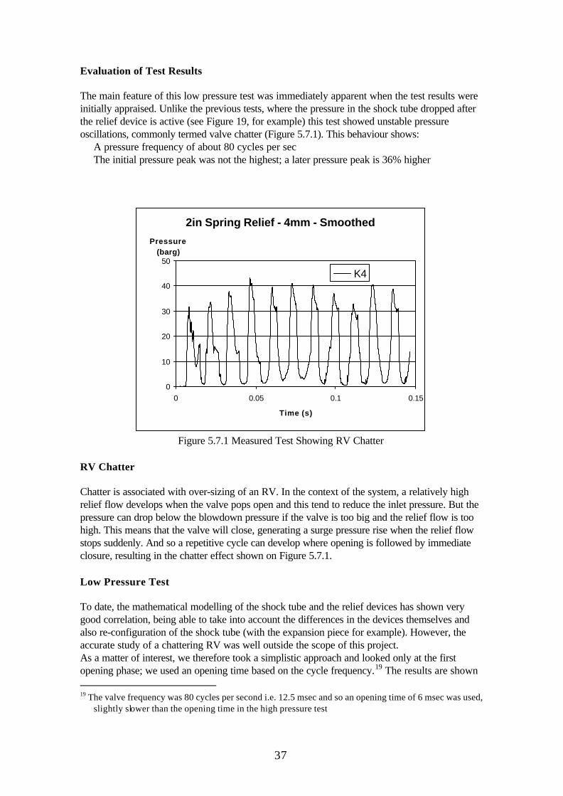
Evaluation of Test Results
The main feature of this low pressure test was immediately apparent when the test results wereinitially appraised. Unlike the previous tests, where the pressure in the shock tube dropped afterthe relief device is active (see Figure 19, for example) this test showed unstable pressureoscillations, commonly termed valve chatter (Figure 5.7.1). This behaviour shows:
A pressure frequency of about 80 cycles per secThe initial pressure peak was not the highest; a later pressure peak is 36% higher
2in Spring Relief - 4mm - Smoothed
0
10
20
30
40
50
0 0.05 0.1 0.15
Time (s)
Pressure (barg)
K4
Figure 5.7.1 Measured Test Showing RV Chatter
RV Chatter
Chatter is associated with over-sizing of an RV. In the context of the system, a relatively highrelief flow develops when the valve pops open and this tend to reduce the inlet pressure. But thepressure can drop below the blowdown pressure if the valve is too big and the relief flow is toohigh. This means that the valve will close, generating a surge pressure rise when the relief flowstops suddenly. And so a repetitive cycle can develop where opening is followed by immediateclosure, resulting in the chatter effect shown on Figure 5.7.1.
Low Pressure Test
To date, the mathematical modelling of the shock tube and the relief devices has shown verygood correlation, being able to take into account the differences in the devices themselves andalso re-configuration of the shock tube (with the expansion piece for example). However, theaccurate study of a chattering RV was well outside the scope of this project.As a matter of interest, we therefore took a simplistic approach and looked only at the firstopening phase; we used an opening time based on the cycle frequency.19 The results are shown 19 The valve frequency was 80 cycles per second i.e. 12.5 msec and so an opening time of 6 msec was used,
slightly slower than the opening time in the high pressure test

38
on Figure 5.7.2 and Figure 5.7.3 and the overall correlation is good. But it already under-estimates the oscillation seen at K4, i.e. near the RV.
Summary
The low pressure test on the spring loaded relief valve showed all the characteristics of valvechatter, consistent with the performance of an over-sized valve. The detailed study of thisphenomenon was well outside the scope of this study and so only the initial pop-open phase wasstudied. And this suggested that the RV opened slightly slower in this test than in the highpressure test (6 msec compared with 4 msec). However, some pressure oscillation is stillapparent, even within this opening stage.
-10
0
10
20
30
40
50
0 0.002 0.004 0.006 0.008 0.01 0.012
Test 59p 10% Capacity in 6ms
K4 Pressure Time (seconds)
Pressure (bar)
6. 8
Sheffield Model - Taken from Test 51p
Max = 27.38
Min = 0
Figure 5.7.2 Preliminary Correlation for RV, Low Pressure Test
-10
0
10
20
30
40
50
0 0.002 0.004 0.006 0.008 0.01 0.012
Test 59p 10% Capacity in 6ms
K3 Pressure Time (seconds)
Pressure (bar)
6. 12
Sheffield Model - Taken from Test 51p
Max = 27.39
Min = 0
Figure 5.7.3 Correlation for K3

39
5.8 PILOT OPERATED RELIEF VALVE TEST
Introduction
This section discusses the final set of results, namely for the pilot operated relief valve.
Test Data
As noted previously, the 4mm orifice gives a low pressure test and the 15mm is a high pressuretest.
Table 5.8.1Test Summary
Type 4mm Orifice 8mm Orifice 15mm Orifice2in Pilot RV Test 66p - Test 64p
The set pressure for the RV is 15 barg.
Valve Characteristics
Although the pilot operated RV is nominally the same size as the spring loaded RV discussed inthe preceding section, the capacity of a pilot operated valve is slightly greater. It is also worthnoting that, physically, this pilot valve is more compact and most importantly the moving parts ofthe valve are smaller than the spring loaded RV. And, overall, these factors mean that weexpected the pilot operated valve to react slightly more quickly than the spring loaded valve.Additionally, the pilot configuration offers either pop-action or modulating-action; there is also acombined option of pop-open and modulate-closed which was the configuration studied in thesetests. And again, this means that the test valves were the fastest available.Opening Time for RVsAs noted earlier, the 'rated' capacity20 of an RV is reached when it pops open and this is themost important feature of the valves. We have therefore defined the opening time for RVs asthe time taken to reach the rated capacity i.e. the capacity for 110% of the set pressure, or 10%over-pressure (10% OP).
Trend Study for High Pressure Test (64p)
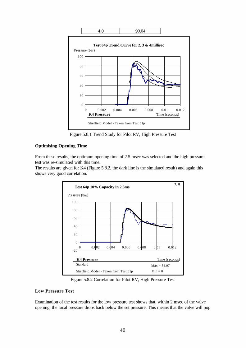
As before, the hydraulic model of the shock tube was re-configured to incorporate the pilotoperated RV and a trend study was again undertaken to investigate the opening time.The results are given on Table 5.8.2 and Figure 5.8.1, where the dark line is measured.
Table 5.8.2Peak Pressure at K4 from Trend Study
RV 10% OPTime (msec)
Peak Pressure(Barg)
2.0 81.043.0 86.66
20 The 'rated' capacity is in accordance with international codes
40
4.0 90.04
0
20
40
60
80
100
0 0.002 0.004 0.006 0.008 0.01 0.012
Test 64p Trend Curve for 2, 3 & 4millisec
K4 Pressure Time (seconds)
Pressure (bar)
Sheffield Model - Taken from Test 51p
Figure 5.8.1 Trend Study for Pilot RV, High Pressure Test
Optimising Opening Time
From these results, the optimum opening time of 2.5 msec was selected and the high pressuretest was re-simulated with this time.The results are given for K4 (Figure 5.8.2, the dark line is the simulated result) and again thisshows very good correlation.
-20
0
20
40
60
80
100
0 0.002 0.004 0.006 0.008 0.01 0.012
Standard
Test 64p 10% Capacity in 2.5ms
K4 Pressure Time (seconds)
Pressure (bar)
7. 8
Sheffield Model - Taken from Test 51p
Max = 84.07
Min = 0
Figure 5.8.2 Correlation for Pilot RV, High Pressure Test
Low Pressure Test
Examination of the test results for the low pressure test shows that, within 2 msec of the valveopening, the local pressure drops back below the set pressure. This means that the valve will pop

41
open and then immediately start to modulate closed. However, this is a function of the type andconfiguration of the pilot system and the accurate study of its performance was well outside thescope of this project.Again, as a matter of interest, we therefore took a simplistic approach and looked only at thefirst opening phase; the opening time was taken as 4 msec, based on earlier findings of this studythat the devices tend to act more slowly in the marginal, low pressure tests, compared with thehigh pressure ones. The results are shown on Figure 5.8.3, where the dark line is simulated.
-5
0
5
10
15
20
25
30
0 0.002 0.004 0.006 0.008 0.01 0.012
Test 66p 10% Capacity in 4ms
K4 Pressure Time (seconds)
Pressure (bar)
8. 8
Sheffield Model - Taken from Test 51p
Max = 22.11
Min = 0
Figure 5.8.3 Correlation for Pilot RV, Low Pressure Test
RV Performance: Spring Loaded versus Pilot
Pilot operated RVs are not widely used in industry. As stated in API RP 520, "since the mainvalve and pilot contain non metallic components, process temperature and fluid compatibility limittheir use. In addition, fluid characteristics such as a susceptibility to polymerisation, fouling,viscosity, the presence of solids and corrosiveness may affect pilot reliability".Despite this, as shown on Figure 5.8.4, their modulating action may by beneficial. The severechatter exhibited by the spring loaded RV is completely eliminated from the low pressure testand replaced by stable performance.

42
Position K4 Relief Valve
-5
0
5
10
15
20
25
30
35
40
45
50
0 0.05 0.1
Time (s)
Pre
ss
ure
(b
ar)
K4, 66p, Pilot
K4 59p, Spring
Figure 5.8.4 Measured Test at K4 - Spring Loaded and Pilot RV
Summary
The study shows that the 2in spring loaded RV popped open in 4 msec compared with 2.5 msecfor the pilot operated valve. And this finding, was unexpected. Subjectively, a slower responsewas expected. However, we note that:The pilot operated RV and the spring loaded RV are not directly similar valves. The physicalmass of the moving parts is smaller for the pilot operated valve and so the inertia effects wouldbe lowerWe do not have details of the pilot system for the valve but the findings of the study suggest thatit is the type that is characterised by pop action, followed by a modulating action.21 This meansthat the opening performance will not be adversely affected by the pilot
The study also shows that the modulating action is particularly beneficial in eliminating the severevalve chatter seen previously with the spring loaded RV. However, this is not the only way ofeliminating chatter. It can also be avoided by other means, for example, by using dynamicsimulation methods to ensure that the spring loaded RV is correctly sized in the design stage.
21 This is supported by the valve performance in the low pressure test
43
6. CONCLUSIONS AND RECOMMENDATIONS FOR FURTHER WORK
The study was initiated as a result of concerns over the failure of pressure vessels holding liquidswhen subjected to internal pressure pulses whose amplitudes and durations were above certainlimiting values. Whilst pressures higher than yield pressure may be tolerated for durations whichare short compared to some characteristic time of the structure, the effect of delayed pressurerelief is expected to extend the period of higher pressure exposure and hence may move thetransient into a hazard range.
The study emphasises a few key features associated with the pressurising source andsubsequent wave propagation, and these can be summarised as follows :
1. following gas release there is a constant pressure which develops at the liquid/gas interface and this pressure propagates at sound speed in the liquid, being experienced by the structure following its passage. The constant pressure will depend on the rate of flow of gas into the interface region and the compressibility of the downstream liquid. This is characterised by a plateau region on the upstream transducers (K2, K3) in the study.
2. On arrival at the relief device, the pressure wave opens the device after a certain time and this then propagates an expansion wave upstream which cancels the high pressure. For
instantaneous opening, the duration of the high pressure exposure upstream is solelydependent on the distances involved and the sound speed in the liquid. For water filled vesselsthis corresponds approximately to 0.7msec/meter pathlength, where the pathlength is theround-trip distance from any point to the relief device.
3. Any delay in the opening of the device will result in the reflection of a pressure wave of twice the amplitude upstream and therefore the exposures which should be of concern are the initial plateau pressure, the reflected wave pressure and the duration associated with each. The
plateau duration has been referred to above. The reflected wave duration will depend on theopening time of the device, and a number of data traces show this effect.
4. The analysis has indicated that for the devices tested, times to full opening are 1.9 - 10 msecfor the bursting discs and 2.5 - 4 msec for the RVs. The differences in the relative scale ofthese two families of devices has already been emphasised and is reiterated here.
5. Whilst the study used oversized discs and undersized RVs, the quoted times should strictly beapplied to pressurising systems for which the devices would represent the correct sizes.
6. It is considered that the timescales for opening are significant and are comparable with theresponse times for structures as they move toward yield when exposed to a step pressure
rise. A transient analysis is therefore considered a worthwhile exercise during the design of low pressure vessels which may be exposed to high pressure transients, whose relief is

44
governed by RV or bursting disc behaviour. In summary, the opening times to full relief capacityfor a number of the devices tested are collected together in Table 6.1.
Table 6.1Measured relief times for selected relief devices
Relief device Conditions Relief time - msecGraphite 4" high pressure 1.9
Stainless steel 8" high pressure 10Stainless steel 4" low pressure 10
Relief valve high pressure 4Relief valve low pressure 6
Pilot operated relief valve high pressure 2.5Pilot operated relief valve low pressure 4
We recommend that further work is undertaken to determine the dependency of these findingson pressure conditions. Although we have nominally undertaken a detailed analysis of two setsof results (high and low pressure), only the high pressure tests were effective in terms of the fullopening of the devices. We therefore suggest that we take advantage of the fact that SheffieldUniversity already have another set of measured data available (8mm tests) and repeat thedetailed analysis on this information.To determine whether the apparently slow opening of the metal disc is due predominantly to itssize we also suggest that we analyse the existing test data for the 4" metal disc.Turning to the RVs, we feel that there are two areas of investigation available. The first, andpotentially the most conclusive, would be to undergo further physical testing on different valvesizes and types. The second would combine the skills of detailed analysis and literature review toexplore the basis for the longer opening times for the RVs that were given in the IP guidelinesand in other research papers. The work should focus on points of comparison e.g. establishingwhether the valves were the same type (pop action) and size.

45
7. APPENDIX
7.1 PHOTOGRAPHS
A number of photographs illustrate the key components used in carrying out the experimental
study.

46
Plate 1. Working area for shock tube control and data collection

47
Plate 2 Aluminium driver diaphragm controlling driver operating pressure - before and after rupture
Plate 3. Driver diaphragm in place after firing - driver section on the right.

48
Plate 4. The three discharge orifices used in the tests
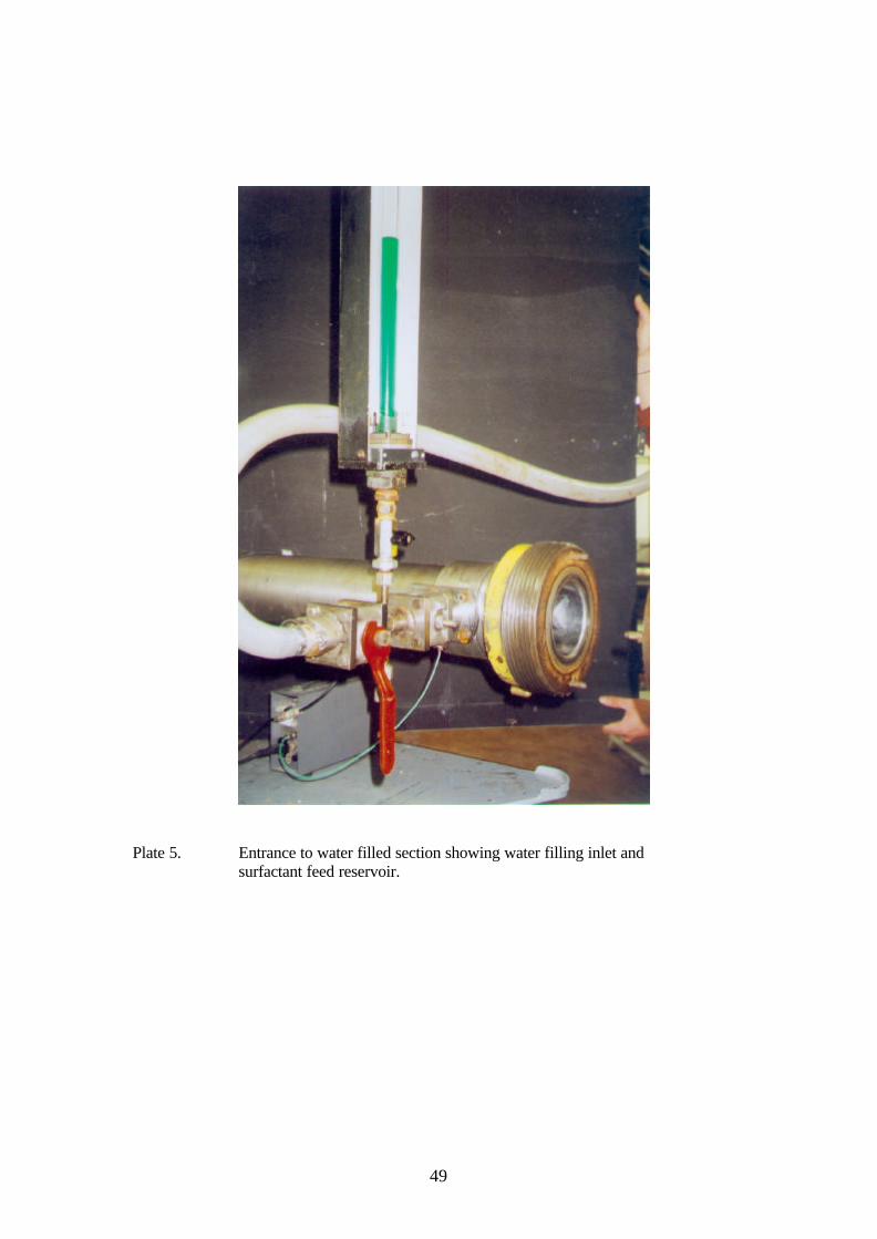
49
Plate 5. Entrance to water filled section showing water filling inlet andsurfactant feed reservoir.

50
Plate 6. Samples of 4" and 8" stainless steel bursting discs before firing
Plate 7. 8" disc and holder

51
Plate 8. Expansion section for 8" stainless bursting disc.

52
Plate 9. Graphite disc holder in place at outlet end of shock tube.
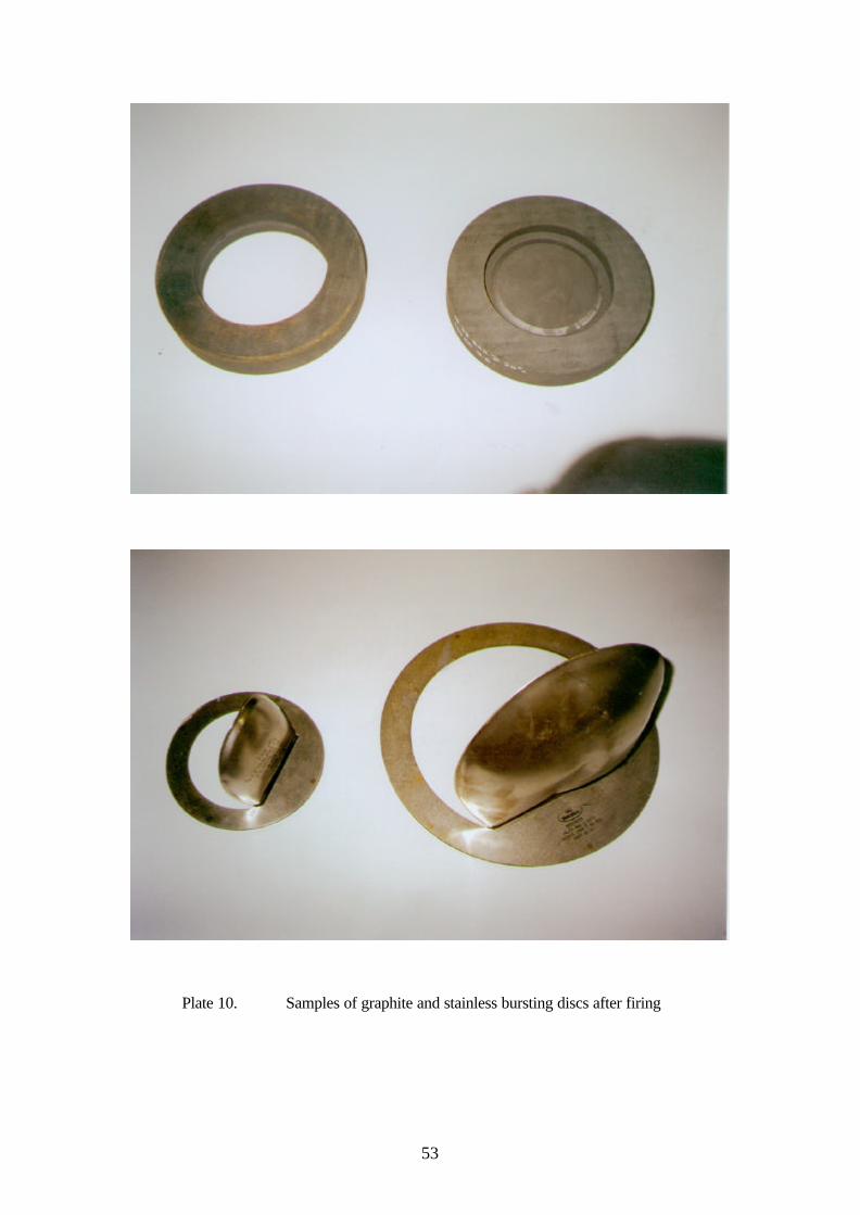
53
Plate 10. Samples of graphite and stainless bursting discs after firing

54
Plate 11. 2" relief valve body used in valve tests.

55
7.2 DATA CHARTS
The data charts represent up to 50 msec of pressure data following driver disc rupture.
Full records are actually 250msec in duration.

56
-2 -1 0 1 2 3 4 5 6 7 8 9 10-5
0
5
10
15
20
25Test 39 4mm orifice, plastic
film at outlet
Pre
ssu
re -
bar
msec
K1 K2 K3 K4
CHART A.1
-2 -1 0 1 2 3 4 5 6 7 8 9 10-10
0
10
20
30
40
50
608mm orifice, plastic film at outlet
Pre
ssu
re -
bar
msec
Test 38
K1 K2 K3 K4
CHART A.2

57
-2 -1 0 1 2 3 4 5 6 7 8 9 10-20
0
20
40
60
80
100
12015mm orifice, plastic film at outlet
Pre
ssu
re -
bar
msec
Test 37
K1 K2 K3 K4
CHART A.3
-2 -1 0 1 2 3 4 5 6 7 8 9 10-5
0
5
10
15
20
25
30 4mm orifice, 4" graphite disc
Pre
ssu
re -
bar
msec
Test 51
K1 K2 K3K4
CHART A.4

58
-2 -1 0 1 2 3 4 5 6 7 8 9 10-10
0
10
20
30
40
50
60
70 8mm orifice, 4" graphite disc
Pre
ssu
re -
bar
msec
Test 50
K1 K2K3
K4
CHART A.5
-2 -1 0 1 2 3 4 5 6 7 8 9 10-20
0
20
40
60
80
100
120 15mm orifice, 4" graphite disc
Pre
ssu
re -
bar
msec
Test 49
K1 K2
K3
K4
CHART A.6

59
-2 -1 0 1 2 3 4 5 6 7 8 9 10-5
0
5
10
15
20
25
30 4mm orifice, 6" graphite disc
Pre
ssu
re -
bar
msec
Test 55
K1
K2
K3K4
CHART A.7
-2 -1 0 1 2 3 4 5 6 7 8 9 10-40
-20
0
20
40
60
808mm orifice, 6" graphite disc
Pre
ssu
re -
bar
msec
Test 54
CHART A.8

60
-2 -1 0 1 2 3 4 5 6 7 8 9 10
0
20
40
60
80
100
120 15mm orifice, 6" graphite disc
Pre
ssu
re -
bar
msec
Test 53
K1 K2K3 K4
CHART A.9
-2 -1 0 1 2 3 4 5 6 7 8 9 10 11 12-5
0
5
10
15
20
25
304mm orifice, 4" stainless steel disc
Pre
ssu
re -
bar
msec
Test 41
K1 K2 K3 K4
CHART A.10

61
-2 -1 0 1 2 3 4 5 6 7 8 9 10-10
0
10
20
30
40
50
60
70
80P
ress
ure
- b
ar
msec
Test 42 8mm orifice, 4" stainless steel disc
K1K2 K3 K4
CHART A.11
-2 -1 0 1 2 3 4 5 6 7 8 9 10-20
0
20
40
60
80
100
120
Pre
ssu
re -
bar
msec
Test 40 15mm orifice, 4" stainless steel disc
K1 K2 K3 K4
CHART A.12

62
-2 -1 0 1 2 3 4 5 6 7 8 9 10-10
0
10
20
30
40
50
Pre
ssu
re -
bar
msec
Test 47 8mm orifice, 8" stainless steel disc
K1 K2K3 K4
CHART A.14
-2 -1 0 1 2 3 4 5 6 7 8 9 10-10
0
10
20
30
40P
ress
ure
- b
ar
msec
Test 48 4mm orifice, 8" stainless steel disc
K1 K2 K3 K4
CHART A.13

63
-2 -1 0 1 2 3 4 5 6 7 8 9 10-20
0
20
40
60
80
100
120P
ress
ure
- b
ar
msec
Test 46 15mm orifice, 8" stainless steel disc
K1 K2 K3K4
CHART A.15
-10
12
34
56
78
910
1112
1314
15-20
-10
0
10
20
30
40
50 4mm orifice, 2" relief valve
Pre
ssu
re -
bar
msec
Test 59
K1K2 K3 K4
CHART A.16

64
0 5 10 15 20 25 30 35 40 45 50-20
-10
0
10
20
30
40
50 4mm orifice, 2" relief valve
Pre
ssu
re -
bar
msec
Test 59
CHART A.17
-10
12
34
56
78
910
1112
1314
15-10
0
10
20
30
40
50
60
70 8mm orifice, 2" relief valve
Pre
ssu
re -
bar
msec
Test 58
K1 K2 K3 K4
CHART A.18

65
0 5 10 15 20 25 30 35 40 45 50-10
0
10
20
30
40
50
60
70 8mm orifice, 2" relief valve
Pre
ssu
re -
bar
msec
Test 58
CHART A.19
-10
12
34
56
78
910
1112
1314
15-20
0
20
40
60
80
100
120
Pre
ssu
re -
bar
msec
Test 57 15mm orifice, 2" relief valve
K1 K2 K3 K4
CHART A.20

66
0 5 10 15 20 25 30 35 40 45 50-20
0
20
40
60
80
100
120P
ress
ure
- b
ar
msec
Test 57 15mm orifice, 2" relief valve
CHART A.21
-10
12
34
56
78
910
1112
1314
15-10
0
10
20
30
40Test 62 4mm orifice, 2"
bellows relief valve
Pre
ssu
re -
bar
msec
K1K2 K3
K4
CHART A.22

67
0 5 10 15 20 25 30 35 40 45 50-10
0
10
20
30
40Test 62 4mm orifice, 2"
bellows relief valve
Pre
ssu
re -
bar
msecCHART A.23
-10
12
34
56
78
910
1112
1314
15-20
-10
0
10
20
30
40
50
60
70
Pre
ssu
re -
bar
msec
Test 61 8mm orifice, 2" bellows relief valve
K1 K2 K3 K4
CHART A.24

68
0 5 10 15 20 25 30 35 40 45 50-20
-10
0
10
20
30
40
50
60
70P
ress
ure
- b
ar
msec
Test 61 8mm orifice, 2" bellows relief valve
CHART A.25
-10
12
34
56
78
910
1112
1314
15-20
0
20
40
60
80
100
12015mm orifice, 2" bellows relief valve
Pre
ssu
re -
bar
msec
Test 60
K1
K2 K3 K4
CHART A.26

69
0 5 10 15 20 25 30 35 40 45 50-20
0
20
40
60
80
100
120Test 60
15mm orifice, 2" bellows relief valve
Pre
ssu
re -
bar
msecCHART A.27
-10
12
34
56
78
910
1112
1314
15-10
0
10
20
30Test 66 4mm orifice, 2"
pilot assistedrelief valve
Pre
ssu
re -
bar
msec
K2 K3K4
K1
CHART A.28

70
0 5 10 15 20 25 30 35 40 45 50-10
0
10
20
304mm orifice, 2" pilot assistedrelief valve
Pre
ssu
re -
bar
msec
Test 66
CHART A.29
-10
12
34
56
78
910
1112
1314
15-10
0
10
20
30
40
50
60
Pre
ssu
re -
bar
msec
8mm orifice, 2" pilot assisted relief valve
Test 65
K1 K2 K3
K4
CHART A.30

71
0 5 10 15 20 25 30 35 40 45 50-10
0
10
20
30
40
50
60P
ress
ure
- b
ar
msec
8mm orifice, 2" pilot assisted relief valve
Test 65
CHART A.31
-10
12
34
56
78
910
1112
1314
15-20
0
20
40
60
80
100
Pre
ssu
re -
bar
msec
15mm orifice, 2" pilot assisted relief valve
Test 64
K1K2 K3 K4
CHART A.32

72
0 5 10 15 20 25 30 35 40 45 50-20
0
20
40
60
80
100P
ress
ure
- b
ar
msec
15mm orifice, 2" pilot assisted relief valve
Test 64
CHART A.33

73
7.3 VIDEO TAPE RECORD
The following is a brief review in sequence of the content of the 13 minute video tapeaccompanying the report.
1. Panning view of shock tube with driver section to the left and water filled section at the right. At the right hand end can be seen the conical expansion and holder for the 200 mm stainless steel bursting disc.
2. Close-up of the driver aluminium diaphragm after firing followed by one of the Kistler transducer amplifier boxes.
3. Close-up of 200 mm expansion section showing the bursting disc in situ.
4. Close-up of burst diaphragm region showing 'petalled' diaphragm after firing, the water inletused for tube filling, the driven section with a discharge orifice in place and the surfactant reservoir.
5. Panning view of high speed camera set-up and associated computer for image downloading.
6. A panning view of the control area and pressure data acquisition system.
7. A sequence of views showing the materials used in tube firing and including :aluminium diaphragms before and after firinggraphite bursting discs before and after rupture100 mm and 200 mm stainless steel bursting discs before and after rupturethe set of 3 discharge orifices used at the entrance to the water filled section.one of the relief valves used for testing showing the outlet flange of the valve.
8 Two sequences follow showing the operation of the 200 mm stainless steel and 150 mm graphite bursting discs at normal video rates.
9 The final sequences show the same discs bursting but taken at a framing rate of 4000 frames /sec.

Printed and published by the Health and Safety ExecutiveC0.35 4/01

OTO 2000/130
£25.00 9 780717 619856
ISBN 0-7176-1985-0