of motor drives with electronic converters using edrive · simulation of motor drives with...
TRANSCRIPT

Valery Vodovozov
SIMULATION of MOTOR DRIVES with ELECTRONIC CONVERTERS
using eDrive


3
Contents
Designations ..........................................................................................................................4
Symbols .............................................................................................................................4 Indexes...............................................................................................................................4 Abbreviations......................................................................................................................4
eDrive Objective.....................................................................................................................3 eDrive Model ..........................................................................................................................4
Why eDrive ?......................................................................................................................4 Work with Models ...............................................................................................................5 Motor Tab...........................................................................................................................7 Supply Tab .........................................................................................................................7 Load Tab ............................................................................................................................9 Controller Tab...................................................................................................................10
Signals Creation and Processing..........................................................................................11 Signals Objectives and Contents ......................................................................................11 Signal Generation and Distortion ......................................................................................12 Filters and Correctors .......................................................................................................13 How to Use and Save Signals ..........................................................................................14
Simulation and Result Documentation..................................................................................14 Simulation ........................................................................................................................14 Scaling .............................................................................................................................17 Result Documentation ......................................................................................................17
Work with Databases ...........................................................................................................19 Database Connection .......................................................................................................19 Opening and Reading the Tables .....................................................................................21 Work with Queries ............................................................................................................22 How to Use and Save Data ..............................................................................................24
Drive Optimization ................................................................................................................25 Block Diagrams ................................................................................................................25 Tuning of the Current-Speed Loop System.......................................................................27 Tuning of the Speed-Path Loop System ...........................................................................29 System Jog.......................................................................................................................32
Appendixes ..........................................................................................................................34 1. Model Arrangement ......................................................................................................34 2. Navigation and Data Edition .........................................................................................35 3. Database fields names .................................................................................................36 4. Regulators for Typical Objects......................................................................................38
References on Simulation Instruments .................................................................................39

4
Designations
Symbols
I current i gear ratio J moment of inertia k gain, factor L inductance M torque R resistance s Laplacian operator T period, time constant
t time U voltage W transfer function X reactance
σ leakage factor
ϕ rotation angle
ω angular speed
Indexes
1 stator 2 rotor a acceleration b braking C converter rated value d dc link e electromagnetic G gear rated value I current J inertia L load M motor rated value m mechanical
max maximum o object r regulator rms root mean square S supply s steady state
µ small time constant
ϕ angle
ω speed
‘ non-converted value
* set-point
Abbreviations
ac alternating current D differentiator dc direct current EMF electromotive force I integrator MO modulus optimum P proportional component PI proportional-integral component
PID proportional-integral-differential component
rpm rounds per minute SO symmetrical optimum VAC ac volts VDC dc volts

3
eDrive Objective
eDrive is an integrated package containing the tools for development and investigation of electric drives. Thanks to the strong orientation on the driving applications, this software has some advantages for power users and students as compared to other programs.
For equipment computation, some famous companies have developed their specific technologies. Examples are the guides and software of “Siemens”, “Omron”, “Sew Eurodrive”, “Maxon Motors”, “Mitsubishi”, etc. In these packages, the automatic checking of the preliminary worked-out databases accomplishes the search of decision. With the help of the corporative databases, some combinations of parameters may be chosen, optimized from a particular criteria point of view. A scope of allowable environment condition is displayed to a certain data area. Then, the system tuning is executed in accordance with corporative methodic also.
Such approach is conventional for the majority of firms that carry out project designs and have rich experience in acceptance of the decisions on the basis of extensive computer databases, coming up to numerous catalogue archives and "absorbing" their contents and structures. The main its drawback is the technological restriction and data limiting that deprive a designer of optimum way in the project. It is especially important in the first design stage, when the most responsible decisions are taken.
In distinct from the companies, which promote and propagate their products, the eDrive approach is addressed to the full equipment selection, tuning, and optimization independently on the firm interests. The program eDrive is available for:
• simulation of systems and components of 3-phases induction drives, synchronous servo drives, and dc drives with shunt-wound excitation;
• selection of motors, converters, and gears in the process of electric drive design; • analyze of steady-state and transient modes of drives with open-ended and
closed-loop control systems supplied from the mains and power converters; • research of options, disturbances, and input signals influence on the drive
performance;
• tuning of the drive systems; • generation of the reports on the drive arrangement and operation.
The software demonstrates simple, clear, and user-friendly performance for those who decided learn about the electric drive and get an experience in project development.

4
eDrive Model
Why eDrive ?
A model is the main component of the developing, teaching, and maintenance procedures as well as the core of the software. It is of major importance that an effective model has to enclose some structural and information redundancy to take account of future progress of the simulating object.
Among electric and electronic models, such widespread tools are popular as: MatLab and Simulink from “MathSoft”, MathCAD of “MathWorks”, ToolBook of “Asymetrics”, LabVIEW of “National Instruments”, Electronics Workbench and Multisim of “Interactive Image Technologies”, Spice from “OrCad”, and Vissim of “Visual Solution”. The most of them are suitable for design and research the automation systems or their components. The main advantages of the mentioned systems are their powerful mathematical cores, high quality of table, graphics, and computing data presentations, interconnection with hardware and operational systems, and comfortable adaptation to computers of different styles and productivity.
In turn eDrive, oriented on specialists in electric drives with no specific requirements to users informational level, is developed very compact of high efficiency and convenience. It has neither dependent on any additional simulation software no problematic interfaces with drive components, testing equipment, or real-time devices. This software provides the mathematical and computer simulation and full computation with databases use, testing and results verifying, drive tuning, and optimization. The model arrangement is described in Appendix 1.
The package includes numerous simulation tools:
Fig. 1

5
• a set of adjustable controller schemes; • models of motors, converters, gears, and regulators;
• the graphic package for representation of steady-state and dynamic simulated processes with automatic and manual scaling, report generator, system analyzer, and preview means;
• the signal generator for supplying the test reference and loading signals as well as non-linear curves, noses, and filters imitation.
Work with Models
A user of eDrive works in the main window Model and in the linked windows Result, Report, Database, Connections and Help. There are some additional windows for file printing, opening and saving, notifying, etc. The windows represent the model data and some auxiliary information.
The methods of navigation via the windows and model data edition are listed in Appendix 2.
The main window Model, shown in Fig. 1 is opening when the program runs and stays on the screen all the working time long. This window closing raises the program exit. To switch between the windows, click the target window, or use one of the hotkeys listed in Appendix 2, or Window menu, as well as the subsequent buttons of the toolbar.
For getting help, choose menu Help, command Help. The Contents tab of the Help window, shown in Fig. 2 contains the list of topics. The Index tab of the Help system contains the
Fig. 2

6
subject index for search any section in the Help. For words and phrases search, use the Search tab of the Help system. The name of each button in the eDrive toolbar one may find from the hints that pop-up onto the button after mouse pointer positioning. The status bars reflect comments for the buttons and for the menus of windows.
The main document of eDrive is a model of electric drive, which includes the motor data and usually carriers the information about the power electronic converter, the load and gear, the controller, and signals. The model properties are placed in the fields of the four tabs in the main window Model. These tabs are: Motor, Supply, Load, and Controller.
A new model is developed in the Model window. To create a new model, clear the Model window by choosing menu File, command New, and then fill in the necessary tabs of the window. Enter data into the controls using the keyboard or copy, move, and paste them via the clipboard. Moreover, you may send them from the database opened in the Database window (menu Window).
b. Fig. 3
a.

7
To save a model, bring out the dialog window Save model in menu File, command Save As (Fig. 3, a). The name of the model should match the rules of Windows file names. The name will automatically get .edm extension. Next savings of any changing is executed by the command Save of File menu or by the appropriate button in the toolbar. A model file has the text format, so if necessary everybody may prepare and edit it by any text editor as well as the built-in editor of the Connections window.
To open a model, bring out the dialog window Model open, accessible in menu File, command Open (Fig. 3, b). Before the model opening, all tabs in the Model and Result windows become clear.
For the model testing without converter, load, controller or signal, click the checkboxes Supply ON, Load ON, Controller ON, and Signals ON.
Motor Tab
During eDrive development, the integration of large variety of models has been carried. As a result, the generalized electric machine description as the base of electric motor’s model of different types has been worked out. In conceptual idea, an ac motor, a brushless motor, and a dc motor are the particular cases of the model. From the object-oriented point of view they are the inheritors of the base model, as Appendix 1 describes.
The full information about the motor is available on the Motor tab shown earlier in Fig. 1. Here, the combobox Motor informs about the motor class: induction machine (ma), dc motor (md), or synchronous servo motor (ms). The neighbor field depicts the motor type.
Winding data should be placed into the fields Active resistance and Inductance or Reactance and Mutual inductance (Exciting reactance) dependently on the checkboxes Inductances, Stator and Rotor states. If the checkbox Stator or Rotor is not checked, its winding data are not taken into account. Rotor data should be referred to stator before the entering.
Mechanical data are to be placed into the fields Power, Speed, Moment of inertia, Torque, Maximum torque, and Stall torque. By analogy, such fields are processed as Voltage, Current, and Starting current. They carry the rated values of stator or rotor dependently on the motor class. In the case of their absence or nulls, the program calculates or assumes the most probable rated (R, L, X, U, I, P, M, Mm) and starting (Ms, Is) values and includes them onto the tab Analysis of the Result window, section Calculated by eDrive as well as into the report.
Supply Tab
The Supply tab, shown in Fig. 4 displays the data of motor power supply. The classification if supplies processed by the software and stored in eDrive database is given in Fig. 5. The generalized discrete converter description is proposed as the base of power converter model of different types, as follow from Appendix 1. Transistor and thyristor converters of any kinds are considered as the particular cases and the inheritors of the selected model. Such approach helps to develop the program system in accordance with the technique renovations.

8
The combobox Converter indicates the source of supply: mains, transistor converter (ca, cd, cs), or thyristor converter (cat, cdt, cst). The name of the converter one may fill into the right-hand field.
Input data describe Active resistances and Inductances of circuits that feed the motor stator and rotor. The checkboxes indicate the need in their calculation.
Frequency and voltage of the motor are the main output data of the power supply. If there are no these data, the rated motor data are used for motor feeding during the simulation of the work under the mains supply. When the adjustable drive is simulated, the rated converter values should be filled into these fields. In the case of shunt-wound dc motors with excitation winding, the Excitation voltage is required too.
Among the converter rated values, there are such data as Current, Ripples (the number of ripples during the period of thyristors supply voltage), output Power, Delay (the facultative time of control calculation), and Maximum input voltage of converter. When the last value is not defined, the converter gain is assumed as the unit. It is the usual situation for the converter simulation
The asynchronous motors may be supplied from the mains, thyristor cycloconverters, or the transistor converters with dc link. The dc motors supply variants include the dc mains, thyristor rectifiers, or transistor converters. As a rule, the servo motors may be fed only by the specific transistor converters. These converters process the signals of the rotor position sensor built in servo motor. When the synchronous step motors are the objects of choice, the step motor drivers should be used as a supply source. Any other supply sources selection leads to the wrong simulation results.
Fig. 4

9
Load Tab
In so far as the mechanics simulation is concerned, there are many transactions devoted to moving bodies’ mechanics. In this field of knowledge, the traditional models of gears, couplings, hard, and elastic transmissions of constant and varied inertia, resistance, linear and non-linear friction, etc. have been chosen and merged in the model arrangement described in Appendix 1.
The information about the mechanical units of electric drive is situated onto the Load tab shown in Fig. 6. Here, the category of a gear is selected from the combobox Gear: spur gear (gt), worm gear (gw), ball screw gear (gs), or planetary gear (gp). The necessary fields are invited to be filled with gear data: Type, Ratio, output Torque, Power and input Speed, Gap, and Efficiency. The load data are converted to the motor shaft automatically. When such information is absent, the most probable data are used in the model. Particularly, the gear ratio is applied to 1 and other restrictions are neglected.
The main data of mechanism are Moment of inertia and Counter-torque. When there are no such data, the no-load mode is simulated. The mechanism is rank as absolutely rigid while the checkbox Elastic Transmission is not marked. Otherwise, Rigidity and Elastic friction are taken into account during the simulation.
Motor power
sources
The
mains
Electronic converters
Transistor
based
Thyristor
based
ac/dc
(inverters)
dc/ac
(rectifiers)
ac/dc/ac
(dc link converters)
dc/dc
(choppers)
ac/ac
(cycloconverters)
ac/dc
(rectifiers)
Fig. 5

10
Thanks to the checkbox Active load, one may take into account the constant sign of torque when going into reverse that is typical for hoists.
Controller Tab
An access to the Controller tab, shown in Fig. 7 is opening only after the choosing of a converter on the tab Supply. The tuning of adjustable electric drive is made by the controls
Fig. 6
Fig. 7

11
of the Controller tab.
To design the closed-loop systems, it is necessary to build one or more regulators: current regulator (I-regulator), speed regulator (w-regulator), and path regulator (f-regulator). The software arranges the cascading connection of regulators to the Supply, which in line affects the Motor and Load.
Each regulator has its own gain Kr, integral time constant Tr int, differential time constant Tr dif, and regulators’ signal restriction – max. Any time, when a regulator gain is entered, the blue point is lighted near the leftmost control loop thus showing the kind of the controller: current controller, speed controller, or path controller.
The feedbacks link the current sensor (I-sensor), speed sensor (w-sensor), and path sensor (f-sensor) that have the gains KI, Kw, Kf and smoothing filter time constants TI, Tw Tf. While the feedback gain is absent, the open-ended non-adjustable loop is simulated.
To compensate a speed error, the loop of predetermined reference Feedforward is provided with a gain Kk. Usually, it is connected instead of the path loop integrator.
Signals Creation and Processing
Signals Objectives and Contents
The Signals tab, shown in Fig. 8 is destined to:
• enter the required speed and path;
• generate various references and disturbances to the simulated electric drives; • examine the influence of distortions and disturbances upon the behavior of drive
components;
Fig. 8

12
• select filters and correcting circuits to improve the designed systems performance.
It contains:
• the group Signal that represents numerous sources of references and disturbances;
• the group Distorsion that brings distortions of any kind to the transmission path of a signal selected in previous group;
• the group Filter / corrector that simulates a digital conversion of a signal selected in a previous group in accordance with the proposed transfer function;
• the chart of output signals of all mentioned groups.
The input reference speed is to be placed into the Speed field. When the string Reference is selected in the combobox Apply signal as, the reference speed is multiplied by the Signal. As a result, the controller or converter input signal may alternate with time in various fashions.
When the string Disturbance is selected in the combobox Apply signal as, the counter-torque of the Load is referred to the Signal. As a result, the load may change with time in various fashions.
The maximum angle rotation of the output shaft is entered into the field Path when the controller has the path loop.
Signal Generation and Distortion
To start with, select one of the signals from the combobox Signal:
• Step signal;
• Rect signal of a referred rectangle continuation;
• Pulse signal of a referred period; • Meander of a referred period (a half of the period the signal amplitude is equal to
the required value and the other half it is negative);
• Ramp signal, growing up from 0 to the required level with adjustable slope; • Triangle signal of a referred period (a quarter of the period the signal magnitude
changes from 0 to the required value, next quarter from the required value to 0, then from 0 to the negative required value, and the last quarter from the negative required value to 0);
• Sine signal of a referred period (full period the signal has a sinusoidal shape);
• Random signal, which appears randomly in an interval from 0 to the required value.
Moreover, a designer may utilize the simulation result as a new signal by choosing Import of result in File menu or clicking the button Import simulation result. The program receives the speed or current (torque) curve dependently on a switch, selected in the group Import from Result to Model in the Connections window on the In/Out tab.
A signal is plotted as a red curve when the checkbox Signal is marked.

13
To simulate non-linear signal distortions, use the group of controls Distortion. Selected signal passes via this group either without distortions (No) or with Gap (delay, lag) and Clearance (friction, hysteresis).
A distorted signal is plotted as a blue curve if the checkbox Distortion is marked.
Filters and Correctors
The special group of controls simulates filters and correcting circuits. All these units are available as a variant of a common transfer function having four time constants and two gains, like this one:
242
3
122
1
KsTsT
KsTsTsW
++
++=)(
where s is the Laplacian operator, Ti are the time constants, and Ki are the gains. A signal from the previous group may pass via one of the filter or correcting circuit. Ten models are available in the package:
• amplifier (AMP) with a gain 2
1
KK
K = ;
• low-pass filter (LPF) described by the transfer function 24
1
KsTK
sW+
=)( with a
gain 2
1
KK
and an integral time constant 2
4
KT
;
• high-pass filter (HPF) 24
2
KsTsT
sW+
=)( with a differential time constant T2 and
integral time constant 2
4
KT
;
• band-pass filter (BPF) 24
23
2
KsTsT
sTsW
++=)( with the same properties and an
additional 2-power integrator 2
3
KT
;
• band-stop filter (BSF) 24
23
122
1
KsTsT
KsTsTsW
++
++=)( with the gains K1 and K2, 1- and 2-
power integrators 2
3
KT
and 2
4
KT
and also 1- and 2-power differentiators 1
1
KT
and 1
2
KT
;
• circuit I sT
KsW
4
1=)( with a gain K1 and an integral time constant T4;
• circuit PI sTKsT
sW4
12 +=)( with the same properties and an additional time
constant 1
2
KT
;

14
• circuit D sTsW 2=)( with a differential time constant T2;
• circuit PD 12 KsT + with a gain K1 and a differential time constant 1
2
KT
;
• circuit PID sT
KsTsTsW
4
122
1 ++=)( with a gain K1, integrator T4 and 1- and 2-
power differentiators 1
1
KT
and 1
2
KT
.
The signal is plotted as a black curve since the checkbox Filter / corrector is marked. This is the output signal of the Signals tab.
How to Use and Save Signals
To use the signal in the model, select the string Reference from the combobox Apply signal as. During simulation, this signal refers to a value in the field Speed, and its duration matches to the simulation time.
In other situation, a designer may apply the signal as a disturbance. For this purpose, select the string Disturbance from the combobox Apply signal as. During the simulation, its value refers to a value in the Counter-torque field of the Load tab, and its duration corresponds to the simulation time.
To print a chart of signals, use the command Print from menu File. In this case, all curves of the screen are printed.
To save a chart of signals, select menu File, command Save. There is a couple of graphic formats for the diagram saving: .wmf (Windows metafile) and .bmp (raster format). Both are selected from the combobox File type in the Model or reference save window.
Simulation and Result Documentation
Simulation
To execute the simulation, run the Result window using the command Result from menu Window, or click the appropriate button, or press the key F5. The three tabs of the Result window display the simulation result: Dynamics, Statics, and Analysis. Any change of model provides the Result window updating when it activates while the checkbox Refresh is checked.
The Dynamics tab, shown in Fig. 9 represents the speed response of the mechanism and torque or current transients of the motor. A view of transient depends on the switches Simulation result on the In/Out tab in Connections window. If the checkbox Elastic transmission is set onto the Load tab of the Model window, the motor speed is plotted in addition to the load speed. The legend comments a color range of diagrams. The values of variables one may measure in the areas where the curves are crossed by the vertical line of cursor. The program depicts them in the status bar.
The model time is written and indicated in the field Time in the toolbar or it may be calculated automatically if this field is empty. Model discreteness is equal to 1 ms, whereas the maximum possible simulation time is 10 s.

15
In order to send the reference signal from the Signal tab onto the motor, a designer should select an electronic converter on the Supply tab. When there is neither reference speed no converter, the model represents the rated speed of the motor rotor. In the case of the
a.
Fig. 10 b. c.
Fig. 9

16
reference speed absence and converter presence, the model shows the motor rotor rotation with the speed that depends of the converter voltage and frequency. In other cases, the motion of the system is simulated in accordance with the of controller and converter gains.
Fig. 10, a represents an example of applying the Ramp signal as a soft starter of an ac motor, supplied by an ac/ac converter. Fig. 10, b simulates the gear gap affecting on the output trace of a servo motor. At last, Fig. 10, c shows the slight filtering effect used in speed sensors of the closed loop asynchronous drives.
The Statics tab, shown in Fig. 11 displays the simplified speed-current or speed-torque relations with electromagnetic phenomena neglecting in the open-ended system.
The Analysis tab, shown in Fig. 12 includes:
• the timing table of torque, current, and speed instantaneous values of each simulation point;
• the summary of maximum, minimum, and steady values of variables; • the data, calculated in the process of simulation;
• the summary of service factors of the drive equipment that is calculated as the steady-to-rated (in the case of the step signal) or rms-to-rated (in other cases) values ratio:
– if the motor rated power has been specified, the motor power service factor is obtained as the product of the motor torque and speed divided by the motor power and the motor torque service factor is obtained as the ratio of the steady (rms) torque value and the quotient obtained when the rated power is divided by the motor speed;
– if the motor rated torque has been specified, the motor torque service factor is
Fig. 11

17
obtained as the ratio of the steady (rms) torque and the rated torque values;
– if the motor rated current has been specified, the motor current service factor is obtained as the ratio of the steady (rms) current and the rated current values;
- if the converter rated power has been specified, the converter power service factor is obtained as the ratio of the motor torque-speed product and the rated converter power;
- if the gear rated power has been specified, the gear power service factor is obtained as the ratio of the load torque-speed product and the gear rated power;
- if the gear ratio and rated torque have been specified, the gear torque service factor is obtained as the product of the steady (rms) torque and the ratio divided by the gear rated torque.
Scaling
The diagrams are scaled automatically during the simulation. If the modeling time has been specified in the field Time onto the Model toolbar, the scale of time axis is determined by this value.
The diagram scales may be increased by dragging the pointer along the diagram diagonal from left to right and from up to down (“zooming”). The pointer dragging in other directions leads to resetting the initial scales. In the case of right-button dragging, the traces move along the window horizontally or vertically without scale changing (“panoraming”).
Result Documentation
To save the simulation results from an active tab, use the command Save in menu File. When you start on the tabs Dynamics and Statics, the program saves results in graphics
Fig. 12

18
format .wmf (metafile Windows) or .bmp (raster format) dependently on the listbox File type choice in window Save diagram. When you start on the Analysis tab, the program stores results as a plain text.
To print the simulation results of an active tab, use the command Print in menu File. The quality of the printing document depends on the printer settings in window Print.
To prepare the simulation report, use the command Report in menu File or the button Preview, save, and print report. The report preview window Print Preview, shown in Fig. 13 informs about:
• the model name and report generation date; • dynamic and static diagrams of corresponding tabs in window Result;
• the model using the text of data from the Model window fields;
• the summary of maximum, minimum and steady values of variables, equipment service factors, and calculated data from the Analysis tab of the Result window.
The report content depends on the checkboxes state in the group Contents of report of the In/Out tab in the Connections window shown in Fig. 14. The button Reset in this window resets this checkboxes.
Fig. 13

19
Use the buttons Zoom to fit, 100%, Zoom to width to rescale the report in Print Preview window. To move the pointer along the multi-page report, click the buttons First page, Previous page, Next page, and Last page. To setup printer, bring out the window Print using the button Printer setup. Click the button Print to send the report to printer.
The button Save Report in Print Preview window opens the window for report saving. From the list File type in this window one may select four formats. The graphics format .qrp (QuickReport file) supports only eDrive program. You may use it for opening and printing your report later. The format .htm (HTML document) is designed for the Internet text publication. The text format .csv (Comma Separated) is suitable for documents with delimiters, partly for MS Excel. The plain text format .txt (Text file) one may use in such editors as Notebook and in email messages.
The button Load Report in Print Preview window loads earlier saved reports of .qrp format for their previewing and printing.
The button Close closes the Print Preview window.
Work with Databases
Database Connection
Database is a source of information for electric drive models’ construction and design.
Normally, a database is connected itself after the choosing the command Database in menu Window or clicking the appropriate button on the toolbar, or pressing the hotkey. Which database is connected depends on the Connection string in the Connections window, Files tab shown in Fig. 15.
Each version of eDrive includes the protected MS Access database file eDrive.mdb, placed in the same folder as eDrive.exe. It consists of motors, converters, and gears tables followed by the contents table. The search of the information items about motors may be carried out in a number of eDrive motor tables: asynchronous squirrel-cage motors, wound-rotor machines,
Fig. 14

20
multi-speed, and common-used motors; dc high torque machines, low-inertia and common-used ones; synchronous servo motors and step motors. A set of mechanical gears of different types (toothed, worm, ball screw, planetary) and power converters (thyristor, transistor, stepping) are available also. The database is closed for external correction and updating whereas it may be changed by another version developed by user. Users may design new MS Access databases and other database management systems. A format of connected database should agree the relational databases standards.
If necessary, the industrial catalogues, possessed by designer earlier, can be transformed into the electronic directories and sorted on any field.
The database field names are listed in Appendix 3.
A specialist in electric drive design receives next specifications from the database:
• data of motors with various action and construction principles, power and speed; each motor is specified by its rated torque, moment of inertia, mass, efficiency, and a list of electrical values: voltages, currents, stator and rotor resistances, inductances, or reactances;
• data of gears differed by design and construction, power and ratio; each gear is described by its rated and maximum torque, primary and secondary speeds, moment of inertia, mass, and efficiency;
• nameplate data of industrial power electronic converters with ac and dc principles of different capacity; each record includes rated and maximum voltages, currents, frequencies, and efficiency.
If the automatic connection is canceled, the Connections window opens and its Files tab activates. A user may open the same window by the command Connections, menu Window. Check the field Database connection in this window and then compare it with the actual database path in the computer file system in order to correct it, if necessary. After correction, click the button Apply.
Fig. 15

21
Follow the successful connecting, the Database window opens. Unsuccessful connecting leads to opening the Data Link Properties window, which manages databases connection in Windows operation system. Windows documentation provides the regulations of this window execution.
The Reset button of the Files tab in the Connections window resets the initial connection line. The Save button saves an updated registry information and its copy in the fluently set connection text file .ini. The Open button opens the stored connection file.
Opening and Reading the Tables
The Database window, shown in Fig. 16 displays a table selected in the combobox Data tables onto the toolbar. In rear case, a linked database does not confer an access to the tables (the combobox Data tables is empty) because of its format does not match the relational databases standards or computer drivers and protocols do not support its format.
The table record where the pointer has been positioned is known as an active record. Its index is displayed in the status bar together with the full number of the table records. To move along the records of the table, use menu Edit, the toolbar buttons First record, Previous record, Next record, Last record, the vertical scroll bar as well as the hotkeys ARROW DOWN, ARROW UP, PAGE DOWN, and PAGE UP after the table activation by the mouse pointer or by the key TAB. To move across the fields of the table, use the horizontal scroll bar or the keys ARROW RIGHT, ARROW LEFT, END, and HOME.
The table About shown in Fig. 17 is devoted to the contents of a database. When the About table is open, the comments are available in the lower area of the window. The border of this area is movable thus a user may drag it, if any. Double click or press ENTER for opening the table of the active record. Also, use the command Open selected in Edit menu or the same button for this purpose. The command Open About and the appropriate button let you return
Fig. 16

22
to the contents table About from other tables.
The table field where the pointer is positioned is known as an active field. To sort records of the active field, choose Sort in menu Edit or the toolbar button with the same name. First sorting arranges records on ascending of the values of active field (alphabetically when a field is textural and up in digital values). Next sorting operation reverses records order.
A user may change the fields order by dragging their headers. As well, he may change the columns width by dragging their right borders in the header row.
Work with Queries
Besides the tables, a user may work with queries, which serve as another source of the model information.
One way to create queries in SQL language is the Editor tab in the Connections window shown in Fig. 18. The Apply button links a query written onto the Editor tab to eDrive. Such query performs like a virtual table.
Write queries using the database field names available from Appendix 3. Following are some query examples.
Example 1. Using qp database table, select all gear records having the rated gear torque equal or more than 38 Nm, rated gear power equal or more than 76 W, and rated speed of the gear output shaft equal or more than 2 rad/s (20 rpm), and sort them by the power field:
SELECT * FROM gp WHERE Mg_Nm>=38 and Pg_W>=76 and ng_rpm/10/ig>=2 ORDER BY Pg_W
Fig. 17

23
Example 2. Select all motor records from ma4a database table having the rated motor power equal or more than 1193 W, rated motor speed equal or more than 220 rad/s (2200 rpm),
rated motor moment of inertia equal or more than 19 kg⋅cm2, and stall torque equal or more than 5.43 Nm and sort them by the power field:
SELECT * FROM ma4a WHERE P_W>=1193 and n_rpm/10>=220 and J_kgcm2>=19 and Ms_Nm>=5.43 ORDER BY P_W
Example 3. Select the fields P_W, J_kgcm2, and n_rpm of all motor records from md2PN database table having the rated motor power more than 20.3⋅11 W, rated motor moment of
inertia divided by 10000 more than 2.455 / 20 kg⋅m2, and rated motor speed more than 110 rpm and sort them by the power field:
SELECT P_W, J_kgcm2, n_rpm FROM md2PN WHERE P_W>20.3*11 and J_kgcm2/10000> 2.455/20 and n_rpm>110 order by P_W
Example 4. Select all converter records from cdtBTU3 database table having the rated converter power more than 0.41⋅314 W, rated converter current more than 1 A, and rated converter voltage more than 180 V and sort them by the power field:
SELECT * FROM cdtBTU3 WHERE Pc_W>0.41*314 AND Ic_A>1 AND Uc_V>180 ORDER BY Pc_W
Example 5. Select all records from gp, ma4a, and caALTIVAR database tables having the rated gear torque equal or more than 38 Nm, rated gear power equal or more than 76 W, output gear speed equal or more than 2 rad/s (20 rpm), rated motor power equal or more than 1193 W, rated motor speed equal or more than 220 rad/s (2200 rpm), rated motor
moment of inertia equal or more than 19 kg⋅cm2, stall motor torque equal or more than 5.43 Nm, rated converter power equal or more than rated motor power, and rated converter current more than rated motor current, and sort them by the motor power:
SELECT * FROM gp, ma4a, caALTIVAR WHERE Mg_Nm>=38 and Pg_W>=76 and ng_rpm/10/ig>=2 and P_W>=1193 and n_rpm/10>=220 and J_kgcm2>=19 and Ms_Nm>=5.43 and Pc_W>=P_W and Ic_A>=I_A ORDER BY P_W
Fig. 18

24
A user may save each new query in a separate text file by clicking the Save button of the Editor tab in the Connections window.
To open the earlier saved queries, use the Open button in the Connections window, Editor tab, and apply them.
The Reset button clears the Editor tab.
How to Use and Save Data
The command Send to model in menu File and the button with the same name send a copy of an active record from a table or query to the model. The model takes data from those fields of a table or query, which names strongly correspond to the names of the model fields pointed out in Appendix 3. Any name starts with a letter and cannot include spaces and signs. Table names start with the follows prefixes:
ma asynchronous motor, md dc motor, ms synchronous servo motor or step motor, ca (cat) transistor (thyristor) frequency converter, cd (cdt) transistor (thyristor) controlled rectifier, cs (cst) transistor (thyristor) converter for servo motor or stepper driver, gp planetary gear, gt spur gear, gs ball screw gear, gw worm gear.
If the objects do not satisfy such agreement, a designer should fill in the model’s fields manually. Other method is to prepare a query with the required field names. When the command Send to model is executed, a target tab of the Model window gets new data from the database. In that way, one may fill in the tabs Motor, Supply, and Load separately using the necessary tables, or he fills them simultaneously using a multi-table query similar to Example 5.
The command Print of the File menu sends the contents of the Database window to the printer. In this mode, only the onscreen information goes to a paper.
The command Save of the File menu stores selected data lines in .xml format.
Connections
The Connections window serves for the agreement of the options of different windows. To bring out the window, use the command Connections in Window menu, click the button with the same name, or press F8. It is always on top after opening. A designer sets here the numerous simulation options, like these:
• setup paths to the folders Models, Results, and Queries;
• Database connection; • the setting of a simulating value – current or torque;
• the contents of the simulation scope;
• signals taken from the Result to the Model window;
25
• queries control, • edition of different texts (models, reports, etc.).
During the edition in the window, a designer may use the clipboard from popup menu or hotkeys.
All settings and options start their execution after the Apply button clicking. To restore initial settings and options, click the Reset button. To open a file, click the Open button, and to store it, click the Save button.
To close the window, click OK or press ESC.
Drive Optimization
Block Diagrams
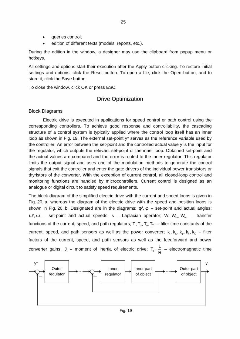
Electric drive is executed in applications for speed control or path control using the corresponding controllers. To achieve good response and controllability, the cascading structure of a control system is typically applied where the control loop itself has an inner loop as shown in Fig. 19. The external set-point y* serves as the reference variable used by the controller. An error between the set-point and the controlled actual value y is the input for the regulator, which outputs the relevant set-point of the inner loop. Obtained set-point and the actual values are compared and the error is routed to the inner regulator. This regulator limits the output signal and uses one of the modulation methods to generate the control signals that exit the controller and enter the gate drivers of the individual power transistors or thyristors of the converter. With the exception of current control, all closed-loop control and monitoring functions are handled by microcontrollers. Current control is designed as an analogue or digital circuit to satisfy speed requirements.
The block diagram of the simplified electric drive with the current and speed loops is given in Fig. 20, a, whereas the diagram of the electric drive with the speed and position loops is shown in Fig. 20, b. Designated are in the diagrams: , φ*φ – set-point and actual angles;
, ω*ω – set-point and actual speeds; s – Laplacian operator; , , ω ϕrrrI WWW – transfer
functions of the current, speed, and path regulators; CI TTTT , , , φω – filter time constants of the
current, speed, and path sensors as well as the power converter; CkI kkkkk , , , , φω – filter
factors of the current, speed, and path sensors as well as the feedforward and power
converter gains; J – moment of inertia of electric drive; RL
Te = – electromagnetic time
y* y
Fig. 19
Outer part of object
Inner part of object
Inner
regulator
Outer
regulator

26
constant; ω MMIm kkJRT = – mechanical time constant; M
MMI M
Ik = ,
M
MM E
kω
ω ≈ – motor torque and
speed constants; MMMM RIUE += – motor electromotive force (EMF), MC LLL += – control circuit
inductance including the inductances of converter and motor control winding; MC RRR += –
control circuit resistance including the resistances of converter and motor control winding. Index M marks the motor rated data: current, torque, speed, etc.
Parameters of the asynchronous electric drive having the stabilized rotor flax linkage are as follows:
1 LL σ= , 21 1σ kk−= , 1
121 L
Lk = ,
2
122 L
Lk = ,
314
23 12
12
XL ⋅= , 12
11 314
LX
L += , 122
2 314L
XL += ,
2221 RkRR +=
where index 1 designates the stator parameters and index 2 marks the rotor parameters,
1221211221 , , , , , , , LLLRRXXX are the rated values from the data tables.
The time constants of the filters ϕ ω , TTT ,I must be chosen as tiny as possible because they
restrict the dynamic response of the drive. If the time constant of the filter is too high, the system is slowed down and losses some of its dynamics.
ω* LM
CU
ω rW)1(
1+sTR e1+sT
k
C
C
1ω
ω
+sT
k
1+sT
k
I
I
IrW
ω
1
Mk
Js1
MIk1
φ rW )( 12 ++
ω
sTsTTi
k
mem
M 1+sT
k
C
C
1+ϕ
ϕ
sT
k1ω
ω
+sT
k
ω rW s1
φ* skk
I
ω φ
i1ω
а.
b
Fig. 20

27
In the case of absence of information, the feedback and converter factors and time constants can be accepted as follows: CI kkkk ω === ϕ = 1; ϕ= ω TT = 10 ms, IT = 10 ms for a thyristor
and 1 ms for a transistor converter; CT = 0…6 ms dependently on the converter type,
MIM kk =ω , L= 1…10 mH, R = 1…10 Ω.
When simulation in eDrive is processed, the program automatically identifies some missing data (resistances, inductances, torques, voltages, currents, and powers) and includes them into the calculated data chapter onto the Analysis tab of the Result window and into the report.
Tuning of the Current-Speed Loop System
Usually in the process of the current loop analysis, the EMF feedback is preliminary neglected. This feedback is shown by the dotted lines in the block diagram Fig 20, a. Then, the object of the simplified inner current loop is described by the transfer function
( ) ( )1 1 )(
µ ++=
sTsTRkk
sWeI
ICoI
where ICI TTT +=µ is a small time constant of the current loop. To control this object in
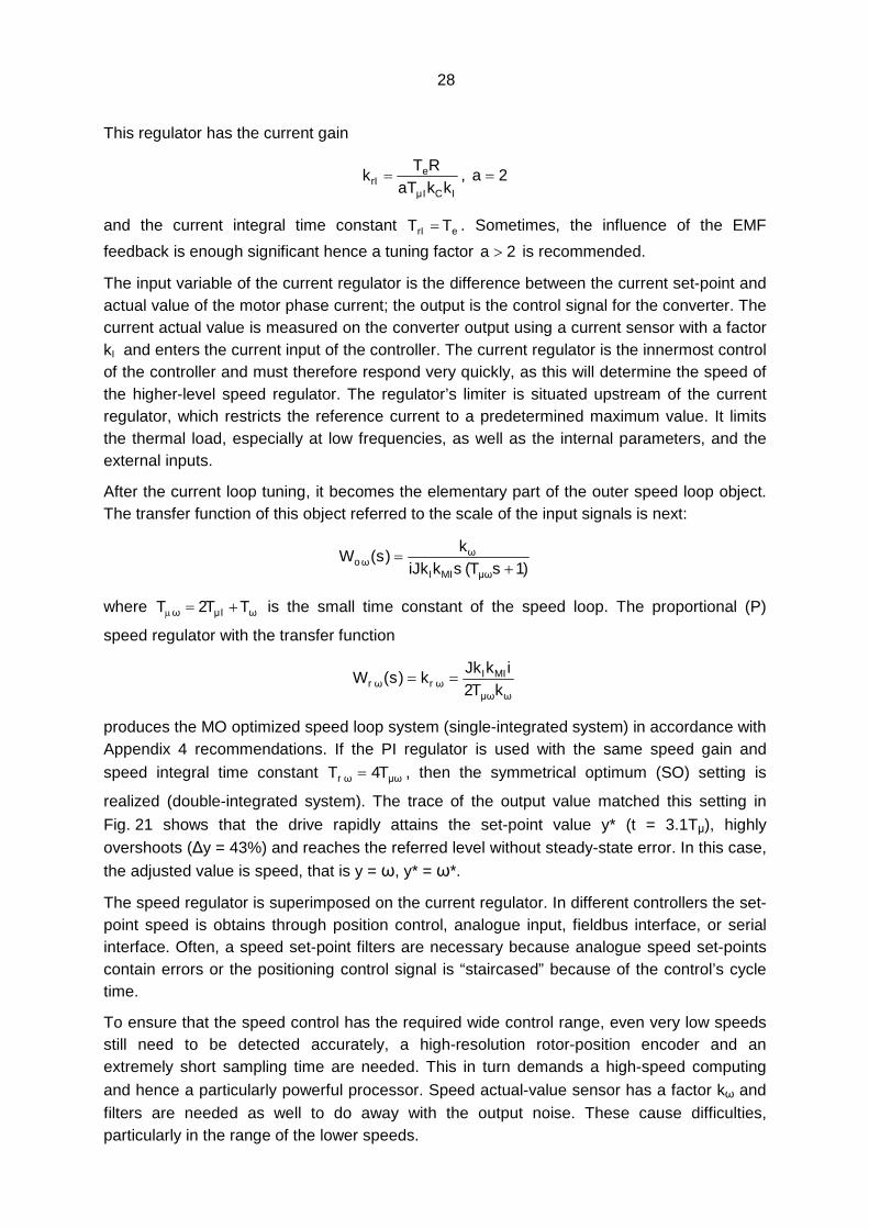
accordance with the cascading adjustment principle illustrated in Appendix 4, a proportional-integral (PI) regulator is commonly used with the modulus optimum (MO) setting. The trace of the output value y matched this setting is shown in Fig. 21 where the drive rapidly attains
the set-point value y* (t = 4.7Tµ), overshoots ones (∆y = 4.3%) and reaches the referred level with a small steady-state error. In the case of current loop, the adjusted value is the current, that is y = I, y* = I*. The transfer function of the current regulator is:
+=
sTksW
rIrIrI
11)( ,
0.43
Fig. 21
yyk
µTt
SO MO
0.043
3.1
4.7
1
28
This regulator has the current gain
ICI
erI kkaT
RTk
µ
= , 2=a
and the current integral time constant erI TT = . Sometimes, the influence of the EMF
feedback is enough significant hence a tuning factor 2>a is recommended.
The input variable of the current regulator is the difference between the current set-point and actual value of the motor phase current; the output is the control signal for the converter. The current actual value is measured on the converter output using a current sensor with a factor kI and enters the current input of the controller. The current regulator is the innermost control of the controller and must therefore respond very quickly, as this will determine the speed of the higher-level speed regulator. The regulator’s limiter is situated upstream of the current regulator, which restricts the reference current to a predetermined maximum value. It limits the thermal load, especially at low frequencies, as well as the internal parameters, and the external inputs.
After the current loop tuning, it becomes the elementary part of the outer speed loop object. The transfer function of this object referred to the scale of the input signals is next:
)1( )(
µω
ωω +
=sTskiJk
ksW
MIIo
where ωµω 2 TTT I +=µ is the small time constant of the speed loop. The proportional (P)
speed regulator with the transfer function
ωµω
ωω 2)(
kTikJk
ksW MIIrr ==
produces the MO optimized speed loop system (single-integrated system) in accordance with Appendix 4 recommendations. If the PI regulator is used with the same speed gain and
speed integral time constant µωω 4TTr = , then the symmetrical optimum (SO) setting is
realized (double-integrated system). The trace of the output value matched this setting in
Fig. 21 shows that the drive rapidly attains the set-point value y* (t = 3.1Tµ), highly overshoots (∆y = 43%) and reaches the referred level without steady-state error. In this case,
the adjusted value is speed, that is y = ω, y* = ω*.
The speed regulator is superimposed on the current regulator. In different controllers the set-point speed is obtains through position control, analogue input, fieldbus interface, or serial interface. Often, a speed set-point filters are necessary because analogue speed set-points contain errors or the positioning control signal is “staircased” because of the control’s cycle time.
To ensure that the speed control has the required wide control range, even very low speeds still need to be detected accurately, a high-resolution rotor-position encoder and an extremely short sampling time are needed. This in turn demands a high-speed computing
and hence a particularly powerful processor. Speed actual-value sensor has a factor kω and filters are needed as well to do away with the output noise. These cause difficulties, particularly in the range of the lower speeds.

29
Speed control can be executed with the speed limiting that restricts the set-point value to a maximum speed. If the drive reaches the permissible speed, it will stay at this speed and thus operates under the speed control. If the load is too great, the drive will reach the current limit before the motor attains the specific speed. If the load increases still further, the motor can come to a standstill and an error will be detected by the monitoring system.
Fig. 22 shows the step responses of the asynchronous open-ended electric drive and the closed loop drive. The second one has the stabilized rotor flax linkage and is optimized with a PI current restricted regulator and a P speed regulator. The response of the open-ended system depends on the input signal value: more the input, more the overshoot, response time, and steady-state error. Thanks to the MO setting, the run-up time becomes independent on the input level while the dynamic and the steady-state errors decrease without extra overshoot.
Fig. 23 shows a couple of step responses aroused by an instantly loaded dc thyristor electric drives. In Fig. 23, a, the open-ended system has the significant speed downfall due to the rectangle disturbance. On the contrary, Fig. 23, b illustrates the optimized closed loop system, which has no speed downfall from the same disturbance.
Tuning of the Speed-Path Loop System
The speed loop object shown in Fig. 20, b is described by the transfer function
)1)(1( )(
µω
ωωω +++
=sTsTTsTi
kkksW
mem
MCo 2
with the small time constant of the speed loop ωω TTT C +=µ .
In accordance with the cascading adjustment principle illustrated by the Appendix 4, different circuit settings are possible here. On the one hand, the MO setting guarantees the fast non-periodical control step response with a small speed error and with no steady-state disturbance error. At the same time, the setting of such kind droops the disturbances response and often results in the significant disturbance overshoot. The other way round, the SO setting gives the fast non-periodical disturbance response with no steady-state
Fig. 22

30
disturbance error and without the steady-state control error. In turn, this setting droops the control step response and results in the considerable control overshoot.
If the mechanical time constant is so low, that em TT 4≤ , then the proportional-integral-
differential (PID) regulator is recommended for the MO setting. Its transfer function is
++= sT
sTksW r
rrr 2ω
1ωωω )(
11 ,
the speed gain is equal
ωµω
ω kkTiJRk
kC
MIr 2
= ,
the speed integral time constant is mr TT =1ω , and the speed differential time constant is
er TT =2ω . The SO setting requires the more complex compensational regulator. In other
situations, the speed PID regulator is used, which equivalent time constants are as follows:
a.
Fig. 23
b.

31
2ω ,1ω rrT emmm TT
TT−
±=2
22.
Here, the MO setting is recommended with the speed gain
ωωµω
1ωω 2 kkkT
iTk
MC
rr = .
Nevertheless, when the condition Ie TT µ>> is not met, these formulae may be accepted as a
first approximation only.
In any case, the integral component makes sure that there is no steady-state error (i.g. under load). In most applications, to prevent possible overshoot the regulator’s D component is set to zero because of its difficult adjustment.
In this system, the input variable of the speed regulator is the difference between the speed set-point and actual measured value; the output is the control voltage for a modulator. The speed regulator is the innermost control of this controller and must therefore respond very quickly, as this will determine the speed of the higher-level path regulator. The regulator’s limiter is situated upstream of the speed regulator, which restricts the reference speed to a predetermined maximum value. Similar to the current regulator of the previous circuit, it limits the thermal load, especially at low frequencies, as well as the internal parameters, and the external inputs.
After tuning finishing, the optimized speed loop becomes the part of the external path loop object. The transfer function of this object with the optimized speed loop and referred input signals is equal
)ss(Tk
k(s)Wo 1µφω
φφ +
=
where the small path time constant is 2 φµωµφ TTT += .
The path control ensures a match between the currently measured positions with a target position by providing the motor with the appropriate values. The position data are usually obtained from a digital encoder. The path regulator with a transfer function
φµφ
ωφφ kT
kk(s)W rr 2
==
is implemented as pure proportional (P) regulator that provides the MO setting of the path loop. On the other hand, to accomplish the SO setting, the path PI regulator is required with
the same path gain and the path time constant µφφ 4TTr = . Nevertheless, an integral
component would result in impermissible overshoot when the target position is approached.
Often, the path P regulator with the feedforward gain φ
ω
2kk
kk = is used instead of the PI
regulator. The feedforward is connected in parallel with the path regulator to better control the steady-state process. The path set-point is routed to a differential circuit, which output magnitude depends on the speed timing fluctuations and on the feedforward gain. Since the

32
feedforward is effective only within a certain range, it often takes a turn for the worse of the system’s control response and the disturbance response.
System Jog
During the regulators’ calculation, a lot of assumptions have been carried out. If you are not satisfied with the results obtained, the jog operation is required resulting in the gains and time constants supplemental adjustment. The closed-loop drive simulation lets to evaluate the system response on the step input and disturbances as well as on the non-step inputs. As a rule, permissible and approvable drive outputs meet such requirements as:
• approaching the set-point speed and path;
• almost rated steady torque, current, power, and voltage; • transient overtorque and overcurrent according to the data table restrictions or, if
absent, 150 to 200 % of the rated values for 0.2 to 10 s.
If the regulator calculation gives poor results, then the regulator gains and time constants need to find more exact or tune the system again.
The jog of the loops in the cascading control systems is executed step by step, beginning from the inner loop. Firstly, a P regulator is included into a loop and small inputs and disturbances enter the system without the capturing. In these conditions, the transients and steady processes are investigated with smoothly rising of the system gain. Increasing this value enhances the response but a too high value will make the system liable to vibrate. As the closed-loop gain raises, the transient time reduces but the overshoot and the steady-state ripple increase. Therefore, increase the gain within the vibration- and unusual noise-free range, and return slightly if oscillation takes place.
To eliminate stationary deviation against a reference, the control loop provides with the integral control. For the integral compensation, firstly set an integral time constant enough high. Decreasing this setting raises the response level. However, if the load moment of inertia is large or the mechanical system has any vibratory element, the driving system is liable to vibrate unless the setting is increased to some degree. Therefore, decrease smoothly the integral time constant within the vibration-free range, and return slightly if vibration takes place.
If the loop response remains low, the differential control may be added. Initially, set a differential time constant low. Smoothly rising its value, look for the overshoot and vibration. When their level becomes dangerous, return slightly the differential time constant.
Start the current loop jog without the speed and path loops. Then, continue the speed jog using the working load without the path loop. When both inner loops will be ready, tune the path loop, firstly without the predictive loop. Then, raise slightly the feedforward gain of the feedforward loop, which compensates the steady-state speed error.
While checking the transient and steady characteristics and rotational status, fine adjust each gain for getting the required transient time, overshoot, and precision. After the linear system jog finishing, include the regulators’ limiters and increase the input signals. By such a way, check the drive response of the constrained system. When the acceleration start-up level is to be restricted, limit the current or the input ramp. Thus, a reduction in the start-up

33
acceleration and braking deceleration and consequently a smoother start-up and deceleration can be achieved by soft start/brake.

34
Appendixes
1. Model Arrangement
It is of major importance, that an effective model has to enclose some structural and information redundancy to take account of future progress of the simulating object. That is why a generalized objects description is the best tool for the model base classes design. It applies an inheritance of new modules without any deconstruction of the main model structure. The eDrive software is the real example of the object-oriented technology implementation.
In the software, the integration of the large variety of models has been carried. As a result, the generalized electric machine description became the base of electric motor’s model of well-known and possible unknown types. By analogy, the generalized discrete converter description has been used as the base of power converter model of known and unknown types. In the load model, the efforts have been directed towards the choice and linking the traditional models of gears, couplings, and transmissions.
The developed class library comes up to ANSI standards and contains four base classes, shown in Fig. 24:
• the electric motors class, • the power electronic converters class,
• the mechanical gears and loads class,
• the result representation class.
The class Motor joins private data members that store information of the number of calculating points, the model time steps, and the elastic deformation period of mechanical part of the system. Moreover, it has the private functions that represent the generalized two-phases electric motor’s model, which variables are stator and rotor phase currents, electromagnetic torques, and rotation speeds of rotor field and loading shaft. Protected variables of the class Motor describe the type of power converter and load, the motor poles number, phases number, inductance and resistance, moment of inertia, electromechanical and electromagnetic factors. Protected member-functions list includes motor parameter functions that implement the procedure for solution of the differential equations. Any free
base class Trans
base class Loads
base class Graph
derived class DCEX
derived class
DCPM
derived class ACSC
derived class VM
Base class Motor
Fig. 24

35
model element may interconnect with the private and protected members via the public functions that move results into the file or onto the display screen.
The class DCEX has been inherited from Motor. It is the model of a dc motor with an excitation circuit. Its members control the data entering for the computation process. Other inherited classes DCPM (dc motor with permanent magnets), ACSC (squirrel-cage induction motor), and VM (synchronous motor) have the same structure.
The next base class Trans describes power supplies of different kinds for the motors of the class Motor. Motor has been announced as a friend class for the Trans, so it has got an access into the private area of Trans. Trans encapsulates the private variables that describe the type of power supply, and some private methods. They supervise the choice of an appropriate power source and describe the three-phase and dc supply mains with their inductance and resistance. Some polymorphous functions reflect the nature of thyristor converters and transistor modulators. The public variables of the class Trans store information about frequency, voltage, resistance, and inductance of power converters as well as connect the class with other eDrive modules.
The base class Loads includes the mechanisms' models of different kinds. Its private area encloses such data members as load type, load torque, elastic and tough factors, etc. The dispatch functions simulate constant and time-change loads. The public area of this class includes moment of inertia and gear description. The class Motor is announced as a friend of Loads.
The last base class Graph consists of two parts. Its private data members are scale factors and extreme values. Its private functions are the diagram scaling parameters. Among the public member-functions one can find the static diagram building machine, the dynamic diagram generator, and the result analyzer.
2. Navigation and Data Edition
When you need the eDrive data entering or edition, click a field or tab and place the mouse pointer there. Another method of pointer moving is to use the hotkeys:
next field TAB previous field SHIFT+TAB. next tab RIGHT ARRAY KEY previous tab LEFT ARRAY KEY next character RIGHT ARRAY KEY or DOWN ARRAY KEY previous character LEFT ARRAY KEY or UP ARRAY KEY end of line END start of line HOME
Use the auxiliary hotkeys for traveling along the tab Editor in Connections window:
next word CTRL+ RIGHT ARRAY KEY previous word CTRL+ LEFT ARRAY KEY next paragraph CTRL+ DOWN ARRAY KEY previous paragraph CTRL+ UP ARRAY KEY next line DOWN ARRAY KEY previous line UP ARRAY KEY

36
next screen PAGE DOWN or CTRL+PAGE DOWN previous screen PAGE UP or CTRL+PAGE UP end of document CTRL+END start of document CTRL+HOME
Functional keys:
Help F1 Window Result F5 Window Model F6 Window Database F7 Window Connections F8 Selection menu F10
To mark a text, drag the mouse pointer along it. To mark a word, double click it. To extend selection, use next hotkeys:
character right SHIFT+ RIGHT ARRAY KEY character left SHIFT+ LEFT ARRAY KEY to the end of word CTRL+SHIFT+ RIGHT ARRAY KEY to the start of word CTRL+SHIFT+ LEFT ARRAY KEY to the end of line SHIFT+END to the start of line SHIFT+HOME
Use the auxiliary hotkeys to extend selection on the tab Editor in Connections window:
next line SHIFT+ DOWN ARRAY KEY previous line SHIFT+ UP ARRAY KEY to the end of paragraph CTRL+SHIFT+ DOWN ARRAY KEY to the start of paragraph CTRL+SHIFT+ UP ARRAY KEY next screen SHIFT+PAGE DOWN previous screen SHIFT+PAGE UP to the end of text CTRL+SHIFT+END to the start of text CTRL+SHIFT+HOME
To delete data use next keys:
deleting left character BACKSPACE deleting right character DEL deleting to the clipboard SHIFT+DEL cancellation of operation CTRL+Z
Both operations begin from marking a text, which is meant for moving or copying. Then:
select menu Cut (SHIFT+DEL) for moving; select menu Copy (CTRL+INS) for copying; place the pointer to inserting position and use menu Paste (SHIFT+INS).
3. Database fields names
Converter converter type Pc_W converter power, W Uc_V converter phase voltage, V

37
Ic_A converter current, A Icm_A converter maximum current, A Fcm_Hz converter maximum frequency, Hz L1c_mH, L2c_mH converter inductance, mH R1c_Ohm, R2c_Ohm converter resistance, Ohm mc converter number of pulses per supply voltage period masc_kg converter mass, kg Gear gear type Pg_W gear power, W Mg_Nm gear torque, Nm ng_rpm gear input speed, rpm Ig gear ratio %g gear efficiency, % masg_kg gear mass, kg
Jg_kgcm2 gear moment of inertia, kg⋅cm2 vg_cms gear screw-nut velocity, cm/s rg_cm gear screw radius, cm Motor motor type P_W motor power, W M_Nm motor torque, Nm Mm_Nm motor maximum torque, Nm Ms_Nm motor stall torque, Nm n_rpm motor angular speed. Rpm U_V motor voltage, V I_A motor current, A Is_A motor startup current, A R1_Ohm stator active resistance, Ohm X1_Ohm stator reactance, Ohm L1_mH stator inductance, mH R2_Ohm rotor active resistance, Ohm X2_Ohm rotor reactance, Ohm L2_mH rotor inductance, mH X12_Ohm exciting reactance, Ohm s induction motor slip sk induction motor critical slip
J_kgcm2 rotor moment of inertia. kg⋅cm2 % motor efficiency, % cos induction motor power factor, % mas_kg motor mass, kg

38
4. Regulators for Typical Objects
Object model Conditions Opti-mum
Regu-lator
Gains and time constants
1+sTk
o
o — — PI o
or kT
Tk
µ
= , or TT =
MO P o
or kT
Tk
µ2=
)1( µ +sTsTk
o
o µ4TTo >
SO PI o
or kT
Tk
µ2= , µ4TTr =
MO PI o
or kT
Tk
µ2= , or TT =
)1)(1( µ ++ sTsTk
o
o µ4TTo >
SO PI o
or kT
Tk
µ2= , µ4TTr =
MO I o
r kTT
µ21
=
1µ +sTko —
SO I o
r kTT
µ
4=
MO PID o
or kT
Tk
µ
1
2= , 11 or TT = ,
22 or TT =
)1)(1( 12
21µ +++ sTsTTsT
k
ooo
o 21
µ1
4
16
oo
o
TT
TT
≤
>
SO Com-
pensa-tional
o
or kT
Tk
µ
1
2= , 1or TT =1 ,
22 or TT = , µ3 4TTr =
MO PID o
or kT
Tk
µ
1
2
′= , 11 or TT ′= ,
22 or TT ′=
)1)(1)(1( 21µ +′+′+ sTsTsTk
oo
o 1µ
2µ4
o
o
TT
TT
′≤
′>
4
SO PID o
or kT
Tk
µ
1
2
′= , µ1 4TTr = ,
22 or TT ′=
MO PID o
or kT
Tk
µ
1
2
′= , 11 or TT ′= ,
22 or TT ′=
12
µ2 4
oo
o
TT
TT
′<′
≥′
SO PID o
oor kT
TTk
2µ
21
8
′′= , 21 or TT ′= ,
µ2 4TTr =

39
References on Simulation Instruments
1. Attia, J. O. , PSpice and Matlab for Electronics: An Integrated Approach, Boca Raton (FL) [etc.]: CRC Press, 2002. 338 p. ISBN: 0849312639
2. Berube, R. H. , Computer Simulated Experiments for Electric Circuits Using Electronics Workbench, Upper Saddle River (NJ); Columbus (OH): Prentice Hall, 1997. 263 p. ISBN: 0133596214
3. Borris, J. P. , Semiconductor Devices Simulation Using Electronics Workbench, Upper Saddle River (NJ); Columbus (OH): Prentice-Hall, 2000. 207 p. ISBN: 0130260835
4. Craig, E. C. , Laboratory Manual for Electronics via Waveform Analysis, New York [etc.]: Springer, 1994. 130 p. ISBN: 0387941363
5. Gosling, J. B. , Simulation in the Design of Digital Electronic Systems, Cambridge [etc.]: Cambridge University Press, 1993. 273 p. ISBN: 0521426723
6. Horsey, M. P. , Electronics Projects Using Electronics Workbench, Oxford [etc.] : Newnes, 1998. 227 p. ISBN: 0750631376
7. Kularatna, N. , Power Electronics Design Handbook, Boston: Newnes, 1998. 300 p. ISBN: 0750670738
8. Lenk, J. D. , Simplified Design of Switching Power Supplies, Boston: Butterworth-Heinemann, 1995. 224 p. ISBN: 0750695072
9. Massobrio, G. , Semiconductor Device Modeling with Spice, New York: McGraw-Hill, 1993. 479 p. ISBN: 0070024693
10. Price, T. E. , Analog Electronics: An Integrated PSpice Approach, London [etc.]: Prentice hall, 1997. 706 p. ISBN: 0132428431
11. PSpice Reference Guide , Oregon: Cadence PCB System Division. 2000
12. PSpice User’s Guide , Oregon: Cadence PCB System Division. 2000
13. Raghuram, R. , Computer Simulation of Electronic Circuits, New York [etc.]: New Delhi: Wiley; Wiley Eastern, 1989. 246 p. ISBN: 0470213310
14. Ramshaw, R. and D. Schuurman , PSpice Simulation of Power Electronic Circuits, An Introductory Guide, NY: Chapman & Hall, 1996. 400 p. ISBN: 0412751402
15. Tuinenga, P. W. , Spice: A Guide to Circuit Simulation and Analysis Using PSpice, Englewood Cliffs (NJ): Prentice Hall, 1995. 288 p. ISBN: 0134360494
16. Vodovozov, V. M. and R. Jansikene , Power Electronic Converters, Tallinn: TUT, 2006. 120 p. ISBN: 9985690389
17. Болотовский, Ю. И., Г. Таназлы, OrCAD. Моделирование. “Поваренная книга”, Москва: Солон-Пресс. 2005
18. Водовозов, В. М., Проектирование электропривода с использованием пакета eDrive, СПб: Изд-во СПбГЭТУ “ЛЭТИ”, 2006, 32 с.

40
19. Карлащук, В. И., Электронная лаборатория на IBM PC: Программа Electronics Workbench и ее применение, Москва: Солон-Р, 1999. 70 с. ISBN: 5934550063
20. Панфилов, Д. И., В. С. Иванов, И. Н. Чепурин, Электротехника и электроника в экспериментах и упражнениях: Практикум на Electronics Workbench: В 2 т. Т. 1: Электротехника, Москва: Додэка, 1999. 304 с. Т. 2: Электроника, Москва: Додэка, 2000. 288 с. ISBN: 5878350513
21. Разевиг, В. Д., Система сквозного проектирования электронных устройств DesignLab 8.0, Москва: Солон. 1999.