of in-core fuel management of
TRANSCRIPT

MITNE-144
INCREMENTAL COSTS AND OPTIMIZATION
OF IN-CORE FUEL MANAGEMENT OF
NUCLEAR POWER PLANTS
Hing Yan Watt
MansonEdward
BenedictA. Mason
Department of Nuclear Engineering
Massachusetts Institute of Technology
Cambridge, Massachusetts
iwmwahw w ---- .. ..... .. ......... ..

MITNE-144
INCREMENTAL COSTS AND OPTIMIZATION OF IN-CORE
FUEL MANAGEMENT OF NUCLEAR POWER PLANTS
by
Hing Yan Watt
Supervisors
Manson BenedictEdward A. Mason
DEPARTMENT OF NUCLEAR ENGINEERING
MASSACHUSETTS INSTITUTE OF TECHNOLOGY
CAMBRIDGE, MASSACHUSETTS
Issued: February 1973

2
INCREMENTAL COST AND
NUCLEAR IN-CORE OPTIMIZATION
by
Hing Yan Watt
Submitted to the Department of Nuclear Engineeringon January 17, 1973 in partial fulfillment of the require-ment for the degree of Doctor of Science.
ABSTRACT
This thesis is concerned with development of methodsfor optimizing the energy production and refuelling decisionfor nuclear power plants in an electric utility systemcontaining both nuclear and fossil-fuelled stations. Theobjective is to minimize the revenue requirements forrefuelling the power plants during the planning horizon; thedecision variables are the energy generation, reloadenrichment and batch fraction for each reactor cycle; theconstraints are that the customer's load demand, as wellas various other operational and engineering requirementsbe satisfied. This problem can be decomposed into twosub-problems. The first sub-problem is concerned withscheduling energy between nuclear reactors which havebeen fuelled in an optimal fashion. The second sub-problemis concerned with optimizing the fuelling of nuclear reactorsgiven an optimized energy schedule. These two sub-problemswhen solved iteratively and interactively, would yield anoptimal solution to the original problem.
The problem of optimal energy scheduling betweennuclear reactors can be formulated as a linear program. Theincremental cost of energy is required as input to the linearprogram. Three methods of calculating incremental cost areconsidered: the Rigorous Method, based on the definitionof partial derivativesis accurate but time consuring; theInventory Value Method and the Linearization Method, basedrespectively on equations of inventory evaluation andlinearization, are less accurate, but efficient. The lattertwo methods are recommended for the early stages of optimiza-tion.
The problem of optimizing the fuelling of nuclearreactors has been solved for two cases: the special caseof steady state operation, and the general case of non-steady-state operation. The steady-state case has beensolved by simple graphic techniques. The results indicate

3
that reactors should be refuelled with as small a batchfraction as allowed by burnup constraints. The non-steadycase has been solved by polynomial approximation, in whichthe objective function as well as the constraints areapproximated by a sum of polynomials. The results indicatethat the final selection of an optimal solution from a setof sub-optimal solutions is primarily based on engineeringconsiderations, and not on economics considerations.
Thesis Supervisors: Manson BenedictInstitute Professor
Edward A. MasonDepartment Head and Professor of
Nuclear Engineering

U
LIST OF CONTENTS
Chapter Page
Abstract 2List of Contents 4List of Tables 8List of Figures 12Acknowledgement 14
1 SUMMARY AND CONCLUSIONS 15
1.1 Framework for Analysing the Overall 15Optimization Problem of Mid-RangeUtility Planning
1.2 Optimal Energy Scheduling between 20Two Pressurized Water Reactors ofDifferent Sizes Operating in SteadyState Conditions
1.3 Calculation of Objective Function 23for Non-Steady State Operations
1.4 Calculation of Incremental Cost of 28Nuclear Energy Aand Reload En-richments for a Given Set of RequiredEnergies and for Fixed Reload Batch Frac-tion1.4.1 Rigorous Method1.4.2 Inventory Value Method1.4.3 Linear Approximation Method
1.5 Calculation of Incremental Cost and 36Nuclear In-Core Optimization forReactors Operating Under Steady-StateConditions
1.6 Test of Objective Function for the 44Variable Batch Fraction, Non-SteadyState Case
1.7 The Method of Piece-Wise Linear 48Approximation for the Problem ofNuclear In-Core Optimization
1.8 The Method of Polynomial Approxima- 52tion for the Problem of NuclearIn-Core Optimization
1.9 Conclusions 591.10 Recommendations 65
2 INTRODUCTION 67
2.1 Motivations for Mid-Range Utility 67Planning
2.2 Formulation of the Overall Optimiza- 69tion Problem for Mid Range UtilityPlanning

5
2.3 Decomposition of the Overall Problem 71into Various Sub-Problems
2.4 Brief Description of the Solution 75Technique for the Problem of OptimalEnergy Scheduling
2.5 The Organization of the General and 78Special Problem of Nuclear In-CoreOptimization
2.6 Types of Reactors Analyzed 792.7 Depletion Code CELL-CORE 812.8 Economics Code MITCOST1 and COCO 82
3 OPTIMAL ENERGY SCHEDULING FOR STEADY-STATE 83OPERATION WITH FIXED RELOAD BATCH FRACTIONSAND SHUFFLING PATTERN
3.1 Defining the Problem 833.2 Defining the Objective Function 843.3 Defining the Dacision Variables and 85
the Design Variables3.4 Lagrangian Optimality Condition 853.5 The Optimization Procedures 87a3.6 Summary and Conclusions 96
4 OBJECTIVE FUNCTION FOR NON-STEADY STATE CASES 98
4.1 Introduction 984.2 Objective Function Defined for the Case 99
With No Income Tax4.2.1 Formulating the Problem4.2.2 The Condition of Consistency4.2.3 The Condition of Equalized
Incremental Cost4.3 Three Methods of Evaluating Fuel Inventories 103
4.3.1 Nuclide Value Method4.3.2 Unit Production Method4.3.3 Constant Value Method
4.4 Results of Two Sample Cases 1054.5 Objective Function Defined for the 112
Case With Income Tax4.5.1 Objective Function for the Indefinite
Time Horizon4.5.2 Objective Function for the Finite
Time Horizon4.5.3 Conditions of Consistency and
Equalized Incremental Cost b4.6 Two Methods of Evaluating Fuel Inventories V 1154.6.1 Inventory Value Method4.6.2 Unit Production Method
4.7 Results of Two Sample Cases 1184.8 Conclusions 120

5 CALCULATION OF RELOAD ENRICHMENT AND INCREMENTAL 122COST OF ENERGY FOR GIVEN SCHEDULE OF ENERGYPRODUCTION WITH FIXED RELOAD BATCH FRACTION ANDSHUFFLING PATTERN
5.1 Defining the Problem 1225.2 One-Zone Refuelling 123
5.3 Multi-Zone R'efuelling 1255.3.1 The Rigorous Method5.3.2 Linearization Method5.3.3 Inventory Value Method
5.4 Results For Three Sample Cases 134
5.4.1 Sample Case 1 & 25.4.2 Sample Problem 3
5.5 Conclusions 140
6 CALCULATION OF OPTIMAL RELOAD ENRICHMENT AND 144RELOAD BATCH FRACTION FOR REACTORS OPERATINGIN STEADY STATE CONDITION AND MODIFIED SCATTERREFUELLING
6.1 Introduction 1446.2 Mathematical Formulation of the Problem 144
and Optimality Conditions6.3 Graphic Solution for Optimal Batch 147
Fraction6.4 Interpretation of the Lagrangian 150
Multiplier 7r6.5 Calculation of Incremental Cost 153
of Energy X6.6 Effects of Shortening the Irradiation 157
Interval6.7 Conclusions 157
7 NUCLEAR IN-CORE OPTIMIZATION FOR NON-STEADY 169STATE.FORMULATION OF THE PROBLEM
7.1 Introduction 1697.2 Mathematical Formulation of the Problem 170
7.3 Exact and Approximate Calculation of the 173Objective Function
7.4 Comparison of the Exact and Approximate 176Methods
1837.5 Conclusions
7
8 NUCLEAR IN-CORE OPTIMIZATION FOR NON-STEADY 184STATE BY METHOD OF PIECE-WISE LINEAR APPROXIMATION
8.1 Introduction 1848.2 The Optimization Algorithm 1848.3 Results for Sample Case A 190
with No Income Tax8.4 Results for Sample Case A 195
with Income Tax8.5 Conclusions 195
9 NUCLEAR IN-CORE OPTIMIZATION FOR NON-STEADY 198STATE BY METHOD OF POLYNOMIAL APPROXIMATION
9.1 Introduction 1989.2 Brief Comments about the Objective 199
Function and the End Conditions9.3 Choice of the Polynomials 2019.4 Regression Analysis on Objective Function 2129.5 Optimization Algorithm 2159.6 Results of Sample Case A and B 219
9.7 Estimates of Burnup Penal'ty IT 2309.8 Incremental Cost 2319.9 Summary and Conclusions 235
10 CONCLUSIONS AND RECOMMENDATION 239
10.1 Conclusions 23910.2 Recommendation 240
Biographical Note 242
Appendix A Brief Description of the Several Versions of CORE 243
Appendix B Economics and Fuel Cycle Cost Parameters 244
Appendix C Nomenclature 246
Appendix D List of References 250

8
LIST OF TABLES
Page
1.1 Comparison of Exact Incremental Cost with 27Incremental Cost Calculated by Two ApproximateMethods
1.2 Incremental Cost of Energy Calculated by 33Three Methods (Rigorous Method, LinearizationMethod and Inventory Value Method)
1.3 Reload Enrichments Calculated by (1) Trial 35Method (2) Linearization Method
1.4 Effect of Variation of Enrichment and Batch 47Fraction on Revenue Requirement
1.5 Reload Enrichments, Batch Fractions, Cycle 51Energies and Revenue Reauirements forVarious Number of Iterations Using the Methodof Piece-Wise Linear Approximation
1.6 Reload Enrichments, Batch Fractions, Cycle 54Energies and Revenue Requirements for theVarious Lowest Cost Cases Using the Methodof Polynomial Approximation on Sample Case A
1.7 Average Discharge Burnup for the Sublot 55Experiencing the Highest Exposure for SampleCase A Calculated by (1) Polynomial Approxi-mation Based on Regression Equations (2)CELL-CORE Depletion Calculation
1.8 Reload Enrichments for the Various Lowest 56Cost Cases Using the Method of PolynomialApproximation
1.9 Average Discharge Burnup for the Sublot 58Experiencing the Highest Exposure forSample Case B Calculated by (1); PolynomialApproximation Based on Regression Equations(2) CELL-CORE Depletion Calculation
1.10 Calculation of Incremental Cost of Energy 60Using Regression Equations. Sample CaseA for Burnup Limit B'= 45MWD/Kg
1.11 Calculation of Incremental Cost of Energy 61Using Regression Equations. Sample CaseA for Burnup Limit B* = 50M WD/Kg

9
1.12 Calculation of Incremental Cost of Energy 62Using Regression Equations. Sample CaseB for Burnup Limit B* = 45MWD/Kg
1.13 Calculation of Incremental Cost of Energy 63Using Regression Equations. Sample CaseB for Burnup Limit B = 50MWD/Kg
2.1 Various Steps in the Decomposition of the 76Overall Optimization Problem of Mid-RangeUtility Planning
2.2 %ontents n' tCe a chapters in This 80Thesis
3.1 Cycle Energy and Revenue Requirement for 88Different Enrichments
4.1 Feed Enrichment and Energy Per Cycle for 106Steady State Case and the Two Perturbed Cases
4.2 Comparison of Exact Incremental Cost with 109Incremental Cost Calculated by Three Approxi-mate Methods (No Income Tax)
4.3 Test of Inconsistency between the Exact Value 119and the Approximate Methods
4.4 Comparison of Exact Incremental Cost with 121Incremental Cost Calculated by Two Approxi-mate Methods
5.1 Refuelling Schedule (in years) 123
5.2 Incremental Cost of Energy for Sample Cases 1371 and 2 Calculated by Three Different Methods
5.3 Calculation ofIncremental Cost Using the 138Method of Linearization for Sample Case 1and 2
5.4 Reload Enrichment Salculated by Trial Method 139and by Linearization Method
5.5 Incremental Cost of Energy for Sample Case 1413 Calculated by Three Different Methods
5.6 Calculation of Incremental Cost Using the 142Method of Linearization for Sample Case 3
5.7 Reload Enrichment Calculated by the Trial 143Method and by the Linearization Method

10
6.1 Table of Revenue Requirement Per Cycle, Energy 148Per Cycle and Average Discharge Burnup versusBatch Fraction and Reload Enrichment
7.1 Exact and Approximate Revenue Requirement 178for Various Enrichments and Batch Fractions
7.2 Exact and Approximate Revenue Requirement 182Calculated for the Base Case and the Case inwhich the Reload Enrichments and BatchFractions for All the Cycles are Changed
8.1 Reload Enrichments, Batch Fractions, Cycle 193Energies and Revenue Requirements forVarious Number of Iterations Using the Methodof Piece-Wise Linear Approximation
8.2 Average Discharge Burnup for the Sublot 194Experiencing the Highest Exposure for SampleCase A Calculated by(1) Piece-Wise Linear Approximation(2) CELL-CORE Depletion Calculation
8.3 Reload Enrichments, Batch Fractions, Cycle 196Energies and Revenue Requirements withIncome Taxes for Various Number of It-erations Using the Method of Piece-WiseLinear Approximation
9.1 Regression Equation for Revenue Requirement 204
9.2 Regression Equation for Enrichment for Cycle 1 205
9.3 Regression Equation for Enrichment for Cycle 2 206
9.4 Regression Equation for Enrichment for Cycle 3 207
9.5 Regression Equation for Enrichment for Cycle 4 208
9.6 Regression Equation for Enrichment for Cycle 5 209
9.7 Reload Enrichments, Batch Fractions, Cycle 220Energies and Revenue Requirements for theVarious Lowest Cost Cases Using the Methodof Polynomial Approximation Sample Case A
9.8 Average Discharge Burnup for the Sublot Exper- 221iencing the Highest Exposure for Sample Case ACalculated by (1) Polynomial Approximation Basedon Regression Equations (2) CELL-CORE DepletionCalculation

11
9.9 Reload Enrichments, Batch Fractions, Cycle 223Energies and Revenue Requirements for theVarious Lowest Cost Cases Using the Methodof Polynomial Approximation. Sample Case A
9.10 Average Discharge Burnup for the Sublot 224Experiencing the Highest Exposure for SampleCase A Calculated by (1) Polynomial Approxi-mation Based on Regression Equations (2)CELL-CORE Depletion Calculation
9.11 Reload Enrichments, Batch Fractions, Cycle 226Energies and Revenue Requirements for theVarious Lowest Cost Cases Using the Methodof Polynomial Approximation.Sample Case B
9.12 Average Discharge Burnup for the Sublot 227Experiencing the Highest Exposure for SampleCase B Calculated by (1) Polynomial Approxi-mation Based on Regression Equations (2)CELL-CORE Depletion Calculation
9.13 Reload Enrichments, Batch Fractions, Cycle 228Energies and Revenue Requirements for theVarious Lowest Cost Cases Using the Methodof Polynomial Approximation.Sample Case B
9.14 Average Discharge Burnup for the Sublot 229Experiencing the Highest Exposure for SampleCase B Calculated by (1) Polynomial Approxi-mation Based on Regression Equations (2)CELL-CORE Depletion Calculation
9.15 Calculation of Incremental Cost of Energy 233Using Regression Equations.Sample Case A
9.16 Calculation of Incremental Cost of Energy 234Using Regression EquationsSample Case A
9.17 Calculation of Incremental Cost of Energy 236Using Regression Equations.Sample Case B
9.18 Calculation of Incremental Cost of Energy 237Using Regression Equations.Sample Case B

12
List of Figures
1.1 Incremental Cost vs Cycle Energy 211.2 Nuclear Sub-System Incremental Cost vs Total 22
Nuclear Energy Production1.3 Reload Enrichment vs Cycle Energy 241.4 Relationship Between the Various Revenue 32
Requirements Batch Number and Cycle Number1.5 Revenue Requirement vs Cycle Energy for 37
Various Batch Fractions1.6 Revenue Requirement vs Batch Fraction for 39
Different Levels of Energy1.7 Optimal Batch Fraction vs Cycle Energy for 40
Various Burnup Limits BO1.8 Revenue Requirement vs Reload Enrichment for 41
Various Levels of Energy1.9 Incremental Cost X vs Cycle Energy E for 43
Various Burnup Limit BO
3.1 Revenue Requirement R vs Cycle Energy EA 893.2 Revenue Requirement R vs Cycle Energy E5s 903.3 Incremental Cost dRss sdEss vs Cycle Energy 913.4 Nuclear Sub-System Incremental Cost vs 93
Total Nuclear Energy Production3.5 Reactor Energy vs Total Nuclear Energy 943.6 Reactor Capacity Factor vs Total Nuclear 95
Energy3.7 Reload Enrichment vs Cycle Energy 97
4.1 Relationships Between the Various Revenue 108Requirements Batch Number and Cycle Numbers
5.1 Cycle Energy vs Reload Enrichment for One- 124Zone Case
5.2 Revenue Requirement per Batch vs Cycle Energy 126for Five Succeeding Cycles
5.3 Incremental Cost vs Cycle Energy for 127Five Succeeding Cycles
5.4 Relationships Between the Various Revenue 135Requirements Batch Numbers and Cycle Numbers
6.1 Revenue Requirement vs Cycle Energy for 149Various Batch Fractions
6.2 Revenue Requirement vs Batch Fraction for 151Different Levels of Energy
6.3 Revenue Requirement vs Reload Enrichment for 152Various Levels of Energy
6.4 Incremental Cost X vs Cycle Energy for Various 156Burnup Limits B*
6.5 Objective Function TC vs Cycle Energy for 158Various Batch Fraction
6.6 Revenue Requirement vs. Batch Fraction for 159Different Levels of Energy

13
7.1 Relationships between the Various Revenue 174Requirements Batch Number and CycleNumber
7.2 Variation of TC1 and TCU with Respect 179to El
7.3 Variation of TC and TC with respect 180to Batch Fractibn fw r
8.1 Flow Chart for Method of Linear 187Approximation
8.2 Relationships Between TC, Batch and Cycle 192
9.1 Relationships Between Revenue Requirement, 200Batch Number and Cycle Number
9.2 Standard Estimate of Error in Enrichment 211Regression Egauations
9.3 Total Cost TC vs Cycle Energy E1 for 213Various Batch Fractions fl
9.4 Total Cost TC vs Batch Fraction for 214First Cycle fl for Different Energy E
9.5 Variation of TC with Respect to f, 216for Various f2 Holding f3 = f4 = f5 = 0.33
9.6 Optimization Algorithm 218

ACKNOWLEDGMENT 14
The author expresses his most grateful appreciation
to his thesis supervisors, Professor Manson Benedict and
Professor Edward A. Mason for the advice and guidance
throughout the course of this work.
The author would like to thank the Nuclear Engineering
Department at M.I.T. for offering teaching assistantships
and research assistantships throughout the three and half
yearsof his graduate study, and Commonwealth Edison Company
for supporting this thesis research.
The author would also like to thank Joseph P.Kearney,
Paul F. Deaton and Terrance Rieck for the many fruitful
discussions during the course of this work.
The author is grateful to the typist, Miss Linda Wildman
for her effort in the preparation of this manuscript.
Finally, the author would like to express his sincere
gratitude towards his parents and wife, An-Wen for their help,
understanding and love throughout his graduate school life,

CHAPTER 1.0SUMMARY AND CONCLUSIONS
151.1 Framework for Analyzing the Overall
Optimization Problems of Mid-Range Utility Planning
This thesis is concerned with development of methods
for optimizing the energy production and refuelling decision
for nuclear power plants in an electric utility system
containing both nuclear and fossil-fueled stations. The
time period under consideration is the so-called mid-range
period from five to ten years, within which nuclear fuel
management can be varied, for available nuclear plants.
The overall optimization problem of mid-range utility
planning can be formulated as follows: given a load forecast
for a given electric utility over the span of the planning
horizon, given the composition of the electric utility in
terms of the capacity, type and location of each generating
unit, find the optimal schedule of operation in terms of
energy produced by each plant and the reload enrichments and
batch fractions for each nuclear plant such that the revenue
requirements are minimized and the system constraints and
demands are satisfied. The revenue requirement is chosen as
the objective function, because it is favored by many electric
utilities (CEl, AEP1) and is relatively simple to calculate.
The overall optimization problem is first decomposed
into two sub-problems: the first sub-problem consists of
finding maintenance and refuelling schedules that satisfy the
system constraints; the second sub-problem consists of finding
the optimal energy production, reload enrichments and batch
fractions for a given time schedule. A computer program for

16solving the first sub-problem has been developed (CE2). The
second sub-problem, formally called system optimization for
a given refuelling and maintenance time scheduleis further
decomposed into two second level sub-problems.
The first sub-problem at the second level is formally
called the optimal energy scheduling problem and consists
of finding the optimal energy production of each plant.
The second sub-problem at the second level is formally
called the nuclear in-core optimization problem and consists
of finding the optimal reload enrichments and batch fractions
given an optimal schedule of energy production.
These two sub-problems are to be solved interactively
and iteratively until a converged solution of energy
production from each plant reload enrichments and batch
fractions are obtained. Then the same procedures are repeated
for every feasible maintenance and refuelling time schedule.
The schedule with the lowest revenue requirement is optimal.
The optimal energy scheduling problem can be formulated
mathematically as R
Minimize Tru 5 =T~so+ -L(E r -E) (1.1)
with respect to
R
Subject to constraints LE r =E (1.2)r J
E rAt -Pr8 760. (1.3)iiJ

17Where TC s = revenue requirement for the system
(in ;)TCso = revenue requirement for the system
evaluated for an initial feasible solution(in $)
Er = energy production of unit r in time periodj (in MWH e)
ErO = energy production for an initial feasiblesolution (in MWHe)
E= system demand for time period j (in MWHe)
A'J = duration of time period j (in hours)
pr = capacity of unit r (in vke)
A = incremental cost of energy for unit rrj (in $/,MWHe) and period j.
The crux of the optimal energy scheduling problem is how
to calculate the incremental cost.
For fossil fuel generating units, the incremental cost
of energy is given simply by the discounted fuel cost for an
additional increment of undiscounted energy production. For
nuclear generating units, the incremental cost of energy Xr.
is given by the change in the revenue requirement for unit
r over the entire planning horizon due to an additional
increment of energy generated in time period j while holding
all the energy production in each of the remaining time
periods constant.
( (1.)(*. *)
rj AEr(
Where F * and f* are the optimal reload enrichmentsand batch fractions for the initial feasible solutionEr, e + and f+ are the optimal reload enrichments andbItch fractions for the perturbed solution Er + AEr
11 1

18For nuclear reactors, the revenue requirement depends
mainly on the total energy generated in a cycle, and only
weakly on the energy generation pattern within each cycle in
which the generation actually takes place. Therefore, under
optimal conditions all the incremental costs of energy pro-
duction within a given cycle have the same value.
Xr r for all 1 (1<1 (1.4a)rj rc rc rc+1
Various methods of calculating X will be describedrc
in Sections 1.2 , 1.4 , 1.5 and 1.8 and in Chapters
3,5,6,9 of the thesis. However, except in Chapter 3 where
the optimal energy scheduling problem is solved for a
particularly simple case, the application of incremental
cost calculation in the optimal energy scheduling problem
is not considered in detail in this thesis. Use of
incremental costs in optimizing electric generation by
nuclear plants is discussed in detail by Deaton (D1).
The nuclear in-core optimization problem can be
formulated mathematically as
Minimize TCr (E r, , f ) (1.5)Miimz J 'c c
with respect to e r and frc 'c
Subject to the constraints
E r = Er (1.6)j c

19Fr(gr r) =E- (1-7)c c
B (r (1.8)C
where jr= reload enrichment for reactor r cycle cc
-*r rr= vector of E
fr= batch fraction for reactor r cycle cC
= vector of frC
irc= first time period in cycle c
Er= energy for reactor r cycle cc
Fr= a function of e andr
B r= average discharge burnup for reactor r cycle c
B0= maximum allowable discharge burnup.
The general nuclear in-core optimization problem
considers variation of both reload enrichments and batch
fractions in arriving at the optimum solution. Before
solving this general problem, the special problem of varying
reload enrichments alone with fixed batch fractions will be
considered. This special problem is much easier to solve
and has practical applications. Section 1.2 and 1.4 deal
with this special problem for steady-state and non-steady
state cases respectively. Section 1.5 and 1.9 inclusive
deals with the general problem; first with the steady-state
case, and later the non-steady state cases.
Two reactors of different sizes are taken as examples:
the Zion type 1065 MWe PWR and the San Onofre type 430 MWe
PWR. The depletion code CELL-CORE (Bl,K1) is chosen to be the
standard tool of analysis; the costing code MITCOSTl(Wl) and
20
and depletion-costing code COCO(Wl) are used interchangeably
for the economics calculation.
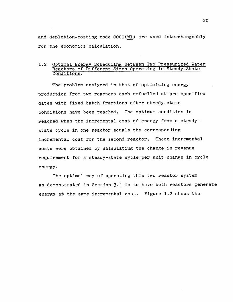
1.2 Optimal Energy Scheduling Between Two Pressurized WaterReactors of Different Sizes Operating in Steady-StateConditions.
The problem analyzed in that of optimizing energy
production from two reactors each refuelled at pre-specified
dates with fixed batch fractions after steady-state
conditions have been reached. The optimum condition is
reached when the incremental cost of energy from a steady-
state cycle in one reactor equals the corresponding
incremental cost for the second reactor. These incremental
costs were obtained by calculating the change in revenue
requirement for a steady-state cycle per unit change in cycle
energy.
The optimal way of operating this two reactor system
as demonstrated in Section 3.4 is to have both reactors generate
energy at the same incremental cost. Figure 1.2 shows the

21
F-.
*1i.-. I
FIG. 1.1INCREMENTALvs
COST*2. I
/,7 -
/9 .
A12
GO
.c* EYCVLL E/VE G Y /V
/0 /2./O GW$HE
.-.-,....
* . t * ,*. :.:
CYCLE ENERGYA 1065 MWe PWRB 430 MWe PWRIRRADIATION INTERVAL
1.375 YEAR
-.REFUELLING TIME0.125 YEAR
........ .
'4-I
1JJ
-- U
I

22.
-z.o Fics (jl
NUCLEAR. 5UB-5*1STE1-MjiNCREMErNTAL COST IS
TOTAL NUCLEAR..
I." NE RQ' PRODUCTIori
1-4
TO TAL NUC LE AR. ENERGY/ PRODOCT ION-z E." +EC1 10 lo;GW HE /C'lCLE
7 q 10 ' 1 -5 14 1- 1 '
-/ 4 i i i i

incremental cost versus the sum of energies generated by 23
the two reactors under the equal incremental cost rule.
The discontinuity point of the curve indicates that the
Zion reactor has reached its capacity limit, and from then on
any load increments goes to San Onofre. This curve can be
interpreted as the supply curve of the system. If the demand
curve is given, the intersection of the two curves give the
value of the equilibrium incremental cost, which can be
used in turn to calculate the optimal energy production for
each of the reactors. A detailed discussion of internal supply
and demand curve is presented in Widmers' thesis(W2).. Once
the optimal energy production of each reactor is know, the
corresponding reload enrichment can be found from Figure 1.3.
For this simple problem of steady-state operations,
fixed batch fractions and specified time schedule, the
problem of optimal energy scheduling and nuclear in-core
optimization can be solved easily by a set of graphs. For
non-steady state operations, however, the calculation of
revenue requirement and incremental cost is much more
complex. The following section indicates different ways of
calculating the objective function under non-steady state
conditions.
1.3 Calculation of Objective Function for Non-Steady StateOperations
Under non-steady state operating conditions, the physical
state of the reactor does not go through repetitive cycles.
Consequently, the end state of the reactor at the end of

24. I
R E LO A D
-4.2
R-3E NR %C%4E NT
CICLE E NER R
A 4Os lAe 'Pt)R
-4:1
LU
-c
.-3.6
-- -
e3
.-3o
2.6
a-
o,
R.CTR ENE RG 14h 41,3 4 wH e. / c vc La.
IT1 '~

25the planning horizon will not necessarily be the same as
the initial state at the beginning of the planning horizon.
Consequently, in order for the optimization to be effective,
an"end-effect'"correction must be incorporated into the
calculation of the objective function. The purpose of the
end-effect correction is to assign values to core inventories
which result in an objective function that varies only with
energy production within the planning horizon and not with
energy production in the neighboring time periods. If this
can be achieved, then optimization can be performed for
each individual planning horizon; the collection of such
optimal solutions would be the same as the optimal solution
for the entire life of the reactor obtained by a one-shot
calculation.
The object of the end-effect correction can be stated
mathematically as follows:
Let TC. be the revenue requirement for the entire life
of the reactor. Let TC be the revenue requirement for
planning horizon I which includes end-effect corrections.
The object of the end-effect correction is to equate
for F within
Er -r planning horizon I
c C (1.10)
This requirement can be called the condition of
"equalized incremental cost."

Two different methods have been investigated for 26
evaluating the end-effect correction. The Inventory Value
Method evaluates the worth of the nuclear core as the market
value of uranium and plutonium plus a fraction of fuel
fabrication, and post irradiation costs. The fraction of
fuel fabrication costs assigned to inventory value is (N-n)N
where N is the total number of cycles a batch of fuel
remains in the reactor and n is the number of cycles the
fuel has been in the reactor at the time the inventory
is to be valued. Similiarly, the accrual:of post irradiation
costs is treated by deducting n/N fraction of their total
from the inventory value.
The Unit Production Method evaluates the worth of the
nuclear core as the book value of the core based on straight
line depreciation according to energy production. In order
to obtain the salvage value of the core, the reactor is
operated past the end of the planning horizon under some
prescribed refuelling strategy until all the batches to
be evaluated have been discharged and their salvage value
determined.
Table 1.1 compares the incremental costs calculated
by the Inventory Value Method and the Unit Production
Method with the exact value. The Unit Production Method
gives more accurate incremental cost than the Inventory
Value Method. However, the Unit Production Method requires
more depletion calculations and is very sensitive to the

27
Table 1.1
Comparison of Exact Incremental Cost with Incremental Cost
Calculated by Two Approximate Methods
Incremental Cost for Cycle 1
- Mills/KWHe
Method Exact Approximate
InventoryValue
UnitProduction
6 E =1029GWHt
=2050GWHt
1.39 1.43 1.40
1.38 1.44 1.40

28prescribed refuelling strategy after the planning horizon.
Hence, the Inventory Value Kethod is recommended for use to
correct for end effects.
Having a method to correct for end-effects, and
consequently an acceptable method for calculating the
objective function, efficient ways of calculating approximate
incremental costs and reload enrichments for any required
set of energies are described in Section 1.4.
1.4 Calculation of Incremental Cost of Nuclear Energy Arcand Reload Enrichments for a Qiven Set of RequiredEnergies and For Fixed Reload Batch Fraction
Three methods to calculate the incremental cost of
nuclear energy Xrj will be described. The first, rigorous,
method is based on the definition of Arj; it is accurate
but time consuming. The second method is based on
inventory evaluation techniques; it takes less time, but
is less accurate. The third method is based on an approximate
linear relationship between reload enrichment and cycle
energy and again takes less time than the rigorous method
but is less accurate.
1.4.1 Rigorous Method
According to Equations (1.4) and (1.4a), the incremental
cost of nuclear energy is defined as the partial derivative
of the revenue requirement with respect to cycle energy,a T(C
rc DE r E rC c' (1.10a)

29which can be replaced by the forward difference
=-r(Eor Ear, EorA Ear ) ffr(For ~0 or o0rrc gg(E rE r,E r+AE,E+1.- T'E ,E,.E c11c 2 ' c 'c+l~ J.'2 '~c 'c+1"
AE
(1.11)If TC is known for two values of E c (e.g. in Equation
(1.11) for E r and E or+AE), while all the other Erc c ''c
are constant, Xrc can be evaluated quite easily. However,
to obtain the correct enrichments which permit Er to change
rwhile all other energies Ec, remain unchange is time-
consuming and expensive. The correct.enrichment for each
cycle must be found by trial. To determine all thel.rc
in an m-cycle problem requires about 3m(m+l) trials,2
using about three trials per cycle.
1.4.2 Inventory Value Method
In Section 1.3, the Inventory Value Method has been
shown to evaluate correctly the end effect and gives fairly
accurate values of incremental cost. If the Inventory Value
Method is applied at the end of the cycle for which
incremental cost calculation is desired, then incremental
cost of nuclear energy for that cycle can be obtained by
analyzing the change in the revenue requirement up to that
cycle as energy production changes in that cycle. Thus, all
later cycles need not be analyzed.

To calculate all the X in a planning horizon, onere
can proceed in the forward direction by first changing the
energy production of Cycle 1, applying the Inventory Value
Method and analyzing the change of revenue requirement up
to Cycle 1. This would be repeated for Cycle 2 and so on
until all the cycles have been analysed.
For an m-cycle problem, only 2m depletion calculations
are required to calculate all the incremental costs.
1.4.3 Linearization Method
This method makes use of the chain rule of partial
differentiation
r rBE r it E r i
r r r r r r =ac r ec c' c " BEc" Ece c c ' c" c
wlrWhen all and
Be rC
can be found by matrix
BE rc are known, then X rc
inversion. Evaluation of and
(1.12)
c
__E r
SC" is easier than X because reload enrichment E is anr rc c
explicit variable that can be controlled. The calculation of
each requires only (m-c+l) depletion calculations for an
c
m-cycle problem. Hence, to calculate all the 1rc, requires
only m(m+l) depletion calculations. The relationships2
between revenue requirement for indefinite planning horizon
TC, for finite planning horizon T, for the first cycle TO1 ,
various batches and cycles are shown schematically on Figure
30
r
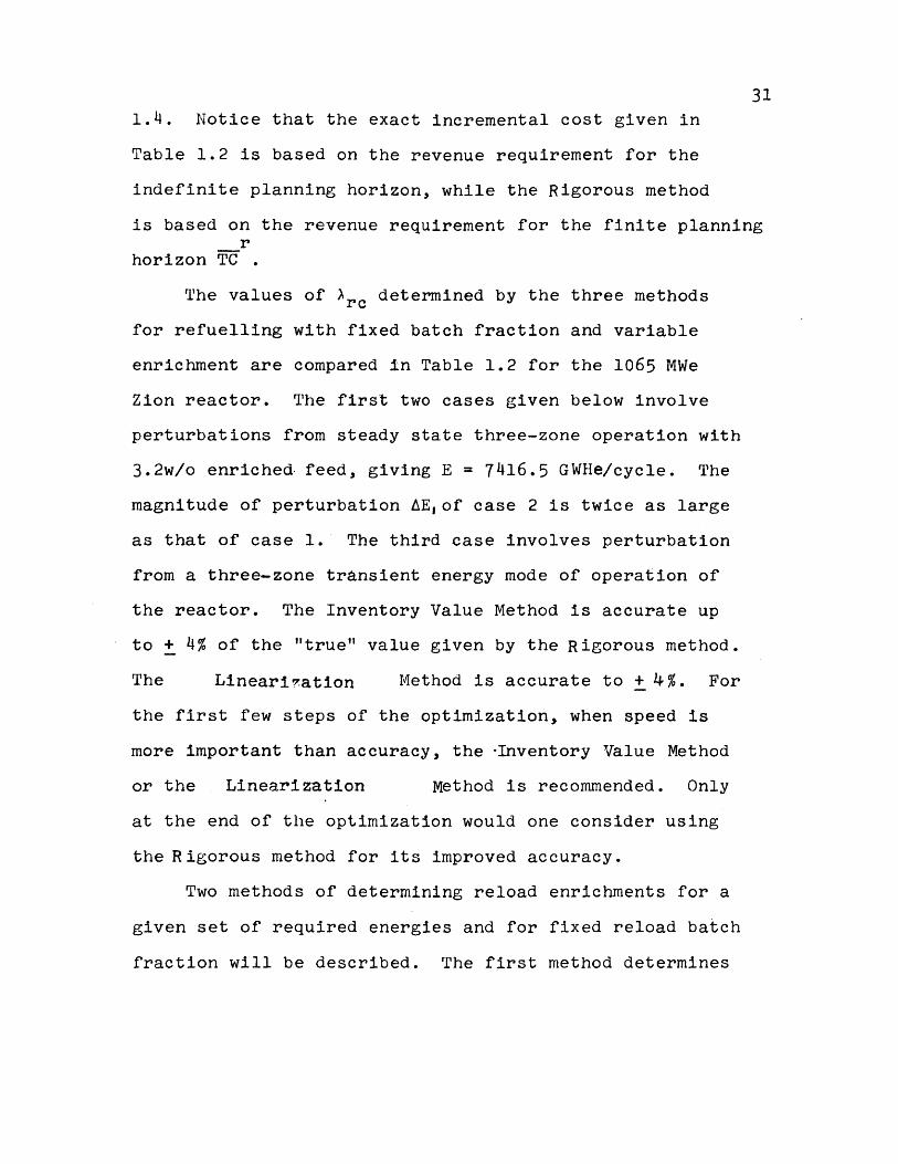
311.4. Notice that the exact incremental cost given in
Table 1.2 is based on the revenue requirement for the
indefinite planning horizon, while the Rigorous method
is based on the revenue requirement for the finite planning_r
horizon TC
The values of Arc determined by the three methods
for refuelling with fixed batch fraction and variable
enrichment are compared in Table 1.2 for the 1065 MWe
Zion reactor. The first two cases given below involve
perturbations from steady state three-zone operation with
3.2w/o enriched- feed, giving E = 7416.5 GWHe/cycle. The
magnitude of perturbation AE,of case 2 is twice as large
as that of case 1. The third case involves perturbation
from a three-zone transient energy mode of operation of
the reactor. The Inventory Value Method is accurate up
to + 4% of the "true" value given by the Rigorous method.
The Linearization Method is accurate to + 4%. For
the first few steps of the optimization, when speed is
more important than accuracy, the -Inventory Value Method
or the Linearization Method is recommended. Only
at the end of the optimization would one consider using
the Rigorous method for its improved accuracy.
Two methods of determining reload enrichments for a
given set of required energies and for fixed reload batch
fraction will be described. The first method determines

R~ NTio5H115 ETEE T-I VArciov kNrr.Q-~ Ni~
hKtD C*J-CLE~ N U WINER
.1
-II.PLANN INGHr 0OR 17 0l trb
-abo
REF L hT 10 W S Vi VPS a Er w F rc 14 TRE VARIOUS Ik r v F-N u . RSQU IRE t-AF- WS
'Tc

Table 1.2-
Incremental Cost of' lner'v 'alculhteel
by Three Methods
Incremental Cost byRigorous Method
1.42
1.40.
1.37
Incremental Cost byLinearization Method
1.37 -
1.37.
1.37
Incremental Cost byInventory Value Method
1.43
1.414
1.4:3
Case 1
Case 2
Case 3
LAJ

34reload enrichments by trial and error. For a given initial
state, two depletion calculations are carried out for one
cycle using two values of reload enrichments. The trial
enrichment for a given value of cycle energy is then
obtained by interpolating between the two values of
reload enrichments and the corresponding two values of
cycle energies. Three depletion calculations are usually
sufficient for any one cycle. Hence, for an m-cycle
problem, 3m trials are needed.
The second method determines reload enrichments by
an approximate linear relationship between cycle energy
and reload enrichment.
3Er r 0r,Er ~Eor + -E c (1.13)c c L r
3 ErSince all the coefficients c are made available
9Crby the Linearization Method in the calculation of
incremental cost, the determination of E, is a straight-
forward operation using matrix inversion. Table 1.3
shows values of reload enrichments calculated by the Trial
Method and Linearization Method for different sets of
cycle energies. Agreement between the two methods is
excellent. Hence, either method can be used.

Table 1.3Reload Enrichments Calculated by
(1) Trial Method and
(2) Linearization Method
Case 1
Cycle 1 2 3 4 5Energy Ei in 103GWHt 22.964 21.935 21.929 21.928 21.933Enrichment Ei (1) 3.359 3.054 3.174 3.196 3.133
(w/o) (2) 3.360 3.046 3.181 3.191 3.132
Case 2
Cycle 1 2 3 4 5Energy Ei in 103GWHt 23.985 21.919 21.906 21.937 21.970Enrichment j (1) 3.557 2.941 3.186 3.235 3.106
(w/o) (2) 3.557 2.928 3.197 3.225 3.108
Case 3
Cycle 1 2 3 4 5Energy Ei in 103GWHt 23.085 21.535 23.605 20.995 22.164Enrichment E (1) 3.359 2.975 3.545 2.833 3.286
(w/o) (2) 3.360 2.979 3.534 2.836 3.287
(jJ

36
1.5 Calculation of Incremental Cost and Nuclear In-CoreOptimization for Reactors Operating Under Steady-StateConditions
Starting from this section, batch fractions as well as
the reload enrichments are allowed to vary; only refuelling
times and energies are fixed. This section deals with
reactors operated under steady-state conditions. Hence,
there is only one reload enrichment variable and one batch
fraction variable for all the cycles. The problem of
nuclear in-core optimization under this special circumstance
is stated as follows:
minimize TC(Es ,E,f) for a given Es
with respect to e and f
subject to constraints F(s,f) = Es
B(c,f) < B*
the subscripts r, c are omitted because only one reactor
is considered and all cycles are the same under steady
state conditions. The revenue requirement for the first -
cycle is chosen to be the objective function.
For any combination of c and f, the reactor generates
a certain energy Es at a cost TC. By plotting TC vs Es
for all possible combinations of c and f, the optimal pair
can be found directly.
Figure 1.5 shows value of TC vs Es for different
combination of c and f for a Zion type 1065 MWe PWR refuelled
in a modified scatter manner. At cycle energies above 7000 Gwhe,
a batch fraction f = 0.33 results in lowest revenue requirement.
At cycle energies below 7000, a batch fraction of f = 0.25 is
preferable.

37fl7Tt~T
- R~&4 .G 1.5 _ _ -----
__VS&CYCL- EIEc Fc-K _ * . V/IWCu-s aATC,' 'mIciouMs.9
___ 0'
1*0 - r------ - 7 - -f
L _
--- - -- --- 2
. ....
4Lt -
H- 3 61- 8 9 /o _ __3
j77--7 I~~ - . .*..7 __ /0
// /0Aw
4
eyu.&9 e/GY
a

38.1
In Fig. 1.6, revenue requirement has been replotted
against batch fraction at constant cycle energy. In addition,
lines of constant average burnup BO are plotted. Only the
region to the right of a line of constant burnup is com-
patible with the burnup constraint (1.8). For example, at
the higher cycle energies of 10,650, 9,000 and 7,500 Gwhe,
with a burnup constraint of 30 MWD/kg, the optimum batch
fraction occurs at the burnup constraint rather than at the
lowest value of revenue requirement on the constant energy
line, at which
( af s 0(1.14))Es
When the optimum batch fraction is set by the burnup
constraint, in steady-state refueling a simple analytic
relation obtains between burnup B cycle energy Es, batch
fraction f and entire mass of uranium charged to the core W:
B-W-f = Es (1.15)
Hence, the smallest batch fraction that satisfies the burnup
constraint B* is given by f = Es/(B*W). (1.16)
Figure 1.7 shows the optimal batch fraction as a function
of cycle energy for different burnup constraints. For high values
of maximum allowable burnup and low cycle energies, the optimal
batch fraction is determined by the economic optimization con-
dition Eq.(l.14), whereas at higher cycle energies or lower
allowable burnup it is given by Eq.(1.16).

38.2
In Figure 1.8 revenue requirement TC is plotted against
reload enrichment, with lines of constant batch fraction f or
cycle energy E or average burnup BO. The optimal values of
reload enrichment and batch fraction to produce specified
energy can be read off directly for a specified burnup
constraint B4 or minimum revenue requirement.

39
P=C., 1.6 REVsAU RE.REM VSBiATCi =2AC-ON /F ~Ok7 Pitf=P.ERET
L 4-VL& CP V'= R6-V
e. L ~i RRAD1/rnO1V PERIODC A P ACiTY 1=ACro'
aL~ / -RRADI AThc/V .;1VrLRVAL
- RFU~E4.IN'6, Sif}7DCWNI ~O./Qw V'iAR/
C 0. 2 0,3 0.4 0. 0A TCH FR ACT I ON

410
FIG. 1.7 OPAIAL BATC#i (~RACThON V5C YCL RG r-o/ VACicLus ,U/?/UP
* .I li l I I
C100&
- s
D R iAI T~1CN \/IATE A LREG,/=u FL iA/VG TIME 9 C.4
N-7 o e
~O.- /2
1I.

41
FIGURE 1.8
REVENUE REQUIREMElWT VS RELOAD
ENiRICIHElT FOR VARIOUS LEVELS OF ElERGY
-:20
1*3-75 YRN. ll?RAD, /Wi"RAL

42
The calculation of incremental cost of energy for the
case of variable reload enrichment and batch fraction
deserves special attention. According to Equations (1.4)
and (1.4a) X is given as
_TC(EsS*,f*) where S* and f*
are optimal
solution for Es
which can be expanded into the following finite difference
relationship
TC(Es+AE, et, ft) - TC(Ess*,f*) (1.17)AE
where c and ft are the optimal solution for Es + AE. When
there are no constraints on the enrichment and batch fraction, c
and f are those values at which the revenue requirement is a
minimum for a particular energy, i.e. the minima of the constant
energy lines in Fig. 1.6. When the maximum burnup B* places
lower a limit on the batch fraction with which a particular
energy may be produced, as in the case at a value of B* of
30 MWD/kg at energies above 5,000 Gwhe, the values of revenue
requirement used in Eq. 1.17 are those on the constant burnup
line of Fig. 1.6. Fig. 1.9 shows values of incremental
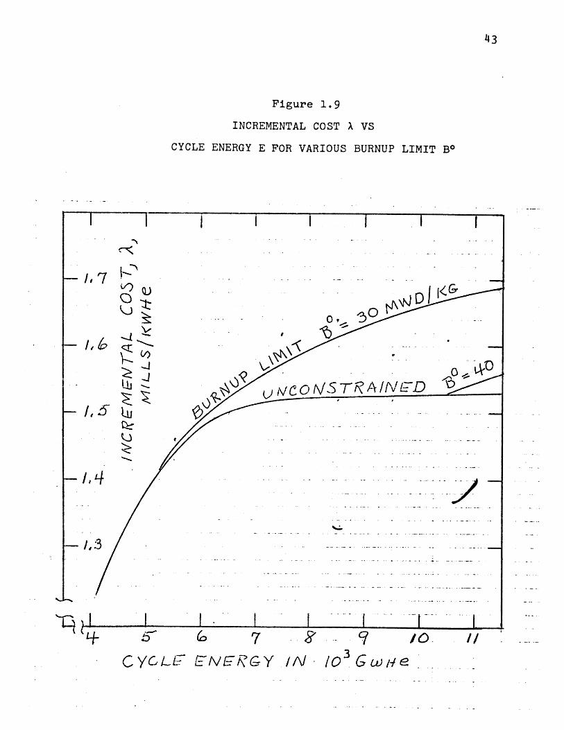
43
Figure 1.9
INCREMENTAL COST X VS
CYCLE ENERGY E FOR VARIOUS BURNUP LIMIT B*
-- 7 [Y. ||
-CCIG~CNER)C, // -/03 Gw.

44
.1.1
lKVZHNl4TL CO~ST 7 .
CJ CLE E NERQI E
TO~R VAROV SBURNILP W RIT ISO
0
0
CAPActTJ~ ,FptCTOR..
O.ij~~flowl-0
0.6-AS6 0 *-flqRT OAq3IOI I
'C JCLE
60
ENERG~'/
9IN 10G h~e./cSCLE.
to01I I
IRRADIAMOc* *aTEXAJ AL
RETUELIN't TIMIE
ft
1~~-
-1.1
ILl.

44 -45cost of energy versus cycle energy for different values
of burnup limits. Initially, incremental cost increases
rapidly with respect to cycle energy but gradually levels
off. As the burnup limit decreases, incremental cost
increases.
For this special case of steady state operation, the
problem of nuclear in-core optimization and the calculation
of incremental cost involves a relatively small number of
variables and can be handled effectively by graphs. For
non-steady state operations, however, there are so many
variables that complicated optimization techniques such as
piece-wise linear approximation, or polynomial approximation,
coupled with total exhaustive search, is required to solve
this problem. Sections 1.7 and 1.8 summarize the methods and
results of the two approaches. But before that, tests
are required to show that the objective function calculated
by the Inventory Value Method is suitable for this pur-
pose.
1.6 Test of the Objective Function for the Variable Batch
Fraction, Non-Steady State Case
As mentioned earlier in Section 1.3, a method for
calculating the objective function for a finite planning
horizon is deemed adequate for the puroose of scheduling
energy if it gives the same value of incremental cost of
energy as an exact calculation in which the entire life span
of the reactor is considered.

..- 46ie aTC = for all j withinD BE planning horizon I
(1.18)
However, for the problem of nuclear in-core optimization,
the following additional equations for the partial derivatives
are involved:
-TI for all c withinc c planning horizon I
(1.19)
If these equalities are maintained throughout the
optimization, as demonstrated in Section 7.3, the collection
of optimal solutions for each of the finite planning horizons
would be the same as the overall optimization performed
on the entire life span of the reactor. Table 1.4 shows
values of the ATC./Ae and ATC /Ae versus enrichment changes
1c and values of ATC /Af and ATC 1/Af versus batch
fraction changes Af for Cycle 1. It can be seen that the1
finite planning horizon objective function can be seen to
give accurate first order derivatives for Cycle 1. Since
nuclear in-core optimization would in all probability be
updated on an annual basis, only the first cycle results
would actually be utilized. Hence, the main emphasis on
accuracy would be placed on the first cycle derivatives.
Having demonstrated that the finite planning horizon

Table 1.4
Effect of Variation of Enrichment and Batch Fraction on Revenue Requirement
TcRevenue Requirement for the Indefinite Planning Horizon
T~C Revenue Requirement for the Finite Planning Horizon
EnrichmentChanges
(w/o)& E ,
-1.200-0.434+0.480+1.200
Batch FractionChanges
-0.8-0.4+0.4
Revenue RequirementChanges 610 $
-4.570-1.6648+1.8893+4.6642
-4.5804-1.6746+1.8791+4.6542
Revenue RequirementChanges 6
10 $
-2.3494-1.1717+0.7716
-2.3623-1.1822+0.7658
10 6 $/(w/o)
3.81003.83603.93613.8868
3.81693.85863.91483.8785
TCI/af T aa/&f1io6
2.93672.92931.9290
2.95282.95541.9146
Error
+0.2+0.6-0.5-0.2
Error
+0.5+0.9-0.7

48objective function is suitable for nuclear in-core
optimization, Section 1.7 and 1.8 proceed to describe
the piece-wise linear approximation approach and the
polynomial approximation approach of solving the
optimization.
1.7 The Method of Piece-Wise Linear Approximation for theProblem of Nuclear In-Core Optimization
In the Method of Piece-Wise Linear Approximation, the
objective function and the constraints are linearized
about an initial feasible solution. For example
TC= T(I",) + a c C- ) + L Rf -f0) (1.20)
where
a c C(Z,* 3T 97*C C
The expansion coefficients ac and S are determined
by a number of perturbation cases in which the decision
variables are varied one at a time. For example
C , * .A . (1 .21)
Linear programming can be applied to the set of
linearized objective function and constraints. Limiting
the changes in Af/f by + 1% each time, a new solution
can be calculated in the steepest descent direction. The
process of linearization and optimization can be repeated
on this new solution in an iterative fashion.

49Unfortunately, practical mesh spacing setup of the
present CELL-CORE depletion code only allows discrete
changes of Af/f by 12%. Hence, the linear model must
be modified to accommodate changes by large step sizes.
The final form of the equations used is slightly
more complicated than the illustrative Equation (1.20).
Instead of having a single expansion coefficient for each
variable, there are two expansion coefficients, one for
positive and one for negative variation of the batch
fraction variables. The set of piece-wise linear equations
are solved by total exhaustive search. The objective
function is calculated for all feasible neighboring points
around the initial solution. The neighboring point with
the lowest objective function is chosen to be the new
solution on which linearization and optimization are to be
repeated.
As an example of the application of this method,
consider the following sample case A. The reactor under
analysis is the Zion type 1065 MWe PWR with initial condition
equivalent to the 3.2 w/o three-zone modified scatter
refuelled steady-state condition. The planning horizon
consists of five cycles. Energy requirement for each of
the five cycles is 22750 GWHt, the same value as produced
in the steady-state condition. The maximum allowable
average discharge burnup is 60 MWD/kg. The Method of
Piece-Wise Linear Approximation is applied to solve for the
optimal reload enrichments and batch fractions for the five
cycles.

Table 1.5 shows the batch fractions, reload enrich-
ments, cycle energies and revenue requirement for the various
iterations. The revenue requirement is calculated based
on economic parameters similiar to that of TVA, with no
income tax obligations. The revenue requirement. corrected
for target energy decreases in successive iterations. The
final solution results in net savings of $1.6 million
dollars when compared to the initial solution. However, when
the same 'case is repeated using the economics parameters
characteristic of an investor-owned utility which pays
income taxes, the Method of Piece-Wise Linear Approximation
fails to converge. This is due to the fact that the
original initial condition 3.2 w/o three-zone modified
scatter refuelling is so close to the optimal solution that
piece-wise linear approximation based on step size
of 12% is too large for the purpose.
This method of Piece-Wise Linear Approximation is
applicable to cases where the objective function has a
wide variation over the range of the decision variables,
and where the optimal solution is ultimately limited by
one or more of the constraints. However, if the objective
function is rather flat and the constraints are not active,
the Method of Piece-Wise Linear Approximation cannot pin-
point the optimal solution precisely, and a more
sophisticated technique like polynomial approximation
is needed.

Table 1.5
Reload Enrichments, Batch Fractions, Cycle Energies and Revenue Requirements for
Various Number of Iterations Usirg the Method of Piece-Wise Linear Approximation
Cycle
1 2 3 4 5
c(w/o)fE(GW-t)
Revenue Requirement
For Actual Energy
Piece-wise CELL-Linear COCOAppro-ximation
Corrected forTarget Energy
Piece-wise CELL-Linear COCOAppro-ximation
TargetEnergy
IterationNumber
0 EfE
1 EfE
2 efE
3 EfE
22750. 22750. 22750. 22750. 22750. 106
3.20.33322750.
3.770.29322257.
5.030.25322697.
3.950.29322986.
3.20.33322750.
3.370.29322725.
3.030.25322534.
4.250.25323133,
3.20.33322750.
3.450.29322616.4.270.25322844.4.640.21322325.
3.20.33322750.
3.560.29323076.2.960.25322430.
4.310.21323894.
3.20.33322750.
3.420.29322769.
4.570.25322646.
3.610.21321253.
72.1119 72.1119
71.3358 71.1517
70.3096 70.5269
70.0805 70.4763
72.1119 72.1119
71.4971 71.3131
70.4969 70.7141
70.2485 70.6443
\H

521.8 The Mathod of Polynomial Approximation for the
Problem of Nuclear In-Core Optimization .
In the Method of Polynomial Approximation, the
objective function and the constraints are approximated by
a sum of polynomials in cycle energies and batch fractions.
For example
7- a i E m. fm nc -= n3clmn c c c-1
(1.22)
B = eklmn c c-1 cc-1c k=-i 1=-1 m=-3 n=-3 (1.23)
The expansion coefficients clmn, cklmn are multiple
regression coefficients based on analysis of a large number
of sample cases. For cases considered here, the polynomial
can be fitted with an accuracy of + 0.1% of TC and + 5% of
B. using polynomials up to the third order.
The objective function and the constraints in polynomial
form can be optimized analytically. Since the energy
requirement is implicitly included in Equation (1.22) the
only independent variable is the batch fraction fc-
The objective function TO and the discharge burnup Be
are calculated for all possible values of f. The TC with
the lowest cost satisfying a certain burnup limit B* is
chosen as the optimal solution.
The following two sample -cases are analyzed by this
method. Sample case A is identical to the problem

considered in the previous Section 1.7 by the Method of 53
Piece-Wise Linear Approximation, with economic parameters
that included income tax. Sample case B differs from
sample -case A in that the cycle energy requirements are
different for different cycles.
Table 1.6 shows values of reload enrichments, batch
fractions cycle energies and revenue requirement for
sample case A for the seven cases having the lowest
costs. AAO is the base line case, where the batch fractions
and reload enrichments are held at the original steady
state values. Net savings in the order of 0.3 million
dollars are achieved in case ABl when compared to steady-
state operation AAO through this optimization. Table 1.7
shows values of discharge burnup estimated by the polynomial
approximation as compared to the actual values given by
CELL-CORE. The results agree within +5%.
Sample case B differs from sample case A in the
cycle energy requirement. Cycle energy requirements vary
for Sample problem B and are:
E1=25450. GWHt, E2=30440. GWHt, E3=21850. GWHt,
E4=19340. GWHt, E5=20880. GWHt
Table 1.8 shows values of reload enrichments, batch
fractions, cycle energies and revenue requirements for the
five solutions having the lowest costs. BAO is the base
line case, where the batch fractions are held constant at

Table 1.6 B% 50MWD/KgReload Enrichments, Batch Fractions, Cycle Energies and Revenue Requirements for theVarious Lowest Cost Cases Using the Method of Polynomial Approximation Sample Case A
TargetCase Energy
22750. 22750. 22750. 22750.22750.
3.20.33322750.
30880.29322690.
3.880.29322690.
3.880.29322690.
3.880.29322690.
3.880.29322690.
3.880.29322690.
3.880.29322690.
Revenue RequirementFor Actual Energy Corrected for Target
Poly- CELL-nomial CocoAppro-ximation 6
Energy_Poly- CELL-nomial CoCo
ximation
(Difference)87.30 87.24 87.30 87.24
(+0.06)
86.43 86.34
87.20 87.33
87.09 87.13
86.26 86.37
86.82 86.89
86.94 87.00
87.23 87.14
86.99(+0.09)
87.01(-0.13)
87.02(-0.04)
87002(-0.11)
87.03(-0.07)
87.04(-0.06)
87.04(+0.09)
86.90
87.14
87.06
87.13
87.10
87.10
96.95
Uq
Cycle
fE (GWHt)
2 4 5
NumberAAO
AB1
AB2
EfE
9fE
e
E
AB3 EfE
3.20.33322750.
2.400*29320500.
3.450.29323070.
2.940.33323030.
2.400.33319730.2.660.29322300.
3.450.29322830.
3.610.25323250.
3.20.33322750.a
4.270.25323000.
4.270.25323000.
30330.29322840.
4.270.25323000.
3.290.29322700.
3.290.29322700.
4.270.25323000.
3.20.33322750.
3.420.25322480.
2.760.29322510.
3.450,29322560.
2.770.29322510.
3.450.29322400,
3.450.29322460.
3.420.25322480.
3.20.33322750.
3.950.25323100.
3.770.29323130.
30540.29322920.
3.740.29322980.
4.500.25323000,
3.540.29322880.
3.950.25323090.
AB4
AB5
AB6
AB7
17fE
EfE
efE
EfE

B" =50MWD/Kg
Average Discharge Burnup for the Sublot Experiencing the Highest Exposure for Sample
Case A Calculated by (1) Polynomial Approximation Based on Regression Equations
(2) CELL-CORE Depletion Calculation
BatchNumber
CaseNumber
-2 -1 0
Method
AAO (1)(2)
AB1 (1)(2)
AB2 (1)(2)
AB3 (1)(2)
AB4 (1)(2)
AB5 (1)(2)
AB6 (1)(2)
AB? (1)(2)
31.531.538.638.9
38.638.938.638.9
38.638.9
38.6386938.6386938.638.9
31.531.538.6386438.638.4
38.638.6
38.6386438.638.6
38.638.6
38.638.4
31.5316538.638.1
38.638.538.638.8
38.638.538.6386838.638.838.638.1
. I 2
-MWD/Ks31.531.5446244.444.245.244624469446245.2
44.244.5446244.944624464
3
31.531.547.446.9
47.447.5
3964396447.447.3
39.438.4
396438.7
47.44760
4
31.5 31.5
40.4 44.4
34.7
4069
34.7
4069
40.9
4064
43.2
4162
4362
49.6
41.2
44.4
_5
31.5
31.8
36.4
3661
31.9
34.3
40.6
3862
Un
Table 17

Reload Enrichments, BatchTable 1.8 B0 MO!VWD/Kg
Fractions, Cycle Energies and Revenue Requirements for theVarious Lowest Cost Cases Using the Method of Polynomial Approximation. Sample Case B
Li.C (w/o) ifE(GW~it)
Target 25450.Energy
3.730.33325510.3.740.33325510.
4.550.293-25340.
3.740.33325510.
4.550.29325340.
4.550.29325340.
CaseNumber
BAO cfE
BB1 efE
BB2 cfE
BB3 CfE
BB4 efE
BB5 EfE
30440. 21850. 19340. 20880.
4.360.33330470.4.360.33330470.
3.790.33330310.
2.400.33322170.
2.700.29321270.
2.910.29321790.
4.36 2.700.333 0.29330470.'21270.
3.79 2.910.333 0.29330310. 21790.3.79 3.720.333 0.25330310. 21790.
2.760.33320280.
3.880.25319180.3.870.25319480.
3.100.29319260.
3.090.29319320.2.930.25319130.
3.450.33317220.
2.270.29317930.2.610.29320020.
2.370.33317480.2.710.33319930.2.930.29320110-
Revenue RequirementPor Actual Energy Corrected for Target
EnergyPoly- CELL- Poly- CELL-nomial COCO nomial COCOAppro-ximation 6
10 $-
89.36
88.66
89.35
88.61
89.32
89.31
Appro-ximption
(Difference)
89.37 89.92(-0.01)
88,71
89.38
88.67
89.38
89.27
89.67(-0.05)
89.67(-0*04)
89.71(-0.05)
89.71(-0.05)
89.72(+0.04)
89.93
89.72
89.71
89.76
89.76
89.68
,
-Cycle-2
57the 0.33 level and serves as a standard for comparing other
cases. Net savings of 0.25 million dollars achieved by
Case BB5 are realized when compared to base case BAO.
Table 1.9 shows values of discharge burnup estimated by
the polynomial approximation as compared to the actual
values given by CELL-CORE. The same accuracy as in sample
case A is achieved.
The results of regression analysis and the optimization
procedure indicate that the objective function is rather
insensitive to batch fraction changes, if the same cycle
energies are produced. In the two sample casles given
above, using the base line cases instead of the optimal
cases only incurred additional cost of 0.3 million dollars,
which is amere. 0.4% of the total revenue requirement. If
the base line cases give better engineering margins in terms
of discharge burnup, power peaking and shut down reactivity,
they should be used instead. The final choice should be
based on engineering margins rather than on economics.
Finally, a method of calculating incremental cost of
energy under the variable batch fraction, non-steady
state operating conditions are given. The method is based
on taking finite differences on the regression equation
involving TC. The incremental cost of energy for cycle c
is given by
TU(E ,E,.+AE,..t) - TC(E i ,..20)c
AE h (1I.2Z4 )

Average Discharge Burnup for the Sublot Experiencing the Highest Exposure for Sample
Case B Calculated by (1) Polynomial Approximation Based on Regression Equations
(2) CELL-CORE Depletion CalculationBatchNumber
-2 -1 0 1 2 3 4
Case MtoNumber Method
BAO (1)(2)
BB1 (1)(2)
BB2 (1)(2)
BB3 (1)(2)
BB4 (1)(2)
BB5 (1)(2)
31.531.531.531.538.639.2
31.531.538.639.2
38.639.2
31.531.831.531.838.639.831.531.838.639.838.639.8
31.532.8
38.639.338.639.738.639.338.639.738.639.4
-MWD/Kg--37.2 43.937.9 42.2
43.044.949.752.243.045.649.752.7
49.751.7
48.249.4
43.544.048.250.2
43.544.743.544.1
31.928.5
34.4
36.2
34.4
36.2
42.9 36.3
Notice that the B =50MWD/Kg 1imit only applies to the estimated burnup valuescalculated by the polynomial regression equation. -The fact that actual burnup valuessometimes exceed 50MWD/Kg indicates that the estimated burhup values are only approximate.
UnCO
35.032.944.3
44.1
37.8
37.6
41.441.9
30.9
33.7
31.7
34.6
36.4
Table 1. 9 B*0=50MWD/Kg

59
where ft and f* are the optimal batch fractions for
the gs + AEc and the is case respectively.
that is TC (9s + AECft ) = minimum TC(Is + AEc '
with respect to f
and TC(Es ,f) = minimum T(9sf)
with respect to f
Tables 1.10 and 1.11 show values of f*, ft , TC and AC
for various values of Ec and for various burnup limits
based on the optimal solution of sample case A.
Tables 1.12 and 1.13 show the same quantities for sample
case B. It can be seen that the incremental cost in
a cycle varies irregularly with cycle energy. This is
due to the fact that different sets of f are needed to
satisfy the burnup constraints for different cycle energy
requirements. The variation of TC with respect to these
different sets of f is not continuous.
1.9 Conclusions
The following conclusions are obtained from this
thesis research.
(1) The Inventory Value Method for evaluating worth
of nuclear fuel inventories t6 be used in

60
Table 1.10
Calculation of Incremental Cost of Energy
Using Regression Equations. Sample Case A
Burnup Limit B= 45MWD/Kg
Batch Fraction for Cycle
1 2 3
0.293 0.293 0.293
RevenueRequirement
-- 106$4 5
0.293 0.293 87.01872
Incre-mentalCostin Mills/
KWHe
Positive Energy Change&E=1OOOGWHtin Cycle
1 0.333 0.293 0.293
2 0.293 0.293 0.293
3 0.293 0.293 0.293
4 0.293 0.293 0.293
5 0.293 0.293 0.293
Negative Energy ChangeAE=-1000GWHtin Cycle
1 0.293 0.293 0.293
2 0.293 0.253 -0.253
3 0.293 0.293 0.293
4 0.293 0.293 0.293
5 0.293 0.293 0.293
0.293 0.333 87.5284
0.293 0.333 87.4265
0.293 0.333 87.3890
0.293 0.333 87.3170
0.293 0.333 87.2957
0.293 0.333 86.5642
0.253 0.293 86.5848
0.293 0.333 86.6605
0.293 0.333 86.7226
0.293 0.333 86.7443
BaseCase
AA1
1.56
1.22
1.15
0.91
0.845
1.395
1.33
1.095
0.905
0.84

Table 1.11
Calculation of Incremental Cost of Energy
Using Regression Equations. Sample Case A
Burnup Limit B =50MWD/Kg
Batch Fraction for Cycle RevenueRequire-
1 2 3 4 5 ment
BaseCase 0.293 0.253 0.253AB1
Positive Energy ChangehE=1000GWHtin Cycle
1 0.293 0.253 0.253
2 0.293 0.293 0.293
3 0.293 0.253 0.293
4 0.293 0.253 0.253
5 0.293 0.253 0.253
Negative Energy ChangeAE=-1000GWHtin Cycle
1 0.293 0.253 0.253
2 0.293 0.253 0.253
3 0.293 0.253 0.'253
4 0.293 0.253 0.253
5 0.293 0.253 0.253
0.253 0.293
0.253 0.293
0.293 0.333
0.293 0.293
0.253 0.293
0.253 0.293
0.253 0.293
0.253 0.293
0.253 0.293
0.253 0.293
0.253 0.293
-106$-
86.9890
87.4642
87.4265
87.3848
87.3047
87.2748
86.5345
86.5848
86.5860
86.6761
86.7064
Incre-mentalCost
in Mills/KWHe
1.46
1.335
1.21
0.965
0.875
1.395
1.24
1.24
0.955
0.865

62
Table 1.12
Calculation of Incremental Cost of Energy
Using Regression Equations. Sample ease B
Burnup Limit B=45MWD/Kg
Batch Fraction for e
1 2 3 4 5
BaseCase 0.333 0.373 0.293 0.253 0.293BA1
RevenueRequire-ment
106$---
89,8251
Incre-mentalCost
-Mills/KWHe-
Positive Energy ChangeA E=1000GWHtin Cycle
1 0.333 0.373 0.293 0.253 0.293
2 0.333 0.373 0.293 0.253 0.293
3 0.333 0.373 0.293 0.253 0.293
4 0.333 0.373 0.293 0.293 0.333
5 0.333 0.373 0.293 0.253 0.293
Negative Energy ChangeAE=-1OOOGWHtin Cycle
1 0.333 0.373 0.293 0.253 0.293
2 0.333 0.373 0.293 0.253 0.293
3 0.333 0.373 0.293 0.253 0.293
4 0.333 0.373 0.293 0.253 0.293
5 0.333 0.373 0.293 0.253 0.293 89.5484
90.2916
90.2424
90.1845
90.1255
90.1049
1.435
1.28
1.10
0.91
0.915
89.3766
89.4070
89.4773
89.5224
1.375
1.28
1.07
0.925
0.85

63
Table 1.13
Calculation of Incremental Cost of Energy
Using Regression Equations. Sample Case B
Burnup Limit B =50MWD/Kg
Batch Fraction for Cycle
1 2 3 4
0.333 0.333 0.293 0.253 0.293
RevenueRequire-ment
-106
89.6715
Incre-mentalCost
Mills/KWHe
Positive Energy ChangebE=100OGWHtin Cycle
1 0.333 0.333 0.293 0.253 0.293
2 0.293 0.333 0.293 0.253 0.293
3 0.333 0.333 0.293 0.253 0.293
4 0.333 0.333 0.293 0.253 0.293
5 0.333 0.333 0.293 0.253 0.293
Negative Energy ChangeAE=-1000GWHtin Cycle
1 0.293 0.333 0.293 0.253 0.293
2 0.293 0.293 0.253 0.253 0.293
3 0.333 0.333 0.253 0.253 0.293
4 0.333 0.333 0.293 0.253 0.293
5 0.333 0.333 0.293 0.253 0.293 89.3947
BaseCaseBBI
90.1380
90.0775
90.0309
89.9772
89.9513
1.435
1.25
1.10
0.93
0.86
89.1628
89.1515
89.3229
89.3687
1.56
1.60
1.07
0.925
0.845

calculating finite planning horizon revenue
requirement is adequate for the purpose of
scheduling energy and nuclear in-core
optimization.
(2) Three methods are proposed for calculating
incremental cost of energy for the fixed batch
fraction case. The Linearization Method
and the Inventory Value method for calculating
incremental cost of energy are both suitable
for the initial stages of optimal energy
scheduling. The Rigorous Method is very time-
consuming and expensive and should be used only
in the final stages of optimal energy scheduling.
(3) For the problem of nuclear in-core optimization
under steady state conditions with variable
batch fractions and reload enrichments, the
optimal solution is practically always on the
boundary of the burnup constraints. Hence,
there are strong incentives to increase the
burnup limits.
(4) For the problem of nuclear in-core optimization
under non-steady state conditions, the Method
of Piece-Wise Linear Approximation is applicable
for the cases where there are large variations
of objective function near the optimal solution.
It is not applicable for economic situations where

65
there is a broad region of optimality.
(5) The Method of Polynomial Approximation gives
accurate values of the optimal solutions, even
though the objective function is very flat
near the optimum.
(6) Since the objective function is insensitive to
large variations in batch fractions, selection of
the optimal solution can be based primarily on
other considerations, such as engineering margins.
1. 10 Recommendations
The depletion code CELL-CORE should be modified in
order that the batch fraction can be varied continuously.
This modification would enable the efficient usage of the
Method of Linear Approximation instead of Piece-Wise Linear
Approximation or Polynomial Approximation. Once the optimal
batch fraction in the continuum is located, the realistic
batch fraction to be used in refuelling would be given by
the number of integral fuel assemblies which is closest
to the continuum optimal solution.
Finally, the algorithm of optimal energy schedule
should be modified so that the polynomial equations from
regression analysis could be used directly, instead of the
present indirect usage which require intermediate calculations
of incremental cost. It is recommended that a quadratic
programming algorithm, or an even higher order programming

66algorithm should be used in the optimal energy scheduling
procedures, so that the higher order derivatives can be
used directly.

CHAPTER 2 67
INTRODUCTION
2.1 Motivations for Mid-Range Utility Planning
Until recently, procedures for scheduling energy
production from different nuclear power plants in an electric
utility system have consisted of a relatively simple set of
rules. All the nuclear power plants were to be operated
base-loaded whenever they were available. They were to be
refuelled annually, either in the spring or in the fall when
the system demand is at its lowest level. From an economics
stand point, the foregoing rules can be justified because
nuclear energy, being cheaper than conventional fossil energy,
should be used whenever possible to displace the latter.
Annual refuelling is desirable from an operational standpoint.
For electric utilities having only a small number of
nuclear units, this is a practical and economical way to
operate nuclear power units. However, recently the number
of nuclear power units in some large utilities, such as
Commonwealth Edison and Tennesse Valley Authority, have
increased to such a level that the foregoing rules are not
sufficient for the following reasons. The combined nuclear
generating capacity is so large that all of them cannot
be operated base-loaded in periods of low system demand.
Another reason is that there are so many nuclear power units
that all of them cannot be refuelled annually during the
spring and fall without creating some operating and reliabil-
ity difficulties. For example, refuelling two or more reactors

68at the same site simultaneously or successively might create
excessive strain on the grid in the region to which these
reactors belong and might also overload station refuelling and
maintenance personel operations. Consequently, the following
requirements in refuelling are being considered (Q)
(i) From the standpoint of area security, no
more than one reactor should be down for refuelling
for any region at any given time.
(ii) From the standpoint of efficient refuelling
operations, reactors should not be refuelled
simultaneously or successively at a given site.
(111) From the stand point of satisfying the system
demand, all the nuclear power units should be
available in the peak demand periods. Hence,
nuclear power units cannot be scheduled for
refuelling in the summer if there is a severe
summer peak.
Under these requirements annual refuelling can no longer
be maintained for all nuclear reactors at all times. In this
situation reactors cannot be base-loaded all the time and
refuelled annually.
New scheduling methods must be developed that will
handle this situation. These methods should provide an
optimal operating schedule for energy production for all
the generating units (fossil, hydro and nuclear) in agiven
electric utility spanning a planning horizon of more than
five years. Besides specifying energy production for every
unit, the schedule should also specify refuelling and

69maintenance dates for each unit and other refuelling
details for nuclear reactors,such as reload enrichments
and batch fractions. This overall problem of scheduling
is called Mid-Range Utility Planning.
2.2 Formulation of the Overall Optimization Problem forMid-Range Utility Planning
The overall optimization problem for Mid-Range Utility
Planning can be formulated as follows; given a load forecast
for a given electric utility over the span of the planning
horizon, given the composition of the electric utility in
terms of the capacity, type and locations of each generating
unit, find the optimal schedule of operation which consists
of refuelling and maintenance dates, energy production in
each time period for every unit, and (for all nuclear
reactors) the reload enrichments and batch fractions for
each cycle in the planning horizon.
The objective function for this problem is the revenue
requirement directly related to energy production in the
planning horizon. This is the capital which if received as
revenue by the company at time zero which, invested in the
company at the effective rate of return x, would enable the
company to pay all fossil and nuclear fuel expenses startup
and shutdown costs, other variable operating costs, and all
related taxes, pay bond holders and stock holders their
required rate of return on outstanding investments on
nuclear fuels, and retire all fuel investments at the end
of the time horizon. The fuel revenue requirement for the

70electric utility is the sum of all these revenue require-ments for each generating units:
R
r (2.1)
where Tr is the total revenue requirement for thesystem
TCT is the revenue requirement for unit r
R: total number of generating units in the system.
The decision variables are
(i) time for maintenance and refuelling for each unit
(ii) energy production of each unit for each periodof time in the planning horizon
(iii) for the nuclear generating units, the reloadenrichments and batch fractions for each cycle.
In general, there are other parameters specific to the
nuclear generating units; such as refuelling pattern,
configuration of burnable poison rods, multi-enrichment
batches etc. For the sake of simplicity, these parameters
are not included in the decision variables.
The constraints for this problem are:
(i) the sum of energy production from all of the
generating units must be equal to the total
system demand in each period of time.
(ii) Rate of energy production for each unit cannot
exceed its rated capacity.
(iii) Each nuclear reactor should operate within its
physics and engineering constraints, for example,
burnup limits, power peaking factors and reactor
shut down margins.

(iv) Other system operating restrictions such as 71
area security, spinning reserve requirements
limitations on startup and shutdown frequency
etc. must be met.
(v) Refuelling schedules must meet the restrictions
as specified in Section 2.1. For a complete
listings of the cons'traints refer to Widmer (W2)
or Deaton (DJ). For the purpose of this thesis
research, only a few of these constraints are
explicitly considered, and they will be stated
clearly in each chapter. Some of the physics
and engineering constraints for nuclear reactors
are investigated in greater depth in Kearney's (&)
and Rieck's (B) thesis research.
2.3 Decomposition of the Overall Problem into VariousSub-Problems
The overall optimization problem of Mid-Range planning
can be decomposed into three sub-problems. The first sub-
problem deals with the decision variable of maintenance and
refuelling times. A computer code has been developed by
John Bukovski (CZy) that generates a number of refuelling
and maintenance schedules compatible with specified
constraints. For each refuelling and maintenance schedule,
the second sub-problem involves finding the energy pro-
ductions, reload enrichments and batch fractions for the
generating unit which lead to lowest cost. This is repeated
for each time schedule, and the schedule with the lowest

cost is chosen to be the optimal solution. The third 72
sub-problem involves separating the problem of optimal
energy schedule from nuclear in-core optimization and then
the energy variables from the enrichment and batch fraction
variables. In essence, this technique of decomposition
separates the time dependence from the other decision
variables. Hence, the overall optimization problem of mid-
range planning reduces to solving for the optimal energy
production, reload enrichments and batch fractions based
on a given refuelling and maintenance time schedule. This
sub-problem is called System Optimization for a given refuell-
ing and maintenance time schedule. This problem can be
formulated mathematically as
minimize Cs r (2.2)
.with respect to E r r frji c 'c
Subject to constraints
LE = Es (2.3)
E r4At -Pr. 8 7 6 0 . (2.4)ci .1
E jr c *7 ) (2.5)E L E
SFrc r (2.6)Fr r r ) = Ercc c
Br rr B 0 (2.7)
where.: C
E = system demand in time period j
E.= energy production of unit r in time period j
At = duration of period j
P = capacity of unit r
=rc period when reactor r cycle c begins

r 7Ec= energy production of unit r in cycle c
rc= reload enrichment for unit r cycle c
er= vector of c for all c = (E, EI ........
= vector of fr for all c (f, fr--.--.--.-c 2
Fr = a function of cr and Pr. This is the energy
C produced in reactor r in cycle c
Br = a function of r and r . This is the averageC discharge burnup in reactor r cycle c
B = Maximum allowable average discharge burnup.
Notice that only some of the constraints given in Section
(2.2)are considered explicitly in this thesis.
For a system with R units, a planning horizon containing
J period and C cycles, RJ + 3RC variables and J + RJ + 2RC
constraints are to be considered. A non-linear problem with
this number of variables and constraints is difficult to
handle. However, this problem can be further decomposed
into two sub-problems; one containing only the linear
constraints, and the other the linear and the non-linear
constraints. The linear sub-problem, which can be called
optimal energy scheduling, is concerned with finding the
optimal energy productionE3 for each reactor r in each
time period j.
This problem can be stated as follows
Minimize T-s . -r(Er -r* pr* (2.8)
with respect to Er
Subject to constraints E = Es (2.3)
Er At - 1188760. (2.14)
74where j , are the optimal reload enrichments and batch
fractions for any set of E .r
The non-linear sub-problem which can be called nuclear
in-core optimization is concerned with finding the optimum
enrichment and batch fraction for reactor r when required
to produce energy E This problem can be stated as follows.
r(E , ,.r*) = minimuMCr r , r) (2.9)
with respect to tr F for a specified set of E rsubject
to constraints
Fr (Zr r) = ErSc (2.6)
- SB r(-Cr r) < B*U B < (2.7)
Zi Er = Er (2.5).. r j c
The problem of optimal energy scheduling and the
problem of nuclear in-core optimization can be solved
sequentially as follows. Based on an initial guess of Cr ,
for all r, the problem of optimal energy scheduling can be
solved to yield an initial solution of Er Then the problem
of nuclear in-core optimization is solved for the optimal Ir).r* corresponding to the initial E r The improved values of
e *and gr. can be used in the problem of optimal energy
scheduling to yield better values of E - This operation con-
tinues until the solution of the two-problems remain the same
after successive iterations. The converged results are then
the optimal solution for the system optimization problem
based on one refuelling and maintenance time schedule. The
entire procedure would be repeated for all possible time
schedules.

75
The time schedule with the lowest system operating cost is
then the global optimum for the overall problem of Mid-range
Utility Planning. The various steps of decomposition are
summarized in Table 2.1. The problem of optimal energy
scheduling is considered by Deaton(j.).A brief description
of his solution technique is presented in Section 2.4. The
problem of nuclear in-core optimization is discussed in
Section 2.5; in Chapter 6,7,8,9, of this thesis, and also
by Kearney(Kl).
2.4 Brief Description of the Solution Technique for theProblem of Optimal Energy Scheduling
The problem of optimal energy scheduling can be solved
by the method of steepest descent. First, the non-linear
objective function is linearized about an initial feasible
point R R
r r A (E - E
where o r j ( (2.10)rj aE rJ
Ar as defined in Equation (2.10) may be thought of as
the incremental cost of energy for unit r in time period j.
Notice that in Equation (2.10) the numerator is the revenue
requirement, while the denominator is the actual undiscounted
energy. If Arj could be evaluated for a given set of
Er, ZA, I * . Equation (2.10) is merely a linear
equation, which, together with Equations (2.3) and (2.4)

Table 2.1
Various Steps in the Decomposition of the Overall Optimization Problem
of Mid-Range Utility Planning
Step Number Sub-Problem Name Variables Held Fixed Variables to be Ontimized
(0) Overall Optimization --
Problem of Mid-RangeUtility Planning
(1) System.Optimization 1 2,3,4for a Given Refuellingand Maintenance TimeSchedule
(2) Optimal Energy 3,4 2Scheduling
(3) Nuclear In-Core 2Optimization
Variables Designation
1 : Refuelling and maintenance time schedule2 : Energy production for each generating unit3 Reload enrichments for each nuclear unit4 Batch fractions for each nuclear unit

constitutes a standard linear program. This can be solved
easily by Simplex Method(aZl) or by standard Network(DZ1)
programming techniques. Hence, the crux of the problem is to
calculate1-rj for a given set of E , ,
For nuclear reactors, the objective function is a unique
function of the cycle energy, reload enrichments and batch
rC= -r rrfractions, r TO(E , ,
r rSince by Equation (2.5) E. is a linear combination of E ,
thederivatives of TC with respect to El is the same as ther
derivativesof TO with respect to Ec In other words
rj Ixrc (Er c (2.11)c
for J rc4 <rc+1
Hence the rj's for all reactors belonging to the same
X-cycle are equal. Calculation of rc under many different
operating conditions is considered in this thesis. Chapter 3
and 6 consider the calculation of Xrc under steady-state
operating condition for the fixed batch fraction case and the
variable batch fraction case respectively. Chapter 5, and 9
consider the calculation for Xrc under non-steady state
operating condition for the fixed batch fraction case and
variable batch fraction case respectively. These calculations
of incremental cost would serve as inputs into the optimal
energy scheduling algorithm. Methods of solving the optimal
energy scheduling problem are not considered in this thesis,
except in Chapter 3, where an extremely simple problem of
optimal energy scheduling for two different size reactors
both operating in steady-state is solved by graphical technique.
77
78
2.5 The Organization of the General and Special Problem OfNuclear In-Core Optimization
The general problem of nuclear in-core optimization is
presented in Section (2.3) by Equations (2.9), (2.5), (2.6)
and (2.1) as a minimization problem in which both reload
enrichments and batch fractions are varied to arrive at the
lowest cost. However, one can also consider the simpler
problem in which the batch fractions are fixed throughout
the planning horizon, and only the reload enrichments are
varied. For this special problem, there is at most only
one set of reload enrichments that would satisfy all the
constraints, Equations (2.5), (2.6) and (2.7). This is due
to the physics requirement of a reactivity limited nuclear
core that, once the reload batch fraction is fixed, selecting
the reload enrichment completely determines the energy it
-can generate in that cycle. Hence, for this special problem
in which batch fractions are fixed, nuclear in-core opti-
mization reduces to the problem of finding the correct
reload enrichments that satisfy the constraints. Chapter 3
and 5 consider the special problem of fixed batch fractions.
Chapter 6,8 and 9 consider the general problem in which
both reload enrichments and batch fractions are allowed
to vary.
Steady-state and non-steady-state operation of the
reactor is also considered in this thesis. For steady state
operation, the energy produced, reload enrichments, and batch
fractions are the same for every cycle. Since the physical

state of the reactor goes through a complete cycle between 79
refuellings, there are no changes in the value of nuclear
fuel inventory between the beginning and the ending of the
planning horizon. However, for the non-steady-state case,
the physical state of the reactor at the end of the planning
horizon is not necessarily the same as at the beginning of
the planning horizon. Hence, in order to calculate the
objective function accurately, changes in monetary value of
nuclear fuel inventory between these two points in time
must be accounted for. Chapter 4 describes the various
methods of evaluating monetary value of nuclear fuels, which
can be used in the calculation of the objective function.
Table 2.2 shows the various problems and special cases
considered, and the chapters describing them.
.2.6 Types of Reactors Analyzed
The generalmethodology described inthis thesis is
applicable to different types of light water reactors. How-
ever, only the pressurized water reactors are chosen as
examples. This is solely a matter of convenience because
pressurized water reactors are easier to model and the
relevant computer codes are readily available.
Two pressurized water reactors of different sizes are
considered: the 430 MWe San Onofre reactor and the 1065 MWe
Zion reactor. Detail descriptions of the two reactors can be
found in their final safety reports (LQLZ1). In this thesis
research, the overall weight of UO2 in Zion core is taken tobe

Table 2.2
Contents of the Various Chapters in This Thesis
Steady State Operation Non-steady StateOperation
Special Problem :
constant batch fractionsvariable enrichments
General Problem :
variable batch fractionsand enrichments
Chapter 3
Chapter 9
Charters h, r
Chanters h, 7, , e

81
90 metric tonnes instead of the normal value of 86 metric tonnes.
The San Onofre reactor is normally refuelled in a 4-zone modified
scatter manner, in which the fresh fuel is always loaded on to
the outer radial zone during its first cycle of irradiation,
and scattered throughout the inner zone in a checker board
pattern for the remaining cycles of irradiation. The Zion
reactor is normally refuelled in a 3-zone modified scatter
manner.
2.7 Depletion Code CELL-CORE
CELL (Bl) is a point depletion code which generates one
group cross-section data as a function of flux-time. These
cross-section data are fed into the spatial depletion code
CORE (Kl) which is a finite-difference, one-group diffusion
theory code in R-Z geometry. Refuelling and fuel shuffling are
completely automated in CORE. The input consists of some
geometrical descriptions of the nuclear core. The output
consists of the mass and concentration of each heavy metal
isotope in each individual batch of fuel at the end of every
cycle. A more detailed description of the various versions of
CORE is given in Appendix A.
The twin-code CELL-CORE was chosen to be the depletion tool
in this thesis because of simplicity of usage, high speed
of calculation and minimal storage space. To do a depletion
calculation for a planning horizon consisting of five cycles

82
takes 160 k byte storage and a CPU time of 0.5 minutes
on an IBM 370/45. Hence, it is possible to analyse a
large number of cases at low cost. Comparison of the
results of CORE with other computer codes and experimental
data are given by Kearney (Kl).
2.8 Economics Code MITCOST1 and COCO
MITCOST (CJl) is an economics code which calculate
the revenue requirement and average fuel cycle cost for
an individual batch of fuel. MITCOST1 is a slight modifica-
tion of MITCOST which is capable of handling batches with
residue book value of fabrication, shipping, reprocessing
and conversion costs based on methods developed in Chapter
4.
COCO is a modification of the depletion code CORE.
The revenue requirement for each batch of fuel is
calculated according to the Inventory Value method given
in Chapter 4 directly from the physics data provided
in the output of the depletion code CORE. Hence, it is
no longer necessary to transfer physics data from the
CORE code to MITCOST1 to obtain fuel costs data.
Course listings of CELL-CORE, MITCOST1 and COCO
are on file with Professor E.A. Mason at M.I.T.

CHAPTER 3.0 83
OPTIMAL ENERGY SCHEDULING FOR STEADY-STATEOPERATION WITH FIXED RELOAD BATCH FRACTIONS
AND SHUFFLING PATTERN
3.1 Defining the Problem
The first of the problemsoutlined in Section 2.5 to be
considered consists of two nuclear reactors with a fixed re-
fuelling schedule and operating at steady-state conditions.
This two-unit system is assumed to supply all the steady-
state energy demanded by a customer over the entire planning
horizon, except at the time of refuelling, when replacement
power is purchased. Depending on the incremental cost of
electricity, the customer will decide on the steady-state
power level he wishes the reactors to supply.
The problem is to find the optimal enrichments for the
reload batches for both of the reactors given the customer's
demand curve of energy from the system.
Reactor A of the system is the 1065 MWe PWR described
in Chapter 2. Reactor B of the system is a 430 MWe PWR simi-
lar to San Onofre I. Reactor A is fuelled in a three-zone
modified scatter manner. The irradiation interval is fixed
to be 1.375 years and refuelling takes 0.125 years. At time
0.0, the reactors start a new cycle.
Reactor B is fuelled in a four-zone modified scatter
manner. The irradiation interval and refuelling time are the
same as Reactor A.
Hence both reactors are assumed to be operating from time
0.0 to time 1.375 years and, to facilitate this simplified ana-

84
lysis, they are both assumed to be down for refuelling at
the same time. This pattern would repeat itself indefinitely
into the future.
Both of the reactors can operate at any power level from
zero up to their capacity limit. Forced outages are not
included in this simple-minded case.
3.2 Defining the Objective Function
The objective function of this problem is the revenue
requirement for fuelling these two reactors from their
initial loading into the indefinite future in which they
are operating under steady state conditions.
The equations of the revenue requirement will be stated
without proof.
TCs =TA + TCI
TCA = Ab
1b (+x) b
TB= BRb
b (1+x)tb
R or B= Aor Bb / ib + T
i(l+X) Ati 1-
where TOs
TCA
TCB
RA or Bb
(3.1)
sum over all the batchesof fuel for reactor A
(3.2)
sum over all the batchesof fuel for reactor B
(3.3)
ZA or B ZA or B EA or B
tib (xib c tCi (+)At
cEA or Bc
revenue requirement for the system (3.4)
revenue requirement for reactor A
revenue requirement for reactor B
revenue requirement for batch b of reactor Aor B discounted to the start of irradiation forthat batch
x : effective cost of money

85
t : time when batch b is charged to reactor A or Bb relative to start of planning horizon
ZA or B : various payments associated with a given batchib for reactor A or B
At : time of these various payments relative to thestart of irradiation of that batch
EA or B : energy generated from a given batch at cycle c
c for reactor A or B
At : time revenue is received for Ec and income taxc paid relative to the start of irradiation
3.3 Defining the Decision Variables and the Design Variables
Since the reload batch fractions are fixed for both
reactors and there is no time dependence in this problem, the
decision variables reduce to E and E , energy generated per cycle
from reactor A and B respectively. Since there is a one-to-
one correspondence between energy per cycle and reload enrich-
ment under these conditions, specifying one determines the
other. Reload enrichment is the dependent variable in this
case. Since reload enrichment is one of the design parame-
ters in fuel management, it is formally called a design
variable for this problem.
3.4 Lagrangian Optimality Condition
The objective function for the system TCs is to be
a minimum with respect to the decision variables EA andc
E c subject to the condition that the energy of each cycle
E has the specified value Es. That isc c
EA + EB = Es c = 1, 2, (3.5)c c c

86
Under the assumed condition that the batch fraction of
each reactor is held constant, TCA is a function only of
A -Bthe energies Ec and TC is a function only of the energies
E . The Lagrangian condition for TCS to be a minimum
subject to the constraints (3.5) is
6[TCs + EX (EA + EB - Es)] = 0 (3.6)c c c c c
or
L Ijs + x (EA + EB - ES) = 0 (3.7)aEA c c c c
c
B s + x (EA + EB - E S) = 0 (3.8)3E B c c c c
c
Xc being the Lagrangian multiplier for cycle c. Carrying out
the differentiati on:
3TCA _ ETCB c c = 1, 2, .... (3.9)DEcA 3 B cc c
After steady state conditions are reached, X c becomes a
constant X s, and the terms in TCA and TCB affected by theRA
steady state energy are of the form E s- and
RB c (l+x) c
E sat respectively, where tc is the time irradiationc (1+x) cstarts in cycle C. At steady state the revenue requirements
R Aand R are independent of cycle number c. Hence Eq. (3.9)ss ss
reduces to
dRA dR Bss ss (3.10)
dE dE ssss s

87
For the present work, revenue requirements RA and RB
for steady state batches in reactors A and B respectively
were available, calculated from Eq. (3.4). To use Eq. (3.9)
directly it is necessary to have the revenue requirements Rss
and R for steady state cycles. Fuel in reactor A in a
particular batch contributes energy to three cycles, starting when
batch of interest is charged, a second starting 1.5 years
later and a third starting 3.0 years later. For the present
work it was assumed that the revenue requirement for a steady-
state batch of reactor A was made up of equal contributions
of one-third of the revenue requirements of each of the
three cycles to which it contributes energy, each present
worthed to the time basis for the batch in question, that is
RAR[ 1 + 1 17)] (3.10a)
3 (1+x)1.5 +(1+x)3
Similarly, for reactor B, with four-zone fueling, it was
assumed that
R B
RB s [1+ 1 + 1 + 1(1+x)1 .5 (l+x)3 (1+x)4.5
(3.10b)
This procedure of bringing the cycle revenue requirements to the
time basis of a batch is used instead of bringing the batch revenue
requirements to the time basis of a cycle because in a rigorous
treatment of this optimization problem the independent variable
used to provide the specified energy per cycle is the enrichment
of a batch.

87a
3.5 The Optimization Procedures
The optimization procedure was divided into several steps.
Through these steps, the following data have been generated:
(1) revenue requirement for each reactor for steady statecycles at different enrichments
(2) incremental revenue requirement, or incremental cost, as afunction of cycle energy for each reactor
(3) system incremental cost as a function of system energy
(4) energy per cycle for each reactor as a function of systemenergy
(5) reload enrichment for each reactor
Step 1
Using the code package CELL-CORE-MITCOST 1, the cycle energy
and the revenue requirement per steady state batch for different
enrichments were calculated for reactors A and B. The results
are shown on Table (3.1), and plotted in the form of revenue
requirement per cycle on Figures (3.1, 3.2).
Step 2
By differentiating R s with respect to E s numericallyss s
or graphically, the incremental steady state cycle cost is
obtained. The results are given on Figure (3.3) for reactors
A and B.

Table 3.1
Cycle Energy and Revenue Requirement for Different Enrichments
Reactor A Zion type 1065 MWe PWR Three-zone Modified Scatter
Refuelled Steady State Conditions
Enrichment, Energy per Cycle, Revenue Requirement, 10 $
Per Batch
8.9448
10.4375
11.9499
13.4861
15.0320
16.5900
18.1588
Per Cycle
9.9371
11.5954
13.2756
14.9822
16.6997
18.4305
20-1733
Reactor B San Onofre type 430 MWe PWR Four-zone Modified
Scatter Refuelled Steady State Condition
Enrichment, Energy per Cycle, Revenue Requirement, 10 6
(w/o) GWHe Per Batch Per Cycle
1.960 1536.7 3.3914 3.9666
2.444 2273.5 4.2371 4.9557
2.913 2940.2 5.0744 5.9350
3.846 4123.6 6.7718 7.9203
4.762 5152.7 8.4588 9.8934
For both reactors, irradiation starts at 0.0 year
irradiation ends at 1.375 years
refuelling time 0.125 years
thermal efficiency 32.6%
(w/o)
2.4
2.8
3.2
3.6
4.0
4.4
4.8
GWHe
4732.6
6025.9
7251.0
8434.1
9575.3
10687.0
11774.7
88

89

90
-/0Fig. 3.2 Revenue Requirement RB
ss
vs
Cycle Energy Ess
Irradiation Interval1.375 Year
Refuelling Time0.125 Year
7 Qr
CYCLE EINERGY E| 03 GkV/ 2- 4 /5G''
z 5

zC YC L L E,/ ViLf? -RGYIN /03GWH E
.1 -, ~.1
91
C)
0U
LU
LU
U

Step 3 92
Since the Lagrangian condition for minimal cost requires
that the two reactors have the same incremental cost, the
reactors should be operated in the following manner. For
any given level of E (systems demand), the reactors must
be loaded such that their incremental costs are the same.
Figure 3.4 shows the relationship of E with respect to
the incremental cost of reactor A or B. The ordinate repre-
sents the incremental cost for the entire system at that
5level of E . Figure 3.4 can be viewed as the supply curve
of energy for the system. Notice that for E S >l6.7-10 GWHe
reactor A is base-loaded and any load increment goes to
reactor B. Hence the incremental cost for the system is equal
to the incremental cost for reactor B from then onwards.
Step 4
Based on the supply curve of energy for the system, the
customer can decide on the level of E he wants. Once he de-
cides on a E c Figure 3.5 would give the energy output from
each reactor. Figure 3.5 represents the loading of reactor
A or B for a given level of E c under the Lagrangian condition
of equal incremental cost.
Figure 3.6 shows the relationship between capacity fac-
Stor for each reactor versus Ec. Notice again that reactor A
chas unity capacity factor for E 116.7 -103 GWHe. This is
due to the fact that reactor A has a lower incremental cost
than reactor B, and therefore is base-loaded sooner.
Step 5
Finally, the optimum reload enrichment for each reactor

93.
-2.0 Fia 3.4-
NUCLEAR. 5UB-V'15TEMINCREMENTAL COS-T VS
TOTAL NUC.LEAR.
NE1RGJ ?RODUCTIOrA
z.-
1-4
TOTAL NUCLEAR. ENERG7 PRODUCTONI- 1- EA. + Eo W H E / CICLE
7~ lo 1 t 1 13 14 5-1 t'// J i a i i :i-I

FiG. 3.5
REACTOR Ervs~
ToTAL NUCLEAR
-14
7myISJ
7. b
0'u
It
-6
W'-J
z
TOTAL NUC LE AR. ENERGY IN iOG(AH- /CLEq 30 II t~. i3 3)4. ar ,~ i8 j9
a a a . . a -
94.
mln
-Z
r9-gr
'ENES6

REACTOR CAPAC II
YS
FeroiT
TOTAL. KUCtEAR.,
-l-o
0
4:Ii~
~b.&
4:
Ec
-. 9
TOTAL NUCLEAR. EnERGYit 103 GWHE /CICLE
8 to 1- 14 15 16 19
95.
3'
1
Fi 6,. 3.6
....I

can be inferred directly from cycle energy by Figure 3.7.
Specifying the reload enrichments completes the optimization
analysis.
3. 6 Summary and Conclusions
The problem of optimal e.nergy scheduling for steady-
state operation with fixed reload batch fraction and shuf-
fling pattern has been solved in a straight-forward manner
using Lagrangian optimality condition and direct calculation
of incremental costs. Unfortunately, this problem is too
simple to be realistic or of practical interest. Not con-
sidered are time behaviour, stochastic events and other re-
fuelling and operation options. However, the important con-
cept of equal-incremental cost operation is illustrated.
This sample case shows how incremental cost can be generated
from fuel depletion computer codes and applied in the energy
scheduling for the whole system.
The problem of optimal energy scheduling between genera-
ting units will not be considered further in this thesis.
Development of simulation method to make similar optimizations
from beginning to end involving many reactors and fossil
plants in a time varying framework is the subject of two other
thesis projects (Deaton (Dl) and Kearney (K1)). This simple
example serves as a bridge linking the calculation of incre-
mental costs to the problem of overall system simulation and
optimization.

FIG3RELOADvsCNIC'
0
4+. 2 Z
.4.0 -
z3-6W
-3-6
0.3.2
-2-6
-z-4
-2-2
2O13I I
R E4.
ha.
ENRICHMENT
-~ * ___ a
LCTO ENERG Yo3 GW ge /CyCLE.
"T o If
07

98
CHAPTER 4.0
OBJECTIVE FUNCTION FOR NON-STEADY STATE CASES
4.1 Introduction
The second of the problems outlined in Section 2.5 is
concerned with the calculation of the objective function for
a finite time horizon. In principle, the complete optimiza-
tion problem would provide a solution for the indefinite time
horizon provided that pertinent information about the system
is available. However, the future is always uncertain, and
the farther away it is, the greater the uncertainty there is
regarding its characteristics. Hence, after some time in the
future, information about the system is so uncertain that op-
timization based on this information becomes irrelevant.
For practical purposes, optimization is usually performed
for a finite time horizon for which information is available
with some degree of certainty. In this circumstance, one
would like to have an optimization prodedure such that when it
is applied successively to a sequence of finite time periods,
the collection of optimal solutions would be the same as the
optimal solution for the entire duration of the time periods
based on the same input data. In other words, one would like
to optimize for the individual pieces and at the same time
arrive at a global optimal. Any optimization procedures having
such a characteristic possess the property of separability.
The development of an optimization procedure possessing
the property of separability begins with the definition of
the objective function. The objective function is defined as
the total fuel cycle cost in a given time period. However,
99
due to the physical nature of multi-batch refuelling, the
physics, and hence the economics of fuel cost for different
batches are not separable from each other. To make the op-
timization procedure possess the property of separability,
a mechanism must be developed to decouple the fuel cycle cost
calculations in one time period-from the other. The proposed
mechanism involves the treatment of fuel inventories at the
end points of the time period.
For the case in which the corporate income tax rate is
taken as zero (e.g., government-owned utilities) but there
are carrying charges, a rigorous and consistent treatment of
the fuel inventories at the end points is developed. For the
case where income taxes apply (e.g., investor-owned utilities)
the treatment is not completely rigorous. This is mainly due
to the fact that income tax laws are difficult to apply to
fuel batches which are in the reactor at the end of a time
period and are subject to undecided future operations.
Hence, two definitions of objective function are used,
one for the case of no income tax and the other for the case
of finite income tax.
4.2 Objective Function Defined For The Case With No Income 9hx
1 .2.1 Formulating the Problem
First consider the optimization problem for the indefi-
nite time horizon (unspecified but not infinite in length).
The output variables are the cycle energies E c for Reactor r
in Cycle c. The objective function for Reactor r is the pre-
sent value of all the fuel cycle expenditures in the future.

100
Z N-N iTCr = LI1+x)ti
Z-S
(1+x) i
(4.1)
where the summation includes all the fuel cycle expenditures.
Z N expenditures and credits for uranium and plutonium
S expenditures for service, or processing, componentsZ which include fabrication, shipping, reprocessing
and conversion.
This formulation separates the variable and fixed compon-
ents of the fuel cycle cost. Uranium and plutonium costs are
directly related to energy production. Service components
costs are necessary to maintain the operation of the reactor,
but they are not related directly to the level of energy pro-
duction.
The objective function for the finite horizon case is de-
fined as the present value of all the fuel cycle expenditures
associated with that finite time period. For the nuclear com-
ponent of the cost, an inventory adjustment term is included.
I I I
Z N VI V INC J I + .initial inal
i 1+x) jI x) It (1+x)
TZ S
TCS ;)Ir (1+x)'Cj I
(4.2)

101
where sums over all the fuel cycle expenditures intime period I.
V1 is the inventory adjustment term.
t : time for the various fuel cycle expenses
t ,: time when time period I begins
t ,l : time when time period I ends
4.2.2. The Condition of Consistency
The sum of the objective functions for all the time periods
must be equal to the objective function for the indefinite time
horizon.
1
n: number of time periods in the indefinite time horizon.
Substituting Equation (4.1) for TC;, and Equation (4.2) for
TCJ , Equation (4.3) reduces to (44)
S N V I I N S
i + Z + initial final Zi Z1. t(+x) .L (1+x) i 1+x) I' (1+x) I" t (+x) i .(1+x)ti
since the sum of partial sum is equal to the total sum.
I jI i
From Equation (4.4) the consistency condition results:
V IVinitial
r (l+x)tT,
VIfinal.
-g~ 1+)i"
4.2.3 The Condition of Equalized Incremental Cost
Equalized incremental cost: Since reactors are energy pro-
ducing devices, and fuel cycle cost is a measure of the cost
associated with energy production, the relationship between
cost and energy output must be preserved in the finite horizon
(4.5)

102
case. In other words, the variation of objective function
with respect to energy in the finite time horizon must be
the same as that of the indefinite time horizon. If this
equality is maintained, optimal energy scheduling based on
the finite planning horizon objective function is the same
as that based on the indefinite planning horizon objective
function. Hence the requirement is that the incremental
cost of energy be the same in both cases.
TC Tfor those cycles c (4.6)Er ~ Er which are in time period I
c cSince service component costs in period I depend on
what happens in period I, and do not depend on what happens
in the other time periods,
r rrc(4.7)DE r 3EC 1~+x)tjI 3E c (1+x)ti 3Ec cjI
Hence, ('.6) reduces to
I )___ (4.8)
Er = NErC c
Hence, the problem of developing separable optimization pro-
cedures reduces to the problem of finding Vnitial and VI
such that Equation (4.5) and Equation (4.8) are satisfied.
Equation (4.5) can be satisfied quite easily by equating
the present worth of V I and Vfin1initial final
that is V IV1tinitial = final
(1+x) tI' (1+x) v-1)"
and by taking Vinitial=0 and Vfinal = 0
where n is the last time Deriod
(4 .9a)
(4. 9b , c)

103Equation (4.9a) is equivalent to the requirement that
the value of ending inventory in one time period must be
equal to the value of beginning inventory in the following
time period. To simplify the notation, V will repre-
sent V I-1initial and Vfinal
VI VI VI-1 (4.10)initial final
4.3 Three Methods of Evaluating Fuel Inventories
Three different methods of evaluating V have been de-
veloped. Each one of them satisfies the consistency condi-
tion (4.5). By performing some sample calculations, one can
determine whether any of them satisfies the equal incremental
cost condition Equation (4.8). The methods are described
below and the sample calculations are given in the next Sec-
tion 4.4.
4.3.1. Nuclide Value Method
V is equated to the market value of nuclear material,
i.e., value of uranium and plutonium inside the reactor at
the beginning of time period I.
V1 = $value ( UPu) (4.11)
The value of separative work is calculated for each indi-
vidual batch, and it is summed up with the value of uranium
and plutonium.
4.3.2 Unit Production Method
V is equated to the book value of nuclear material in
the fuel batches in the reactor at the beginning of time per-
iod I. Book value is determined by linear depreciation as a
function of energy production.

104
VI = Initial value - salvage value Energy generationtotal energy generation ain time period I
b
+ salvage value]
the summation over b runs over all the batches of fuelin the reactor at the beginning of time period I.
Since TO1 involves the beginning inventory V1 as well
as the ending inventory V2 , calculation of CU requires pro-
jecting into time period 2 to obtain total energy generation
and nuclide salvage value for some batches.
Hence, this method is subject to forecast error. More-
over, projecting the salvage value for all the fuel batches
remaining in the reactor at the end of the time period re-
quires many more cycles of depletion calculation. For a
planning horizon of five cycles concerning a reactor refuelled
in a three-zone modified scatter manner, this method may re-
quire 2 cr more cycles of depletion calculations, equivalent
to a 40% increase in computational effort.
4.3.3 Constant Value Method
V /(l+x) tyis equated to a constant. Physically this
implies that the relative changes of the present value of
fuel inventories value from one time period to the other are
ignored.
= constant (4.12)(1+x) I'

105
4.4 Results of Two Sample Cases
Two sample cases are presented below.
The first case consists of a perturbation in energy in
the first cycle of a steady-state operating condition. The
reactor is thel065 MWe PWR described in Chapter 2.
The reactor is considered to have been operating on a
3.16 w/o three-zone modified scatter refuelling steady-state
condition for a long time. At time zero, the reload enrich-
ment for batch 1 is changed so that energy production in that
cycle is increased. For the succeeding cycles, energy pro-
duction is brought back to the former steady-state level by
adjusting the reload enrichments. This operation continues
until the reactor is back to its original steady-state condi-
tion again.
The second case is similar to the first case except that
the perturbation magnitude is doubled. Again, the reload en-
richments are adjusted in the succeeding cycles to bring back
the energy production to its former steady-state level until
the reactor is again in steady-state condition.
Table 4.1 shows the reload enrichments and cycle energies
for the steady-state case and the two perturbed cases. For
the two perturbed cases, the results of the first five
cycles are shown. Note that the reactor has nearly settled
back to its initial condition by the fifth cycle.
From the data from the depletion codes, the economics
calculations can be carried out. Hence the objective function
for the indefinite future TCic can be calculated, using:Equa-
tion (4.1).

106
Table 4.1
Feed Enrichment and Energy per Cycle for Steady State Case
and the Two Perturbed Cases
Steady State Case
Cycle 1 2 3 4 5
Enichment 3.16 3.16 3.16 3.16 3.16
Cycle Energy
GWHt 21935. 21935. 21935. 21935. 21935.
First Perturbed Case ( AE=1029GWHt in Cycle 1 )
Cycle 1 2 3 4 5
Enrichment 3.359 3.054 3.174 3.196 3.133(w/o)
Cycle Energy 22964. 21935. 21929. 21928. 21933.GWHt
Second Perturbed Case ( AE=205OGWHt in Cycle 1 )
Cycle 1 2 3 4 5
Enrichment 3.557 2.941 3.186 3.235 3.106(w/o)
Cycle Energy 23985. 21919. 21906. 21939. 21970.GWHt
Note: The cycle energies in the two perturbed cases for Cycles2 through 5 were not converged to exactly the same energies asoccurred in the basic steady state case. The differences intotal energy for the four cycles are:
51st Case E c(Perturbed) - E c(Base) = - 15 GWHt (0.'Z%)
2nd Case 2 = - 6 GWHt (0.007%)
This each of the complete convergence introduces an insigni-ficant error in the calculated incremental costs.

107
NZ
(i+x) 1~
S(1+x) T
For three-zone fueling, the perturbation affects the sal-
vage value of the two fuel batches that come before the fuel
batch loaded into the perturbed cycle, and the initial and
final value of the four fuel batches that come after it. Hence
a total of seven fuel batches are affected by the perturbation.
The other fuel batches in the indefinite time horizon are not
affected by the perturbation.
The number of batches included in TCWc and TO 1 and TO 2
is shown schematically in Figure 4.1. Only the batches that
are affected by the perturbation are included. de in-
cludes all seven batches (-1 to 5 inclusive) for a total of
eight cycles.
Td includes only the first three batches (-1, 0, 1)
for the first three cycles. TOd is credited with the value
of fuel inventories of batch 0 and -1 at the end of the first
cycle. Td2 includes the last six batches for the last six
cycles. T62 is charged with initial value of fuel inventories
of batch 0 and -1 at the beginning of the second cycle.
Part A of Table 4.2 gives the objective function for the
batches whose values are affected by changes in energy in
Cycle 1. The first column gives the result of exact calculation
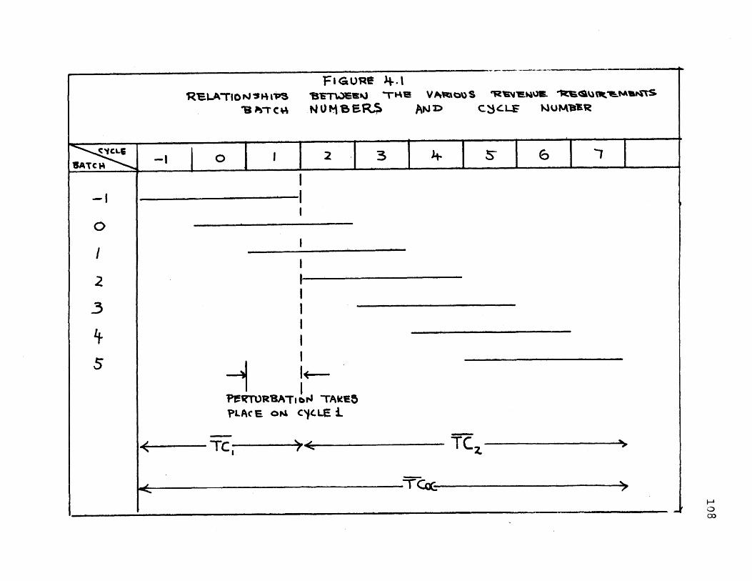
FIU'# 4.sRsLXriO o1 w sA v V Ava%) e ~u1vr-&mer
li tr c 44 N 0M -15F.P-.0
~Zi~E4 ~joj ij2 ~ I I 161~57
0
2
-3
4-C -p cc
Awm
1'WTSAT, b3rJ -TAIkEP~LACE 014 Cl(.LE:L
L-rT
-us-rumvEti -r§AlsCZ3<.LF WUM'DV-R

109Table 4.2
Comparison of Exact Incremental Cost with Incremental Cost
Calculated by Three Approximate Methods. ( No Income Tax)
Exact NuclideValue
Unit ConstantProduction Value
TU, Tu,QuantityCalculated
BatchesIncluded 7 3 3
(-1,o,1,2,3,4,5) (-1,0,1) (-1,0,1)3
(-1,0,1)
Revenue Reguirement
10$
SteadyState 62.3515
Additional Energy inCycle IAE =1029GWHt 62.7428
=2050WHt 63.1245
Part B.
25.8651 25.0157
26.2693 25.3782
26.6740 25.7430
Incremental Cost for Cycle 1
Mills/KWH
A E 1029GWHt
2050 GWHt
1.17
1,16
1.20
1.21
1.08
1.09
+ Mi1ls/kwhe=10ATC/10%AE.-
t *1 = thermal efficiency=0.326
Irradiation time =1.375 yearRefuelling time =0.125 year
Method
Part A
35.2680
35.9983
36.7316
2.18
2.19.

110of the objective function for batches -1, 0, 1, 2, 3, 4, and
5. The second, third and fourth. columns give the results
of calculation of the objective function by three different
approximate methods. For these columns, results are given
for only batches -1, 0, 1, since these are the only batches
whose contribution to the objective function are changed by
change of energy in cycle 1, under the assumptions of these
approximate methods.
The first row of Part A gives the objective function
for the stated number of batches for the unperturbed case.
The second row gives the objective function for an increase
in energy production AE in cycle 1 of 1000 GWHt, with un-
changed energy production in all following periods. The
third row gives corresponding information for an energy in-
crease of 2000 GWHt in cycle 1.
Part B gives incremental costs as defined in Equation
(4.13), for the two values of &E . The first column gives
exact incremental costs over the entire five cycles. The
last three columns give approximate incremental costs calcu-
lated by each of the three methods for evaluating the initial
and final inventories for the first cycle. These incremental
costs are calculated from Equation (4.13).
T TUM(E +AE1 ) - TCc( E )bt=E (4.13a)
AT-- T_(E +AE 1 ) - TC(E 1 )11 (4.13b)

111
From the results of Table 4.2, the Constant Value Method
clearly gives poor agreement with the exact values for the
incremental cost. Accounting for the changes in inventory
is necessary for calculation of the objective function in
periods of finite duration.
Both the Nuclide Value Method and the Unit Production
Method give incremental cost close to the exact value. Hence
both of them satisfies the equalized incremental cost condi-
tion of Equation (4.6). Since both of the methods are con-
sistent they can be accepted as a valid way to evaluate
changes in inventory value.
As mentioned under Section 4.3, the Unit Production
Method requires forecast of performance of future cycles. How-
ever, for these sample cases, the future operation of the
reactor after Cycle 1 has been explicitly specified. Hence
Table 4.2 a, b, show values of the objective function with
no forecast error.
In practical application of this method, when the future
is uncertain, the Unit Production Method may give less accurate
results for incremental costs due to uncertainty in future
discharge burnup and salvage values. Moreover, predicting
these values may increase computational effort to a large
extent. Hence, the Nuclide Value Method, which is consistent,
accurate in calculating incremental cost, and free from fore-
cast error, is recommended for calculating the objective
function for the case of no income tax.

1124.5 Objective Function Defined for the Case with Income Tax
4.5.1 Objective Function for the Indefinite Time Horizon
The objective function for the indefinite time horizon
is defined to be the "revenue requirement", which is given
by Equation (4.14).
b dwd (14.114)
where
Pwc Zib t present value of fuel cycle expenseswc (1+x) ib
wd f ib X wei6 E
discounted depreciation credit
Pb= T21 Eb t discounted electricity gener'atedwe (1+x) jb
b bE =LE total energy generated by batch b
ji3
T = income tax rate
For the derivation of Equation (4.14) refer to Benedict (&)
and Grant (G;). This definition of objective function is
consistent with the cost code MITCOST.
TC -Pwe

1134.5.2 Objective Function for the Finite Time Horizon
Objective function for the finite time horizon can be
derived in a manner analogous to the derivation in Section 4.2.
Again, it is necessary to introduce an inventory value for
those fuel batches that are in the reactor at the end of a
time period. Since depreciation credit is calculated for
each batch individually, an inventory value' must be assigned
on the per batch basis. Defining vb(t) as the residue value
of fuel batch b at time t , the objective function for the
finite time horizon is given by
IC 1 d -- 415)b
where the summation runs over all the fuel batches that have
ever been in the reactor during that time period.
For those fuel batches that are charged and discharged
from the reactor in thetime period, Pb P d are definedwc wd
earlier.
For those fuel batches that are in the reactor at the be-
ginning of the time period at time t1, but are not in the reac-
tor at the end of the time period
b V b(tT, Z ,PW =(1+x) I' . (1+x) i(
Pwd (t, + 2we (417)
e E
where 4 sum over expenses in this time period only
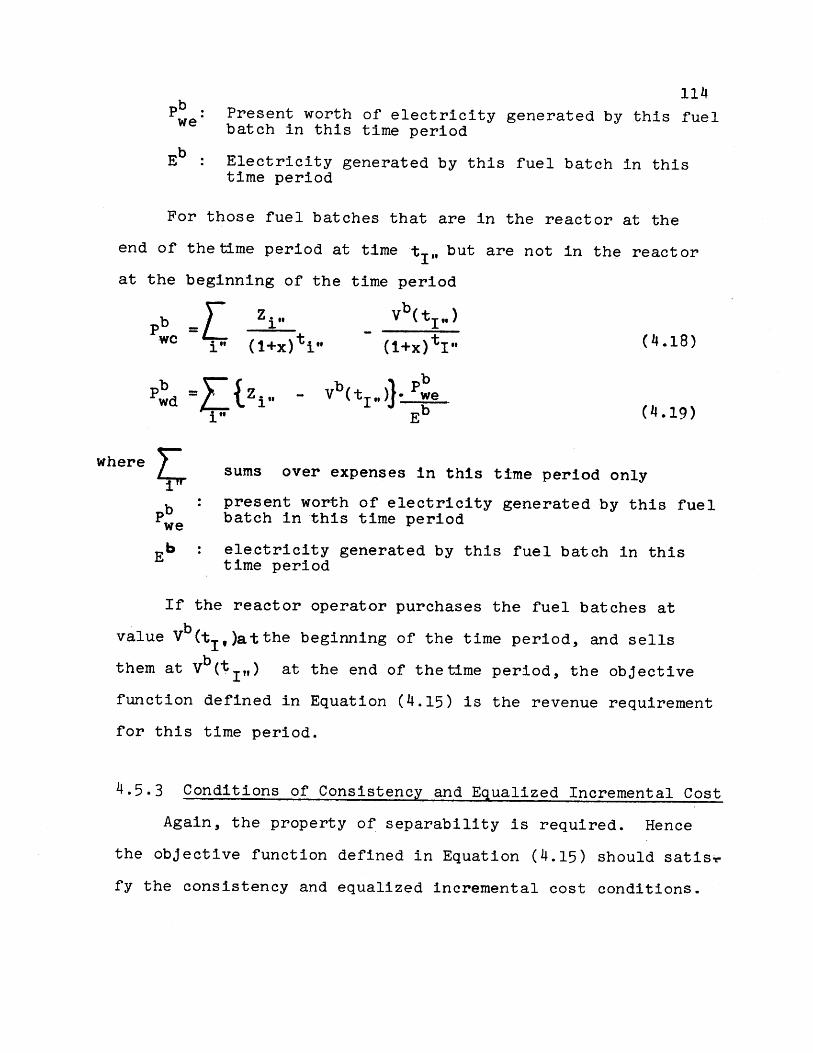
114P : Present worth of electricity generated by this fuelwe batch in this time period
Eb Electricity generated by this fuel batch in thistime period
For those fuel batches that are in the reactor at the
end of the time period at time ti,, but are not in the reactor
at the beginning of the time period
P b Z i , V b ( l)4 1WC is (l+x)tif - (1+x)tIl (4.18)
wd =tZi,, - Vb~t,).~e(.9" b (4.19)
wherewher sums over expenses in this time period only
b present worth of electricity generated by this fuelP we batch in this time period
Eb electricity generated by this fuel batch in thistime period
If the reactor operator purchases the fuel batches at
value Vb(t,)atthe beginning of the time period, and sells
them at Vb(t,11 ) at the end of thetime period, the objective
function defined in Equation (4.15) is the revenue requirement
for this time period.
4.5.3 Conditions of Consistency and Equalized Incremental Cost
Again, the property of separability is required. Hence
the objective function defined in Equation (4.15) should satis-
fy the consistency and equalized incremental cost conditions.

115
n
L c = (4.3)
n: number of time Deriods in the indefinite time horizon
~ ...(Tr . (14.6)9E c 3E
for those cycles c that are in time period I
Unfortunately, due to the effect of tax credits, it is
no longer possible to satisfy the consistency condition
exactly by imposing the equality of Equation (4.9).
Vb ( b f S - (14.9)(1+x) I" (1+x) (+i
Inconsistency comes from the fact that the depreciation
base for the finite time horizon case is different from that
of the indefinite horizon case.
Hence, the problem of separability reduces once again to
the problem of finding values of Vb(t) that come closest to
satisfying the consistency and equalized incremental cost
conditions.
Two different methods of evaluating Vb(t).have been exa-
mined. They are the Inventory Value Method and the Unit Pro-
duction Method. The Constant Value Method is not applicable
in this case because neglecting the relative changes of the
present value of fuel inventories is not consistent with tax
regulations.
4.6 Two Methods of Evaluating Fuel Inventories Vb
4.6.1 Inventory Value Method
Vb(t)is equated to the market value of nuclear material

116of fuel batch b at time t , plus the book value of fabrica-
tion and appreciated value of shipping, reprocessing, and
conversion. The value of the service cost is determined by
linear depreciation based on the Unit Production Method.
Vb(t1 ,) = $value (U,Pu) + $value FSRC
where $value FSRC = book value of fabrication, shipping, re-processing and conversion
(initial value-final value) fenergy=initial value . generated
total energy generation p to
initial value = ZF: fabrication cost
final value =-(ZS+ZR+ZC) : post-irradiation costs
Thus, $ value FSRC varies linearly with respect to energy
production from an initial value of the fabrication cost to a
final value equal to the sum of post-irradiation costs. Since
V b(t 1 ,) depends on the total amount of energy generated by
fuel in the reactor, projected into future operations, this
method is subject to forecast uncertainty. A forecasting
rule is given below in Equation (4.26) to project total energy
generation. No depletion calculations are involved.
Eb (N/n)- Eb (4.26)
Eb total energy generation for batch b
Ey : total energy generation up to time tI,
n :number of cycles the fuel batch has been in thereactor up to time
N :total number of cycles the fuel batch is expectedto go through before discharge
Since Eb and n are already known at time t1, , the onlyI
parameter to predict is N. Predicting N is much easier than

117
predicting Eb directly. This rule of thumb is useful when
very little or no information is available for predicting
the future. Even though this rule is crude, incremental cost
calculations based on the Inventory Value Method using this
rule of thumb give fairly accurate results (See Table 4.4).
If enough information is available to predict Eb reliably,
Eb should be used instead of this approximate value.
4.6.2 Unit Production Method
Vb(t) is equated to the book value of nuclear material
and service cost (FSRC) for batch b in time t . Book value
is determined by linear depreciation using the Unit Production
Method.
Vb(:t1 ,) = initial value of nuclides and FSRC
initial value of nuclides and FSRC otalnergy
- salvage value of nuclides and FSRC eneratio
Xtenergy generation up to tAwhere Initial value of nuclides, FSRC = 7U +ZF
Salvage value of nuclides, FSRC = ZU,+ZPu'ZS~ZR~ZC
In this method Vb(t ,) depends on both the total amount
of energy to be generated by the fuel in the reactor, projected
into future operations, and on the composition of the fuel
when discharged after these future operations. This requires
running depletion calculations. Hence, the depletion calcula-
tions must be carried out until all the fuel batches in time
period I have been discharged from the reactor. This would
provide enough data for calculating salvage value as well as
total energy. In order to complete the calculation for time

118
period I, it is necessary to predict system behaviour for
time period 2. This is much more difficult than predicting
E b and requires more computation effort.
4.7 Results of Two Sample Cases
The sample cases of Section 4.4 are used again to test
the degree of consistency and equality of incremental cost
for the two methods.
Similar to the treatment in Section 4.4, the objective
function TC. includes all seven batches (-1, 0, 1, 2, 3, 4,
and 5) affected by the perturbation. TO1 includes the first
three batches, credited with the inventory value of batch 0
and 1 at the end of cycle 1. TC 2 includes the last six
batches, charged with the inventory value of batch 0 and 1
at the beginning of cycle 2.
If the methods of evaluating inventory worth possess the
property of consistency, then T CeTc1+ TC . Hence,
any difference between TC cc and 7C1+T2 is a measure of
inconsistency for the two methods.
Part A of Table 4.3 gives the objective function for the
batches whose values are affected by changes in energy in
Cycle 1. The first column gives the result of exact calcula-
tion of the objective function for the indefinite time hori-
zon Tac . The second column gives the result of using the
Inventory Value Method for calculating the objective function
for time period 1, TO1 . The third column gives values of
TUC 2 . The fourth column gives the sum of TO 1 and TC 2
it should be compared with column 1. Part B is a similar table
for the Thit Production Method.

119
Table 4.3
Test of Inconsistency Between the Exact Value and the
Approximate Methods
Exact
Revenue Requiremert
Inventory Value Method
QuantityCalculated
Steady Statecase
Additional Energy inCycle 1AE,=1029GWHt
=2o5OGWHt
31.2713 44.9588
31.7532 44.9339
Revenue Requirement
Unit Production Method
QuantityCalculated
Steady Statecase
106$
75.8458 30.1342 45.7538 75.8879
Additional Energy inCycle 1AE10293WHt
=2050GWHt
76,3106 30.6041 45.7333
76.7661 31.0729 45.7073
76.3375
76.7802
Part A,
Method
75.8458 30.7900 44.9734
L6 t10w
76,3106
76.7661
75-7634
76.2301
76.6872
Method Exact

120
From the results in Table 4.3, the magnitude of incon-
sistency can be seen to be quite small for both methods in
all three cases, but the Unit Production Method in compari-
son has the smaller measure of inconsistency.
Table 4.4 shows the incremental cost for the two methods.
Incremental costs calculated from the Unit Production Method
give better agreement in general.
4.8 Conclusions
The Unit Production Method provides the most consistent
and accurate evaluation of V b(t). However, to use this method
in a practical cas.e, the information required as input is dif-
ficult to obtain. Moreover, more depletion calculations are
required.
On the other hand, the Inventory Value Method requires
the minimal amount of projections and computations, at some
loss of consistency and accuracy. For this kind of scoping
optimization which requires evaluation of many different al-
ternatives, computational speed is the major concern. Using
a fast optimization algorithm, a large number of cases can
be evaluated in order to eliminate those that are far from
optimal and locate those that may be optimal. Then a more
accurate algorithm can be used to evaluate those limited
number of near optimal cases.
Hence, the Inventory Value Method for evaluating V b(t)
is recommended for scoping calculation of the objective func-
tion for the finite horizon case.

121Table 4.4
Comparison of Exact Incremental Cost with Incremental Cost
Calculated by Two Approximate Methods
Incremental Cost for Cycle 1
Mills/KWHe
Method Exact Approximate
InventoryValue
UnitProduction
A E1=1029GWHt
=205OGWHt
1,39
1.38
1 .43
1,44
1040
1.40

122CHAPTER 5 .0
CALCULATION OF RELOAD ENRICHMENT ANDINCREMENTAL COST OF ENERGY FOR GIVEN
SCHEDULE OF ENERGY PRODUCTION WITH FIXED RELOADBATCH FRACTION AND SHUFFLING PATTERN
5.1 Defining the Problem
The problem here is to calculate the reload enrichments
and incremental cost of energy for successive cycles of a
particular reactor given the energy requirements for each
cycle and the refuelling schedule. The initial state of
the reactor is specified. Reload batch fraction and
shuffling pattern for each cycle are fixed. Under these
restrictive conditions, there is only one unique solution
for this problem. This can be understood quite easily by
analyzing the relationships between the variables.
If the initial state of the reactor is specified and
if the reload batch fraction and shuffling pattern for the
first cycle are fixed, the only refuelling option is the
reload enrichment. If the energy for the first cycle is
given, the reload enrichment for the first cycle is fixed.
This in turn specifies the end condition of the first cycle.
The above argument can be repeated for the second, third
and subsequent cycles. Hence, if the energy requirements
for successive cycles are specified there is only one
sequence of reload enrichments for this case.
The economics of the fuel cycle is a unique function
of the physical state of the fuel cycle. Since the physical
state of the fuel cycle is uniquely specified, the economics
of the system is also uniquely defined. Hence, incremental

123
costs for the various cycles can be explicitly evaluated.
5.2 One-Zone Batch refuelling case
For a batch refuelled one-zone reactor, the calculation
of reload enrichment and incremental cost of energy is
straight forward. Energy output depends entirely on the
reload enrichment for that cycle. There is no inter-coupling
between cycles.
Figure 5.1 shows the relationship between cycle energy
and reload enrichment for this one-zone case. For a sequence
of cycle energies, the sequence of reload enrichments for
successive cycles can be read off directly.
Since there is no inter-coupling between cycles, the
fuel costs for different cycles are also decoupled.
The objective function is given by
T = wc td (5.1)
= b Rb
L(1+x) tb
where P = revenue requirement for batch b
tb = irradiation starts for cycle b
The specific refuelling schedule is given in Table 5.1
Table 5.1
Refuelling Schedule (in years)
Cycle Irradiation Starts Ends1 0.0 1.4632 1.588 3.1513 3.176 4.6394 4.764 6.2275 6.352 7.815

124

125
Figure 5.2 shows the relationship between Rb and cycle
energy. For a given sequence of cycle energies, the sequence
of R bs can be read off directly.
The incremental cost of energy for Cycle c is equal to
the slope of the curve of Rb vs E curve. Notice that for
the same cycle energy, the incremental cost are different
for different cycles due to the present worth factor. Figure
5.3 shows the relationship between incremental cost and
energy per cycle.
Hence for the batch refuelling case, the reload
enrichment and incremental cost of energy for each cycle
can be calculated directly once the cycle energy and the
refuelling schedule are specified.
5.3 Multi-Zone Refuelling
In the more general case, only a part of the reactor
core is replaced during each refuelling. Energy generated
in any cycle originates from the fissioning of the fresh
reload fuel and the partially burnt fuel remaining in the
reactor. As a result, energy generated in one cycle depends
not only on the reload fuel for that cycle, but also in the
reload fuel for the preceding cycles. In this way, all the
fuel cycles are coupled together. Hence, the calculation of
reload enrichments and incremental cost is no longer straight-
forward.
Three methods are developed for the calculation. The
first method is the Rigorous Method based on the definition
of the incremental cost. The second method, called

126
.1.
'co C'YC,-E ENERrqy.
FOR FIVE SUCC EEDw4q2* VYCLES
IV'
AD'01
*TIMEJ
CYCLE ENERrx)f wIQ0 GWP
I

127
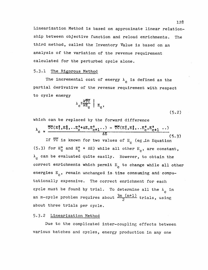
128
Linearization Method is based on approximate linear relation-
ship between objective function and reload enrichments. The
third method, called the Inventory Value is based on an
analysis of the variation of the revenue requirement
calculated for the perturbed cycle alone.
5.3.1 The Rigorous Method
The incremental cost of energy X is defined as the
partial derivative of the revenue requirement with respect
to cycle energy
c aE E ,c~ c
(5.2)
which can be replaced by the forward difference
TU(EO,El,..E+AE, E+1..) - n(E?,EO.,..E0 , E*+1XC -AE2
C(5 3__ (5. 3)If TC is known for two values of Ec (eg .in Equation
(5.3) for Ec and E0 + AE) while all other E , are constant,c c cA can be evaluated quite easily. However, to obtain thec
correct enrichments which permit Ec to change while all other
energies Ec , remain unchanged .is, time consuming and compu-
tationally expensive. The correct enrichment for each
cycle must be found by trial. To determine all the Ac in
an m-cycle problem requires about 3m 2(m+l) trials, using
about three trials per cycle.
5.3.2 Linearization Method
Due to the complicated inter-coupling effects between
various batches and cycles, energy production in any one

129cycle depends on the reload enrichments of all the preceding
cycles.
Ec = Ec (i, 2 ---- O) (5.4)
where iP is the initial state of the reactor prior
to Cycle 1.
For small changes of enrichments from a given base
case, the energy production per cycle can be approximated
by the linear relation
Ec -Ec_ -(c'~c*,) (5.5)where CO : reload enrichment for cycle c' for the base
case
E4 : energy production for cycle c for the basecase.
Equation (5.5) can be put in matrix form
= 4 AC + io (5.6)
where E = col {E 1 *... EC1
= lower diagonal matrix
E ( /Ac, for c' c
for c'> cAc = col{ACt........Ae}
= c21{ Ef..... E CSolving for A.C, Equation (5.6) becomes
+1 -1 + .+Ec = NA (E - E -) (5.7)
Adding C0 on both sides
+ +0 + 1 + +C = 0 + AC = A~ (E - E ) + 0 (5.8)
where c= col'{ ci... c
+0E col {E..g

130
If the elements in the matrix A are known, the reload
enrichments can be calculated for any specified set of cycle
energy.
A is lower diagonal. Equation (5.8) can be solved by
forward elimination.
The success of this method depends on the accuracy
-4 -4.of the elements of matrix A. If E is close to E or one
of the E's from which the coefficients are calculated, the
method can be very accurate.
The objective function TC for a finite time period can
be treated in a similiar manner. The objective function
depends on the physical state of the system, and consequently
it has the same set of independent variables.
TC = TC (E1-.. E 10) (5.9)
However, by the chain rule of differentiation,
C C,
3TC _ ET c_ L 3Ec' (5.10)c c
C!C
Equation (5.10) can be inverted to solve for c''
Rewriting Equation (5.10) in matrix notation
A\Tt (5.11)
where
T col. 3TC 3TC ........ 3 Ie DC1 3C2 acC
S = col. a 3_.... T-13E1 3E 2 aEC

131Inverting Equation (5.11) to solve for X,
=A\T)- fTc (5.12)
If matrix A\ and the vector are known,X can be
calculated directly.
The matrix A and the vector are determined by a
series of perturbation calculations. Using the steady state
case as the base line, the perturbed case consists of a
positive change in enrichment in the first cycle alone. Reload
enrichments for the succeeding cycles are kept to the original
steady state value. Cycle energy for the first few cycles
would be increased. This effect would slowly damp out. By
analysing the dampening effect in cycle energy, the elements
in matrix A can be determined.
For example
a -3E E1 (e+Acl) - E1 (d) (5.13)
a - = 2As (5.l13)11 Ac 1e
a _ 2 E2(e?+ het,,[ )-E e ,51)a21 3 1 (5.14)
aE5 E5(e*+Acj,eO....)-E5(ei'ei----a 51 Ac 5 (5.15)
Similiarly, 3T can be calculated.
DTC _TC(ei+Ae1e ... -TC(ei,E2*. .. ) (5.16)aei AE,

132Table 5.3 and Table 5.6 show the application of this
method in sample problem 1, 2 and 3.
5.3.3 Inventory Value Method
The Inventory Value Method consists of two parts. Part 1
deals with the calculation of reload enrichments by trial and
error. Part 2 calculates incremental cost of energy by
making use of the data generated in Part 1.
Part 1 Given an initial state of the reactor, the reload
enrichments for succeeding cycles for a specified sequence
of cycle energies can be determined by trial and error. This
method is primitive and costly, but it can be made as accurate
as one likes.
For a given initial state, a given requirement of cycle
energy, a guess is made for the reload enrichment for the
first cycle. A depletion run is made using the guessed value
for the reload enrichment. If the resulting cycle energy is
too high (low), the reload enrichment is decreased (increased).
The depletion run for this cycle is repeated. The cycle energy
for the adjusted reload enrichment is obtained. A third trial
on the reload enridhment can be made using interpolation, or
extrapolation based on previous results.
(1C) _ (i-1)(11 (i) (C -)
i)= Wi) (i-l) .(E(i) - EO) + E(i) (5.17)E -E
Where E0 = target valueE~i) = cycle energy for the i-th trialE(i) = reload enrichment for the i-th trial

133This method converges very rapidly. Usually three
trials of the enrichment are required for an accuracy of
+0.1%. With experience, the number of trials can be reduced
to two.
After the reload enrichment for the first cycle has
converged, the whole procedure can be repeated for the second
cycle.
For an m - cycle problem, at most 3m depletion runs are
required to determine the reload enrichments.
Part 2 Incremental costs can be calculated using data
generated in the trial and error procedures.
In Chapter 4, it has been shown that the Inventory Value
Method correctly evaluates the end effect and gives fairly
accurate values of incremental cost. If the Inventory Value
Method is applied at the end of the cycle for which incremental
cost calculation is desired, then incremental cost of nuclear
energy for that cycle can be obtained by analyzing the change
in the revenue requirement up to that cycle as energy production
changes in that cycle.
Consider the first cycle in the planning horizon in which
the initial state is well specified. After using the trial and
error procedures to calculate the correct reload enrichment
for the target energy, there would be at least three depletion
runs available for that cycle with different enrichments and
cycle energies.
From the output of the depletion runs, the revenue
requirement up to the end of Cycle 1 can be calculated for

134each enrichment or cycle energy. Incremental cost of energy
for the first cycle ATC can be approximated byAES
AYU TT,(EI) - TJ (El)
1 AE (E' - E")l1
Where El and El correspond to different trial energies for
the first cycle.
The same method can be applied for Cycle 2, 3... etc.
Hence, the incremental cost of energy for all the cycles can
be approximated.
From Equation (5.18) it may be noted that only two data
points are required for each calculation of incremental cost.
If more than two depletion runs are available for each cycle,
higher order coefficients can be calculated.
Figure (5.4) shows the relationships between YU, T1
(revenue requirements up to cycle 1) batches and cycle for the
example in which the incremental cost of energy for Cycle 1
is required.
5.4 Results For Three Sample cases
Three sample cases are considered in this section. The
first two sample cases deal with perturbation in a steady-
state operating condition. The third sample case deals with
non-steady state operating condition. The third case
supposedly is more realistic.
5.4.1 Sample Case 1 & 2
Sample Cases 1 & 2 are the same cases considered in
Section 4.4. The initial state of the 1065 MWe Zion type

RIELAT(Ob,.)'SHiPS 'BT---Twrv.Eo -viAut vARio%3s TRsvem%3B Rsekv3M mrM-TS
BATC" NUMBET;uS MCI> c S C L-F MST_l;t.
c L.E
SA-TCH
2
3
4
-Tcl
-j

136reactor is given by the steady-state operating condition of
three-zone, 3.16 w/o refuelling, with energy generation of
21935 GWHt per cycle. The energy production in Cycle 1
of the planning horizon is increased to 22964 GWHt per cycle
for case 1, and 23985 GWHt per cycle for case 2 by increasing
the reload enrichment. The energy productions in the
remaining cycles of the planning horizon are kept constant
at the 21935 GW1t level by adjusting the reload enrichments.
Table 5.2 shows the reload enrichments, cycle energies
and revenue requirementsfor the base line case and the two
perturbed cases. Incremental cost of energy calculated by
the three methods are presented in the last three columns.
The Inventory Value Method gives better results than the
Linearization Method when compared to the exact values given
by the Rigorous Method.
Table 5.3 shows the calculations required by the
Linearization Method. From a set of five enrichment
perturbation cases, the coefficients and - werec c
calculated. Solving the set of linear equations, the
incremental cost of energy - were determined, and areAEc
given in the last row of the table.
Finally Table 5.4 shows values of reload enrichment
calculated by trial and error and by the Linearization Method.
They agree within 0.3%.
5.4.2 Sample Case 3
This is a case with non-steady state initial condition and
varying cycle length and cycle energy. Refuelling intervals

Table 5.2
Incremental Cost of Energy for Sample Casese 1 and 2 Calculated By Three Different
Methods
Enrichment and Cycle Energy
E(w/o)E(GWHt)
RevenueRequirement
Incremental CostMethod of Calculation:Rigor- Inventory Linear-ous Value ization
Cycle 1
Base eCase E
Case 1 eE
Case 2 GE
3. 16221935
2
3.16221935
3 4 5
3.16221935
3.359 3.054 3.17422964 21935 21929
3.557 2.941 3.18623985 21919 21906
3.16221935
3.16221935
3.196 3.13321928 21933
3.235 3.10621937 21970
106r- Mills/kWHe69.983 -30.790
70.461 31.271 1,42
70.929 31.753 1.40'
1.43
1.44
1.37
1.37
Refuelling Time Schedule For These Two Cases
Irradiation starts
Years
0.0
1.53.04.56.0
Irradiation ends
1.3752.8754.375
5.8757.375
Cycle
1
2
34
5
HL'J

Table 5.3
Calculation of Incremental Cost Using the Method of Linearization for Sample Case land 2
RevenueEnrichment and Cycle Energy_
6(w/o)E(GWHt)
IncrementalRequirement Cost
__69 o6(bI) Mills/KWHeTMills/KWHtT
e 3,162E 21935 69.9837
Perturbation
Cycle 1 E 3.557
E 23985
A E/M, 5181.
Cycle 2 9 3.162
E 21935A E/M --
Cycle 3 A 3.162
E 21935AE/AE3 _
Cycle 4 f- 3.162
E 21935
A E/4% _-
Cycle 5 E 3.162
E 21935
3.162 3.162 3.162 3.162
23126 22424 21791 21929
3010. 1236. -364.71.5094
-15.
3.557 3.162 3.162 3.162
23985 23126 22424 21791
5181. 3010. 1236. -364.
3.162 3.557 3.162 3.162
21935 23985 23126 22424
5181. 3010. 1236.
3.162 3.162 3.557 3.162
21935 21935 23985 23126
_ - 5181. 3010.
3.162 3.162 3.162 3.55721935 21935 21935 23985
5181.
71. 3511
71.2338
70.9535
70.5965
3.8526 1.3646(0'4448)
3.4531 1.2408(0.4045)
3.1569 1.1176(0.3643)
2.4490 0.9178(0.2992)
1.5473 0.9163(0.2987)
-JLAJ
BaseCase
3.16221935
3.16221935
3.16221935
3.16221935

Table 5.4
Reload Enrichment Calculated By Trial Method and By Linearization Method
Sample Case 1
Cycle
Energy/Cycle
1
GWHt 22964.
2
21935. 21929.
Enrichment
Trial Method E(w/o) 3.359
Linearization e(w/o) 3.360Method
Sample Case 2
Cycle
Energy/cycle
1
GWHt 23985.
2
21919. 21906.
4 5
21937. 21970.
Enrichment
Trial Method e(w/o)
Linearization f(w/o)Method
4
21928.
5
21933.
3.054
3.046
3.174
3.181
3.196
3.191
3.133
3*132
3.557
3.55?
2.941
2.928
3.186
3.197
3.235
3.225
3.106
3.108
H

140
alternate between twelve and eighteen months. Cycle energies
follow a similiar pattern to the refuelling intervals. The incre-
mental cost of energy for Cycle 1 is obtained by decreasing energy
production in that cycle by 1000 GWH+ while keeping energy produc-
tion in other cycles the same as the base case. Table 5.5 gives
values of reload enrichments, cycle energies, revenue require-
ments and incremental costs. The accuracy of the Inventory Value
Method is comparable to the previous results. The apparent accuracy
of the Linearization Method is just coincidental.
Table 5.6 shows the calculations required by the Linearization
Method. The perturbation cases are the same as given in Table 5.3,
except that refuelling times are different.
Finally Table 5.7 shows the values of reload enrichment calcu-
lated by the trial and error method and the Linearization Method.
The same order of accuracy is obtained in this case as in the
previous two cases.
5.5 Conclusions
The Linearization Method is least accurate among the three
methods. However, once the coefficients are calculated, incre-
mental costs and reload enrichments for any cycles can be obtained
very easily. The Inventory Value Method is more accurate in terms
of incremental costs. However, the trial method of calculating
reload enrichments is awkward. Either the Linearization Method
or the Inventory Value Method can be used to estimate incremental
cost to be used in the beginning.

Table 5.5
Incremental Cost of Energy for Sample Case- 3 Calculated by Three Different Methods
Enrichment and Cycle Energy RevenueRequirement
e (w/o)E(GWHt)
Incremental CostMethod of Calculation:
Rigor- Inventory Linear-ous Value ization
Cycle
BaseCase
E
Changed r.Case
E
1 2
3.557 2.864
24105. 21532.
3.359 2.975
23085. 21535.
5 TC TC-10$-- Mills/KWHer
3.557 2.864 3.260
23621. 20999. 22172.
3.545 2.833 3.286
23605. 20995. 22164.
70.837 31.580
70.383 31.107 1.37
Error 4%
Refuelling Time Schedule For This Case
Irradiation starts
YeArs-
0.0
1.52.5
4.0
5.0
Irradiation ends
1.3752.3753.8754.8756.375
1.43 1.37
0.05%
Cycle
1
2
345
1H

Table 5.6
Calculation of Incremental Cost Using the Method
Enrichment and Cycle Energy
6 (w/o)E(GWHt)
of Linearization for Sample Case 3
RevenueRequirement
ATC/Ae IncrementalCost
BaseCase
E 3.162E 21935.
Perturbation
Cycle I r- 3.557E 23985.
AE/&e 5181.
Cycle 2 E 3.162E 21935.
AE/E. -
Cycle 3 6 3.162E 21935.
AE/Ae3 -
Cycle 4 6 3.162E 21935.
A E/helt -
Cycle 5 6 3.162E 21935.
69.59363.16221935.
3.16223126.3010.
3.55723985.5181.
3.16221935.
3.16221935.
3.16221935.
3.16221935.
3.16222424.1236.
3.16223126.3010.
3.55723985.5181.
3.16221935.
3.16221935.
3.16221935.
3.16221791.-363.
3.16222424.1236.
3.16223126.3010.
3.55723985.5181.
3.16221935.
3.16221935.
3.16221929.-15.
3.16221791.-363.
3.16222424.1236.
3.16223126.3010.
3.55723985.5181.
71.0973
70.9090
70.8707
70.5645
70.2515
3.8007
3.3248
3.2280
2.4542
1. 6631
1. 3687(0.4462)
1 1509(0.3752)
1.1647(0.3797)
0.8810(0.2872)
0.9847(0.3210)
I-j
--1 $ 0 4 mills/KWHe-10 - %ONO) Mills/KWHt

Table 5.7
Reload Enrichment Calculated By the Trial Method and by the Linearization Method
Sample Case 3
Cycle
Energy/cycle (GWH t)
Enrichment
Trial Method e(w/o)
LinearizationrE(w/o)Method
1
23085.
3.359
3.360
2 4
21532. 23605.
2.975
2-979
3.545
3.534
20995.
2.833
2.836
5
22164.
3.286
3.287
H-

144
CHAPTER 6.0
CALCULATION OF OPTIMAL RELOADENRICHMENT AND RELOAD BATCH FRACTION
FOR REACTORS OPERATING IN STEADYSTATE CONDITION AND MODIFIED SCATTER REFUELLING
6.1 Introduction
The problem of nuclear in-core optimization can be
formulated as follows: given a refuelling schedule and a
fixed energy demand, find the optimal combination of reload
enrichment and reload batch fraction such that the fuel
cycle cost is minimized. In this chapter, the special case
of steady-state operation is considered in which the size
of the irradiation interval and the energy demand are the
same cycle after cycle. Refuelling is done in a modified-
scatter manner. Fresh fuel elements are always put on the
outside annulus and once-irradiated fuel elements are scat-
tered throughout the inner core. Under these restrictive
conditions, the state of the reactor is uniquely defined,
as the reload enrichment and reload batch fraction are
specified. For a given combination of reload enrichment
and batch fraction, there is a unique fuel cost and a
unique cycle energy.
6.2 Mathematical Formulation of the Problem and OptimalityConditions
The problem of nuclear in-core optimization in the
steady-state case can be stated mathematically as

145
Minimize TO (ef) (6.1)
subject to constraints E(Ef) = E (6.2)B(c,f) < B* (6.3)
Where TO revenue requirement for a single cycleE :reload enrichmentf batch fractionEs :energy demanded by the system on this
reactorB* burnup limitations.
The revenue requirement for a single cycle is chosen to be
the objective function because in steady state conditions,
the revenue requirement for a single cycle is equal to that
of the succeeding cycles. Equation (6.2) is the constraint
that the energy demand must be satisfied. Equation (6.3)
is the limitation on discharge burnup.
Notice that for reactivity limited burnup, specifying
the cycle energy and reload batch fraction completely
determines the reload enrichment. hence cycle energy and
reload batch fraction can be taken as the independent
variables, and reload enrichment as the dependent variable.
Equations (6.1) (6.2) and (6.3) can be rewritten as
Minimize TO (E s ,f) (6.4)
Subject to constraints B(Es,f) <BO (6.5)
The non-linear Kuhn-Tucker optimality conditions for
Equations (6.1) and (6.3) are
BO - B(E sf*) > 0 (6.6)
f* 0 0 (6.7)
-. B(Es,f*)4 (Esf*) (6.8)
7 0 (6.9)
w(B0 -B(Es,f*)) =0 (6.10)
376 .f*+70B f* =0 (6.11)

146
Equations (6.6) and (6.7) state that at (Es, ) the burnup
constraint is satisfied. Equations (6.8) and (6.9) state
that at (Es, * ) the objective function cannot be further
minimized. Equations (6.10) and (6.11) state that either
(Bo - B(Es, f ) )is zero or is zero. Physically thatY af
means the optimal solution(E s, f )either lies on the boundary
of the constraints, or it is at a local minimum. Combining
Equation (6.8) and Equation (6.1) reduces to
(Es, f 3 B(Esf (6.12)a f - - fg( .2
For steady-state refuelling, the average discharge
burnup B(Es, f) can be expressed in analytic form, in terms
of the cycle energy Es and reload batch fraction f
B(Es, f) . W * f = Es (6.13)
or B(Es, f ~ (6.14)
where W is the mass of uranium for the entire core before
irradiation.
Substituting Equation (6.14) into Equation (6.10) results in
=- 0 (6.15)
If the maximum allowable burnup is high eg. B0 > 60
MWD/kg, Equation (6.6) would never be zero in the practical
range Es.
Hence, according to Equation (6.10) n would be zero.
In this case, the condition at optimum would be
3TC (Esf*) 0W~ ~ (6.16)

147
However, if the maximum allowable burnup is low, eg.
BO < 30 MWD/kg, w is not equal to zero, and hence
BO - E /(W.f*) = 0 (6.17)
f*= Es/(W-BO) (6.18)
At these lower maximum allowable burnups, the optimal batch
fraction can be expressed as a linear function of (ES/B*).
6.3 Graphic Solution for Optimal Batch Fraction
A direct way of solving this problem is to calculate TC
for all possible choices of Es and f. Since TC is a smooth
varying function of these variables, calculating TC on a
coarse mesh of Es and f would give an adequate representation
of the function. Results shown on Table 6.1 are based on the
Zion type 1065 MWe Pressurized water reactor. Figure 6.1
shows TC versus Es for various values of f.
In Fig. 6.2, revenue requirement has been replotted against
batch fraction at constant cycle energy. In addition, lines of
constant average burnup B* are plotted. Only the region to the
right of a line of constant burnup is compatible with the
burnup constraint (6.3).
At the higher cycle energies of 10,650, 9,000 and 7,500
Gwhe, with a burnup constraint of 30 MWD/kg the optimal batch
fraction occurs at the intersection of the constant burnup
line and the constant energy line. At the lowest cycle energy
of 5,000 Gwhe, the optimal batch fraction occurs at the
lowest point on the constant energy line, at which condition
(6.16) is met.

148
Table 6.1
Table of Revenue Requirement Per CycleEnergy Per Cycle
and Average Discharge Burnup versus Batch Fraction and
Reload Enrichment
Batch 1/1Fraction ___
1/2 1/3 1/4 1/6
Enrichment
TC 17.8372.0 E 6278.
B 8.879
TC 21.2242.4 E 9259.
B 13.097
TC2.8 E
B
24.71212127.17.155
T 28.2723.2 E 14906.
B 21.085TCd
3.6 EB
TfC4.0 E
B
4.4 EB
4.8 EB
5.3 EB
7.0 EB
TU (10 6 $)E (GWHe)B (MWD/Kg)
10.7984287.12.129
12.8796092.17. 23515.0157801.22.068
17.1929441.26.708
19.39911032.31.209
21.62912577.35.58223.8801089.39.861
10.0575311.22. 539
11.5956026.25.571
13.2787251.30.771
14.9828434.35.79116.7009575.40.634
18.43010687.45.352
20.17411775.49.968
9.7994938.27.93811.2365959.33.71812.6686899.39.03514.1227827.44.285
15.5838720.49.339
17.0529593.54.27718.90110660.60. 316
9.0654348.36.90710.2325053.42.889
11.4045730.48.635
12.5856385.54.19513.7697019.59.564
N.A.
20.33910253.87.021

149
RV 6.1 -- - --
-~ VS C YCLG~ t7/ERGY /- FcOR -----
VARIOUs a3ATca t-A4CTION3
S* -.--- -- 4
0N7
* _ _ _ .. 07
r~ * _. .' __
Qz4
a, C,----
iv.----
'5,
3CA 72839
C yCL=j/2G i \/ O' G14W0
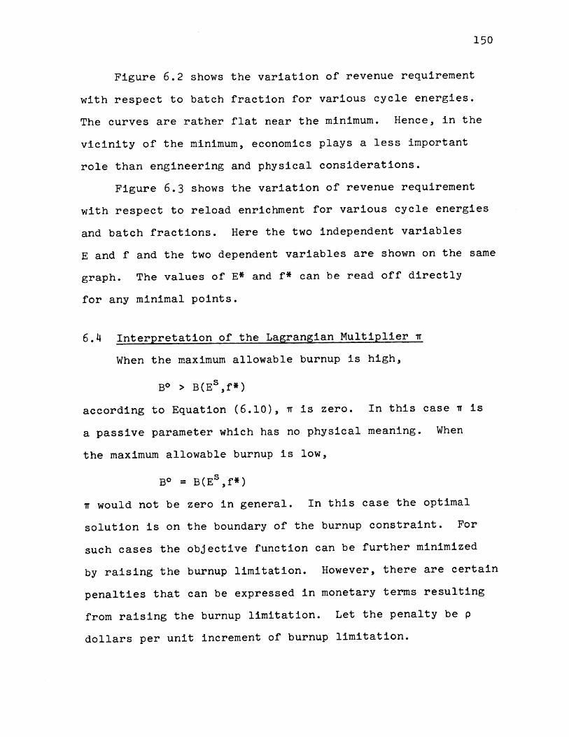
150
Figure 6.2 shows the variation of revenue requirement
with respect to batch fraction for various cycle energies.
The curves are rather flat near the minimum. Hence, in the
vicinity of the minimum, economics plays a less important
role than engineering and physical considerations.
Figure 6.3 shows the variation of revenue requirement
with respect to reload enrichment for various cycle energies
and batch fractions. Here the two independent variables
E and f and the two dependent variables are shown on the same
graph. The values of E* and f* can be read off directly
for any minimal points.
6.4 Interpretation of the Lagrangian Multiplier 7t
When the maximum allowable burnup is high,
BO > B(EsIf*)
according to Equation (6.10), n is zero. In this case n is
a passive parameter which has no physical meaning. When
the maximum allowable burnup is low,
B* = B(E sf*)
n would not be zero in general. In this case the optimal
solution is on the boundary of the burnup constraint. For
such cases the objective function can be further minimized
by raising the burnup limitation. However, there are certain
penalties that can be expressed in monetary terms resulting
from raising the burnup limitation. Let the penalty be p
dollars per unit increment of burnup limitation.

151
Ftc-. 6.2 ?2VENUE REQUiREN VS
BATCrt F=- AC -1tO /=Fo P / FP.Q ENTLL=.L.S 1=A/JRGV
L = //?RR ADlAT10 PLFFCDC-AZP4r CT Y 1~-ACro
-~~ tRRF~ADIATaCnV ;Ar-ERVAL1, 3 75 V&iS
RFU-EL-.'Gn- S1if )DC WN
0. Ot 3BATCH FRACTIO
I.C,

152
FIGURE 6.3
REVENUE REQUIREMENT VS RELOAD
ENRICHMENT FOR VARIOUS LEVELS OF ENERGY
C,
/1 $
/6/
/2
cN
~~'),I~ Ca I /100,---~-
~ / ; 7'~RICD CAPACITf iZACOR~
375~YR?. IiR~AD. I/WI eiF'VAL/O - i o. v. I-UmA/s- nw=-
Kf EVJ' /Ct H MIL/NT tV'/O
2 3 + 6bL0 7

153
Decreasing batch fraction by 3f would result in a saving
0 DTC(Esf*). af dollars
af 3B(Es f)If this saving is more than the penalty p- aE * af
there would be an incentive for decreasing the batch fraction
further. The penalty p* for which one is indifferent to
decrease or not to decrease Df is
3DTU(Es,f*) . aB(Esf*) (6.19)af a
Since > 0 according to Equation (6.8) and < 0,*
p would be negative, meaning that it is a penalty. Comparing
Equation (6.19) with Equation (6.12) reveals that
i = -p (6.19)
Therefore, one can interpret n as the maximum price one
would be willing to pay to increase the maximum allowable
burnup.
6.5 Calculation of Incremental Cost of Energy X
Since the objective function TC and the constraints
BO > B are functions of two variables, cycle energy Es and
batch fraction f*, defining incremental cost deserves
special attention.
Let f* be the optimal batch fraction for the problem
minimize TJ(Esf) with respect to f
subject to constraints BO>B(ESf)
Let ft be the optimal batch fraction for the problem
minimize TU(Es + E,ft) with respect to f
subject to constraints BO>B(Es + AEf)

154
Incremental cost of energy is defined formally as X where
X = limit T(Es + AE,ft) - TU(EsAE
AE+O (6.21)
This equation can be simplified for the following two
special cases.
Case (a): The maximum allowable burnup B* is very high,
such that BO > B(ESf*)
B4 > B(Es + AE, f )

155In this case r = 0 according to Equation (6.10). Therefore
according to Equation (6.11)
3TC(Es =0 (6.22)af
3TC(Es + fEft) =0 (6.23)
Equation (6.22) and Equation (6.23) could be solved
individually for f* and f+. Substituting f* and f into
Equation (6.21) would yield the incremental cost of energy A.
Case (b): The maximum allowable burnup B4 is low, such that
B4 = B(Es 2f EsW-f
B* = B(E5 + AE, f +) Es + AE
W.f
* ES 624or f = (6.24)
W-B
+ Es + AE (6.25)
W-B
Substituting f and f into Equation (6.21) would again yield
the incremental cost of energy A. Note that in any case,
incremental cost of energy A is not given by the partial
derivative of total cost TC with respect to cycle energy E
holding batch fraction f constant, but is given by Equation
(6.21) with the f and f+ determined by either Equations
(6.22) and (6.25) or Equations (6.24) and (6.22)
Figure 6.4 shows incremental cost of energy A versus
cycle energy E5 for various burnup limitations. For the same
cycle energy Es, incremental cost of energy increases with

156
Figure 6. 4
INCREMENTAL COST X VS
CYCLE ENERGY FOR VARIOUS BURNUP LIMITS B0
7EYCILc-5NEGY //\V
9103 GwHe
L- /0 //
C YCL4E

157.
decreasing allowable burnup levels. When the burnup constraint
is not controlling, incremental cost first increases, then
levels off with increasing cycle energy.
6.6 Effects of Shortening the Irradiation Interval
Fuel cycle calculations are repeated for refuelling
interval of one year based on the same depletion calculations
given in this chapter. The results are shown on Figures 6.5
and 6.6.
The following differences can be seen between the cases
of 1.5 year and 1 year refuelling interval. The revenue
requirements for all cycles are lower for the 1 year case.
This is due to a shorter time period in which carrying
charges are based. The optimum batch fraction for a given
cycle energy is somewhat lower. But the overall trends of
the two cases are very similar. Hence, for small variations
of refuelling interval, the behavior of the incremental cost
and optimal solutions would not be greatly changed.
6.7 Conclusions
For steady-state refuelling, the problem of nuclear
in-core optimization can be solved directly by graphic
techniques. For a specified cycle energy, the optimal batch
fraction is given by the smallest value compatible
with burnup limitation for nearly all practical cases.
The explanation is that the savings in service components

158.

159.

160

161In this case fr = 0 according to Equation (6.10). Therefore
according to Equation (6.11)
3TC(Es =0 (6.22)af
aTC(Es +M.E,ft) =0 (6.23)
Equation (6.22) and Equation (6.23) could be solved
individually for f* and f+. Substituting f* and f+ into
Equation (6.21) would yield the incremental cost of energy X.
Case (b): The maximum allowable burnup BI is low, such that
BI = B(Es ) = EW-f
B* = B(Es + AE, f+ ) E5 + AE
W-f
* Eor f = (6.24)
W-B
+ E + AE (6.25)
W-B
* +Substituting f and f into Equation (6.21) would again yield
the incremental cost of energy X. Note that in any case,
incremental cost of energy X is not given by the partial
derivative of total cost TC with respect to cycle energy E
holding batch fraction f constant, but is given by Equation
(6.21) with the f and f+ determined by either Equations
(6.22) and (6.25) or Equations (6.24) and (6.22)
Figure 6.8 shows incremental cost of energy X versus
cycle energy E for various burnup limitations. For the same
cycle energy Es, incremental cost of energy increases with

162
4-1
FlauRt 6.8INCR.EMENTA .. Cc5ST
'-'3
I~u~Jj
& ~oR1A ~iQUS
1OR te uP LIt4Y"T
A --IP.wA~A
2ap
i'p2
RET-091- I irq- 125
S BO
TINE
CAl AC~T~~ 'WAc~ovft i2
-1.0 b ba-ills c
Ltoi
M14
~1~* I* --V.---,.
10 mt(a.
2.14-
-

163decreasing allowable burnup levels. For the same burnup,
incremental cost first increases, then levels off and
finally decreases for increasing cycle energy.
6.6 Effects of Shortening the Irradiation Interval
Fuel cycle calculations are repeated for refuelling
interval of one year based on the same depletion
calculations given in this chapter. The results are
shown on Figures 6.9, 6.10, 6.11, 6.12.
The following differences can be seen between the cases
of 1.5 year and 1 year refuelling interval. The revenue
requirement for all cycles are lower for the 1 year case.
This is due to a shorter time period in which carrying
charges are based. Incremental cost of energy shows a
wider spread for the range of burnup limits considered.
But the overall trends of the two cases are very similar.
hence, for small variations of refuelling interval, the
behavior of the incremental cost and optimal solutions
would not be greatly changed.
6.7 Conclusions
For steady-state refuelling, the problem of nuclear
in-core optimization can be solved directly by graphic
techniques. For a specified cycle energy, the optimal
batch fraction is given by the smallest value compatible
with burnup limitation for nearly all practical cases.
The explanation is that the savings in service components

I
164
Nil I/44-V-i-4-11411T7 F - I - 2Z~i17zLL - -
2 I*1
4
qI
]-4-- 1-K WKKLJJ~LLLILLhi
I I 1 t - 1-1 - I - -4 -54 - - -
9I./
*~q1 ~
Al
AJ~Y!~:i~irv
I/lA'
OF.I... .i.i..I
___ I ___
p4 -
-T0
7-777 -
p1
1N .. . -4
_ _ i . .OF/O
* _ I
71i17C --- I
~fT~777f
* I
I-i-i
K -
ii*1
4-
lit-T 1 I -t -- ± 1-4- - -T - 4- -4- -4--Lt
~f7K49
/
-17
-A--
T
r---7
-J
e
L4 Tmny-.Vl r- IV r. KA PIC

165

166

167
-. d - W-6- fo
- m -mo
-yr
RE M7RL COS7T 7th
2RA 1DIA-rIoC 11N"MRVML
i
C~IC.L~ 1~g
I0a
p q
p4a A sat
pit IC'1
I VAPI
II
I I-
~~~c-ro~jC I
m -3
MOI.I
1.06.412S O~h1I~O.R1 cow

168
costs resulting from a smaller batch fraction outweights
the additional enrichment cost, carrying charges and
income taxes. Finally, the incremental cost of energy
increases with cycle energy, but levels off at E ~ 10,000
GWHe/cycle. The incremental cost of energy also increases with
decreasing allowable burnup levels.

169
CHAPTER 7.0
NUCLEAR IN-CORE OPTIMIZATION FOR NON-STEADY STATE
FORMULATION OF THE PROBLEM
7.1 Introduction
Having solved the steady state nuclear in-core
optimization problem in Chapter 6, this chapter considers
the general non-steady state nuclear in-core optimi-
zation problem outlined in Chapter 2 Section 2.5. The
general problem of nuclear in-core optimization can be stated
as follows: given a refuelling and maintenance schedule,
and a specified sequence of cycle energy demand for a
given reactor in the planning horizon, find the optimal
combination of reload enrichments and batch fractions such
that the fuel cycle cost is minimized and the engineering
constraints are satisfied. A typical planning horizon
consists of five cycles with a total duration of about
seven years. In general the cycle energy demand for each
of the five cycles would be different from each other.
Consequently, the reload enrichment and batch fraction for
each cycle would be different and hence the reactor supp-
lying this energy is said to be operating in a non-steady
state manner. At the beginning of the planning horizon,
the reactor is in a certain well specified initial state.
This initial state would play an important role in the
overall optimization. In addition to satisfying the cycle
energy demand, the optimal combination of reload enrich-

170
ments and batch fractions should also satisfy engineering
constraints, such as burnup limitations, power peaking,
control poison margins and other safety considerations.
Only when all these constraints have been satisfied does
the economics optimization has any practical significance.
7.2 Mathematical Formulation of the Problem
For full-power reactivity-limited burnup, cycle energy
and discharge burnup are unique functions of the reload
enrichments and batch fractions of all the preceding cycles.
Hence, reload enrichments and batch fractions can be con-
sidered as independent variables, while cycle energy and
discharge burnup can be considered as dependent variables.
The objective function: revenue requirement for the plan-
ning horizon, is also a variable dependent on reload enrich-
ments and batch fractions.
Thus, the problem of non-steady state in-core optimi-
zation can be mathematically stated as
minimize T (7.1)
with respect to I and
subject to constraints
E (,1J )=Es (7.2)c c
Bc ((7 (7.3)
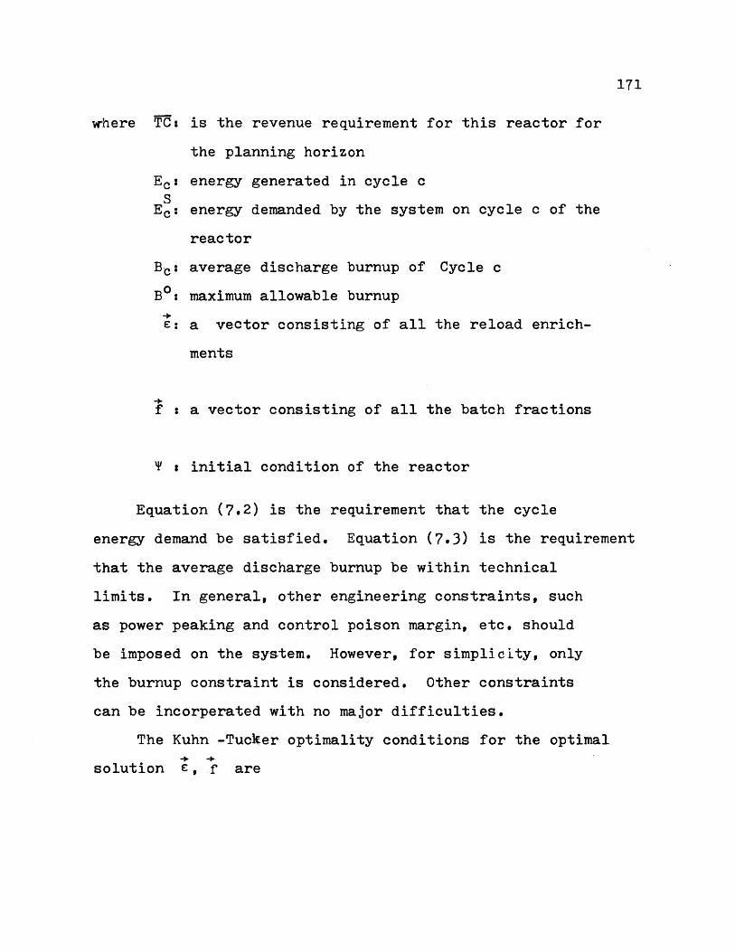
171
where Td: is the revenue requirement for this reactor for
the planning horizon
Ec: energy generated in cycle cS
Ec: energy demanded by the system on cycle c of the
reactor
Bc: average discharge burnup of Cycle c
B0 : maximum allowable burnup
E: a vector consisting of all the reload enrich-
ments
f : a vector consisting of all the batch fractions
T : initial condition of the reactor
Equation (7.2) is the requirement that the cycle
energy demand be satisfied. Equation (7.3) is the requirement
that the average discharge burnup be within technical
limits. In general, other engineering constraints, such
as power peaking and control poison margin, etc. should
be imposed on the system. However, for simplicity, only
the burnup constraint is considered. Other constraints
can be incorperated with no major difficulties.
The Kuhn -Tucker optimality conditions for the optimal
solution E, f are

Ec(S*,T*)=E
B c('C*,*)<B"
for all c
1*>0
C Sa Z{w e(B'-B )+Xj(E -)}3TC3e c c c c c -e
C
C S-a X{wg(B 0 -Bc)+x (E E ))x3T
Tc CC C
C
c * \(E -Ec =0
172
(7.4)
(7.5)
(7.6)
(7.7)
(7.8)for all c'
for all c' (7.9)
(7.10)
C C C{ 3TxC +9 xf*}= I Cx ( -Ife(80-Bc)+X;(E S-Ec
c '5cTc c c dT- c c cc
(7.11)C C
+ c T~ X{wy(BO-B )+AXj(E -Ecc c c
where Xc is defined as the incremental cost of nuclear
energy for the c-cycle
7 : is defined as the burnup penalty for the c-cycle
Since the dependent variables are not analytically
differentiable, the optimality conditions are not useful
in a practical sense. Calculation of the incremental
cost and burnup penalty directly from these equations is
not feasible.

173
Methods of solving the nuclear in-core optimization
problem are given in Chapters 8 and 9. Calculation of
incremental cost is given in Chapter 9 .
7.3 Exact and Approximate Calculation of the Objective
Function
The objective function TCI is defined as the revenue
requirement for the reactor in the planning horizon I.
The method of calculating TC is given in Section 4.3.2,
with end state correction based on the Inventory Value
Method. In principle, it includes the revenue requirement
for all the batches discharged from the reactor in the
planning horizon. The treatment for these batches is
exact.
Those batches that remain in the reactor core at the
end of the planning horizon are assigned a value Vb (00
that reflects the nuclide value and residual book value of
fabrication, shipping, reprocessing and conversion.
For these batches, the calculation of revenue require-
ment is only approximate because of these service costs.
Hence, the accuracy of the approximate TC is compared
to an exact revenue requirement TCc based on a pre-specified
fuel strategy. The number of batches included
in TCI and TCa are shown schematically in Figure 7.1.
The result of the test would hopefully demonstrate that
optimization based on the approximate TCI is equivalent

A~c
-I A
AA
A I03O r Fr- N m-r-tCl-r3s q3f~r cp IUL Vl lAv4.-bI A .l 5cL

175
to optimization based on the exact TCw..
If e* and "* is the optimal solution based on an
exact calculation of da., according to Kuhn-Tucker opti-
mality conditions Equations (7.8), (7.9) and (7.11) would be
> {wc(B -B(c c(E) - E
(7.12)
C(3 {( (B"-B (Z*,J*))+ A (ES- Ec (
Bfc'c'4 e c e (7.13)
C .C. C
CCI~~ec~w c cTCCCJ)C. E-E)QL I** X
@(7c(B 0-Bc)+X (E c
(7.14)
+ If'ewj-;y *(0 B)Xd(Ec E)C CC CCC
C+ C (7c(BI-Bc)+ ( c
However, if one requires $*, f* to be the optimal
solution based on the approximate objective function TdI,
*, 7* should also satisfy the Kuhn-Tucker optimality
condition for TI. Hence, the Kuhn-Tucker conditions for
e* ,f* and TCI are exactly similar to that of Equations
(7.12), (7.13) and (7.14) with TO1 replacing TCc. . Since
the right sides of the equations are not affected by the
replacement, the value of the left hand side of the equations
should be the same for TCI and TCO . In other words, we
should show that

176
3___.(_*,_ 37I 9T , (c *, *) (7.15)
3 -. , a_ ( , (7.16)af c a e
Therefore, if each partial derivatives for TCW. is
equal to the corresponding derivative of TO1 , then optimi-
zation based on either of them is equivalent.
7.4 Comparison of the Exact and Approximate Methods
The partial derivatives of TOI are compared to those
of TC, in a series of sample cases.
Planning horizons for each of the sample cases con-
sist of five cycles. However, to calculate TC it is
necessary to know the reload enrichment and batch fraction
up to the eighth cycle. The reload enrichinents and batch
fractions. for the sixth, seventh and eighth cycle are taken
to be 3.2 w/o and 0.33 respectively. Calculations are
based on the Zion type 1065 MWe PWR. At time zero, the
reactor is down for refuelling after it has been refuelled
in a three-zone modified scatter manner with 3.2 w/o reload
enrichment until steady state has been reached. The energy
requirement for each of the next five cycles is 22750 GWHt.
The maximum allowable average discharge burnup is 32 MWD/kg.
Under these restrictive conditions, the optimal reload
enrichments and batch fractions are E=3.2w/o and f=0.33 for

177
the next five cycles. In other words, the reactor is already
optimized before the planning horizon.
The reload enrichment or the batch fraction for the
first cycle is varied in order to evaluate the partial
derivative of the objective function with respect to enrich-
ment or batch fraction. The partial derivatives for TCoWare
TC T f+, !....) - U(19 ... ) (717)
-- tfe§ (7.18)
Partial derivatives for TOI are similiar to Equations (7.17)
and (7.18) by replacing TCw with TCI.
Figure 7.1 shows schematically the number of batches
included in TCI and TCw, the last three of which bring
the reactor sufficiently close back to steady state condition.
TC6consists of eight batches irradiated from Cycle -2 to
Cycle 8 for a total of eleven cycles. TCI consists of the
same eight batches irradiated from Cycle -2 to Cycle 5 for
a total of eight cycles, with the last three batches given
approximate ending inventory value based on their discharge
composition and burnup. Table 7.1 shows the values of TO1
and TCoc for the optimal case and the cases in which reload
enrichment or batch fraction is varied. Figure 7.2 and Figure
7.3 show the value of TC and TC. plotted against E1 and
f1 respectively.
The accuracy of the partial derivatives on E1 is within
+ 0.6%. The accuracy of partial derivatives on f1 is within
± 0.9%. The accuracy of partial derivatives onE29 E 3 .and

178Table 7.1
Exact and Approximate Revenue Requirements
for Various Enrichments and Batch Fractions
Enrichment(w/o)
S1 E 2 53
3.2 3.2 3.2
2.0 3.2 3.2
2.8 3.2 3.2
3.7 3.2 3.2
4.4 3.2 3.2
3.2 3.2 3.2
3.2 3.2 3.2
3.2 3.2 3.2
EnrichmentChanges
(w/o)
-1.200
-0.434
+0.480
+1.200
BatchFractionChangesAf-0.8
-0.4
+0.4
Batch Fr
4 53.2 3.2 0.3333.2 3.2 0.3333.2 3.2 0.333
3.2 3.2 0.333
3.2 3.2 0.333
3.2 3.2 0.253
3.2 3.2 0.293
3.2 3.2 0.373
0.333
0.333
0.333
0.3330.333
0.3330.3330.333
0
0
0
0
0
0
0
0
Revenue RequirementChanggs
ATC I ATCa-4.5720 -4.5804
-1.6648 -1.6746
+'.8893 +1.8791
+4.6642 +4.6542
Revenue RequirementChanges
ATC 106$ A
-2.a3i4 4 -2.3423-1.1717 -1.1822
+0.7716 +0.7658
action Revenue Requirement
f3 f4 £5 Approxi- Exactmate 106$
.333 0.333 0.333 87.6426 93.506
.333 0.333 0.333 83.0706 88.9801
.333 0.333 0.33 85.9778 91.8859
.333 0.333 0.333 89.5319 95.4396
.333 0.333 0.333 92.3067 98.2147
.333 0.333 0.333 85.2932 91.1982
.333 0.333 0.333 86.4709 92.3783
.333 0.333 0.333 88.4142 94.3263
A1C-/As1 AT-c/C
3.81003.8360
3.93613.8868
3.81693.85863.91483.8785
A 1 /A f1 A_ /Af
10 6 1
2.93672.92931. 9290
2.9528
2.9554
1.9146
Error
+0.2
+0.6
-0.5
-0.2
Error
+0.5
+0.9
-0.7

VAR IATIONJ OF
IC - AN 0 Yi~or
WLAITh IR5'PECT
FiNITE PLAxmMIIc
mr ...1,QR IMM4e,4T
I,4bpIrrK1MieT4I
TICmCo~
U
-lEo -g ~ -S.'. ~
.1
A~c (/O)
179
.1 64 a ro V gop
.- 2
-.3
2.
t
I.54 ~ -v 5' ~,
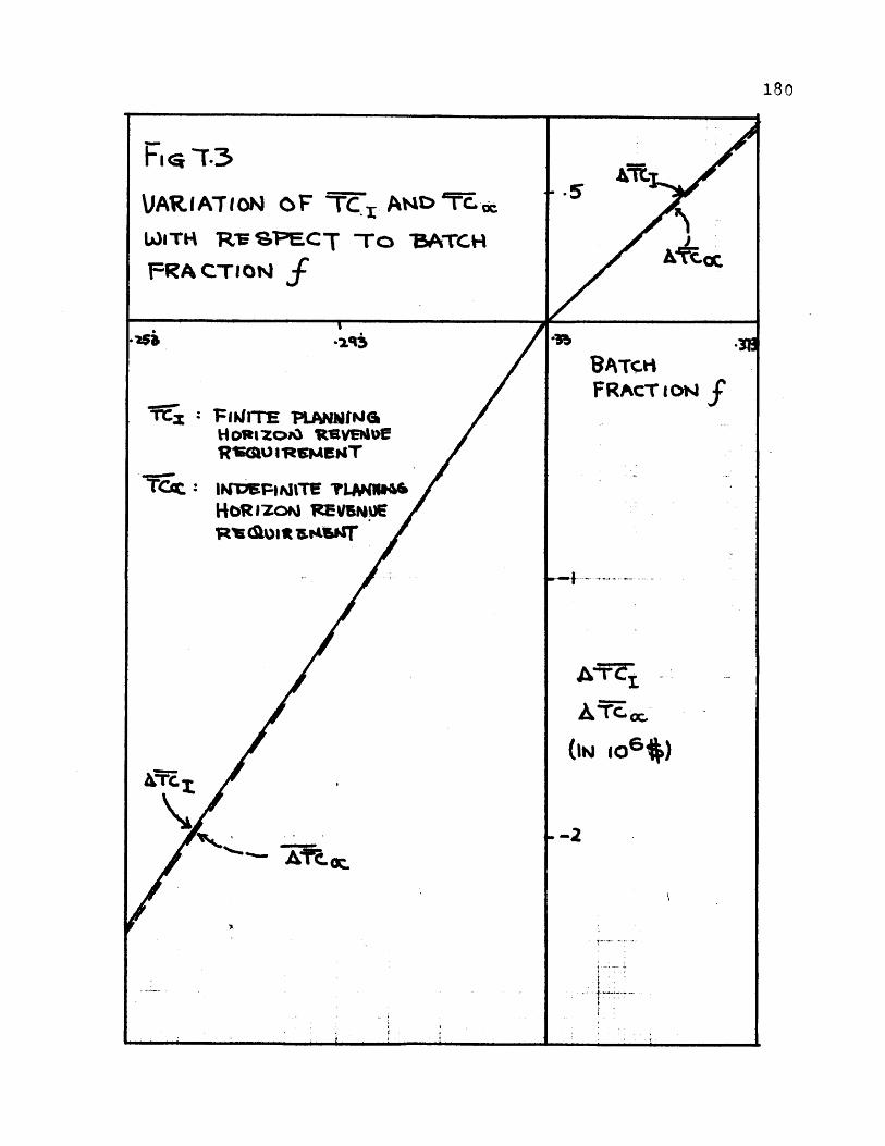
VARIATICOF CP7. AND.LieTH STECT Tro 'BATCH
T--ACTlONf
T T: uTrr PLAWNGJ
HtORIZON) REYEI4E
RWU cMN
IfFgA~EA4S
VA-M~kiFRAcT i c*4
ATT.Ti
(Ow lot
* 1-----
180
$314
S
I 1-

181
f2'''f5 would be progressively worse. This is due to the fact
that the end state correction would have a larger effect on the
subsequent cycles. However, this optimization would be
repeated on an annual basis. Hence, it is only the first
cycle results that would actually be utilized. Therefore, the
main emphasis on accuracy would be placed on the first cycle
derivatives.
This degree of accuracy is adequate for a survey type
of calculation in which a large number of cases are analysed.
After eliminating most of the sub-optimal cases, the exact
objective function would then be used for the final optim-
ization.
As a final test, the values of TO1 and TCe are calculated
for a complicated case in which the reload enrichments and
batch fractions are different for all the cycles. The
difference of TOI between this complicated case and the
optimal base case in the preceding sections is compared to the
same difference for TCU. Table 7.2 shows the value of TI and
TCco for the two cases. The discrepancy in this case is
substantially larger. This is due to the fact that as
enrichment and batch fraction changes take place near the end
of the planning horizon, the end-effect correction would not
be able to handle these changes accurately. Nevertheless,
this serves the purpose of comparing TOI and TCO under the
worse possible situation.

Table 7.2Exact and Approximate Revenue Requirement Calculated for the Base Case and the Case in
which the Reload Enrichments and Batch Fractions for All the Cycles are Changed
Cycles Revenue Requirement
1 2 3 4 5 Approximate Exact
E(w/o) 6f 10 $E(GWHt)
Base CaseE 3.20 3.20 3.20 3.20 3.20f 0.333 0.333 0.333 0.333 0.333 87.6426 93.5605E 22750. 22750. 22750. 22750. 22750.
Changed CaseS 4.57 .26 4.31 2.83 3.26f 0.293 0.373 0.253 0.253 0.293 90.2296 96.2674E 25450. 30440. 21850. 19340. 20880.
Absolute Change2.5870 2.7069
Percentage Error4.6%
001\3

7.5 Conclusions 183
The nuclear in-core optimization problem is formulated
as a non-linear optimization problem. Kuhn-Tucker conditions
for optimium C and f* are derived. The accuracy of the
approximate objective function TCd is compared with an exact
objective function TC = under pre-specified end conditions.
The approximate objective function TCI has been
demonstrated to be adequate for a survey type of optimization
aiming at eliminating a large number of sub-optimal cases.

CHAPTER R.0 184
NUCLEAR IN-CORE OPTIMIZATION FOR NON-STEADv STATE 3V METHOD
OF PIECE-WISE LINEAR APPROXIMATION
8.1 Introduction
In principle, the Method of Linear Annroximation consists
of the following three stens;
(1) Linearization of the obiective function and the constraints
about a given feasible noint.
(ii)Finding the steeoest direction in which the obiective
function decreases most rapidly.
(iii)Choosing an increment sten size and Proceeding in this
steepest direction.
The entire orocess is reneated at this new noint until
either all the derivatives of the obective function are zero
or succeedinm steps show no significant imnrovement over the
previous steps. This method is useful when the objective
function and the constraints are linear or quasi-linear.
This method also assumes that an initial feasible solution
is available.
8.2 The Optimization-Algorithm
Starting from an initial feasible solution )Oand 10
O= TU(Zf")
E (O, O)=Ec c for all c
B (ZO,74)=BOc
the objective function and the constraints are linearized
about the neighborhood of ,

185
N(I,7 )~ 1O+{a (E -E")+3 (f -f 0)} (8.1)c c c c c c c
E(k(?J))+Eykc (P -C k (fc .f)} (8.2)k k C kec C' kc c C'
Bk (Ej) B (f'110+{ P 0)r fO)) (8.3)k( ~ Ckc c-C C C
where the coefficients are reoresented bv:
a -(Z",O )c WeT
c
c
ykc
afeckc-
B fc
Ckc- afc
The expansion coefficients a 1c' cetc . are determined by a
number of variational cases, in which the variables ec'1 c
are varied one at a time. For examnle,
a= c c c
cc
Ek(C c -f+ac..-k ckc- 85
Afc
Since Equations ;(8.1) (8.2) and (8.3) are valid only in the
vicinity of co and ",Acc and of should be limited to small
values, for example Af c Ifc 4 0.01.

186
Linear programmin can be anplied to Equations (P.1 ) (8.2)
and (8.3) to determine the next ootimal noint. By imposing the
additional requirement that !fc fc/f <0.01, the next
optimal point would be forced to lie inside the region in
which the equations are valid.The objective function for this
new optimal noint is calculated, and comnared with the
previous objective function T(cOf) If the new solution
is an improvement over the previous one, the entire nrocedure
of linearization and optimization is repeated for this new
point. Figure 8.1 is the flow chart of the Method of Linear
Approximation. The iteration terminates when the new solution
shows no improvement over the previous one.
Unfortunately, this method is not aonlicahle to the
situation in which batch fraction chanmes are-restrited to
large discrete values due to the snecial requirements in the
depletion code CELL-CORE. The smallest batch fraction changes
allowed by the code is Af/f=12%. Over this large ranpe of
batch fraction changes, the linear approximation does not hold.
Hence, the Method of Ptece-Wise Linear Aporoximation is
introduced, and this requires a seperate coefficient for
positive or negative changes in the batch fraction. For
example, if (f -cf) is positive, the expansion coefficientsc c
multiplying (f -cf) and (c -cc) in Equations (8.1) and (A.2)c c c ,c
are a , Tkc' 6kce e tively. On the other hand, if (f c
is negative, the expansion coefficients are a~~Yk k6
respectively. Definitions of the nositive and negative
coefficients are given in Table A.l.

187Figure 8.1
Flow Chart for Method of Linear Approximation
Store
previous
solution
rization
ind
yes
TC(-m). m)
TC (cm-1 m

+ ATC
cAc co f >Cc
c~ Ac IAf <0c
+.ATCI
c c Af >0c
W-ATCc Arc Af <0
c
+ AEk
AE kYkc Ac
c Af >0c
AEk
kc AT-
rn kck o% f <0
AEk
~kc AfclAf >0C
Table R.1
Definitions of the Various Linear Expansion Coerficients
- T C (Oi..... +A .... 1f ....f0 +Af ....)~0( .... .... ..- f*+Af -. )c c c c c c c
_ C(s?... c4+AE ....f....f 0 +Af i 0 f0 0c c c c c c cAE
c
= TC(c*,f....fo+Af .... )-f. )I___c c c
Af
- ~(~Of?....fO+Af c c
Afc
k a Cc c )-k c c c
c
Ek E c + AEkC
Ac
.C Cf--- o A ... )_,_
Af~
Ek(EC ,f?.-f'+Afc....)-Ek(:
Afc
cow)
e%

189
Using this more complicated form of the equations, sten
size AfcIc up to 12% can be handled at the expense of
doubling the number of coefficients to be calculated.
The equations involving average discharge burnuo Equation
(8.3) however, do not require additional elaboration. The
following approximation for burnup is accurate within tq of
the actual value.
Bb v E,?) ~ B(n b) x~ 1t (n b) xb-c *))(8. 6)
where nb:is the number of cycles of irradiation before
discharge for batch b
% : reload enrichment for batch b
B(nb): average discharge burnuo for a 3.2w/o
enriched batch which remains in the reactor
for nb cycles before discharge. For the Zion type
1065 MWE PWR, typical values of B(nb) are
B(3)=31.5 MWD/Kg
B(4)=38.6 MWD/Kg
B(5)=44.3 MWD/Kg
C(nb) a constant multiplying the enrichment of batch b
For the Zion tyoe 1065 MWE PWR, typical values of
(nb) are
(3 )=0.34
(4 )=0.21
E(5 )=0.23
co: a dummy constant equal to steady state refuelling
enrichment (w/o). For the Zion type 1065 MWe PWR,
the value of cois 3.2.

190
The various values for B(nb ), (nb), c* are determin-
ed by multiple regression ananlysis based on a large number
of burnup data points. Equation (8.6) together with the
modified form of Equations (8.1) and (8.2) cannot be solved
by Linear Programming. They are solved by exhaustive
search, in which all possible combinations of f are
calculated. Since the equations are valid over a small
region, and the depletion code CELL-CORE only allows dis-
crete charges in batch fraction, there is a finite number
of combinations of f c. If the batch fractions are restricted
to vary by one mesh size at a time, there are 3m combinations
for an m-cycle problem. A five-cycle problem consists of
243 possible combinations of fc. The corresponding E can
be calculated by Equation (8.2). Finally E and f can
be substituted into Equations (8.1) and (8.6) to solve
for the objective function and the discharge burnup.
Only those cases which satisfy the burnup constraint are
retained.
Finally, the objective function of all the feasible
cases are compared, and the new solution for this step is
found. The entire process of linearization and exhaustive
search is repeated for this new solution.
8.3 Results for Sample Case A with No Income Tax
The reactor under analysis is the Zion type 1065 M'IWe
PWR, with initial condition equivalent to the 3.2 w/o three-
zone modified scatter refuelled steady state condition.

191The planning horizon consists of five cycles. Energy re-
quirement for each of the five cycles is 22751) GwTt. The
maximum allowable average burnup is 60 MWiD/Kg. The Method
of . Steepest Descent is applied to solve for the optimal
reload enrichments and batch fractions for the five cycles.
The objective function for this problem consisted of
revenue requirements for eight batches in the five cycle
planning horizon. Income tax rate is zero in this case.
For the more general case where there are income taxes, refer
to Section 8.4 or Chapter 9. Figure 8.2 shows the relation-
ships between the objective function, batches and cycle.
The objective function calculation is based on economics
environment similar to that of a government operated utility
which does not have to pay income tax.(refer to Appendix B)
The Nuclide Value method given in Section 4.3.1 is used to
evaluate end effects. Since there is no depreciation tax
credit for this case, future disposition of each sublot of
fuel remaining in the reactor core does not affect the
objective function. However, according to Equation (8.6)
the future disposition of each sublot of fuel must be known
before one can estimate the discharge burnup. For this
case alone, the assumption is made that the reactor would
be refuelled with f = 0.253 for all subsequent cycles after
the planning horizon.
Table 8.1 shows the result of the optimization. Table
8.2 shows the average discharge burnup for the various

Fiq '1 RELATIONSH IPS -8ETWVB'hJ Tc-, l~TCH AtAD C'JCLe
I I
______________________________________________________________________ I
-<- irz
_____________________ I U-
I I
I 4.
-2 A-
A13
0 A
As8
B
H-
I

Table 8.1
Reload EnrichmentsBatch Fractions,Cycle Energies and Revenue Requirements foF the
Various Number of Iterati org Using the Method of Piece-wise Linear Approximation
Cycle
1 2 3 4 5
e(w/o)
E(GWHt)
Target225OEnergy 22750.
IterationNumber
0 E 3.2f 0.333E 22750.
fE
3 EfE
3.770.29322257.
5.030.25322697.
3.950.29322986.
Revenue Requirement
For Actual Energy
Piece-
wise CELL
Linear COCOApproxi-
mation
Corrected forTarget Energy
Piece-
wise CELL
Linear COCO
Approxi-
mation
22750. 22750. 22750. 22750.
3.20.33322750.
3*370.29322725.
3.030.25322534.
4.250.25323133.
3.20.33322750.
3.450.29322616.
4.270.25322844.
4.*640.21322325.
3.20.33322750.
3.560.29323076.2.960.25322430.4.310.21323894.
3.20.33322750.
3.420.29322769.4.570.25322646.
3*610.21321253.
72.1119 72.1119 72.1119 72.1119
71.3358 71.1517 71.4971 71.3131
70.3096 70.5269 70.4969 70.7141
70.0805 70.4763 70.2485 70.6443
H-

Table 8.2
Average Discharge Burnup for the Sublot Experiencing the Highest Exposure for Sample Case A
Calculated by (1) Piece-wise Linear Approximation
(2) CELL-CORE Depletion Calculation Burnup in MWD/kgBatchNumber
Iter-ation
Number
0
1
2
-2
Method
(1)F31.5(2) 31.5
(1) 38.6(2) 38.9
(1) 38.6(2) 38.6
(1) 38.6
.-1
31.531.5
38.638.6
38.638.1
38.6
0
31.531.5
38.6
38.7
38.6
38.3
44.3
1
MWD/Kg31.531.5
43.2
43.8
52.8
54.1
51.53 (2) 39.0 38.5
2 3.
31.5
31.5
40.7
46-9
58-1
31.531.5
40.0
39.6
370334.4
54-4
4
31.531.5
41.5
36.7
54.9
S
31;531.5
40.4
49.2
480345.0 52.2

batches. The optimal solution consists of the smallest 195
possible batch fraction permitted by the discharge burnup
constraint. Further savings in excess of $1.6 million
could be realized if a higher discharge burnup were allowed.
8.4 Results for Sample Case A with Income Tax
If income tax of 50% is included in the calculation
of the objective function, the Method of Piece-Wise Linear
Approximation fails to produce an optimal solution. Table
8.3 shows the results for two iterations. The actual revenue
requirement corrected for target energy increased in the
second iteration. Hence, the method fails to produce a
better solution.
This failure is due to the fact that the objective
function for this particular Pase is very flat when
income taxes is included. Moreover, the base case is so close
to the optimal solution that the Method of Piece-Wise Linear
Approximation based on first order derivatives cannot give
good estimate of the trends. Hence, higher order approximation
is required for optimization in this situation.
8.5 Conclusions
The Method of Piece-Wise Linear Approximation is simple
and straight forward. However, the energy constraints
are only approximately satisfied. This is particularly
true when optimal solution is far away from the cases
in which the expansion coefficients are determined.

Table 8.3
Reload Enrichments. Batch Fractions. Cycle Energies and Revenue Requirements with Income
Taxes for the Various Number of Iteration Using the Method of Piece-wise Linear
Approximation
Cycle Revenue Requirement2 3 4 5 For Actual Energy Corrected for
Target Energye(w/o)fE(GWH+)
Target22750.Energy2
Iter-ationNumber
0 EfE
1 EfE
3.20.3322750.
3.770.2922257.
106
22750. 22750. 22750. 22750.
3.20.3322750.
2.770.3322384.
3.20.3322750.
3.290.3322618.
3.20.3322750.
3.880.2922259.
3.20.3322750.
2.670.3322422.
Piece-wiseLinear CELLApproxi- 0000mation
87.2407 87.2407
86.4105 86.6273
Piece-wiseLinear CELLApproxi- COCOmation
87.2407 87.2407
87.1015 87.3183
H

197
This method is useful for cases where the objective
function has a wide variation over the range of the decision
variables (as in this no income tax case) and where the
optimal solution is ultimately limited by one or more of
the constraints. However, if the objective function is
rather flat, as in this case with income tax, and the
constraints are not active, the Method of Piece-Wise
Linear Approximation cannot oin-point the optimal solution
precisely.

198CHAPTER 9.0
NUCLEAR IN-CORE OPTIMIZATIONFOR NON-STEADY STATE BY METHODOF POLYNOMIAL APPROXIMATION
9.1 Introduction
In Chapter 7, the problem of nuclear in-core optimiza-
tion was formulated in terms of finding the combination of
reload enrichments and batch fractions such that the energy
and burnup constraints are satisfied and the objective func-
tion minimized. However, experience has shown that the energy
constraints are difficult to satisfy accurately (within +1%).
As a result, the objective function calculated for a particu-
lar combination of reload enrichments and batch fractions has
to be corrected for this error in meeting the energy constraints.
However, the objective function has been found to vary smoothly
with energy and batch fraction. This well-behaved property
of the objective function can be exploited to solve the fore-
going problem by incorporating the dependent variablecycle
energy,directly in the objective function and eliminating the
the decision variablereload enrichment, altogether. The
corresponding mathematical transformations are given below.
Repeating Equations (7.1), (7.2), and (7.3)
Minimize TC(e,f,*) with respect to e, f . (7.1)
Subject to constraintsE (Ef) =Es (7.2)c 4.-. cBc(,f) <B0 (7.3)
Equation (7.2) can be inverted to yield
, ) I(9.1)
which can be substituted into (7.1) and (7.3) to give
minimize TU(PsJ) with respect to (9.2)

199subject to constraints
B C(s, )<BO (9.3)
Since are specified energy requirements, the decision
variables in this problem are only the batch fractions. Since
the initial state $ is the same in all cases considered, it
has been omitted from Equation (9.2).
The functional form of Equations (9.2) and (9.3) cannot
be derived from theory. However, it can be approximated by
fitting polynomials in V and to a large set of data
with the same initial condition 4 . The analytic expressions
that result from multiple regression analysis can then be
optimized by conventional techniques. Section 9.3 describes
how the polynomials are chosen. Sections 9.4 and 9.5 present
the results of the regression analysis. Before that, there
are some brief comments about the objective function and the
end conditions.
9.2 Brief Comments About the Objective Function and the EndConditions
The objective function TC is defined in Chapter 7
(Equation 7.1) and represents the revenue requirement for all
the batches involved in the operation of the reactor in the
planning horizon. For those batches that remain in the reactor
after the end of the time horizon, the end values are evaluated
by the Inventory Value Method as outlined in Chapter 4. For
a typical five-cycle problem, the relationships between objec-
tive function, batches andcycles are given on Figure 9.1.
However, in order to arrive at a value for the tax depre-
ciation credit and discharge burnups for all the fuel batches,

F i -. P- 13.1
RELATIONS41PS IBEWEEG REVENUE IREGUIRE, bk"Tc"' H)MVER
A I
AB
AI I
IA
A I
AS
A
I ~ PJ.AwN~vtJ~
Tc
2
3
'4
5
ma1
00
NUMBER
a
I
13
I
ts
ts

201
end conditions have to be specified in the last three cycles
after the planning horizon. The end conditions are specified
in terms of the reload batch fractions for the sixth, seventh
and eighth cycles. The choice for these batch fractions could
be arbitrary, but choice based on realistic assumptions on
the future operation mode of the reactor in these cycles could
minimize this error due to truncation of the time horizon.
However, if the wrong choice is made the optimization would
be affected, at most for the last three cycles of the planning
horizon.
The optimum batch fractions for the first two cycles in
the planning horizon would not be affected. Since this op-
timization problem would be updated annually, this error would
not cause any great difficulty. For the sample cases ana-
lyzed in this chapter, the reload batch fractions for Cycles
6, 7, and 8 would be 0.253 throughout. This choice is based
on the fact that f = 1/4 is the optimal batch fraction for
the steady state case if the burnup limitation is 45 MWD/kg
and cycle energy requirement ranges from 7000 GWHe to 9000 GWHe.
9.3 Choice of the Polynomials
The following behaviors are observed when the objective
function varies over energy and batch fraction .
(1) Objective function increases as more energy is produced.
(2) Objective function increases as batch fraction increases.
(3) Objective function increases as enrichment increaseseven as energy production is kept the same.
(4) Objective function increases when batch fractions varygreatly from cycle to cycle.

202
When the batch fraction changes, inefficiencies
are introduced, such as discharging fuel lots which are not
yet fully depleted, and retaining fuel lots which are over
depleted. Inefficiencies like these would not take place
in a constant batch fraction process in which fuel batches
are discharged at nearly the same burnup.
Based on the foregoing observations, the following
functional form of the objective function is constructed.
T cEc +: cfc + ycE + 6c fc c- 91.2
The first term represents the linear change of objective
function due to energy changes. The second term represents
the linear change of objective function due to batch fraction
changes. The third term represents the linear change of ob-
jective function due to enrichment changes. Energy production
is found to be directly related to fissile content of the
core. At the same time, fissile content is directly related
to reload enrichment times the batch size. Hence, reload en-
richment can be approximated as proportional to energy divi-
ded by batch fraction. The last term of Equation (9.4) repre-
sents the linear change of the objective function due to the
absolute variation of batch fraction from cycle to cycle.
While Equation (9.4) was a fairly accurate representation of
the objective function, a more accurate, more complex equation
involving 18 terms was usedwhich resulted in a multiple corre-
lation coefficient of 0.99891 and a standard error of estimate
of 0.0774 million dollars. The equation for this more complex

203objective function is given in Table 9.1.
The burnup constraint Equation (9.3 ) could be repre-
sented adequately by Equation (8.6) for an error band of
+5%. This band width is considered adequate for an in-
equality constraint. Lacking information on peak discharge
burnup, refinement in accuracy in predicting average dis-
charge burnup is not warranted. However, Equation (8.6)
involves reload enrichment as one of its independent vari-
ables. Reload enrichment evaluated as a function of cycle
energy and batch fraction has to be obtained in order to
use Equation (8.6). Following the argument that reload
enrichments are related to cycle energies divided by batch
fractions, a set of polynomials was constructed around this
argument. The regression equations for all the reload en-
richments are given in Tables 9.2 to 9.6. These equations
are used exclusively for the calculation of average dis-
charge burnup. In no way does the accuracy of these equa-
tions affect the objective function.
Figure 9.2 is a plot of the standard estimate of error
versus cycle number. The curve represents the results of
regression analysis of cases having batch fraction ranges
from 0.253 to 0.373.
On the same figure, the actual observed error in enrich-
ment is plotted. Most of the data points lie within 10% of
the actual enrichment. Since in (8.6), the estimated burnup
is represented as a linear function of enrichment, the effect
of 10% error in enrichment is equivalent to a 10% error in

2014
Table 9.1
Regression Equation for Revenue Requirement
75=87.240720+0.06551+ 2.28342x(E 1 -Eo1 )
+ 4.40931x(E 2-E0 2)
+ 2.26829x(E 3-Eo3 )
+ 2.47006x(E 4-EO4 )
+ 2.46467x(Es-Eo 5 )
+ 1.13642x(fi-foi)
+ 0.81828x(f 3-fO3 )
+ 0.64499x(f 4-fO4 )
+ 1.30984x(E1/f2-E 1 /fil)
+ 0.94908x(E4/f -EO 4/f0 4 )
+ 0.76090x(E3/f2-E 3 /f23 )
+ 0.20903x(E3/f2-E s/f2s)
- 5.27670
+ 0.48486x(fi-3.333) 2
+ 0.15590x(f 3-f 2 ) 2
+ 0.13438x(f4 -f3)2
+ 0.22128x(fs-f 4 ) 2
+ 0.07579x(fs-f 2 ) 2
Constants in Regression Equationi E01 f011 2.275 3.3332 2.275 3.3333 2.275 3.3334 2.275 3.3335 2.275 3.333
UNITS
TC Revenue Requirementin 106$
E Energy for Cycle iin 10 GWHt
f lOxBatch Fractionfor Cycle i
Statistical Properties of Regression Equation
Correlation Coefficient p=0.99 8 91F Value F=3191.
Standard Estimate of Error=0.07740. 10 '$

205
Table 9.2
Regression Equation for Enrichment for Cycle 1
Si =-1.53588 +2.84647x El
+16.85454 If,
-18. 28799xE1 /f 1
+46.35364xEI/f2
-44.67946x/f
+0.2298lxE' /f2
UNITS
E Enrichment for Cycle i 'in (w/o)
Ei Energy for Cycle i in 10 GWHt
f lOxBatch Fraction for Cycle i
Statistical Properties of Regression Equation
Correlation Coefficient p=0.99969
F Value F=29637.
Standard Estimate of Error =0.02115 w/o

206
Table 9.3
Regression Equation for Enrichment for Cycle 2
E2 =0.97686 +1.28069xE 2
-10.71479xE 2/f2
+34. 56815xE 2/f
-14.59538 /f2
+ 0.14029xEi /f2
-62.52820xEI /.(fx f2 )
+ 1.31300 /fi
+ l.l2580xE 2xfi/(E1Xf 2)
UNITS
Si Enrichment for Cycle i in (w/o)
Energy for Cycle i in 10 GWHt
l0xBatch Fraction for Cycle i
Statistical Properties of Regression Equation
Correlation Coefficient p=0.99 8 05
F Value F=7741.
Standard Estimate of Error=0.05428 w/o

207
Table 9.4
Regression Equation for Enrichment for Cycle 3
E:3=2.00 6 6 9 + 1.23508xE3
-11.87128 xE 3/f 3
+34.89198 XE 3/f
-18.24043/f 2
+ 0.17167 XE 3 /f 23 3
-61. 54253xEj/(fixf)
- 2.25149/f 2
+ 1.83274 xE 3 xf 2/(E 2Xf 3)
+20.63379 xE i/(f xf3)
+37.8536lxE2/(fixf )
- 3.60271/f 1
+ 0.77057x 2xf 1/(E xf 2
UNITS
E Enrichment for Cycle i in (w/o)
E Energy for Cycle i in 10 GWHt
f l0xBatch Fraction for Cycle i
Statistical Properties of Reqression Equation
Correlation Coefficient p=0.99651
F Value F=4106.
Standard Estimate of Error =0.06838 w/o

Table 9. 5
Regression Equation for Enrichment for Cycle o
e=2. 8 6 942 + 1.42475xE4
- 6.98729xE 4/f4
+29.96323xE 4/fi
-11.0624 0/f
-52.88219xE /(f3xf2)
- 0.37538xE4xf 3/(E 3Xf4)
+10.15228xE2/( .xf)
+29.75157xEi/(f2xfi)
-1.53779xE 3xf 2/(E 2xf 3 )
-22.62199xE1/(f xf3)
-28.70589xE1/(f xf2)
+ 4.00576/fi
- 1.72619xEixf (E2xfi)
UNITS
Si Enrichment for Cycle i in(w/o)
E Energy for Cycle i in 10 GWHt
f lOxBatch Fraction for Cycle i
Statistical Properties of Regression Equation
Correlation Coefficient p=0.99235
F Value F=1828.8
Standard Estimate of Error=0.07894 w/o

209
Table 9.6
Regression Equation for Enrichment for Cycle 5
E5=0.43445 + 1.356O6xEs
-11.2170lxE 5/f s
+35. 92697xE 5/f
-19. 0441/ 5
-48.65585xE4/(f xf)
+ 1.41909xEsxf4 /(E 4xfs)
+ 6.5o443xE3/(fixfj)
+24.186ooxEi/(f4x!)
-14.66613xE /(fixf2)
-25.58575xE2/(fixf )
+ 9.66152xE?/(fixfi)
+29.41844xEI/(fixfi)
- 3.47285/f1
+ 1.56183xE 2 xfi/(Eixf 2 )
UNITS
Enrichment for Cycle i in (w/o)
E Energy for Cycle i in 10 GWHt
f l0xBatch Fraction for Cycle i
Statistical Properties of Regression Equation
Correlation Coefficient o=0.98721
F Value F=1268.
Standard Estimate of Error=0.09459 w/o

210
average discharge burnup. Comparisons of actual and pre-
dicted average discharge burnup will be presented later in
Tables 9.8 and 9.10.

STANDtARD~ STIMWAES OFIN ENRICHMET REGIREIS5,rN
B LATOI
MOTE.: 04-( hgw*UATWVALUjG OP "Too%ts S 14am)
0
to 0fix5L
w-z#
i
t
I
tit QV4
4
9
I30
211
S
'Am
05

212
9.4 Regression Analysis on Objective Function
The equation given on Table 9.1 is the result of ana-
lyzing 135 separate cases. This equation predicts the ob-
jective function for any selection of cycle energy EC
and batch fraction f to an accuracy of +0.1% of the true
value. Other independent tests besides the regression ana-
lysis have been performed to confirm this result. Using
this representation of the objective function, an analysis
of its sensitivity to changes in cycle energy E1 or batch
fraction f can be made.
Figure 9.3 shows the variation of TU due to changes
in E for different values of fl holding f2 f 3f 4 f 5=0.33
and E2=E3=E14=E 5=22750GWHt. The behavior of the ob-
jective function in the non-steady state is very similar to
that of the steady state (ref. to Figure 6.1). The objective
function for a smaller batch fraction increases more rapidly
with energy than that for a larger batch fraction. This is
due mainly to the disproportionate increase of uranium and
plutonium depletion cost.
The many cross-overs between lines of different batch
fractions imply that the optimal batch fraction for any given
level of cycle energy increases as cycle energy increases.
This trend is again similar to that in the steady-state results.
Figure 9.4, which shows the variation of the objective
function with respect to batch fraction for cycle 1 for dif-
ferent levels of cycle energy El holding all the other f's
and E's at the steady-state 3.2 w/o, 1/3 batch fraction level,
is another way of plotting the data shown in Figure 9.3. The

irc
~~r4f~
L
L
C
'1 I
/Ii
)
I/I'I
A)It,A
'II
II'ifI
II t
fI ... ...
I-
-'F-I p411
K 4LI2i42iiK[72~CXLI2ITITIV - TflIl IKIII L -
- T1 IIV ffLKK 122222222222221'li
~22I'~K - ~IiI__ _
I K
1*
A
-/11
(i,~
>1~
(
- 1 Th ~ I
__ e- v-._____
I.
I~. -A
N~K
T
I-OK
-3.
ICJ
S. '5'
I1
TX
U
4*tblL
I) - 'i vA=I
~uj1t
-i--i I ~ - ~ -i-~.-.. .& , _______ a ~
- r
-- 4--
211
Cc
LE
11-tf - /z
I /T
i
//l
C
ll I

---
--
--- -
t-- -
~*- -
,s -
~ __
_
--
Al
__
_
______
NO
W.
_
_
_
_
_
_
_0
11
,9
* *
i-* V
-LI2
* I
* F
HI

215
trend of higher optimal batch fraction at higher cycle energy
is illustrated more clearly. Refer to Figure 6.5 for compar-
isons between steady-state and non-steady state results.
Figure 9.5 shows the variation of the objective function
with respect to batch fraction for cycle 1 for different values
of f 2 while holding the remaining f's and all the E's at
the 3.2 w/o 1/3 batch fraction steady-state level. There is
a small cross-coupling effect between f1 and f2 in deter-
mining the value of TC . If an error of +0.1% in the objec-
tive function can be tolerated, it is possible to optimize each
cycle independently and neglect the cross-coupling effects
altogether.
In all these figures, the objective function varies by
less than +0.25% over the practical range of f1 . In other
words, the objective function is very flat around the region
of 0.33 reload batch fraction. Thus near the optimal solution,
there are many sub-optimal solutions with roughly the same
total cost. For a saving of +0.25%, there is very little in-
centive to find "the optimal solution." Instead, one should
concentrate on optimizing other considerations such as engi-
neering safety and reliability within this range of batchfractions.
9.5 Optimization Algorithm
Based on the equations given on Tables 9.1-9.6, the ob-
jective function is calculated for all possible combinations
of f's which produce the specified cycle energy demand and
satisfy the burnup constraints. These combinations are then
ranked in ascending order in terms of their cost. The lowest

216

217
five combinations are subjected to further tests.
Further tests consist of carrying out the depletion cal-
culations based on the estimated reload enrichments and batch
fractions. The actual values of the objective function and
average discharge burnups are obtained. These are compared
with the values predicted by the regression equations. If
the estimations for reload enrichments are so far off that the
resulted cycle energies are significantly different from the
the specified cycle energy demand, the objective function
should be adjusted to reflect this difference. The case that
satisfies the constraints with the lowest adjusted objective
function is the optimal case for a particular optimization
problem.
Hence, for any set of cycle energies, a maximum of five
depletion calculations are required. Moreover, as more prob-
lems are solved, the additional depletion data can be
incorporated into the regression equations. In this manner,
the regression equations are made valid over a larger
and larger range.
The above procedures can be summarized in the flow chart
given on Figure 9.6. The computer code CELL-CORE is used for
the depletion calculations in this thesis research. In prac-
tice, one would like to use more elaborate physics models for
the depletion calculations; such as PDQ-5 or Citation, those
that would give more accurate values of discharge burnups,
power peaking and shut-down margins, etc.

218
Figure 9. 6
Optimization Algorithm
Regression DeoletionAnalysis Calculations
Data Pool
egression
Ca cquationsCo ns traints Exhaus t-ive
5MNI/Kg; Search Over,n s All Possible
150WdD/f,,g
Five Lowestj
CELL-COCODepletion
1 iulation

219
9.6 Results of Sample Cases A and B
The 1065 MWe Zion Type PWR is chosen for analysis. For
both cases the reactor starts with steady state condition
for 3.2 w/o, three-zone modified scatter refuelling,which pro-
duces 22750 GWHt per cycle. Economics parameters used in eval-
uating the objective function are given in Appendix B.
Sample case A consists in finding the optimal combin-
ation of batch fraction f's that produces the same amount
of energy, 22750 GWHt, in each cycle for five succeeding cycles
and satisfies the 45 or 50 MWD/kg maximum allowable discharge
burnup. Table 9.7 shows the optimal set of batch fractions,
for the 45 MWD/kg case. TCR is the objective function based
on actual energy production predicted by the regression equa-
tions, while TCC is the objective function calculated by
CELL-COCO. The last two columns on the right shows the values
of TCR and TCCC after correcting for differences in cycle
energy between the actual values and the target values.
Case AAO is the base line case in which the reactor con-
tinues to refuel with 3.2 w/o reload enrichment and three-zone
modified scatter refuelling. It serves as a standard with
which other cases are to be compared.
Case AAl with an adjusted cost of $87.06 million is the
optimal solution for this problem with burnup constrained to
be less than 45 MWD/kg. The net savings is -$0.18 million (or
0.3%) over the base line case.
Table 9.8 shows the values of the predicted discharge
burnup based on Equation (8.6) and the actual discharge burnup
from CELL -CORE. The values of the predicted burnup

Reload Enrichments, Batch Fractions. Cycle Energies and Revenue Requirements for the
Various Lowest Cost Cases Using the Method of Polynomial Appr oximation Sample Case A
Cycle
E(w/o) 1 2 3 4 5fE ( GWH t)
TargetEnergy
CaseNumber
AAO efE
AAI efE
AA2 e-fE
AA3 efE
AA4 C-fE
AA5 e-fE
22750.
3.2000.33322750.
30880029322690.
3.880.29322690.
3.230.3322850.
3.880.29322690.
3.230.3322850.
22750. 22750. 22750. 22750.
3.2000.33322750.
30330.29322840.
3.290.29322700.3.880.29322870.3.330.29322840.
3.880.29322870.
3.2000.33322750.
3.450.29322560.
3.450.29322460.
3.330.29322860.
3.450.29322560.
3.330.29322860.
3.2000'33322750.3.540.29322920.
3.540.29322880.
3.540.29322960.
3.540.29322920.
3.540.29322960.
3.2000.33322750.
2.940.33323030.3.450.29322830.
2.570.3320800.
2.6?0.37323620.
30080.29321190.
Revenue Requirement
For Actual Energy Corrected forTarget Energy
Poly-nomial CELLAppro- COCOximation
87.30 87.24
87.09 87.13
86.94 87.00
86.76 86.81
87.34 87.33
86.88 86.91
Poly-nomial CELLAppro- COCO
6ximation1 Difference)
87.30(+.o6)
87.02(-.04)
87.04(-.06)
87.11(-.05)
87.11(+.01)
87.13(-.03)
87.24
87.06
87.10
87.16
87.10
87.16
r\)
B" =45MWD/KgTable 9.7

B'=45MWD/Kg
Average Discharge Burnup for the Sublot Experiencin the Highest Exposure for Sample
Case A Calculated by (1) Polynomial Approximation Based on Regression Equations
(2) CELL-CORE Depletion Calculation
-2 -1 0
Method
(1) 31.5(2) 31.5
(1) 38.6(2) 38.9
(1) 38.6(2) 38.9
(1) 31.5(2) 31.6
(1) 38.6(2) 38.9
(1) 31.5(2) 31.6
31.531.5
38.638.6
38.638.638.638.938.638.638.638.9
31.531.538.638.8
38.638.838.638.638.638.838.638.6
MWAID/Kg31.531.51414.244.9
44.241.9
38.839.2
441.244.9
38.839.2
2- -
31.531.5
39.439.14
39.438.744.2145.0
39.439.91414.244.7
31.5
40.9 41.2
40.9
39.3
40.9
39.3
BatchNumber
CaseNumber
AAO
AA1
AA2
AA3
AA4
AA5
14
31.5
5-
31.5
36.1
33.3
37.8
41.2
144.2
41.2
41. 2
H
Table 9. 8
222
for batches discharged after the planning horizon are esti-
mated based on end conditions pre-specified in Section 9.2.
No corresponding values are given from CELL-CORE. It can be
seen that for most cases, the error between estimated and
actual burnups are less than 5%.
Table 9.9 shows the results for the case of
50 MWD/kg maximum allowable burnup. Case AB1 with an adjusted
cost of $86.90 million is the optimal solution, with a net
savings of 0.34 million, or 0.39% over the base line case.
Table 9.10 shows the burnup values. For 50 MWD/kg maximum
allowable burnup, it is possible to refuel with batch frac-
tion =0.253 for all cycles. But due to the high initial
enrichment required for Cycle 1, it is not economical to do
so. Hence, in this case of 50 MWD/kg burnup limit, the optimal
solution is not given by the strategy with the smallest feasi-
ble batch fraction, whereas the previous case of 45 MWD/kg
burnup limit, the optimal solution is dictated by burnup
constraints.
Sample case B consists of finding the optimal com-
bination of batch fraction f's that produces the following
energy requirements and satisfies the 45 or 50 MWD/kg maximum
allowable discharge burnup.
Cycle energy requirements for sample case B are
E1 =25450 GWHt, E2 =3O44OGWHt, E3= 2185OGWHt, E4 =19340GWHt
E =20880 GWHt

Reload Enrichments,Various Lowest Cost
Bn= 50MWDh/VTable.9
Batch Fractions, Cycle Energies and Revenue Requirements for theCases Using the Method of Polynomial Approximation Sample Case A
3 4e (w/o) -TfE (GWH t)
Target
Case EnergyNumberAAO E
fE
AB1 CfE
AB2 GfE
AB3 6fE
AB4 efE
AB5 6fE
AB6 6fE
AB7 GfE
22750. 22750.
3.20.33322750.
3.880.29322690.
3.880.29322690.
3,880.29322690.
3.880.29322690.
3.880.29322690.
3.880.29322690.
3.880.29322690.
3.20.33322750-.4.270.25323000.4.270.25323000.
3.330.29322840.
4.270.25323000,
3.290.29322700.
3.290.29322700,
4.270.25323000.
5
22750, 22750. 22750.
3.20.3332275011
3.420.25322480.2.760.29322510.
3.450.29322560.
2.770.29322510.
3.450.29322400.
3.450*29322460.
3.420.25322480.
3.20.33322750.
3.950.25323100.
3.770.29323130.
3.540.29322920,
3.740.29322980.
4.500.25323000.
3.540.29322880.
3.950.25323090.
3.20.33322750.20400.29320500.
3.450.29323070.
2.940.33323030.2.400.33319730.2.660.29322300.
3.450.29322830.
3.610.25323250.
Revenue RequirementFor Actual Energy Corrected for Target
EnergvPoly-nomial CELL-Appro- COCOximation 14
87.30 87.24
86.43 86.34
87.20 87.33
87.09 87.13
86.26 86.37
86.82 86.89
86.94 87.00
87.23 87.14
Poly-nomial CELL-Appro- COCOximation
(Difference)
87.30 87.24(+0,06)
86.99(+0.09)
87.01(-0.13)
87.02(-0.04)
87.02(-0.11)
87.03(-0.07)
87.04(-0.06)
87,04(+0.09)
86.90
87.14
87.06
87.13
87.10
87.10
86.95N)
g
Cyc le2

b =50MWD/Kg
Average Discharge Burnup for the Sublot Experiencing the Highest Exposure for Sample
Case A Calculated by(1) Polynomial Approximation Based on Regression Equations
(2) CELL-CORE Depletion Calculation
-2 -1 0
Method
BatchNumber
CaseNumber
AAO
AB1
AB2
AB3
AB4
AB5
AB6
31.531.538.638.4
38.638.4
38.638.638.638.4
38.638.638.638.638.638.4
I
MWD/KA31.531.538.638.138.638.5
38.638.838.638.538.638.838.638.838.638.1
31.531.544.244.4
44.245.2
44.244.5
44.244.944.244.4
2 3
31.531.547.446.9
39.439.447.447.3
39.438.439.438.747.447.0
31.5 31.5
40.4
34.7
40.9
34.7
40.9
40.Q
40.4
44.4
43.2
41.2
43.2
5
31.5
31.8
36.1
31.9
4Q.6 31.3
41.2 ho.6
44.4 38.2
(1) 31.5(2) 31.5
(1) 38.6(2) 38.9
(1) 38.6(2) 38.9
(1) 38.6(2) 38.9
(1) 38.6(2) 38.9
(1) 38.6(2) 38.9
(1) 38.6(2) 38.9
(1) 38.6(2) 38.9
AB7
Table 9.10

225
Table 9.11 shows the three lowest cost combinations of
TCR for the case of 45 MWD/kg burnup limit. Case BAO is
the reference case in which the batch fractions are held con-
stant at the 0.33 level and is used as a standard for com-
paring other cases.
Case BAl with an adjusted cost of $89.65 million is the
optimal solution for case B with burnup constraint equal
to 45 MWD/kg. The net savings is 0.28 million compared to
BAO. Table 9.12 shows estimated and actual burnup values for
cases BAl-BA3. Table 9.13 shows the set of optimal solutions
for the case of 50 MWD/kg burnup limit. Case BB5 with an
adjusted total cost of $89.68 million is the optimal solution.
However, BB5 is not cheaper than BAl despite the more relaxed
burnup constraints. Due to the fact that the objective
function is so flat near the optimal, the regression equa-
tions with a +0.1% error cannot always succeed in identifying
"the optimal solution" among the neighboring sub-optimals.
Table 9.14 shows estimated and actual burnup values for cases
BBl-BB5.
From case BAl or BB5, one can identify some interesting
relations between optimal batch fractions and cycle energy
requirements. Where the cycle energy level is high, the op-
timal batch fraction is relatively large, and conversely.
This phenomenon has already been observed in Figure 9.4 and
in the steady state results in Figure 6.5. Since this case
is similar to the first example given in J. Kearney's thesis(Kl),
it is possible to make a comparison between the Method of
Dynamic Programming and the Method of Polynomial Approximation.

Table 9.11 BO =
Reload Enrichments, Batch Fractions, Cycle Energies and Revenue Requirements for the
Various Lowest Cost Cases Using the Method of Polynomial Approximation Sample Case B
Cyc le
1 2
25450. 30440.
3 4 5
21850. 19340. 20880.
Revenue Requirement
For Actual Energy Corrected for TargetEnergy
Poly-nomialAppro-ximation
CELL-Coco
Poly-nomialAppro-ximation
CELL-COCo
NumberBAO
fE
BA1 QfE
BA2 GfE
BA3 EfE
3.730.33325510.
3.740.33325520.
3.740.33325520.
3.740.33325510.
4.360.33330470.
3*730.37330100.3.730.37330100.4.360.33330470.
2.400.33322170.3.250.29322030.
3.240.29322030.2.700.29321270.
2*760.33320280.
3*680.25319200.2*930.29319250.2.660.33319740.
3.450.33317220.2.710.29320150.
2.770.33319890.
2.370.37317310.
(Difference)
89.36 89.37
89.53 89.36
89.50 89.36
88.88 88.91
E (w/o)fE(GWHt)
KMWD/Kg
TargetEnergy
Case
89.92(-0.01)
89.83(+0.18)
89.83(+0.13)
89.87(-0.02)
89.93
89.65
89.70
89.89
N)r.)
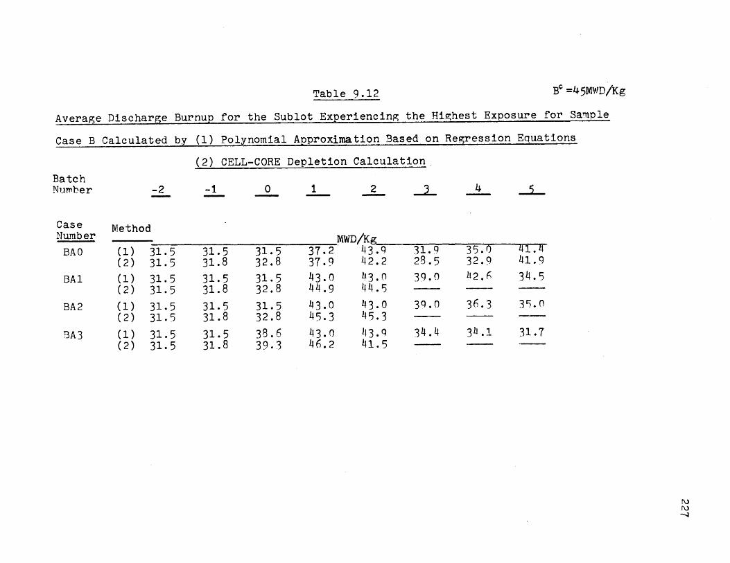
B4 =45MWD/Kg
Average Discharge Burnup for the Sublot Experiencing the Hiihest Exposure for Sample
Case B Calculated by (1) Polynomial Approximation Based on Regression Equations
(2) CELL-CORE Depletion Calculation
-2 -1 0 1
Method
(1) 31.5(2) 31.5
(1) 31.5(2) 31.5
(1) 31.5(2) 31.5
(1) 31.5(2) 31.5
31.531.831.531.831.531.831.531.8
31.532.831.532.831.532.838.639.3
37.237.943.044.943.045.3
2
MWD/Kg43.942.2
43.044.5
113.41.5
4
31.Q - 35.031.9 35.028.5 32.9
39.0 12.6
39.0
34.4
36.3
3)h.1
BatchNumber
CaseNumber
BAO
BAl
BA2
BA 3
_5-
41.441.934.5
35.0
31.7
Table 9.12

Table 9.13 B0 =50MWD/KgReload Enrichments. Batch Fractions, Cycle Energies and Revenue Requirements for the
Various Lowest Cost Cases Using the Method of Polynomial Approximation Sample Case B
CycleE(w/o) 1 2 3 _4 5fE (GWHt)
Target25450.Energy
TKO~-4fE
BB1 efE
BB2 6fE
BB3 6fE
BB4 efE
BB5 *fE
30730.33325510.
3.740.33325510.
4.550.29325340.
3.740.33325510.40550.29325340.
4.550.29325340.
4.570.29325450.
fE
30440. 21850. 19340. 20880.
4.360.33330470.4.360.33330470.
30790.33330310.4.360.33330470.
3.790.33330310.30790.33330310.3.260.37330440.
2.400.33322170.
2.700.29321270.
2.910.29321790.2.700.29321270.
2.910.29321790.
3.720.25321790.
4.310.25321850.
2.760.33320280.
30880.25319180.
30870.25319480.
3.100.29319260.
30090.29319320.
3.450.33317220.2.270.29317930.20610.29320020.
2.370.33317480.
2.710.33319930.
2.93 2.930.253 0.29319130.20110.2.83 3.260.253 0.29319340. 20880.
Revenue RequirementFor Actual Energy Corrected for Target
EnergyPo ly-nomial CELL-Appro-ximation.
COCO
(89.36 89.37
(
88.66 88.71
89.35 89.38
88.61 88.67
89.32 89.38
89.31 89.27
89.94 89.82
Po ly-nomial CELL-Appro- COCO
6 ximation
Difference)
89.92-0.01)
89.67(-0.05)
89.67(-0.04)
89.71(-0.05)
89.71(-0.05)
89.72(+0.04)
89.94(+0.12)
89.93
89.72
89.71
89.76
89.76
89.68
89.82
Case
B*
(ZO
11111191111 PIP PIN
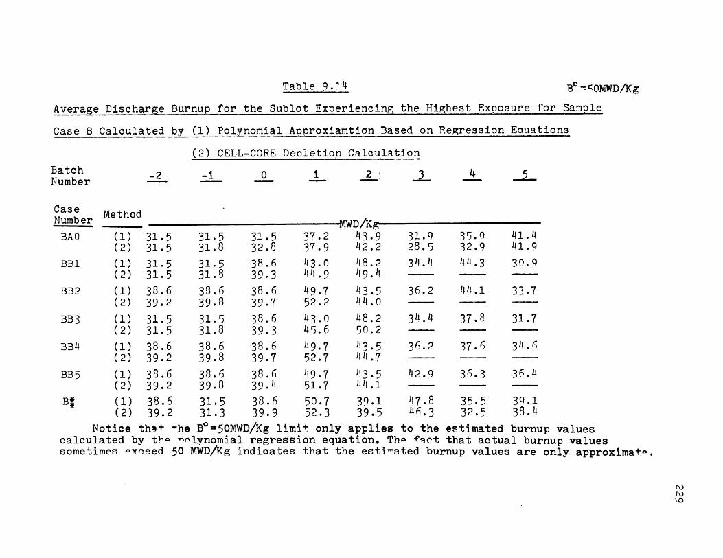
B. -COMWD/Kg
Average Discharge Burnup for the Sublot Experiencing the Highest Exposure for Sample
Case B Calculated by (1) Polynomial Approxiamtion Based on Regression Eauations
(2) CELL-CORE Depletion Calculation
31.531.531.531.5
(1) 38.6(2) 39.2
(1) 31.5(2) 31.5
38.639.238.639.238.639.2
-1
31.531.831.531.838.639.831.531.838.639.838.639.831.531.3
142.9 36.3
Notice that +he B*=50MWD/Kg limit only applies to the estimated burnup valuescalculated by t nnlynomial regression equation. The +qet that actual burnup valuessometimes Pxceed 50 MWD/Kg indicates that the esti.'ated burnup values are only approximato,
-2. 0
Method
1
(1)(2)
(1)(2)
BatchNumber
CaseNumber
BAO
BB1
BB2
BB3
BB4
BB 5
4
35.032.944.3
44.1
31.928.5314. 1
36.2
311.4
2 :
-MWD/Kg-43.942.2
43.5414.048.250.243.544.743.5414.139.139.5
31.532.838.639.338.639.738.639.338.639.738.639.438.639.9
37.237.943.044.949.752.2
43.045.649.752.749.751.7
50.752.3
(1)(2)
(1)(2)
(1)(2)
41 .41.930.9
33.7
31.7
3h.6
47.846.3
35.532.5
39.138.4
Table 9 .14

230
Case BI is the optimal solution arrived at by Dynamic Pro-
gramming. BI is more expensive than BAl by $0.17 million
dollars. However, the total savings of BI from the base
line BAO is only $0.11 million dollars. This is in great
contrast with the $2.5 million dollars saving reported by
Kearney. The difference is probably due to the different
methods of calculating TC.
Finally, it is important to notice that in the vicinity
of "the optimal solution", there are many sub-optimal solu-r
tions with roughly the same total cost. Some of these
solutions may have higher engineering margins in terms of
discharge burnup, power peaking and shut-down reactivity.
Hence,,the final choice should be based on these consider-
ations as well.
9.7 Estimates of Burnup Penalty w
The concept of burnup penalty wwas introduced in Chap-
ter 6,and it is defined for the non-steady state case by
Equation (7.10) in Chapter 7. For each cycle, there would be
a separate value for burnup penalty wc, which can be inter-
preted as the additional cost that would be incurred if the
burnup limitation on Cycle c were decreased by one unit.
Since the actual optimization algorithm solves by ex-
haustive search instead of by Equations (7.10) and (7.11),
burnup penalty is not calculated explicitly. However, the
order of magnitude of wrc can be infered by inspecting
Tables 9.7, 9.8, 9.9, and 9.10.
Tables 9.8 and 9.10 show that the discharge burnup is

231
well within the limit for almost all of the batches except
one in all cases. In other words, a single batch in each
case controls the values of the batch fractions. Hence,
by definition, the burnup penalties for those cycles not on
the border of the burnup constraints have the value zero.
The burnup penalty for the controlling batch can be
estimated by
c AB"c
where TU(E,*) is the optimal solution for and AO
and TU(Et**) is the optimal solution for Es and A*+ABOC
For sample case A, 'r2 for the second fuel batch is given by
the difference in TR between case AAl and AB1 divided by
the increment in B.
2 5(872/86.98)0106$ - 0.4 = 0.008-10 6 $/(MWD/Kg)2= 5(MWD/Kg) 5
This value of w is much smaller than that given in
Figure 6.7 for the steady state case. Similar results are
obtained for sample case B. Hence there is very little
incentive to increase the maximum allowable burnup limit
above the 45 MWD/Kg level.
9.8 Incremental Cost
Incremental cost of energy is defined as the additional
cost that would be incurred if an additional unit of energy
is produced in an optional fashion. In other words, if the reactor

232
is optimized for one set of cycle energy ES4.s -.- -. S 40.
TC(E ,f*) =minimum of TC(E ,f) with respect to f
and B0 <B (s P)and for the second set of cycle energies, ES +AEc the
reactor is reoptimized.
T6(Es +AE ,ft) = mininum of TC(Es +AEc,C C
with respect to f
and B>B (Es +AE , ft)then the incremenial costcof energy from the c-cycle
is given by
Tgs+AE ,t)-T(E ,f*)Ac'2 cE (9.5)
c
The values of TO are obtained from the regression equations.
In principle, one can use the. actual TO calculated from
CELL-COCO; However, for the purpose of this calculation, the
additional efforts involved in doing all the depletion analysis
are not justified. Tables 9.15, 16 show the values of fd($s
and Tf(I*+AEc,Pt) for various AEc for sample case A. Also
shown are the various f* and f . For many cases, f are
seen to be the same as ft For these cases, more or less
energy can be generated using the same combination of f*
However, for those cases that ft are not equal to f*
either the f* are not the least costly combination at the
new set of E +AE , or the f* are not feasible in
terms of discharge burnup. For AE c> 0 , feasibility con-
siderations change the ?* to ?t ; on the other hand,
for AE c< 0 , economics considerations cause the change.
Tables 9.15, .16 also show the incremental cost for various cycles
as a function of energy. In general, the incremental cost

Table 9.15
Calculation of Incremental Cost of Energy
Using Regression Equations. Sample Case A
Burnup Limit B = 45MWD/Kg
Batch Fraction for Cycle
1 2 3 14
BaseCase 0.293 0.293 0.293 0.293 0.333AAl
Positive Energy ChangeE=1000GWHtin Cycle
Revenue Incre-Requirement mental
5 Costmills/--10 $- KWHe
87.01872
1 0.333 0.293 0.293
2 0.293 0.293 0.293
3 0.293 0.293 0.293
4 0.293 0.293 0.293
5 0.293 0.293 0.293
Negative Energy ChangeAE=-1000GWHtin Cycle
1 0.293 0.293 0.293
2 0.293 0.253 0.253
3 0.293 0.293 0.293
4 0.293 0.293 0.293
5 0.293 0.293 0.293
0.293 0.333 87.5284
0.293 0.333 87.4265
0.293 0.333 87.3890
0.293 0.333 87.3170
0.293 0.333 87.2957
0.293 0.333 86.5642
0.253 0.293 86.5848
0.293 0.333 86.6605
0.293 0.333 86.7226
0.293 0.333 86.7443
1.56
1.22
1.15
0.91
0.845
1.395
1.33
1.095
0.905
o.84
233

234
Table 9.16
Calculation of Incremental Cost of Energy
Using Regression Equations. Sample Case A
Burnup Limit BO= 50MWD/Kg
Batch Fraction for Cycle Revenue Incre-Require- mental
1 2 3 4 5 ment CostMills/
--40 $- KWH
BaseCase 0.293 0.253 0.253AB1
Positive Energy ChangeAE01000GWHtin Cycle
1 0.293 0.253 0.253
2 0.293 0.293 0.293
3 0.293 0.253 0.293
4 0.293 0.253 0.253
5 0.293 0.253 0.253
Negative Energy ChangeAE=-1000GWHtin Cycle
1 0.293 0.253 0.253
2 0.293 0.253 0.253
3 0.293 0.253 - 0.253
4 0.293 0.253 0.253
5 0.293 0.253 0.253
0.253 0.293 86.9890
0.253 0.293 87.4642
0.293 0.333 87.4265
0.293 0.293 87.3848
0.253 0.293 87.3047
0.253 0.293 87.2748
0.253
0.253
0.253
0.253
0.253
0.293
0.293
0.293
0.293
0.293
86.5345
86.5848
86.5860
86.6761
86.7064
1.46
1.335
1.21
0.965
0.875
1.395
1.24
1.24
0.955
0.865

235
increases as more energy is produced. However, for those
cases in which ?*# 1 , incremental cost would have a
negative slope. In the limit that AEc 0 X c would
approach infinity for those cases that i* . This
is mainly due to the fact that in the present model one can
only change batch fraction by a discrete amount, and the
objective functions of the two discrete combinations of
and Pt have a finite difference. If batch fractions
could be varied in a continuous fashion, these singularities
would not be present and the incremental cost would vary
continuously in a pattern similar to Figure 6.8.
Table 9.1V and Table 9.18 show values of the objective
function and the incremental costs for various AEc for
sample case B. The same phenomenon of negative sloping
incremental cost is observed.
9.9 Summary and Conclusions
Using cycle energies P and batch fractions I as
independent variables, a set of regression equations based on
polynomials in these independent variables hasbeen obtained.
These predict the objective function to an accuracy of within
+ 0.1% and average discharge burnup to an accuracy of within
+10%. An optimization algorithm based on the principle of ex-
haustive search is developed. For every specified set of cycle
energies, this algorithm results in five or more sub-optimal
cases that bracket the optimal solution. These cases can be
analysed further by more elaborate depletion codes.
The results of the regression analysis and the optimiza-
tion procedures indicate that the objective function for

Table 9.17
Calculation of Incremental Cost of Energy
Using Regression Equations. Sample Case B
Burnup Limit B = 45MWD/Kg
Batch Fraction for Cycle
1 2 3
0.333 0.373 0.293
4 5
RevenueRequirement
Incre-mentalCost
Mills/KWHe
0.253 0.293 89.8251
Positive Energy ChangeAE=1000GWHtin Cycle
1 0.333 0.373 0.293
2 0.333 0.373 0.293
3 0.333 0.373 0.293
4 0.333 0.373 0.293
5 0.333 0.373 0.293
Negative Energy ChangeAE=-1000GWHtin Cycle
1 0.333 0.373 0.293
2 0.333 0.373 0.293
3 0.333 0.373 0.293
4 0.333 0.373 0.293
5 0.333 0.373 0.293
0.253 0.293 90.2916
0.253 0.293 90.2424
0.253 0.293 90.1845
0.293 0.333 90.1255
0.263 0.293 90.1049
0.253 0.293 89.3766
0.253 0.293 89.4070
0.253 0.293 89.4773
0.253 0.293 89.5224
0.253 0.293 89.5484
Bas eCaseBAl
1.435
1.28
1.10
0.91
0.915
1.375
1.28
1.07
0.925
0.85
236

Table 9.18
Calculation of Incremental Cost of Energy
Using Regression Equations. Sample Case B
Burnup Limit B = 50MWD/Kg
Batch Fraction for Cycle
4
Revenue
5
Incre-Requirement mental
-10 $-
Cost
in Mills/
BaseCaseBBL1
0.333 0.333 0.293
Positive Energy ChangeAE=1000GWHtin Cycle
1 0.333 0.333 0.293
2 0.293 0.333 0.293
3 0.333 0.333 0.293
4 0.333 0.333 0.293
5 0.333 0.333 0.293
Negative Energy ChangeAE=-1000GWHtin Cycle
1 0.293 0.333 0.293
2 0.293 0.293 0.253
3 0.333 0.333 0.253
4 0.333 0.333 0.293
5 0.333 0.333 0.293
0.253 0.293 89.6715
0.253 0.293 90.1380
0.253 0.293 90.0775
0.253 0.293 90.0309
0.253 0.293 89.9772
0.253 0.293 89.9513
0.253 0.293 89.1628
0.253 0.293 89.1515
0.253 0.293 89.3229
0.253 0.293 89.3687
0.253 0.293 89.3947
237
1 2 3
1.435
1.10
0.93
0.86
1.56
1.60
1.07
0.845

238
cas-es A and B is insensitive to batch fraction changes, if
the same cycle energies are produced. Hence, engineering
considerations should be the principal criteria in the
selection process for those problems. Since batch fraction
cannot be varied continuously, incremental cost of energy
varies in a series of discrete jumps. This problem would
have been less severe if the increments in batch fraction
had been made smaller.

239
CHAPTER 10.0
CONCLUSIONS AND RECOMMENDATIONS
10.1 Conclusions
The following conclusions are obtained from this
thesis research.
(1) The Inventory Value Method for evaluating worth
of nuclear fuel inventories to be used in
calculating finite planning horizon revenue
requirement is adequate for the purpose of
scheduling energy and nuclear in-core
optimization.
(2) Three methods are proposed for calculating
incremental cost of energy for the fixed batch
fraction case. The Linearization Method
and the Inventory Value method for calculating
incremental cost -of energy are both suitable
for the initial stages of optimal energy
scheduling. The Rigorous Method is very time
consuming and expensive and should be used only
in the final stages of optimal energy scheduling.
(3) For the problem of nuclear in-core optimization
under steady state conditions with variable
batch fractions and reload enrichments, the
optimal solution is practically always on the
boundary of the burnup constraints. Hence,
there are strong incentives to increase the
burnup limits.

240
(4) For the problem of nuclear in-core optimization
under non-steady state conditions, the Method
of Piece-Wise Linear Approximation is applicable
for the cases where there are large variations
of objective function near the optimal solution.
It is not applicable for economic situations where
there is a broad region of optimality.
(5) The Method of Polynomial Approximation gives
accurate values of the optimal solutions, even
though the objective function is very flat
near the optimum.
(6) Since the objective function is insensitive to
large variations in batch fractions, selection of
the optimal solution can be based primarily on
other considerations, such as engineering margins.
10.2 Recommendations
The depletion code CELL-CORE should be modified in
order that the batch fraction can be varied continuously.
This modification would enable the efficient usage of the
Method of Linear Approximation instead of Piece-Wise Linear
Approximation or Polynomial Approximation. Once the optimal
batch fraction in the continuum is located, the realistic
batch fraction to be used in refuelling would be given by
the number of integral fuel assemblies which is closest
to the continuum optimal solution.

Finally, the algorithm of optimal energy schedule
should be modified so that the polynomial equations from
regression analysis could be used directly, instead of the
present indirect usage which require intermediate calculations
of incremental cost. It is recommended that a quadratic
programming algorithm, or an even higher order programming
algorithm should be used in the optimal energy scheduling
procedures, so that the higher order derivatives can be
used directly.
241

242
Biographical Note
Hing Yan Watt was born in Kowloon, Hong Kong on
March 4, 1948. He received his elementary and secondary
education on this island city, and was graduated from
St. Paul's College in June 1966.
In September 1966, he enrolled at Massachusetts Institute
of Technology where he studied in the Department of Civil
Engineering. He was elected to membership in Chi Epsilon
engineering honorary society in 1968. He received his
Bachelor of Science degree in Civil Engineering in June 1969.
In September 1969, he entered the Department of Nuclear
Engineering at M.I.T. and was granted the degree of Master of
Science in August 1970.
Mr. Watt is married to the former An-Wen Cheng of
Shanghai, China.

Brief Description of the
Code Name
MOVESCIV
Time of
Time ofDevelopment
Early 1971
Appendix A
Several Versions of CORE
Description ofRefuelling Options
N-zone modifiedscatter refuelling(Batch fractioncannot be changedin adjacent cycles)
Homogenizationof Fuel Batches
Fuel propertieshomogenized onlyonce when they arescattered from theouter annulus intothe inner region.
EconomicsCalculations
January 1972
April 1972
November 1972
(same as MOVESCIV except it is much faster)
Non-integral batchfraction. Variablebatch fraction inadjacent cycles
Fuel properties inthe inner region arehomogenized at thebeginning of everycycle
(same as CORE(April 1972)) Fuel cycleca)culationson per batchbasis. Endinginventorycalculated byInventoryValue Method
COPE
CORE
Coco

244
Appendix B
Econonips and FuelCycle Cost Parameterq
Fuel Cycle Financi.ng
Investor-owned utility
Fraction of bond financing 0.55
Fraction of preferred stock 0.10
Fraction of common stock 0.35
Rate of return on bonds, fraction per year 0.08
Rate of return on preferred stock, fraction
per year 0.08
Rate of return on common stock, fraction
per year 0.13
Tax rate 0.50
Government-owned utility
Fraction of bond financing 1.00
Rate of return on bonds, fraction per year 0.0755
Lead Times: Time of transaction prior to the
beginning of irradiation , in days
Purchase of uranium concentrate 127
Conversion of U3 08 to UF6 127
Enrichment 97
Plutonium purchase 97
Fabrication 40

Lag Times: Time of transactions after the end of the
irradiation, in days
Shipping 182
Reprocessing 212
Conversion of UNH to UF 6 212
Credit for reprocessed fuel 212
Lag time for receipt of revenue:
60 days after the mid-point of the generation period;
one single payment
Charges for materials and services
Price of U 3 0 8 , $/ib 8.00
Conversion of U3 08 to UF 6, $/kg U 2.20
Enrichment $/kg SWU 32.00
Enrichment plant tails composition, w/o U-235 0.25
Fabrication, $/kg U 70.00
Shipping, $/kg initial fuel metal 4.00
Reprocessing, $/kg initial fuel metal 30.57
Conversion of UNH to UF6, $/kg U 5.60
Process Yields
Fabrication 0.99
Reprocessing 0.99
Conversion of U 308 to UF6 0.995
Conversion of UNH to UF6 0.995
#Consistent with a natural UF 6 price of $23.46/kg U

246
Appendix CNOMENCLATURE
TO Revenue requirement
TCA
TCB
TCs
-NTCC
TU1
TC
TU
Revenue
Revenue
Revenue
Revenue
Revenuenuclide
Revenueservice
Revenue
Revenuenuclide
Revenueservice
Revenue
Revenue
R Revenue requirement for a batch
R Revenue requirement for Reactor A Batch b
R Revenue requirement for Reactor B Batch bb
Z. Component i of the various fuel cycle expenses,$
Z Nuclide component of the fuel cycle expense1
Z Service component of the fuel cycle expense1
ZU Cost of U feed as UF6ZUCredit for U discharge as UF6
ZF Fuel fabrication cost
requirement
requirement
requirement
requirement
requirementcomponent
requirementcomponent
requirement
requirementcomponent
requirementcomponent
requirement
requirement
for Reactor A
for Reactor B
for nuclear sub-system
for the indefinite horizon
for the indefinite horizon
for the indefinite horizon
for planning horizon I
for planning horizon I
for planning horizon I
up to and including Cycle 1
for reactor r in the planning horizon

247
Zg . Shipping cost
Z Reprocessing cost
ZC Conversion cost
Z Pu Plutonium credit
V Value of nuclear fue]
Vi Value of nuclear fuel at the begininitialhorizon I
VfIna Value of nuclear fuel at the endohorizon I
V Value of nuclear fuel at hte end ohorizon I
Vb(t1 1.) Value of nuclear fuel batch b at t
X t Incremental cost of energy
A rc Incremental cost of energy for react
Ac Incremental cost of energy for cycle
7 Burnup penalty
Tc Burnup penalty for cycle c
7b Burnup penalty for batch b
p Negative of burnup penalty (-n)
Sc Enrichment for cycle c w/o U-235
fc Batch fraction for cycle c
B Average discharge burnup
Bc Average discharge burnup for cycle c
Bb Average discharge burnup for batch b
BO Maximium allowable burnup limit
ning of planning
f planning
f planning
ime ti,
or r cycle c
c
Initial state of the reactor at the beginning oftime horizon
Corporate income tax rate
Effective cost of money, per year
?1
T
x

248
t Time
tb Time when batch b is charged to the reactor
ti Time when fuel cycle expense i is paid
tc Time when cycle c begins
t Time when fuel cycle expense j in time horizon I is naid
tj, Time when planning horizon I begins
tI,, Time when planning horizon I ends
Coefficient matrix of derivative of energy with respect
to enrichment
a Derivative of revenue requirement with respect toenrichment of Cycle c
Derivative of revenue requirement with respect toc batch fraction of Cycle c
ykc Derivative of energy for Cycle k with respect toenrichment of Cycle c
6 Derivative of energy for Cycle k with resnect tokc batch fraction of Cycle c
(kc Derivative of discharge burnuo of Cycle k with respectto enrichment of Cycle c
kc Derivative of discharge burnuo of Cycle k with respectto batch fraction of Cycle c
E(nb )Burnup coefficient for a batch of fuel that has beenirradiated for nb cycles
a c Multiple regression coefficient
cMultiple regression coefficient
ye Multiple regression coefficient
c Multiple regression coefficient
Superscripts
*t Denote optimal values

249
Superscripts
+ Coefficients evaluated at positive values
- Coefficients evaluated at negative values

250
Appendix DList of References
(AEP1) American Electric Power Corporation.
Personal communication with Nicholas Tibberts. Nov.1972
(Bl) J.J. Beaudreau, "Development and Evaluation of the
Point Depletion Code CELL", S.M. Thesis
Nuclear Engineering Department. M.I.T. June 1967
(B2) Manson Benedict, "Economics of Nuclear Power."
Class notes, Nuclear Engineering Department. M.I.T.1972
(CEl) Commonwealth Edison, Personal communication with
Edward Koncel 1971
(CE2) Commonwealth Edison, Personal communication with
John Bukovski 1971
(CJl) James Conklin, "MITCOST, a Levelized Fuel Cycle Cost
Code" Nuclear Engineering Department Code Library.
July 1971
(Dl) Paul F. Deaton, "A System Integration and Optimization
Model for Nuclear Power Management," Ph.D. Thesis,
Nuclear Engineering Department. M.I.T. 1973.
(DZl) George Dantzig, LINEAR PROGRAMMING AND EXTENSIONS,
Princeton University, Press, Princeton, N.J. 1963
(Gl) E.L. Grant and W.G. Ireson, PRINCIPLES OF ENGINEERING
ECONOMY, Ronald Press Co. New York, 1970, pp. 496-505,
509-511.
(Kl) Joseph P. Kearney, "Simulation and Optimization
Techniques for Nuclear In-Core Fuel Management
Decisions." Ph.D. Thesis, Nuclear Engineering
Department, M.I.T. 1972
251
(K2) L.K. Kirchmeyer, "Economic Operation of Power Systems."
John Wiley and Sons. pp.4 0 1958
(R1) Terrance Rieck, Research in Progress. Nuclear
Engineering Department. M.I.T. 1972
(So) "San Onofre Nuclear Generating Station Reference Core
Design" WCAP-3269-7 (1965)
(W1) Hing Yan Watt, MITCOSTI, computer code developed at
M.I.T. 1972. Available from Nuclear Engineering
Department. M.I.T.
(W2) Hans Widmer, "The Optimal Utilization of a Nuclear
Power Plant with Fixed Fuelling Schedule" Ph.D. Thesis
Nuclear Engineering Department. M.I.T. 1970
(Z1) Zion Station, Units 1 and 2, Final Safety Analysis
Report, Commonwealth Edison Company, Chicago, Illinois.