of - beta analytic: biobased content testing services - astm … · 2010-06-18 · '4c...
TRANSCRIPT

[RADIOCARBON, VOL 32, No. 1, 1990, P 37-58]
THE USE OF RADIOCARBON MEASUREMENTS IN ATMOSPHERIC STUDIES1
M R MANNING, D C LOWE, W H MELHUISH, R J SPARKS, GAVIN WALLACE, C A M BRENNINKMEIJER and R C McGILL
Institute of Nuclear Sciences, Department of Scientific and Industrial Research Lower Hutt, New Zealand
ABSTRACT. '4C measured in trace gases in clean air helps to determine the sources of such gases, their long-range transport in the atmosphere, and their exchange with other carbon cycle reservoirs. In order to separate sources, transport and exchange, it is necessary to interpret measurements using models of these processes. We present atmospheric ' 4C02 measurements made in New Zealand since 1954 and at various Pacific Ocean sites for shorter periods. We analyze these for latitudinal and seasonal variation, the latter being consistent with a seasonally varying exchange rate between the stratosphere and troposphere. The observed seasonal cycle does not agree with that predicted by a zonally averaged global circulation model. We discuss recent accelerator mass spectrometry measurements of atmospheric 14CH4 and the problems involved in determining the fossil fuel methane source. Current data imply a fossil carbon contribution of ca 25%, and the major sources of uncertainty in this number are the uncertainty in the nuclear power source of 14CH4, and in the measured value for S'4C in atmospheric methane.
INTRODUCTION
Trace gases in the atmosphere play a crucial role in determining our environment. Greenhouse gases in the troposphere determine the earth's temperature through selective absorption of infra-red radiation. Ozone in the stratosphere filters out ultra-violet radiation that would destroy complex organic molecules essential for life. Because the amounts of these gases are small and the balance of processes maintaining them complex, they are a potentially fragile part of our environment.
Many of the trace gases that must be studied in relation to changes in climate and atmospheric chemistry contain carbon. For these gases, isotopic measurements are directly relevant in determining sources and sinks, because sources will have different isotopic composition and sinks will involve fractionation. The importance of carbon isotope measure- ments in building global budgets for gases such as CO2 (Keeling, Mook & Tans 1979; Peng et al 1983), CH4 (Ehhalt 1973) and CO (Stevens et al 1972) has been recognized for some time.
The atmospheric concentration of gases with lifetimes of the order of minutes or less is
determined by local atmospheric chemistry and the presence or absence of light. For gases with lifetimes of many years, concentrations are relatively homogeneous due to atmospheric mixing. Between these extremes there are atmospheric species with intermediate lifetimes, the concentration of which depends on both atmospheric transport and the distribution of sources and sinks. To understand the varying concentrations of such species, we must combine quantitative information on advection and diffusion in the atmosphere with information on the spatial distribution of sources and sinks. This is a difficult task, but holds the prospect that we may determine a consistent picture of all the processes involved.
Each of the gases C02, CH4 and CO is a candidate for study using a detailed physical and chemical model of the atmosphere. Extensive modeling of the annual cycle of CO2 concentrations (Trabalka 1985; Heimann & Keeling 1986) has shown that even though this gas has a lifetime in the atmosphere of many years, the latitudinal and seasonal variation of its concentration yields information on long-range atmospheric transport.
CH4 has a lifetime similar to that of C02, but is a complementary tracer of atmospheric transport because the distribution of its sinks is quite different. While the sinks for CO2 are all at the surface, the dominant sink of CH4 is through reaction with the OH radical distributed throughout the atmosphere. The OH radical is produced photolytically in the troposphere and its maximum diurnal concentration, and therefore the sink strength for CH4, varies considerably with latitude, altitude and season (Logan et al 1981).
Reaction with the OH radical is also the major sink for CO (Volz, Ehhalt & Derwent 1981), so CO has a sink structure similar to CH4. As the lifetime of CO months) is
shorter than the time required to mix throughout the troposphere, this gas does not become
This paper was presented at the 13th International Radiocarbon Conference, June 20-25, 1988 in Dubrovnik, Yugoslavia.
37

38 M R Manning et al
fully dispersed from its sources. In regions where the mean transit time for CO arrival from a source is of the order of its lifetime, we can expect significant variation in concentrations as a result of transient changes in atmospheric transport.
The natural cosmogenic formation of 14C in the stratosphere (Lal & Peters 1962) leads to both 1400 and 14002. As this 14C production is greatest in the stratosphere, we expect a natural vertical gradient in atmospheric 14C. Human intervention through nuclear weapons testing, which put 14C in the stratosphere, and release of fossil carbon from the surface has enhanced this natural gradient. Relatively rapid mixing in the troposphere can be expected to dissipate this gradient at lower altitudes, but across the tropopause and in the strato- sphere it will persist.
Thus, 14C is a useful tracer of transport in the atmosphere, and particularly of vertical transport. The longer-lived species such as 14C02 and 1 CH4 provide information on the longer time scales associated with stratosphere to troposphere and interhemispheric ex- change, whereas 14C0 can provide information on the shorter time-scale movements associated with transport within a hemisphere.
We show here that the seasonal component of a 32-yr atmospheric 14C02 record can be used to infer stratospheric residence times for CO2. Our data are compared with a two-dimensional model of atmospheric transport and discrepancies are shown which imply either deficiencies in present modeling of vertical transport, or thelpresence of complex sources and sinks of C or both. We also show how measurements of CH4 can identify the relative strengths of fossil and modern sources of methane, and can set limits on the production of this species from nuclear power plants.
MEASUREMENTS OF ATMOSPHERIC 14CO9 IN THE SOUTH PACIFIC
Measurements of 14C in atmospheric CO2 at Wellington, New Zealand and at other South Pacific sites ranging from the Antarctic to the Equator, were initiated by T A Rafter and G J Fergusson in the early 1950s. Early results and procedures are reported elsewhere (Rafter 1955; Rafter & Fergusson 1959; Rafter & O'Brien 1970). Our data report the results of this program up to May 1987.
The sampling procedures used to obtain nearly all the data are described by Rafter and Fergusson (1959). Trays containing ca 2L of 5 normal NaOH carbonate-free solution are exposed for intervals of 1-2 weeks, and the atmospheric CO2 absorbed during that time is recovered by acid evolution. Considerable fractionation occurs during absorption into the NaOH solution, and the standard fractionation correction (Stuiver & Polach 1977) is used to determine a Q14C value corrected to S13C = - 25°/.
A few early measurements were made by bubbling air through columns of NaOH for several hours. These samples can be readily identified in the data as their 313C value is much higher (ie, closer to the ambient air value). Also, some samples reported here were taken using BaOH solution or with extended tray exposure times. These variations in procedures do not appear to affect the results.
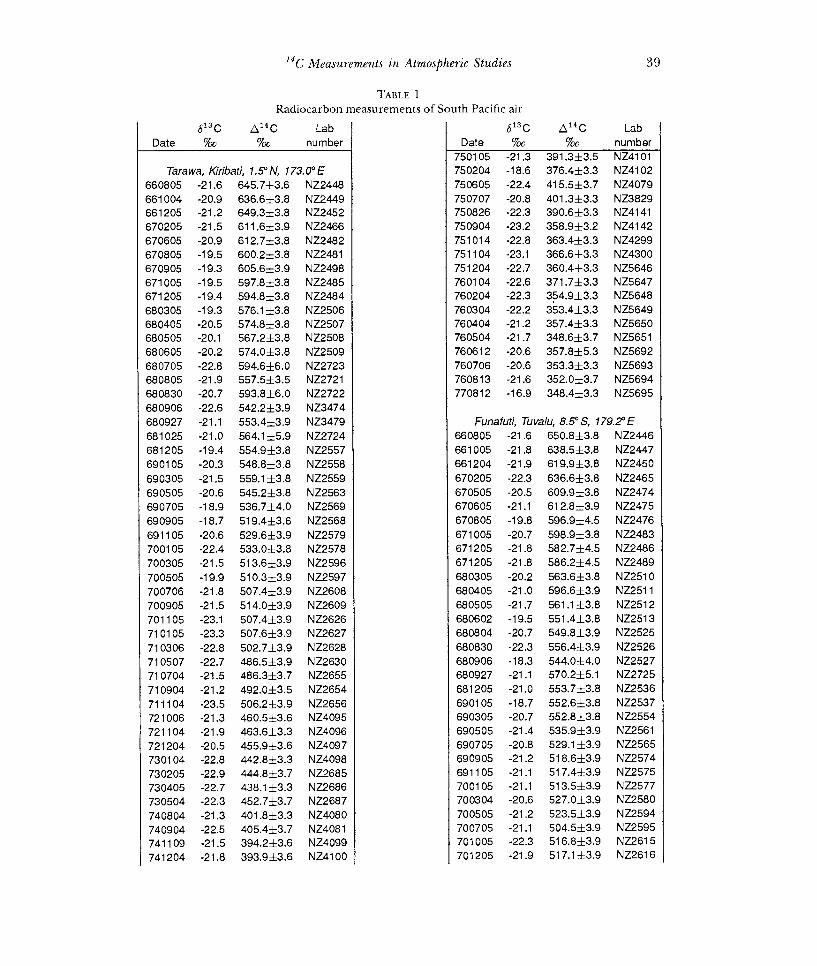
Table 1 lists the Wellington data for the period, Dec 1954-May 1987, and data for shorter periods at six other sites. Dates refer to the mid-point of the sampling interval, and an asterisk denotes a sample for which contamination is known or suspected. Figures 1A, B show the data after discarding these suspect cases.
Low latitudinal gradients are to be expected in the South Pacific, as the sources of 14002 are far from the sampling sites and CO2 has a mean lifetime in the atmosphere which is long compared to the time required for tropospheric mixing. This is borne out by our data which show only small variations between sites. Quantifying these differences is made difficult by the noise level, which appears to exceed the error due to counting statistics, and by the sparsity of data from different sites for common times.
Table 2 summarizes the station differences relative to the Wellington station, using months where data are common to both. This suggests that 14C levels in atmospheric CO2 were slightly higher in the Equatorial Pacific than at mid-southern latitudes, and were
14C Measurements in Atmospheric Studies 39
TABLE 1
Radiocarbon measurements of South Pacific air 613 C A14C Lab
Date %o %o
750105 -21.3 391.3±3.5 Tarawa, Kiribati, 1.5° N, 173.0° E 750204 -18.6
660805 -21.6 645.7±3.6 661004 -20.9 636.6±3.8 661205 -21.2 649.3±3.8 670205 -21.5 611.6±3.9 670605 -20.9 612.7±3.8 670805 -19.5 600.2±3.8 670905 -19.3 605.6±3.9 671005 -19.5 597.8±3.8 671205 -19.4 594.8±3.8 680305 -19.3 576.1±3.8 680405 -20.5 574.8±3.8 680505 -20.1 567.2±3.8 680605 -20.2 574.0±3.8 680705 -22.8 594.6±6.0 680805 -21.9 557.5±3.5 680830 -20.7 593.8±6.0 680906 -22.6 542.2±3.9 680927 -21.1 553.4±3.9 Tuvalu, 8.5° S, 179.2° E 681025 -21.0 564.1±5.9 681205 -19.4 554.9±3.8 690105 -20.3 548.8±3.8 690305 -21.5 559.1±3.8 690505 -20.6 545.2±3.8 690705 -18.9 536.7±4.0 690905 -18.7 519.4±3.6 691105 -20.6 529.6±3.9 700105 -22.4 533.0±3.8 700305 -21.5 513.6±3.9 700505 -19.9 510.3±3.9 700706 -21.8 507.4±3.9 700905 -21.5 514.0±3.9 701105 -23.1 507.4±3.9 710105 -23.3 507.6±3.9 710306 -22.8 502.7±3.9 710507 -22.7 486.5±3.9 710704 -21.5 486.3±3.7 710904 -21.2 492.0±3.5 711104 -23.5 506.2±3.9 721006 -21.3 460.5±3.6 721104 -21.9 463.6±3.3 721204 -20.5 455.9±3.6 730104 -22.8 442.8±3.3 730205 -22.9 444.8±3.7 730405 -22.7 438.1 ±3.3 730504 -22.3 452.7±3.7 740804 -21.3 401.8±3.3 740904 -22.5 405.4±3.7 741109 -21.5 394.2±3.6 741204 -21.8 393.9±3.6 NZ4100 701205 -21.9 517.1±3.9 NZ2616
40 M R Manning et al
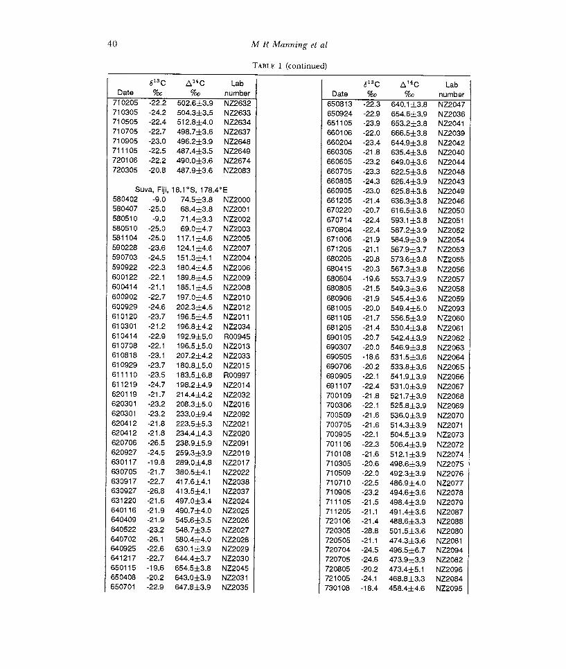
TABLE 1 (continued)
613 C Q14C Lab C Date %o %o
710205 -22.2 502.6±3.9 710305 -24.2 504.3±3.5 710505 -22.4 512.8±4.0 710705 -22.7 498.7±3.6 710905 -23.0 496.2±3.9 711105 -22.5 487.4±3.5 720106 -22.2 490.0±3.6 720305 -20.8 487.9±3.6
660805 -24.3 626.4±3.9 Suva, Fiji, 18.1 °S, 178.4°E 660905 -23.0
580402 -9.0 74.5±3.8 580407 -25.0 68.4±3.8 580510 -9.0 71.4±3.3 580510 -25.0 69.0±4.7 581104 -25.0 117.1±4.6 590228 -23.6 124.1±4.6 590703 -24.5 151.3±4.1 590922 -22.3 180.4±4.5 600122 -22.1 189.8±4.5 600414 -21.1 185.1±4.5 600902 -22.7 197.0±4.5 600929 -24.6 202.3±4.5 610120 -23.7 196.5±4.5 610301 -21.2 196.8±4.2 610414 -22.9 192.9±5.0 610708 -22.1 196.5±5.0 610818 -23.1 207.2±4.2 610929 -23.7 180.8±5.0 611110 -23.5 183.5±6.8 611219 -24.7 198.2±4.9 620119 -21.7 214.4±4.2 620301 -23.2 208.3±5.0 620301 -23.2 233.0±9.4 620412 -21.8 223.5±5.3 620412 -21.8 234.4±4.3 620706 -26.5 238.9±5.9 620927 -24.5 259.3±3.9 ±3.9 630117 -19.8 289.0±4.8 630705 -21.7 380.5±4.1 630917 -22.7 417.6±4.1 630927 -26.8 413.5±4.1 631220 -21.6 497.0±3.4 640116 -21.9 490.7±4.0 640409 -21.9 545.6±3.5 640522 -23.2 548.7±3.5 640702 -26.1 580.4±4.0 640925 -22.6 630.1±3.9 641217 -22.7 644.4±3.7 650115 -19.6 654.5±3.8 650408 -20.2 643.0±3.9 650701 -22.9 647.8±3.9 NZ2035 730108 -18.4 458.4±4.6 NZ2095

l4C Measurements in Atmospheric Studies 41
TABLE 1 (continued)
613C Q14G Lab
Date %o %o
730205 -21.1 451.3±3.7 730406 -20.4 444.6±3.3 730605 -23.0 433.6±3.3 730805 -23.9 456.2±3.7 731005 -23.9 423.1±3.3 731126 -22.5 430.7±7.4 731207 -21.3 456.5±3.3 740106 -20.9 427.3±3.7 740319 -22.4 409.8±3.7 740405 -21.6 415.2±3.7 740505 -21.4 416.1±4.4 ±3.9 740607 -21.4 403.8±3.7 750307 -21.6 392.6±3.3 750404 -21.8 384.1±3.3 ±3.9 750504 -19.7 379.0±3.3 750608 -22.0 389.3±3.7
681003 -19 8 9 515 9±3 Melbourne, Australla, 37.8°S, 144.9°E 681031
.
-22.8 . .
521.8±3.9 581104 -23.6 76.5±4.0 590229 -24.6 103.3±3.8 590703 -25.1 101.5±4.6 590926 -25.2 136.6±4.5 600122 -22.4 161.5±4.5 600415 -21.4 182.1±4.5 600708 -23.0 155.1±4.6 600930 -21.0 173.0±4.5 601112 -23.5 181.7±4.5 610120 -22.5 188.8±4.5 610929 -20.7 183.2±4.0 611219 -19.0 185.2±4.0 620413 -21.3 198.6±4.0 620928 -22.5 221.8±5.2 630118 -18.2 240.9±4.1 630705 -21.0 282.3±3.9 630926 -20.5 348.9±3.8 631219 -19.4 411.5±3.8 640116 -21.6 436.8±3.8 640410 -19.7 486.6±4.0 ±6.7
640702 -20.3 512.0±4.0 640925 -20.2 560.3±3.9 New Zealand, 41.3° S, 174.8° E
641218 -20.5 574.4±3.9 650115 -20.6 609.3±3.8 650409 -20.1 608.0±3.9 650520 -19.8 589.8±3.8 651001 -20.9 612.5±3.8 651105 -20.9 620.7±3.8 651205 -20.1 516.9±3.9 660107 -20.2 610.2±3.8 660305 -21.1 614.0±3.8 660505 -22.8 614.9±3.8 660605 -20.5 587.3±3.9 NZ2440 561021 -9.0 13.6±4.7 NZ2110
42 M R Manning et al
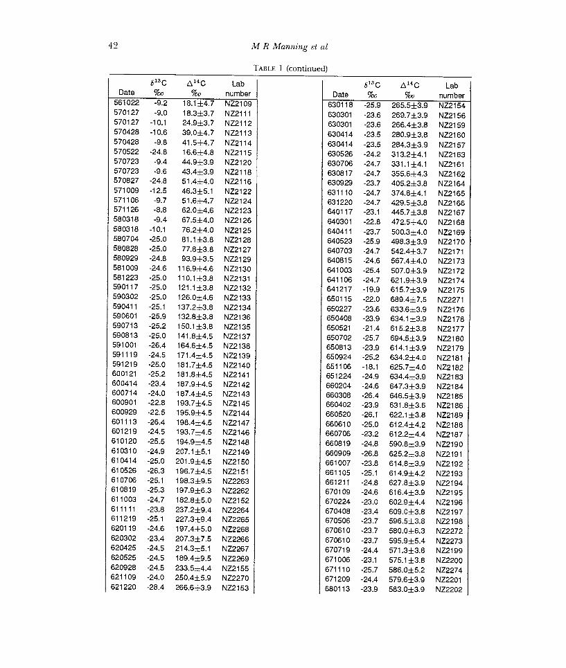
TABLE 1 (continued) 5130 &4C Lab
Date %o %o 561022 -9.2 18.1 ±4.7 570127 -9.0 18.3±3.7 570127 -10.1 24.9±3.7 570428 -10.6 39.0±4.7 570428 -9.8 41.5±4.7 570522 -24.8 16.6±4.8 570723 -9.4 44.9±3.9 570723 -9.6 434±3.9 570827 -24.8 51.4±4.0 571009 -12.5 46.3±5.1 571106 -9.7 51.6±4.7 571126 -8.8 62.0±4.6 580318 -9.4 67.5±4.0 580318 -10.1 76.2±4.0 580704 -25.0 81.1 ±3.8 580828 -25.0 77.8±3.8 580929 -24.8 93,9±3.5 581009 -24.6 116.9±4.6 581223 -25.0 110.1±3.8 590117 -25.0 121.1±3.8 590302 -25.0 126.0±4.6 590411 -25.1 137.2±3.8 590601 -25,9 132.8±3.8 590713 -25.2 150.1±3.8 590813 -25.0 141.8±4.5 591001 -26.4 164.6±4.5 591119 -24.5 171.4±4.5 591219 -25.0 181.7±4.5 600121 -25.2 181.8±4.5 600414 -23.4 187.9±4.5 600714 -24.0 187.4±4.5 600901 -22.8 193.7±4.5 600929 -22.5 195.9±4.5 601113 -26.4 198.4±4.5 601219 -24.5 193.7±4.5 610120 -25.5 194.9±4.5 610310 -24.9 207.1±5.1 610414 -25.0 201.9±4.5 610526 -26.3 196.7±4.5 610706 -25.1 198.3±9.5 610819 -25,3 197.9±6,3 611003 -24.7 182.8±5.0 611111 -23.8 237,2±9.4 611219 -25.1 227.3±9.4 620119 -24.6 197.4±5.0 620302 -23,4 207.3±7.5 620425 -24.5 214.3±5.1 620525 -24.5 189.4±9.5 620928 -24.5 233.5±4.4 621109 -24.0 250.4±5.9 621220 -28.4 266.6±3.9 NZ2153 680113 -23.9 583.0±3.9 NZ2202

14C Measurements in Atmospheric Studies 43
TABLE 1 (continued)
L 14C Lab Date %o %o
680211 -24.5 582.5±3.9 680311 -22.5 572.8±3.6 680406 -23.9 547.6±3.7 ±3.6 680531 -24.8 560.5±3.9 680607 -24.6 561.7±3.9 680705 -26.3 550.4±3.9 680809 -24.7 538.1 ±3.9 680830 -23.8 535.5±3.8 680906 -23.7 531.5±3.9 681004 -24.6 532.8±3.9 681018 -24.7 537.6±3.9 681102 -25.3 541.9±3.9 681108 -26.9 541.2±3.9 ±3.3 681206 -23.8 539.6±3.9 690110 -24.3 539.1 ±3.9 690207 -23.1 537.7±3.8 690308 -23.3 550.4±3.8 690413 -23.4 545.4±3.8 690502 -23.1 530.4±4.0 ±3.3 690509 -22.8 539.6±3.9 690607 -23.4 525.2±4.2 690711 -23.2 526.3±3.9 690809 -23.0 522.8±3.9 690905 -23.5 544.9±3.8 691010 -25.2 531.2±3.9 691103 -23.2 523.0±3.9 691205 -22.5 510.2±3.9 700109 -22.5 510.2±3.9 700306 -22.5 535.3±3.9 700410 -22.1 520.4±3.9 700509 -22.4 513.5±3.9 700606 -23.3 516,2±3.9 700710 -23.8 505.9±3.9 700807 -23.6 497.4±3.5 ±3.7 700911 -24.5 508.0±3.9 701010 -24.3 498.6±3.9 701106 -23.3 497.6±4.0 ±3.7 701223 -22.7 495.6±3.9 710110 -22.3 500.6±3.9 710205 -23.8 494.7±3.7 710305 -24.6 508.3±3.9 710409 -24.8 501.0±3.9 710507 -24.9 499.7±3.9 710611 -24.6 499.0±3.9 710709 -25.9 494.2±4.1 710808 -23.5 483.3±4.0 710910 -24.5 478.8±4.5 711010 -24.0 492.5±3.9 711203 -24.8 479.3±3.9 720109 -23.9 484.5±3.6 720206 -24.7 491.6±4.0 NZ2253 761011 -22.9 344.2±5.1 NZ5673
44 M R Manning et al
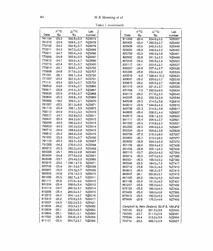
TABLE 1 (continued)
613C &4C Lab Date %o %
761104 -25.3 346.5±3.3 761210 -23.6 329.6±3.7 770103 -24.5 332.9±3.7 770211 -24.3 347.0±5.3 770311 -24.7 335.4±4.5 770506 -24.8 332.9±3.3 770612 -24.1 335.6±4.7 770715 -22.4 331.5±3.7 770813 -24.1 323.6±3.3 770909 -24.8 317.6±3.3 771001 -28.1 335.1 ±3.4 771007 -24.2 322.0±3.7 771111 -23.4 325.0±3.7 780502 -24.6 314.6±3.7 780611 -25.8 310.4±3.7 780630 -25.9 314.8±3.7 780804 -25.2 308.8±3.2 780908 -18.0 309.0±5.1 781007 -25.5 321.3±8.9 781110 -25.4 308.1±3.3 790112 -24.9 310.2±3.3 790317 -24.7 302.8±3.3 790407 -25.3 304.2±3.7 790509 -24.9 296.2±3.2 790603 -24.5 292.3±3.3 790710 -24.9 298.6±3.8 790812 -25.4 284.0±3.8 791005 -25.3 282.9±3.7 791103 -25.2 303.5±3.8 791209 -24.3 276.4±3.3 800212 -25.3 282.3±3.3 800308 -25.1 289.0±3.8 800404 -24.8 277.6±3.3 800508 -23.7 279.4±3.3 800616 -23.5 * 239.1±7.9 800706 -25.4 281.5±3.7 800801 -25.0 274.3±3.7 800905 -24.8 278.1 ±3.3 801009 -25.5 282.7±3.7 801111 -25.6 272.9±3.2 801204 -25.4 268.6±3.4 810110 -24.7 266.0±3.7 810206 -25.4 260.9±3.7 810312 -24.0 264.1±4.7 810410 -25.2 270.9±3.3 810507 -24 5 * 2±3 3 810606
.
-26.2 . .
263.3±3.7 Is, New Zealand, 52.5° S, 169.2° E 810809 -26.1 259.5±3.3 810904 -25.1 258.0±5.1 811002 -26.0 256.8±3.3 811101 -25.4 254.7±3.7 NZ6066 700710 -25.2 496.7±3.9 NZ2607
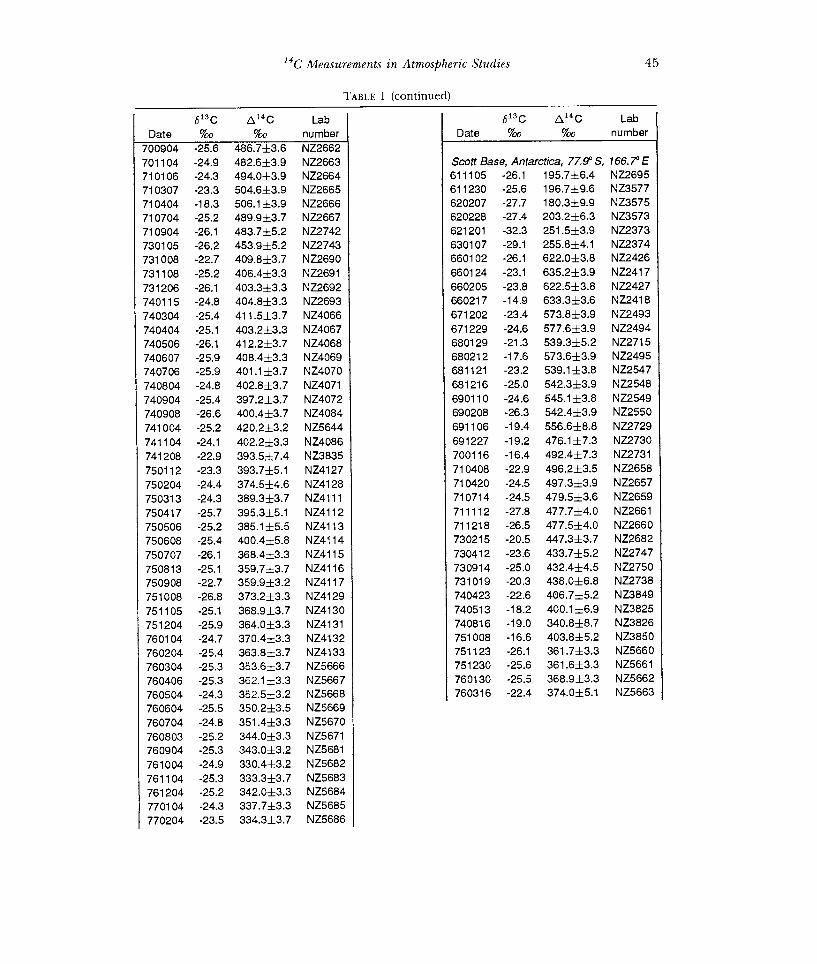
14C Measurements in Atmospheric Studies 45
TABLE 1 (continued)
6130 &4C Lab Date %o %o
700904 -25.6 486.7±3.6 701104 -24.9 482.6±3.9 Base, Antarctica, 77.9° S, 166.7° E 710106 -24.3 494.0±3.9 710307 -23.3 504.6±3.9 710404 -18.3 506.1±3.9 710704 -25.2 489.9±3.7 710904 -26.1 483.7±5.2 730105 -26.2 453.9±5.2 731008 -22.7 409.8±3.7 731108 -25.2 406.4±3.3 131206 -26.1 403.3±3.3 740115 -24.8 404.8±3.3 740304 -25.4 411.5±3.7 740404 -25.1 403.2±3.3 740506 -26.1 412.2±3.7 740607 -25.9 408.4±3.3 740706 -25.9 401.1±3.7 740804 -24.8 402.8±3.1 740904 -25.4 397.2±3.7 740908 -26.6 400.4±3.7 741004 -25.2 420.2±3.2 741104 -24.1 402.2±3.3 741208 -22.9 393.5±7.4 750112 -23.3 393.7±5.1 750204 -24.4 374.5±4.6 750313 -24.3 389.3±3.7 750417 -25.7 395.3±5.1 750506 -25.2 385.1±5.5 750608 -25.4 400.4±5.8 750707 -26.1 368.4±3.3 750813 -25.1 359.7±3.7 750908 -22.7 359.9±3.2 751008 -26.8 373.2±3.3 751105 -25.1 368.9±3.7 751204 -25.9 364.0±3.3 760104 -24.7 370.4±3.3 760204 -25.4 363.8±3.7 760304 -25.3 353.6±3.7 760406 -25.3 362.1±3.3 760504 -24.3 352.5±3.2 760604 -25.5 350.2±3.5 760704 -24.8 351.4±3.3 760803 -25.2 344.0±3.3 760904 -25.3 343.0±3.2 761004 -24.9 330.4±3.2 761104 -25.3 333.3±3.7 761204 -25.2 342.0±3.3 770104 -24.3 337.7±3.3 770204 -23.5 334.3±3.7 NZ5686
46
600
400
200
0
600 -
400 E-
200
55 60
M R Manning et al
YY
65 70
Year
75 80
A
85
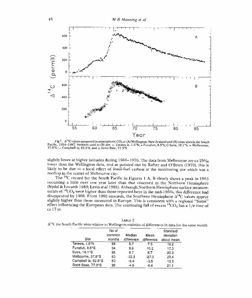
Fig 1. L' 4C values measured in atmospheric CO2 at (A) Wellington, New Zealand and (B) other sites in the South Pacific, 1954-1987. Symbols used in (B) are: + Tarawa Is,1.5°N; * Funafuti, 8.5°S; 0 Suva, 18.1 °S; x Melbourne, 37.8°S; 0 Campbell Is, 52.5°S; and Scott Base, 77.9°S.
slightly lower at higher latitudes during 1966-1976. The data from Melbourne are ca 25°/ lower than the Wellington data, and as pointed out by Rafter and O'Brien (1970), this is likely to be due to a local effect of fossil-fuel carbon at the monitoring site which was a rooftop in the center of Melbourne city.
The 14C record for the South Pacific in Figures 1 A, B clearly shows a peak in 1965 occurring a little over one year later than that observed in the Northern Hemisphere (Nydal & Lovseth 1983; Levin et al 1985). Although Northern Hemisphere surface measure- ments of 14002 were higher than those reported here in the mid-1960s, this difference had disappeared by 1968. From 1980 onwards, the Southern Hemisphere a14C values appear slightly higher than those measured in Europe. This is consistent with a regional "Suess" effect influencing the European data. The continuing fall of excess 14002 has a lie time of ca 17 yr.
TABLE 2 Z' 4C for South Pacific sites relative to Wellington statistics of differences in data for the same month
No of Standard
Site common months difference difference about mean
Tarawa,1.5°N 58 8.7 Funafuti, 8.5°S 34 8.6 Suva, 18.1°S 86 8.7 Melbourne, 37.8°S 60 -22.3 Campbell Is, 52.5°S 50 -6.4 Scott Base, 77.9°S 29 -4.5 -6.6 21.1

l4C Measurements in Atmospheric Studies 47
The seasonal structure in the region of the peak Southern Hemisphere values is much less pronounced than for Northern Hemisphere data. This, together with the later arrival of the peak in the Southern Hemisphere, is consistent with the fact that most of the release of
C from nuclear weapons testing occurred in the Northern Hemisphere. Further, it is well established (Telegadas 1971) that most of the 14C inventory produced by nuclear tests was located in the stratosphere by the mid-1960s. Figure 2 shows this stratification of the 14C
inventory between the stratosphere and troposphere by comparing surface data (Levin et al 1985; this work), with tropospheric and stratospheric data (Telegadas 1971).
ANALYSIS OF 14C02 DATA
We average all the data (usually just one value) available for Wellington in each month in order to obtain a time series spanning 391 months with 104 missing values. The missing data are fairly evenly distributed through the record and so are unlikely to bias the following analysis.
In order to extract a seasonal component, we must determine a smooth trend in the data about which the seasonal variation occurs. There are many procedures for doing this (eg, Cleveland Freeny & Graedel 1983; Enting 1987). The methods used here are based on "loess" smoothing (Cleveland 1979) and the "STL" procedure for seasonal and trend decomposition (Cleveland & McRae 1989).
Loess smoothing determines a smoothed value at each point in the series from a window of a fixed number of nearest neighbors. The smoothed value is determined by fitting a straight line to the data window using weights that decrease with distance from the subject point. Both loess smoothing and the STL procedure are robust with respect to outliers, ie,
104
E 3 10
a
102
55 60 65 70
Year
75 80 85
Fig 2. values in the stratosphere and at the earth's surface shown as smooth spline curves fitted to available data; the upper two curves are for the stratosphere and the lower two for the surface; - denotes Northern Hemisphere and Southern Hemisphere. Based on stratospheric data from Telegadas (1971), Northern Hemisphere surface data from Levin et al (1985) and Southern Hemisphere surface data from this work.

48 M R Manning et al
outlier points are identified by an initial calculation, their weights are reduced and the calculation repeated. The STL procedure determines the seasonal and trend components simultaneously with a consistent philosophy of the structure of each. The trend component is determined by loess smoothing of the data minus the seasonal component, the latter being determined for each calendar month by loess smoothing of the data minus the trend component. STL allows arbitrary variation of the seasonal component from month to month within the year (in contrast to band pass filtering methods) but ensures small variation in the seasonal cycle from year to year.
There are inherent difficulties in separating seasonal and trend components for both the rapid rise in Q14C values during the early 1960s and the following decay. Further, the relative distribution of 14C throughout the atmosphere may have been significantly altered by the very large tesss of the early 1960s. Thus, in order to determine a consistent and slowly varying seasonal component, we have limited the analysis to 1966 onwards.
The STL procedure does not allow for missing data, so missing values have been interpolated by fitting a Reinsch (1967) spline to the data, and adjusting the tension of the spline so that the number of sign changes in residuals agrees with that expected for a random sequence. We have tried alternative procedures for interpolating missing data which do not significantly affect the results. Figures 3A, B, C, show the trend, seasonal and remainder components. The seasonal component shows a cycle of decreasing amplitude with some evidence of a phase change in the latter part of the record.
Up to 1980, the cycle has a maximum in March and a minimum in August; a negative anomaly occurs in December. The amplitude of the cycle decreases steadily from a peak-to- peak range of 20%0 in 1966 to 3%0 in 1980. From 1966-1975, while the shape of the cycle is roughly constant, the amplitude decays exponentially with a lie time of 12 yr. From 1980 onwards, a different cycle emerges with an amplitude of ca 5%0, a maximum in July- August
600
E L a) 0
U
4
400
200
10
0
-10
20
0
-20
A. trend
II , IIII lid IIII 111
III I I I I II
B. seasonal
IIII.. I IIII., I Illlill I IIII,1. I .111111 I ,111.11 i ,111.11 1 1111,11 I, 1111111 .il 1111.1.,.1, ..1 .II....,I ,1111 ,I.IIII I I
. IIII I ,
11 VIII IIII
IIII II
I I 1 11 I 1 illu Ilqu
III J.I_III,IIIlIIIIII I III.III
11.1 I
65 70
C. remainder
II,LI
I,I I ., I
I I,
111.1111. ,1
J I .11111
I III.
I. IIII ..,I III. III, 11 11/11/1.
I VIII.
I ..II II,
I I
75 80 85
Year Fig 3. The (A) smooth trend, (B) seasonal and (C) remainder components of the Wellington &40 data record
determined by the STL procedure as discussed in the text.

140 Measurements in Atmospheric Studies 49
and minimum in January. If present, this would have been masked in the earlier part of the record by the larger decaying cycle.
A direct indication of the change in the seasonal cycle can be seen by plotting the differences of the original data from a smooth trend, against a calendar month. Figures 4A, B show such "month-plots" of differences from the smooth trend, in the periods 1966- 1977 and 1981-1987. Horizontal bars show the mid-mean (mean of values between the upper and lower quartiles) of all data for a given month. Individual data values are shown by a spike from the mid-mean for the corresponding month. The contrast in the annual cycle for these two periods confirms that the change in the seasonal cycle is not an artifact of the interpolation or outlier rejection techniques used with the STL procedure.
Finally, we note that the seasonal cycles at the other South Pacific sites are not well determined by our data, and for some months the differences between sites are large compared with errors due to counting statistics. These appear often enough to suggest that regional variations in "CO2 may be as large as
INTERPRETATION OF 14C02 SEASONAL AND TREND VARIATION
The overall decline in atmospheric 14002 has been studied extensively in many analyses of the global carbon cycle (Oeschger et al 1975; Enting & Pearman 1983). This decline is
predominantly determined by the rate of exchange of carbon between the atmosphere and the ocean, and is one of the best determinants of that exchange rate.
Although the seasonal cycle in atmospheric 14C02 has not been well researched, seasonal cycles in other "bomb"-produced radionuclides, particularly 905r and 3H, are influenced by seasonal changes in transport of stratospheric air into the troposphere. The transport of gaseous tracers such as "CO2 is by advection and diffusion, whereas for other radionuclides particulate deposition and rainout phenomena are dominant (Sarmiento &
Gwinn 1986; Schell, Sauzay & Payne 1974). Thus, differences between the seasonal cycle of '4C02 and other fallout species are expected.
to
E -10
-10
-20
L
[1
B
Jan Feb Mar Apr May Jun Jul Aug Sep Oct Nov Dec
Fig 4. Seasonal cycles of differences between 0140 data and their smooth trend. Data are grouped by calendar month and shown as spikes from the mid-mean, (A) for period 1966-1977 and (B) for period 1981-1987.

50 M R Manning et al
Factors other than transport from the stratosphere also contribute to seasonal variation in 14CO2. Levin (1985) reports variations at a European site due to seasonal changes in the release of fossil-fuel CO2, and at an Antarctic site due to seasonal changes in ocean- atmosphere exchange.
The seasonal cycle from 1966 to 1980 is consistent with a seasonal variation in the transfer of "bomb" 14002 from the stratosphere to the troposphere. The decay in the amplitude of this cycle is then explained by the depletion of the stratospheric inventory. Because mixing within the Southern Hemisphere troposphere occurs within a few months, we assume that the amplitude of the seasonal component seen at the surface is proportional to the amount of 14CO2 transferred from stratosphere to troposphere in the previous few months. If this is assumed to be proportional to the 14CO2 inventory in the stratosphere, modulated by the seasonally varying exchange rate, then the 12-yr decay time of the seasonal cycle is equal to the mean residence time for stratospheric CO2.
This estimate of stratospheric mean residence time is longer than the value of 7.0 yr (half-life of 58 months) derived by Telegadas (1971) from measurements of 14C in the stratosphere up to 1969. This earlier data may reflect a residence time for just the lower part of the stratosphere. The value derived here is closer to an alternative estimate of 10 yr for the mean residence time of air in the stratosphere based on energy and mass flux (Walker 1977).
COMPARISON OF '4001 DATA WITH ATMOSPHERIC TRANSPORT MODELS
Modeling of tracer transport in the atmosphere due to advection and diffusion has progressed considerably in recent years (Mahlman, Levy & Moxim 1980; Golombek & Prinn 1986). Models that incorporate consistent global circulation and realistic (if approximate) climatology can now be used to predict tracer concentrations. This approach is preferable to inferring atmospheric transport from tracer data alone.
We now present some results using a two-dimensional model for atmospheric transport (Plumb & Mahlman 1987; Plumb & McConalogue 1988) which is a zonally averaged version of a larger three-dimensional global circulation model (GCM) (Mahlman & Moxim 1978). The zonally averaged version gives the same net tracer transport as the three-dimensional model, but requires much less computer time. A resolution of 2.4° in latitude and 10 vertical levels extending to the l OmBar level (33km) are used.
The vertical diffusion coefficients at the lowest two layers were increased to 8m2s-1 (bottom level) and 6m2s-1 (next lowest level), based on other work using this model for determining seasonal variation of atmospheric CO2 concentrations (Plumb, pers commun). Otherwise the fields determining atmospheric transport are as determined from the three-dimensional GCM.
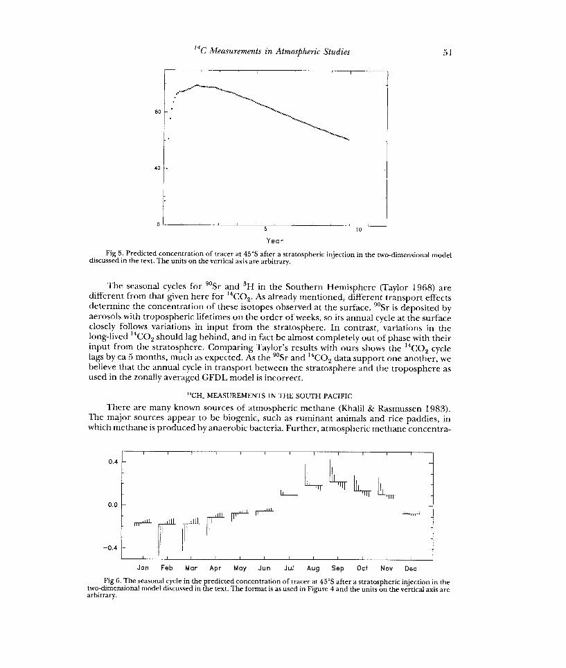
To relate our South Pacific 14CO2 data with this model, it was run from an initial condition where a tracer is injected instantaneously with uniform concentration throughout the lower three grid layers of the stratosphere representing pressure levels 110, 65 and 38mbar. The only sink for the tracer is at the surface, where there is a uniform sink strength set to give approximately the observed overall decay rate from 1966 onwards. Figure 5 shows the tracer concentration at 45°S predicted by the model. Note that results for the first two years are sensitive to the artificial initial conditions. Figure 6 shows a month plot, in the same format as Figure 4A, of the seasonal component of this predicted time series, extracted using the STL procedure after removal of the first two years of data.
There is a significant discrepancy in phase between the predicted seasonal cycle in Figure 6 and the observed one in Figure 4A. The model predicts that the concentration of a tracer injected into the stratosphere will peak in September and reach a minimum in January, almost totally out of phase with the observed result. This implies that either the seasonality of vertical transport in the model is incorrect or the observed seasonal cycle in 14CO2 is determined by effects other than seasonality in transport from the stratosphere.
14C Measurements in Atmospheric Studies
80
40
5
Year
10
51
Fig 5. Predicted concentration of tracer at 45°S after a stratospheric injection in the two-dimensional model discussed in the text. The units on the vertical axis are arbitrary.
The seasonal cycles for 90Sr and sH in the Southern Hemisphere (Taylor 1968) are different from that given here for 14C02. As already mentioned, different transport effects determine the concentration of these isotopes observed at the surface. 905r is deposited by aerosols with tropospheric lifetimes on the order of weeks, so its annual cycle at the surface closely follows variations in input from the stratosphere. In contrast, variations in the long-lived 14C02 should lag behind, and in fact be almost completely out of phase with their input from the stratosphere. Comparing Taylor's results with ours shows the 14C02 cycle lags by ca 5 months, much as expected. As the 905r and 14C02 data support one another, we believe that the annual cycle in transport between the stratosphere and the troposphere as used in the zonally averaged GFDL model is incorrect.
14CH4 MEASUREMENTS IN THE SOUTH PACIFIC
There are many known sources of atmospheric methane (Khalil & Rasmussen 1983). The major sources appear to be biogenic, such as ruminant animals and rice paddies, in which methane is produced by anaerobic bacteria. Further, atmospheric methane concentra-
0.4
F'
0.0
-0.4
L L J
Jan Feb Mar Apr May Jun Jut Aug Sep Oct Nov Dec
Fig 6. The seasonal cycle in the predicted concentration of tracer at 45°S after a stratospheric injection in the two-dimensional model discussed in the text. The format is as used in Figure 4 and the units on the vertical axis are arbitrary.
52 M R Manning et al
tions have been increasing at ca 1 %/a over recent decades, suggesting an increasing source strength.
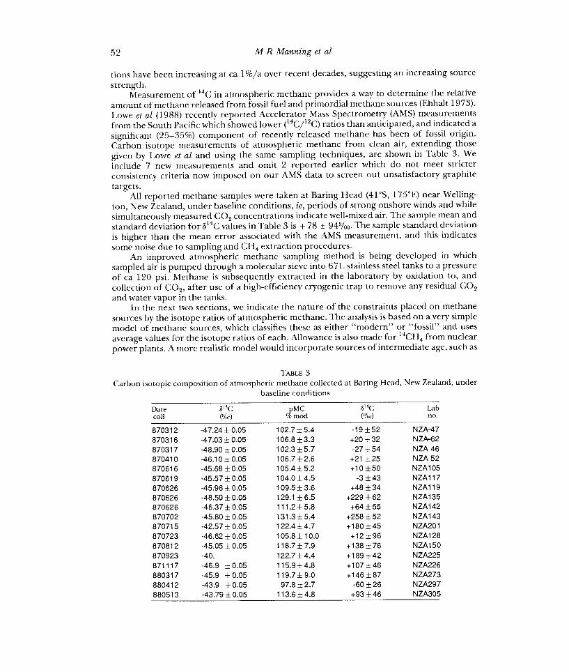
Measurement of 14C in atmospheric methane provides a way to determine the relative amount of methane released from fossil fuel and primordial methane sources (Ehhalt 1973). Lowe et al (1988) recently reported Accelerator Mass Spectrometry (AMS) measurements from the South Pacific which showed lower (14C/12C) ratios than anticipated, and indicated a significant (25-35%) component of recently released methane has been of fossil origin. Carbon isotope measurements of atmospheric methane from clean air, extending those given by Lowe et al and using the same sampling techniques, are shown in Table 3. We include 7 new measurements and omit 2 reported earlier which do not meet stricter consistency criteria now imposed on our AMS data to screen out unsatisfactory graphite targets.
All reported methane samples were taken at Baring Head (41 °S, 175°E) near Welling- ton, New Zealand, under baseline conditions, ie, periods of strong onshore winds and while simultaneously measured CO2 concentrations indicate well-mixed air. The sample mean and standard deviation for b14C values in Table 3 is + 78 ± 94%. The sample standard deviation is higher than the mean error associated with the AMS measurement, and this indicates some noise due to sampling and CH4 extraction procedures.
An improved atmospheric methane sampling method is being developed in which sampled air is pumped through a molecular sieve into 67L stainless steel tanks to a pressure of ca 120 psi. Methane is subsequently extracted in the laboratory by oxidation to, and collection of C02, after use of a high-efficiency cryogenic trap to remove any residual CO2 and water vapor in the tanks.
In the next two sections, we indicate the nature of the constraints placed on methane sources by the isotope ratios of atmospheric methane. The analysis is based on a very simple model of methane sources, which classifies these as either "modern" or "fossil" and uses average values for the isotope ratios of each. Allowance is also made for 14CH4 from nuclear power plants. A more realistic model would incorporate sources of intermediate age, such as
TABLE 3
Carbon isotopic composition of atmospheric methane collected at Baring Head, New Zealand, under baseline conditions
Date b MC coil (%) % mod
870312 -47.24+0.05 102.7±5.4 870316 -47.03 f 0.05 106.8 f 3.3 f 32 870317 -48.90 f 0.05 102.3 f 5.7 f 54 46 870410 -46.10±0.05 106.7±2.6 ±25 52 870616 -45.68±0.05 105.4±5.2 870619 -45.57±0.05 104.0±4.5 43 870626 -45.96 ± 0.05 109.5 f 3.6 f 34 870626 -48.59 f 0.05 129.1 f 6.5 f 62 870626 -46.37 f 0.05 111.2±5.8 f 55 870702 -45.80 f 0.05 131.3±5.4 f 52 870715 -42.57 f 0.05 122.4±4.7 870723 -46.62±0.05 105.8±10.0 870812 -45.05 ± 0.05 118.7 ± 7.9 76 870923 -40. 122.7±4.4 871117 -46.9 ±0.05 115.9±4.8 880317 -45.9 ± 0.05 119.7 f 9.0 880412 -43.9 ±0.05 97.8±2.7 f 26 880513 -43.79 f 0.05 113.6±4.8 46 NZA305

14C Measurements in Atmospheric Studies 53
swamps, and use direct isotope measurements of a range of sources with appropriate source strengths. However, the simpler analysis gives an upper estimate for the proportion of methane derived from fossil fuel, and demonstrates the sensitivity of such estimates to some general parameters of atmospheric transport and chemistry.
A TWO BOX ATMOSPHERE MODEL FOR CH4 ISOTOPES
To interpret the 14CH4 data above, we use a model treating the two hemispheres as well-mixed boxes with mass balanced exchange and consider the inventories of CH4,13CH4 and 14CH4 separately. The changes in inventories are related to fluxes by
d
dt Ch Qh - k (Ch - Ch-) - ACh
=13 h Qh-k(13Ch- dt
f14C =14 h Qh-k(14Ch-
where:
h h` Ch,
13Ch and 14Ch
Qh, 13Qh and 14Qh
k
A
E
13Ch,) - EA 13Ch
14C h) - E2A 14Ch (1)
labels the hemisphere S or N; labels the alternate hemisphere; are the inventories of CH4,13CH4 and 14CH4 in hemisphere h; are the source fluxes of CH4,13CH4 and 14CH4 into hemisphere h; is the inter-hemispheric fractional exchange coefficient, taken to be (2
yr)-1; is the inverse mean life of CH4, taken to be (9.6 yr)-1 following Prinn et al (1987). Note that the small difference between the mean life of 12CH4
and CH4 is ignored here; is the kinetic isotope effect coefficient, taken to be 0.990 ± 0.007 following Davidson et al (1987) ((k13/k12) in their notation).
The solution of these equations can be written as
CN(t) + C3(t) _ (QN(x) + Qs(x)) dx
CN(t) - Cs(t) = t
e(2k+a)(x-t) (QN(x) - Qs(x)) dx (2)
with similar equations for 13C and 14C.
The inventories are sensitive to the source flux terms Q only over the last few mean lifetimes of CH4, ie, over the last few decades. For the recent past, we assume that the total CH4 source flux has increased exponentially at 1%/a and further that the regional distribu- tion of fluxes has remained constant. Then
QN (x) + Qs (x) = Qtot eµ(x-1987)
QN(x) - Qs (x) _ Qtot e t(x-1987)
where:
(3)
is the total CH4 release/a in 1987; is the excess release in the Northern Hemisphere over the Southern Hemisphere;
µ is the exponential increase rate, taken as 0.01.
54 M R Manning et al
Evaluating the appropriate integrals in equation (2) we have for the total CH4 inventories:
CN(t) + Cs(t) _ Qtot eµ(t-1987)
2k
Q Qtot eµ(t-1987) . GN(t) _ Gs(t) _
+ A + µ (4)
Assuming, in 1987, a mean atmospheric CH4 concentration of 1670 ppb, and an interhemi- spheric difference of 90 ppb (Steele et al 1987; Fraser et al 1986), an atmospheric mass of 1.82 x 10²⁰ moles, and values of A, µ and k already quoted, we have
Qtoc = 3.47 x 10¹³ moles/a
L\Qtot = 0.91 x 10¹³ moles/a.
To determine the inventories of 13CH4 and 14CH4, we assume that the CH4 source can be separated into fossil and modern carbon components each having different isotope ratios, which together with the relative proportions of the two sources, have not changed in recent decades. Then
13Qh(t) = (1 + a 13Sfos + (1 - a) 13Smod) 13RoQh(t) (5)
where:
a is the fossil carbon fraction of the total CH4 source 13R0 is the (13C/12C) ratio of the PDB standard 138
f0s is the 813 C PDB of the fossil carbon CH4 source 13amod is the 813 C PDB of the modern carbon CH4 source.
The inventories resulting from these fluxes are given by
13 13 = 13 1 _ a 13R Qtot
eµ(t-1987) GN(t) + CS(t) (1 + a' ofos + ( ) mod) 0 EA + µ
13 _ 13 = 13 _ 13 13R0 tot eµ(t-1987) CN (t) CS (t) (1 + a ofos + (1 a) omod)
2k + fx +t (6)
Turning next to 14CH4, note that the fossil carbon source has no contribution to Qh, but that a nuclear power source (Povinec, Chudy & Sivo 1986) must be considered even though this is a negligible source of total CH4. Thus
14QN(t) = (1 - a) (1 + 145mod(t)) 14R0QN(t) + 14QNuc(t)
14QS(t) = (1 _ a) (1 + 148mod(t))14ROQS(t) (7)
where:
14Smod(t) 14R 0
14 QNuc(t )
is the mean 814C of the modern carbon source is the (14C/12C) ratio of the modern 14C standard (0.95 NBS oxalic acid), taken to be 1.176 x 10⁻¹² following Karleen et al (1964) and is the nuclear power source term.

14C Measurements in Atmospheric Studies 55
This leads to
14CN(t) + '4C (t) = f eEZA(x-t) [(1 - a) (1 + '4ROQtot 1987) + 14QNuc(x)J dx l1 II
1 4CN(t) - 14Cs(t) = t
e(2k+E2a)(x-t) [(1 - a)
(1 + 14bmod) 14R°
LQtot eµ(x-1987) + 14QNuc(x)] dx. (8)
The value of 14bmod(t) has changed with time due to changes in the 814C of atmospheric CO2 which provides the carbon from which the modern CH4 is derived. We assume a residence time of one year between carbon photosynthesis and methane production, and correct for fractionation to b13C of - 65%o (note this is the inferred value of b13C for the modern carbon CH4 source-see below). Thus
2 1 - 65%0
(1 + 14amod(t)) _ - 0
/(1 + Z 4Catm(t - 1)) 1 25 oo
(9)
where Z14Catm(t) is the atmospheric L14C value for time t. In order to estimate this last term, we use an average of the atmospheric 14C data of Levin et al (1985) representing the Northern Hemisphere, and the atmospheric 14C data given here representing the Southern Hemisphere. Where the Northern Hemisphere data is missing we assume it is the same as the Southern Hemisphere, and prior to 1955 we assume a constant value of - 20%0. The lower limit of the integration range in equation (8) is taken as 1940, as the integrands become negligible prior to this. Numerical integration then produces
1987 (1 + e(E2a+µ)(x-1987) dx = 10.718
1987 (1 + 14Smod) e(2k+E2A+µ)(x-1987) dx = 1.0037. (10)
Levin (pers commun) has estimated the nuclear power term QNUC(t) and we use her estimates here. In 1987 the estimated release rate is 1100 Ci/a, corresponding to 17.6 moles of 14CH4/a. This is more conveniently expressed as 0.4314R0Qt0t, based on the value of Qtot given above. Using Levin's exponential growth rates, we have
QNUC(t) = 0.4314RoQt0 t e016(t-1987) for t = 1975 to 1987,
QNUC(t) = 0.06314RoQt0 t eo.26(t-1975) for t = 1969 to 1975 and
QNuc(t) = 0, fort < 1969. (11)
The integrals in equation (8) involving QNuc can now be evaluated as
J1987 E2A(-) 14 e''987 QNuc (x) dx = 1.6153 R 0 Qcoc
_198 e(2k+E2A)(x-1987) QNUC (x) dx = 0.340714R Q. (12)
INTERPRETATION OF 14CH4 DATA
We can now calculate a, the fossil carbon fraction, from observed b14C values for atmospheric CH4. To summarize, values of k, A, µ, and mean hemispheric CH4 concentra- tions are used to estimate Qt ?t
and OQtot; then estimates of E,14Smod(t) and 14QNUC(t) are used to calculate the hemispheric inventories relative to the total CH4 inventory in terms of

56 M R Manning et al
an unknown a. Finally, we relate the inventory ratio to the observed 514C using
14C S = 1480 (1 + b14Cobs) (13)
CS
giving an equation which is solved for a. With the parameters values given above, this leads to
1.226 (1 - a) + 0.150 = (1 + 814Cobs)
where 1.226 is the value of (1 + b14C) that would arise if the only source was from modern carbon, and 0.150 is the shift due to the nuclear power source. From these values we have a = 0.243.
Consistency of the 13CH4 and 14CH4 budgets is now considered. Equation 6 predicts a slight difference in the S13C values of CH4 for the two hemispheres. This arises because the larger source term in the Northern Hemisphere leads to a net export of aged (and, due to the kinetic oxidation effect, heavier) CH4 to the Southern Hemisphere. Ignoring this very small effect, we have
13 1 a 13b _ a 13b
1 -- b Cobs fos + (1 ) mod ) µ
or, to a good approximation
a13Cobs ' a13bfos + (1 - a) 13bmod + (14)
If the fossil CH4 source is assumed to be entirely from fossil fuels then the value of 13bfos should be ca - 300/oo and, in order to explain b13Cobs = - 47%o, we must have 13bmod - 65%0. Although this inferred value is slightly lighter than that used in other CH4 budgets (eg, Tyler, Blake & Rowland 1987; Stevens & Engelkemeir 1988), it is well within the range of 813C values of the known sources of modern carbon CH4. Equation 13, based on observed 14C values, gives a more reliable estimate of a than Equation 14, based on 13C values, because of the considerable uncertainty in 138mod in the latter. Thus, we have used equation 13 to determine a and equation 14 to check consistency.
To estimate the sensitivity of a to the parameters of this two-box model, we consider the effect of making variations in these parameters of the order of their uncertainties. This leads to
parameters as described above a = 0.243
k changed from (2 yr) -1 to (1 yr)
-1 a = 0.255
A changed from (9.6 yr) -1 to (8.6 yr)
-1 a = 0.252
E changed from 0.990 to 0.997 a = 0.233
Q.Nuc reduced to half equation (11) a = 0.182
b14Cobs changed from + 78% to + 172% a = 0.166.
This shows that a is not very sensitive to the methane lifetime estimate, the kinetic isotope effect or the inter-hemispheric exchange time. Yet it is sensitive to the magnitude of the nuclear power source term, and to the value of 14bobs. The estimated growth rate of 17%/a in the total nuclear power 14CH4 should cause a significant increase in the b14C of atmospheric CH4. The figures used in the previous section imply an increase in the Southern Hemisphere of ca 25%o/a and, provided the fossil carbon fraction a is not also increasing, this should be clearly measurable after 2 to 3 years of measurements.
A more detailed calculation of the transport of methane between the hemispheres has been carried out using the zonally averaged atmospheric transport model already described.
'4C Measurements in Atmospheric Studies 57
When the model is run with a northern mid-latitude tracer source and a uniformly distributed sink corresponding to a tracer lifetime of 10 yr, the difference between the predicted values of the tracer concentrations at 45°N and 45°S corresponds to a 2.5-yr inter-hemispheric exchange time. This supports the value of k used above.
CONCLUSION
Our 32-yr record of atmospheric 14C02 measurements in the South Pacific covers nearly all the period in which atmospheric 14C has been influenced by nuclear weapons testing, and begins with Q14C values below zero. Since 1966 the decrease of this "bomb" carbon in the atmosphere has roughly followed an exponential decay with a 1/e time of 17 yr. From 1966-1977, the 14002 data show a small latitudinal variation, and a definite seasonal cycle peaking in February. This seasonal cycle in "CO2 is believed due to seasonal changes in the rate of transport of "bomb" carbon from the stratosphere and is consistent with the cycle of other fallout products. The cycle decayed in amplitude with a 1/e time of 12 yr, which is inferred to be the mean residence time for CO2 in the stratosphere.
A two-dimensional model of atmospheric transport based on a three dimensional general circulation model predicts a seasonal cycle in the arrival of a tracer injected into the stratosphere, but the phase of the predicted cycle disagrees with that observed for "CO2. It would seem that stratosphere-to-troposphere transport is not estimated correctly in the model.
An analysis of 14CH4 data has shown how these can be used to estimate the fraction of atmospheric methane derived from fossil carbon. A major uncertainty in this estimate appears to be the contribution of nuclear power plants to 14CH4 in the atmosphere. However, comparable measurements in both hemispheres over a number of years should enable the nuclear power source of CH4 to be better determined.
ACKNOWLEDGMENTS
The atmospheric "'CO2 data presented here are the result of the work of many people. We wish to acknowledge the contribution of M K Burr, who was responsible for maintaining our gas counters for much of the period covered. Sampling at the Wellington site was done by the staff of the New Zealand Post Office Makara radio station; at the South Pacific island sites, by meteorological observers from the New Zealand Meteorological Service; at Scott Base, by staff of the Antarctic division, DSIR, and at Melbourne, by E D Gill of the National Museum of Victoria. We are grateful for the assistance of all these people.
R A Plumb kindly provided the source code and transport coefficients for the zonally averaged model of atmospheric transport, and his support and guidance in the use of this model are much appreciated. We would also like to thank W S Cleveland for supplying code for his STL procedure. Finally, we would like to ay tribute to T A Rafter, who had the foresight to begin measurements of atmospheric 4C02 in New Zealand, and who recog- nized the importance of extending these to other South Pacific sites many years ago.
REFERENCES
Cleveland, W S 1979 Robust locally weighted regression and smoothing scatterplots. Jour Am Statistical Assoc 74: 829-836.
Cleveland, W S, Freeny, E and Graedel, T E 1983 The seasonal component of atmospheric CO2: Information from new approaches to the decomposition of seasonal time series.Jour Geophys Research 88: 10934-10946.
Cleveland, W S and McRae,J E 1989 The use of loess and STL in the analysis of atmospheric CO2 and related data. In Elliott, W P, ed, The statistical treatment of CO2 data records. NOAA Tech Memo ERL ARL-173, Silver Spring, Maryland.
Davidson, J A, Cantrell, C A, Tyler, S C, Shetter, R E, Cicerone, R J and Calvert, J G 1987 Carbon kinetic isotope effect in the reaction of CH4 with H0. Jour Geophys Research 92: 2195-2199.
Ehhalt, D H 1973 Methane in the atmosphere. In Carbon and the biosphere. Brookhaven symposium in biology, 24th, Proc. Upton, New York, USAEC, CONF-720510.
Enting, I G 1987 On the use of smoothing splines to filter CO2 data. Jour Geophys Research 92: 10977-10984. Enting, I G and Pearman, G I 1983 Refinements to a one-dimensional carbon cycle model. CSIRO Div Atmos
Research tech paper 3. Fraser, P J, Hyson, P, Rasmussen, R A, Crawford, A J and Khalil, M A K 1986 Methane, carbon monoxide and
methylchloroform in the Southern Hemisphere. JourAtmos Chem 4: 3-42.
58 M R Manning et al
Golombek, A and Prinn, R G 1986 A global three-dimensional model of the circulation and chemistry of CFC13, CF2C12, CH3CC13, CCl4, and N20. Jour Geophys Research 91: 3985-4001.
Heimann, M and Keeling, C D 1986 Meridional eddy diffusion model of the transport of atmospheric carbon dioxide, l . Seasonal carbon cycle over the tropical Pacific ocean. Jour Geophys Research 91: 7765-7781.
Karlen, I, Olsson, I, U, Kallberg, P and Kilicci, S 1964 Absolute determination of the activity of two 14C dating standards. Arkiv Geofysik 4: 465-471.
Keeling, C D, Mook, W G and Tans, P P 1979 Recent trends in the '3C/12C ratio of atmospheric carbon dioxide. Nature 277: 121-123.
Khalil, M A K and Rasmussen, R A 1983 Sources, sinks and seasonal cycles of atmospheric methane. Jour Geophys Research 88: 5131-5144.
Lal, D and Peters, B 1962 Cosmic ray produced isotopes and their application to problems in geophysics. Progress in elementary particle and cosmic ray physics. Amsterdam, North Holland 6: 1-74.
Levin, I (ms)1985 Atmospheric CO2 in continental Europe-An alternative approach to clean air CO2 data. Paper presented at IAMAP mtg, Atmospheric carbon dioxide its sources, sinks, and global transport, Kandersteg, Switzerland.
Levin, I, Kromer, B, Schoch-Fischer, H, Bruns, M, Munnich, M, Berdau, D, Vogel, J C and Munnich, K 01985, 25 years of tropospheric 14C observations in central Europe. Radiocarbon 27(1): 1-19.
Logan, J A, Prather, M J, Wofsy, S C and McElroy, M B 1981 Tropospheric chemistry: A global perspective. Jour Geophys Research 86: 7210-7254.
Lowe, D C, Brenninkmeijer, C A M, Manning, M R, Sparks, R and Wallace, G 1988 Radiocarbon determination of atmospheric methane at Baring Head, New Zealand. Nature 332: 522-525.
Mahlman, J D, Levy, H and Moxim, W J 1980 Three dimensional tracer structure and behaviour as simulated in two ozone precursor experiments. Jour Atmos Sci 37: 655-685.
Mahlman, J D and Moxim, W J 1978 Tracer simulation using a global general circulation model: results from a midlatitude instantaneous source experiment. Jour Atmos Sci 35:1340-1374.
Nydal, R and Lovseth, K 1983 Tracing bomb 14C in the atmosphere 1962-1980. Jour Geophys Research 88: 3621- 3642.
Oeschger, H, Siegenthaler, U, Schotterer, U and Gugelmann, A 1975 A box diffusion model to study the carbon dioxide exchange in nature. Tellus 27: 168-192.
Peng, T-H, Broecker, W S, Freyer, H D and Trumbore, S 1983 A deconvolution of the tree ring based 813C record. Jour Geophys Research 88: 3609-3620.
Plumb, R A and Mahlman, J D 1987 The zonally averaged transport characteristics of the GFDL general circula- tion /transport model. Jour Atmos Sci 4:298-326.
Plumb, R A and McConalogue, D D 1988 On the meridional structure of long-lived tropospheric constituents. Jour Geophys Research 93: 15,897-15,913.
Povinec, P, Chudy, M and Sivo, A 1986 Anthropogenic radiocarbon: past present and future. In Stuiver, M and Kra, R S, eds, Internatl 14C conf,12th, Proc. Radiocarbon 28(2A): 668-672.
Prinn, R, Cunnold, D, Rasmussen, R, Simmonds, P, Alyea, F, Crawford, A Fraser, P and Rosen, R 1987 Atmospheric trends in methylchloroform and the global average for the hydroxyl radical. Science 238: 945- 950.
Rafter, T A 1955 '4C variations in nature and the effect on radiocarbon dating. New Zealand Jour Sci Tech 37: 20- 38.
Rafter, T A and Fergusson, G J 1959 Atmospheric radiocarbon as a tracer in geophysical circulation problems. In United Nations peaceful uses of atomic energy, Internatl conf, 2nd, Proc. London, Pergamon Press.
Rafter, T A and O'Brien, B J 1970 Exchange rates between the atmosphere and the ocean as shown by recent C14 measurements in the south Pacific. In Olsson, I U, ed, Radiocarbon variations and absolute chronology, Nobel symposium, 1 2th, Proc. Stockholm, Almqvist & Wiksell.
Reinsch, C M 1967 Smoothing by spline functions. Num Math 10: 177-183. Sarmiento, J L and Gwinn, E 1986 Strontium 90 fallout prediction. Jour Geophys Research 91: 7631-7646. Schell, W R, Sauzay, G and Payne, B R 1974 World distribution of environmental tritium. In Physical behaviour of
radioactive contaminants in the atmosphere, IAEA and WMO symposium, Proc. Vienna, IAEA-STI/PUB/354, IAEA.
Steele, L P, Fraser, P J, Rasmussen, R A, Khalil, M A K, Conway, T J, Crawford, A J, Gammon, R H, Masarie, K A and Thoning, K W 1987 The global distribution of methane in the troposphere. Jour Atmos Chem 5: 125-171.
Stevens, C M and Engelkemeir, A 1988 Stable carbon isotopic composition of methane from some natural and anthropogenic sources. Jour Geophys Research 93: 725-733.
Stevens, C M, Krout, L, Walling, D and Venters, A 1972 The isotopic composition of atmospheric carbon monoxide. Earth Planetary Sci Letters 16: 147-165.
Stuiver, M and Polach, H A 1977 Discussion: Reporting of 14C data. Radiocarbon 19(3): 355-363. Taylor, C B 1968 A comparison of tritium and strontium-90 fallout in the southern hemisphere. Tellus 20: 559-
576. Telegadas, K 1971 The seasonal atmospheric distribution and inventories of excess carbon-14 from March 1955 to
July 1969. US Atomic Energy Comm rept HASL-243. Trabalka, J R, ed 1985 Atmospheric carbon dioxide and the global carbon cycle. US Dept Energy rept DOE/ER-
0239. Tyler, S C, Blake, D R and Rowland, F S 1987 ' 3C/12C ratio in methane from the flooded Amazon forest. Jour
Geophys Research 92: 1044-1048. Volz, A, Ehhalt, D H and Derwent, R G 1981 Seasonal and latitudinal variation of 1400 and the tropospheric
concentration of OH radicals. Jour Geophys Research 86: 5163-5171. Walker, J C G 1977 Evolution of the atmosphere. New York, MacMillan.