ocean dynamics and sediment transport measuring · pdf file ·...

International Research Journal of Engineering and Technology (IRJET) e-ISSN: 2395 -0056

Volume: 03 Issue: 02 | Feb-2016 www.irjet.net p-ISSN: 2395-0072

© 2016, IRJET | Impact Factor value: 4.45 | ISO 9001:2008 Certified Journal | 263

Ocean Dynamics and Sediment Transport Measuring Acoustic and Optical Instruments

PEARLIN SAM JINOJ T.1 SUSEENTHARAN V.2 RAMESH R.3

1 Research Scholar, Institute for Ocean Management, Anna University, Chennai – 600025, India

2 Scientist – C, National Institute of Ocean Technology, Chennai – 600100, India

3Professor, Institute for Ocean Management, Anna University, Chennai – 600025, India

---------------------------------------------------------------------***---------------------------------------------------------------------Abstract - Recently the coastal and ocean ecosystem/morphology shows great variability because of different phenomenon such as natural process and anthropogenic activities. In order to predict and ascertain the changes and variability, it’s necessary to be aware of the advanced technology. But, in oceanic environments the technology to be applied for research is little complex compared to the terrestrial environment because of the ocean nature & dynamics such as waves and other complex process such as the wind circulation, Coriolis force by earth rotation, evaporation, sinking of water in high latitude and so on. Further such process shows the dynamic change in past and present shoreline, near-along shore current circulation pattern and ocean hydrodynamics. The objective of this paper is to study the measurement techniques of ocean physical process and changes in the geo-morphology by circulation, wave parameters, bottom stress and suspended sediment concentration using new sensor technology. Measurement of near bottom velocity profiles, water particle velocity, pressure, optical and other parameters including velocity profiles, temperature, salinity, sediment size classes, sonar images and profiles will give the hydrodynamics and Sediment transport. Also by using such sensor based instruments for turbidity, pressure & continuous near bottom wave characteristic, bottom velocity etc., it gives sufficient dynamic parameters. The acoustic and optical type of sensor instrument discussed here can be used to measure all the dynamic parameters of ocean for suitable applications.

Keywords - Acoustic Doppler Current profiler (ADCP), Acoustic Doppler Velocimeter (ADV), Single & Multi-beam Echo-sounder, Acoustic signal, Optical Backscatter sensor, Optical Laser diffraction instrument

I. INTRODUCTION

The natural process of Ocean circulation, Sediment littoral movement and shoreline morphology [1] are highly complex to predict. But the dynamic nature such as unsteadiness, non-uniformity of surface water flow, the sediment movement in the different cells is rarely in an equilibrium state. Coastal process [2] is influenced by waves and tide which forces the distribution of sediment based on direction and its load movement. Such change may or may not reduce the near shore habitats [3] because of flux changes due to erosion or accretion and sedimentation. The natural effect and its forces by wind, tides can not be controlled and it paves way to Air-Sea Interaction, Coastal Circulation and Primary Production [4] in different part of Oceans.

The major dominant processes along the coastal sea in terms of erosion are i) coast destructed by the hitting waves and sediment movements ii) bed or suspended materials drift in coast and deposit iii) settlement of floating sediment particles in bed. The force and its action may not be stopped and the morphological changes happening along the coast can be altered based on different monsoon season [5]. In shallow water region, the manmade structures like port and harbour may influence seabed and its biota variation. The sediment movement will induce the larger algae from the bed and resuspension of fine grained sediments. Displacement of sediments caused by currents changes many species to habitat in restless areas by affecting the food chain. The stormy waves make a greater impact with massive zig-zag movement of total sediment particle along the coastline and away. In the marine ecosystem the suspended sediments and turbidity limits the marine habitat like clog fish gills etc. by reduction in some particular species.

Hence understanding such dynamics of coastal erosion, sedimentation and anthropogenic influences allows us to take counter measures against this factor. In order to find out the proper strategy for ensuring the influence, continuous monitoring and measurement should be done. In the recent decades more stable and realistic technologies such as optical, spatial and acoustic methods have been developed to measure such complex morphological changes. These approaches analyse and solve the actual changes in circulation and sediment movement (bed and suspended load).



© 2016, IRJET | Impact Factor value: 4.45 | ISO 9001:2008 Certified Journal | Page 1264

II. METHODS AND INSTRUMENTATION

In this study, various Optical, Acoustic and Spatial based instruments to measure the hydrodynamic and sediment transport parameters were reviewed and analysed. Table 1 shows the different sensor instrument, its method and the accuracy.

i. Acoustic Doppler Current profiler (ADCP)

ADCP has piezoelectric oscillators that measure ocean current and velocity over different depth in profiles. The doppler effect of sound waves that is caused by back scattering within the particular water column, results in the current and velocity. The variations that are obtained by transmitting sound wave frequency from some kiloHz to several Megahertz project the suitable high or low current profile. The temperature sensor for sound velocity correction, compass for relative motion, and pitch/roll sensor for vertical and horizontal movement are incorporated in the ADCP. Mounting can be distinguished in downward or upward looking to get 2D and 3D current velocity measurement. To extend battery life, the speed and direction of the current measurement at suitable pinging interval be configured by using supportive software. [6] stated the ADCP to measure the river discharge that can also be evaluated by the data obtained by current meter in different potential evaluation sites.

Table -1: Different sensor based instrument for the coastal dynamics measurement

Sensor Instrument Methods Accuracy/Range &

Sampling types

Acoustic Doppler

Velocimeter

(ADV)[7]

It records instantaneous velocity components with high

frequency at a single-point. The Doppler shift effect is used to

find velocity of particles in a remote sampling volume.

1% of measured

velocity, 0.25 cm/s

Acoustic Sand

Transport Meter

(ASTM)

It measures the sand particles in the volume by transmission

and scattering of ultrasound waves by the suspended volume. > 50 um

Acoustic

backscatter

profiling sensors

(ABS)[8]

It involves acoustic backscatter approach that makes use of the

speed of sound in water, the scattering strength of the

suspended material and the sound propagation characteristics.

Order of tens to

hundreds of microns

(10 to 500 microns)

Acoustic

Backscattering

System (ABS)[8]

It measures the sound that is scattered by sediment and

suspended materials at discrete spatial intervals that can be

programmed from around 2½ millimetres to several

centimeters.

Typically 20 µm to

2000 µm radius / 0.1

g/l to 20 g/l over 1 m,

or more over shorter

range

Multibeam

Echosounder[8]

The depth of water and the nature of the seabed can be

determined using multi-beam systems that emit sound waves of

broad acoustic fan shaped pulse from a special transducer

across the full swath.

Range(depth of

measurement) varies

from the frequency of

transducers

Optical

Backscatter

sensor[9]

It uses suitable sensors which depend on the size, composition

and shape of the suspended particles to measure turbidity and

suspended solid’s concentration by detecting infra-red light

scattered from suspended matter.

>1 kg/m3




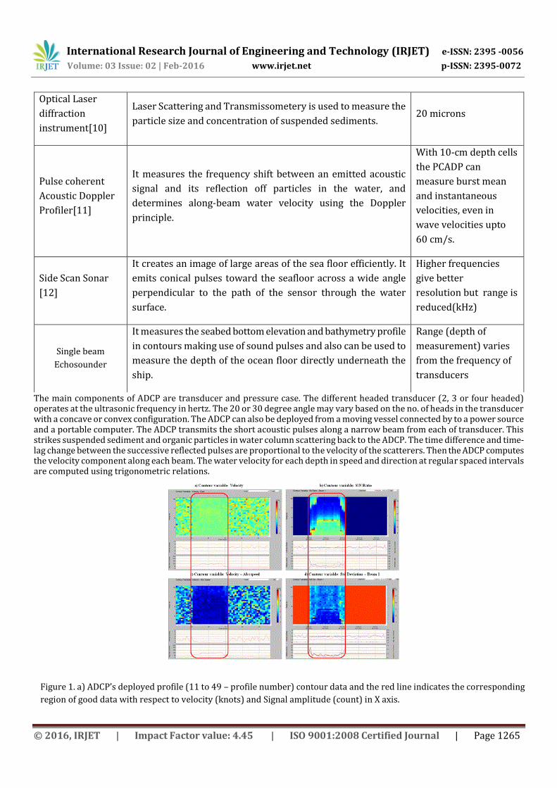
The main components of ADCP are transducer and pressure case. The different headed transducer (2, 3 or four headed) operates at the ultrasonic frequency in hertz. The 20 or 30 degree angle may vary based on the no. of heads in the transducer with a concave or convex configuration. The ADCP can also be deployed from a moving vessel connected by to a power source and a portable computer. The ADCP transmits the short acoustic pulses along a narrow beam from each of transducer. This strikes suspended sediment and organic particles in water column scattering back to the ADCP. The time difference and time-lag change between the successive reflected pulses are proportional to the velocity of the scatterers. Then the ADCP computes the velocity component along each beam. The water velocity for each depth in speed and direction at regular spaced intervals are computed using trigonometric relations.

Figure 1. a) ADCP’s deployed profile (11 to 49 – profile number) contour data and the red line indicates the corresponding

region of good data with respect to velocity (knots) and Signal amplitude (count) in X axis.

Optical Laser

diffraction

instrument[10]

Laser Scattering and Transmissometery is used to measure the

particle size and concentration of suspended sediments. 20 microns

Pulse coherent

Acoustic Doppler

Profiler[11]

It measures the frequency shift between an emitted acoustic

signal and its reflection off particles in the water, and

determines along-beam water velocity using the Doppler

principle.

With 10-cm depth cells

the PCADP can

measure burst mean

and instantaneous

velocities, even in

wave velocities upto

60 cm/s.

Side Scan Sonar

[12]

It creates an image of large areas of the sea floor efficiently. It

emits conical pulses toward the seafloor across a wide angle

perpendicular to the path of the sensor through the water

surface.

Higher frequencies

give better

resolution but range is

reduced(kHz)

Single beam

Echosounder

It measures the seabed bottom elevation and bathymetry profile

in contours making use of sound pulses and also can be used to

measure the depth of the ocean floor directly underneath the

ship.

Range (depth of

measurement) varies

from the frequency of

transducers




b) Signal to Noise ratio contour for the 1st beam with respect to velocity (knots)/Signal Amplitude and standard deviation

(cm/sec) / SNR ratio in X axis.

c) Velocity - Abs speed profile in cells (depth) contour with respect to velocity (knots) and Signal amplitude (count) in X axis.

d) Standard deviation (beam1) contour variable in cells (depth) with respect to velocity (knots)/Signal Amplitude and

standard deviation (cm/sec) / Depth average velocity (knots) in X axis

[13] states the direct measurement for vertical velocity with the traditional transducer array from the individual beam-wise measurements. The vertical velocity calculates average of four beam-wise velocities with a scaling factor to account for beam angle based on the transducer heads.

b1 to b4 are individual beam velocities and θ is the Janus angle(i.e. angle of the beam with respect to vertical). The four beam velocities are separated and if the Z-components of velocity are not uniform at four points (due to turbulence, interference of phase of an orbital wave velocity at points). The Z velocity is an average of four physically separated beam velocities and Z velocity of vertical beam is measured directly along that beam.

If the ADCP is deployed in the moving object, the moving velocity will be taken into account for the velocity computing. The ADCP can compute the speed and direction of the moving vessel object in deployment using bottom tracking methods. The current monitoring of real-time data can be done by using a specific software program. Fig.1 shows the ADCP current velocity & direction data and its S/N ratio, Standard deviation of the xyz beams of ADCP taken from Nagapattinam Coast (June 2015). The performance and accuracy of Field observation of ADCP’s shows the quality results. More accurate estimation in flow patterns using many water columns shows the thermocline and halocline scaling. ADCP can also be used to obtain the high resolution profiling of sediment transport and near-seabed velocity [14].

ii. Acoustic Doppler Velocimeter (ADV)

Doppler shift effect can be used to measure the instantaneous velocity component at a single point with a relatively high frequency. The ADV arm has one transmitter and three to four receivers as per the angle for remote sampling (120o or 90o) in a cylindrical sampling size. The quality and accuracy of the velocity data depends on the following the receiver velocity component, the Signal strength value, the Signal-to-Noise (SNR) ratio and the correlation value. Without proper calibration of suspended sediment concentration of acoustic backscatter intensity (signal strength) the instrument shows error value. Adequate post processing of output data may result in good turbulent velocity.

The ADV instrument has 3 or 4 focused beams to measure high sampling rates for small points. [15] made calibration in sediment mix tank for settling velocity using ADV. The ADV sensor is mounted in downward/upward looking positions [16]. The ADV is a bi-static sonar which uses separate transmit and receive beams. The receiver is encased by stainless steel that radiates out at 120 degree azimuth interval and angles away from the transmitter. The sample volume is created ~18cm below the transmitter where the beam projected from the receiver intersect the transmit beam. The transmitter beam emits a short pulse and the receiver listens to the scatterer. The ADV records the velocity of scatterer in three directions(x, y and z) received from each beam of receivers (beams 1, 2 and 3) and the percent correlation between transmit and receive signals for each beam.

The ADV also records water pressure and temperature, as well as compass direction, tilt, and roll of the sensor [17]. Based on the parameters using the beam it determines the velocity of the water column with the suspended sand particles sizes and characterisation of turbulence [7] on account to the concentration of water particles. Measurement of turbulent parameters [18] such as Kinetic energy, dissipation rates, Reynolds stress is also accomplished by ADV in direct.

iii. Single beam Echo-Sounder (SBES)

Single beam down looking Echosounder is the tool that is used to map the underwater habitat. The bottom hardness and roughness depends on the shape of the reflected echo carriers. Such carrier signal information distinguishes the benthic habitat using various processing methods. SBES shows good in research prediction with the small swath width. Sea bed

Z =

b1+b2+b3+b4

4cos




classification such as rock, silt, eelgrass, algae etc. will be predicted based on the processing algorithms. The basic fundamental equation for acoustic pulse calculation is given below

Z=t*c/2

Where ‘Z’ is the depth; ‘t’ is the time and ‘c’ is the average sound speed.

Figure 2. Single beam Echo-Sounder Heave & Tide correction of raw data and the minimum/maximum depth filter

and sounding of the raw data (with error or noise) using Hypack Software.

The orientation (pitch and roll) is the source of error in the SBES. At a range of 0.5-30m and with length of pulse 0.1ms, it performs the resolution of 0.3 – 0.9m (depth) x 0.08m making the efficient investigation of Algae. Echo-sounder is stamped with a position from GPS in each ping. The transducer is mounted on the port side of vessel and connected to the system if it is a surface unit. The GPS antenna is placed exactly over the transducer and the signal NMEA is received in the data acquisition system. The filtering technique should be used to remove the error/noise from the recorded data.

Fig.2 shows the heave, tide correction factor and the filtering of spikes (noise) from the RAW data. The sounding velocity may vary based on the surface water salinity, temperature and pressure. The water velocity also varies due to thermal and salinity stratification. Normally the speed of sound varies from 1400 to 1550 m/s. [19] shows the study using Acoustic backscatter from multi-beam echo-sounder (MBES) for the distribution of sediment texture and benthic macro-fauna along the central part of the western continental shelf of India (off Goa).




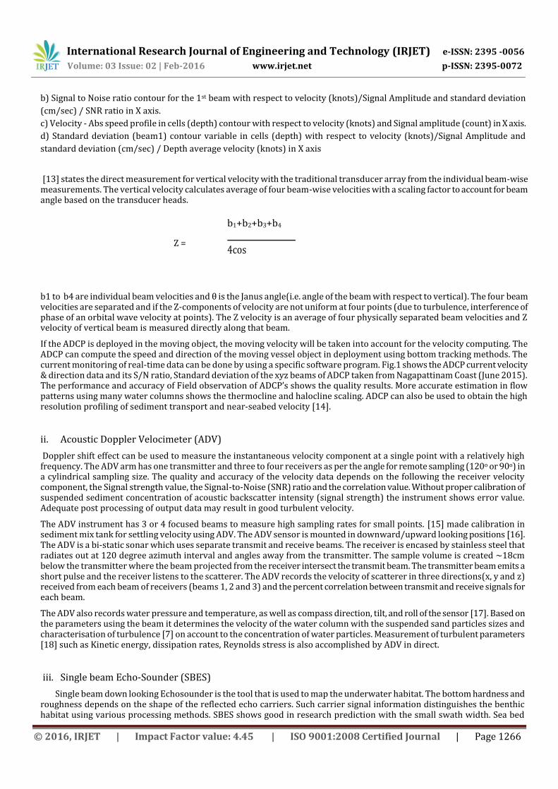
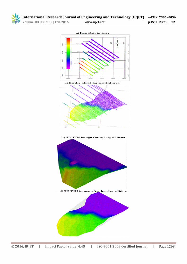
Figure 3. Single Beam Echo-Sounder for bathymetry survey applications & hydrodynamic change prediction over

the period:

a) survey lines raw data before the error correction.

b) 3D TIN (Triangulated Irregular Network) image for surveyed area after error corrections.

c) Border edited image for the confined area after heave & tide corrections.

d) 3D TIN image after the border editing

In order to characterize the shelf seafloor, the single and multi beam backscatter signal were used along with grab sediment samples. Using the clustering technique (PCA) the relationship between acoustic backscatter strength, grain size and the benthic macro-fauna are mapped. The substrate type and faunal functional groups are correlated using clustering analysis based on backscatter values. Hence by using the technique for further applications SBES in high frequency backscatter data, echo-sounding system interprets seafloor sediment and benthic habitat characteristics across large areas of seafloor. Fig. 3 shows the bathymetry contours, raw data and output processed images in TIN model of the data taken from Chennai coast (June 2015).

iv. Multibeam Echo-Sounder (MBES)

It is the most advanced tool available for remote observation and characterization of seafloor. It’s also capable of mapping seabed with fine bathymetry, to discriminate different types of seafloor habitats. By using beamforming, extraction of directional information from sound waves producing swath from a single ping of depth reading. Using multibeam echosounder, the bathymetry to map the coverage and bio-characteristics of seagrass was done already [20] and this studies limited to specific sea grass types which depends on frequency of transducer.

v. Side Scan Sonar

It is the imaging sonar or bottom classification sonar which efficiently makes the sea floor mapping in large areas. The sonar device transmits the conical shaped pulses to the seafloor in a wide angle perpendicular to the path of the sensor. The acoustic signal that is reflected from the seafloor is recorded in series which gives the sea bottom image within the swath. The sea floor is segmented in difference of material and texture types of seabed.

In addition to predicting the change in the ocean dynamics it can also be used to detect the debris, obstruction on sea floor and pipelines & cables on the floor. The shallow water structure of seabed is acquired by bathymetry sounding and sub-bottom profiling data. Fig. 4 & 5 shows the side scan echart bathymetry data with different frequency and sub-bottom profiling data in shallow water region near to Pondicherry coast (June 2015).

Figure 4. Side Scan Sonar echart scanned seafloor data of the seabed with varied frequency in different depth




Figure 5. Side Scan Sonar sub-bottom profiling echart data for different shallow water regions

Other applications such as identifying sea resources, dredging operation and environmental change prediction make use of side scan sonar. The sound frequency range is from 100 to 500kHz and to get high resolution image the higher frequency should be employed but it ranges very less.

vi. Tide Gauge

Tide gauge records the sea level changes over decades. Measurement is to be based on nearby geodetic benchmark. For research investigation the vertical crustal movement is estimated by the difference in sea level change data from tide gauge. It records the long term assessment of sea level change including meteorological factors such as barometric pressure and wind speed.

vii. Optical Laser diffraction Instrument (LISST)

LISST consists of a laser, optics, multi ring detector, signal amplifying and data scheduling circuits. It provides real time data on sediment concentration and particle size distributions. It computes fluxes for upto 32 particle size classes at points, vertical or in the entire stream cross section based on velocity and concentration. The instrument uses the laser diffraction (Mie theory) technique to obtain the particle size-distribution as well as suspended sediment concentration (SSC).

The measurement principle [21] of the LISST is that the collimated laser beam is sent through a sample volume. The particles crossing the laser beam forward the scattered light at a particular angle. With increasing radii the photo detector represents 32 small forward angles. The instrument records the scattered intensity as volume scattering functions, also by use of mathematical inversion, scattering intensity is converted into data as PSD. The photodiode placed behind the small hole in the detector makes it possible for measurement of optical transmission of laser beam. The suspended particle concentration [22] range can be measured by the instrument which is the function of particle size and path length of collimated laser beam.

The range of optical transmission is between 0.3 to 0.98 and if the optical transmission is ~40 the sample volume has less particles that states sampling volume is too clear for reliability. If the sample volume is too turbid multiple scattering effect may occur and the value is lower than 0.3. Multiple scattering refers re-scattered light in optical transmission. The laser diffraction based instrument does not measure the suspended sediment concentration directly but it measures volume concentration (VC). To measure the mass concentration volume concentration is multiplied by particle density. The different laser diffraction method [23] deliver PSD to sphere sizes in which the shape effect of grains is also included for the processing of result.




viii. Optical Backscatter point Sensor (OBS)

OBS measures the turbidity and suspended solid concentration by infra-red light scattered from suspended matters. Scattering depends on size, composition and shape of suspended particles [24]. The range of measurement for sand particles (in water free of silt and mud) is 1 to 100 kg/m3 with sampling frequency of 2 Hz. Measuring angle ranges from 140o to 165o. The detector integrates IR-light scattered between 140o to 160o. OBS calibrated response are consistent with correction made for suspended sediment size, precise time and apparent noise in records. [25] used included fluorometers, PAR irradiance sensors, Lu683 sensors, and a spectral radiometer of OBS sensors for determining annual cycle of phytoplankton biomass by transforming signals from the optical sensors into chlorophyll a (chl a).

CONCLUSION

The sensor based instruments discussed in this paper can be used for the investigation of hydrodynamics and sediment process in coastal, river mouth, estuary, onshore and offshore regions. The primary data recorded from these instruments can be used to find out ocean characteristics for analysis, processing and prediction. Highly accurate calibration is required to characterize the relationship between acoustic, optical and other properties with the sediment transport parameters. Corrections and Calibration should be done before setting the instrument in the field else the error value will be high. Given output data in figures (Fig. 1, 3, 4 & 5) should be the sample data which proves the instrument output and the accuracy of the instrument. The techniques and technology provided here proves adequate to study the features of ocean dynamics and process in the future.

REFERENCES

[1] Murali R. M., Seelam J. K., and Gaur A. S., 2014: Shoreline changes along Tamil Nadu coast : A study based on archaeological and coastal dynamics perspective, vol. 43, no. July, 2014.

[2] Wright et al. 1994: Hydrodynamic processes in the coastal zone.

[3] Kjerfve B. and Magill K., 1989: Geographic and hydrodynamic characteristics of shallow coastal lagoons, Mar. Geol., vol. 88, no. 3–4, pp. 187–199, Aug. 1989.

[4] Studies O., 2004: Air-Sea Interaction, Coastal Circulation and Primary Production in the Eastern Arabian Sea : A Review, vol. 60, pp. 205–218, 2004.

[5] Schott F. A. and J. P. M. Jr., 2001: The monsoon circulation of the Indian Ocean, vol. 51, pp. 1–123, 2001.

[6] Chauhan M. S., Kumar V., Dikshit P. K. S., and Dwivedi S. B., 2014: Comparison of Discharge Data Using ADCP and Current Meter, vol. 3, no. 2, pp. 81–86, 2014.

[7] Gratiot N., Mory M., and Auche D., 2000: An acoustic Doppler velocimeter ( ADV ) for the characterisation of turbulence in concentrated mud, vol. 20, pp. 1551–1567, 2000.

[8] Irish J. D., Hay a. E., Traykovski P., Newhall A., Craig R., and Paul W. M., 2002: On attaching acoustic imaging instrumentation to the LEO-15 observatory for sediment transport and bottom boundary layer studies, IEEE J. Ocean. Eng., vol. 27, no. 2, pp. 254–266, Apr. 2002.

[9] Storlazzi C. D., 2014: Coastal circulation and water-column properties in the War in the Pacific National Historical Park, Guam: measurements and modeling of waves, currents, temperature, salinity, and turbidity, April-August 2012.

[10] Creed E. L., Pence A. M., and Rankin K. L., 2001: Inter-comparison of turbidity and sediment concentration measurements from an ADP, an OBS-3, and a LISST, MTS/IEEE Ocean. 2001. An Ocean Odyssey. Conf. Proc. (IEEE Cat. No.01CH37295), vol. 3, pp. 1750–1754.

[11] Lacy J. R. and Sherwood C. R., 2004: Accuracy of a pulse-coherent acoustic Doppler profiler in a wave-dominated flow,” J. Atmos. Ocean. Technol., vol. 21, pp. 1448–1461, 2004.




[12] Englert C. M., Butkiewicz T., Mayer A., Schmidt V., Beaudoin J., Trembanis A. C., and Duval C., 2013: Designing Improved Sediment Transport Visualizations Binding a GIS data model with human perception research, 2013.

[13] Wanis P., 2013: Design and Applications of a Vertical Beam in Acoustic Doppler Current Profilers, 2013.

[14] Van Unen R. F. and Bosman J. J., 1996: AND SEDIMENT TRANSPORT PROFILING, pp. 483–488, 1996.

[15] Cart G. M., Friedrichs C. T., and Panetta P. D., 2012: Dual Use of a Sediment Mixing Tank for Calibrating a Acoustic Backscatter and Direct Doppler Measurement of Settling Velocity, 2012.

[16] Buschmann F., Erm A., Alari V., Listak M., Rebane J., and Toming G., 2012: Monitoring sediment transport in the coastal zone of Tallinn Bay, 2012 IEEE/OES Balt. Int. Symp., pp. 1–13, May 2012.

[17] Hatteras C., Carolina N., Martini M., Armstrong B. and Warner J. C., 2009: High resolution near-bed observations in winter near, 2009.

[18] Lohrmann A., Cabrera R., Gelfenbaum G., and Haines J., 1995: Direct measurements of Reynolds stress with an acoustic Doppler velocimeter, Proc. IEEE Fifth Work. Conf. Curr. Meas., pp. 205–210, 1995.

[19] Haris K., Chakraborty B., Ingole B., Menezes A., and Srivastava R., 2012: Seabed habitat mapping employing single and multi-beam backscatter data: A case study from the western continental shelf of India, Cont. Shelf Res., vol. 48, pp. 40–49, Oct. 2012.

[20] Komatsu T., Igarashi C., Tatsukawa K., Sultana S., Matsuoka Y. and Harada S., 2003: Use of multi-beam sonar to map seagrass beds in Otsuchi Bay on the Sanriku Coast of Japan, Aquatic Living Resources, 16 (2003), 223–230

[21] Haun S., Rüther N., Baranya S., and Guerrero M., 2015: Comparison of real time suspended sediment transport measurements in river environment by LISST instruments in stationary and moving operation mode, Flow Meas. Instrum., vol. 41, pp. 10–17, Mar. 2015.

[22] Agrawal Y.C., Mikkelsen O. A., Pottsmith H.C., 2011: Sediment monitoring technology for turbine erosion and reservoir siltation applications. In: Proceedings HYDRO 2011 conference. Prague, Czech Republic; 2011.

[23] Agrawal Y.C., Whitmire A., Mikkelsen O.A., Pottsmith H.C., 2008: Light scattering by random shaped particles and consequences on measuring suspended sediments by laser diffraction. J Geophys Res 2008:113.

[24] Deines K. L., 1999: Backscatter estimation using Broadband acoustic Doppler current profilers, in Proc. IEEE Working Conf. on Current Measurement, 1999, DOI: 10.1109/CCM.1999.755249.

[25] Kinkade C. S., Marra J., Dickey T. D., and Weller R., 2001: An annual cycle of phytoplankton biomass in the Arabian Sea, 1994–1995, as determined by moored optical sensors, Deep Sea Res. Part II Top. Stud. Oceanogr., vol. 48, no. 6–7, pp. 1285–1301, Jan. 2001.

ocean dynamics and sediment transport measuring · pdf file ·...

Documents