Observations of the BL Lac Jet Acceleration/Collimation Region

Review of Marscher et al. (2008) and Related Theoretical Papers

David Meier (JPL)

Outline

• Review of Hydrodynamics (waves, causality, wind principles)

• Introduction to Magneto-Hydrodynamics (waves, causality, jet principles)

• Self-similar jet models (cold, warm; slow, fast)

• The Marscher et al. paper (results, interpretation, and significance)

HYDRODYNAMICS

Non-dispersive HD (Sound) Waves

Adiabatic Sound Speed

Dispersion Relation for Sound Waves

HD Causality

• Any k is valid, so – Sound waves are isotropic– But they are Doppler shifted in direction of flow when V

0

• a) Subsonic Flow (V < cs): – Points A and B can both affect each other– The entire region is causally connected

• b) Supersonic Flow (V > cs):– Point A can affect point B– But, point B cannot affect point A– Information flows downstream only

• Mach Cones and Caustics– Mach cone is similar to light cone: divides the sonic past

from the sonic future– Caustic is a vector, tangent to the Mach cone, pointing

toward sonic future– Mach cones & caustics appear only when V exceeds cs

Bogovalov (1994)

HD Windsmoving

• The velocity in a single streamline in a smoothly-accelerating wind will eventually pass through the Sonic Point, where V = cs

• The full set of such streamlines creates a “Sonic Surface” (SS)• Caustics and Mach cones appear (or disappear) at sonic surfaces• In order for the flow across the sonic surface to be “regular”, an implicit

“regularity condition” must be satisfied: the numerator of the wind equation also must = 0 there, or

rs = GM/2cs2

IDEALMAGNETOHYDRODYNAMICS

Non-dispersive MHD Waves: 1. Alfven

Alfvén Velocity Vector

Full Dispersion Relation

Alfvén Dispersion Relation

transverse (Alfvén)

longitudinal (magneto-acoustic)

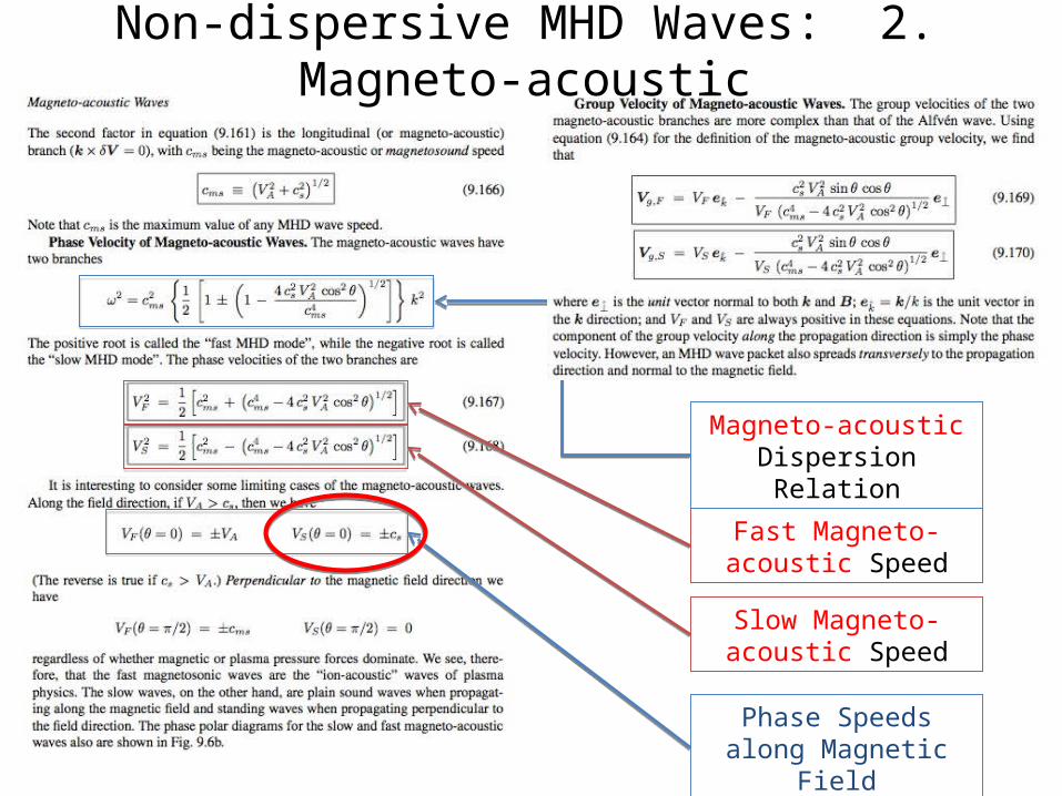
Non-dispersive MHD Waves: 2. Magneto-acoustic

Fast Magneto-acoustic Speed

Magneto-acoustic Dispersion Relation

Phase Speeds along Magnetic Field

Slow Magneto-acoustic Speed

MHD Causality• Phase velocity remarks

– Slow magneto-acoustic velocity is• cs along the magnetic field (sound wave!)• Zero normal to the magnetic field

– Fast magneto-acoustic velocity is• VA along magnetic field (but still compressive,

not Alfven) • cms = (VA

2 + cs2)1/2 normal to the magnetic field

• Group velocity remarks– Friedrich’s (polar) diagrams used to

determine caustics: • Pick fluid velocity point (magnitude & direction)• Draw tangents from branch curve to point• Sub(magneto)sonic velocities produce no

tangents, hence no caustics; flow at that speed is fully causally connected

– Special branch of the slow mode (the “cusp” wave)

• Transmits information BACKWARD• ITS caustics disappear when V < Vc = cs VA / cms

MHD Winds (Linearly Accelerating)• Assume that V || B • A linearly-accelerating MHD wind

consists of 5 regions:– V < Vc (A)– Vc < V < VS (B, C)– VS < V < VA (D)– VA < V < VF (E)– VF < V (F, G, H)

• There are three sonic surfaces where caustics appear or disappear• Cusp surface (CS)• Slow Magnetosonic Surface (SMS)• Fast Magnetosonic Surface (FMS)

• At the Alfven Surface caustics do not appear/disappear• But, they do change sign• The Alfven Surface, therefore, is a “separatrix surface”

MHD Winds (Collimating Jets)• From Bogovalov (1994)• Adding curvature (collimation) to the

MHD wind lifts the degeneracy at the SMS & FMS

• Each splits into – A magnetosonic surface and– A separatrix surface, where caustics

change direction

• Separatrix surfaces• Are physical, not mathematical, surfaces• Are generated by the causal nature of MHD• Act as initial hypersurfaces or internal boundaries• Need to have conditions specified on them that propagate throughout the entire flow

• There are, therefore, three important separatrix surfaces that determine the nature of an accelerating, collimating jet

• The Alfven Surface (AS)• The Slow Magnetosonic Separatrix Surface (SMSS)• The Fast Magnetosonic Separatrix Surface (FMSS)

• And there are still three additional and distinct sonic surfaces (CS, SMS, FMS)• However, note this important point:

• The FMS is no longer the “horizon”, where information flow is downstream only• The actual magnetosonic horizon in a collimating jet is the FMSS

CS

AXISYMETRIC, IDEALMAGNETOHYDRODYNAMICS

AXISYMMETRIC, STATIONARY, IDEAL MAGNETOHYDRODYNAMICS

• Like all conservation laws, MHD is a function of the event point in spacetime (r, θ, ϕ, t)

• Full 3-D, time-dependent simulations are the most realistic (Nakamura, Spitkovsky, McKinney, Anninos & Fragile, etc.)

• Many have performed 2-D, axisymmetric simulations (∂/∂ϕwhich still afford some realism(r, θ, t)

• Time-Independent (stationary; ∂/∂t = 0) MHD studies offer perhaps the best compromise:

– Steady-state view of a 2-D, axisymmetric system– Semi-analytic insight into large regions of parameter space

• The axisymmetric, stationary equations of ideal MHD are a special and VERY useful set and used for pulsars, jets, black holes, etc.

• They have the following properties (not derived here today) …

AXISYMMETRIC, STATIONARY, IDEAL MAGNETOHYDRODYNAMICS (cont.)

• If Ω ≠ 0, they produce rotation-driven, outflowing wind (or inflowing accretion)• Along a given magnetic field line, several physical quantities are constant:

– Angular velocity of the magnetic field line: Ω = Ωf

– The local magnetic flux in a given poloidal area: B dSp

– The local mass flux in a given poloidal area: 4π ρ γ V dSp

• This leads to an extraordinary result, independent of field strength (Chandrasekhar 1956, Mestel 1961): the poloidal magnetic field and velocity are parallel with the proportionality constant

k = 4π ρ γ Vp / Bp

• … leading to a closed form for the plasma velocity in terms of the magnetic fieldV = k B / 4π ρ γ + R Ω eϕ

• This is a special case of the “frozen-in field”: in the poloidal plane– Plasma flows along the field and– The field is carried along by the flow

• Additional quantities are conserved along B: – Angular momentum per unit mass (including field a.m.)– Total energy (Bernoulli constant)– The adiabatic coefficient KΓ

SELF-SIMILAR, AXISYMMETRIC, STATIONARY, IDEAL

MAGNETOHYDRODYNAMICS:

The MHD Jet Analogy to the Parker Wind

Thermal / Relativistic Properties

Non-Relativistiic Relativistic

Cold (p = 0) Blandford & Payne (1982)(2 singular points: AS, FMSS)

Li, Chiueh, Begelman (1992)(2 singular points)

Warm (0 < p < B2/8π) Vlahakis et al. (2000)(3 singular points: add SMSS)

Vlahakis & Konigl (2003)(3 singular points)

Table of Important Self-Similar MHD Jet Papers in the Last ¼ Century

THE SELF-SIMILAR ASSUMPTION and SELF-SIMILAR MHD JET EQUATIONS

• Removes one more degree of freedom, turning the 2-D partial differential equations into 1-D ordinary differential equations

• Possible self-similarity assumptions:– Cylindrical Z: presupposes a collimated vertical jet structure– Cylindrical R: useful for accretion disk structure, not jets– Spherical θ: similar to spherical wind (NO collimation)– Spherical r: only choice with equations that allow collimation

• Blandford & Payne (1982) chose the latter: – r-self-similarity; θ structure same for every field line– Reduces MHD to only two ordinary differential equations in θ

• Standard procedure for deriving any (MHD) wind/jet equation:– Derive the (algebraic) conservation of energy (Bernoulli) equation; then differentiate it to obtain

a1 dM / dθ + b1 dψ / dθ = c1

where M is the Alfven Mach number and ψ is the local magnetic field/velocity angle– Derive another equation that is skew, if not orthogonal, to the differentiated Bernoulli eq. (BP

used the Z-component of the momentum equation) to obtain the “cross-field” equation:a2 dM / dθ + b2 dψ / dθ = c2

– Solve for dM / dθ and dψ / dθ to get 2 coupled ordinary differential equations. For example…

dM / dθ = N / D = (c1 b2 - c2 b1 ) / (a1 b2 - a2 b1 ) – Integrate numerically w.r.t θ, applying the regularity condition N = 0 at any θ where D = 0

• Blandford & Payne’s equation was only slightly different:

• DNR = 0 at two points:– Alfven “point” (where a single field line crosses the Alfven surface): MNR = ±1 or

Vθ = ± Bθ / (4πρ)1/2 Vp = ± Bp / (4πρ)1/2

– “Modified Fast Point” (single field line crosses the Fast Magnetosonic Separatrix Surface [FMSS]) Vθ = ± B / (4πρ)1/2

– VERY IMPORTANT: The MFP occurs where the collimation speed toward the axis (Vθ) equals the fast magneto-acoustic speed!

– This can occur VERY FAR from the black hole (e.g., 104-5 rg)

THE SELF-SIMILAR ASSUMPTION and SELF-SIMILAR MHD JET EQUATIONS (cont.)

Sonic Radius

Hydrostatic Solar Wind

Supersonic Solar Wind

Sonic P

oint

Poynting Flux Dominated

What happens beyond the MFP?

RECAP SO FAR: SELF-SIMILAR JET ACCELERATION AND COLLIMATION THEORY

• After launching, jet continues to be accelerated and collimated by the rotating magnetic field

• The process is similar to the Parker solar wind

• MHD jets have 3 singular points (Blandford & Payne 1982; Vlahakis & Konigl 2004): MSP, AP, MFP

Modified Slow Point

(Vθ = Vslow)

Alfven Point (Vjet = VAlfven)

Vjet = Vfast = (VA2+cS

2)1/2 (not a singular point)

Modified Fast Point (Vθ = -Vfast)

Collimation Shock !! Kinetic Energy Flux Dominated

• Side Notes:• FR II jets appear to be Kinetic Energy Flux Dominated

Strong collimation shock disrupted jet in the nucleus at ~MFP (i.e., 104-5 rg)• Some FR I jets appear to be Poynting Flux (magnetically) Dominated

Weak or absent MFP• But, FR I sources are likely to be a very heterogeneous lot

SMSS AS FMSS

• Blandford & Payne (1982) summary:– Assumed cold plasma (p = 0), so did not have a Modified Slow Point (SMSS)– Assumed Keplerian rotation at the base of the outflow, so had a specific Ω(R) and Bϕ(R) at base– Assumed final jet was cylindrical, so there never was a true MFP either (i.e., θMFP = 0)!– I.e., the solution had only an Alfven point– Typical model results:

• Jet Total Luminosity: LT ≈ 2.4 Ψ2out Ωout / R0,max = 2.4 B2

out R30,max Ωout

• Jet Mass Loss Rate: ΔM ≈ 0.02 Ψ2out / R3

0,max Ωout = 0.02 B2out R0,max / Ωout

• Jet Torque (A.M. loss): G ≈ 0.51 Ψ2out / R0,max = 0.51 B2

out R30,max

• Li, Chiueh, & Begelman (1992) summary:– Added relativistic flow; NOTE: self-similarity assumption was NOT compatible with gravity (not

even Newtonian gravity); So, gravity is not included in relativistic self-similar MHD– Used a true cross-field equation, instead of Z-component momentum equation– Similar denominator to BP, but with relativistic expressions for Alfven and Fast speeds;

also much more complex numerator; ALSO sought cylindrical solutions and ignored the MFP– Obtained Lorentz factors up to ~ 50– Typical results similar to BP, but with R0,max replaced with RL,out; that is, scale radius is now the

LIGHT CYLINDER radius of the outermost magnetic field line• Jet Total Luminosity: LT ≈ 1.6 Ψ2

out Ωout / RL, out = 1.6 B2out R4

L, out Ω2out / c (BZ expression)

• Jet Mass Loss Rate: ΔM ≈ 0.08 Ψ2out / R3

L, out Ωout = 0.08 B2out c / Ω2

out

SELF-SIMILAR MHD JET MODELS

SELF-SIMILAR MHD JET MODELS (cont.)

• Vlahakis, Tsinganos, Sauty, & Trussoni (2000) summary:– Assumed warm plasma (0 < p < B2/8π), so did have a Modified

Slow Point (SMSS):D Vθ

4 - Vθ2 cms

2 + cs2 V2

A,θ

– Also achieved a true Modified Fast Point (FMSS)– So, the solution had all three singular points– Actually used the polar angle θ as the dependent variable, rather

than Z or R– MFP

Specific Energy vs. Z Diagram

Bogovalov-type Causality

Diagram for MHD Jet Model

SELF-SIMILAR MHD JET MODELS (cont.)

• Vlahakis & Konigl(2003,2004) summary:– Can be considered to be a combination of Li et al. (1992) and Vlahakis et al. (2000):

relativistic AND warm flow, with MSP and MFP– These are the models to use for AGN, microquasars, etc.

Model for 3C 345: Specific Energy and

Velocity Components vs. R Diagrams

γ≈

SELF-SIMILAR MHD JET MODELS: SUMMARY• Basic Model:

– Three separatrix surfaces (manifested as modified singular surfaces in the equations)– Three sonic surfaces (cusp, classical slow, classical fast)

Poynting Flux Dominated

What happens beyond the MFP?

Alfven Point (Vjet = VAlfven)

Vjet = Vfast = (VA2+cS

2)1/2 (not a singular point)

Modified Fast Point (Vθ = -Vfast)

Collimation Shock !! Kinetic Energy Flux DominatedSMSS

(SMP)AS

(AP)FMSS (MFP)

• What happens after the MFP is a mystery; at least 2 possibilities:– Convergence creates a strong collimation shock, converting magnetic energy to particle energy

and jet to kinetically dominated– Flow remains magnetically dominated (bounce instead of shock)

Poynting Flux Dominated

OBSERVING THE JET ACCELERATION & COLLIMATION

REGION

• Is the MHD model at all viable? – Can we detect a helical, well-ordered magnetic field in this region?– Is there any evidence of rapid rotation of the jet plasma or features?

• Where does the gamma-ray emission come from? Shocks? Emission deep in the collimation or launching region?

• What happens at the MFP and beyond?– Does a strong, field-destroying shock develop?– Or is there a gentler transition, leaving the jet still in a Poynting flux/magnetically-dominated

state?– Does this answer depend on the type of source (e.g., FR I, FR II)

• NOTES:– FR I jets are expected to collimate slowly collimation regions 103-5 rg in length or more

• M87 1.4 – 140 mas in size• Cen A 0.6 – 60 mas in size• BL Lac 0.006 – 0.6 mas in size (foreshortened)

– FR II jets are expected to collimate quickly collimation regions 10 - 100 rg in length, AND BE FARTHER AWAY

• Cyg A 1 – 10 μas in size• 3C 35 0.4 – 4 mas in size

QUESTIONS TO TRY TO ANSWER WITH OBSERVATIONS

• Observed BL Lac with VLBA, UMRAO/Metsahovi, Steward/Crimea, XTE, & ?? (TeV)• 2 γ-ray flares (~2005.82, 2005.88) detected• Outbursts also seen in radio, optical (R-band), & X-ray during γ-ray flaring period• Particularly important results:

– γ-ray flaring period occurs during the birth of a new VLBI component– First γ-ray flare occurs simultaneously with a 240 degree polarization rotation in the optical– Optical polarization reaches 15% VERY strong magnetic field– Unfortunately, 2nd γ-ray flare has no optical polarization data

MARSCHER et al. (2008, Nature, 452, 966)

2005.82 2005.88

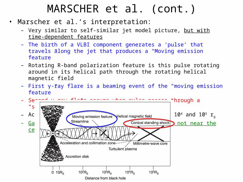
• Marscher et al.’s interpretation:– Very similar to self-similar jet model picture, but with time-dependent features– The birth of a VLBI component generates a ‘pulse’ that travels along the jet that produces a

“Moving emission feature”– Rotating R-band polarization feature is this pulse rotating around in its helical path through

the rotating helical magnetic field– First γ-ray flare is a beaming event of the “moving emission feature”– Second γ-ray flare occurs when pulse passes through a “standing shock”– Acceleration & collimation region is between 104 and 105 rg

– Gamma-rays are produced by shocks in the jet, not near the central engine

MARSCHER et al. (cont.)

• My additions:– The “moving emission feature” is actually an MHD slow-mode shock, which is constrained

to travel ONLY along the helical magnetic field (recall properties of slow-mode waves)– The coherent 240 degree polarization swing is strong evidence for a well-ordered helical

magnetic field; knowing the “beaming angle” we could calculate the field pitch angle– The “standing shock” is probably a collimation shock produced near the MFP, and

represents the place where the jet nozzle ends and free jet flow begins– However, the lack of polarization data during and after 2nd flare is a severe loss– We cannot tell whether plasma is strongly magnetized or becomes turbulent and,

therefore, cannot tell for certain whether a true MFP exists or not– BL Lac’s parent is probably an FR I; FR II objects are likely to be quite different

MARSCHER et al. (cont.)

They don’t know this to be the case!!

• Importance and significance of the Marscher et al. (and future such) observations– First time we have peered into the “central jet engine” and seen a little bit of how it works

– This is the ONLY method we have (probably for decades) to probe the acceleration & collimation region of ANY ASTROPHYSICAL JET (AGN, protostellar, microquasar, symbiotic, GRB, SN, nor PN)

– The high-resolution imaging of the VLBA is essential for determining the location of optical/X-/γ-ray features

– Multi-wavelength observations, esp. optical & hard X-/γ-ray are essential for probing the internal structure of the jet

– Space VLBI will provide even higher resolution, allowing perhaps a probe of an FR II-class object

– One of the most important mysteries to solve is why are FR II sources so kinetically dominated, if all jets are magnetically accelerated and collimated?

– Where is the magnetic energy converted into non-thermal internal energy? (In the MHD model it’s converted into kinetic energy in the acceleration/collimation region.

– Our old, bright VLBI source friends are probably the best candidates for this type of work: • They are bright, giving very good S/N• We are peering down jet engine nozzle• Helical field easily identified with multi-frequency polarization observations• They evolve on relatively short time scales

• All we need is the highest angular VLBI resolution and best (u,v)-coverage possible

MARSCHER et al. (cont.)