object recognition using moments of the signature
TRANSCRIPT
OBJECT RECOGNITION USING MOMENTS
OF THE SIGNATURE HISTOGRAM
by
Dustin G. Coker, B.S., B.A.
A thesis submitted to the Graduate Council of Texas State University in partial fulfillment
of the requirements for the degree of Master of Science
with a Major in Computer Science May 2017
Committee Members:
Dan E. Tamir, Chair
Byron Gao
Yijuan Lu

COPYRIGHT
by
Dustin G. Coker
2017

FAIR USE AND AUTHOR’S PERMISSION STATEMENT
Fair Use
This work is protected by the Copyright Laws of the United States (Public Law 94-553, section 107). Consistent with fair use as defined in the Copyright Laws, brief quotations from this material are allowed with proper acknowledgement. Use of this material for financial gain without the author’s express written permission is not allowed.
Duplication Permission
As the copyright holder of this work I, Dustin G. Coker, authorize duplication of this work, in whole or in part, for educational or scholarly purposes only.

iv
ACKNOWLEDGEMENTS
I would first like to acknowledge my thesis advisor Dr. Dan Tamir for his assistance in completing this work. His support and guidance have been remarkable. I cannot thank him enough for his patience and especially his good humor during this process. His commitment to helping students is an inspiration and I am eternally grateful for everything he has done for me personally. I'd also like to thank Dr. Byron Gao. I am extremely thankful for not only his participation as a member of my thesis committee but also for his help and guidance during my initial graduate work. I thank Dr. Yijuan Lu for participating as a member of my thesis committee and her helpful suggestions and instruction. Finally, I would also like to thank my family, especially my wife, Nova. I could not have done this without her support and sacrifice. She is the light of my life and my best friend. My daughters, Zoey and Scarlet, have been my inspiration. Their laughter is medicine. My girls are my everything. Thank you.

v
TABLE OF CONTENTS
Page
ACKNOWLEDGEMENTS ......................................................................................... iv
LIST OF TABLES .................................................................................................... viii
LIST OF FIGURES ..................................................................................................... ix
ABSTRACT .................................................................................................................. x
CHAPTER
I. INTRODUCTION ............................................................................................... 1
II. BACKGROUND ................................................................................................ 4
2.1 Image Processing ........................................................................................ 4
2.1.1 Images ................................................................................................ 4
2.1.2 Neighbors ........................................................................................... 5
2.1.3 Digital Path ........................................................................................ 6
2.1.4 Connectivity ....................................................................................... 6
2.1.5 Region ................................................................................................ 6
2.1.6 Contour .............................................................................................. 7
2.1.7 Descriptor ........................................................................................... 7
2.1.8 Segmentation...................................................................................... 7
2.1.8.1 Image Thresholding .................................................................. 8
2.1.8.2 Clustering-based Segmentation ................................................ 8
vi
2.1.9 Connected Component Labeling........................................................ 9
2.2 Histogram .................................................................................................. 10
2.3 Object Signature........................................................................................ 13
2.3.1 Acquiring the Object Signature ....................................................... 14
2.4 Moments ................................................................................................... 15
2.4.1 Geometric Moments......................................................................... 15
2.4.1.1 Hu's Moment Invariants.......................................................... 17
2.4.2 Contour Moments ............................................................................ 18
2.4.3 Raw Moments of the Object Signature ............................................ 20
2.4.4 Moments of a Random Variable ...................................................... 24
2.4.4.1 Normalized Moments of a Random Variable ........................ 25
2.4.5 Histogram Moments......................................................................... 26
2.4.5.1 Histogram Moment Descriptors.............................................. 26
2.5 Fourier Descriptors ................................................................................... 27
2.6 Mean Square Error .................................................................................... 30
2.7 Confusion Matrix ...................................................................................... 30
2.8 Star-Convex .............................................................................................. 31
III. RELATED WORK ......................................................................................... 32
IV. EXPERIMENTAL SETUP ............................................................................ 35
4.1 Software .................................................................................................... 35
4.2 Hardware ................................................................................................... 35

vii
4.3 Dataset ...................................................................................................... 36
4.4 Descriptors ................................................................................................ 39
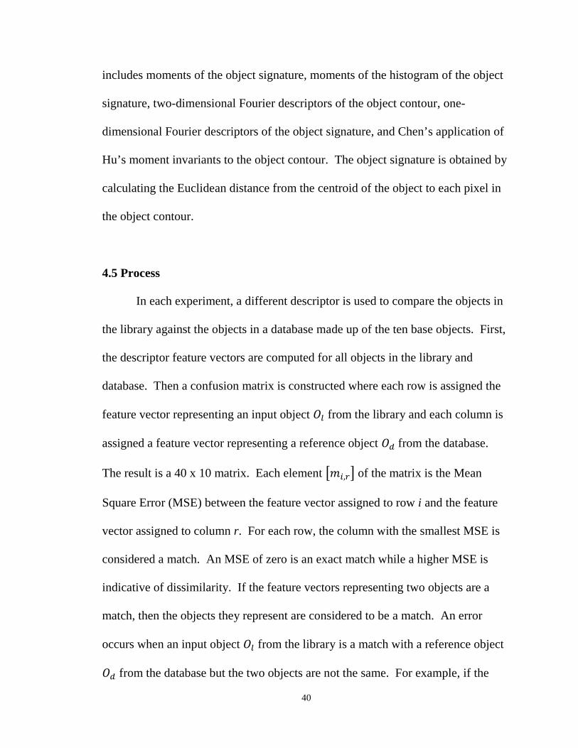
4.5 Process ...................................................................................................... 40
4.6 Comparison ............................................................................................... 41
V. EXPERIMENTS AND RESULTS .................................................................. 43
VI. RESULTS EVALUATION ............................................................................ 51
BIBLIOGRAPHY....................................................................................................... 56
viii
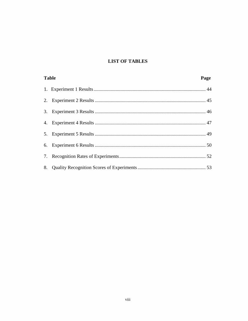
LIST OF TABLES Table Page 1. Experiment 1 Results ............................................................................................ 44 2. Experiment 2 Results ........................................................................................... 45 3. Experiment 3 Results ........................................................................................... 46 4. Experiment 4 Results ........................................................................................... 47 5. Experiment 5 Results ........................................................................................... 49 6. Experiment 6 Results ........................................................................................... 50 7. Recognition Rates of Experiments ....................................................................... 52 8. Quality Recognition Scores of Experiments ........................................................ 53

ix
LIST OF FIGURES Figure Page 1. 4-Neighbor and 8-Neighbor Sets ............................................................................ 5 2. Example Frequency Histogram ............................................................................ 11 3. Equal Angle Object Signatures for Circle and Square ......................................... 14 4. K-Point Digital Boundary in the xy-plane ........................................................... 28 5. Circle .................................................................................................................... 37 6. Ellipse ................................................................................................................... 37 7. Square ................................................................................................................... 37 8. Rectangle .............................................................................................................. 37 9. Arrow ................................................................................................................... 38 10. 8 Point Star-Convex ............................................................................................. 38 11. 16 Point Star-Convex ........................................................................................... 38 12. 29 Point Star-Convex ........................................................................................... 39 13. 37 Point Star-Convex ........................................................................................... 39 14. 45 Point Star-Convex ........................................................................................... 39
x
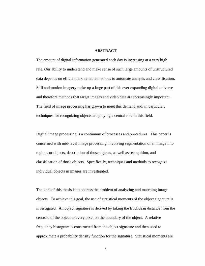
ABSTRACT
The amount of digital information generated each day is increasing at a very high
rate. Our ability to understand and make sense of such large amounts of unstructured
data depends on efficient and reliable methods to automate analysis and classification.
Still and motion imagery make up a large part of this ever expanding digital universe
and therefore methods that target images and video data are increasingly important.
The field of image processing has grown to meet this demand and, in particular,
techniques for recognizing objects are playing a central role in this field.
Digital image processing is a continuum of processes and procedures. This paper is
concerned with mid-level image processing, involving segmentation of an image into
regions or objects, description of those objects, as well as recognition, and
classification of those objects. Specifically, techniques and methods to recognize
individual objects in images are investigated.
The goal of this thesis is to address the problem of analyzing and matching image
objects. To achieve this goal, the use of statistical moments of the object signature is
investigated. An object signature is derived by taking the Euclidean distance from the
centroid of the object to every pixel on the boundary of the object. A relative
frequency histogram is constructed from the object signature and then used to
approximate a probability density function for the signature. Statistical moments are
xi
then applied to the histogram to generate a novel set of descriptors that are invariant
to rotation, translation, and scaling.
Existing techniques that utilize moments of the entire image are examined along with
moments applied to just the object contour. Additionally, the use of two-dimensional
Fourier Descriptors applied to the object contour are considered as well as one-
dimensional Fourier Descriptors applied to the object signature. Finally, moments
applied directly to the object signature are investigated. Experiments are performed
to evaluate and compare these techniques with the method introduced in this work.
Recognition accuracy as well as the quality of recognition are used to differentiate
between the various techniques.
The results of the experiments show the method introduced in this work, statistical
moments of the histogram of the object signature, proves to be a viable alternative to
the other methods discussed. In particular, since only the center bin-values of the
constructed histogram are used to calculate moments, the computational costs are
orders of magnitude smaller than the computational cost of other methods considered
in this thesis. In addition, the effect of binning the data when constructing the
histogram compensates for noise introduced by scaling and rotation, resulting in an
improvement in the quality of recognition over several of the other methods
investigated.
1
I. INTRODUCTION
The International Data Corporation estimates that by 2020, 40 zettabytes of
digital information will have been generated. With the increasing use of
connected smart devices, embedded systems, and sensors, it is expected that most
of that information will be in the form of unstructured data, such as video and
images. Consequently, there is an ever-growing need to automate the analysis of
this type of data, i.e. still and motion imagery. The use of computers to extract
meaningful information from images and video is indispensable as we try to
understand our digital universe.
The types of digital images generated today, range from electron
microscopy of bacteria to “selfies” posted on Facebook. They span an enormously
large range of the electromagnetic spectrum, from gamma rays to radio waves, and
processing these images involves different techniques and methods. The science
of Digital Image Processing has grown to meet this demand. This paper focuses
on methods to describe the constituent parts or objects of an image in a way that
facilitates recognition and differentiation between them. A good example of this
process is the modern toll road. Many newer toll roads no longer employ
tollbooths but rather use cameras to take pictures of license plates. The individual
letters and numbers of the license plate are identified and a bill sent to the
registered owner.
2
This thesis addresses the problem of analyzing and matching objects in
images. The proposed solution is to use moments of the histogram of the object
signature. Six experiments are performed. The first experiment considers a set of
seven moment-invariant descriptors. The application of those descriptors to just
the object contour is then examined. Next, the use of two-dimensional Fourier
descriptors applied to the object contour and one-dimensional Fourier descriptors
applied to the object signature is investigated. The use of mathematical moments
to describe the object signature is considered and finally, taking moments of the
histogram of the object signature is examined. The accuracy of each method in
recognizing image objects is compared along with the quality of that recognition.
The hypothesis of this thesis is that taking moments of the histogram of the
object signature is more efficient and more accurate than the other methods
discussed for object recognition.
The contribution of this research is a novel method for recognizing objects
in images. The method utilizes a minimum number of moments of the histogram
of the object signature, and due to the fact that only the center bin-values of the
histogram are used in calculating the moments, the number of computations
required are orders of magnitude smaller, resulting in effective, accurate
descriptors. Whereas other authors have applied moments to the entire image or
directly to the contour or the object signature, no one has investigated applying
moments to the histogram of the object signature.

3
This paper is organized as follows: Chapter 2 gives an introduction to
Digital Image Processing concepts and provides the necessary background for this
research. The object signature is defined along with histogram, mathematical
moments, and Fourier descriptors. Chapter 3 is a literature survey that describes
the relevant research. Chapter 4 outlines the experimental setup used to compare
and evaluate the various methods and techniques for object recognition. Chapter 5
includes the results of the experiments and in Chapter 6 the results are analyzed.
Chapter 7 presents a conclusion of our efforts and highlights future research.
4
II. BACKGROUND
2.1 Image Processing
Digital image processing is a continuum of processes and procedures.
Lower level procedures are concerned with primitive operations designed for
preprocessing the image. Mid-level image processing involves segmentation of an
image into regions or objects, description of those objects, recognition, and
classification of individual objects. At the highest level, processing consists of
interpretation of recognized objects [1]. This paper is concerned with mid-level
processing, specifically techniques and methods to recognize individual objects in
a segmented image.
2.1.1 Images
An image is represented by a two-variable function, , where x and y
are coordinates in the Cartesian plane. This function defines the intensity, or grey-
level, of the image at any pair of coordinates as follows:
𝐼𝐼 = 𝑓𝑓(𝑥𝑥, 𝑦𝑦) (1)
If the quantities x, y, and I are all discrete, the image is a digital image. A digital
image is composed of a finite number of picture elements, or pixels, each with
f x y( , )

5
discrete location (x, y) and discrete intensity I. In a binary image, the pixels only
take on one of two values, for example zero or one [1]. In this thesis, only binary
images are considered.
2.1.2 Neighbors
For pixels with coordinates (x, y), the set of 4-neighbors is defined to be the
set of pixels with coordinates
{(𝑥𝑥 − 1,𝑦𝑦), (𝑥𝑥 + 1,𝑦𝑦), (𝑥𝑥,𝑦𝑦 + 1), (𝑥𝑥,𝑦𝑦 − 1)} (2)
The set of 8-neighbors is the union of the 4-neighbors set with the set of pixels that
have the following coordinates
{(𝑥𝑥 − 1,𝑦𝑦 − 1), (𝑥𝑥 + 1,𝑦𝑦 − 1), (𝑥𝑥 + 1,𝑦𝑦 + 1), (𝑥𝑥 + 1,𝑦𝑦 + 1)} (3)
Figure 1 shows examples of 4-neighbor and 8-neighbor pixels.
Figure 1: 4-Neighbor and 8-Neighbor Sets
6
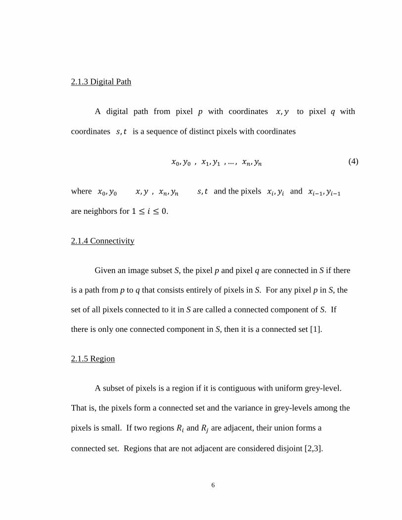
2.1.3 Digital Path
A digital path from pixel p with coordinates (𝑥𝑥, 𝑦𝑦) to pixel 𝑞𝑞 with
coordinates (𝑠𝑠, 𝑡𝑡) is a sequence of distinct pixels with coordinates
[(𝑥𝑥0, 𝑦𝑦0), (𝑥𝑥1,𝑦𝑦1), … , (𝑥𝑥𝑛𝑛, 𝑦𝑦𝑛𝑛)] (4)
where (𝑥𝑥0,𝑦𝑦0) = (𝑥𝑥,𝑦𝑦), (𝑥𝑥𝑛𝑛,𝑦𝑦𝑛𝑛) = (𝑠𝑠, 𝑡𝑡) and the pixels (𝑥𝑥𝑖𝑖 , 𝑦𝑦𝑖𝑖) and (𝑥𝑥𝑖𝑖−1,𝑦𝑦𝑖𝑖−1)
are neighbors for 1 ≤ 𝑖𝑖 ≤ 0.
2.1.4 Connectivity
Given an image subset S, the pixel p and pixel q are connected in S if there
is a path from p to q that consists entirely of pixels in S. For any pixel p in S, the
set of all pixels connected to it in S are called a connected component of S. If
there is only one connected component in S, then it is a connected set [1].
2.1.5 Region
A subset of pixels is a region if it is contiguous with uniform grey-level.
That is, the pixels form a connected set and the variance in grey-levels among the
pixels is small. If two regions 𝑅𝑅𝑖𝑖 and 𝑅𝑅𝑗𝑗 are adjacent, their union forms a
connected set. Regions that are not adjacent are considered disjoint [2,3].
7
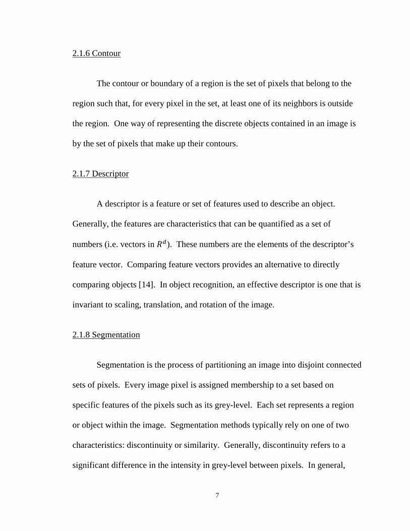
2.1.6 Contour
The contour or boundary of a region is the set of pixels that belong to the
region such that, for every pixel in the set, at least one of its neighbors is outside
the region. One way of representing the discrete objects contained in an image is
by the set of pixels that make up their contours.
2.1.7 Descriptor
A descriptor is a feature or set of features used to describe an object.
Generally, the features are characteristics that can be quantified as a set of
numbers (i.e. vectors in 𝑅𝑅𝑑𝑑). These numbers are the elements of the descriptor’s
feature vector. Comparing feature vectors provides an alternative to directly
comparing objects [14]. In object recognition, an effective descriptor is one that is
invariant to scaling, translation, and rotation of the image.
2.1.8 Segmentation
Segmentation is the process of partitioning an image into disjoint connected
sets of pixels. Every image pixel is assigned membership to a set based on
specific features of the pixels such as its grey-level. Each set represents a region
or object within the image. Segmentation methods typically rely on one of two
characteristics: discontinuity or similarity. Generally, discontinuity refers to a
significant difference in the intensity in grey-level between pixels. In general,
8
similarity refers to low variance in grey-level. Two commonly used methods for
segmentation are image thresholding and clustering.
2.1.8.1 Image Thresholding
In image thresholding, pixels with a grey-level above a specific value are
considered pixels of interest and assigned a value of 1. All other pixels are
considered background pixels and assigned a value of 0. The result is a binary
image. Methods for determining the threshold value can be classified into two
groups: global thresholding and local thresholding. Global thresholding chooses
one value that is applied to the entire image. Analysis of the shape of the image
histogram is used to determine the specific threshold value. Local thresholding
considers the neighbors of each pixel to determine the threshold for that specific
value.
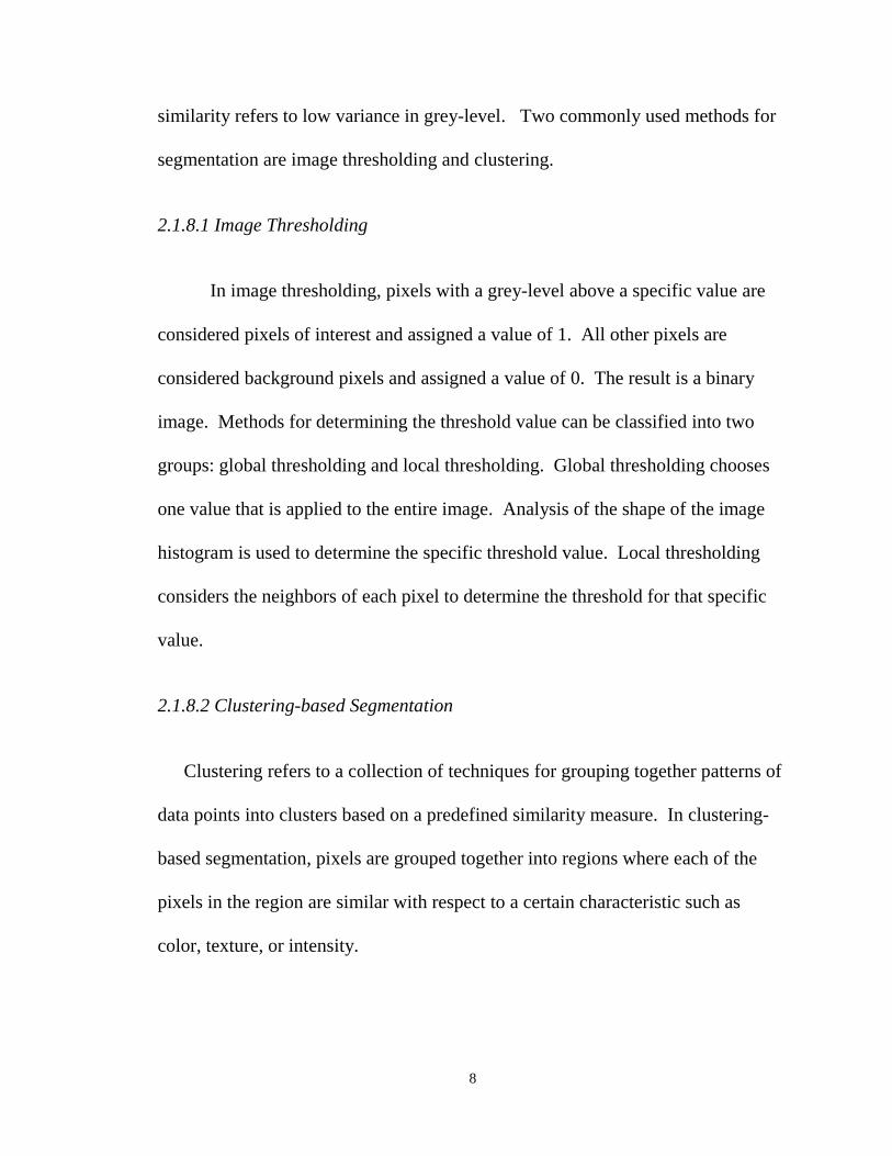
2.1.8.2 Clustering-based Segmentation
Clustering refers to a collection of techniques for grouping together patterns of
data points into clusters based on a predefined similarity measure. In clustering-
based segmentation, pixels are grouped together into regions where each of the
pixels in the region are similar with respect to a certain characteristic such as
color, texture, or intensity.

9
One example of clustering algorithms is the K-means algorithm. It takes the
input parameter, k, and partitions a set of n objects into k clusters so the resulting
intra-cluster similarity is high but the inter-cluster similarity is low. Cluster
similarity is measured in regard to the mean value of the objects in a cluster, which
can be viewed as the cluster’s centroid [15]. Within the context of image
processing, the algorithm is as follows
1. Pick k cluster centers, either randomly or based on some heuristic
2. Assign each pixel in the image to the cluster that minimizes the Euclidean
distance between the pixel and the cluster center
3. Re-compute the cluster centers
4. Repeat steps 2 and 3 until no more changes occur or a maximum number of
iterations is exceeded.
2.1.9 Connected Component Labeling
Connected Component Labeling (CCL) involves grouping image pixels
into subsets of connected pixels. The goal of CCL is to find all the connected
components of an image and mark each with a distinctive label.
10
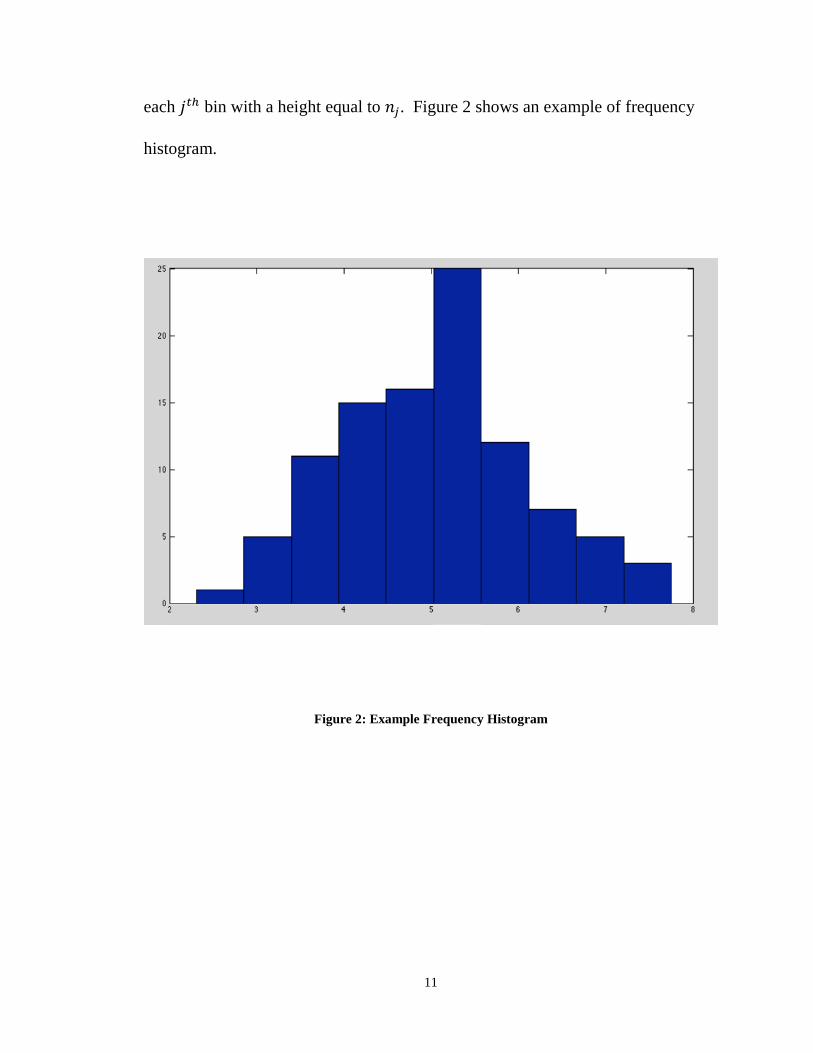
2.2 Histogram
A frequency distribution is a function showing the number of times a
variable takes on a value for each possible value. A frequency histogram is a
graphical representation of a frequency distribution. The histogram is constructed
by first dividing or binning the range of variables into intervals. A rectangle is
placed over each interval with a height equal to the number of times a variable
takes on a value that falls within that interval. For example, given a finite set of n
data points [𝑧𝑧1, 𝑧𝑧2,⋯ , 𝑧𝑧𝑛𝑛] where each 𝑧𝑧𝑖𝑖 represents an independent measurement,
it is possible to define an interval 𝐿𝐿 = [𝑎𝑎, 𝑏𝑏] such that
𝑎𝑎 < 𝑚𝑚𝑖𝑖𝑚𝑚 𝑧𝑧𝑖𝑖 < max 𝑧𝑧𝑖𝑖 < 𝑏𝑏 (5)
The interval L can then be divided into m number of disjoint sub-intervals, or
“bins”, each of width
𝑤𝑤 = (𝑏𝑏 − 𝑎𝑎)/𝑚𝑚 (6)
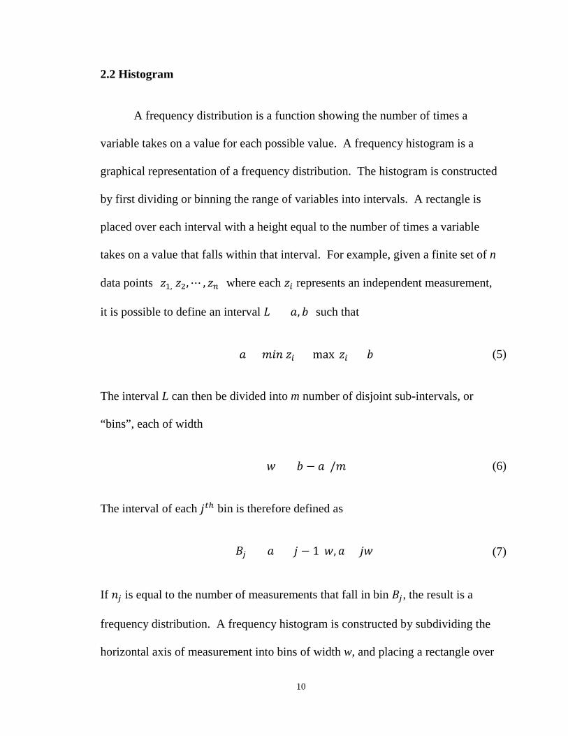
The interval of each 𝑗𝑗𝑡𝑡ℎ bin is therefore defined as
𝐵𝐵𝑗𝑗 = (𝑎𝑎 + (𝑗𝑗 − 1)𝑤𝑤,𝑎𝑎 + 𝑗𝑗𝑤𝑤] (7)
If 𝑚𝑚𝑗𝑗 is equal to the number of measurements that fall in bin 𝐵𝐵𝑗𝑗, the result is a
frequency distribution. A frequency histogram is constructed by subdividing the
horizontal axis of measurement into bins of width w, and placing a rectangle over
11
each 𝑗𝑗𝑡𝑡ℎ bin with a height equal to 𝑚𝑚𝑗𝑗. Figure 2 shows an example of frequency
histogram.
Figure 2: Example Frequency Histogram
12
The percentage of total measurements in each bin is shown by replacing 𝑚𝑚𝑗𝑗
with 𝑝𝑝𝑗𝑗 = 𝑚𝑚𝑗𝑗 𝑚𝑚⁄ . The result is a relative frequency histogram that shows the
percentage of total measurements in each bin. A relative frequency histogram
differs from a frequency histogram only in that the rectangle over each 𝑗𝑗𝑡𝑡ℎ bin
must have a height equal to 𝑝𝑝𝑗𝑗.
The probability density function (PDF) is a function that gives the
probability that a particular measurement has a certain value. A discrete random
variable is a variable that can assume only finite (or countably infinite) number of
values [8]. Using those two concepts, the relative frequency histogram can be
used to estimate the PDF for a set of measurements. If the center value for the 𝑗𝑗𝑡𝑡ℎ
bin is defined as follows
𝑣𝑣𝑗𝑗 = (𝐵𝐵𝑗𝑗+1 − 𝐵𝐵𝑗𝑗) 2⁄ (8)
then the center values of the bins can be considered to be a discrete random
variable. It is then possible to define the probability for each bin as follows
𝑝𝑝�𝑣𝑣𝑗𝑗� = 𝑚𝑚𝑗𝑗 𝑚𝑚⁄ = 𝑝𝑝𝑗𝑗 (9)
and therefore the sum of probabilities is equal to one
�𝑝𝑝𝑗𝑗 = 1𝑗𝑗
(10)
13
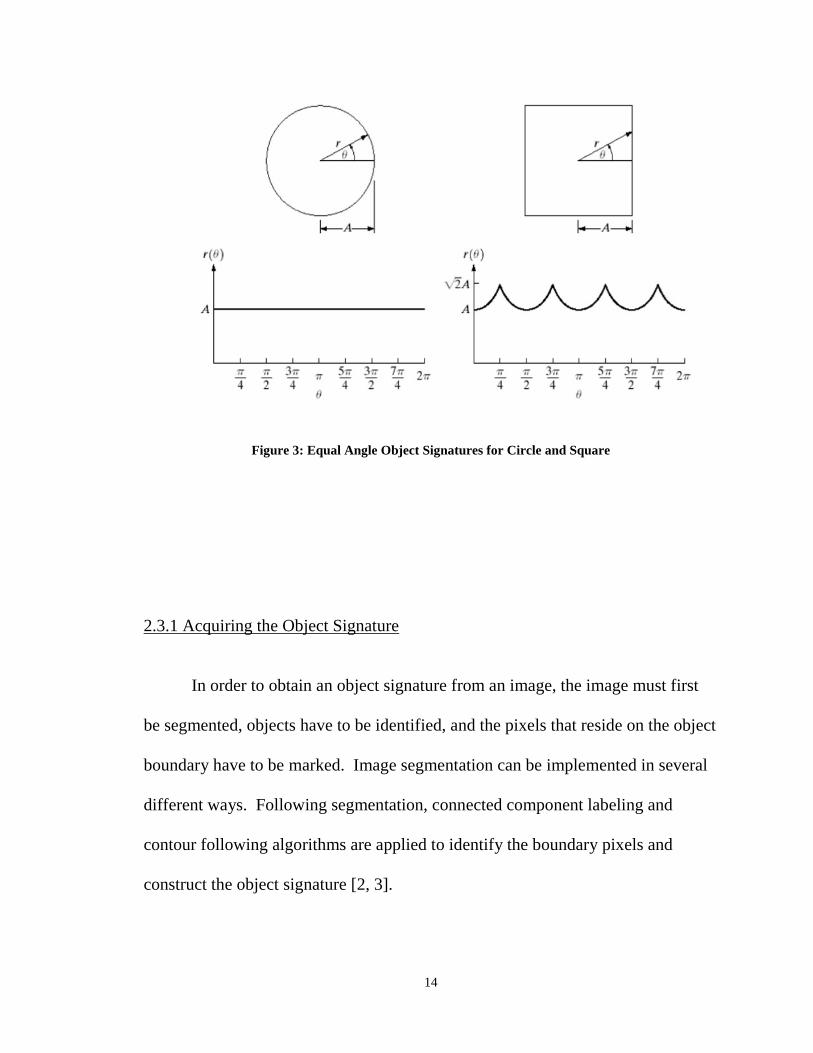
2.3 Object Signature
An object signature represents the object by a one-dimensional function
derived from object boundary points. A set of distances from a reference point to
the boundary pixels is generated. The reference point is generally the object
centroid and the distance can be measured at equal angles, or using every pixel in
the boundary. In addition to other requirements, the equal angle methods require
the object to be convex; otherwise the same angle may yield more than one
distance to the boundary. Using every pixel generates a variable number of
samples, which depends on the object. Figure 3 shows the object signature of a
circle and square respectively using the equal angle method.
14
Figure 3: Equal Angle Object Signatures for Circle and Square
2.3.1 Acquiring the Object Signature
In order to obtain an object signature from an image, the image must first
be segmented, objects have to be identified, and the pixels that reside on the object
boundary have to be marked. Image segmentation can be implemented in several
different ways. Following segmentation, connected component labeling and
contour following algorithms are applied to identify the boundary pixels and
construct the object signature [2, 3].
15
2.4 Moments
In statistics, moments are a meaningful, numerical description of the
distribution of random variables. In physics, they are used to measure the mass
distribution of a body. Both interpretations are widely used to describe the
geometric shapes of different objects.
2.4.1 Geometric Moments
Given a two-dimensional, continuous image 𝑓𝑓(𝑥𝑥, 𝑦𝑦), the geometric moment
of order (p + q) is defined as
𝑚𝑚𝑝𝑝𝑝𝑝 = � � 𝑥𝑥𝑝𝑝𝑦𝑦𝑝𝑝𝑓𝑓(𝑥𝑥,𝑦𝑦) 𝑑𝑑𝑥𝑥 𝑑𝑑𝑦𝑦
+∞
−∞
+∞
−∞ (11)
for p, q = 0, 1, 2, ….
The 𝑧𝑧𝑧𝑧𝑧𝑧𝑧𝑧𝑡𝑡ℎ order moment
𝑚𝑚00 = � � 𝑓𝑓(𝑥𝑥,𝑦𝑦) 𝑑𝑑𝑥𝑥 𝑑𝑑𝑦𝑦
+∞
−∞
+∞
−∞ (12)
represents the total mass of the image. In the case of a segmented object, the
𝑧𝑧𝑧𝑧𝑧𝑧𝑧𝑧𝑡𝑡ℎ moment of the object is the total object area [10].
The central moments are defined as
16
𝜇𝜇𝑝𝑝𝑝𝑝 = � � (𝑥𝑥 − 𝑥𝑥)𝑝𝑝(𝑦𝑦 − 𝑦𝑦)𝑝𝑝𝑓𝑓(𝑥𝑥,𝑦𝑦) 𝑑𝑑𝑥𝑥 𝑑𝑑𝑦𝑦
+∞
−∞
+∞
−∞ (13)
where
𝑥𝑥 =𝑚𝑚10
𝑚𝑚00 ,𝑦𝑦 =
𝑚𝑚01
𝑚𝑚00 (14)
After scaling equation (13) by a factor 𝛼𝛼, the central moments are expressed as
𝜇𝜇𝑝𝑝𝑝𝑝′ = � � (𝑥𝑥′ − 𝑥𝑥′)𝑝𝑝(𝑦𝑦′ − 𝑦𝑦′)𝑝𝑝𝑓𝑓′(𝑥𝑥′,𝑦𝑦′)𝑑𝑑𝑥𝑥′ 𝑑𝑑𝑦𝑦′
+∞
−∞
+∞
−∞=
= � � 𝛼𝛼𝑝𝑝(𝑥𝑥 − 𝑥𝑥)𝑝𝑝𝛼𝛼𝑝𝑝(𝑦𝑦 − 𝑦𝑦)𝑝𝑝𝑓𝑓(𝑥𝑥,𝑦𝑦)𝛼𝛼2 𝑑𝑑𝑥𝑥 𝑑𝑑𝑦𝑦+∞
−∞
+∞
−∞= 𝛼𝛼𝑝𝑝+𝑝𝑝+2𝜇𝜇𝑝𝑝𝑝𝑝
(15)
Therefore, scale invariance is achieved by normalizing each moment as follows
𝜂𝜂𝑝𝑝𝑝𝑝 =𝜇𝜇𝑝𝑝𝑝𝑝𝜇𝜇00𝛾𝛾
(16)
where
𝛾𝛾 =𝑝𝑝 + 𝑞𝑞
2+ 1 (17)
If 𝑓𝑓(𝑥𝑥,𝑦𝑦) is a digital image, the integrals are replaced with summations
17
𝑚𝑚𝑝𝑝𝑝𝑝 = ��𝑥𝑥𝑝𝑝𝑦𝑦𝑝𝑝𝑓𝑓(𝑥𝑥,𝑦𝑦)𝑦𝑦𝑥𝑥
(18)
The central moments are expressed as
𝜇𝜇𝑝𝑝𝑝𝑝 = ��(𝑥𝑥 − �̅�𝑥)𝑝𝑝(𝑦𝑦 − 𝑦𝑦�)𝑝𝑝𝑓𝑓(𝑥𝑥, 𝑦𝑦)𝑦𝑦𝑥𝑥
(19)
2.4.1.1 Hu’s Moment Invariants
Developed by Hu in 1962 [7], the following set of moments is invariant to
rotation, translation and scaling
𝜙𝜙1 = 𝜂𝜂20 + 𝜂𝜂02 (20)
𝜙𝜙2 = (𝜂𝜂20 − 𝜂𝜂02)2 + 4𝜂𝜂112 (21)
𝜙𝜙3 = (𝜂𝜂30 − 3𝜂𝜂12)2 + (3𝜂𝜂21 − 𝜂𝜂03)2 (22)
𝜙𝜙4 = (𝜂𝜂30 + 𝜂𝜂12)2 + (𝜂𝜂21 + 𝜂𝜂03)2 (23)
𝜙𝜙5 = (𝜂𝜂30 − 3𝜂𝜂12)(𝜂𝜂30 + 𝜂𝜂12)[(𝜂𝜂30 + 𝜂𝜂12)2 − 3(𝜂𝜂21 + 𝜂𝜂03)2]
+ (3𝜂𝜂21 − 𝜂𝜂03)(𝜂𝜂21 + 𝜂𝜂03)[3(𝜂𝜂30 + 𝜂𝜂12)2
− (𝜂𝜂21 + 𝜂𝜂03)2]
(24)
18
𝜙𝜙6 = (𝜂𝜂20 − 𝜂𝜂02)[(𝜂𝜂30 + 𝜂𝜂12)2 − (𝜂𝜂21 + 𝜂𝜂03)2]
+ 4𝜂𝜂11(𝜂𝜂30 + 𝜂𝜂12)(𝜂𝜂21 + 𝜂𝜂03) (25)
𝜙𝜙7 = (3𝜂𝜂21 − 𝜂𝜂03)(𝜂𝜂30 + 𝜂𝜂12)[(𝜂𝜂30 + 𝜂𝜂12)2 − 3(𝜂𝜂21 + 𝜂𝜂03)2]
+ (3𝜂𝜂12 − 𝜂𝜂30)(𝜂𝜂21 + 𝜂𝜂03)[3(𝜂𝜂30 + 𝜂𝜂12)2
− (𝜂𝜂21 + 𝜂𝜂03)2]
(26)
2.4.2 Contour Moments
Chen shows it is possible to modify the moment equation for two
dimensions using the shape contour only
𝑚𝑚𝑝𝑝𝑝𝑝 = � 𝑥𝑥𝑝𝑝𝑦𝑦𝑝𝑝 𝑑𝑑𝑠𝑠
𝐶𝐶
(27)
where ∫ is a line integral along the curve C and 𝑑𝑑𝑠𝑠 = �((𝑑𝑑𝑥𝑥)2 + (𝑑𝑑𝑦𝑦)2). The
modified central moments are thus defined as
𝜇𝜇𝑝𝑝𝑝𝑝 = �(𝑥𝑥 − 𝑥𝑥)𝑝𝑝(𝑦𝑦 − 𝑦𝑦)𝑝𝑝 𝑑𝑑𝑠𝑠,
𝐶𝐶
(28)
where
𝑥𝑥 =𝑚𝑚10
𝑚𝑚00, 𝑦𝑦 =
𝑚𝑚01
𝑚𝑚00 (29)
19
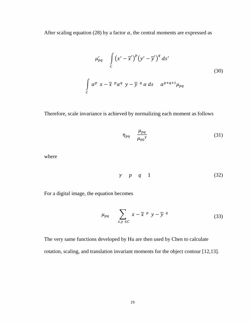
After scaling equation (28) by a factor 𝛼𝛼, the central moments are expressed as
𝜇𝜇𝑝𝑝𝑝𝑝′ = ��𝑥𝑥′ − 𝑥𝑥′�
𝑝𝑝�𝑦𝑦′ − 𝑦𝑦′�
𝑝𝑝 𝑑𝑑𝑠𝑠′
𝐶𝐶
=
� 𝛼𝛼𝑝𝑝(𝑥𝑥 − 𝑥𝑥)𝑝𝑝𝛼𝛼𝑝𝑝(𝑦𝑦 − 𝑦𝑦)𝑝𝑝 𝛼𝛼 𝑑𝑑𝑠𝑠𝐶𝐶
= 𝛼𝛼𝑝𝑝+𝑝𝑝+1𝜇𝜇𝑝𝑝𝑝𝑝
(30)
Therefore, scale invariance is achieved by normalizing each moment as follows
𝜂𝜂𝑝𝑝𝑝𝑝 =𝜇𝜇𝑝𝑝𝑝𝑝𝜇𝜇00𝛾𝛾
(31)
where
𝛾𝛾 = 𝑝𝑝 + 𝑞𝑞 + 1 (32)
For a digital image, the equation becomes
𝜇𝜇𝑝𝑝𝑝𝑝 = � (𝑥𝑥 − 𝑥𝑥)𝑝𝑝(𝑦𝑦 − 𝑦𝑦)𝑝𝑝(𝑥𝑥,𝑦𝑦)∈𝐶𝐶
(33)
The very same functions developed by Hu are then used by Chen to calculate
rotation, scaling, and translation invariant moments for the object contour [12,13].
20
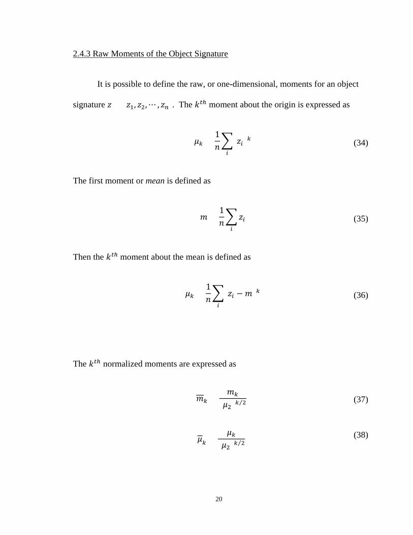
2.4.3 Raw Moments of the Object Signature
It is possible to define the raw, or one-dimensional, moments for an object
signature 𝑧𝑧 = [𝑧𝑧1, 𝑧𝑧2,⋯ , 𝑧𝑧𝑛𝑛]. The 𝑘𝑘𝑡𝑡ℎ moment about the origin is expressed as
𝜇𝜇𝑘𝑘 =1𝑚𝑚�(𝑧𝑧𝑖𝑖)𝑘𝑘𝑖𝑖
(34)
The first moment or mean is defined as
𝑚𝑚 =1𝑚𝑚�𝑧𝑧𝑖𝑖𝑖𝑖
(35)
Then the 𝑘𝑘𝑡𝑡ℎ moment about the mean is defined as
𝜇𝜇𝑘𝑘 =1𝑚𝑚�(𝑧𝑧𝑖𝑖 − 𝑚𝑚)𝑘𝑘𝑖𝑖
(36)
The 𝑘𝑘𝑡𝑡ℎ normalized moments are expressed as
𝑚𝑚𝑘𝑘 =𝑚𝑚𝑘𝑘
(𝜇𝜇2)𝑘𝑘 2⁄ (37)
𝜇𝜇𝑘𝑘 =𝜇𝜇𝑘𝑘
(𝜇𝜇2)𝑘𝑘 2⁄ (38)
21
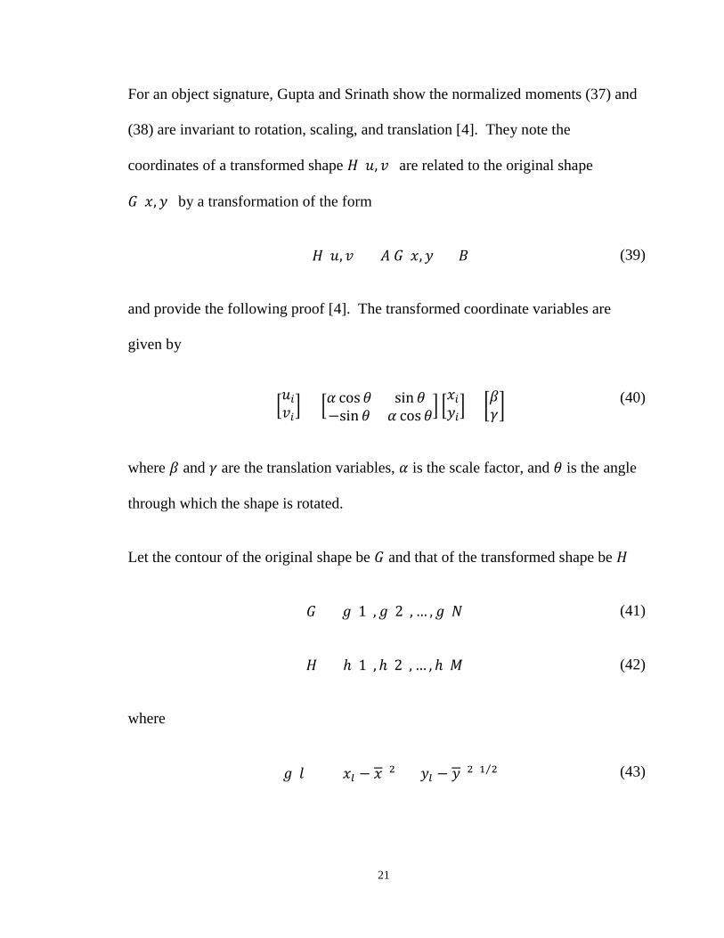
For an object signature, Gupta and Srinath show the normalized moments (37) and
(38) are invariant to rotation, scaling, and translation [4]. They note the
coordinates of a transformed shape 𝐻𝐻(𝑢𝑢, 𝑣𝑣) are related to the original shape
𝐺𝐺(𝑥𝑥,𝑦𝑦) by a transformation of the form
𝐻𝐻(𝑢𝑢, 𝑣𝑣) = 𝐴𝐴 𝐺𝐺(𝑥𝑥,𝑦𝑦) + 𝐵𝐵 (39)
and provide the following proof [4]. The transformed coordinate variables are
given by
�𝑢𝑢𝑖𝑖𝑣𝑣𝑖𝑖� = �𝛼𝛼 cos 𝜃𝜃 sin 𝜃𝜃
−sin 𝜃𝜃 𝛼𝛼 cos 𝜃𝜃� �𝑥𝑥𝑖𝑖𝑦𝑦𝑖𝑖� + �𝛽𝛽𝛾𝛾�
(40)
where 𝛽𝛽 and 𝛾𝛾 are the translation variables, 𝛼𝛼 is the scale factor, and 𝜃𝜃 is the angle
through which the shape is rotated.
Let the contour of the original shape be 𝐺𝐺 and that of the transformed shape be 𝐻𝐻
𝐺𝐺 = [𝑔𝑔(1),𝑔𝑔(2), … ,𝑔𝑔(𝑁𝑁)] (41)
𝐻𝐻 = [ℎ(1),ℎ(2), … ,ℎ(𝑀𝑀)] (42)
where
𝑔𝑔(𝑙𝑙) = [(𝑥𝑥𝑙𝑙 − 𝑥𝑥)2 + (𝑦𝑦𝑙𝑙 − 𝑦𝑦)2]1 2⁄ (43)
22
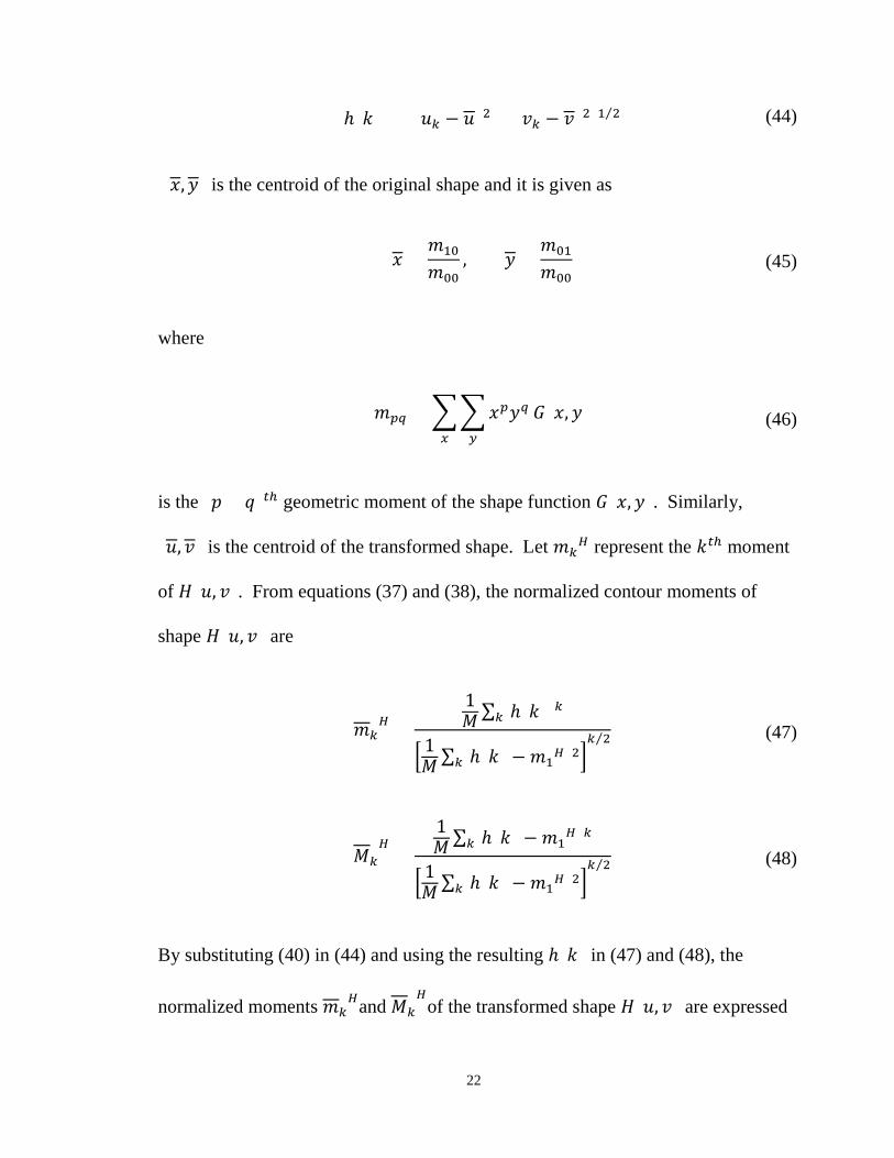
ℎ(𝑘𝑘) = [(𝑢𝑢𝑘𝑘 − 𝑢𝑢)2 + (𝑣𝑣𝑘𝑘 − 𝑣𝑣)2]1 2⁄ (44)
(𝑥𝑥,𝑦𝑦) is the centroid of the original shape and it is given as
𝑥𝑥 =𝑚𝑚10
𝑚𝑚00, 𝑦𝑦 =
𝑚𝑚01
𝑚𝑚00 (45)
where
𝑚𝑚𝑝𝑝𝑝𝑝 = ��𝑥𝑥𝑝𝑝𝑦𝑦𝑝𝑝𝑦𝑦
𝐺𝐺(𝑥𝑥,𝑦𝑦)𝑥𝑥
(46)
is the (𝑝𝑝 + 𝑞𝑞)𝑡𝑡ℎ geometric moment of the shape function 𝐺𝐺(𝑥𝑥,𝑦𝑦). Similarly,
(𝑢𝑢, 𝑣𝑣) is the centroid of the transformed shape. Let 𝑚𝑚𝑘𝑘𝐻𝐻 represent the 𝑘𝑘𝑡𝑡ℎ moment
of 𝐻𝐻(𝑢𝑢, 𝑣𝑣). From equations (37) and (38), the normalized contour moments of
shape 𝐻𝐻(𝑢𝑢, 𝑣𝑣) are
𝑚𝑚𝑘𝑘𝐻𝐻 =
1𝑀𝑀∑ [ℎ(𝑘𝑘)]𝑘𝑘𝑘𝑘
�1𝑀𝑀∑ [ℎ(𝑘𝑘) −𝑚𝑚1
𝐻𝐻]2𝑘𝑘 �𝑘𝑘 2⁄ (47)
𝑀𝑀𝑘𝑘𝐻𝐻
=1𝑀𝑀∑ [ℎ(𝑘𝑘) −𝑚𝑚1
𝐻𝐻]𝑘𝑘𝑘𝑘
�1𝑀𝑀∑ [ℎ(𝑘𝑘) −𝑚𝑚1
𝐻𝐻]2𝑘𝑘 �𝑘𝑘 2⁄ (48)
By substituting (40) in (44) and using the resulting ℎ(𝑘𝑘) in (47) and (48), the
normalized moments 𝑚𝑚𝑘𝑘𝐻𝐻and 𝑀𝑀𝑘𝑘
𝐻𝐻of the transformed shape 𝐻𝐻(𝑢𝑢, 𝑣𝑣) are expressed
23
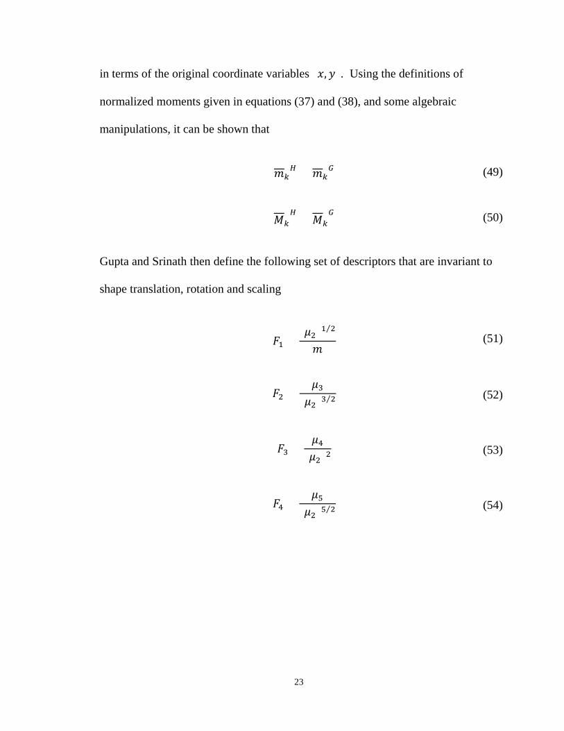
in terms of the original coordinate variables (𝑥𝑥,𝑦𝑦). Using the definitions of
normalized moments given in equations (37) and (38), and some algebraic
manipulations, it can be shown that
𝑚𝑚𝑘𝑘𝐻𝐻 = 𝑚𝑚𝑘𝑘
𝐺𝐺 (49)
𝑀𝑀𝑘𝑘𝐻𝐻
= 𝑀𝑀𝑘𝑘𝐺𝐺
(50)
Gupta and Srinath then define the following set of descriptors that are invariant to
shape translation, rotation and scaling
𝐹𝐹1 =
(𝜇𝜇2)1 2⁄
𝑚𝑚 (51)
𝐹𝐹2 =𝜇𝜇3
(𝜇𝜇2)3 2⁄ (52)
𝐹𝐹3 =𝜇𝜇4
(𝜇𝜇2)2 (53)
𝐹𝐹4 =𝜇𝜇5
(𝜇𝜇2)5 2⁄ (54)
24
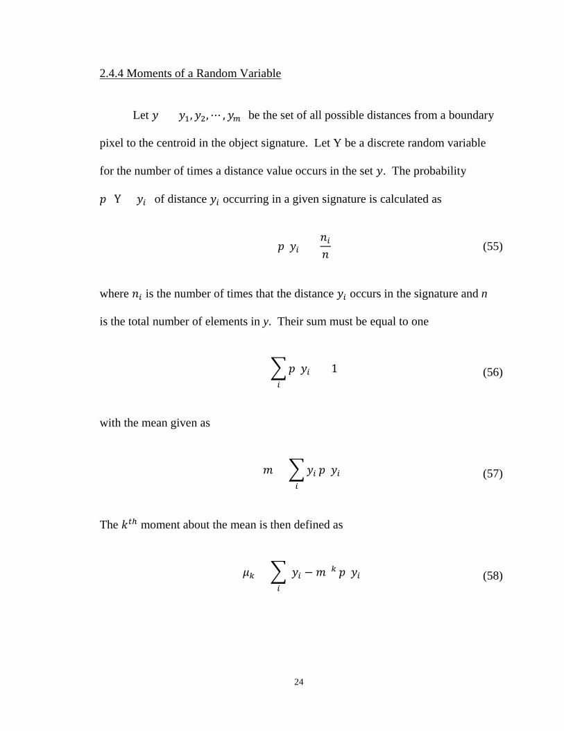
2.4.4 Moments of a Random Variable
Let 𝑦𝑦 = [𝑦𝑦1,𝑦𝑦2,⋯ , 𝑦𝑦𝑚𝑚] be the set of all possible distances from a boundary
pixel to the centroid in the object signature. Let Y be a discrete random variable
for the number of times a distance value occurs in the set 𝑦𝑦. The probability
𝑝𝑝( Y = 𝑦𝑦𝑖𝑖) of distance 𝑦𝑦𝑖𝑖 occurring in a given signature is calculated as
𝑝𝑝(𝑦𝑦𝑖𝑖) =𝑚𝑚𝑖𝑖𝑚𝑚
(55)
where 𝑚𝑚𝑖𝑖 is the number of times that the distance 𝑦𝑦𝑖𝑖 occurs in the signature and n
is the total number of elements in y. Their sum must be equal to one
�𝑝𝑝(𝑦𝑦𝑖𝑖)𝑖𝑖
= 1 (56)
with the mean given as
𝑚𝑚 = �𝑦𝑦𝑖𝑖𝑖𝑖
𝑝𝑝(𝑦𝑦𝑖𝑖) (57)
The 𝑘𝑘𝑡𝑡ℎ moment about the mean is then defined as
𝜇𝜇𝑘𝑘 = �(𝑦𝑦𝑖𝑖 − 𝑚𝑚)𝑘𝑘𝑖𝑖
𝑝𝑝(𝑦𝑦𝑖𝑖) (58)
25
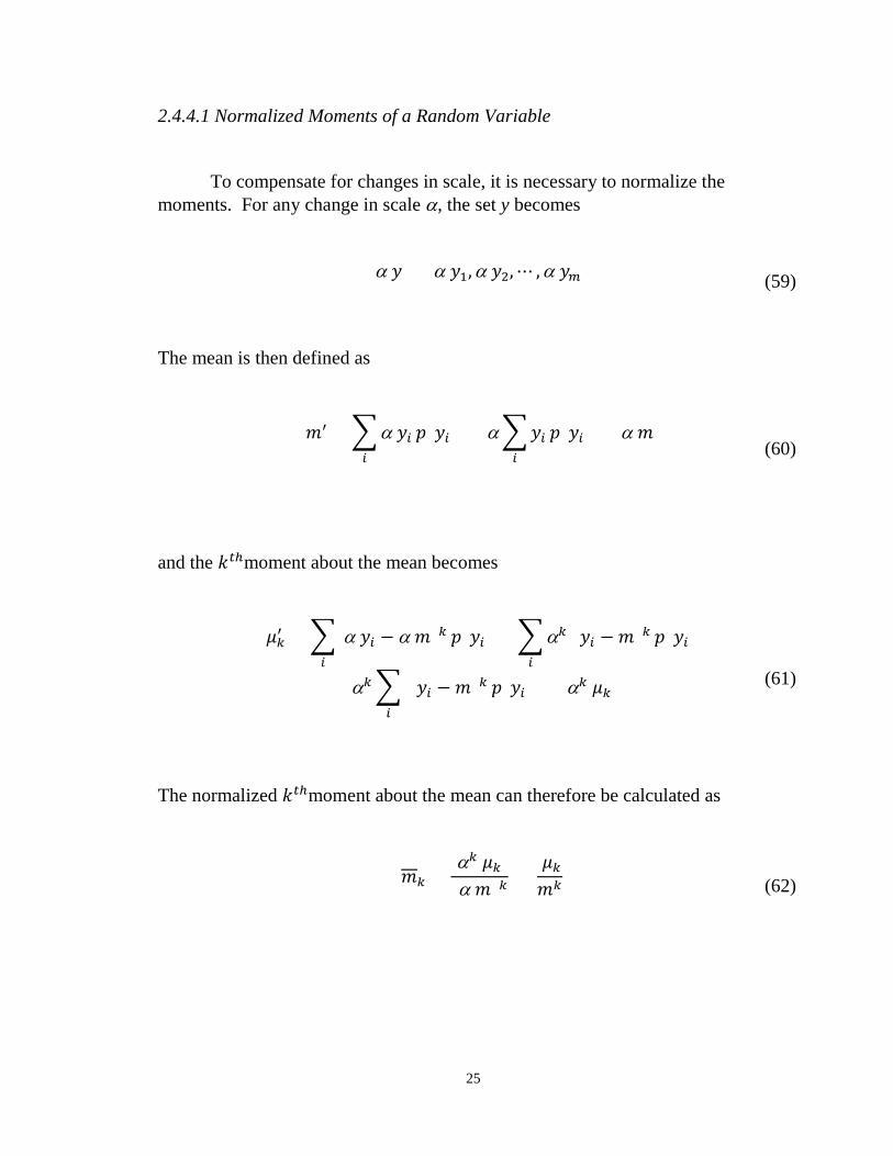
2.4.4.1 Normalized Moments of a Random Variable
To compensate for changes in scale, it is necessary to normalize the
moments. For any change in scale α, the set y becomes α 𝑦𝑦 = [α 𝑦𝑦1,α 𝑦𝑦2,⋯ ,α 𝑦𝑦𝑚𝑚]
(59)
The mean is then defined as 𝑚𝑚′ = �α 𝑦𝑦𝑖𝑖
𝑖𝑖
𝑝𝑝(𝑦𝑦𝑖𝑖) = α�𝑦𝑦𝑖𝑖𝑖𝑖
𝑝𝑝(𝑦𝑦𝑖𝑖) = α 𝑚𝑚
(60)
and the 𝑘𝑘𝑡𝑡ℎmoment about the mean becomes 𝜇𝜇𝑘𝑘′ = �(α 𝑦𝑦𝑖𝑖 − α 𝑚𝑚)𝑘𝑘
𝑖𝑖
𝑝𝑝(𝑦𝑦𝑖𝑖) = �α𝑘𝑘 (𝑦𝑦𝑖𝑖 − 𝑚𝑚)𝑘𝑘𝑖𝑖
𝑝𝑝(𝑦𝑦𝑖𝑖)
= α𝑘𝑘� (𝑦𝑦𝑖𝑖 − 𝑚𝑚)𝑘𝑘𝑖𝑖
𝑝𝑝(𝑦𝑦𝑖𝑖) = α𝑘𝑘 𝜇𝜇𝑘𝑘
(61)
The normalized 𝑘𝑘𝑡𝑡ℎmoment about the mean can therefore be calculated as
𝑚𝑚𝑘𝑘 =α𝑘𝑘 𝜇𝜇𝑘𝑘
(α 𝑚𝑚)𝑘𝑘=
𝜇𝜇𝑘𝑘𝑚𝑚𝑘𝑘
(62)
26
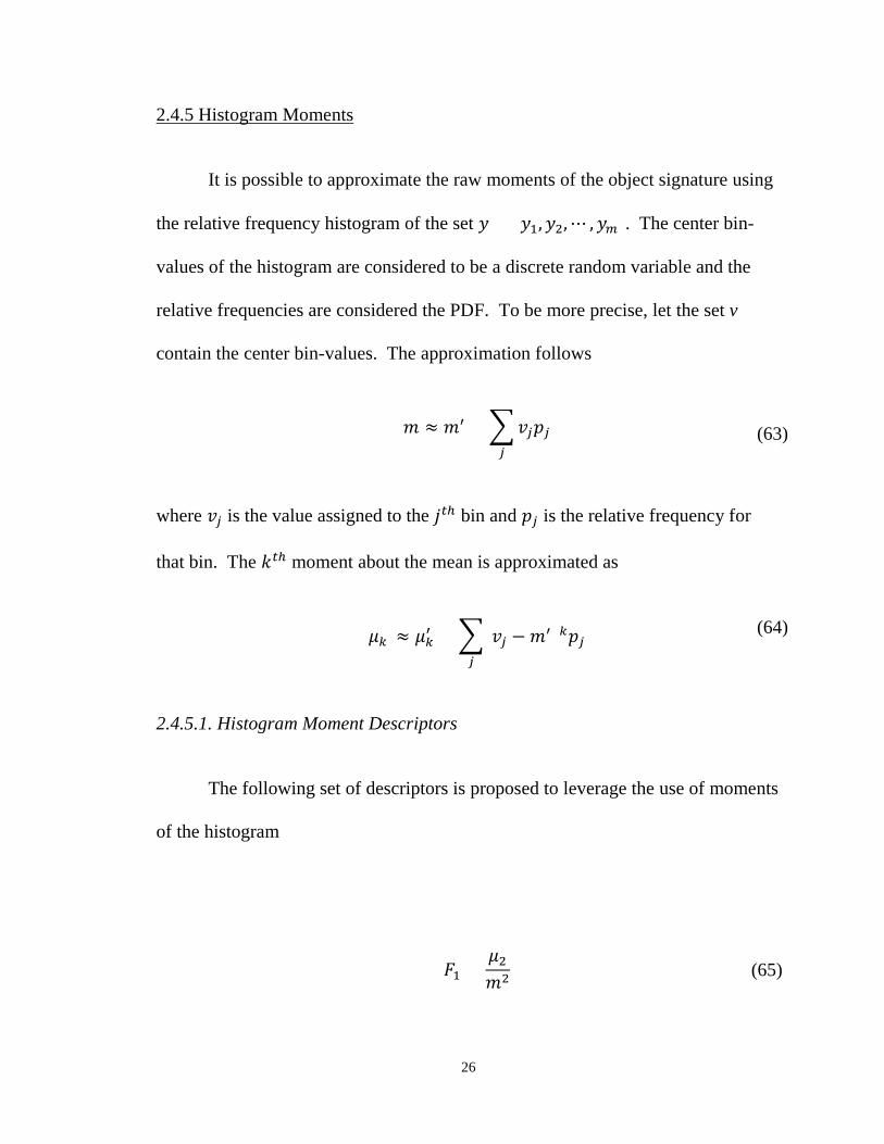
2.4.5 Histogram Moments
It is possible to approximate the raw moments of the object signature using
the relative frequency histogram of the set 𝑦𝑦 = [𝑦𝑦1,𝑦𝑦2,⋯ ,𝑦𝑦𝑚𝑚]. The center bin-
values of the histogram are considered to be a discrete random variable and the
relative frequencies are considered the PDF. To be more precise, let the set v
contain the center bin-values. The approximation follows
𝑚𝑚 ≈ 𝑚𝑚′ = �𝑣𝑣𝑗𝑗𝑝𝑝𝑗𝑗𝑗𝑗
(63)
where 𝑣𝑣𝑗𝑗 is the value assigned to the 𝑗𝑗𝑡𝑡ℎ bin and 𝑝𝑝𝑗𝑗 is the relative frequency for
that bin. The 𝑘𝑘𝑡𝑡ℎ moment about the mean is approximated as
𝜇𝜇𝑘𝑘 ≈ 𝜇𝜇𝑘𝑘′ = �(𝑣𝑣𝑗𝑗 − 𝑚𝑚′)𝑘𝑘𝑝𝑝𝑗𝑗𝑗𝑗
(64)
2.4.5.1. Histogram Moment Descriptors
The following set of descriptors is proposed to leverage the use of moments
of the histogram
𝐹𝐹1 =𝜇𝜇2𝑚𝑚2 (65)
27
𝐹𝐹2 =𝜇𝜇3𝑚𝑚3 (66)
𝐹𝐹3 =𝜇𝜇4𝑚𝑚4 (67)
The second, third, and fourth moments of the histogram of the object signature are
each divided by the first moment raised to the second, third, and fourth power
respectively. This ensures the descriptors are invariant to scaling. Since the
object signature is never zero in our experiments, the mean is always non-zero and
hence division by zero is not a concern. These descriptors only require the use of
four moments of the histogram compared to the five raw moments used by Gupta
and Srinath’s set of four descriptors.
2.5 Fourier Descriptors
The Fourier Descriptor is a technique used for representing shapes. They
are simple to compute, intuitive, and easy to normalize. In addition, they are
robust to noise and capture both global and local features [5]. The descriptors
represent the shape of the object in a frequency domain and avoid the high cost of
matching shape signatures in the spatial domain [6]. The Discrete Fourier
28
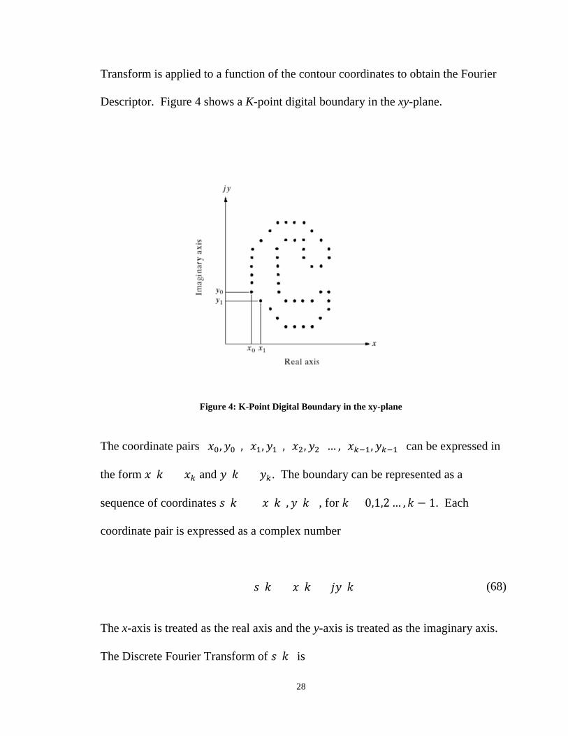
Transform is applied to a function of the contour coordinates to obtain the Fourier
Descriptor. Figure 4 shows a K-point digital boundary in the xy-plane.
Figure 4: K-Point Digital Boundary in the xy-plane
The coordinate pairs (𝑥𝑥0,𝑦𝑦0), (𝑥𝑥1,𝑦𝑦1), (𝑥𝑥2,𝑦𝑦2) … , (𝑥𝑥𝑘𝑘−1,𝑦𝑦𝑘𝑘−1) can be expressed in
the form 𝑥𝑥(𝑘𝑘) = 𝑥𝑥𝑘𝑘 and 𝑦𝑦(𝑘𝑘) = 𝑦𝑦𝑘𝑘. The boundary can be represented as a
sequence of coordinates 𝑠𝑠(𝑘𝑘) = [𝑥𝑥(𝑘𝑘),𝑦𝑦(𝑘𝑘)], for 𝑘𝑘 = 0,1,2 … ,𝑘𝑘 − 1. Each
coordinate pair is expressed as a complex number
𝑠𝑠(𝑘𝑘) = 𝑥𝑥(𝑘𝑘) + 𝑗𝑗𝑦𝑦(𝑘𝑘) (68)
The x-axis is treated as the real axis and the y-axis is treated as the imaginary axis.
The Discrete Fourier Transform of 𝑠𝑠(𝑘𝑘) is
29
𝑎𝑎𝑛𝑛 = �𝑠𝑠(𝑘𝑘)𝑧𝑧−𝑗𝑗2𝜋𝜋𝑘𝑘 𝐾𝐾⁄
𝑘𝑘
(69)
for 𝑚𝑚 = 0,1, 2 … ,𝐾𝐾 − 1 [1]. The coefficients 𝑎𝑎𝑛𝑛 are referred to as the Fourier
Descriptors. The one-dimensional Discrete Fourier Transform of an object
signature can be calculated as
𝑎𝑎𝑛𝑛 =1𝑁𝑁�𝑧𝑧(𝑡𝑡)𝑧𝑧−𝑗𝑗2𝜋𝜋𝑛𝑛𝜋𝜋 𝑁𝑁⁄
𝑡𝑡
(70)
Where z(t) is the object signature for 𝑚𝑚 = 0,1, 2 … ,𝑁𝑁 − 1. Hu and Li explain that
rotation invariance of the Fourier Descriptors is achieved by ignoring the phase
information, only taking into consideration the magnitude values [6]. Scale
invariance for real-valued signatures is established by dividing the magnitude of
the first half descriptors by the DC components |𝑎𝑎0|. Since |𝑎𝑎0| is always the
largest coefficient, the values of the normalized descriptors should be in the range
from zero to one [6]
𝑉𝑉 = �𝑎𝑎1𝑎𝑎0� , �
𝑎𝑎2𝑎𝑎0� , �𝑎𝑎3𝑎𝑎0� , … , �
𝑎𝑎𝑁𝑁 2⁄
𝑎𝑎0� (71)
30
2.6 Mean Square Error
The Mean Square Error (MSE) is an average of the squared errors. In this
thesis we define error to be a distance between corresponding elements of two
descriptor feature vectors representing image objects. It is computed as follows
𝑀𝑀𝑀𝑀𝑀𝑀 =1𝑚𝑚��𝐹𝐹𝑘𝑘𝑖𝑖 − 𝐹𝐹𝑘𝑘𝑟𝑟�
2
𝑘𝑘
𝑘𝑘 = 1. .𝑚𝑚 (72)
where 𝐹𝐹𝑘𝑘𝑖𝑖 is the 𝑘𝑘𝑡𝑡ℎ element of the 𝑚𝑚 element vector representing object i and 𝐹𝐹𝑘𝑘𝑟𝑟 is
the 𝑘𝑘𝑡𝑡ℎ element of the 𝑚𝑚 element vector representing object r.
2.7 Confusion Matrix
Results of experiments are presented in this paper using a confusion matrix.
A confusion matrix is a matrix where element �𝑚𝑚𝑖𝑖,𝑗𝑗� of the matrix m is the Mean
Square Error (MSE) between the element assigned to row i and the element
assigned to column j. For each row in the matrix, the column with the lowest
MSE is considered a match. An MSE of zero is an exact match while a higher
MSE is indicative of dissimilarity between the two elements. An error occurs
when �𝑚𝑚𝑖𝑖,𝑗𝑗� is a match but the element assigned to row i is not the same as the
element assigned to row j.

31
2.8 Star-Convex
A set of points is considered convex if for any two points in the set, all
points on the line segment connecting the two points are included in the set. A set
is considered to be star-convex if there exists at least one point such that for any
other point in the set, all points on the line segment connecting the two points are
included in the set.
32
III. RELATED WORK
In this section, relevant research is discussed and compared to the method
presented in this paper. This thesis presents a novel method for recognizing
objects in images. The method utilizes a minimum number of moments of the
histogram of the object signature, and requires far less computation operations,
resulting in effective, accurate descriptors. Previous research has applied
moments to the entire image or directly to the contour or the object signature. This
is the first work that investigates applying moments to the histogram of the object
signature.
Hu presented the first significant research into the use of moments for two-
dimensional image analysis and recognition [7]. Based on the method of algebraic
invariants, Hu derived a set of seven moments using nonlinear combinations of
lower order regular moments. This set of moments is invariant to translation,
scaling, and rotation but is a region-based method that treats shapes as a whole.
The moments must be computed over all pixels of an object, including the
contour. This is in stark contrast to the method introduced in this work, which
utilizes moments of the histogram of the object signature. When calculating the
moments of the histogram of the object signature, only the center bin-values of the
constructed histogram are used. As a result, the savings in computation are
33
significant and provide computational complexity that is orders of magnitude
smaller than using every pixel of the image. In addition, the descriptors introduced
in this thesis only require computing four moments as opposed to seven, and only
pixels in the object contour are required.
Chen proposed a modified version of Hu’s method involving the same
moment invariants, requiring computation over just the pixels that make up the
object contour [12]. However, like Hu, Chen’s method requires computing seven
moments as opposed to the method introduced in this thesis which only requires
four. Although Chen’s method is computationally less costly than Hu’s, it uses
every pixel in the contour and therefore, in general, it is expected to be less
efficient than using the histogram of the object signature.
Mandal et al. offer an approach that employs statistical moments of a
random variable [15]. They suggest treating the intensity values of image pixels
as a random variable and using the normalized image histogram as an
approximation of the PDF for pixel intensities. Moments of the random variable
are then calculated and used to describe the object. This is a region-based
approach that requires consideration of all pixels in the object, including the
contour. Our method utilizing moments of the histogram of the object signature
only involve pixels that make up the contour of the object and since only the
34
center bin-values of the histogram are used to calculate moments, the savings in
computation are substantial.
Gonzales and Woods suggest representing a segment of the boundary for an
object as a one-dimensional function of an arbitrary variable [1]. The amplitude of
the function is treated as a discrete random variable and a normalized frequency
histogram is used to estimate the PDF for the random variable. Moments of the
random variable are then calculated and used to describe the shape. However, the
authors do not use the entire contour of the object nor do they use the object
signature.
Gupta and Srinath use the moments of a signature derived from the contour
pixels of an object to generate descriptors that are invariant to translation, rotation,
and scaling [4]. The paper, however, requires the contour pixels to be organized
into an ordered sequence before computing the Euclidean distance between
contour pixels and the object centroid to produce the signature. In addition, the
authors do not group the signature values into a histogram before calculating the
moments. Consequently, they use every element of the object signature to
calculate each moment in contrast to the method introduced in this paper, which
only uses the center value of each bin in the histogram. In general, far less
computation is necessary. Furthermore, Gupta and Srinath require five moments
to derive their descriptors. The method introduced in this work only requires four.
35
IV. EXPERIMENTAL SETUP
This section discusses the setup of the experiments and how results are
presented and evaluated. The goal of the experiments is to compare the
effectiveness of various descriptors in recognizing objects that have been
translated, scaled, and rotated. The descriptors evaluated in these experiments are
as follows:
1. Moment Invariants 2. Moment Invariants of the Object Contour 3. 2D Fourier Descriptors of the Object Contour 4. Moments of the Object Signature 5. Moments of the Histogram of the Object Signature 6. 1D Fourier Descriptors of the Object Signature
4.1 Software The experiments for this thesis were developed and implemented using the
MATLAB computing environment (version 7.14.0.739).
4.2 Hardware
A 2.8 GHz Intel Core i5 processor running 64-bit Mac OS X version 10.9.5
was used to run the experiments.
36
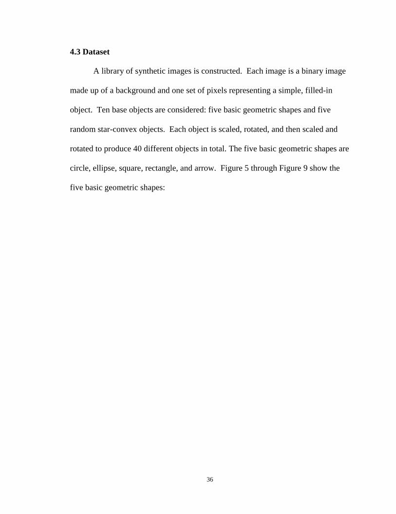
4.3 Dataset
A library of synthetic images is constructed. Each image is a binary image
made up of a background and one set of pixels representing a simple, filled-in
object. Ten base objects are considered: five basic geometric shapes and five
random star-convex objects. Each object is scaled, rotated, and then scaled and
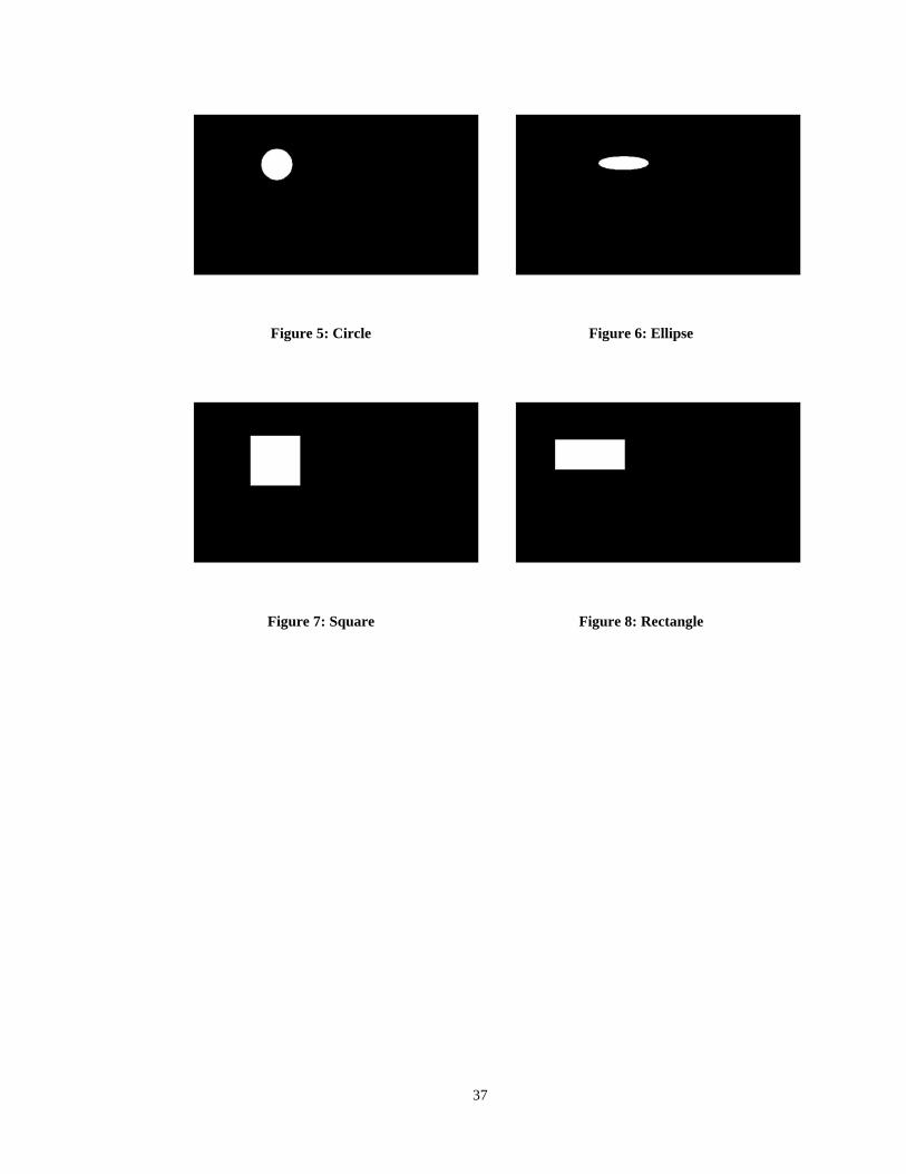
rotated to produce 40 different objects in total. The five basic geometric shapes are
circle, ellipse, square, rectangle, and arrow. Figure 5 through Figure 9 show the
five basic geometric shapes:
37
Figure 5: Circle
Figure 6: Ellipse
Figure 7: Square
Figure 8: Rectangle
38
Figure 9: Arrow
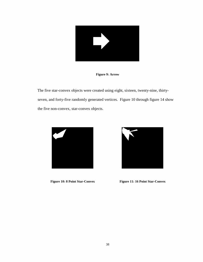
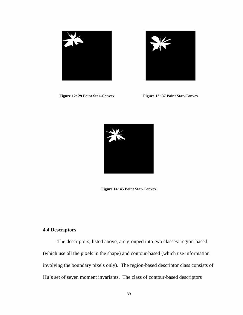
The five star-convex objects were created using eight, sixteen, twenty-nine, thirty-
seven, and forty-five randomly generated vertices. Figure 10 through figure 14 show
the five non-convex, star-convex objects.
Figure 10: 8 Point Star-Convex
Figure 11: 16 Point Star-Convex
39
Figure 12: 29 Point Star-Convex
Figure 13: 37 Point Star-Convex
Figure 14: 45 Point Star-Convex
4.4 Descriptors
The descriptors, listed above, are grouped into two classes: region-based
(which use all the pixels in the shape) and contour-based (which use information
involving the boundary pixels only). The region-based descriptor class consists of
Hu’s set of seven moment invariants. The class of contour-based descriptors
40
includes moments of the object signature, moments of the histogram of the object
signature, two-dimensional Fourier descriptors of the object contour, one-
dimensional Fourier descriptors of the object signature, and Chen’s application of
Hu’s moment invariants to the object contour. The object signature is obtained by
calculating the Euclidean distance from the centroid of the object to each pixel in
the object contour.
4.5 Process
In each experiment, a different descriptor is used to compare the objects in
the library against the objects in a database made up of the ten base objects. First,
the descriptor feature vectors are computed for all objects in the library and
database. Then a confusion matrix is constructed where each row is assigned the
feature vector representing an input object 𝑂𝑂𝑙𝑙 from the library and each column is
assigned a feature vector representing a reference object 𝑂𝑂𝑑𝑑 from the database.
The result is a 40 x 10 matrix. Each element �𝑚𝑚𝑖𝑖,𝑟𝑟� of the matrix is the Mean
Square Error (MSE) between the feature vector assigned to row i and the feature
vector assigned to column r. For each row, the column with the smallest MSE is
considered a match. An MSE of zero is an exact match while a higher MSE is
indicative of dissimilarity. If the feature vectors representing two objects are a
match, then the objects they represent are considered to be a match. An error
occurs when an input object 𝑂𝑂𝑙𝑙 from the library is a match with a reference object
𝑂𝑂𝑑𝑑 from the database but the two objects are not the same. For example, if the
41
scaled and rotated arrow object from the library is identified as a match with the
square object from the database, the result is considered an error.
4.6 Comparison
Descriptors are compared using recognition accuracy in addition to the
quality of recognition in the experiment. An effective descriptor should have an
MSE close to zero for matches and a relatively large MSE for non-matches. For
these experiments, the Quality Recognition score is computed by taking the ratio
of average MSE for matches, 𝑀𝑀𝑚𝑚, to average MSE for non-matches, 𝑀𝑀𝑛𝑛
𝑞𝑞 =𝑀𝑀𝑚𝑚
𝑀𝑀𝑛𝑛
The quality of recognition improves as the 𝑞𝑞 number approaches zero.
The Recognition Rate is the ratio of correct matches to total possible
correct matches
𝑧𝑧 =𝑀𝑀 − 𝑀𝑀𝑀𝑀

42
where, E is the total number of errors and M is the total number of possible correct
matches. For each of the experiments in this thesis, 𝑀𝑀 = 40.
43
V. EXPERIMENTS AND RESULTS
In this section, the experiments conducted as part of this thesis are
discussed. Six experiments in total are performed. For each experiment, a
confusion matrix that displays the recognition accuracy is presented. The results
of each experiment are compared using recognition accuracy. Quality of
recognition is used to contrast only those methods that achieve a 100% recognition
rate. In the resulting confusion matrices, matches are highlighted in yellow for
each experiment. An experiment with 100% recognition shows all matches along
the diagonal. Matches that are off the diagonal are incorrect and count against the
recognition rate.
Experiment 1
The first experiment evaluates Hu’s set of seven moment-invariant
descriptors as shown in equations (20) – (26). Table 1 shows the confusion matrix
derived in the experiment.
44
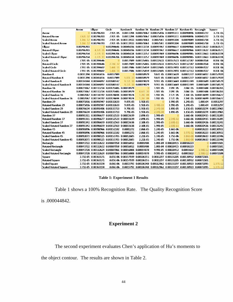
Table 1: Experiment 1 Results
Table 1 shows a 100% Recognition Rate. The Quality Recognition Score
is .000044842.
Experiment 2
The second experiment evaluates Chen’s application of Hu’s moments to
the object contour. The results are shown in Table 2.
45
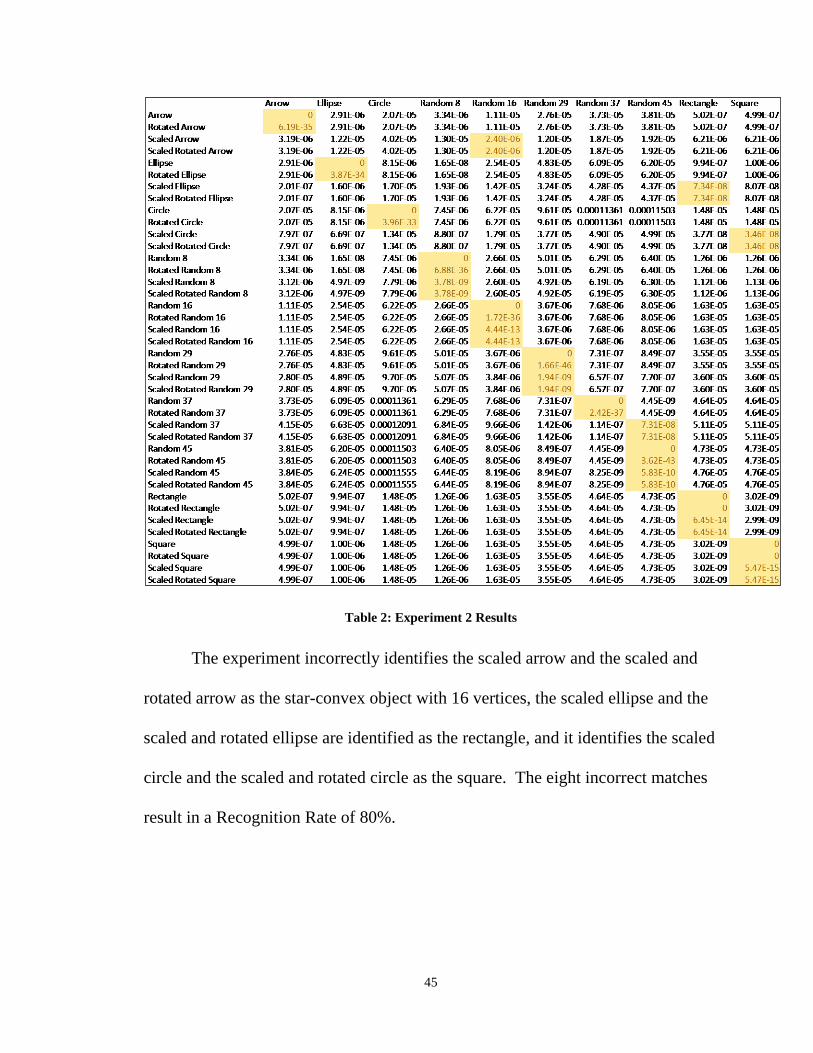
Table 2: Experiment 2 Results
The experiment incorrectly identifies the scaled arrow and the scaled and
rotated arrow as the star-convex object with 16 vertices, the scaled ellipse and the
scaled and rotated ellipse are identified as the rectangle, and it identifies the scaled
circle and the scaled and rotated circle as the square. The eight incorrect matches
result in a Recognition Rate of 80%.
46
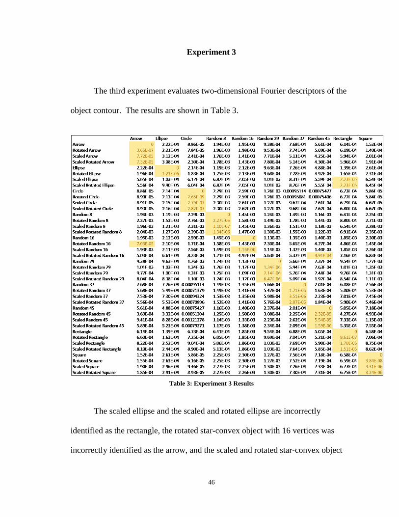
Experiment 3
The third experiment evaluates two-dimensional Fourier descriptors of the
object contour. The results are shown in Table 3.
Table 3: Experiment 3 Results
The scaled ellipse and the scaled and rotated ellipse are incorrectly
identified as the rectangle, the rotated star-convex object with 16 vertices was
incorrectly identified as the arrow, and the scaled and rotated star-convex object
47
with 16 vertices is misidentified as the star-convex object with 45 vertices. The
resulting Recognition Rate is 90%.
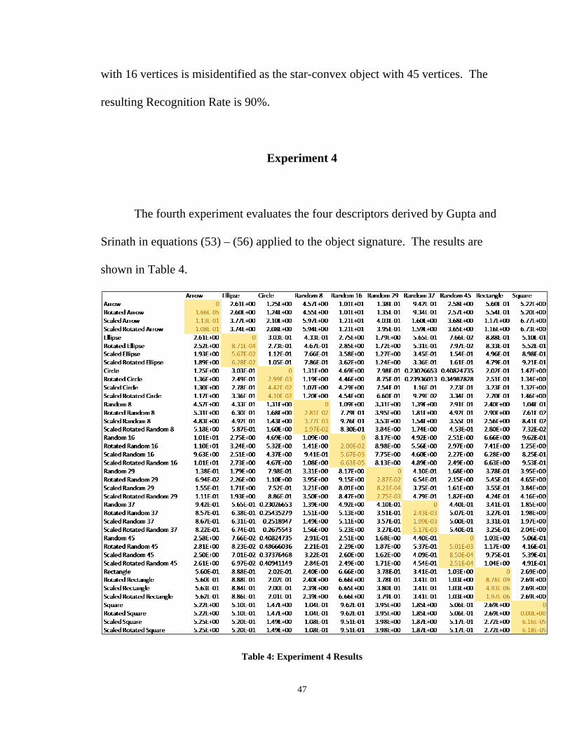
Experiment 4
The fourth experiment evaluates the four descriptors derived by Gupta and
Srinath in equations (53) – (56) applied to the object signature. The results are
shown in Table 4.
Table 4: Experiment 4 Results
48
The experiment correctly identifies all objects with zero errors, therefore
the resulting Recognition Rate is 100%. The Quality Recognition Score is
calculated to be 0.0673.
Experiment 5
The fifth experiment evaluates the application of moments to the histogram
of the object signature. For this experiment the new set of descriptors introduced
in equations (65) – (67) are used. The results are shown in Table 5.
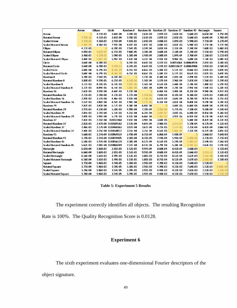
49
Table 5: Experiment 5 Results
The experiment correctly identifies all objects. The resulting Recognition
Rate is 100%. The Quality Recognition Score is 0.0128.
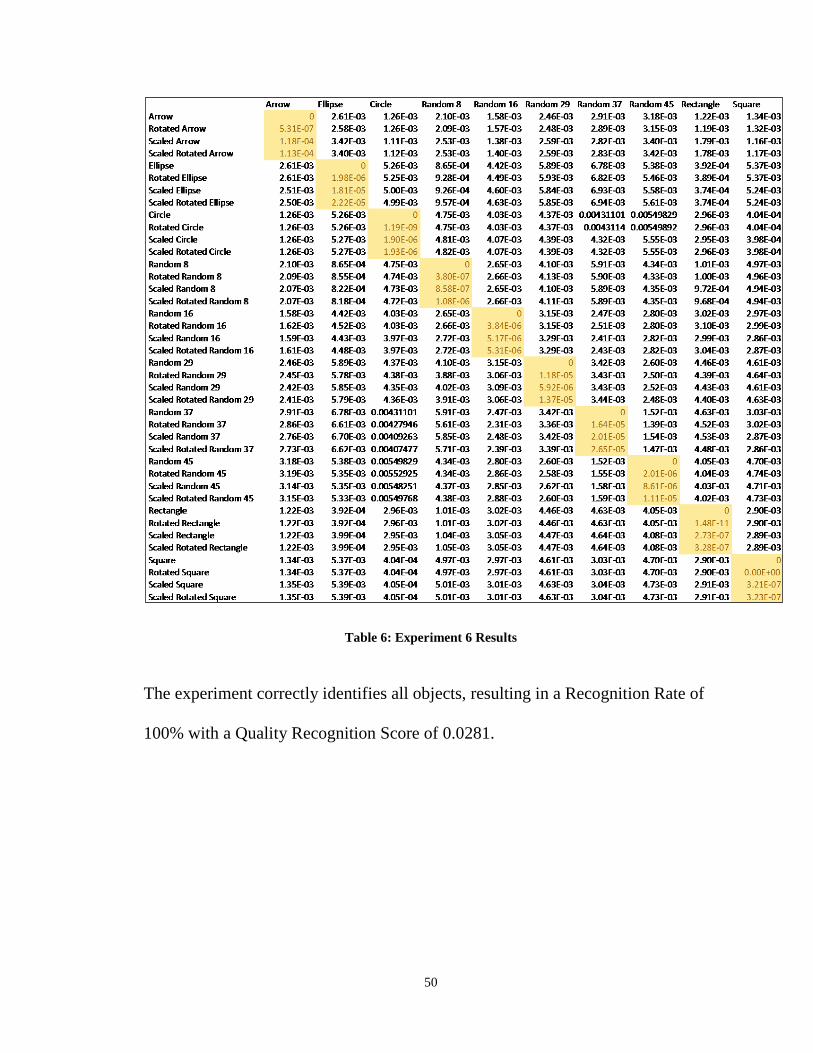
Experiment 6
The sixth experiment evaluates one-dimensional Fourier descriptors of the
object signature.
50
Table 6: Experiment 6 Results
The experiment correctly identifies all objects, resulting in a Recognition Rate of
100% with a Quality Recognition Score of 0.0281.
51
VI. RESULTS EVALUATION
This section evaluates the results of the experiments outlined in the
previous chapter. Six experiments in total are performed, each conducted to
evaluate the use of specific descriptors to recognize objects in a segmented image.
First, the Recognition Rate is compared. Next, the Quality of Recognition is used
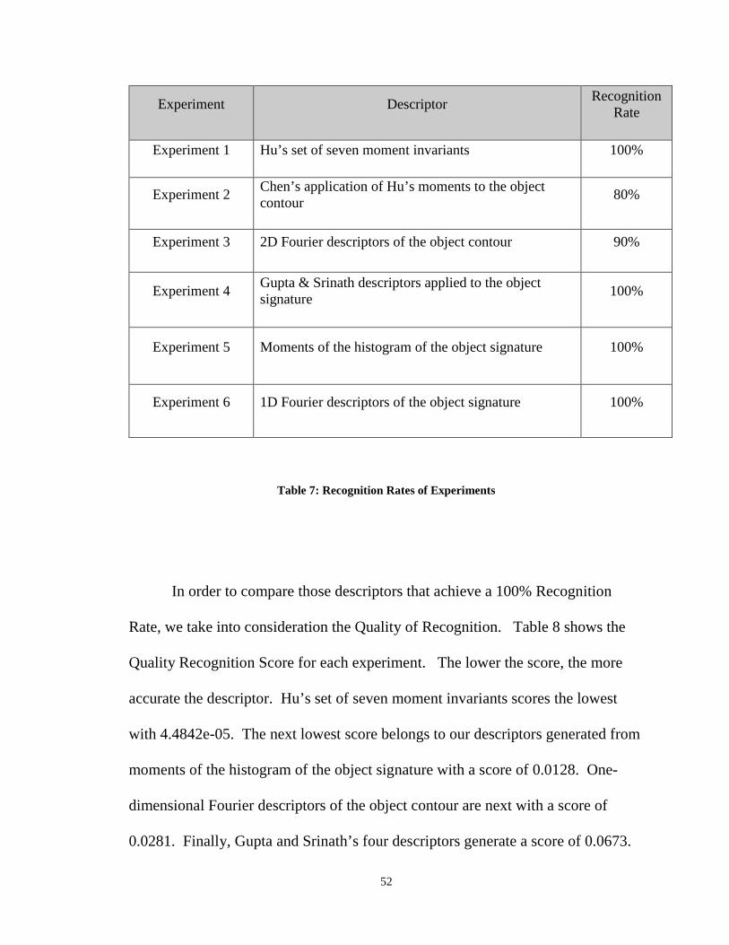
to differentiate between the methods that achieve a 100% Recognition Rate. Table
7 shows the Recognition Rate of each of the experiments. Four of the experiments
correctly identify every object in the library and achieve a 100% Recognition
Rate. Those experiments are Hu’s set of seven moment-invariant descriptors,
Gupta and Srinath’s set of four descriptors of the object signature, the set of three
descriptors introduced in this work generated from moments of the histogram of
the object signature, and one-dimensional Fourier descriptors of the object
signature. Chen’s application of Hu’s moments to the object contour incorrectly
identify eight objects and achieves an 80% Recognition Rate. Two-dimensional
Fourier descriptors of the object contour incorrectly identify four objects and
achieve a 90% recognition rate.
52
Experiment Descriptor Recognition Rate
Experiment 1 Hu’s set of seven moment invariants 100%
Experiment 2 Chen’s application of Hu’s moments to the object contour 80%
Experiment 3 2D Fourier descriptors of the object contour 90%
Experiment 4 Gupta & Srinath descriptors applied to the object signature 100%
Experiment 5 Moments of the histogram of the object signature 100%
Experiment 6 1D Fourier descriptors of the object signature 100%
Table 7: Recognition Rates of Experiments
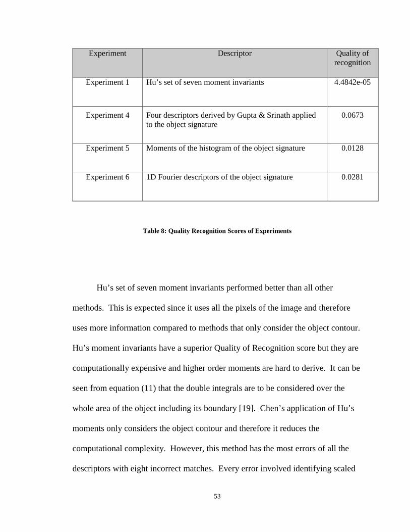
In order to compare those descriptors that achieve a 100% Recognition
Rate, we take into consideration the Quality of Recognition. Table 8 shows the
Quality Recognition Score for each experiment. The lower the score, the more
accurate the descriptor. Hu’s set of seven moment invariants scores the lowest
with 4.4842e-05. The next lowest score belongs to our descriptors generated from
moments of the histogram of the object signature with a score of 0.0128. One-
dimensional Fourier descriptors of the object contour are next with a score of
0.0281. Finally, Gupta and Srinath’s four descriptors generate a score of 0.0673.
53
Experiment Descriptor Quality of recognition
Experiment 1 Hu’s set of seven moment invariants 4.4842e-05
Experiment 4 Four descriptors derived by Gupta & Srinath applied to the object signature
0.0673
Experiment 5 Moments of the histogram of the object signature 0.0128
Experiment 6 1D Fourier descriptors of the object signature 0.0281
Table 8: Quality Recognition Scores of Experiments
Hu’s set of seven moment invariants performed better than all other
methods. This is expected since it uses all the pixels of the image and therefore
uses more information compared to methods that only consider the object contour.
Hu’s moment invariants have a superior Quality of Recognition score but they are
computationally expensive and higher order moments are hard to derive. It can be
seen from equation (11) that the double integrals are to be considered over the
whole area of the object including its boundary [19]. Chen’s application of Hu’s
moments only considers the object contour and therefore it reduces the
computational complexity. However, this method has the most errors of all the
descriptors with eight incorrect matches. Every error involved identifying scaled
54
objects. Using only the boundary pixels reduces the amount of information to be
processed. The method introduced in this work, taking moments of the histogram
of the object signature, only uses the center bin-values of the constructed
histogram to calculate moments. The computational costs are orders of magnitude
smaller than methods that use every pixel of the image or even just pixels of the
object contour.
The descriptors based on moments of the histogram of the object signature
introduced in this thesis show an improvement over those based on raw moments,
such as the methods proposed by Gupta and Srinath. Although both sets of
descriptors achieve a 100% Recognition Rate, the descriptors derived in this work
achieve a better Quality of Recognition score. The effect of binning the data when
constructing the histogram compensates for any noise introduced due to scaling an
object. In addition, only four moments are required compared to Gupta and
Srinath, who use five. The computational complexity is reduced by the method
introduced in this thesis, since the moments are calculated using the bin-values of
the histogram of the object signature. The calculations used in deriving Gupta and
Srinath’s descriptors involve every element of the object signature. The result is a
significant improvement in efficiency.
Based on the results of the experiments, the method introduced in this thesis,
taking the moments of the histogram of the object signature, proves to be more
accurate than all other methods with the exception of Hu’s moment invariants.
55
Although Hu’s moment invariants are more accurate, taking moments of the
histogram of the object signature is computationally less expensive.
Conclusion
With the explosion of data generated in the form of images and video, there
is a growing need to develop methods and techniques to automate their analysis,
such as recognizing and matching objects in images. The goal of this thesis is to
compare various descriptors that do just that. The six experiments show that the
region-based moment invariants developed by Hu performed best. However, it
was demonstrated that Fourier Descriptors and descriptors that utilize moments of
the object signature are viable alternatives. Among those, the set of descriptors
derived in this work based on moments of the histogram of the object signature,
have the best Quality of Recognition. In addition, because the method introduced
in this thesis uses the histogram when calculating moments, the computational
costs are orders of magnitude smaller than other descriptors discussed.
Future research into the computational complexity of these algorithms will
better quantify their efficiency. Experiments with natural images are a logical
next step for investigation as well. Additional translation, rotation, and scaling of
objects can be added to improve comparisons between descriptors.
56
BIBLIOGRAPHY
[1] R.C. Gonzalez and R.E. Woods, Digital Image Processing, 3rd ed. Upper Saddle River: Prentice-Hall, 2008. [2] R.A. Baggs and D.E. Tamir, “Non-rigid Image Registration”, Proceedings of the Florida Artificial Intelligence Research Symposium, Coconut Grove, FL, 2008. [3] D.E. Tamir, N. T. Shaked, W. J. Geerts, S. Dolev, “Compressive Sensing of Object-Signature”, Proceedings of the 3rd International Workshop on Optical Super Computing, Bertinoro, Italy, 2010. [4] L. Gupta and M.D. Srinath, “Contour sequence moments for the classification of closed planar shapes”, Pattern Recognition, vol. 20, no. 3, pp. 267-272, June, 1987. [5] P.L.E. Ekombo, N. Ennahnahi, M. Oumsis, M. Meknassi, “Application of affine invariant Fourier descriptor to shape-based image retrieval”, International Journal of Computer Science and Network Security, vol. 9, no. 7, pp. 240-247, July, 2009. [6] Y. Hu and Z. Li, “An Improved Shape Signature for Shape Representation and Image Retrieval”, Journal of Software, vol. 8, no. 11, pp. 2925-2929, Nov., 2013. [7] M.K. Hu, “Visual pattern recognition by moment invariants”, IRE Transactions on Information Theory, vol. 8, Feb., 1962. [8] E. Slud. (Spring 2009). “Scaled Relative Frequency Histograms” (lecture notes) [Online]. Available: http://www.math.umd.edu/~slud/s430/Handouts/Histogram.pdf. [9] J. Flusser, T. Suk, B. Zitová., Moments and Moment Invariants in Pattern Recognition, Chichester, UK: John Wiley & Sons Ltd., 2009. [10] M. Yang, K. Kpalma, R. Joseph, “A Survey of Shape Feature Extraction Techniques”, Pattern Recognition, pp. 43-90, Nov., 2008. [11] R.J. Prokop and A.P. Reeves “A survey of moment-based techniques for unoccluded object representation and recognition”, CVGIP: Graphics Models and Image Processing, vol. 54, no. 5, pp. 438-460, Sept. 1992. [12] C.C. Chen, “Improved moment invariants for shape discrimination”, Pattern Recognition, vol. 26, pp. 683-686, May, 1993. [13] L. Keyes and A. Winstanley, “Using moment invariants for classifying shapes on large-scale maps”, Computers, Environment and Urban Systems, vol. 25, pp. 119-130, Jan., 2001.

57
[14] J. Žunić, “Shape Descriptors for Image Analysis”, Zbornik Radova MI-SANU, Vol. 15, pp. 5-38, 2012. [15] M.K. Mandal, T. Aboulnasr, S. Panchanathan, “Image indexing using moments and wavelets”, IEEE Transactions on Consumer Electronics., vol. 42, no. 3, pp. 557-565, Aug. 1996. [16] J. Han and M. Kamber, Data Mining: Concepts and Techniques, 2nd ed. San Francisco: Morgan Kaufmann, 2006.