object detection from registered visual and …etd.lib.metu.edu.tr/upload/12609671/index.pdf ·...

OBJECT DETECTION FROM REGISTERED VISUAL AND INFRARED

SEQUENCES WITH THE HELP OF ACTIVE CONTOURS

A THESIS SUBMITTED TO

THE GRADUATE SCHOOL OF NATURAL AND APPLIED SCIENCES

OF

MIDDLE EAST TECHNICAL UNIVERSITY

BY

HÜSEYİN YÜRÜK

IN PARTIAL FULLFILLMENT OF THE REQUIREMENTS

FOR

THE DEGREE OF MASTER OF SCIENCE

IN

ELECTRICAL AND ELECTRONICS ENGINEERING

JULY 2008

Approval of the thesis:

OBJECT DETECTION FROM REGISTERED VISUAL AND INFRARED

SEQUENCES WITH THE HELP OF ACTIVE CONTOURS

submitted by HÜSEYİN YÜRÜK in partial fulfillment of the requirements for the

degree of Master of Science in Electrical and Electronics Engineering

Department, Middle East Technical University by,

Prof. Dr. Canan Özgen

Dean, Graduate School of Natural and Applied Sciences

Prof. Dr. İsmet Erkmen

Head of Department, Electrical and Electronics Engineering

Assist. Prof. Dr. İlkay Ulusoy

Supervisor, Electrical and Electronics Engineering Dept., METU

Examining Committee Members:

Prof. Dr. Uğur HALICI

Electrical and Electronics Engineering Dept., METU

Assist. Prof. Dr. İlkay Ulusoy


Prof. Dr. Gözde Bozdağı Akar


Assist. Prof. Dr. Alptekin Temizel

Informatics Institute, METU

MSc. İlker Gürel

ASELSAN Inc.

Date:

iii

I hereby declare that all information in this document has been obtained and

presented in accordance with academic rules and ethical conduct. I also

declare that, as required by these rules and conduct, I have fully cited and

referenced all material and results that are not original to this work.

Name, Last name : Hüseyin YÜRÜK

Signature :

iv

ABSTRACT

OBJECT DETECTION FROM REGISTERED VISUAL

AND INFRARED SEQUENCES WITH THE HELP OF

ACTIVE CONTOURS

Yürük, Hüseyin

M. S., Department of Electrical and Electronics Engineering

Supervisor : Assist. Prof. Dr. İlkay Ulusoy

July 2008, 82 pages

Robust object detection from registered infrared and visible image streams is

proposed for outdoor surveillance. In doing this, halo effect in infrared images is

used as a benefit to extract object boundary by fitting active contour models (snake)

to the foreground regions where these regions are detected by using the useful

information from both visual and infrared domains together.

Synchronization and registration are performed for each infrared and visible image

couple. Various background modeling methods such as Single Gaussian, Non-

Parametric and Mixture of Gaussian models are implemented. For Single Gaussian

and Mixture of Gaussian background modeling, infrared, color intensity and color

channels domains are modelled separately. First of all, background subtraction is

applied in the infrared domain in order to find the initial foreground regions and

these are used as a mask for the foreground detection in the visible domain. After

removing the shadows from the foreground regions in the visible domain, pixel-

wise OR operation is applied between the foreground regions of the infrared and

v

visible couple and the final foreground mask is formed. For Non-Parametric

background modeling, all domains are used altogether to extract foreground

regions. For all background modelling methods, the resulting mask is used to get

the final foreground regions in the infrared image. Finally, snake is applied to each

connected component of the foreground regions on the infrared image for the

purpose of object detection.

Two datasets are used to demonstrate our results for human detection where

comparisons against manually segmented human regions and against other results in

the literature are presented.

Keywords : Background modeling, shadow detection, fusion of infrared and color

domain, application of snake algorithm

vi

ÖZ

AKTİF KONTURLAR YARDIMIYLA, BIRBIRIYLE

UYUMLANMIŞ RENKLİ VE KIZIL ÖTESİ

DİZİLERİNDEN NESNELERIN BULUNMASI

Yürük, Hüseyin

Yüksek Lisans, Elektrik Elektronik Mühendisliği Bölümü

Tez Yöneticisi :Dr. İlkay Ulusoy

Temmuz 2008, 82 sayfa

Bu tez kapsamında, dış alan güvenliği için birbiriyle uyumlanmış kızıl ötesi ve

renkli görüntü dizilerinden sağlam nesne bulunması önerilmiştir. Bu işi

gerçekleştirmek için, kızıl ötesinde bulunan “halo” etkisi, bir avantaj olarak,

nesnelerin sınırlarının, aktif kontur modellerin ön plan alanlarına uyarlanarak

çıkartılmasında kullanılmıştır. Ön plan, kızıl ötesi ve renkli alanlardan elde edilen

kullanışlı bilgilerin kullanılmasıyla bulunmaktadır.

Her bir kızıl ötesi ve renkli resim çifti için eşleme ve uyumlama işlemi

gerçekleştirilmektedir. Tekli Gaussian, parametrik olmayan ve karma Gaussian

modelleri gibi, bir çok arka plan modelleme metotları uygulanmıştır. Tekli ve

karışım Gaussian arka plan modelleri için, arka plan istatistiksel olarak her bir kızıl

ötesi, renk yoğunluğu ve kanalları alanında ayrı ayrı modellenmiştir. Arka plan

çıkarma işlemi ilk olarak kızıl ötesi alanda, ön planın çıkarılması için yapılmış ve

bu bölge renkli alanlarda arka plan çıkarma işleminde maske olarak kullanılmıştır.

Renkli alanın ön planında bulunan gölgeler çıkarıldıktan sonra, son maske, kızıl

vii

ötesi ve renkli çiftin ön plan bölgelerine, piksel bazında “veya” işlemi uygulanması

ile oluşturulur. Parametrik olmayan model için, bütün alanlar ön plan alanlarının

çıkartılması için birlikte kullanılmıştır. Bütün arka plan modelleme metotları için,

sonuçta oluşan maske, kızıl ötesi resimden ilgili bölgelerin elde edilmesi amacıyla

kullanılmaktadır. Son olarak, nesne bulunması amacıyla, kızıl ötesi resmindeki

bulunan ön plan bölgelerinden her bir bağlı parçasına “snake” algoritması

uygulanır.

İnsan bulma için elde ettiğimiz sonuçları göstermek amacıyla iki veri kümesi

kullanılmıştır. El il insan nesnesi bölgeleri ve ayrıca literatürde bulunan diğer

sonuçlar ile kıyaslamalar sunulmuştur.

Anahtar Kelimeler : Arka plan modelleme, gölge bulma, kızıl ötesi ve renkli

alanların birleştirilmesi, “snake” algoritmasının uygulanması

viii

To My Wife

ix

ACKNOWLEDGEMENTS

I would like to express my gratitude to my supervisor Dr. İlkay Ulusoy for her

guidance, advice, criticism, encouragement and insight throughout the completion

of the thesis.

I am indebted to all of my friends and colleagues for their support and

encouragements. I am also grateful to ASELSAN Inc. for the facilities that made

my work easier.

Finally I am grateful to my wife for her continuous support and encouragements.

x

TABLE OF CONTENTS

ABSTRACT ...................................................................................................................................... IV

ÖZ ...................................................................................................................................................... VI

ACKNOWLEDGEMENTS ............................................................................................................. IX

TABLE OF CONTENTS .................................................................................................................. X

LIST OF TABLES ......................................................................................................................... XII

LIST OF FIGURES ...................................................................................................................... XIII

LIST OF ABBREVIATIONS ..................................................................................................... XVII

CHAPTER

1 INTRODUCTION ........................................................................................................................... 1

2 AN OVERVIEW OF RELATED WORKS .................................................................................. 3

2.1 ALGORITHMS WHICH USE BOTH INFRARED AND VISIBLE IMAGE ............................................... 3

2.1.1 Image Registration ............................................................................................................. 4

2.1.2 Background Modelling ...................................................................................................... 4

2.1.3 Foreground Detection ........................................................................................................ 6

2.1.4 Fusion of Infrared and Visible Images ............................................................................... 7

2.2 ALGORITHMS WHICH USE INFRARED OR VISIBLE IMAGE ........................................................... 8

2.3 ALGORITHMS WHICH USE ONLY INFRARED IMAGE ................................................................... 8

2.4 ALGORITHMS WHICH USE ONLY VISIBLE IMAGE ..................................................................... 10

2.5 ALGORITHMS FOR SHADOW DETECTION .................................................................................. 11

3 APPLIED METHODS .................................................................................................................. 13

3.1 IMAGE REGISTRATION .............................................................................................................. 13

3.2 BACKGROUND MODELING ........................................................................................................ 16

3.2.1 Single Gaussian Model: Infrared, Color Intensity, Color Channels Separately ............... 16

3.2.2 Single Gaussian Model: Infrared and Color Intensity as One Vector .............................. 18

3.2.3 Single Gaussian Model: Infrared and Color Channels as One Vector ............................. 18

3.2.4 Single Gaussian Model: Infrared, Color Intensity and Color Channels as One Vector ... 19

xi

3.2.5 Non-Parametric Model .................................................................................................... 19

3.2.6 Non-Parametric Model: Infrared and Color Separately ................................................... 28

3.2.7 Mixture of K Gaussian Model ......................................................................................... 28

3.3 FOREGROUND DETECTION ........................................................................................................ 31

3.3.1 Foreground Detection Based on Single Gaussian Background Model ............................ 31

3.3.2 Foreground Detection Based on Non-Parametric Background Model ............................ 34

3.3.3 Foreground Detection Based on Mixture of Gaussian Background Model ..................... 36

3.3.4 Shadow Detection ............................................................................................................ 37

3.3.5 Fusion of Infrared and Visible Domains .......................................................................... 42

3.4 APPLICATION OF SNAKE ALGORITHM....................................................................................... 45

4 EXPERIMENTAL RESULTS ..................................................................................................... 50

4.1 EXPERIMENTAL SETUP ............................................................................................................. 50

4.2 BACKGROUND MODELLING ...................................................................................................... 52

4.3 FOREGROUND DETECTION ........................................................................................................ 53

4.3.1 Fusion of Infrared and Visible Domain ........................................................................... 58

4.4 APPLICATION OF SNAKE ........................................................................................................... 59

4.5 PERFORMANCE FOR THE WHOLE ALGORITHM .......................................................................... 60

5 SUMMARY AND CONCLUSIONS ............................................................................................ 77

REFERENCES ................................................................................................................................. 79

xii

LIST OF TABLES

Table 4-1 Comparison of Results: Our Algorithm (Based on Kinds of Background

Modelling) and Reference [1] ............................................................................. 65

Table 4-2 Results of Our Algorithm Based on Single Gaussian Methods

(Combination of Bands as One Vector) and Reference [1] ................................. 70

Table 4-3 Results of Our Algorithm: Based on Several Kinds of Background

Models Obtained by Using Our Dataset .............................................................. 72

Table 4-4 Results of Based on Single Gaussian Methods (Combination of Bands as

One Vector) Obtained by Using Our Dataset ...................................................... 75

xiii

LIST OF FIGURES

Figure 3-1 Infrared and Visible Image at Frame Number 1463 and 1400

Respectively ........................................................................................................ 14

Figure 3-2 Addition of Original Images of Infrared and Color Domain.................. 14

Figure 3-3 Registered Infrared and Visible Image ................................................... 15

Figure 3-4 Addition of Registered Images of Infrared and Color Domain .............. 15

Figure 3-5 Mean Images of Infrared, Color Intensity and Color Channels of Single

Gaussian Background Method ............................................................................ 18

Figure 3-6 Infrared Frame 5 of Sequence1 of OTCBVS Dataset ............................ 22

Figure 3-7 First and Fifth Iteration of Anisotropic Diffusion Respectively ............ 22

Figure 3-8 Fifth Iteration of Gaussian Filter ............................................................ 23

Figure 3-9 Non-Pedestrian Detection and Meaning of Colors ................................ 25

Figure 3-10 Output of Rough Pedestrian Detection and Dilation Operation ........... 25

Figure 3-11 Likelihood Image of the Non-Parametric Method ............................... 28

Figure 3-12 Mean Images of Infrared, Color Intensity and Color Channels of

Mixture of Gaussian Background Method .......................................................... 31

Figure 3-13 Current Infrared, Color Intensity and Color Channels Image (Frame

803 of Sequence4 of the OTCBVS Dataset) ....................................................... 32

Figure 3-14 Foreground Regions of Infrared, Color Intensity and Color Channels

(without Masked by Infrared Foreground) .......................................................... 33

Figure 3-15 Foreground Regions of Color Intensity and Color Channels (with

Masked by Infrared Foreground) ........................................................................ 33

Figure 3-16 Foreground Regions of Single Gaussian Methods (Combination of

Bands as One Vector) .......................................................................................... 34

Figure 3-17 Foreground Regions of Non-Parametric Method ................................. 35

Figure 3-18 Foreground Regions of Infrared and LUV (without Masked by Infrared

Foreground) ......................................................................................................... 36

Figure 3-19 Foreground Regions of LUV (with Masked by Infrared Foreground) . 36

xiv


(without Masked by Infrared Foreground) .......................................................... 37


Masked by Infrared Foreground) ........................................................................ 37

Figure 3-22 Frame 319 of Sequence2 of the OTCBVS Dataset for Shadow

Detection ............................................................................................................. 38

Figure 3-23 Shadow Detection Results for Method-1, Originally Shadow Image and

Final Shadow Image After Masked with Foreground Region of Color Image ... 39


Final Shadow Image After Masked with Foreground Region of Color Image ... 40

Figure 3-25 Shadow Detection Results for Method-3, Possible Shadow Image and

Final Shadow Image ............................................................................................ 42



Figure 3-27 Foreground Region of Infrared, Foreground Region of Color and

Resulting Final Foreground (Based on SG Background Model) ........................ 43


Resulting Final Foreground (Based on Non-Param Background Model) ........... 43


Resulting Final Foreground (Based on MOG Background Model) .................... 44



Figure 3-31 Final Foreground Regions (Combination of Bands as One Vector of

Single Gaussian and Non-Parametric Background Model) ................................ 45



Figure 3-33 Foreground Region of Infrared, Resulting Final Foreground Region and

Application of Snake Algorithm ......................................................................... 49

Figure 4-1 Experimental Setup and Place ................................................................ 51



xv

Figure 4-3 Mean Images of Infrared, Color Intensity and Color Channels of Mixture


Figure 4-4 Current Infrared, Color Intensity and Color Channels Image (Frame 373

of Scene2 of Our Dataset) ................................................................................... 53


(without Masked by Infrared Foreground) Based on Single Gaussian Background

Model ................................................................................................................... 54


Masked by Infrared Foreground) Based on Single Gaussian Background Model

............................................................................................................................. 54


(without Masked by Infrared Foreground) Based on Mixture of Gaussian

Background Model .............................................................................................. 55


Masked by Infrared Foreground) Based on Mixture of Gaussian Background

Model ................................................................................................................... 55


Foreground) Based on Non-Parametric Method ................................................. 56

Figure 4-10 Foreground Regions of LUV (with Masked by Infrared Foreground)

Based on Non-Parametric Method ...................................................................... 56

Figure 4-11 Foreground Regions of Non-Parametric Method ................................. 57


Bands as One Vector) .......................................................................................... 57

Figure 4-13 Frame 1712 of Scene3 of Our Dataset for Fusion of Infrared and

Visible Domain .................................................................................................... 58

Figure 4-14 Completion of Infrared Foreground Regions, Foreground Region of

Infrared, Color Domain and Resulting Final Foreground ................................... 59


Visible Domain .................................................................................................... 59


Application of Snake Algorithm ......................................................................... 60

xvi

Figure 4-17 The Block Schema of the Algorithm Based on SG and MOG

Background Models ............................................................................................ 62

Figure 4-18 The Block Schema of the Algorithm Based on Non-Param-1


Figure 4-19 . The Block Schema of the Algorithm Based on Non-Param-2


Figure 4-20 Results from Frame 652 of Sequence1 of OTCBVS Dataset .............. 66




Figure 4-24 Results from Frame 508 of Sequence5 in OTCBVS Dataset ............... 68

Figure 4-25 Results from Frame 820 of Sequence6 in OTCBVS Dataset ............... 68

Figure 4-26 The Block Schema of the Algorithm Based on Single Gaussian where

Combinations of each band is modelled as One Vector ...................................... 69


Figure 4-28 The Block Schema of the Algorithm Based on SG-IR where Only

Infrared Band is Used .......................................................................................... 71

Figure 4-29 Results from Frame 1656 of Scene1 of Our Dataset ............................ 73

Figure 4-30 Results from Frame 373 of Scene2 of Our Dataset .............................. 73






xvii

LIST OF ABBREVIATIONS

CSM Contour Saliency Map

EM Expectation Maximization

HOG Histogram of Oriented Gradient

IR Infrared

MOG Mixture of Gaussian

Non-Param Non-Parametric

PCA Principal Component Analysis

RGB Red Green Blue

ROI Region of Interest

SG Single Gaussian

SVM Support Vector Machines

1

CHAPTER 1

INTRODUCTION

Outdoor surveillance has gained a lot of attention in recent years. Outdoor

surveillance includes the tasks such as monitoring of sites, critical areas, borders for

intrusion or threats from people and vehicles.

The most significant and also desirable feature of the outdoor surveillance systems

is their operation all around the day. Color or grayscale video cameras which

produce visible spectrum images need an external illumination. This illumination

can be provided from the sun light in day time but at night this problem should be

solved by artificial illumination. Unfortunately, this solution at night is not always

adequate and also not applicable for everywhere. There will still be remaining

darker places in which undesirable activities may most likely occur. Infrared

spectrum sensors are more suitable and effective for these situations. Infrared

cameras produce infrared spectrum images by detecting the amount of thermal

radiation emitted/reflected from objects which are at nonzero absolute temperature

and can be used both at day and night time. On the other hand, when the

temperature of an object is close to the surrounding area, detection of the object

becomes more difficult. In these situations, if the color of the object and

background is not similar and illumination is available, visual spectrum cameras

give more cues which can be used to detect the object. Infrared cameras lack some

information such as texture and color which are normally available for visual

spectrum cameras. With these complementary properties, using infrared and visible

2

images together becomes increasingly important in human detection systems in

recent years.

The benefits obtained from using infrared and visible images together, come with a

question: At which points these sources would be fused? Each information source

brings its own unique challenges. Visual spectrum image has problems such as

sudden illumination changes, the presence of shadows and poor night time

visibility. Infrared image has also problems such as lower signal to noise ratio,

polarity inversion and the “halo effect” that appears around hot or cold objects with

ferroelectric sensors.

In this study, it is mostly focused on detecting humans. Beneficial information is

combined from both visual and thermal images. The proposed approach uses the

problem of the halo effect as a benefit to detect objects in infrared images. Snakes

are used to obtain the boundary of humans where halo effect helps snakes fit the

boundaries easily.

The rest of this paper is organized as follows: in Chapter 2 the related work is

summarized. In Chapter 3, the algorithms starting from image registration to snake

application are explained. In Chapter 4 experiments and results are demonstrated. In

Chapter 5 conclusion and some ideas about future works are given.

3

CHAPTER 2

AN OVERVIEW OF RELATED WORKS

Object detection from visual and/or infrared images requires some steps of

processing such as background modeling, foreground detection and also some post

processing in order to extract the clean boundaries of the object.

In this chapter, the related works which include or help for the human detection task

are summarized. This chapter is divided into four parts by considering the used

source of image. Namely the algorithms are classified as the ones using both

infrared and visible image together, the ones using infrared or visible image, the

ones using only infrared image and the ones using only visible image. Shadow

detection methods are presented also at the end of this chapter.

2.1 Algorithms Which Use both Infrared and Visible Image

Davis and Sharma [1] present a background-subtraction technique which is based

on fusion of the contours extracted from thermal and visible image for persistent

object detection in urban settings. Conaire et. al.[2] present an approach to model

background robustly by using data from visible and infrared spectrum. Leykin et.

al. [4] present a tracking system using information taken from color and thermal

cameras and present a method to classify tracked object as a pedestrian or not.

4

Since each algorithm has a different method for registration, background modeling,

foreground detection and fusion of visual and infrared information, these steps are

investigated in separate subsections as follows:

2.1.1 Image Registration

In [1], for a particular camera location, a set of corresponding feature points are

selected manually from the pair of infrared and visible images. Using this set of

points, a homography matrix [17] is constructed to register infrared and visible

image pairs.

The camera system used in [2] allows the simultaneous capture of the infrared and

visible spectrum video. Temporal alignment is achieved by using the cameras’ gen-

lock inputs which allow their frame clocks to be synchronized. Spatial alignment is

achieved by planar homography. Numerous corresponding points in both domains

are selected manually for calculation of homography matrix where least mean

squared error is used for optimization.

2.1.2 Background Modelling

In [1], Single Gaussian method is applied to model each background pixel. N

frames are captured from both infrared and visible domains to construct proper

mean/variance background models. This is done to manage with foreground

contained images. Median images of both domains are computed from N images.

By using this median image, a weight is computed for each pixel to minimize the

effect of the outliers. The statistical background model of each pixel in infrared and

intensity component of visible image is constructed by computing weighted means

and variances. Mean and covariance model of the normalized color-space

component of visible image is computed without weighting parameters. For longer

sequences, background model can be updated by using time and update factor.

5

In [2], non-parametric background model described in [3] is originally used as the

background model. Before background modelling, infrared images are pre-

processed to get rid of noises. Due to the nature of infrared radiation, hot objects

including the device itself emit non-significant amounts of radiation. So infrared

images contain high noise and to reduce this noise, anisotropic diffusion is applied

to each infrared image. Besides noise removal, before the initialization of the

background model, a rough pedestrian detection is made in the infrared image by

using size, aspect ratio and thermal features. This detection module has to be very

precise and should not miss any pedestrians, so that person pixels are not included

into the background model. For each pixel, N samples are stored and are considered

to belong to the background distribution. The statistical parameters (mean and

variance) of each pixel are calculated separately for 4 bands (L, U, V and infrared).

Each background model is updated for the purpose of managing gradual changes in

lighting, such as the turning of day to night. This updating is also necessary to

include the foreground pixels to the background model which remain static in the

scene for some time. Incorrectly labeled foreground regions (such as those caused

by changes in brightness rapidly) are also considered as background by this

updating.

In [4], multi-model adaptive background model is constructed based on codebook

(represented for a single RGB input in [5]). Each pixel in the frame has its own

codebook which consists of dynamically growing codewords. In each codeword of

that pixel, features are reserved during training frames. For the color input, these

features are average pixel value and luminance range. For the thermal input, these

features are intensity range occurring at the pixel location. Each codeword also

includes a parameter to record the longest interval during the period that the

codeword has not occurred. By using this parameter in a learning period, frames can

be free of foreground objects.

6

2.1.3 Foreground Detection

In [1], the squared Mahalanobis distance is used for foreground detection. The

result of the distance calculation is thresholded to get foreground pixels. Each

threshold value (the infrared, the color intensity and the color channels) is set

empirically. Firstly, foreground pixels for an infrared image are found (DT). Then

on the corresponding pair of visible image components, the foreground pixels for

intensity and color channels (Dint and Dcol respectively) are found within DT. Using

the DT as a mask, provides a liberal and generalized thresholding for visible image

components which ensures that the detections mostly occur at the desired regions.

Extraction of the region of interests (ROIs) of the infrared image is done by

applying 5x5 dilation operation and then finding connected components in the DT.

The visible domain ROIs are obtained by pixel-wise union of Dint and Dcol

(construct DV) followed by 5x5 dilation operation.

In [2], the probability of a pixel in the new frame is computed using statistical

background model and thresholded to label it as foreground or not. Some

morphological operations are applied to remove noise and to close holes in the

foreground regions.

In [4], for a color image, if the luminance of an incoming pixel is within the

luminance range of the codeword and the dot product of the input RGB with the

average value ρRGB of the codeword is less than a predefined value, the pixel is

considered as a background pixel otherwise it is considered as a foreground pixel.

For an infrared image, the ratio of pixel value pT with the maximum value Thi of the

codeword (pT/Thi) and the ratio of is pT with the minimum value Tlow of the

codeword (pT/Tlow) are calculated and these ratios are compared against some

predefined thresholds to find foreground pixels.

7

2.1.4 Fusion of Infrared and Visible Images

In some studies, fusion of infrared and visual information is proposed. Some

perform fusion in data level and some others in decision level.

In [1], contours are extracted within selected ROIs in either domain and these are

combined into single fused contour image. Fused contours are then closed and

completed to form silhouette regions. Input and background gradient information

within detected ROIs are evaluated to form Contour Saliency Map (CSM) which

shows the reliability degree of that pixel belonging to the boundary of a foreground

object. CSM is computed for all ROIs in both thermal and visible domains. After

thinning and thresholding operations, binary contour fragments which correspond to

the same image region in both thermal and visible domain are fused by applying

union operation. Any gaps are connected and completed via an A* search algorithm

(described in [26], [27]) before applying the flood-fill operation for creating

silhouettes. In the final stage high level processing, temporal filtering, is used to

eliminate sporadic detections and confidence value is assigned to each silhouette.

Each resulting silhouette in either domain is weighted with a contrast value which

represents how distinct that region is from the background model. The ratio of

maximum input-background intensity difference within the silhouette region to the

intensity range of the background image in both domains is calculated and it gives

the confidence value. To further improve detection results, temporal median filter is

applied to blobs to eliminate sporadic detections.

Fusion of the infrared and visible domain is done in background modeling in [2] by

storing N frames for each band L, U, V and infrared. Single foreground mask is

extracted from the foreground detection application which is described in Section

2.1.3.

In [4], fusion of the infrared and visible domain is also in background modeling step

where a pixel is assigned as foreground if that pixel is not part of the background

model for both domains.

8

2.2 Algorithms Which Use Infrared or Visible Image

Haritaoglu, et. al. [8] present a real time visual surveillance system, W4, which

detects and tracks multiple people and monitors their activities in outdoor

environment. It works with a monocular gray-scale camera or an infrared camera.

Bimodal background modeling is used for the statistical background modeling.

During the training period, for each pixel, the values of the minimum intensity, the

maximum intensity and the maximum intensity difference between consecutive

frames are found to model the background. While constructing initial background

model, moving foreground pixels are eliminated in two steps. In the first step, a

median filter is applied typically 20-40 seconds to each pixel. In the second step,

stationary pixels are found by using median and standard deviation of the pixels and

only those stationary pixels are taken for the background model. Background model

is updated by two methods: a pixel-based update and an object based update. The

pixel base update model deals with illumination changes. The object based update

deals with physical changes.

Background pixel parameters are compared with incoming pixel intensity and it is

decided whether the incoming pixel is foreground or not. The intensity differences

between incoming pixel and the corresponding maximum and minimum

background pixel are calculated. Incoming pixel is classified as foreground or

background pixel by comparing these differences with the weighted maximum

intensity difference between consecutive frames of background pixel. Region-based

noise cleaning, morphological operations and binary connected component analysis

are applied to the extracted foreground regions.

2.3 Algorithms Which Use Only Infrared Image

Zhang, et. al. [9] examine the methods which are used for detecting humans in

visible spectrum and try to determine if these methods can be applicable for infrared

9

spectrum. Two feature classes, Edgelets and Histogram of Oriented Gradient

(HOG) [10] and two classification models AdaBoost and SVM cascade are

extended to infrared images. The proposed method is not constructed based on the

reliable model of the background that can be learned. Human detection is treated as

a general object classification problem. Two types of local features Edgelets and

HOG are transformed into a feature space. To represent an object globally usually

comes with the problem of the need for a large number of local features. Selection

procedure should be applied to decrease computation cost. After the features have

been selected, all the training samples of the object and the background are

represented in this feature space. By using these two types of local features Edgelets

and HOG, classification is made via AdaBoost cascade classifier and cascade of

SVM classifier. In training part, three feature-learner combinations are evaluated:

Edgelet based AdaBoost cascade, Edgelet based poly-kernel SVM cascade and

HOG based poly-kernel cascade.

Dai, et. al [11] present a layered representation for infrared image and demonstrate

its effectiveness in pedestrian detection and tracking. IR images are decomposed

into background (still objects) and foreground (moving objects) by applying

Expectation-Maximization (EM) algorithm. An image is represented by the

summation of inverse of mask layer times background layer, foreground layer times

mask layer and noise layer. Mask layer includes moving object information and

noise layer is represented as a Gaussian distribution from the empirical analysis.

Phase correlation method is used to register K infrared images for initial estimation

of background. At each iteration, mask layer is updated by thresholding difference

of current image with background layer. The alignment results are purified by

eliminating foreground pixels. Background layer is updated via adaptively average

operation of K registered images. If the difference between current background

model and previous one is smaller then a predefined value, iteration will stop.

Foreground layer is extracted after finding the background and mask layer.

10

2.4 Algorithms Which Use Only Visible Image

Zhou and Hoang [12] present a robust real time system which is capable of

detecting and tracking the human for video surveillance. This system can also be

used in varying environments. Running average method is used to model the

background. Background model is updated via an updating rate to deal with gradual

light changes. A modified version of background subtraction is used for foreground

detection. Some noises caused by motion of camera, shaking of tree are aimed to be

eliminated with this modified version. Foreground mask image is constructed by

using two threshold values which are applied to the result of background

subtraction. The result of the shadow detection module is also used in the

construction of foreground mask image.

Hussein, et. al. [13] present a real time system for human detection, tracking and

verification by using a color camera which is installed on a freely moving platform

such as a vehicle or a robot. It is emphasized that system design and implementation

are focused rather than algorithmic issue. In [13], before the foreground detection,

an image registration algorithm which is described in [14] is applied. It recovers

affine motion between a pair of image to align the current frame with a preceding

frame and with a succeeding frame. To find foreground regions, the current frame is

subtracted from the preceding frame and succeeding frame. Binary image is

constructed by thresholding subtracted image. Binary images show locations of

foreground regions in the subtracted images. To find foreground regions in current

frame, AND operation is applied between two binary images.

In [29], a real-time computer vision and machine learning system is presented to

model and recognize human behaviors for visual surveillance. An eigenspace model

is used to detect moving objects by using sample images as feature vectors. The

dimension of the constructed eigenspace is reduced by applying Principal

Component Analysis (PCA). It is aimed to keep K eigenvectors which should

represent only the static parts of the scene. Current frame is projected onto the space

11

spanned by K eigenvectors and the reconstructed frame is obtained. By thresholding

the difference between the current frame and the projected frame, foreground

regions are extracted.

Salient (interesting e.g, a person) motion detection is performed in [30] by

combining temporal difference imaging and a temporal filtered motion field for

real-time video surveillance in complex environments. In five steps, the salient

moving objects are detected: (1) the temporal differences of consecutive frames are

calculated to get region of change; (2) frame to frame optical flow is computed by

using Lucas-Kanada method; (3) the temporal filter is applied to the region of

changes (found in step one), with the assumption of salient moving objects move in

a consistent direction in a period time on X-component or Y-component; (4) the

pixels are considered as seed pixels if they move unceasingly in the same direction

for the X-component and Y-component of optical flow; (5) salient moving objects

are detected by combining the temporal difference imaging, temporal filtered

motion and region information.

2.5 Algorithms for Shadow Detection

In [20], shadow detection is performed via comparing the current pixel chrominance

and brightness value with the corresponding background pixel values. The

computational color model expressed in [23] is used. In this model, a chromaticity

line passing through the origin is formed by using the background R, G and B

values (mean values) of each pixel location. The distortion of chromaticity line of

the current pixel values to the corresponding background model line is calculated

for that pixel. Two distortion measurements are calculated: Brightness and

chromaticity distortion. The brightness distortion measures how close the current

pixel value to the expected chromaticity line is. The orthogonal distance from the

current chromaticity line to the background chromaticity line is defined as the color

distortion iCD . A pixel is considered as a shadow pixel if the brightness distortion

and the chromaticity distortion iCD .is within some threshold values.

12

In [2], shadow detection is found by calculating the decrease in brightness and the

chromaticity for each pixel. Only mean values of L, U and V bands of the

background model are used for these purposes. In order a pixel to be accepted as a

potential shadow pixel, some conditions should be satisfied. Detected foreground

regions that overlap with the potential shadow regions is computed. If the ratio of

shadow region to the overlapped foreground region is within some threshold values,

this region is considered as a final shadow region.

13

CHAPTER 3

APPLIED METHODS

In this chapter, each block of the algorithm is presented one by one. The proposed

algorithm requires registered image streams, hence the first step is synchronization

in time and space of infrared and visible image pairs of our dataset. In the next step,

the various background models are implemented. Each model is described with

their own updating parts. The foreground detection for each model is also explained

in this chapter. Some of the shadow detection algorithms are presented to remove

shadow regions from the detected foreground regions of visible domain. Using the

resulting foreground mask, corresponding regions of infrared image is extracted. In

the resulting foreground regions, connected components are detected as object

candidates. Finally, a snake is fit to each connected component so that the

boundaries of the objects are extracted. This snake algorithm is presented at the end

of this chapter.

3.1 Image Registration

An external synchronization clock is available neither for our infrared nor for our

visible camera. Thus, before registering the images in space, synchronization in

time must be completed to get correspondence for the image pairs. For this purpose;

evident cues which exist in both domains are chosen manually and frame difference

between infrared and visible image sequences is calculated. Figure 3-1 shows an

14

infrared image which has the frame number 1463 and corresponding visible image

pair which has the frame number 1400.

Figure 3-1 Infrared and Visible Image at Frame Number 1463 and 1400

Respectively

Figure 3-2 Addition of Original Images of Infrared and Color Domain

If the resulting images are used without registration, the results do not give desired

outputs. Figure 3-2 shows addition of the infrared and visible image pairs. Spatial

registration task is started by finding common field of view manually from the

image pairs. After that, the regions which are not seen in both domains are cut out.

Sizes of the images in both domains are made similar by up sampling or down

sampling via bilinear interpolation. Translation transformation is also applied to the

visible image to match it with the corresponding infrared image. After get

correspondence for image pairs in space, registration parameters are fixed to use

them for all scenes. Figure 3-3 shows registered infrared and visible image. Figure

15

3-4 shows addition of these registered image pairs. This algorithm is applied to

every corresponding image pair in video streams. By using these registered infrared

and visible images, two video files are created separately that is a video which

includes only registered infrared images and a video which includes only

corresponding registered visible images. These registered video files are used in the

experiments.

For the other recorded scenarios, just finding frame difference between infrared and

visible video streams is enough to register these two streams automatically (because

the parameters which are used in registration in space are fixed) by using above

registering algorithm for this experimental setup.

Figure 3-3 Registered Infrared and Visible Image

Figure 3-4 Addition of Registered Images of Infrared and Color Domain

16

3.2 Background Modeling

3.2.1 Single Gaussian Model: Infrared, Color Intensity, Color

Channels Separately

In [1], Single Gaussian method is applied at each pixel to model the background. N

frames are captured form both infrared and visible domains to construct proper

mean/variance background models. Median images medI of both domains are found

from the N thermal and visible images. By using the median image, the weight of

each pixel is calculated to minimize the effect of the outliers. The weights are

computed from a Gaussian distribution centered at ),( yxImed

2

2

ˆ2

),(),(exp),(

yxIyxIyxw medi

i (3-1)

),( yxI i values which are far from the median ),( yxImed (outliers) has smaller

contribution. ̂ represents the standard deviation and it is taken as 5. The statistical

background model of each pixel in infrared and intensity component of visible

image is constructed by computing weighted mean (3-2) and variance (3-3). For the

color channels component of visible image, mean (3-4) and covariance (3-5) are

calculated without weights.

N

i

i

N

i

ii

yxw

yxIyxw

yx

1

1

),(

),(),(

),( (3-2)

N

i

i

N

i

ii

yxwN

N

yxyxIyxw

yx

1

2

12

),(1

)),(),((),(

),(

(3-3)

17

N

i

i yxIN

yx1

),(1

),( (3-4)

N

i

TuXuXN

yxC1

))((1

),( (3-5)

For longer sequences background model can be updated by using update factor

as follows:

),(),()1(),( 1 yxIyxyx ttt (3-6)

)),(),(()),(),(()1(),( 2

1

2 yxyxIyxyxIyx tt

T

tttt (3-7)

Update factor parameter is chosen different for updating mean and variance of

the pixel.

In Figure 3-5, the results of mean images of each infrared, color intensity and color

channels domain are shown. These images are taken from frame 300 of sequence1

of OTCBVS dataset. Although mean images of color intensity and color channels

contain two transparent people silhouettes, mean image of infrared contains no

people silhouettes. One of the people (close to building) stays almost first 150

frames in front of the building and the other one walks along the road up during the

frame 300. This situation causes transparent people silhouettes in background

model of color domain.

18


Gaussian Background Method

3.2.2 Single Gaussian Model: Infrared and Color Intensity as One

Vector

In this model, infrared and color intensity are used as one vector to model the

background with Single Gaussian method.

IRCX Int (3-8)

Each pixel is expressed as (3-8). IntC and IR represent the color intensity and

infrared components of each pixel respectively. Mean and covariance of this vector

is calculated using equations (3-4) and (3-5) without weights. Update procedure is

performed similar to the procedure that is expressed in Section 3.2.1 (equations (3-

6) and (3-7)).

3.2.3 Single Gaussian Model: Infrared and Color Channels as One

Vector

In this model, infrared and color channels are used as one vector to model the

background with Single Gaussian method.

IRBGRX (3-9)

19

Each pixel is expressed as (3-9). R , G , B and IR represent the red, green, blue

and infrared components of each pixel respectively. Mean and covariance of this

vector is calculated using equations in (3-4) and (3-5) without weights. Update

procedure is performed similar to the procedure that is expressed in Section 3.2.1

(equations (3-6) and (3-7)).

3.2.4 Single Gaussian Model: Infrared, Color Intensity and Color

Channels as One Vector

In this model, infrared, color intensity and color channels are used as one vector to

model the background with Single Gaussian method.

IRCBGRX Int (3-10)

Each pixel is expressed as (3-10). R , G , B , IntC and IR represent the red, green,

blue, color intensity and infrared components of each pixel respectively. Mean and

covariance of this vector is calculated using equations in (3-4) and (3-5) without

weights. Update procedure is performed similar to the procedure that is expressed in

Section 3.2.1 (equations (3-6) and (3-7)).

3.2.5 Non-Parametric Model

In [2], non-parametric background model described in [3] is taken the origin of the

background model. The non-parametric model stores N frames for each band L, U,

V and infrared. RGB bands are converted to LUV bands to get less correlation

between channels such that background model becomes more valid. For each band

and for each pixel, consecutive image pair differences 1 ii xx are calculated.

Median q of these differences is calculated. Variance of each band 2 is found as:

268.0

2 q (3-11)

20

LUV (also known as CIELUV) is a color space adopted by CIE (International

Commission on Illumination). The CIE has defined a system that classifies color

according to the HVS, the human visual system. LUV color space is nearly linear

with visual perception, or at least as close as any color space is expected to

sensibility get and the conversions are reversible. It is device independent but not

very intuitive to use.

Conversion of R, G, B to CIE XYZ:

B

G

R

Z

Y

X

0.950227 0.119193 0.019334

0.072169 0.715160 0.212671

0.180423 0.357580 0.412453

(3-12)

Conversion CIE XYZ to CIE LUV:

0.008856*3.903

0.00885616*116 31

YforYL

YforYL (3-13)

Z)*3 Y*15 (XY*9 v'

Z)*3 Y*15 (X*4'

Xu (3-14)

0.46831096)'(**13v

0.19793943)'(**13

nn

nn

vwherevvL

uwhereuuLu (3-15)

On output 1000 L , 220134 u , 122140 v . The values are then

converted to the destination data type:

256/255*)140(

354/255*)134(

100/255*

vv

uu

LL

(3-16)

Conversion of CIE XYZ to R, G, B:

21

Z

Y

X

B

G

R

1.057311 0.204043- 0.055648

0.041556 1.875991 0.969256-

0.498535- 1.53715- 3.240479

(3-17)

Before modelling background, anisotropic diffusion and rough pedestrian detection

are performed.

Anisotropic Diffusion:

Infrared images are processed to deal with noises. Due to the nature of the infrared

radiation, hot objects including the device itself emit non-significant amounts of

radiation at this spectrum. Hence infrared images contain high noise. To reduce

these noises, anisotropic diffusion is applied to each infrared image.

The following algorithm is applied iteratively to the smoothed version of the

infrared image I until convergence for anisotropic diffusion (by observing the

results of anisotropic diffusion, five iterations are enough to get the convergence).

An isotropic Gaussian kernel is applied for smoothing:

1. Gradient magnitude is calculated for the smoothed image.

IM (3-18)

2. Coefficients C are calculated.

1

1

MC (3-19)

3. Each pixel in I is multiplied with its corresponding coefficient in C .

4. I is set with the given equation (3-20). )(XF is obtained by replacing each

value in X , with the sum of eight neighbors of the value and the value

itself.

)(/)( CFIFI (3-20)

22

Infrared frame 5 (in Figure 3-6) of sequence1 of OTCBVS dataset is used to

demonstrate anisotropic diffusion. The results of the first and the fifth iterations of

anisotropic diffusion operation are shown in Figure 3-7.

Figure 3-6 Infrared Frame 5 of Sequence1 of OTCBVS Dataset

Figure 3-7 First and Fifth Iteration of Anisotropic Diffusion Respectively

If a 5x5 Gaussian kernel is applied five times to the same infrared image given in

Figure 3-6, the result will be so blurred as shown in Figure 3-8. As can be seen from

Figure 3-7, anisotropic diffusion operation preserves edges while smoothing

internal regions.

23

Figure 3-8 Fifth Iteration of Gaussian Filter

Rough Pedestrian Detection:

Before initializing background model, a rough pedestrian detection is made in the

infrared image by using size, aspect ratio and thermal features. It is aimed to not to

miss any pedestrians, so that their pixels are not put into the background model.

Regarding the observation of an infrared image histogram, a dominant Gaussian

distribution is contained in the histogram which represents environment temperature

(essentially noise). Interest of objects is assumed to have brighter pixels and lie far

outside this distribution. An importance score function (3-21) is generated for each

brightness value by using the histogram. Each pixel is replaced with the importance

value of its brightness.

n

h

xhxu

1)max(

)(

1)( (3-21)

Where x represents pixel brightness value, )(xh is the histogram of infrared image

and n is a parameter which decreases importance value of noises. n is taken as 10.

After replacing each pixel by its importance value, two threshold values LT and UT

are applied for segmentation of hysteresis. All pixels which are below LT are

discarded. From the remaining connected components only those regions which

contain at least one pixel which is greater than UT are taken into consideration for

24

valid regions. From these regions, non-pedestrians are eliminated if any of the

following statements are true:

1. maxmin SsorSs rr

2. 51 rr borb

3. 5.2/)( mar

4. 4/)( mmr

Where rs represents its pixel area, rb is the height to width ratio of its bounding box

using original infrared image (not the importance image), ra represent its average

brightness, and rm is the maximum brightness. m and are the mean and

standard deviation of the pixel brightness in the infrared image. minS and maxS are

set empirically regarding the expected pedestrian size. Namely minS is set to one-

quarter of the size of the smallest expected pedestrian and maxS is set to slightly

greater than the largest expected pedestrian size. The output of this rough pedestrian

detection is a binary mask ),( yxP . All the parameters for detecting pedestrians are

chosen empirically, and it is aimed to not miss any pedestrians so that their pixels

are not put into the background model.The same infrared image in Figure 3-6 is

taken to show some results of the rough pedestrian detection algorithm. Non-

pedestrian elimination step and the meanings of colours are shown in Figure 3-9.

Elimination order is the same as in the table. If the region is failed from applied

condition, it is filled with corresponding colour and no more comparison is done for

this particular region.

25

Figure 3-9 Non-Pedestrian Detection and Meaning of Colors

In Figure 3-10 output of the rough pedestrian detection is shown. Morphological

dilation operation is applied to the result with 5x5 rectangle structural element and

it is shown also in the same figure.

Figure 3-10 Output of Rough Pedestrian Detection and Dilation Operation

One of the people (in Figure 3-6) is detected, but the other one is eliminated.

Because the upper part of the body, which has a temperature value close to the

pavement, is connected with a part of the pavement. This connected component

exceeds the specified maximum area limit.

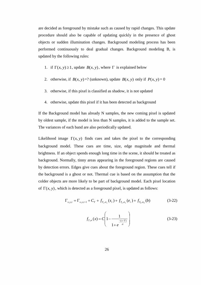
Background Updating:

Background modeling is updated for the purpose of dealing with gradual changes

like day to night changes. The objects are also placed to the background, in

following cases: If the objects remain enough time in the scene and if the objects

26

are decided as foreground by mistake such as caused by rapid changes. This update

procedure should also be capable of updating quickly in the presence of ghost

objects or sudden illumination changes. Background modeling process has been

performed continuously to deal gradual changes. Background modeling B, is

updated by the following rules:

1. if 1),( yx , update ),( yxB , where is explained below

2. otherwise, if ),( yxB =? (unknown), update ),( yxB only if ),( yxP = 0

3. otherwise, if this pixel is classified as shadow, it is not updated

4. otherwise, update this pixel if it has been detected as background

If the Background model has already N samples, the new coming pixel is updated

by oldest sample, if the model is less than N samples, it is added to the sample set.

The variances of each band are also periodically updated.

Likelihood image ),( yx finds cues and takes the pixel to the corresponding

background model. These cues are time, size, edge magnitude and thermal

brightness. If an object spends enough long time in the scene, it should be treated as

background. Normally, tinny areas appearing in the foreground regions are caused

by detection errors. Edges give cues about the foreground region. These cues tell if

the background is a ghost or not. Thermal cue is based on the assumption that the

colder objects are more likely to be part of background model. Each pixel location

of ),( yx , which is detected as a foreground pixel, is updated as follows:

)()()( ,,,1,,,, bfefsfCbbeess TrTrTTtyxtyx (3-22)

)(,

1

11)(

TxT

e

Cxf (3-23)

27

ri

r iBiIr

e

))()((1

(3-24)

where, rs is the size of foreground region which includes the pixel ),( yx , b is the

maximum thermal brightness in a 77x window around the pixel ),( yx within the

same foreground region area, TC is time constant to determine how fast static

objects will be part of the background model, C is constant to control the function

value. Gradient values corresponding to the boundaries of the detected foreground

regions and the background regions ( r is the set of these points) are calculated.

Differences of these values are accumulated to get re value. This approach is based

on [22]. The function of )(, xfT is a sigmoid function which has center point at T

and whose transition width is controlled by . Parameters of equation (3-22), are

chosen empirically.

The value of the background likelihood of the pixel which is greater than 1

( 1),( yx ), is shown as an image in Figure 3-11 (from frame 300 of sequence1 of

OTCBVS dataset). This image is constructed by using each cue given in equation

(3-22). During the 300 frames, one of the people (close to building) stands almost

first 150 frames on front of the building and the other one walks along the road. The

standing person pixels are starting to be taken into the background frames because

of time cue TC . The other person causes ghost regions behind. For these situations,

edge cues give more information. Because there exist normally no human in the

current image so value of the term )(, rT efee

in equation (3-22) increases. Tinny

areas, which are detected as a foreground, are updated because of size cue

)(, rT sfss

. The colder objects which are detected as foreground, are also updated

because of thermal cue )(, bfbbT .

28

Figure 3-11 Likelihood Image of the Non-Parametric Method

3.2.6 Non-Parametric Model: Infrared and Color Separately

The same procedure as the one described in Section 3.2.5 is applied in this method.

Anisotropic diffusion and the rough pedestrian detection module are performed on

the infrared image. Update procedure is also the same, as the one described in

Section 3.2.5.

3.2.7 Mixture of K Gaussian Model

In [19] each pixel in the background model is modeled by a mixture of K Gaussian

distributions. The probability of a pixel’s having a value of Nx at time N can be

written as:

);()(1

kN

K

k

kN xwxp

(3-25)

)()(

2

1

2

12

1

)2(

1),;();(

kkT

k xx

k

Dkkk exx

(3-26)

where kw is the weight parameter, k is the mean and 2

kk is the covariance

of the kth

component. R, G and B components are assumed to be independent. The

initial weights of the K distributions at time N are adjusted as:

29

)|(ˆ)1( 1

1

Nk

N

k

N

k xwww (3-27)

where is the learning rate and )|(ˆ 1Nk xw is 1 for the first matched Gaussian

component and 0 for the remaining part. N

kw represents weight parameter at time

N of the kth

component. The K Gaussian distributions are ordered by the value of

kkw / and the first B distributions are used for the background modeling.

b

k

kb

TwB1

minarg (3-28)

where T represents the threshold for the minimum portion of the background model.

Every new pixel value tx is checked against existing K Gaussian distributions until

a match is found. A match is defined as a pixel value within 2.5 standard deviations

of a distribution. If there is no match, the mean of the least probable distribution is

replaced with the current value and initially high variance and low prior weights are

assigned to this distribution. If there is a match to one of the components, first

matched model component will be updated as follows:

1

1 )1(

N

N

k

N

k xu (3-29)

)()()1( 1

1

1

1

2

,

2

1,

N

kN

TN

kNNkNk uxux (3-30)

where the second learning rate, is

),|( 1

N

k

N

kNx (3-31)

N

k and N

k represent mean and variance values at time N of the kth

component.

In [20], an improved version of [19] is explained. Initial estimation of Gaussian

mixture model is made up with static update equations given below:

N

kNk

N

k

N

k wxwN

ww

)|(ˆ1

11

1 (3-32)

30

)(

)|(ˆ

)|(ˆ11

1

11 N

kNN

i

ik

NkN

k

N

k x

xw

xw

(3-33)

N

k

TN

kN

N

kNN

i

ik

NkN

k

N

k xx

xw

xw

))((

)|(ˆ

)|(ˆ111

1

11

(3-34)

when the first L samples are processed, L-recent window version equations are used

as given below:

N

kNk

N

k

N

k wxwL

ww

)|(ˆ1

1

1 (3-35)

N

kN

k

NNkN

k

N

kw

xxw

L

1

111 )|(ˆ1 (3-36)

N

kN

k

TN

kN

N

kNNkN

k

N

kw

xxxw

L 1

1111 ))()(|(ˆ1 (3-37)


channels domain are shown. These images are taken from frame 300 of sequence1

of OTCBVS dataset. Sudden illumination changes occur during the sequence in

visible domain. This situation affects the model of the background in that domain.

The effect of these sudden illumination changes can be seen on the background

model, in front of the building (Figure 3-12).

31

Figure 3-12 Mean Images of Infrared, Color Intensity and Color Channels of

Mixture of Gaussian Background Method

3.3 Foreground Detection

3.3.1 Foreground Detection Based on Single Gaussian Background

Model

In [1], the squared Mahalanobis distance is used for foreground detection. For the

infrared and intensity component of visible image, foreground detection is made by

equation (3-38). For the color channels component of visible image, it is made by

(3-39)

otherwise

Zyx

yxyxI

yxD

0

),(

)),(),((1

),(

2

2

2

(3-38)

otherwise

ZxCxyxDT

0

)()(1),(21 (3-39)

Where Z represents the threshold value. Each threshold value, for either of the

infrared, the color intensity and the color channels, is set empirically. Especially in

infrared domain, it is aimed to detect whole regions of the people if it is possible.

32

For the Single Gaussian background models which are explained in Sections 3.2.2,

3.2.3 and 3.2.4, the foreground regions are extracted with the same equation given

in (3-39).

To demonstrate the results of foreground detection based on the Single Gaussian

background model, frame 803 of sequence4 of the OTCBVS dataset is chosen. The

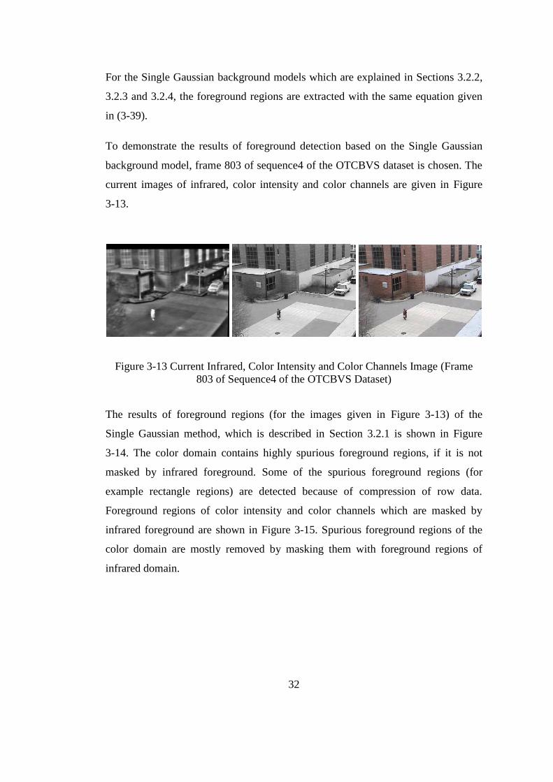
current images of infrared, color intensity and color channels are given in Figure

3-13.


803 of Sequence4 of the OTCBVS Dataset)

The results of foreground regions (for the images given in Figure 3-13) of the

Single Gaussian method, which is described in Section 3.2.1 is shown in Figure

3-14. The color domain contains highly spurious foreground regions, if it is not

masked by infrared foreground. Some of the spurious foreground regions (for

example rectangle regions) are detected because of compression of row data.

Foreground regions of color intensity and color channels which are masked by

infrared foreground are shown in Figure 3-15. Spurious foreground regions of the

color domain are mostly removed by masking them with foreground regions of

infrared domain.

33


(without Masked by Infrared Foreground)


Masked by Infrared Foreground)

In Figure 3-16, foreground regions of Single Gaussian methods which are modelled

by combinations of bands as one vector (described in Section 3.2.2, 3.2.3 and 3.2.4)

are shown. The leftmost image shows the foreground regions of the Single Gaussian

model which is constructed by infrared and color intensity modelled as one vector

(described in Section 3.2.2). The middle image shows the foreground regions of

which infrared and color channels are represented as one vector (described in

Section 3.2.3) to model the background. The rightmost image shows the foreground

regions of the model which is constructed by representing each infrared, color

intensity and color channels domain as one vector (described in Section 3.2.4). As

can be seen from the images, many spurious foreground regions are detected for all

combinations. Some of the spurious foreground regions especially in rightmost

image (for example rectangle regions) are detected because of compression of row

34

data. Trying to model each domain as one vector causes the model to be more

sensitive to noises.


Bands as One Vector)

3.3.2 Foreground Detection Based on Non-Parametric Background

Model

In [2], for a new pixel the probability that it came from the background distribution

is calculated as below:

2

2)(

2

1

1 122

11)Pr( j

jijt xxN

i

d

jj

t eN

x

(3-40)

where N and d represent the number of stored frames and used channels

respectively. d is taken 4 for this model that is L, U, V and infrared domains. 2

j

represents the variance of corresponding channels.

If the )Pr( tx of a new pixel is lower than a threshold, it is taken as a foreground

pixel. If the pixel has zero samples due to binary mask ),( yxP from the rough

pedestrian detection module, it is taken as a foreground pixel as well.

35

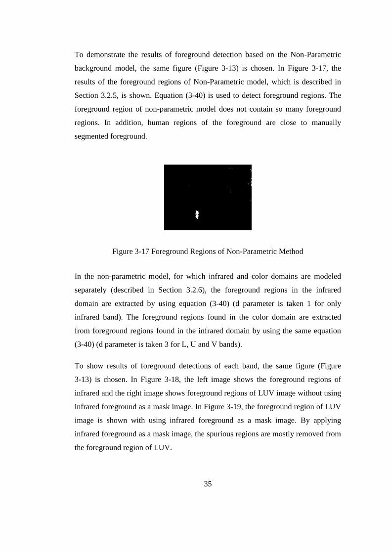
To demonstrate the results of foreground detection based on the Non-Parametric

background model, the same figure (Figure 3-13) is chosen. In Figure 3-17, the

results of the foreground regions of Non-Parametric model, which is described in

Section 3.2.5, is shown. Equation (3-40) is used to detect foreground regions. The

foreground region of non-parametric model does not contain so many foreground

regions. In addition, human regions of the foreground are close to manually

segmented foreground.

Figure 3-17 Foreground Regions of Non-Parametric Method

In the non-parametric model, for which infrared and color domains are modeled

separately (described in Section 3.2.6), the foreground regions in the infrared

domain are extracted by using equation (3-40) (d parameter is taken 1 for only

infrared band). The foreground regions found in the color domain are extracted

from foreground regions found in the infrared domain by using the same equation

(3-40) (d parameter is taken 3 for L, U and V bands).

To show results of foreground detections of each band, the same figure (Figure

3-13) is chosen. In Figure 3-18, the left image shows the foreground regions of

infrared and the right image shows foreground regions of LUV image without using

infrared foreground as a mask image. In Figure 3-19, the foreground region of LUV

image is shown with using infrared foreground as a mask image. By applying

infrared foreground as a mask image, the spurious regions are mostly removed from

the foreground region of LUV.

36


Foreground)


3.3.3 Foreground Detection Based on Mixture of Gaussian

Background Model

In [19], by considering the equation (3-28), a pixel is classified as a foreground

pixel, if it is more than 2.5 standard deviations away from any of the B distributions.

The threshold T is a measure of the minimum portion of the background model. If it

is chosen too high desired foreground regions cannot be detected. Especially in

infrared domain, it is aimed to detect whole regions of the person.


Mixture of Gaussian method, which is described in Section 3.2.7, are shown in

Figure 3-20. The color domain contains also shadow regions, if it is not masked by

infrared foreground. Foreground regions of color intensity and color channels which

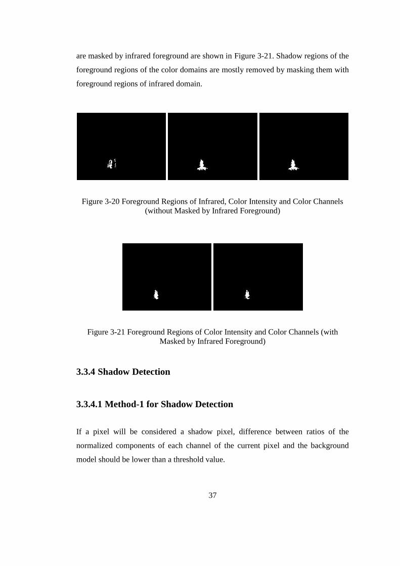
37

are masked by infrared foreground are shown in Figure 3-21. Shadow regions of the

foreground regions of the color domains are mostly removed by masking them with

foreground regions of infrared domain.


(without Masked by Infrared Foreground)


Masked by Infrared Foreground)

3.3.4 Shadow Detection

3.3.4.1 Method-1 for Shadow Detection

If a pixel will be considered a shadow pixel, difference between ratios of the

normalized components of each channel of the current pixel and the background

model should be lower than a threshold value.

38

ThBGR

BGR

BGR

BGR

bbb

bbb

ccc

ccc

,,,, (3-41)

where subscript c demonstrates the current pixel and b demonstrates the background

model of that pixel. If the above equation is hold true for each color channel

component of the pixel, it is considered as a shadow pixel.

To demonstrate the results of shadow detection algorithm, frame 319 is taken from

the sequence2 of the OTCBVS dataset which is shown in Figure 3-22.

Figure 3-22 Frame 319 of Sequence2 of the OTCBVS Dataset for Shadow

Detection

The result of method-1 for shadow detection is given in Figure 3-23. Left image

shows the result of the condition equation (3-41) and the right image shows the

masked image with the foreground region of color image. Desired shadow regions

could not be extracted by applying the equation (3-41). It is almost impossible to

eliminate shadows from the foreground regions of color image by this method. So,

it is not used in our algorithm.

39


Final Shadow Image After Masked with Foreground Region of Color Image


In [20], shadow detection is performed via comparing the current pixel chrominance

and brightness value with the corresponding background pixel values. The

computational color model expressed in [23] is used. In this model, a chromaticity

line passing through the origin is formed by using the background R, G and B

values (mean values) of each pixel location. The distortion of chromaticity line of

the current pixel values to the corresponding background model line is calculated

for that pixel. Two distortion measurements are calculated: Brightness and

chromaticity distortion. The brightness distortion measures how close the current

pixel value to the expected chromaticity line is. It is a scalar value and is calculated

by minimizing the equation given below:

2)()( iiii EI (3-42)

where iE is the expected color of the background model.

The orthogonal distance from the current chromaticity line to the background

chromaticity line is defined as the color distortion iCD and calculated as given

below:

iiii EICD (3-43)

40

After some derivations, brightness distortion and color distortion are calculated by

the equations given below;

222 ))(())(())((

)()()()()()(

iii

iiIiiIiiI

BGR

BBGGRR

i

(3-44)

222 ))()(())()(())()(( iiIiiIiiICD BiBGiGRiRi (3-45)

A pixel is considered as a shadow pixel if brightness distortion is within 2.5

standard deviation and the condition of 1 iCD is true for chromaticity

distortion iCD .

The same figure (Figure 3-22) is used to demonstrate the result of method-2. In

Figure 3-24, the left image shows the original shadow regions where conditions of

brightness and chromaticity distortion CDi are hold true. The right image shows

the masked image with foreground regions of color image. This method is not used

in our algorithm, because the shadow regions could not be differentiated from the

foreground regions of color image, as it can be seen in Figure 3-24.


Final Shadow Image After Masked with Foreground Region of Color Image

41


In [2], shadow detection is found by calculating the decrease in brightness and the

chromaticity for each pixel. Only mean values of L, U and V bands of the

background model are used for these purposes. In order a pixel p to be accepted as a

shadow pixel, all the conditions below should be satisfied:

1. 98.08.0 LC , where LLL BpC /

2. 20UVC , where 22 )()( VVuUUV pBpBC

Where LC is the change of luminance, UVC is the change of chrominance, LB , UB

and VB are the average background values of each band. These pixels are

considered as potential shadow pixels. Detected foreground regions that overlapped

with the potential shadow regions is computed and the ratio of:

F

S (3-46)

is calculated. Where, S is the area of the shadow and F is the area of the

foreground regions. Final shadow regions are found by the condition: .

and parameters limit the shadow region area with the corresponding

overlapped foreground. and parameters are set such that any of the person

regions do not considered as shadow regions.

The same figure (Figure 3-22) is used to demonstrate the result of method-3. In

Figure 3-25, left image shows possible shadow regions before the application of

condition equation (3-46) and the right image shows the result of shadow detection

after applying the equation. As it can be seen in Figure 3-25, almost whole shadow

regions are detected as possible shadow regions. Final shadow regions are extracted

42

from these possible shadow regions. This method is used in our algorithm to

remove shadow regions from the foreground regions of color domain.

Figure 3-25 Shadow Detection Results for Method-3, Possible Shadow Image and

Final Shadow Image

3.3.5 Fusion of Infrared and Visible Domains

For the background models, (described in Section 3.2.1, 3.2.6 and 3.2.7) where the

infrared and color domains are modeled separately, the fusion of the infrared and

visible domain is performed as explained below:

Pixel-wise OR operation is applied between the foreground regions of masked color

intensity and color channels. From these regions, detected shadows regions are

removed. After shadow elimination from the foreground regions of color domain,

pixel-wise OR operation is applied between these regions and the foreground

regions of the infrared. The resulting foreground regions are used as a mask in the

application of the snake algorithm.

To demonstrate the results of fusion of infrared and visible domains based on the

Single Gaussian (SG), Mixture of Gaussian (MOG) and Non-Parametric (Non-

Param) background models (described in Section 3.2.1, 3.2.6 and 3.2.7), frame 665

is taken from the sequence3 of the OTCBVS dataset which is shown in Figure 3-26.

As it can be seen from Figure 3-27, Figure 3-28 and Figure 3-29 some regions of

the people cannot be detected, furthermore the person regions are divided into at

43

least two parts in infrared domain. After the addition of the color foreground, these

regions are almost completed as seen in the rightmost image of each figure.




Resulting Final Foreground (Based on SG Background Model)


Resulting Final Foreground (Based on Non-Param Background Model)

44


Resulting Final Foreground (Based on MOG Background Model)

For the background models, (described in Section 3.2.2, 3.2.3, 3.2.4, 3.2.5) fusion

of the infrared and color domain is performed in background model. For the Single

Gaussian methods, a pixel is represented as a vector which contains each domain

and only one foreground region is extracted by applying the equation (3-39). For the

Non-Parametric method, N frames are stored for each band and only one

foreground region is extracted by applying the equation (3-40). Finally shadow

regions are removed from these foreground regions and it is used as a mask for the

application of snake algorithm.

Frame 240 is taken from the sequence4 of the OTCBVS dataset which is shown in

Figure 3-30 to demonstrate the results. In Figure 3-31, the leftmost image shows the

final foreground regions of the Single Gaussian model which is constructed by

infrared and color intensity modelled as one vector (described in Section 3.2.2). The

next image shows the final foreground regions of which infrared and color channels

domains are represented as one vector (described in Section 3.2.3) to model the

background. The next image shows the final foreground regions of the model which

is constructed by representing each infrared, color intensity and color channels

domain as one vector (described in Section 3.2.4). Rightmost image shows the final

foreground regions of Non-Parametric background model (described in Section

3.2.5).

As it can be seen from the Figure 3-31, final foreground region, which is based on

Non-Parametric background model, does not contain so many spurious and it is so

45

close to the manually segmented human region. Representing the combinations of

each band as one vector does not give desired results.



Figure 3-31 Final Foreground Regions (Combination of Bands as One Vector of

Single Gaussian and Non-Parametric Background Model)

3.4 Application of Snake Algorithm

The main goal of active contour models or snakes is to detect objects in a given

image, by evaluating a curve. In [21] Chan and Vese proposed a model which can

detect objects whose boundaries are not necessarily defined by gradient. It is based

on Mumford-Shah segmentation techniques [28] and the level set method. The

model is trying to separate the image into regions based on intensities. Starting with

a curve whose position can be anywhere in the image, the curve moves toward its

interior normal and stops on the boundary of the object. The main problem is the

minimization of energy based-segmentation.

46

To explain the main idea in a simple way, the equation (3-47) can be considered:

dxdycyxudxdycyxuCFCFCoutsideCinside

2

)(20

2

)(1021 ),(),()()( (3-47)

where C is the curve which will be evolved, ),(0 yxu is the given image and it is

assumed that two regions exist in the image which has approximately constant

intensities. 1c and 2c are the average intensity values of the inside and outside of

the C . It can be seen that the boundary of the object 0C will minimize the (3-47)

After adding some regularizing terms to (3-47), the energy function becomes:

dxdycyxudxdycyxu

CinsideAreaCLengthCccF

CoutsideCinside

2

)(202

2

)(101

21

),(),(

))(()(),,(

(3-48)

Where 0 , 0 , 121 and the problem becomes of minimization of

CccF ,, 21 with respect to 1c , 2c and C . The model is solved by level set

formulation. The contour C is represented by the zero level set of a Lipschitz

function : such that

},0),(:),{()(

},0),(:),{()(

},0),(:),{(

yxyxCoutside

yxyxCinside

yxyxC

Introducing the Heaviside function H, and the one-dimensional Dirac measure 0 ,

the terms in the energy function of F can be expressed as:

dxdyyxHA

dxdyyxyxL

,0

,,0

(3-49)

47

The intensity terms:

dxdyyxHcyxudxdycyxu

dxdyyxHcyxudxdycyxu

))),((1(),(),(

)),((),(),(

2

20

0

2

20

2

10

0

2

10

(3-50)

The average intensities 1c and 2c can be calculated as:

dxdyyxH

dxdyyxHyxu

c

dxdyyxH

dxdyyxHyxu

c

))),((1(

))),((1)(,(

)(

)),((

)),((),(

)(

0

2

0

1

(3-51)

Minimizing F function with respect to is done by Euler-Lagrange equation while

keeping 1c and 2c constant:

2

202

2

101 )()()()( cucut

(3-52)

where the curvature can be expressed as:

2/322

22

)(

2)(

yx

xyyyxxyyxx

div

(3-53)

The basic algorithm:

1. Initialization n and contour (any shape can be the initialization shape)

2. Increase n by 1

48

3. Compute the average intensities 1c and 2c of the image pixels inside and

outside (3-51)

4. Evolve the level set function (3-52)

5. Repeat the steps 2, 3 and 4 until the solution is stationary or n exceeds the

limit of iteration

The algorithm given in [24] is tried to be implemented for this purpose. This

algorithm is applied to each connected component of the foreground image

extracted from the thermal channel. To get more precise results, the area and the

center of each connected component are computed and used for the initialization of

the snake. The shape of the contour is chosen as a circular. The radius of the circle

and the iteration number of the algorithm is changed according to the area of the

connected component.

To demonstrate the results of application of snake algorithm, frame 319 is taken

from the sequence2 of the OTCBVS dataset which is shown in Figure 3-32.

Because of the halo effect around the people is weaker for this OTCBVS dataset

and the background temperature is so close to the human temperature, in the snake

algorithm, contour can not surround the boundary of the human objects as it can be

seen in Figure 3-33. In our database the halo effects that surround the people are

more evident than in OTCBVS dataset and contour could surround the boundary of

the human objects more precisely. The results of the application of snake algorithm

are also given in Section 4.4.

49




Application of Snake Algorithm

50

CHAPTER 4

EXPERIMENTAL RESULTS

In this study, various background models are implemented to get foreground

regions and proposed snake algorithm is applied to the final foreground regions in

order to detect people in two different databases. One of them is the “OSU Color-

Thermal Dataset” in OTCBVS benchmark [25] and the other one is constructed by

us. Results are demonstrated and compared against manually segmented human

regions. Our results are also compared with a previous study [1] (described in

Section 2.1).

“OSU Color-Thermal Dataset” contains six challenging thermal/color video

sequences. They are recorded from two different locations, at different times of the

day and with different camera gain and level settings. Our dataset also contains six

challenging thermal/color video sequences. Three different places are used for

recording at different times of the day and recorded with different camera gain and

level settings.

4.1 Experimental Setup

The main parts of the experimental setup are as follows:

i) A box which consists of an infrared and a visible camera: The infrared

camera, TU2, is a long wave infrared imaging camera designed for use in

the security industry. The infrared detector has the features: 320 x 240

51

pixels, Uncooled Focal Plane Array, 625 Lines (PAL/CCIR) Compliant. The

visible camera, EQ2700, is ¼” day/night camera. The specifications of the

EQ2700: PAL signal system, total pixels no. 795 (H) x 596 (V), electronic

shutter 1:50~1:10000, 1 Vp-p composite PAL, BNC, S-video mini DIN

video output, 27x optical and 10x digital zoom.

ii) Two PAL recorders (Mini-DV) to record each video stream.

iii) An interface box: It is prepared to control the parameters of both infrared

and visible camera and also provide links between PAL recorders and

cameras. For infrared camera, by using focus switch, far/near focusing is

adjusted, by using polarity switch, black/white polarity is chosen, via gain

and level button, gain and level tuning is done. For visible camera,

parameters can be changed via RS232 connection.

iv) Power supply unit to supply the cameras.

Figure 4-1 shows the components of our experimental setup and one of the

experimental setup places.

Figure 4-1 Experimental Setup and Place

Scenarios are recorded into tapes via PAL recorders. Recorded videos are captured

by using Microsoft Windows Movie Maker via IEEE1394 port. Captured frames are

52

saved using digital device format (DV-AVI). Xvid MPEG-4 codec is used to

compress saved file to save space in the storage device. The proposed algorithms

are applied to these recorded files.

4.2 Background Modelling

Background modelling methods which are described in Section 3.2 are

implemented. Some of the results are presented to compare differences of the

methods.


channels domain of the Single Gaussian method, which is described in Section

3.2.1, are shown. The results of the Mixture of Gaussian which is described in

Section 3.2.7, is also given in Figure 4-3. These images are taken from frame 300 of

scene3 of our dataset. One person walks through the road and gets out of the sight

of the cameras during the frame 300. The path followed by the person can be seen

on the mean image of the color channels based on the Single Gaussian method (in

Figure 4-2). Whereas the mean image of the color channels, which is based on the

Mixture of Gaussian background model, does not include this path and it is

modelled more correctly.



53

Figure 4-3 Mean Images of Infrared, Color Intensity and Color Channels of Mixture


4.3 Foreground Detection

In this part, detected foreground regions for each background model is presented.

The foreground detection algorithms are explained in Section 3.3.

To demonstrate the foreground regions for all background modelling methods from

our dataset, the current images of infrared, color intensity and color channels which

are shown in Figure 4-4, are taken from frame 373 of scene2 of our dataset.

Figure 4-4 Current Infrared, Color Intensity and Color Channels Image (Frame 373

of Scene2 of Our Dataset)

The results of foreground regions (for the images given in Figure 4-4) of the Single

Gaussian method, which is described in Section 3.2.1 is shown in Figure 4-5. In our

dataset, the halo effects around the people are more evident than OTCBVS dataset.

54

The color domain contains highly spurious foreground regions, if it is not masked

by infrared foreground. Some of the spurious foreground regions (for example

rectangle regions) are detected because of compression of row data. Foreground

regions of color intensity and color channels which are masked by infrared

foreground are shown in Figure 4-7. Spurious regions of the foreground regions of

the color domains are mostly removed by masking them with foreground regions of

infrared domain.


(without Masked by Infrared Foreground) Based on Single Gaussian Background

Model


Masked by Infrared Foreground) Based on Single Gaussian Background Model


Mixture of Gaussian method, which is described in Section 3.2.7, are shown in

Figure 4-7. The color domain contains spurious foreground regions and also shadow

regions. Spurious foreground regions are reduced compared with Single Gaussian

55

method (Figure 4-7). They are mostly removed by masking them with infrared

foreground. The results are shown in Figure 4-8.


(without Masked by Infrared Foreground) Based on Mixture of Gaussian

Background Model


Masked by Infrared Foreground) Based on Mixture of Gaussian Background Model

In Figure 4-9, the results of the foreground regions of Non-Parametric model with

IR and L, U, V bands used separately which is described in Section 3.2.6, are

shown. Left image shows foreground regions of infrared and the right image shows

foreground regions of LUV image without using infrared foreground as a mask

image. By applying infrared foreground as a mask image to the foreground regions

of LUV image, the spurious regions are mostly removed (see Figure 4-10).

Silhouette of the person is more evident for foreground region of color domain in

this model compared with Single Gaussian and Mixture of Gaussian background

models.

56


Foreground) Based on Non-Parametric Method


Based on Non-Parametric Method

In Figure 4-11, the results of the foreground regions of Non-Parametric model

which is described in Section 3.2.5, are shown. The foreground region of non-

parametric model does not contain so many spurious foreground regions. In

addition, human regions of the foreground are close to the manually segmented

human regions.

57

Figure 4-11 Foreground Regions of Non-Parametric Method

In Figure 4-12, foreground regions of Single Gaussian methods which are modelled

by combinations of bands as one vector (described in Section 3.2.2, 3.2.3 and 3.2.4)

are shown. The leftmost image shows the foreground regions of the Single Gaussian

model which is constructed by infrared and color intensity modelled as one vector

(described in Section 3.2.2). The middle image shows the foreground regions of

which infrared and color channels domains are represented as one vector to model

the background (described in Section 3.2.3). The rightmost image shows the

foreground regions of the model which is constructed by representing each infrared,

color intensity and color channels domain as one vector (described in Section

3.2.4). As can be seen from the images, many spurious regions are detected for all

combinations. Some of the spurious foreground regions especially in middle and

rightmost image (for example rectangle regions) are detected because of

compression of row data.


Bands as One Vector)

58

4.3.1 Fusion of Infrared and Visible Domain

When the temperature of an object and its surrounding area is closer, detection of

the object from thermal image becomes more difficult. In these situations, if the

colors of the object and the background are not similar and illumination is available,

visual spectrum cameras give more cues that can be used to detect the object. This

situation is illustrated in Figure 4-14. The leftmost image shows the foreground

detection in infrared domain without the addition of foreground in the visible

domain. As can be seen in the image, some regions of the people cannot be

detected, furthermore the person regions are divided into at least two parts. The

middle image shows the foreground regions of color domain. After the addition of

the visible cues, these regions are almost completed as seen in the rightmost image

in Figure 4-14. This completion procedure is described in Section 3.3.5. These

images are taken from the results of foreground regions based on Single Gaussian

background modeling (described in Section 3.2.1) and frame 1721 of scene3 is used

from our database.


Visible Domain

59

Figure 4-14 Completion of Infrared Foreground Regions, Foreground Region of

Infrared, Color Domain and Resulting Final Foreground

4.4 Application of Snake

To demonstrate the results of application of snake algorithm (described in Section

3.4), frame 1400 is taken from the scene4 of our dataset which is shown in Figure

4-15. One of the examples of the application of snake algorithm is illustrated in

Figure 4-16. The leftmost image shows the detected foreground regions of the

infrared image including the objects (people) and the halo effects around them. The

middle image shows the constructed final foreground region. The snake algorithm is

applied to each connected component of the image which is formed by masking the

infrared image by the constructed foreground mask. The result of the snake

algorithm is shown in the rightmost image of Figure 4-16. Here, people are

segmented and the boundaries of people are very clear.


Visible Domain

60


Application of Snake Algorithm

4.5 Performance for the Whole Algorithm

To measure the performance of our algorithm and to compare the results with the

results given in [1], the human regions of the 60 image pairs from the “OSU Color-

Thermal Dataset” in OTCBVS benchmark (10 frames for each sequence) are

manually segmented. All the parameters and threshold values are fixed to present

the applicability of the proposed algorithm for various sequences. Different

background models are used to demonstrate the affects of background model to the

results.

The performance is also presented by Recall (R) (Sensitivity), Precision (P)

(Positive Predictive Value) and F-measure values (described in [1]). Recall

indicates the ratio of object pixels that the algorithm has found correctly over

actually manually segmented region. Precision indicates the ratio of object pixels

that the algorithm has found correctly over in fact object regions. F-measure is a

harmonic mean of the precision and the recall value.

Let S(A) represents the area of the object pixels that the algorithm has found

correctly and let S(B) represents the area of the object pixels that manually

segmented.

Recall value is calculated as:

)(

)(

BS

BAS (4-1)

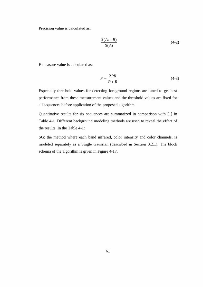
61

Precision value is calculated as:

)(

)(

AS

BAS (4-2)

F-measure value is calculated as:

RP

PRF

2 (4-3)

Especially threshold values for detecting foreground regions are tuned to get best

performance from these measurement values and the threshold values are fixed for

all sequences before application of the proposed algorithm.

Quantitative results for six sequences are summarized in comparison with [1] in

Table 4-1. Different background modeling methods are used to reveal the effect of

the results. In the Table 4-1:

SG: the method where each band infrared, color intensity and color channels, is

modeled separately as a Single Gaussian (described in Section 3.2.1). The block

schema of the algorithm is given in Figure 4-17.

62

Figure 4-17 The Block Schema of the Algorithm Based on SG and MOG

Background Models

MOG: the method where each band, infrared, color intensity and color channels, is

modeled separately as a Mixture of Gaussian (described in Section 3.2.7). The

block schema of the algorithm is given in Figure 4-17.

Non-Param-1: the method where each band, infrared and color domains, is modeled

separately as a Non Parametric (described in Section 3.2.6). The block schema of

the algorithm is given in Figure 4-18.

63

Figure 4-18 The Block Schema of the Algorithm Based on Non-Param-1

Background Model

Non-Param-2: the method where each band is modeled as a Non Parametric in the

background model by storing N frames (described in Section 3.2.5). The block

schema of the algorithm is given in Figure 4-19.

Figure 4-19 . The Block Schema of the Algorithm Based on Non-Param-2

Background Model

In all sequences, for our algorithm, recall values are higher but the precision values

are smaller than the ones expressed in [1]. This means that more actual regions are

detected. And the main reason of smaller precision is the weakness of the halo

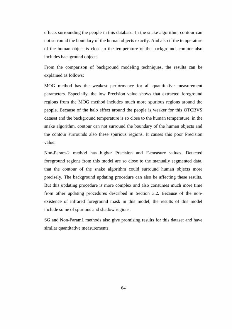
64

effects surrounding the people in this database. In the snake algorithm, contour can

not surround the boundary of the human objects exactly. And also if the temperature

of the human object is close to the temperature of the background, contour also

includes background objects.

From the comparison of background modeling techniques, the results can be

explained as follows:

MOG method has the weakest performance for all quantitative measurement

parameters. Especially, the low Precision value shows that extracted foreground

regions from the MOG method includes much more spurious regions around the

people. Because of the halo effect around the people is weaker for this OTCBVS

dataset and the background temperature is so close to the human temperature, in the

snake algorithm, contour can not surround the boundary of the human objects and

the contour surrounds also these spurious regions. It causes this poor Precision

value.

Non-Param-2 method has higher Precision and F-measure values. Detected

foreground regions from this model are so close to the manually segmented data,

that the contour of the snake algorithm could surround human objects more

precisely. The background updating procedure can also be affecting these results.

But this updating procedure is more complex and also consumes much more time

from other updating procedures described in Section 3.2. Because of the non-

existence of infrared foreground mask in this model, the results of this model

include some of spurious and shadow regions.

SG and Non-Param1 methods also give promising results for this dataset and have

similar quantitative measurements.

65

Table 4-1 Comparison of Results: Our Algorithm (Based on Kinds of Background

Modelling) and Reference [1]

Sequences SG MOG Non

Param-1

Non

Param-2 In [1]

Seq1

Recall 0.731 0.793 0.786 0.753 0.714

Precision 0.722 0.564 0.659 0.712 0.914

F-Measure 0.726 0.659 0.717 0.732 0.802

Seq2

Recall 0.811 0.705 0.786 0.800 0.719

Precision 0.722 0.658 0.731 0.770 0.874

F-Measure 0.764 0.680 0.757 0.785 0.789

Seq3

Recall 0.748 0.776 0.753 0.767 0.655

Precision 0.915 0.822 0.822 0.879 0.905

F-Measure 0.823 0.799 0.786 0.819 0.760

Seq4

Recall 0.912 0.894 0.834 0.892 0.734

Precision 0.747 0.660 0.842 0.921 0.955

F-Measure 0.821 0.760 0.838 0.907 0.830

Seq5

Recall 0.915 0.587 0.873 0.900 0.809

Precision 0.705 0.612 0.822 0.905 0.957

F-Measure 0.796 0.599 0.847 0.902 0.877

Seq6

Recall 0.962 0.939 0.922 0.954 0.780

Precision 0.569 0.412 0.697 0.814 0.931

F-Measure 0.715 0.573 0.847 0.878 0.851

Overall

Recall 0.846 0.782 0.826 0.844 0.722

Precision 0.730 0.621 0.762 0.833 0.916

F-Measure 0.784 0.693 0.793 0.839 0.808

The results from each sequence are visualized below where the first row includes

from left to right the tested images of infrared, color intensity, color channels and

manually segmented human regions. The second row shows the output of the

proposed algorithm. In the second row, leftmost image is based on SG method, the

next image is based on MOG method, the next one is based on Non-Param-1

method and the rightmost image is based on Non-Param-2 method.

66

Figure 4-20 Results from Frame 652 of Sequence1 of OTCBVS Dataset


67



68

Figure 4-24 Results from Frame 508 of Sequence5 in OTCBVS Dataset

Figure 4-25 Results from Frame 820 of Sequence6 in OTCBVS Dataset

The results of our algorithm when Single Gaussian method is used for background

modelling (described in Section 3.2.2, 3.2.3 and 3.2.4) where combinations of each

band are represented as one vector, is shown as on a single sequence. The reason of

for this is that highly spurious foreground regions are detected when this

background modelling is used.

69

The results are presented in Table 4-2. Where SG-1 stands for a background model

where infrared and color intensity domains are expressed as one vector (described

in Section 3.2.2). SG-2 stands for a background model where infrared and color

channels domains are expressed as one vector (described in Section 3.2.3). SG-3

stands for a background model where infrared and color intensity and color

channels domains are expressed as one vector (described in Section 3.2.4). SG-4

stands for a background model where infrared and color channels (L, U and V

bands) are expressed as one vector. The block schema of the algorithm is given in

Figure 4-26. For the SG-4 model, the color conversion is performed RGB to LUV

before processing the color image.

Figure 4-26 The Block Schema of the Algorithm Based on Single Gaussian where

Combinations of each band is modelled as One Vector

Although SG-1 has the weakest performance for Precision and F-measure value, it

has the maximum Recall value and minimum spurious regions compared to the

other two methods. Most spurious regions are detected from the SG3 and this model

is the most sensitive model to noises. Foreground regions for all four methods

include highly spurious regions around the people. Contour can not surround the

boundary of the human objects and it surrounds also these spurious regions. So, it

causes this poor Precision value for these methods.

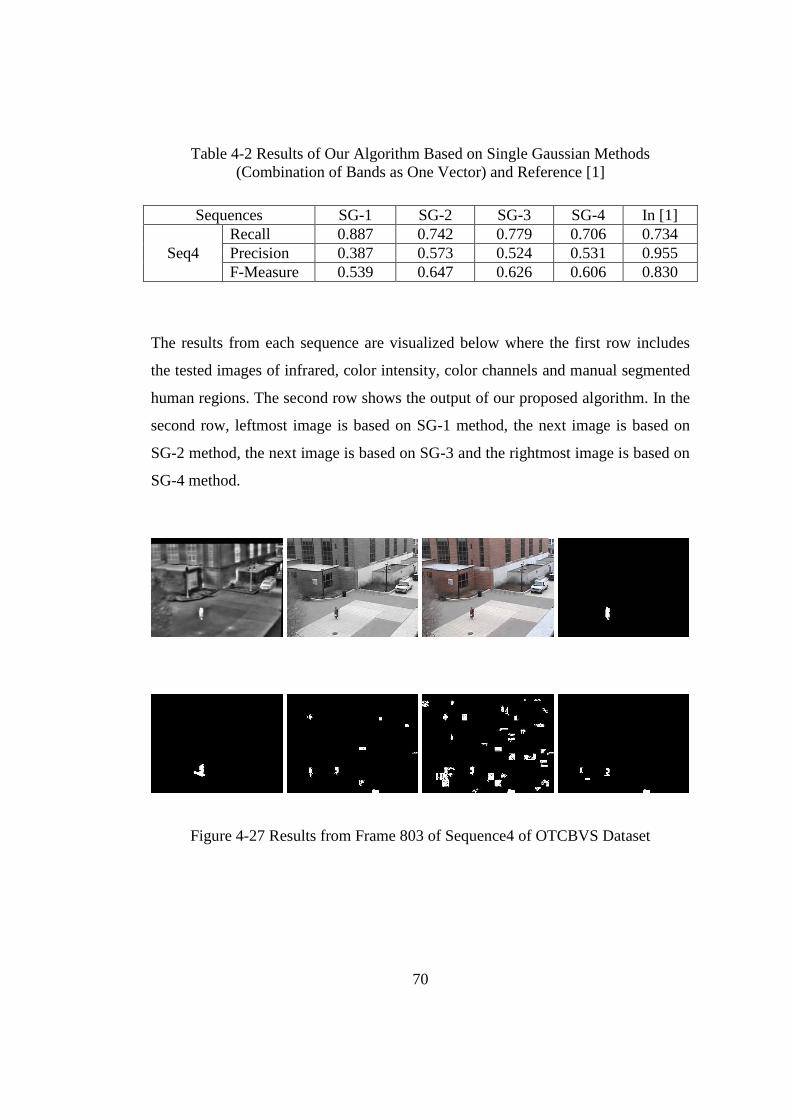
70

Table 4-2 Results of Our Algorithm Based on Single Gaussian Methods

(Combination of Bands as One Vector) and Reference [1]

Sequences SG-1 SG-2 SG-3 SG-4 In [1]

Seq4

Recall 0.887 0.742 0.779 0.706 0.734

Precision 0.387 0.573 0.524 0.531 0.955

F-Measure 0.539 0.647 0.626 0.606 0.830


the tested images of infrared, color intensity, color channels and manual segmented

human regions. The second row shows the output of our proposed algorithm. In the

second row, leftmost image is based on SG-1 method, the next image is based on

SG-2 method, the next image is based on SG-3 and the rightmost image is based on

SG-4 method.


71

Our database is also used to measure the performance of our proposed algorithm. In

our database the halo effects that surround the people are more evident than in

OTCBVS dataset. From each sequence, 10 frames are selected and compared with

the manually segmented regions. Quantitative results are given in Table 4-3 for our

database. All of the parameters and threshold values are fixed to present the

applicability of the proposed algorithm for various sequences. Different background

models are used to demonstrate the effects of background modelling to the results.

In our dataset, the performance of the algorithm is also demonstrated when only

infrared domain is used based on Single Gaussian background model. SG-Only IR

the method where infrared band is modeled as a Single Gaussian. The block schema

of the algorithm is given in Figure 4-28.

Figure 4-28 The Block Schema of the Algorithm Based on SG-IR where Only

Infrared Band is Used

Since the halo effects surrounding people are more evident in our dataset, high

performance can be obtained. Overall Recall value is greater than or equal to 0.95

for all background models (except SG-Only IR) which shows that our algorithm

covers almost all manually segmented human regions. Precision values is greater

than 0.875 for all background models (except Non-Param1) which shows that

detected object from our algorithm is not scattered so much around the manually

segmented human regions. For the Non-Param1 method, in some of the frames

(Figure 4-33), two people are extracted as one connected component. It decreases

the overall Precision value of this model. For the SG-Only IR method, because of

only infrared domain is used, there exist no cues available to complete missing parts

of the regions of the people (Figure 4-29). It causes low overall recall value for the

model.

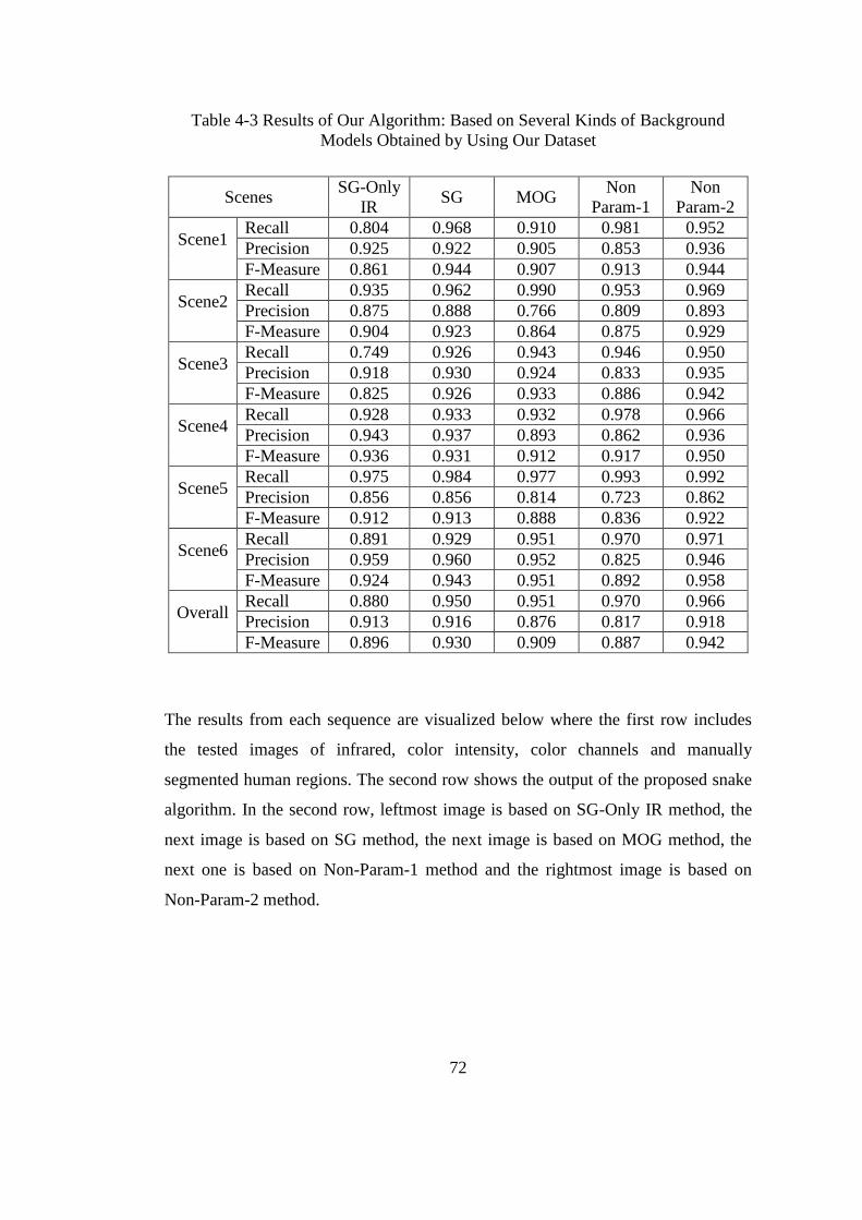
72

Table 4-3 Results of Our Algorithm: Based on Several Kinds of Background

Models Obtained by Using Our Dataset

Scenes SG-Only

IR SG MOG

Non

Param-1

Non

Param-2

Scene1 Recall 0.804 0.968 0.910 0.981 0.952

Precision 0.925 0.922 0.905 0.853 0.936

F-Measure 0.861 0.944 0.907 0.913 0.944

Scene2 Recall 0.935 0.962 0.990 0.953 0.969

Precision 0.875 0.888 0.766 0.809 0.893

F-Measure 0.904 0.923 0.864 0.875 0.929

Scene3 Recall 0.749 0.926 0.943 0.946 0.950

Precision 0.918 0.930 0.924 0.833 0.935

F-Measure 0.825 0.926 0.933 0.886 0.942

Scene4 Recall 0.928 0.933 0.932 0.978 0.966

Precision 0.943 0.937 0.893 0.862 0.936

F-Measure 0.936 0.931 0.912 0.917 0.950

Scene5 Recall 0.975 0.984 0.977 0.993 0.992

Precision 0.856 0.856 0.814 0.723 0.862

F-Measure 0.912 0.913 0.888 0.836 0.922

Scene6 Recall 0.891 0.929 0.951 0.970 0.971

Precision 0.959 0.960 0.952 0.825 0.946

F-Measure 0.924 0.943 0.951 0.892 0.958

Overall Recall 0.880 0.950 0.951 0.970 0.966

Precision 0.913 0.916 0.876 0.817 0.918

F-Measure 0.896 0.930 0.909 0.887 0.942


the tested images of infrared, color intensity, color channels and manually

segmented human regions. The second row shows the output of the proposed snake

algorithm. In the second row, leftmost image is based on SG-Only IR method, the

next image is based on SG method, the next image is based on MOG method, the

next one is based on Non-Param-1 method and the rightmost image is based on

Non-Param-2 method.

73

Figure 4-29 Results from Frame 1656 of Scene1 of Our Dataset



74




75

The results of our method when Single Gaussian background modelling is used

where combinations of each band are represented as one vector, is shown only for a

single sequence in Table 4-4. The reason of this is that highly spurious foreground

regions are detected for these methods. The results based on the SG-1 model have

the least spurious object and this model has highest Precision value compared to

other three methods for our dataset. SG-2, SG3 and SG-4 model have higher

spurious foreground regions and this affects the results as can be seen from the

Table 4-4.

Table 4-4 Results of Based on Single Gaussian Methods (Combination of Bands as

One Vector) Obtained by Using Our Dataset

Scenes SG-1 SG-2 SG-3 SG-4

Scene2

Recall 0.645 0.727 0.607 0.764

Precision 0.750 0.419 0.633 0.713

F-Measure 0.693 0.532 0.620 0.738


the tested images of infrared, color intensity, color channels and manual segmented

human regions. The second row shows the output of our proposed algorithm. In the

second row, leftmost image is based on SG-1 method, the next image is based on

SG-2 method, the next image is based on SG-3 and the rightmost image is based on

SG-4 method.

76


77

CHAPTER 5

SUMMARY AND CONCLUSIONS

In this thesis, detection of foreground objects, especially people, is performed

using synchronized and registered infrared and visual images all together.

Sudden illumination changes and shadows do not generally affect the

background model in infrared domain. The temperature of the background is

more stable over time and operation of all around the day is valid in infrared

domain. These are the main reasons that the initial regions of interest are found

firstly in infrared domain and these regions are used as a mask in the visible

domain. However, some object regions may not be detected from infrared image

due to the fact that the temperature of the foreground objects may be very close

to the background model. Thus, after finding the corresponding foreground

regions in visible domain, addition of the visible cues (if available) to foreground

regions of infrared domain is performed. As a result, the missing regions are

complete on the thermal foreground mask using corresponding visual

information. Finally, application of snake algorithm to the current infrared

image, which is masked with the constructed foreground regions, gives very

successful results for people detection. Results are more robust when the halo

effects surrounding the people are more evident.

Performance of the proposed algorithm is tested with two datasets (OTCBVS

benchmark and our dataset) each of which includes six challenging sequences.

For each sequence, 10 frames are chosen and segmented manually. To show

applicability of our algorithm for various sequences, all parameters/thresholds

78

are fixed before tests. The quantitative performance is demonstrated by precision

and recall parameters. The results are compared also with the results given in [1]

by using the OTCBVS benchmark. Although these sequences have weaker halo

effects which surround the people, promising results are derived. In all sequences

our recall values are higher but the precision values are smaller than the ones

expressed in [1]. This means that we detect more of the actual regions. In our

dataset, halo effects are more evident and in these sequences we obtain better

results. Various background modeling methods have been used for this purpose.

Effects of these methods to human detection performance are also given in

Section 4.5.

Object identification will be the topic of future research. For example, some

basic parameters like area of the blob, height to width ratio etc. will be used to

eliminate non-human objects. If clear human silhouettes could be extracted,

further tasks such as activity recognition could also be studied.

79

REFERENCES

[1]: J. W. Davis, and V. Sharma. “Background-subtraction using contour-based

fusion of thermal and visible imagery”. In Computer Vision and Image

Understanding 106(2-3): 162-182, 2007.

[2]: C. O. Conaire, E. Cooke, N. O’Connor, N. Murphy, and A. Smeaton.

“Background modelling in infrared and visible spectrum video for people tracking”.

In Proc. IEEE Conf. on Computer Vision and Pattern Recognition Workshop,page

20, Washington, DC, USA, 2005.

[3]: A. Elgammal, D. Harwood, and L. Davis. “Non-parametric model for

background subtraction”. In Proceedings of the 6th

European Conference on

Computer Vision, 2000.

[4]: A. Leykin, Y. Ran, and R. Hammoud, “Thermal-visible video fusion for

moving target tracking and pedestrian classification”. In Computer Vision and

Pattern Recognition, 2007. CVPR '07. IEEE Conference on 17-22 June 2007

Page(s):1 - 8

[5]: K. Kim, T. H. Chalidabhongse, D. Harwood, and L. Davis. “Background

modeling and subtraction by codebook construction”. In International Conference

on Image Processing, 2004.

[6]: A. Leykin and M. Tuceryan. “A vision system for automated customer tracking

for marketing analysis: Low level feature extraction”. In Human Activity

Recognition and Modelling Workshop, 2005.

80

[7]: Y Ran, I. Weiss, Q. Zheng, and L. S. Davis: “Pedestrian detection via periodic

motion analysis”. In International Journal of Computer Vision 71(2): 143-160

(2007)

[8]: I. Haritaoglu, D. Harwood, and L.S. Davis, “W4: real-time surveillance of

people and their activities”. In IEEE Transactions on Pattern Analysis and Machine

Intelligence, Vol. 22, No. 8, pp. 809-830, 2000.

[9]: L. Zhang, B. Wu, and R. Nevatia. “Pedestrian detection in infrared images

based on local shape features”. In the 4-th Joint IEEE International Workshop on

Object Tracking and Classification in and Beyond the Visible Spectrum

(OTCBVS'07), in conjunction with CVPR 2007

[10]: N. Dalal and B. Triggs. “Histograms of oriented gradients for human

detection”. In Coference on Computer Vision and Pattern Recognition (CVPR),

2005.

[11]: C. Dai, Y. Zheng, and X. Li. “Layered representation for pedestrian detection

and tracking in infrared imagery”. In IEEE CVPR WS on OTCBVS, 2005.

[12]: J. Zhou and J. Hoang. “Real time robust human detection and tracking

system”. In IEEE Computer Society Conference on Computer Vision and Pattern

Recognition, 3:149 – 149, 2005.

[13]: M. Hussein, W. Abd-Almageed, Y. Ran, and L. Davis: “Real-time human

detection, tracking, and verification in uncontrolled camera motion environments”.

In International Conference on Computer Vision Systems ICVS 2006

[14]: G. Wolberg and S. Zokai. “Robust image registration using log-polar

transform”. In International Conference on Image Processing, 2000.

[15]: D. Gavrila. “Pedestrian detection from a moving vehicle.”. In ECCV ’00:

Proceedings of the 6th European Conference on Computer Vision-Part II, pages

37–49, London, UK, 2000. Springer-Verlag.

81

[16]: S. K. Zhou, R. Chellappa, and B. Moghaddam. “Visual tracking and

recognition using appearance-adaptive model in particle filters”. In IEEE

Transactions on Image Processing, 13(11):1491–1506, November 2004.

[17]: R. Fletcher (Ed.), “Practical Methods of Optimization”, Wiley, New York,

1990.

[18]: H. G. Barrow. “Parametric correspondence and chamfer matching: two new

techniques for image matching.”. In International Joint Conference on Artificial

Intelligence, pages 659–663, 1977.

[19]: W. E. L. Grimson and C. Stauffer, “Adaptive background mixture models for

real-time tracking.”. In Proc. IEEE Conf. CVPR, Vol. 1, pp 22-29, 1999.

[20]: P. KadewTraKuPong and R. Bowden, "An improved adaptive background

mixture model for real-time tracking with shadow detection". In Proc. 2nd

European Workshp on Advanced Video-Based Surveillance Systems, 2001

[21]: T. Chan and L. Vese, “Active contours without edges.”. In IEEE Trans.

ImageProcessing, 10(2):266–277, Feb. 2001.

[22]: O. Javed, K. Shafique, and M. Shah. “A hierarchical approach to robust

background subtraction using color and gradient information.”. In Workshop on

Motion and Video Computing, pages 22-27, Dec 2002

[23]: T. Horprasert, D. Harwood, and L.S. Davis “A statistical approach for real-

time robust background subtraction and shadow detection.”. In IEEE ICCV'99

FRAME-RATE WORKSHOP. 1999.

[24]: http://www.engr.uconn.edu/~cmli

[25]: http://www.cse.ohio-state.edu/otcbvs-bench

http://www.engr.uconn.edu/~cmli

http://www.cse.ohio-state.edu/otcbvs-bench

82

[26]: J. Davis and V. Sharma. “Robust background-subtraction for person detection

in thermal imagery”. In IEEE International Workshop on Object Tracking and

Classification Beyond the Visible Spectrum, 2004.

[27]: J. Davis and V. Sharma. “Robust detection of people in thermal imagery”. In:

Proceedings on International Conference on Pattern Recognition, 2004, pp. 713–

716.

[28]: D. Mumford and J. Shah. “Optimal approximation by piecewise smooth

functions and associated variational problems” In Commun. Pure Appl. Math, vol.

42, pp. 577–685, 1989

[29]: N. Oliver, B. Rosario, and A. Pentland. “A Bayesian Computer Vision System

for Modeling Human Interactions”. In International Conference on Vision Systems,

1999.

[30]: Y.L.Tian and A.Hampapur. “Robust Salient Motion Detection with Complex

Background for Real-time Video Surveillance”, In Proc. Of IEEE Computer Society

Workshop on Motion and Video Computing, January, 2005

object detection from registered visual and …etd.lib.metu.edu.tr/upload/12609671/index.pdf ·...

Documents