designofmovingtargetindicationfilterswithnon …etd.lib.metu.edu.tr/upload/12615361/index.pdf ·...

DESIGN OF MOVING TARGET INDICATION FILTERS WITH NON-UNIFORM PULSEREPETITION INTERVALS

A THESIS SUBMITTED TOTHE GRADUATE SCHOOL OF NATURAL AND APPLIED SCIENCES

OFMIDDLE EAST TECHNICAL UNIVERSITY

BY

MEHMET İSPİR

IN PARTIAL FULFILLMENT OF THE REQUIREMENTSFOR

THE DEGREE OF MASTER OF SCIENCEIN

ELECTRICAL AND ELECTRONICS ENGINEERING

JANUARY 2013

Approval of the thesis:

DESIGN OF MOVING TARGET INDICATION FILTERS WITHNON-UNIFORM PULSE REPETITION INTERVALS

submitted by MEHMET İSPİR in partial fulfillment of the requirements for the degree ofMaster of Science in Electrical and Electronics Engineering Department, MiddleEast Technical University by,

Prof. Dr. Canan ÖzgenDean, Graduate School of Natural and Applied Sciences

Prof. Dr. İsmet ErkmenHead of Department, Electrical and Electronics Engineering

Assoc. Prof. Dr. Çağatay CandanSupervisor, Electrical and Electronics Engineering Dept., METU

Examining Committee Members:

Prof. Dr. Tolga ÇiloğluElectrical and Electronics Engineering Dept., METU

Assoc. Prof. Dr. Çağatay CandanElectrical and Electronics Engineering Dept., METU

Assoc. Prof. Dr. Ali Özgür YılmazElectrical and Electronics Engineering Dept., METU

Assist. Prof. Dr. Umut OrgunerElectrical and Electronics Engineering Dept., METU

Dr. Alper YıldırımChief Researcher, TÜBİTAK BİLGEM İLTAREN

Date:

I hereby declare that all information in this document has been obtained andpresented in accordance with academic rules and ethical conduct. I also declarethat, as required by these rules and conduct, I have fully cited and referenced allmaterial and results that are not original to this work.

Name, Last Name: MEHMET İSPİR

Signature :

iv

ABSTRACT

DESIGN OF MOVING TARGET INDICATION FILTERS WITH NON-UNIFORM PULSEREPETITION INTERVALS

İspir, Mehmet

M.Sc., Department of Electrical and Electronics Engineering

Supervisor : Assoc. Prof. Dr. Çağatay Candan

January 2013, 102 pages

Staggering the pulse repetititon intervals is a widely used solution to alleviate the blind speedproblem in Moving Target Indication (MTI) radar systems. It is possible to increase the firstblind speed on the order of ten folds with the use of non-uniform sampling. Improvement inblind speed results in passband fluctuations that may degregade the detection performancefor particular Doppler frequencies. Therefore, it is important to design MTI filters withnon-uniform interpulse periods that have minimum passband ripples with sufficient clutterattenuation along with good range and blind velocity performance.

In this thesis work, the design of MTI filters with non-uniform interpulse periods is studiedthrough the least square, convex and min-max filter design methodologies. A trade-off betweenthe contradictory objectives of maximum clutter suppression and minimum desired signalattenuation is established by the introduction of a weight factor into the designs. The weightfactor enables the adaptation of MTI filter to different operational scenarios such as theoperation under low, medium or high clutter power.

The performances of the studied designs are investigated by comparing the frequency responsecharacteristics and the average signal-to-clutter suppression capabilities of the filters with re-spect to a number of defined performance measures. Two further approaches are considered toincrease the signal-to-clutter suppression performance. First approach is based on a modifiedmin-max filter design whereas the second one focuses on the multiple filter implementations.In addition, a detailed review and performance comparison with the non-uniform MTI filterdesigns from the literature are also given.

v

Keywords: MTI Radar, Non-uniform PRF, Non-uniform Filtering, Clutter Suppression, BlindSpeed

vi

ÖZ

DÜZENSİZ DARBE TEKRARLAMA ARALIKLARINA SAHİP HAREKETLİ HEDEFBELİRTİSİ SÜZGEÇLERİ TASARIMI

İspir, Mehmet

Yüksek Lisans, Elektrik Elektronik Mühendisliği Bölümü

Tez Yöneticisi : Doç. Dr. Çağatay Candan

Ocak 2013, 102 sayfa

Darbe tekrarlama aralıklarını değiştirmek, Hareketli Hedef Belirtisi (MTI) radar sistemlerindekör hız problemini azaltmak için yaygın olarak kullanılan bir çözümdür. Düzgün olmayanörnekleme ile ilk kör hızın yaklaşık olarak on kat artırılması mümkündür. Kör hızdaki iyileşme,belirli Doppler frekanslarındaki tespit performansını azaltabilecek geçirme kuşağı salınımlarınaneden olmaktadır. Bu nedenle en küçük geçirme kuşağı dalgalanmasına sahip ve yeterli kargaşabastırımının yanında, iyi mesafe ve kör hız performansı olan, değişken aralıklı MTI süzgeçtasarımı önemlidir.

Bu tez çalışmasında, değişken aralıklı MTI süzgeç tasarımı en küçük kareler, konveks ve enküçük-en büyük süzgeç tasarımı metodolojileri kullanılarak çalışılmıştır. Tasarımlara ağırlıkfaktörü eklenmesi ile, çakışan en büyük kargaşa bastırımı ve en küçük istenen sinyal bastırımıamaçları arasında ilişki oluşturulmuştur. Ağırlık faktörü MTI süzgecinin düşük, orta ve yüksekgüçlü kargaşa ortamlarında işleyiş gibi farklı operasyonel senaryolara adaptasyonuna olanaksağlamaktadır.

Çalışılan tasarımların performansları, süzgeçlerin frekans cevap karakteristikleri ve ortalamasinyal-kargaşa bastırımı yetenekleri tanımlanan birkaç performans ölçütüne göre karşılaştırılarakincelenmiştir. Sinyal-kargaşa bastırımını artırmak için ilaveten iki yaklaşım değerlendirilmiştir.İlk yaklaşım değiştirilmiş en küçük-en büyük süzgeç tasarımına dayanmakta iken, ikincisiise önerilen süzgeç tasarımlarının çoklu süzgeçler olarak uygulamasına odaklanmaktadır. Ekolarak, literatürdeki düzensiz MTI süzgeç tasarımları ile de detaylı bir gözden geçirme veperformans karşılaştırması verilmiştir.

vii

Anahtar Kelimeler: MTI Radar, Düzensiz DTF, Düzensiz Süzgeçleme, Kargaşa Bastırımı, KörHız

viii

To My Family

ix

ACKNOWLEDGMENTS

By the completion of this thesis work, I have the opportunity to express my sincere gratitudesto several people for their support and guidance.

I am truly indebted and thankful to my supervisor Assoc. Prof. Dr. Çağatay Candan forhis valuable suggestions, criticism and guidance throughout the thesis work. The theoreticaldiscussions with him was very informative and guided me to the right direction all the time.He always allocated time to clarify my questions and doubts, despite his busy schedules. I feelvery lucky to find the chance to work with him for my Master’s degree.

I would like to thank my family for their constant encouragement and support.

I also wish to thank to my colleques at TÜBİTAK BİLGEM İLTAREN for their help andkindness. I gained a lot from their inputs and experience.

x

TABLE OF CONTENTS

ABSTRACT . . . . . . . . . . . . . . . . . . . . . . . . . . . . . . . . . . . . . . . . . . v

ÖZ . . . . . . . . . . . . . . . . . . . . . . . . . . . . . . . . . . . . . . . . . . . . . . . . vii

ACKNOWLEDGMENTS . . . . . . . . . . . . . . . . . . . . . . . . . . . . . . . . . . . x

TABLE OF CONTENTS . . . . . . . . . . . . . . . . . . . . . . . . . . . . . . . . . . . xi

LIST OF TABLES . . . . . . . . . . . . . . . . . . . . . . . . . . . . . . . . . . . . . . . xiii

LIST OF FIGURES . . . . . . . . . . . . . . . . . . . . . . . . . . . . . . . . . . . . . . xv

CHAPTERS

1 INTRODUCTION . . . . . . . . . . . . . . . . . . . . . . . . . . . . . . . . . . 1

2 BACKGROUND . . . . . . . . . . . . . . . . . . . . . . . . . . . . . . . . . . . 5

2.1 Moving Target Indication (MTI) Radar . . . . . . . . . . . . . . . . . . 5

2.1.1 Operation of a Coherent MTI Radar . . . . . . . . . . . . . . 6

2.2 MTI Filtering . . . . . . . . . . . . . . . . . . . . . . . . . . . . . . . . 8

2.2.1 Delay Line Cancellers . . . . . . . . . . . . . . . . . . . . . . . 9

2.2.2 FIR Type MTI Filters . . . . . . . . . . . . . . . . . . . . . . 11

2.2.3 Recursive MTI Filters . . . . . . . . . . . . . . . . . . . . . . 13

2.3 MTI Improvement Factor . . . . . . . . . . . . . . . . . . . . . . . . . . 13

2.4 Blind Speed Problem . . . . . . . . . . . . . . . . . . . . . . . . . . . . 16

2.5 Staggered PRI Design . . . . . . . . . . . . . . . . . . . . . . . . . . . . 17

3 NON-UNIFORM MTI FILTER DESIGN . . . . . . . . . . . . . . . . . . . . . 21

3.1 Non-uniform FIR Filter Design . . . . . . . . . . . . . . . . . . . . . . . 21

3.2 Performance Measures of Staggered MTI Filter . . . . . . . . . . . . . . 23

3.3 Least Square Design . . . . . . . . . . . . . . . . . . . . . . . . . . . . . 25

3.4 Convex Design . . . . . . . . . . . . . . . . . . . . . . . . . . . . . . . . 31

3.5 Min-Max Design . . . . . . . . . . . . . . . . . . . . . . . . . . . . . . . 35

3.6 Numerical Comparison with Selected Filter Designs . . . . . . . . . . . 43

3.6.1 Binomial Filter . . . . . . . . . . . . . . . . . . . . . . . . . . 43

3.6.2 Prinsen’s Filter . . . . . . . . . . . . . . . . . . . . . . . . . . 43

4 CLUTTER SUPPRESSION PERFORMANCE OF FILTER DESIGNS . . . . 51

4.1 Characteristics of Clutter . . . . . . . . . . . . . . . . . . . . . . . . . . 51

4.2 Comparison of Designed Filters with Optimal MTI Filter . . . . . . . . 54

4.3 Min-Max Filter Design with Optimum Improvement Factor . . . . . . . 59

4.4 Multiple Filter Design with Time Varying Coefficients . . . . . . . . . 64

xi

5 COMPARISON OF FILTER DESIGNS WITH SELECTED STUDIES . . . . . 81

5.1 Hsiao’s Design . . . . . . . . . . . . . . . . . . . . . . . . . . . . . . . . 81

5.2 Jacomini’s Design . . . . . . . . . . . . . . . . . . . . . . . . . . . . . . 85

5.3 Ewell’s Design . . . . . . . . . . . . . . . . . . . . . . . . . . . . . . . . 88

5.4 Zuyin’s Design . . . . . . . . . . . . . . . . . . . . . . . . . . . . . . . . 91

6 CONCLUSION . . . . . . . . . . . . . . . . . . . . . . . . . . . . . . . . . . . . 95

6.1 Results and Conclusion . . . . . . . . . . . . . . . . . . . . . . . . . . . 95

6.2 Future Work . . . . . . . . . . . . . . . . . . . . . . . . . . . . . . . . . 96

REFERENCES . . . . . . . . . . . . . . . . . . . . . . . . . . . . . . . . . . . . . . . . . 97

APPENDICES

A FILTER WEIGHTS FOR COMPARISON WITH SELECTED STUDIES . . . 101

xii

LIST OF TABLES

TABLES

Table 2.1 Filter Weights for First 5 N-pulse Cancellers . . . . . . . . . . . . . . . . . . 13

Table 2.2 First Blind Speeds for Different Radar Bands [1] . . . . . . . . . . . . . . . . 17

Table 3.1 Performance Measures of Least Square Design for Different W Values . . . . 29

Table 3.2 Performance Measures of Convex Design for Different W Values . . . . . . . 33

Table 3.3 Performance Measures of Min-Max Design for Different W Values . . . . . . 37

Table 3.4 Performance Measures for Min-max Design for Different Initial Filter Coeffi-cients with Same W Values . . . . . . . . . . . . . . . . . . . . . . . . . . . . . . . . 40

Table 3.5 Performance Measures of Min-Max Design for Different Stopband AttenuationRequirement with Different Initial Conditions and W Values . . . . . . . . . . . . . 42

Table 3.6 Performance Measures for Comparison of Designed Filters with Binomial andPrinsen’s Filter with Same Stopband Attenuation Requirement . . . . . . . . . . . 46

Table 3.7 Performance Measures for Comparison of Designed Filters with Binomial andPrinsen’s Filter with Smaller Cutoff Frequency . . . . . . . . . . . . . . . . . . . . . 47

Table 3.8 Performance Measures for Comparison of Designed Filters with Binomial andPrinsen’s Filter with Bigger Cutoff Frequency . . . . . . . . . . . . . . . . . . . . . 48

Table 3.9 Performance Measures for Comparison of Designed Filters with Binomial andPrinsen’s Filter with Larger Velocity Band . . . . . . . . . . . . . . . . . . . . . . . 49

Table 4.1 Used Clutter Models and Related Values of Parameters . . . . . . . . . . . . 54

Table 4.2 Performance Measures for Comparison of Designed Filters with Prinsen’s Filter 56

Table 4.3 Improvement Factor Values for Comparison of Designed Filters with Prinsen’sFilter with Gaussian Clutter PSD . . . . . . . . . . . . . . . . . . . . . . . . . . . . 57

Table 4.4 Improvement Factor Values for Comparison of Designed Filters with Prinsen’sFilter with Gaussian Clutter PSD with Larger Doppler Spread . . . . . . . . . . . . 58

Table 4.5 Performance Measures of the Comparison of Minmax-IF Filter with OtherFilter Designs . . . . . . . . . . . . . . . . . . . . . . . . . . . . . . . . . . . . . . . 61

Table 4.6 Improvement Factor Values for Comparison of Designed Filters with GaussianClutter . . . . . . . . . . . . . . . . . . . . . . . . . . . . . . . . . . . . . . . . . . . 62

Table 4.7 Improvement Factor Values for Comparison of Designed Filters with GaussianClutter with Larger Doppler Spread . . . . . . . . . . . . . . . . . . . . . . . . . . . 63

Table 4.8 Performance Measures of Designed Filters for Stagger Ratio 16:20:17:22 . . . 68

Table 4.9 Improvement Factor Values of Designed Filters for Stagger Ratio 16:20:17:22 69

Table 4.10 Performance Measures of Total Power Response of Designed Filters for Stag-ger Ratio 16:20:17:22:16:20:17 . . . . . . . . . . . . . . . . . . . . . . . . . . . . . . 70

xiii

Table 4.11 Improvement Factor Values of Designed Single Filters for Stagger Ratio16:20:17:22:16:20:17 . . . . . . . . . . . . . . . . . . . . . . . . . . . . . . . . . . . . 71









Table 4.20 Performance Measures of Designed Multiple Filters used for Stagger Ratio16:20:17:22:16:20:17 . . . . . . . . . . . . . . . . . . . . . . . . . . . . . . . . . . . . 78

Table 4.21 Improvement Factor Values of Designed Multiple Filters used for StaggerRatio 16:20:17:22:16:20:17 . . . . . . . . . . . . . . . . . . . . . . . . . . . . . . . . 79

Table 5.1 Performance Measures for Magnitude Response Comparison of Designed Fil-ters with Hsiao’s Filter . . . . . . . . . . . . . . . . . . . . . . . . . . . . . . . . . . 83

Table 5.2 Improvement Factor Values of Designed Filters with Hsiao’s Filter . . . . . . 84

Table 5.3 Performance Measures for Magnitude Response Comparison of Designed Fil-ters with Jacomini’s Filter . . . . . . . . . . . . . . . . . . . . . . . . . . . . . . . . 86

Table 5.4 Improvement Factor Values of Designed Filters with Jacomini’s Filter . . . . 87

Table 5.5 Performance Measures for Magnitude Response Comparison of Designed Fil-ters with Ewell’s Filter . . . . . . . . . . . . . . . . . . . . . . . . . . . . . . . . . . 89

Table 5.6 Improvement Factor Values of Designed Filters with Ewell’s Filter . . . . . . 90

Table 5.7 Performance Measures for Magnitude Response Comparison of Designed Fil-ters with Zuyin’s Filter . . . . . . . . . . . . . . . . . . . . . . . . . . . . . . . . . . 92

Table 5.8 Improvement Factor Values of Designed Filters with Zuyin’s Filter . . . . . . 93

Table A.1 Staggered MTI Filter Weights for Comparison with Hsiao’s Study . . . . . . 101

Table A.2 Staggered MTI Filter Weights for Comparison with Jacomini’s Study . . . . 101

Table A.3 Staggered MTI Filter Weights for Comparison with Ewell’s Study . . . . . . 102

Table A.4 Staggered MTI Filter Weights for Comparison with Zuyin’s Study . . . . . . 102

xiv

LIST OF FIGURES

FIGURES

Figure 2.1 Simplified Block Diagram of A Coherent MTI System [2] . . . . . . . . . . . 6

Figure 2.2 MTI Processing of Received Echos from Successive Transmitted Pulses . . . 8

Figure 2.3 Filter Structure of the Single Delay Line Canceller . . . . . . . . . . . . . . 9

Figure 2.4 Magnitude Response of Single Delay Line Canceller . . . . . . . . . . . . . . 10

Figure 2.5 Filter Structure of the Double Delay Line Canceller . . . . . . . . . . . . . . 10

Figure 2.6 Magnitude Response Comparison of Single and Double Delay Line Cancellers 11

Figure 2.7 Magnitude Response Comparison of Cascaded Single Delay Line Cancellers 11

Figure 2.8 General Structure of a Uniform FIR Filter . . . . . . . . . . . . . . . . . . . 12

Figure 2.9 Double Delay Line Canceller Representation as a Transversal Filter Structure 12

Figure 2.10 IIR Filter Structure . . . . . . . . . . . . . . . . . . . . . . . . . . . . . . . . 14

Figure 2.11 Magnitude Response of Different Types of Shaped MTI Filters [3] . . . . . . 14

Figure 2.12 Magnitude Response Comparison of MTI Filter with Uniform and StaggeredPRI . . . . . . . . . . . . . . . . . . . . . . . . . . . . . . . . . . . . . . . . . . . . 18

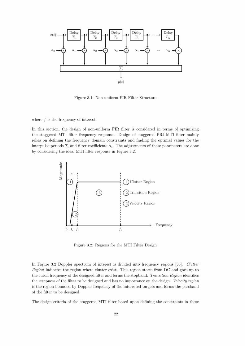
Figure 3.1 Non-uniform FIR Filter Structure . . . . . . . . . . . . . . . . . . . . . . . . 22

Figure 3.2 Regions for the MTI Filter Design . . . . . . . . . . . . . . . . . . . . . . . . 22

Figure 3.3 Performance Measures of the Staggered PRF MTI Filter Design . . . . . . . 24

Figure 3.4 Frequency Response of Desired Highpass Filter . . . . . . . . . . . . . . . . 25

Figure 3.5 Frequency Response of Least Square Design with Different W Values . . . . 29

Figure 3.6 Effect of W on MSA, SA, MPE and MD for Least Square Design . . . . . . 30

Figure 3.7 Frequency Response of Convex Design with Different W Values . . . . . . . 33

Figure 3.8 Effect of W on MSA, SA, MPE and MD for Convex Design . . . . . . . . . 34

Figure 3.9 Frequency Response of Min-Max Design with Different W Values . . . . . . 37

Figure 3.10 Effect ofW on MSA, SA, MPE and MD for Min-max Design for Same InitialCoefficients . . . . . . . . . . . . . . . . . . . . . . . . . . . . . . . . . . . . . . . . 38

Figure 3.11 Frequency Response of Min-Max Design for Different Initial Conditions withthe Same W Values . . . . . . . . . . . . . . . . . . . . . . . . . . . . . . . . . . . . 40

Figure 3.12 Effect of Initial Filter Coefficients on Performance Measures of Min-MaxDesign for Same W Values . . . . . . . . . . . . . . . . . . . . . . . . . . . . . . . . 41

Figure 3.13 Min-Max Design for Different Stopband Attenuation Requirement with Dif-ferent Initial Conditions and W Values . . . . . . . . . . . . . . . . . . . . . . . . . 42

Figure 3.14 Comparison of Designed Filters with Binomial and Prinsen’s Filter withSame Stopband Attenuation Requirement . . . . . . . . . . . . . . . . . . . . . . . 46

xv

Figure 3.15 Comparison of Designed Filters with Binomial and Prinsen’s Filter withSmaller Cutoff Frequency . . . . . . . . . . . . . . . . . . . . . . . . . . . . . . . . . 47

Figure 3.16 Comparison of Designed Filters with Binomial and Prinsen’s Filter withBigger Cutoff Frequency . . . . . . . . . . . . . . . . . . . . . . . . . . . . . . . . . 48

Figure 3.17 Comparison of Designed Filters with Binomial and Prinsen Filter’s withLarger Velocity Band . . . . . . . . . . . . . . . . . . . . . . . . . . . . . . . . . . . 49

Figure 4.1 Gaussian Clutter Power Spectrum Density Model . . . . . . . . . . . . . . . 52

Figure 4.2 Comparison of Optimum MTI Filters with Different Clutter PSD’s . . . . . 53

Figure 4.3 Frequency Response Comparison of Designed Filters with Prinsen’s Filter . 56

Figure 4.4 Improvement Factor Comparison of Designed Filters with Prinsen’s Filterwith Gaussian Clutter PSD . . . . . . . . . . . . . . . . . . . . . . . . . . . . . . . 57

Figure 4.5 Improvement Factor Comparison of Designed Filters with Prinsen’s Filterwith Gaussian Clutter PSD with Larger Doppler Spread . . . . . . . . . . . . . . . 58

Figure 4.6 Frequency Response Comparison of Minmax-IF Filter with Other FilterDesigns . . . . . . . . . . . . . . . . . . . . . . . . . . . . . . . . . . . . . . . . . . . 61

Figure 4.7 Improvement Factor Comparison of Designed Filters with Gaussian Clutter 62

Figure 4.8 Improvement Factor Comparison of Designed Filters with Gaussian Clutterwith Larger Doppler Spread . . . . . . . . . . . . . . . . . . . . . . . . . . . . . . . 63

Figure 4.9 Processing of Received Pulses with Multiple Filter Structure with TimeVarying Coefficients . . . . . . . . . . . . . . . . . . . . . . . . . . . . . . . . . . . . 65

Figure 4.10 Frequency Response of Designed Filters for Stagger Ratio 16:20:17:22 (SingleFilter) . . . . . . . . . . . . . . . . . . . . . . . . . . . . . . . . . . . . . . . . . . . 68

Figure 4.11 Improvement Factor Plots of Designed Filters for Stagger Ratio 16:20:17:22(Single Filter) . . . . . . . . . . . . . . . . . . . . . . . . . . . . . . . . . . . . . . . 69

Figure 4.12 Total Power Response of Designed Time Invariant Single Filters for StaggerRatio 16:20:17:22:16:20:17 (Multiple Filter) . . . . . . . . . . . . . . . . . . . . . . . 70

Figure 4.13 Improvement Factor Plots of Designed Time Invariant Single Filters forStagger Ratio 16:20:17:22:16:20:17 (Multiple Filter) . . . . . . . . . . . . . . . . . . 71

Figure 4.14 Passband Response of Designed Single Filters for Stagger Ratios 16:20:17:22,20:17:22:16, 17:22:16:20, 22:16:20:17 . . . . . . . . . . . . . . . . . . . . . . . . . . . 72

Figure 4.15 Stopband Response of Designed Single Filters for Stagger Ratios 16:20:17:22,20:17:22:16, 17:22:16:20, 22:16:20:17 . . . . . . . . . . . . . . . . . . . . . . . . . . . 73

Figure 4.16 Passband Response of Designed Filters for Stagger Ratios 16:20:17:22, 20:17:22:16,17:22:16:20, 22:16:20:17 . . . . . . . . . . . . . . . . . . . . . . . . . . . . . . . . . . 75

Figure 4.17 Stopband Response of Designed Filters for Stagger Ratios 16:20:17:22, 20:17:22:16,17:22:16:20, 22:16:20:17 . . . . . . . . . . . . . . . . . . . . . . . . . . . . . . . . . . 76

Figure 4.18 Total Power Response of Designed Multiple Filters used for Stagger Ratio16:20:17:22:16:20:17 (Multiple Filter) . . . . . . . . . . . . . . . . . . . . . . . . . . 78

Figure 4.19 Improvement Factor Plots of Designed Multiple Filters used for StaggerRatio 16:20:17:22:16:20:17 . . . . . . . . . . . . . . . . . . . . . . . . . . . . . . . . 79

Figure 5.1 Magnitude Response Comparison of Designed Filters with Hsiao’s Filter . . 83

Figure 5.2 Improvement Factor Plots of Designed Filters with Hsiao’s Filter . . . . . . 84

xvi

Figure 5.3 Magnitude Response Comparison of Designed Filters with Jacomini’s Filter 86

Figure 5.4 Improvement Factor Plots of Designed Filters with Jacomini’s Filter . . . . 87

Figure 5.5 Magnitude Response Comparison of Designed Filters with Ewell’s Filter . . 89

Figure 5.6 Improvement Factor Plots of Designed Filters with Ewell’s Filter . . . . . . 90

Figure 5.7 Magnitude Response Comparison of Designed Filters with Zuyin’s Filter . . 92

Figure 5.8 Improvement Factor Plots of Designed Filters with Zuyin’s Filter . . . . . . 93

xvii

CHAPTER 1

INTRODUCTION

Detection of moving targets in strong clutter has been one of the most important tasks of theradar systems throughout the history. Through the evolution of radar systems a number oftechniques and methods are developed in order to increase the target detection capability ofthe radar systems in strong clutter. One of the basic methods is the usage of Moving TargetIndication (MTI) signal processor. As the name implies, it is used to indicate the presence ofmoving targets in heavy clutter by discriminating the component of the return echo due tomoving targets from stationary background.

First MTI designs were based on the analog delay line cancellers, which are used for cancellingstationary clutter by subtracting the successive returns in order to improve the detection ofthe target component. With the introduction of digital systems, digital filters are developedand improvements in performance have been attained.

Design of the MTI processor is mainly based on the design of filter structure for clutter attenu-ation. For stationary clutter attenuation, simple highpass filters provide sufficient attenuation,whereas higher order filters can be required to sufficiently attenuate clutter with significantDoppler spread.

Digital implementation of the MTI signal processor filter has a periodic characteristic due touniform sampling with constant pulse repetition frequency (PRF). Because of the periodicnature, the moving targets having Doppler frequencies which are integer multiples of PRFare cancelled by the MTI filter along with the background clutter. Therefore, these movingtargets are not seen by the radar. Velocities that correspond to the undetected frequencies arecalled blind speeds [4]. There are different approaches for the solution of this problem in theliterature. One of them is staggering the interpulse durations, that is the usage of differentinterpulse periods instead of a single one [5].

The usage of staggered interpulse durations improves the blind speed performance in MTIradars. It should be noted that the improvement in blind speed comes at almost no additionalcomputational cost. An important disadvantage of non-uniform sampling is the passband rip-ples which are much larger in comparison to uniform PRI systems. Due to these ripples, thefluctuations of signal power at the MTI filter output may degrade the detection performancefor particular Doppler frequencies. Therefore, it is important to design MTI filters by consid-ering the detection probability and performance of the radar system for the specific Dopplerfrequencies.

Design of staggered MTI filters depends upon the radar system parameters that are related

1

to the detection probability and clutter attenuation. Based upon these parameters, staggeredMTI filter design comprises on the optimization of two sets of parameters: the interpulsetime durations and the filter coefficients. The unambiguous range and velocity specificationsimpose constraints on the interpulse periods. The desired clutter attenuation affects the valuesof filter coefficients [6].

Our goal in this thesis is to apply classical uniform filter design techniques and present flexiblesolution to the non-uniform MTI filter design for a given set of interpulse durations. Designedfilters can be adopted to different scenarios having different clutter attenuation and Dopplerfrequency band of interest specifications. The presented designs provide the opportunity forthe selection of the best interpulse periods from a set of suitable candidates by satisfying theunambiguous range-velocity constraints.

In the present work, we study three widely adopted FIR filter design techniques, the leastsquare, convex and min-max filter design. The systematic design of each approach is described.A number of performance measures are defined and comparison between different filters isgiven for the various scenarios. Obtained results indicate that it is possible to design non-uniform filters according to different cutoff frequencies and clutter attenuation values. One canoptimize the filter response by defining the clutter attenuation, cutoff frequency and interestedDoppler frequency band and selecting a suitable weight factor.

A possible novelty of the present work is the design of a min-max MTI filter based upon im-provement factor of the optimum filter. This design technique is different from the previouslystated min-max filter design and uses the information of improvement factor of optimum filterresponse for a specified clutter power spectrum density.

Throughout the thesis work, a literature survey related to design of staggered MTI filtersis given and a detailed description of the mentioned filter design approaches are presentedwith specific algorithm steps and performance comparisons for several parameters. Availabledesigns in the literature are implemented and numerical comparisons with these are given.

The organization of thesis is as follows: In Chapter 2, the background information relatedto MTI filter is given. Different configurations of the MTI filters are given along with theirfrequency response characteristics. The blind speed problem is explained and the staggeredPRF MTI filter solution is given.

In Chapter 3, the design of three different types of non-recursive staggered PRF MTI filtersare given. First, the properties and design constraints of the non-uniform FIR filter designare explained. Later, three types of design approaches are presented in relation with the non-uniform FIR filter design. Finally a numerical comparison between previously designed filtersare made.

In Chapter 4, the clutter attenuation is taken into account for the designed filters. First,the definition and the properties of clutter are presented. The effect of clutter on the earlierdesigns are discussed and the results are compared with respect to a number of figures of merits.Later, a novel min-max filter design approach is explained based upon the improvement factorof optimum filter. Finally, the multiple filter approach is described with time varying filtercoefficients.

In Chapter 5, the simulation results of the designed filters with the designs in the literature aregiven. For each design in the literature, the design approach is explained with examples and

2

comparisons of the designed filters with respect to performance measures and improvementfactor are given.

In Chapter 6, concluding remarks are presented, obtained results are summarized and therelated future work is described.

3

CHAPTER 2

BACKGROUND

2.1 Moving Target Indication (MTI) Radar

It is difficult to distinguish a moving target in the presence of ground-clutter or sea-clutterenvironment due to strong clutter echos. Detection of moving targets in these conditions isperformed using Moving Target Indication (MTI) radar. The MTI radar is a type of pulseradar that uses the non-zero Doppler shift of moving targets for their detection [5] by cancellingthe stationary background clutter.

There are different types of MTI Radars classified according to operation modes, environmentsand used signal processing algorithms. Coherent MTI Radar is the type in which a movingtarget is detected as a result of pulse-to-pulse change in echo phase relative to the phase of acoherent reference oscillator [7]. In other words, it is a system that uses the phase differenceresulting from Doppler effect to separate the moving targets from stationary backgroundclutter. Pulses are transmitted and received echos are compared with the signal producedby the coherent reference oscillator. Due to Doppler shift, moving target component of thereceived echo has a phase difference in comparison to the reference oscillator signal and canbe discriminated from clutter.

Another type of MTI radar that uses the clutter echo as the reference signal to discriminatethe Doppler-shifted information of target echo is known as Non-Coherent MTI or externallyCoherent MTI [5]. This type of MTI is simpler than coherent MTI; but it requires the presenceof clutter for detecting the moving targets. Due to clutter dependence, Non-Coherent MTIimplemented as a mode and can be switched on or off depending on the presence or absenceof strong clutter reference. [5].

MTI Radars used in airborne applications named as Airborne MTI or AMTI. Operationprinciple of this type is similar to the Coherent MTI ; however, compensation for the movingradar platform is necessary. The Doppler shift of the received echos change depending on therelative motion of the moving radar platform and target. After the compensation of relativemotion between platforms, moving targets can be detected by suppressing the stationaryclutter.

Adaptive MTI Radar is another type of MTI radar that adapts itself to the clutter. Accordingto change in clutter characteristics, the coefficients of the MTI filter are changed on timebasis. Adaptation to the clutter can be achieved by different estimation techniques for cluttercovariance matrix [8].

5

Different from other MTI techniques, Area MTI radar does not use Doppler shift directly andcompares the envelope-detected outputs of successive scans to detect the targets that move inrange or azimuth between scans [5].

2.1.1 Operation of a Coherent MTI Radar

The operation of a Coherent MTI Radar is based upon discrimination of the radar return bycomparing the phases of all echoes with reference (coherent) phase. Simplified structure of aCoherent MTI Radar is illustrated in Figure 2.1.

ii

DelayT

∑

−

+

MTI FILTER

×

PHASE DETECTOR

RF OSCILLATOR

Bipolar Video

TRANSMITTERDUPLEXER

ANTENNA

MOVING TARGET

Figure 2.1: Simplified Block Diagram of A Coherent MTI System [2]

Here RF oscillator is used in the transmitter and also as reference for the received echos forphase comparison [2]. Duplexer is used for switching between transmission and receptionoperations. A radar return usually contains two components; target component and cluttercomponent [9]. Clutter component signal arises due to stationary background objects and hasmuch stronger than the target component signal, in general. Discrimination of the target andclutter components made by comparing successive received echos in terms of phase propertiesand filtering the stationary background clutter. The phase change due to target motion resultsin a component changing from pulse to pulse, whereas the clutter component stays the same.This provides a way to discriminate the clutter and target components by evaluating the phasesof successive return echos. Phase comparison is implemented by delaying the previous echo

6

and subtracting from the current one. In frequency domain, the operation of the MTI filtercorresponds to the attenuation of frequencies associated with the clutter spectrum withouta significant (hopefully) reduction of the Doppler frequencies of moving targets. This showsthat MTI filter is a highpass filter.

Figure 2.2 shows the operation of MTI. An examination of Figure 2.2 reveals that the magni-tude response of the received echos stays same from pulse to pulse mostly. By looking at thesuccessively received returns, it is not easy to extract the moving targets components fromclutter component. However it is seen that, by subtracting the successive returns with MTIfilter, the moving target component can be easily differentiated from the clutter. This resultcan be seen from the last sub plot given in Figure 2.2.

7

2 2.5 3 3.5 4 4.5 5 5.5 60

20

40

60

80Total Return Echo for Pulse 1 and Pulse 2

Distance (km)

Amplitud

e(dB)

P1P2

2 2.5 3 3.5 4 4.5 5 5.5 60

20

40

60


Distance (km)

Amplitud

e(dB)

P3P4

2 2.5 3 3.5 4 4.5 5 5.5 60

20

40

60


Distance (km)

Amplitud

e(dB)

P5P6

2 2.5 3 3.5 4 4.5 5 5.5 60

20

40

60

80↓Moving Target-1 ↓Moving Target-2

Total Return After MTI Filter

Distance (km)

Amplitud

e(dB)

P2-P1P3-P2P4-P3P5-P4P6-P5

Figure 2.2: MTI Processing of Received Echos from Successive Transmitted Pulses

2.2 MTI Filtering

Different types of MTI filters are developed and have been used through the radar history.These filters are designed according to hardware specifications and the operation constraintsof the radar system. A typical MTI filter has a highpass filter characteristics that is designed

8

for rejecting zero or small Doppler frequencies and passing higher frequencies correspondingto the moving targets. MTI filters can be classified in three main categories as follows.

2.2.1 Delay Line Cancellers

The delay line canceller is an analog technique used in the first MTI signal processor design.The operation is based on subtracting two consecutive radar returns. The structure of singledelay line canceller can be given in Figure 2.3.

x(t) ii y(t)

DelayT

∑

−

+

Figure 2.3: Filter Structure of the Single Delay Line Canceller

Time domain difference equation of the single delay line canceller with pulse repetition interval(PRI) T is given in (2.1)

y(t) = x(t)− x(t− T ) (2.1)

The frequency response characteristics of the single delay line canceller can be written bytaking the Fourier Transform (F) of the time domain difference equation as in (2.2)

F{y(t)} = F{x(t)− x(t− T )}Y (f) = X(f)(1− e−j2πfT )

Hsdlc(f) =Y (f)

X(f)= e−j2πfT/2(ej2πfT/2 − e−j2πfT/2)

= 2j sin(2πfT/2)e−j2πfT/2

= 2j sin(πfT )e−jπfT (2.2)

The magnitude of the frequency response of the single delay line canceller with the pulserepetition interval of T is given in (2.3) and plotted in Figure 2.4.

|Hsdlc| = 2 sin (πfT ) (2.3)

Single delay line canceller rejects the stationary clutter which has zero Doppler shift. Whenthe clutter has spread in the spectrum, then the performance of the single delay line cancellerdecreases and the clutter residue resides at the filter output, especially at small Dopplerfrequencies. When slow moving targets are present, then the detection performance of thesetargets are affected by the clutter residue. In other words, insufficient clutter attenuationdecreases the performance of the single delay line canceller. Due to this reason, the singledelay line canceller is not sufficient for the rejection of clutter with large spread in spectrum.

9

0 1/T 2/T 3/T 4/T 5/T 6/T0

0.5

1

1.5

2Magnitude Response

Frequency (Hz)

Magnitude

(V)

Figure 2.4: Magnitude Response of Single Delay Line Canceller

As a solution to this problem, the usage of cascaded single delay line cancellers are proposed.By cascading two single delay line cancellers the double delay line canceller is formed. Figure2.5 shows the filter structure of the double delay line canceller.

x(t) ii

DelayT

∑

−

+

DelayT

∑

−

+

y(t)ii

Figure 2.5: Filter Structure of the Double Delay Line Canceller

The magnitude response of the double delay line canceller can be calculated using the singledelay line canceller response as in (2.4) and pointed out in Figure 2.6 together with the singledelay line canceller magnitude response for the purpose of comparison.

|Hddlc(f)| = |Hsdlc(f)|2 = (2|sin(πfT )|)2 = 4 sin (πfT )2 (2.4)

As seen from Figure 2.6, the double delay line canceller performance is greater in terms of theattenuation of non-zero spread clutter spectrum. By increasing the number of cascaded singledelay line cancellers, an improved response in terms of attenuating finite width clutter can beobtained. Figure 2.7 indicates the response of cascaded single cancellers. The responses of thecascaded single cancellers can be calculated by taking the Nth power of the single delay linecanceller response as in (2.5). Here N represents the number of single delay line cancellersthat are cascaded.

|HNdlc(f)| = (2|sin(πfT )|)N (2.5)

10

0 1/T 2/T 3/T 4/T 5/T 6/T0

1

2

3

4

Frequency (Hz)

Magnitude

(V)

Magnitude Response

Single CancellerDouble Canceller

Figure 2.6: Magnitude Response Comparison of Single and Double Delay Line Cancellers

0 0.05 0.1 0.15 0.2 0.25 0.3 0.35 0.4 0.45 0.50

1

2

3

4

Normalized Frequency

Magnitude

(V)

Magnitude Response

N=1N=2N=3N=4N=5

Figure 2.7: Magnitude Response Comparison of Cascaded Single Delay Line Cancellers

2.2.2 FIR Type MTI Filters

Finite-Impulse-Response (FIR) filters can be used for MTI processing if the filter weights arechosen in order to obtain a highpass filter characteristics. General structure of the FIR filtersfor uniform pulse repetition interval are given in Figure 2.8.

One of the simplest and widely used uniform FIR type MTI filter is the Binomial MTI filterwhose coefficients are formed by binomial numbers. This method corresponds to the cascadeof single delay line cancellers. As an example, the double delay line canceller can be arrangedas FIR type in Figure 2.9.

These cascade arrangements of the single delay line cancellers as transversal filter structure is

11

x(t)DelayT

DelayT

DelayT

DelayT

... DelayT

w0 × w1 × w2 × w3 × ...w4 × wN ×

∑

y(t)

Figure 2.8: General Structure of a Uniform FIR Filter

called as N-pulse cancellers since N pulse is processed for N − 1 cascaded single cancellers.For example, a double delay line canceller named as 3-pulse canceller can be represented asan FIR filter as in Figure 2.9.

x(t)DelayT

DelayT

1 × −2 × 1 ×

∑

y(t)

Figure 2.9: Double Delay Line Canceller Representation as a Transversal Filter Structure

For cascaded single delay line cancellers, z-transform of the time domain difference equationcan be written as

HNdlc(z) = (1− z−1)N (2.6)

If the equation (2.6) is expanded, the coefficients are the binomial numbers with alternatingsigns. Corresponding filter weights of the N-pulse cancellers can be calculated using thefollowing equation:

wi = (−1)i−1N !

(N − i+ 1)!(i− 1)!, i = 1, 2, . . . , N + 1 (2.7)

For the first 5-pulse canceller structures, filter weights are given in Table 2.1. Usage of thebinomial coefficients lead to naming of N-pulse Cancellers asMTI Filter with Binomial Weightsin the literature.

12

Table 2.1: Filter Weights for First 5 N-pulse Cancellers

N-pulse Canceller Filter Weights

2-pulse [1,-1]

3-pulse [1,-2,1]

4-pulse [1,-3,3,-1]

5-pulse [1,-4,6,-4,1]

Besides Binomial MTI filter, different techniques and designs are proposed in the literaturefor adjusting the coefficients of the FIR type MTI filters [10], [6], [11]. Most of the studies seekthe optimum MTI filter for clutter rejection and propose different optimization techniques likequadratic programming for calculating the filter weights [10]. The constraints of these designsare based on minimization of output clutter and attenuation of stationary clutter.

2.2.3 Recursive MTI Filters

Recursive filters are also used as an MTI signal processor. They are utilized to shape thestopband response. Recursive filters have the feedback coefficients and feedforward coefficients.An example direct-form structure is given in Figure 2.10. Using recursive filters, stopbandof the filter can be shaped more easily due to additional degrees of freedom that comes fromfeedback coefficients. However, these filters have poor transient response. This type of filterscan be designed using classical z-transform theory and pole-zero analysis [3], [12]. Z-domaintransfer function of a recursive filter is given in (2.8). As an example, magnitude responses ofthree different shaped MTI filters are given in Figure 2.11.

H(z) =β0 + β1z

−1 + β2z−2 + . . .+ βMz

−M

1 + α1z−1 + α2z−1 + . . .+ αNz−N(2.8)

After the examination of three types of MTI filters, we present the design criteria for the MTIfilters. There are different figures of merit for the performance comparison of the MTI filters.These are stated as MTI Improvement Factor, subclutter visibility, MTI gain, MTI response,clutter attenuation, clutter visibility factor and cancellation ratio in [4]. The most commonlyused and accepted measure is the MTI Improvement factor whose definition includes the effectof clutter attenuation and MTI gain.

2.3 MTI Improvement Factor

MTI Improvement Factor is a performance measure for the clutter attenuation. It is definedas “the signal-to-clutter power ratio at the output of the MTI filter to the signal-to-clutterpower ratio at the input, averaged uniformly over all target velocities of interest.” [7]. It canbe expressed as

13

x(t)DelayT

DelayT

DelayT

DelayT

... DelayT

∑

∑

β0 × β1 ×

−α1×

β2 ×

−α2×

β3 ×

−α3×

β4 ×

−α4×

... βM ×

−αN×

∑

y(t)

Figure 2.10: IIR Filter Structure

0 100 200 300 400 500 6000

0.2

0.4

0.6

0.8

1

1.2Magnitude Response

Frequency - Hz

Normalized

Magnitude

ButterworthTriple BinomialChebyshev

Figure 2.11: Magnitude Response of Different Types of Shaped MTI Filters [3]

Improvement Factor = IF =(SCR)out(SCR)in

(2.9)

where SCRout and SCRin represent average signal-to-clutter ratio at the output and input ofthe MTI filter respectively. Improvement factor can be thought of average SCR improvementof the MTI filter, not at a particular frequency. The improvement factor can be furtherdescribed as follows. If the received signal is

14

r = s(θ) + c (2.10)

where r, s(θ) and c are N × 1 column vectors that represent the received signal, cluttercomponent and signal component of the received echo respectively. θ is phase change in PRIseconds corresponding to Doppler effect. Average power at the input can be written as theaddition of signal and clutter power if the signal and clutter are assumed to be zero mean anduncorrelated. It is given by

Pi = E{||s(θ) + c||2}= E{s(θ)Hs(θ)}+ E{cHc} (2.11)

where the first and second terms represent signal and clutter powers at the input respectively.

After filtering the input signal with an FIR MTI filter with N × 1 coefficient vector α, powerof the filtered signal can be written as follows:

Po = E{||αH [s(θ) + c]||2}= E{αHs(θ)sH(θ)α}+ E{αHccHα} (2.12)

Similar to the input power case, the first and second terms represent the signal and clutterpowers at the output of the MTI filter respectively.

Using (2.11) and (2.12), SCRin and SCRout can be written as follows

SCRout =E{αHs(θ)sH(θ)α}

E{αHccHα} (2.13)

SCRin =E{s(θ)Hs(θ)}

E{cHc} (2.14)

By putting SCR equations in (2.9), improvement factor can be rewritten as in (2.15)

IF (θ) =E{αHs(θ)sH(θ)α}

E{s(θ)Hs(θ)}× E{cHc}

E{αHccHα}

=αHRsα

αHRcα(2.15)

where Rc and Rs are normalized clutter and signal covariance matrices respectively.

By using the obtained improvement factor equation, MTI improvement factor for the coherentMTI case with FIR type filter can be expressed as in (2.16) by assuming uniform distribution

15

for Doppler frequencies of the signal.

IF =

∫ 2π

0

IF (θ)dθ =

N−1∑

j=0

α2j

N−1∑

j=0

N−1∑

k=0

αjαkρ(j, k)

(2.16)

where αj , αk’s are the MTI’s real weights, ρ(j, k) is the correlation coefficient of clutter returnsbetween the j’th and k’th pulses. and N is the number of pulses processed by the MTI.

As seen from the improvement factor relation, the improvement factor depends upon filtercoefficients and clutter covariance matrix. Hsiao [13] shows that optimal MTI filter dependsupon clutter covariance matrix and weights of the optimal MTI are given by the elements ofthe eigenvector that corresponds to the minimum eigenvalue of the clutter covariance matrix.

2.4 Blind Speed Problem

One of the main disadvantages of the usage of uniform interpulse duration in digital MTIfilters is that moving targets with Doppler frequencies that are integer multiples of the PRFwill be cancelled together with clutter because of periodic sampling of Doppler frequency. Thenulls that result from the periodic sampling characteristics of the system are given by:

fd =n

PRI= n× PRF (2.17)

The speeds correspond to these undetected Doppler frequencies are named as blind speeds ([9])and can be calculated as in (2.18) .

Vblind = n× λ/2× PRF =n× c× PRF

2f(2.18)

where λ is wavelength and PRF is pulse repetition frequency and f is the operating frequency.As an example, an X-Band radar that has 500 µs uniform PRI exhibits blind speeds at300 m/s, 600 m/s, 900 m/s, . . . .

Table 2.2 illustrates widely used frequency bands. For high frequency bands, first blind speedscan have smaller values, typically not sufficient to detect possible targets of interest for thesebands. Therefore it is essential to increase the value of first blind speed for the designatedradar frequency bands.

Considering the blind speed equation (2.18), four methods are proposed in order to increasethe first blind speed of a radar system [5]. These methods can be stated as

• Usage of lower center frequencies for operation frequency of radar system

• Increasing the pulse repetition frequency

• Usage of multiple pulse repetition intervals

16

Table 2.2: First Blind Speeds for Different Radar Bands [1]

PRF (Hz) 10000 1000 250

Maximum Range (km) 15.00 150.00 600.00

Band

Frequency US UK ECM First Blind Speeds (m/s)

600 MHz UHF UHF C 2500.00 250.00 62.5

1300 MHz L L D 1153.85 115.38 28.85

3000 MHz S S E..F 500.00 50.00 12.50

5500 MHz C C G 272.73 27.27 6.82

10000 MHz X X I 150.00 15.00 3.75

16000 MHz Ku J J 93.75 9.38 2.34

30000 MHz Ka Q K 50.00 5.00 1.25

• Usage of multiple frequencies for operation frequency of radar system

Suggested solutions can be used together or individually. However each one of the solutionshave some negative effects on the operation of the radar system.

Operation with a lower center frequencies results in a decrease in range and angle resolutionsof the radar. Lower frequency band is used in civil applications. Therefore, lowering thefrequency is not a desirable choice for many of radar systems. Increasing the pulse repetitionfrequency decreases the unambiguous range and causes range ambiguities. Usage of more thanone PRF’s increases first blind speed of the radar system whereas multiple-time-around clutterechoes will fold into different ranges. Operating the radar at more than one frequency causesstress on transmitter and is not desirable within the usual frequency bands allocated [5].

Widely used solution to blind speed problem in MTI filters is the usage of non-uniform (stag-gered) PRI [9]. With this method the first blind speed is increased with respect to a uniformPRI MTI system. Two main staggering approaches utilized generally: pulse to pulse and blockto block staggering. Pulse to pulse staggering is performed by changing the interpulse periodfrom pulse to pulse. This method is suitable for MTI processing and resistant to electronicjamming. On the other hand, block-to-block staggering is utilized by changing the interpulseperiod after transmitting a group of pulses with same PRI and used widely in pulse-Dopplerradars.

2.5 Staggered PRI Design

Staggered PRI design is based upon defining the interpulse durations according to range andvelocity specifications of the radar system. IfN interpulse durations denoted as T1, T2, T3, . . . TNis taken into account, the period of the stagger pattern is given by

Tp =

N∑

i=1

Ti (2.19)

17

Each interpulse duration can be expressed as multiple of greatest common factor of the set ofinterpulse durations.

Ti = kiTgcd (2.20)

Here ki’s are integers that define the stagger ratio of the corresponding interpulse durationsand Tgcd is the greatest common divisor of the time durations set.

The coefficient ki define the improvement of the first blind speed of the staggered systemwhich is given by average interpulse duration

Tav =1

N

N∑

i=1

kiTgcd (2.21)

As an example, for a 2-PRI system with T1 = 3T and T2 = 5T , the frequency response of thestaggered system with T1 and T2 is compared with non-staggered system with uniform PRIof 4T is shown in Figure 2.12.

0 1 2 3 4 5 6 7 8−80

−60

−40

−20

0

20Magnitude Response for Uniform and Staggered PRI

Normalized Frequency (f / fbs)

Magnitude

(dB)

UniformNon-Uniform

Figure 2.12: Magnitude Response Comparison of MTI Filter with Uniform and Staggered PRI

As it is seen from Figure 2.12, by using two different PRI values, first blind speed of thestaggered system increased 4 times with respect to non-staggered system with PRI of 4T .

Usage of PRI staggering improves blind speed, but because of the non-uniform sampling thefrequency response fluctuates in the passband which results in degradation in the improvementfactor. It is important to provide a flat passband response for an equally probable targetdetection over the velocity band of interest. In addition, adjustment of interpulse durations isimportant in terms of minimum unambiguous range and dwell time. Therefore, it is necessaryto optimize the stagger periods according to the other specifications.

Different stagger patterns are given in the literature. One of the simplest techniques is addinginteger values to the desired multiple of the first blind speed [2]. For example, for a four andfive-period stagger schemes -3,2,-1,3 and -6,5,-4,4,1 integer groups are used respectively. If a

18

14 times and 57 times blind speed increase is desired, the corresponding stagger ratios will be11 : 16 : 13 : 17 and 51 : 62 : 53 : 61 : 58.

It is also discussed to use stagger periods according to analytical patterns. Interpulse durationscan be changed according to linear, sinusoidal, symmetric, wobulated and random manner[14], [15]. Small deviations from the average interpulse period are also implemented [16].As a different approach, choosing the stagger intervals according to frequency response ofnon-uniform transversal filter is discussed in [17].

Other solutions for stagger optimization pursue analytical methods through of searching andobtaining the best possible stagger scheme with respect to different constraints [18], [19], [20],[21], [22]. To this aim, an algorithmic solution can be described as follows.

• Define a cost function

• Define an initial stagger scheme

• Calculate cost function

• Change stagger intervals

• Recalculate the cost function

• If the cost function improved, choose new stagger values

Along with the stagger interval adjustment, coefficients of the MTI filter that process staggeredpulses must be optimized in terms of satisfactory clutter attenuation and system performance.The goal of the MTI filter design is to provide maximum amount of clutter suppression concur-rently with the least amount desired signal suppression (flat passband). Design of staggeredMTI filter can be implemented in terms of two general cases. After the selection of theinterpulse durations according to range-velocity constraints, coefficients of the non-uniformfilter can be selected to satisfy the required clutter attenuation and improvement factor asstudied in [11], [18], [6], [23], [24]. Alternatively, optimization of the stagger intervals and fil-ter coefficients are carried out together by considering range-velocity and clutter attenuationconstraints [19], [25], [20].

19

CHAPTER 3

NON-UNIFORM MTI FILTER DESIGN

In this chapter staggered MTI filter designs are studied from the perspective of filter designwith non-uniform samples. First, properties and constraints of the non-uniform FIR filterdesign is presented. Second, designed filters for non-uniform MTI processing explained indetail with defined performance measures. Finally, a comparison of designed filters with theselected designs is given in terms of the performance measures.

3.1 Non-uniform FIR Filter Design

Non-uniform sampling and filtering have been frequently used in several applications in theprocessing of acoustic, image and radio frequency signals [26], [27], [28], [29], [30], [31], [32],[33], [34]. The studies mostly focus on decreasing the total sampling time, reconstructionof the non-uniformly sampled signals, and improving the system performance. Most of thestudies focus on FIR type implementations ([29], [27], [28], [31], [32]), but IIR type designsare also considered ([30], [35]).

The general filter structure of the discrete non-uniform FIR type filter is illustrated in Fig-ure 3.1. The output signal is obtained by summation of the linear combination of the non-uniformly sampled input signal. The impulse response of this transversal filter is expressed bythe following relation

h(t) =

N−1∑

n=0

αnδ(t− tn) (3.1)

where αn are the filter coefficients and tn are the sampling times given by

tn =

n−1∑

i=0

Ti, n ≥ 1

0, n = 0

(3.2)

where Ti’s are the interpulse periods.

The corresponding frequency response of the filter is given by

H(f) =

N−1∑

i=0

αie−j2πfti (3.3)

21

x(t)DelayT1

DelayT2

DelayT3

DelayT4

... DelayTN

α0 × α1 × α2 × α3 × ...α4 × αN ×

∑

y(t)

Figure 3.1: Non-uniform FIR Filter Structure

where f is the frequency of interest.

In this section, the design of non-uniform FIR filter is considered in terms of optimizingthe staggered MTI filter frequency response. Design of staggered PRI MTI filter mainlyrelies on defining the frequency domain constraints and finding the optimal values for theinterpulse periods Ti and filter coefficients αi. The adjustments of these parameters are doneby considering the ideal MTI filter response in Figure 3.2.

1

2

3

1

2

3

Clutter Region

Transition Region

Velocity Region

Magnitude

Frequency0 fc ft fp

Figure 3.2: Regions for the MTI Filter Design

In Figure 3.2 Doppler spectrum of interest is divided into frequency regions [36]. ClutterRegion indicates the region where clutter exist. This region starts from DC and goes up tothe cutoff frequency of the designed filter and forms the stopband. Transition Region identifiesthe steepness of the filter to be designed and has no importance on the design. Velocity regionis the region bounded by Doppler frequency of the interested targets and forms the passbandof the filter to be designed.

The design criteria of the staggered MTI filter based upon defining the constraints in these

22

regions and there is often a compromise between these performance metrics [5]. Possibleobjectives of the MTI filter design can be listed as follows;

• All targets in the velocity interval of interest be equally detectable

• Clutter at the output of the filter be minimum

• Required MTI improvement factor for the clutter attenuation be satisfied

• The deepest null in the passband should not be excessive

• Passband ripple should be minimized and kept uniform

The described objectives above form the design constraints for the staggered MTI filter. Inessence, the given objectives of the MTI filter can be condensed to

• Minimizing the passband ripple in velocity region

• Maximizing stopband attenuation in clutter region

It should be clear that both objectives can not be achieved simultaneously and a practicalsolution has to operate at a trade-off between these objectives. In order to obtain a flexiblesolution to these objectives; least square, convex and min-max filter design approaches arestudied. Before the examination of these filter design methods, we would like to present anumber of criterion that would be useful in the performance comparison of different designs.

3.2 Performance Measures of Staggered MTI Filter

Based on the stated constraints the design performance of the staggered MTI filter can becompared using the following criterion:

Mean Stopband Attenuation (MSA): This criteria indicates the clutter attenuation per-formance in clutter region. As the name implies it is the average of the SCR in the stopbandregion which is bounded by cutoff frequency fc. It is given by

MSA =1

fc

∫ fc

0

|H(f)|2df (3.4)

Stopband Attenuation @fc (SA): This is the value of filter magnitude response at thecutoff frequency fc. Since the frequency values smaller than fc (0 ≤ f ≤ fc) are typically at-tenuated more than the value at the cutoff frequency, this value can be considered to representthe worst case signal attenuation in the stopband. It is given by

SA = |H(fc)|2 (3.5)

Maximum Deviation (MD): This parameter indicates the maximum deviation from theideal flat response in the velocity region. This value is commonly seen at near transition regionand referred as the depth of the first null. It is given by

MD = max |Hd(f)−H(f)|2 (3.6)

23

Mean Passband Error (MPE): This criteria is to measure the flatness of the filter in thevelocity region. It is the average of the difference between ideal and designed filter responsesin the passband and given by the following equation

MPE =

∫ fp

ft

|Hd(f)−H(f)|2df (3.7)

whereHd(f) andH(f) are the frequency responses of the ideal and designed filters respectively.The limits of the integral are the lowest and highest frequency in the passband.

Schematic representation of the stated parameters is given in the Figure 3.3

Mean Passband Error

Maximum Deviation

Stopband Attenuation

Mean Stopband Attenuation

fdoppler/PRFmax

Magnitude(dB)

0 fc ft fp

Figure 3.3: Performance Measures of the Staggered PRF MTI Filter Design

It must be noted that in order to compare the frequency response of different filters a normal-ization is necessary for quantifying the rejection capabilities of the filters. Unity noise gainassumption is used for normalization of the responses and the filter weights are normalized asin (3.8) before the comparison of the filter responses.

αin =αi√√√√N−1∑

i=0

α2i

(3.8)

Doppler frequency interval is normalized by maximum pulse repetition frequency in order toconsider more general cases for specified stagger intervals, since maximum pulse repetitionfrequency determines the unambiguous range. Normalization with maximum pulse repetitionfrequency illustrates the increase with respect to minimum unambiguous range value and isconvenient for the performance comparison with the studies in the literature.

It is also important to note that maximum desired passband frequency fp must be smallerthan Fmax−fc for proper optimization that consider the periodicity of the frequency responseof the staggered MTI filter. Here Fmax represents the normalized first blind speed of MTIsystem with staggered PRI.

24

Based on the above criteria three main design approaches are studied in terms of optimizingthe filter coefficients for the given interpulse periods. First a least square (LS) approach isexamined, to obtain the filter coefficients that gives the near desired response in the sense ofminimum squared average error. Second, a convex optimization method (CVX) is studied.Later, a min-max (Min-max) approach design is implemented. The details of these filter designapproaches are explained in the following sections.

3.3 Least Square Design

The approach depends on minimizing the error between the desired filter and the designedfilter. The standard cost function for a least square sense designed filter is given by (3.9)

Jcost =

∫ fd

0

|Hd(f)−Hls(f)|2df (3.9)

where Hd(f) and Hls(f) indicates the frequency responses of the desired and least squaresense designed filter respectively.

Hd(f) is the ideal highpass filter whose frequency domain definition given by (3.10) and plottedin Figure 3.4

Hd(f) =

{0 if 0 ≤ f ≤ fc,1 if fc ≤ f ≤ fp,

(3.10)

Here fc is the cutoff frequency used for adjusting the notch of the filter according to attenuationbandwidth and fp is the bound for passband interval of Doppler frequency.

1

fdoppler/PRFmax

Magnitude

Hd(f)

0 fc ft fp

Figure 3.4: Frequency Response of Desired Highpass Filter

For non-uniform MTI filter, least square minimization problem can be stated as

minimize ||Hd(f)−Hls(f, αi)||

subject toN−1∑

i=0

αi = 0, x ∈ <

25

Here the∑N−1i=0 αi = 0 constraint used to suppress the DC value and ||.|| is the Euclidean

norm. It must be noted that with the inclusion of a linear constraint, least square design turnsinto a constraint least square design. By putting the equations in place, the cost function ofthe least square equation can be written as in (3.11). It must be noted that to simplify thepresentation only the positive frequency band is used.

Jcost(α, λ) =

∫ fd

0

|Hd(f)−N−1∑

i=0

αie−j2πfti |2df + λ

(N−1∑

i=0

αi

)(3.11)

The constraint equation is incorporated into the design via Lagrangian Multiplier λ. In orderto minimize this cost function it is required that

∂Jcost∂αi

= 0 (3.12)

By taking the partial derivatives of the cost function with respect to filter coefficients, we canget the following equation

∂Jcost∂αi

=

∫ fd

0

(Hd(f)−

N−1∑

n=0

αne−jπftn

)ej2πftidf +Nλ (3.13)

By equating, the partial derivatives given in (3.13) to zero for i = {0, 1, . . . , N}, we can getthe following linear equation system:

Aα = Hd + λ1 (3.14)

Here Hd is a N × 1 column vector with the k’th entry

Hd(k) =

∫ fd

fc

ej2πftkdf (3.15)

and A is a N ×N matrix with the i’th row and j’th column entry

A(i, j) =

∫ fd

0

e−j2πf(tj−ti)df (3.16)

1 is the N × 1 column vector with entries of 1

1 = [11 12 . . . 1N ]T (3.17)

Finally, the vector α in (3.14) is the vector of unknowns, that is the MTI filter coefficients.

In order to establish a trade-off between the objectives of clutter attenuation and passbandripple; we introduce a weight W to control the contribution of stopband error to the costfunction. The weight W changes the cost given in (3.18) as follows

JWcost =W∫ fc

0

|Hd(f)−Hls(f)|2df +

∫ fd

ft

|Hd(f)−Hls(f)|2df + λ(

N−1∑

i=0

αi) (3.18)

26

Optimization with the weighted cost function results in the following equation for the filtercoefficients

(W×Astop + Apass)α = Hd + λ1 (3.19)

In the last equation, we have

Astop(i, j) =

∫ fc

0


and

Apass(i, j) =

∫ fp

ft


It should be clear that by increasing W, the contribution of the stopband error to the costfunction is increased and therefore, the optimized filter provides more clutter suppression forhigher W values.

In order to find the least square MTI filter coefficients, Lagrangian Multiplier λ must bewritten in terms of other variables. By rewriting (3.19)

α = (W×Astop + Apass)−1(Hd + λ1) (3.22)

Since 1Tα = 0, Lagrangian Multiplier λ found as

1Tα = 1T(W×Astop + Apass)−1Hd + 1T(W×Astop + Apass)

−1λ1 = 0 (3.23)

λ =1T(W×Astop + Apass)

−1Hd

1T(W×Astop + Apass)−11(3.24)

As an example, frequency responses of least square design for different weight factors Wwith the specified stagger ratio of 25 : 30 : 27 : 31 (which is taken from [5]) is plotted inFigure 3.5. As it is seen from the figure, an increase in the weight factor W results in abigger attenuation in the clutter region and bigger mean square error in the velocity regionas expected. However the MD value does not depend upon weight factor linearly. This canbe seen from the performance criterion given for different weight factors in Table 3.1. ForW = 103, MD takes the value of 25.4 dB whereas it is 19.569 dB when W equals to 106.Since maximum deviation of the response is important in terms of detection performance, Wvalue must be selected according to minimum deviation after providing the required stopbandattenuation.

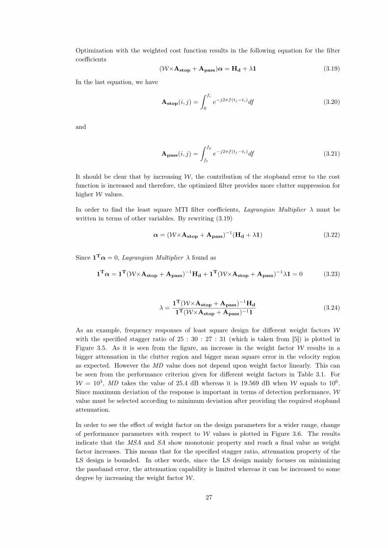
In order to see the effect of weight factor on the design parameters for a wider range, changeof performance parameters with respect to W values is plotted in Figure 3.6. The resultsindicate that the MSA and SA show monotonic property and reach a final value as weightfactor increases. This means that for the specified stagger ratio, attenuation property of theLS design is bounded. In other words, since the LS design mainly focuses on minimizingthe passband error, the attenuation capability is limited whereas it can be increased to somedegree by increasing the weight factor W.

27

Similarly,MPE reaches a final value asW increases, however it is not monotonously decreasing.Therefore, when smaller stopband attenuation is satisfactory for the system requirements,small W values can be selected for smaller average passband error.

As can be seen from the last sub figure in Figure 3.6, MD is the most sensitive criteria. AsW increases, MD fluctuates and poses a number of minimum values. For higher stopbandattenuation values, it reaches a constant value similar to other performance measures.

After evaluating the responses of the each performance measure, it is reasonable to choose Waccording to MD value.

28

0 2 4 6 8 10 12−80

−60

−40

−20

0

20LS Design, SR=25:30:27:31, fc = 0.04, ft = 0.1, fp = 10

fdoppler / PRFmax

|Hls

(f)|

(dB)

W = 103

W = 104

W = 105

W = 106

0 0.02 0.04 0.06 0.08 0.1 0.12−80

−60

−40

−20

0Zoomed Stopband Response

fdoppler / PRFmax

|Hls

(f)|

(dB)

W = 103

W = 104

W = 105

W = 106

Figure 3.5: Frequency Response of Least Square Design with Different W Values

Table 3.1: Performance Measures of Least Square Design for Different W Values

W MSA (dB) SA (dB) MPE (dB) MD (dB)

1000 -33.719 -24.884 -0.659 25.409

10000 -49.168 -40.470 -0.699 26.771

100000 -61.080 -46.445 -0.699 24.476

1e+06 -66.713 -50.030 -0.691 19.569

29

100 102 104 106 108 1010−100

−50

0MSA vs W , LS Design, SR=25:30:27:31, fc = 0.04, ft = 0.1, fp = 10

W

MSA

(dB)

100 102 104 106 108 1010−60

−40

−20

0SA vs W , LS Design, SR=25:30:27:31, fc = 0.04, ft = 0.1, fp = 10

W

SA(dB)

100 102 104 106 108 1010−1

−0.5

0MPE vs W , LS Design, SR=25:30:27:31, fc = 0.04, ft = 0.1, fp = 10

W

MPE

(dB)

100 102 104 106 108 10100

20

40

60MD vs W , LS Design, SR=25:30:27:31, fc = 0.04, ft = 0.1, fp = 10

W

MD

(dB)

Figure 3.6: Effect of W on MSA, SA, MPE and MD for Least Square Design

30

3.4 Convex Design

In convex filter design, staggered MTI filter design formulated as a convex optimization prob-lem. A convex optimization problem can be stated as [37]

minimize f0(x)

subject to fi(x) ≤ bi, i = 1, . . . ,m

where the functions f0, . . . , fm : Rn → R are convex.

Convex design of non-uniform MTI filter starts with the formulation of design constraintsas a convex optimization problem. Design constraints are based upon same approach as inleast square sense design which is the minimization of the passband error and maximizationof the stopband attenuation. Similar to the least square design, the passband ripple and thestopband attenuation goals are linked with the weight factorW. Using the stated constraints,the optimization problem of the convex design can be stated as follows

minimize δ

subject to |H(f, αi)| ≤ δ, f ∈ [0, fc], αi ∈ R, i ∈ N0

|H(f, αi)− 1| ≤ Wδ, f ∈ [ft, fd], αi ∈ R, i ∈ N0

N−1∑

i=0

αi = 0, α ∈ R

The optimization variables are the filter weights αi’s, N is the filter order,ft, fd is the lowerand upper bound of normalized passband frequency respectively and fc is the upper bound ofnormalized stopband frequency. It must be noted that weight factor W affects the passbandripple directly, different from the least square design. In the least square design, the weightfactor affects the clutter attenuation.

Using (3.3) and representing the stopband and passband separately, the convex optimizationproblem equation can be rewritten as

minimize δ

subject to |Astopα| ≤ δ, f ∈ [0, fc], αi ∈ R, i ∈ N0

|Apassα− 1| ≤ Wδ, f ∈ [ft, fd], αi ∈ R, i ∈ N0

N−1∑

i=0

αi = 0, α ∈ R

where

Astop(i, j) =

∫ fc

0


and

Apass(i, j) =

∫ fp

ft


31

One must be careful in choosing the weight factor to minimize the passband error due to theconstraint of |Apassα− 1|, since if Apassα happens to a negative value, a large passbanderror can form. (This problem is remedied with min-max design presented later.)

The convex optimization problem solved by using CVX library, which is a MATLAB packagedeveloped for implementation of disciplined convex programming problems. It is possible tosolve constrained minimization and maximization problems using CVX library. Part of theMATLAB code that uses the CVX library in the convex design of staggered MTI filter givenas follows.

cvx_beginvariable x(N)variable deltaminimize delta

subject toones(1,N)*x==0abs(Astop*x) <= deltaabs(Apass*x - 1) <= weight*delta

cvx_end

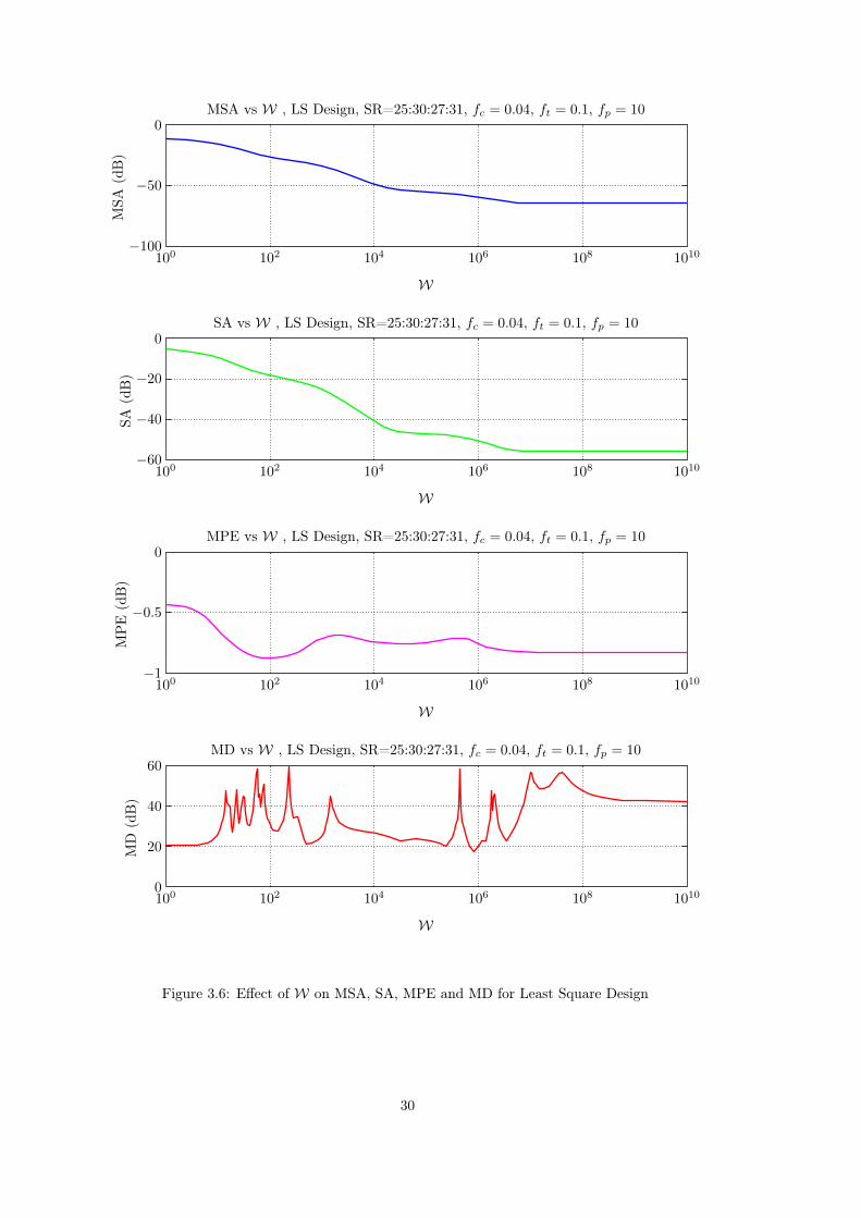
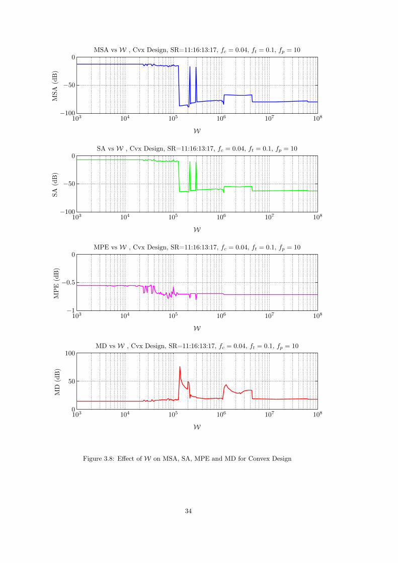
Figure 3.7 indicates the frequency response of the designed non-uniform MTI filter for differentweight factorsW and Table 3.2 gives the related performance criteria of the design. The effectof weight factor on the performance measures are plotted in Figure 3.8.

Stagger ratio used for the convex design is 11 : 16 : 13 : 17 (taken from [5]). As seen from theFigure 3.7, the effect of W on the stopband attenuation is similar to the least square design.The increase inW provides better attenuation in stopband whereas the maximum deviation inthe passband increases also. In order to obtain a more general opinion related to the effect ofweight factor, Figure 3.8 must be examined. It shows that the increase inW results in differenteffects on the performance measures. When the weight factor takes values between 104 and107, all the parameters change abruptly. However, four separate regions can be observed byexamining the stopband attenuation value. Stopband attenuation value takes different valuesthat stay constant for different W intervals. Mean passband error nearly shows a decreasingpattern whereas maximum deviation does not have a predictable behaviour.

Looking at the effect of weight factor on performance measures, it is reasonable to choose theweight factor similar to the least square design case. Once the required stopband attenuationis specified, the weight factor that gives the satisfactory stopband attenuation with smallermaximum deviation can be selected.

32

0 2 4 6 8 10 12−80

−60

−40

−20

0

20CVX Design, SR=11:16:13:17, fc = 0.04, ft = 0.1, fp = 10

fdoppler / PRFmax

|Hcvx(f

)|(dB)

W = 104

W = 105

W = 106

W = 107

0 0.02 0.04 0.06 0.08 0.1 0.12−80

−60

−40

−20


fdoppler / PRFmax

|Hcvx(f

)|(dB)

W = 104

W = 105

W = 106

W = 107

Figure 3.7: Frequency Response of Convex Design with Different W Values

Table 3.2: Performance Measures of Convex Design for Different W Values


10000 -14.540 -8.659 -0.614 17.464

100000 -15.470 -9.584 -0.664 18.310

1e+06 -77.987 -58.366 -0.612 25.309

1e+07 -79.187 -61.712 -0.635 26.876

33

103 104 105 106 107 108−100

−50

0MSA vs W , Cvx Design, SR=11:16:13:17, fc = 0.04, ft = 0.1, fp = 10

W

MSA

(dB)

103 104 105 106 107 108−100

−50

0SA vs W , Cvx Design, SR=11:16:13:17, fc = 0.04, ft = 0.1, fp = 10

W

SA(dB)

103 104 105 106 107 108−1

−0.5

0MPE vs W , Cvx Design, SR=11:16:13:17, fc = 0.04, ft = 0.1, fp = 10

W

MPE

(dB)

103 104 105 106 107 1080

50

100MD vs W , Cvx Design, SR=11:16:13:17, fc = 0.04, ft = 0.1, fp = 10

W

MD

(dB)

Figure 3.8: Effect of W on MSA, SA, MPE and MD for Convex Design

34

3.5 Min-Max Design

In this section, we examine the min-max filter design method for non-uniform MTI filterdesign. The min-max filter design aims to select the filter coefficients to minimize the maximumdeviation from the desired response in the passband. This method is different than the twoprevious methods. The earlier methods have a single optima which is the global one while thisone has many local maximas. Therefore, this method requires a good initial filter coefficientset for a satisfactory performance. It is therefore necessary to experiment with different initialfilter weights to determine the parameters that satisfy the required specifications. From theconstraints perspective, this filter design also based on the minimization of the maximumpassband ripple and maximization of the stopband attenuation. The optimization problem ofthe min-max design can be stated as follows

minimize δ

subject to |Hmm(f, αi)| ≤ δ, f ∈ [0, fc], αi ∈ R, i ∈ N0

|1− |Hmm(f, αi)|| ≤ Wδ, f ∈ [ft, fp], αi ∈ R, i ∈ N0

N−1∑

n=0

αn = 0, α ∈ R

(3.27)

Here Hmm(f, αi) is the frequency response of the min-max filter and the variable δ shows themaximum deviation from the desired characteristics (for W = 1). The goal in this designis to minimize the maximum deviation from the desired highpass characteristic. The firstand second constraints enforce the magnitude deviation be smaller than δ (for W = 1) in thedesignated bands. The third constraint guarantees that the min-max design has a null at DCfrequency.

Different from the LS design, there is no closed form mathematical relation from which theoptimal min-max filter coefficients can be retrieved. The optimization has to be done numer-ically. The numerical implementation of the optimization problem requires the discretizationof frequency band into a dense set of frequency points. Therefore, the constraints given in(3.27) are not evaluated for a continuum of points; but for a finitely many number of points.

Similar to the convex design, a weight factor W is introduced to establish a trade-off betweenclutter attenuation and passband ripple objectives. It should also be noted that the min-maxproblem examined here is focused on minimizing the maximum deviation of the magnituderesponse from the desired response.

Figure 3.9 indicates the obtained frequency response for different weight factors and Table 3.3gives the related performance measures of the design. The effect of weight factor, is given inFigure 3.10.

In these figures, the initial filter coefficients are kept constant and binomial coefficients areused in order to see the effect of the weight factor W individually. The stagger ratio of12 : 16 : 13 : 18 is used (taken from [38]). When the Figure 3.9 is examined, W indicates thesame effects as in least square and the convex designs. Larger values of W result in increasein stopband attenuation and passband ripple. However, different from the previous designs,maximum deviation does not have a monotonous increase or decrease characteristic. To get amore general idea, it is necessary to examine the effect of W in a much wider interval. Figure3.10 indicates the effect of W on the performance parameters. Examination of the figure

35

indicates that stopband attenuation parameters show a continuous increase whereas passbandripple fluctuates rapidly. In order to select the weight factor that gives a reasonable responsein terms of stopband attenuation and passband ripple, smaller maximum deviation value mustbe selected for specified stopband attenuation.

It is important to remember that Figures 3.9 and 3.10 are plotted by using the same initial filtercoefficients. Since the min-max optimization problem has local optima, it is necessary to seethe effect of the initial filter coefficients on the response of the min-max sensed designed non-uniform MTI filter. Therefore, min-max design is evaluated with different initial coefficientsets which are selected randomly. Obtained results are presented in Figure 3.11, 3.12 andTable 3.4

36

0 1 2 3 4 5 6 7 8 9 10−100

−80

−60

−40

−20

0

20Min-Max Design, SR=12:16:13:18, fc = 0.05, ft = 0.2, fp = 10

fdoppler / PRFmax

|Hmmx(f

)|(dB)

W =260W =790W =3510W =5590

0 0.01 0.02 0.03 0.04 0.05 0.06 0.07 0.08 0.09 0.1−100

−80

−60

−40

−20


fdoppler / PRFmax

|Hmmx(f

)|(dB)

W =260W =790W =3510W =5590

Figure 3.9: Frequency Response of Min-Max Design with Different W Values

Table 3.3: Performance Measures of Min-Max Design for Different W Values


260 -55.042 -50.697 -6.285 28.071

790 -63.927 -60.375 -0.577 17.535

3510 -78.101 -73.861 -7.224 25.245

5590 -78.861 -76.513 -14.918 31.869

37

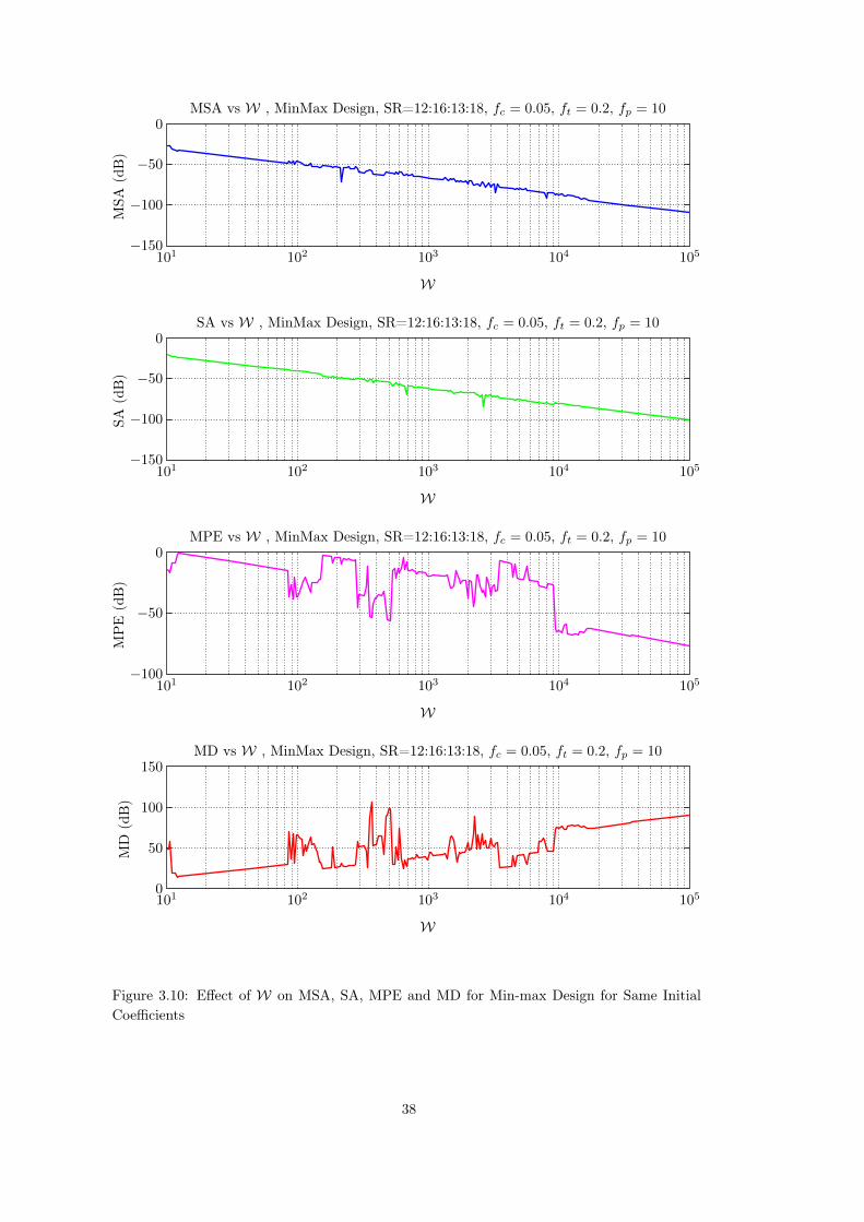
101 102 103 104 105−150

−100

−50

0MSA vs W , MinMax Design, SR=12:16:13:18, fc = 0.05, ft = 0.2, fp = 10

W

MSA

(dB)

101 102 103 104 105−150

−100

−50

0SA vs W , MinMax Design, SR=12:16:13:18, fc = 0.05, ft = 0.2, fp = 10

W

SA(dB)

101 102 103 104 105−100

−50

0MPE vs W , MinMax Design, SR=12:16:13:18, fc = 0.05, ft = 0.2, fp = 10

W

MPE

(dB)

101 102 103 104 1050

50

100

150MD vs W , MinMax Design, SR=12:16:13:18, fc = 0.05, ft = 0.2, fp = 10

W

MD

(dB)

Figure 3.10: Effect of W on MSA, SA, MPE and MD for Min-max Design for Same InitialCoefficients

38

Figure 3.11 indicates the response of min-max filter with four different initial coefficient setsand same weight factor. It is seen that several values in terms of stopband attenuation andpassband ripple are obtained. This indicates the importance of the effect of the initial filtercoefficients on the min-max design. Importance of the selection of the initial filter coefficientsare derived from the nature of the min-max design, since the min-max design algorithm seeksthe minimum deviation near the initial filter coefficient values. To see the effects of the initialfilter coefficient on the performance measures, 300 different initial conditions are evaluatedand the corresponding performance parameters are plotted in Figure 3.12.

Min-max design requires more computation compared to the previous least square and convexdesign methods. Initial filter coefficients and the weight factor must be selected appropriatelyin order to obtain the required response in terms of stopband attenuation and the passbandripple. The taken approach for the min-max design of non-uniform MTI filter requires twophases. First, the weight factor is determined according to the required stopband attenuationby using the binomial coefficients as the initial filter coefficients. After the weight factor selec-tion, different initial conditions for specified number of iterations are tried and the coefficientsthat give the minimum deviation in the passband are selected. Using this approach four filtersare designed and obtained results are presented in Figure 3.13. Stopband attenuation boundfor these four filters are selected as 45 dB, 45 dB, 60 dB and 70 dB respectively. Obtainedperformance parameters are given in Table 3.5. Using this approach, it is possible to obtaindesired stopband attenuation with improved maximum deviation by determining the initialfilter coefficients and weight factor.

39

0 1 2 3 4 5 6 7 8 9 10−100

−80

−60

−40

−20

0

20Min-Max Design, SR=12:16:13:18 ,W = 3510, fc = 0.05, ft = 0.2, fp = 10

fdoppler / PRFmax

|Hmmx(f

)|(dB)

i.c.v = ξ

i.c.v = ζ

i.c.v = υ

i.c.v = ι

0 0.01 0.02 0.03 0.04 0.05 0.06 0.07 0.08 0.09 0.1−100

−80

−60

−40

−20


fdoppler / PRFmax

|Hmmx(f

)|(dB)

i.c.v = ξ

i.c.v = ζ

i.c.v = υ

i.c.v = ι

Figure 3.11: Frequency Response of Min-Max Design for Different Initial Conditions with theSame W Values

Table 3.4: Performance Measures for Min-max Design for Different Initial Filter Coefficientswith Same W Values

Initial Coefficient Vector (i.c.v) MSA (dB) SA (dB) MPE (dB) MD (dB)

ξ = [-0.53 -0.26 1.72 -1.09 0.16] -32.044 -23.682 -0.566 14.132

ζ = [0.57 0.14 2.22 -0.52 -2.42] -29.156 -20.073 -0.561 11.315

υ = [0.52 1.20 -1.12 0.74 -1.34] -71.135 -66.891 -0.614 18.262

ι = [0.18 0.04 0.53 -0.89 0.15] -59.852 -53.433 -0.616 20.107

40

0 50 100 150 200 250 300−100

−50

0MSA vs i.c.v , MinMax Design, SR=12:16:13:18, fc = 0.05, ft = 0.2, fp = 10

Number of i.c.v

MSA

(dB)

0 50 100 150 200 250 300−100

−50

0

50SA vs i.c.v , MinMax Design, SR=12:16:13:18, fc = 0.05, ft = 0.2, fp = 10

Number of i.c.v

SA(dB)

0 50 100 150 200 250 300−1

−0.5

0MPE vs i.c.v , MinMax Design, SR=12:16:13:18, fc = 0.05, ft = 0.2, fp = 10

Number of i.c.v

MPE

(dB)

0 50 100 150 200 250 3000

20

40

60MD vs i.c.v , MinMax Design, SR=12:16:13:18, fc = 0.05, ft = 0.2, fp = 10

Number of i.c.v

MD

(dB)

Figure 3.12: Effect of Initial Filter Coefficients on Performance Measures of Min-Max Designfor Same W Values

41

0 1 2 3 4 5 6 7 8 9 10−100

−80

−60

−40

−20

0

20MinMax Design, SR=12:16:13:18, W = 3510, fc = 0.05, ft = 0.2, fp = 10

fdoppler / PRFmax

|Hmmx(f

)|(dB)

i.c.v = ξ

i.c.v = ζ

i.c.v = υ

i.c.v = ι

0 0.01 0.02 0.03 0.04 0.05 0.06 0.07 0.08 0.09 0.1−100

−80

−60

−40

−20


fdoppler / PRFmax

|Hmmx(f

)|(dB)

i.c.v = ξ

i.c.v = ζ

i.c.v = υ

i.c.v = ι

Figure 3.13: Min-Max Design for Different Stopband Attenuation Requirement with DifferentInitial Conditions and W Values

Table 3.5: Performance Measures of Min-Max Design for Different Stopband AttenuationRequirement with Different Initial Conditions and W Values

Initial Coefficient Vector (i.c.v) MSA (dB) SA (dB) MPE (dB) MD (dB)

ξ = [-1.92 0.63 0.75 0.21 0.33] -46.910 -42.645 -0.691 15.978

ζ = [-0.94 -0.65 0.28 -1.13 2.44] -47.361 -44.824 -0.671 24.601

υ = [0.96 -0.34 -0.17 0.62 -1.06] -64.175 -61.705 -0.613 17.565

ι = [-1.52 -1.07 -3.07 0.52 5.14] -71.357 -67.105 -0.614 18.488

42

3.6 Numerical Comparison with Selected Filter Designs

To this point designed filters are compared individually with different weight factors and initialcoefficient sets. In this section filter designs will be compared among themselves and also withthe similar filters in the literature.

3.6.1 Binomial Filter

As explained in previous chapter, Binomial filter is a filter that is derived by cascading singlecancellers. These are simple FIR filters whose coefficients are selected as binomial numberswith alternating signs that are given by

wi = (−1)i−1N !

(N − i+ 1)!(i− 1)!, i = 1, 2, . . . , N + 1 (3.28)

where N is the order of the filter.

Binomial filters are widely used filters for performance comparison of MTI filters in the liter-ature.

3.6.2 Prinsen’s Filter

Prinsen developed a simple algorithm for staggered PRF MTI filters [11]. Design is based onthe requirement for the maximally flat stopband characteristic at zero frequency. The filterdesign also a generalization to the Binomial filter. FIR filter equation for the MTI design isgiven in (3.29).

y(f) =

N−1∑

n=1

wnej2πftn (3.29)

where w0, ..., wN−1 are filter coefficients and t0, ..., tN−1 are the sampling times.

Theory of the design relies on making the first M coefficients of the Taylor series expansionof the filter response near zero frequency to be zero.

The Taylor expansion of y(f) around f = 0 is given in following equations.

y(f) = y(0) +y′(0)

1!f +

y′′(0)

2!f2 + . . . (3.30)

y(k)(0) = (j2π)kN−1∑

n=0

tknwn, k = 0, 1, 2, . . . (3.31)

Maximally flat stopband and a non-trivial solution requires that the first N − 1 coefficients ofy(k)(0), k = 0, . . . ,M − 1 in (3.31) to be zero. Matrix form of the N − 1 equations are givenas

Tw = −w0u1 (3.32)

43

where

T =

1 1 . . . 1

t1 t2 . . . tN−1...

.... . .

...tN−21 tN−22 . . . tN−2N−1

, w =

w1

w2

. . .

wN−2

, u1 =

1

0

. . .

0

T matrix is a Vandermonde matrix and T−1 exists since ti 6= tj for i 6= j. Simplified form ofthe equation is given in (3.33).

wi = −w0

N−1∏

n=1n 6=i

tntn − ti

i = 1, . . . , N − 1 (3.33)

Designed filters are compared with Binomial and Prinsen’s MTI filters under four differentcases.

In the first case, the stopband attenuation (SA) is fixed. In Figure 3.14, the desired stopbandattenuation value is selected as -60 dB. This means that, the magnitude of the filter responsesis designed to better than 60 dB at the cutoff frequency fc. By examining the performancemeasures given in Table 3.6, one can see that LS design does not provide the required attenu-ation. This is due to the stopband performance of the LS design. 56.228 dB is the maximumattenuation that LS design can achieve for the used stagger ratio. It must also be noted thatthe LS design has the smallest mean passband error.

If the performance of the CVX design is focused, it has good stopband attenuation and reason-able values in terms of passband ripple. The performance in stopband is related to the choiceof the weight factor. By choosing a different weight factor better values could be obtained forpassband ripple with decreased stopband attenuation performance.

The desired min-max design achieves least deviation value and provides required stopbandattenuation. Response of Prinsen’s filter is also satisfactory. Since it is designed for maximallyflat stopband response, it gives better attenuation values. However the passband performanceis not very satisfactory and it has large deviations from the ideal response. It has the worstmaximum deviation compared to other filter designs.

In the second case, cutoff frequency fc is reduced. Figure 3.15 indicates this case. As observed,all the responses are improved in terms of stopband attenuation and passband ripple. Itshould be noted that, the response of LS design is improved, but it does not provide samesuppression level of other designs except the Binomial filter. It is also eye catching that,maximum deviation of the CVX design is improved nearly 10 dB compared to the previouscase.

In the third case, a bigger cutoff frequency is examined. Figure 3.16 shows the response offilters when the cutoff frequency fc is selected as 0.08. Expectedly, stopband attenuationperformances of the filters are decreased. However passband performances do not worsen .On the contrary, better maximum deviation is obtained with min-max design.

The final case considers the response to the bigger velocity band. Figure 3.17 indicates theresponse of the filters when the passband bound is increased to ten times of the maximumPRF value. As compared with the Figure 3.14, Min-Max and CVX designs present betterresponses. However response of LS filter in terms of maximum deviation is degraded with

44

respect to the first case. Therefore, it can be concluded that the usage of wider velocity bandexhibits different effects on the performance of the filter designs.

45

0 1 2 3 4 5 6 7 8 9 10−100

−80

−60

−40

−20

0

Comparison of Designs, SR=14:16:17:19:16, fc = 0.05, ft = 0.5, fp = 8

fdoppler / PRFmax

Magnitude

(dB)

LsCvxMinmaxPrinsenBinom

0 0.01 0.02 0.03 0.04 0.05 0.06 0.07 0.08 0.09 0.1−100

−80

−60

−40

−20


fdoppler / PRFmax

Magnitude

(dB)


Figure 3.14: Comparison of Designed Filters with Binomial and Prinsen’s Filter with SameStopband Attenuation Requirement

Table 3.6: Performance Measures for Comparison of Designed Filters with Binomial andPrinsen’s Filter with Same Stopband Attenuation Requirement

Designs MSA (dB) SA (dB) MPE (dB) MD (dB)

Ls -65.918 -56.228 -1.128 22.974

Cvx -84.256 -68.740 -0.807 31.856

Min-Max -71.762 -68.536 -0.796 19.944

Prinsen -81.606 -67.280 -0.800 34.047

Binom -45.688 -40.175 -0.798 24.773

46

0 1 2 3 4 5 6 7 8 9 10−100

−80

−60

−40

−20

0


fdoppler / PRFmax

Magnitude

(dB)


0 0.01 0.02 0.03 0.04 0.05 0.06−100

−80

−60

−40

−20


fdoppler / PRFmax

Magnitude

(dB)


Figure 3.15: Comparison of Designed Filters with Binomial and Prinsen’s Filter with SmallerCutoff Frequency

Table 3.7: Performance Measures for Comparison of Designed Filters with Binomial andPrinsen’s Filter with Smaller Cutoff Frequency


Ls -68.928 -60.051 -0.768 20.098

Cvx -102.017 -87.380 -0.806 25.971

Min-Max -77.504 -83.057 -0.863 22.698

Prinsen -98.145 -86.868 -0.800 34.047

Binom -49.776 -43.951 -0.798 24.773

47

0 1 2 3 4 5 6 7 8 9 10−100

−80

−60

−40

−20

0


fdoppler / PRFmax

Magnitude

(dB)


0 0.02 0.04 0.06 0.08 0.1 0.12 0.14 0.16−100

−80

−60

−40

−20


fdoppler / PRFmax

Magnitude

(dB)


Figure 3.16: Comparison of Designed Filters with Binomial and Prinsen’s Filter with BiggerCutoff Frequency

Table 3.8: Performance Measures for Comparison of Designed Filters with Binomial andPrinsen’s Filter with Bigger Cutoff Frequency


Ls -62.313 -52.694 -0.762 24.395

Cvx -64.628 -57.884 -0.803 31.225

Min-Max -52.152 -47.638 -0.782 15.648

Prinsen -61.969 -46.941 -0.800 34.047

Binom -41.948 -35.948 -0.798 24.773

48

0 1 2 3 4 5 6 7 8 9 10−100

−80

−60

−40

−20

0


fdoppler / PRFmax

Magnitude

(dB)


0 0.01 0.02 0.03 0.04 0.05 0.06 0.07 0.08 0.09 0.1−100

−80

−60

−40

−20


fdoppler / PRFmax

Magnitude

(dB)


Figure 3.17: Comparison of Designed Filters with Binomial and Prinsen Filter’s with LargerVelocity Band

Table 3.9: Performance Measures for Comparison of Designed Filters with Binomial andPrinsen’s Filter with Larger Velocity Band


Ls -65.499 -54.759 -1.032 23.855

Cvx -76.607 -66.319 -0.913 19.634

Min-Max -68.512 -63.361 -0.833 15.187

Prinsen -80.774 -66.461 -0.891 34.104

Binom -45.538 -40.038 -0.901 24.773

49

CHAPTER 4

CLUTTER SUPPRESSION PERFORMANCE OFFILTER DESIGNS

In this chapter clutter is taken into account for designing optimal staggered MTI filters. First,definition of the clutter and properties of the clutter covariance matrix are given. Second,optimal filters are studied for different types of clutter PSD’s. Later, performances of thefilter designs are compared according to MTI improvement factor and a modified min-maxdesign is presented. Finally, time varying filter concept is explained and obtained results arediscussed.

4.1 Characteristics of Clutter

Clutter is defined as non-wanted interference from land, sea or weather. Return from these,can block the target component of the radar echo signal. Therefore, it is important to rejectclutter in radar signal processor units. In most cases the rejection of the clutter is used as aperformance index such as clutter attenuation and subclutter visibility.

For MTI filter performance analysis, the effect of clutter is put into consideration by usingclutter covariance matrix or clutter power spectrum density (PSD). Transformation betweenthese metrics are carried out with Fourier transformation.

Widely used model for the clutter PSD is Gaussian Model with zero mean Doppler frequency([3]):

C(f) =Pc√2πσg

exp

(−f22σ2

g

)(4.1)

Here Pc is the clutter power, f is the Doppler frequency and σg is the standard deviation ofthe clutter spectrum. An example of Gaussian Clutter model for several σg values are givenin Figure 4.1.

Using the power spectral model, the elements of the normalized clutter covariance matrix canbe found by

Rij =

∫ ∞

−∞C(f)ej2πf(ti−tj)df

= e−2π2σ2

g(ti−tj)2

(4.2)

51

−π −π/2 0 π/2 π0

0.2

0.4

0.6

0.8

1Normalized

Magnitude

Frequency (rad/sec)

Gaussian Clutter Power Spectrum Model

σg = 0.3

σg = 0.4

σg = 0.5

Figure 4.1: Gaussian Clutter Power Spectrum Density Model

Calculation of the optimal MTI filters is based upon clutter covariance matrix. Hsiao [13]shows that elements of the eigenvector that corresponds to the minimum eigenvalue of theclutter covariance matrix, are the coefficients of the optimum MTI filter.

Another optimum filter design comes from the matched filtering concept. The weights are cal-culated for each transmitted signal component in the sense of matching the received waveform.Optimal filter weights for each transmitted pulse are given by

wopt = R−1s (4.3)

Here wopt is the coefficient vector of optimum filter weights and s is the signal vector. Figure4.2 illustrates the performance comparison of optimal filters with different clutter PSD values.Here, optimal filter-2 represents the eigenfilter method of Hsiao’s (the filter corresponds toeigenvector of Rc with the smallest eigenvalue), whereas optimal filter-1 illustrates the matchfilter type optimal filter. The first sub figure is plotted with a Gaussian clutter PSD and thesecond sub figure is plotted with a Gaussian clutter PSD model with a large Doppler spread.For the first case, optimal filters show the same performance, whereas in the second caseoptimal filter-1 shows better response for all Doppler frequencies. It must be noted that theoptimal filter-1 is unique for each frequency as seen from (4.3), whereas the optimal filter-2 isthe same for all frequencies.

52

0 0.1 0.2 0.3 0.4 0.5 0.6 0.7 0.8 0.9 10

10

20

30

40

50

60IF vs Normalized Frequency,Gauss Clutter, σg =0.04


IF(dB)

Optimum Filter-1Optimum Filter-2

0 0.1 0.2 0.3 0.4 0.5 0.6 0.7 0.8 0.9 10

10

20

30

40

50

60IF vs Normalized Frequency,Gauss Clutter, σg =0.06


IF(dB)

Optimum Filter-1Optimum Filter-2

Figure 4.2: Comparison of Optimum MTI Filters with Different Clutter PSD’s

53

4.2 Comparison of Designed Filters with Optimal MTI Filter

In the previous section, designed filters are compared in terms of magnitude response. In thissection, the filters are compared in terms of MTI improvement factors. MTI improvementfactor of the corresponding FIR filter designs can be calculated as follows;

IF =wHRsw

wHRcw(4.4)

where the variables w, Rc and Rs represent weight vector, clutter covariance matrix andsignal covariance matrix respectively.

The comparisons related to improvement factor in the following figures and chapters, the effectof Doppler spread of clutter is investigated. The used clutter models and corresponding valuesof parameters are given in Table 4.1.

Table 4.1: Used Clutter Models and Related Values of Parameters

Antenna Type Stationary Antenna Rotary Antenna

Clutter Models Gaussian Clutter Gaussian Clutter

Doppler Spread (fdoppler/PRFmax) 0.02-0.08 0.02-0.08

SNR (dB) 10 10

CNR (dB) 50 50

Azimuth Beamwidth (◦) - 1.7

Antenna Rotation Period (rpm) - 40

For the sake of comparison, the frequency responses of the designs are presented first. Figure4.3 indicates the frequency responses of the designed filters with Prinsen’s filter for the staggerratio of 36 : 45 : 39 : 48 : 42. Table 4.2 presents the performance measures. If the figure isexamined, it is seen that the responses of the filters show similar passband characteristic exceptfrom the maximum deviation value and stopband responses.

In Figure 4.4 improvement factor for each filter in Figure 4.3 is plotted with the assumption ofthe Gaussian clutter PSD. It is seen that all the filters have almost identical improvement factorvalues in the passband. These values are given in Table 4.3. By comparing the improvementfactors and performance measures, it is possible to conclude that mean stopband attenuation(MSA) criteria is closely linked to the improvement factor performance of the filters.

In Figure 4.5 improvement factors for all filters are plotted with different type of clutter model.In this case a Gaussian clutter with larger spread is used. For this case, the optimal filterresponse shows different characteristic compared to other filters. All the other filters achievevery similar improvement factors whereas the performance of them differs from the optimalfilter considerably. Prinsen’s filter and designed filters according to the performance measuresdo not provide an improvement factor close to the optimal case.

The decrease in the improvement factor values and associated performance measures constitutethe possibility of designing another type of non-uniform MTI filter with better improvement

54

factor. The idea is investigated in the following subsection and another design method isdeveloped by modifying the min-max design according to MTI improvement factor of optimalfilter.

55

0 1 2 3 4 5 6 7 8 9 10−80

−60

−40

−20

0

20Comparison of Designs, SR=36:45:39:48:42, fc = 0.07, ft = 0.2, fp = 10

fdoppler / PRFmax

Magnitude

(dB)

LsCvxMin-MaxPrinsen

0 0.02 0.04 0.06 0.08 0.1 0.12 0.14−80

−60

−40

−20


fdoppler / PRFmax

Magnitude

(dB)

LsCvxMin-MaxPrinsen

Figure 4.3: Frequency Response Comparison of Designed Filters with Prinsen’s Filter

Table 4.2: Performance Measures for Comparison of Designed Filters with Prinsen’s Filter


Ls -72.682 -82.032 -0.532 22.603

Cvx -69.843 -69.549 -0.529 25.691

Minmax -75.708 -62.296 -0.533 22.670

Prinsen -67.130 -53.172 -0.525 36.056

56

0 2 4 6 8 10 120

10

20

30

40

50

60

70

IF vs Normalized Freq., Stagger Ratio 36:45:39:48:42, σg =0.03

Normalized Frequency (fd / PRFmax)

IF(dB)

OptLsCvxMin-MaxPrinsen

0 0.02 0.04 0.06 0.08 0.1 0.12 0.140

10

20

30

40



IF(dB)


Figure 4.4: Improvement Factor Comparison of Designed Filters with Prinsen’s Filter withGaussian Clutter PSD

Table 4.3: Improvement Factor Values for Comparison of Designed Filters with Prinsen’sFilter with Gaussian Clutter PSD

Optimum Ls Cvx Minmax Prinsen

Improvement Factor (dB) 66.555 63.275 63.463 61.975 58.120

57

0 2 4 6 8 10 120

10

20

30

40

50

60IF vs Normalized Freq., Stagger Ratio 36:45:39:48:42, fc =0.07


IF(dB)


0 0.02 0.04 0.06 0.08 0.1 0.12 0.140

5

10

15



IF(dB)


Figure 4.5: Improvement Factor Comparison of Designed Filters with Prinsen’s Filter withGaussian Clutter PSD with Larger Doppler Spread

Table 4.4: Improvement Factor Values for Comparison of Designed Filters with Prinsen’sFilter with Gaussian Clutter PSD with Larger Doppler Spread

Optimum Ls Cvx Minmax Prinsen

Improvement Factor (dB) 45.159 39.362 39.702 38.849 37.667

58

4.3 Min-Max Filter Design with Optimum Improvement Factor

In this section min-max filter design is modified for the purpose of obtaining a non-uniformMTI filter based on the MTI improvement factor of the optimum filter. First, a frequencyinterval is taken and the improvement factor of the optimum filter is calculated for eachfrequency value in the frequency interval of interest. Later, filter coefficients are optimized toprovide the nearest improvement factor to optimum filter’s using a min-max sense approach.

The optimization equation of the corresponding design is given in (4.5)

minwd,f

(Iopt − Id) = minwd,f

(wH

optRswopt

wHoptRxwopt

− wHd Rswd

wHd Rxwd

)(4.5)

where

• Iopt : Optimum filter interference improvement factor

• Id : Designed filter interference improvement factor

• wopt : Optimum filter coefficient vector

• wd : Designed filter coefficient vector

• Rx : Interference covariance matrix (Rx = Rc + Rn = Rc + σ2nI)

• Rs : Signal covariance matrix (Rs = E{s(θ)sH(θ)})

The steps of near optimum filter design algorithm can be listed as follows

• Determine interpulse periods

• Calculate optimum filter improvement factor for each frequency value in the frequencyinterval of interest

• Determine initial value of filter coefficients for the near optimum filter design

• Calculate the filter coefficients that give the most near value to the optimum filterimprovement factor

Min-max filter design with the optimum improvement factor is compared with previously de-signed filters for two cases. Figure 4.6 indicates the magnitude of the frequency responses ofthe filters. All the filters show same passband response whereas they have different stopbandattenuation values. The new approach of min-max design named as, MinMax-IF, shows dif-ferent behavior compared to others since it is designed according to improvement factor ofoptimum filter. Other filters provide better response when the performance measures in Table4.5 are compared. The different behaviour is due to the value of the cutoff frequency of theMinmax-IF design. Since the weights are adjusted according to the optimum improvementfactor, corresponding cutoff frequency value can be different than the other filters.

Figure 4.7 indicates the comparison of the improvement factors for the Gaussian clutter powerspectral density. MinMax-IF design has better improvement factor value compared to other

59

filters. In Figure 4.8, the comparison of the improvement factors for the case of Gaussianclutter with larger spread is illustrated. For this case Minmax-IF filter has better improvementfactor compared to others for this case also. As seen from the obtained results, this filtergives improved response compared to others. One of the disadvantage of this design is therequirement of the optimal filter coefficients that depends upon the clutter covariance matrix.

60

0 1 2 3 4 5 6 7 8 9 10−100

−80

−60

−40

−20

0


fdoppler / PRFmax

Magnitude

(dB)

LsCvxMinmaxMinmax-IFPrinsen

0 0.01 0.02 0.03 0.04 0.05 0.06 0.07 0.08 0.09 0.1−100

−80

−60

−40

−20


fdoppler / PRFmax

Magnitude

(dB)

LsCvxMinmaxMinmax-IFPrinsen

Figure 4.6: Frequency Response Comparison of Minmax-IF Filter with Other Filter Designs

Table 4.5: Performance Measures of the Comparison of Minmax-IF Filter with Other FilterDesigns


Ls -82.962 -71.403 -0.860 25.820

Cvx -85.065 -70.810 -0.868 26.340

Minmax -81.992 -80.121 -0.866 23.588

Minmax-IF -67.136 -69.674 -0.909 42.753

Prinsen -83.291 -68.616 -0.891 33.425

61

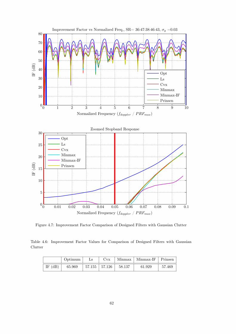
0 1 2 3 4 5 6 7 8 9 100

10

20

30

40

50

60

70

80Improvement Factor vs Normalized Freq., SR= 36:47:38:46:43, σg =0.03

Normalized Frequency (fdoppler / PRFmax)

IF(dB)

OptLsCvxMinmaxMinmax-IFPrinsen

0 0.01 0.02 0.03 0.04 0.05 0.06 0.07 0.08 0.09 0.10

5

10

15

20

25



IF(dB)


Figure 4.7: Improvement Factor Comparison of Designed Filters with Gaussian Clutter

Table 4.6: Improvement Factor Values for Comparison of Designed Filters with GaussianClutter

Optimum Ls Cvx Minmax Minmax-IF Prinsen

IF (dB) 65.969 57.155 57.126 58.137 61.929 57.469

62

0 1 2 3 4 5 6 7 8 9 100

10

20

30

40

50Improvement Factor vs Normalized Freq., SR= 36:47:38:46:43, σg =0.06


IF(dB)


0 0.02 0.04 0.06 0.08 0.1 0.12 0.14 0.16 0.18 0.20

5

10

15

20

25



IF(dB)


Figure 4.8: Improvement Factor Comparison of Designed Filters with Gaussian Clutter withLarger Doppler Spread

Table 4.7: Improvement Factor Values for Comparison of Designed Filters with GaussianClutter with Larger Doppler Spread

Optimum Ls Cvx Minmax Minmax-IF Prinsen

IF (dB) 37.193 30.051 30.055 30.309 32.785 30.092

63

4.4 Multiple Filter Design with Time Varying Coefficients

Multiple filter design is the use of time varying weights for the processing of successivelytransmitted pulses. Shrader [2] states that "The improvement factor limitation caused bypulse to pulse staggering can be avoided by the use of time varying weights in the cancellerforward paths instead of binomial weights." Following multiple filter discussion considers thiscase and compares the responses with respect to time constant weights.

Multiple filter design can be described as the usage of more than one set of filter coefficientsfor the processing of transmitted pulses. In the previous chapters a single filter with N + 1

filter weights are used for processing of one period with N staggers. Usage of multiple filtersmeans the processing of received pulses with more than one filters. Structure of the multiplefilter processing is indicated in Figure 4.9.

Lets assume thatN+L pulses are transmitted for the MTI operation, when the stagger patternincludes N stagger periods. In time invariant single filter case, an MTI filter is designed withN + 1 coefficients and transmitted pulses are processed successively using this filter. In timevarying weights case, multiple MTI filters are designed with N + 1 coefficients. That is pulsesfrom 1 to N are processed by the first filter, 2 to N + 1 are processed by the second filterand so on. Processing of N +L pulses with multiple filters can be thought as summing of thepower outputs of the filters in order to obtain the total response of the multiple filter system.For L number of filters the total power output can be written as

|H(f)|2 = |H1(f)|2 + |H2(f)|2 + |H3(f)|2 + . . .+ |HL(f)|2 (4.6)

where |Hi(f)|2 represents the power output of each filter in multiple filter system. When thefilter responses put in (4.6), following equation can be obtained.

64

0 1 2 N N+1 N+2 N+LT1 T2 ... TN T1 ...

Filter 1

Filter 2

Normal Filtering

inputDelayT1

DelayT2

DelayT3

... DelayTN

w0 × w1 × w2 × w3 × ... wN ×∑

output

Multiple Filtering

inputDelayT1

DelayT2

DelayT3

... DelayTN+1

α0 × α1 × α2 × α3 × ... αN ×∑

inputDelayT2

DelayT3

DelayT4

... DelayTN+2

β0 × β1 × β2 × β3 × ... βN ×∑

inputDelayTL

DelayTL+1

DelayTL+2

... DelayTN+L

γ0 × γ1 × γ2 × γ3 × ... γN ×∑

......

...

∑output

Filter 1

Filter 2

Filter L

|.|2

|.|2

|.|2

Figure 4.9: Processing of Received Pulses with Multiple Filter Structure with Time VaryingCoefficients

65

|H(f)|2 = |N∑

i=1

αi exp (−j2πfti)|2 + |N+1∑

i=2

βi exp (−j2πfti)|2 + . . .

. . .+ |L∑

i=L−N+1

γi exp (−j2πfti)|2 (4.7)

where N is the number of staggers, L is the number of pulses processed, αi’s are filter weightsof the first filter, βi’s are the filter weights of second filter, . . . , and γi’s are the filter weightsof Lth filter.

The main idea for the multiple filtering is the adaptation of the MTI filters for the specificstagger intervals. For example, lets consider the case when the stagger ratio of 8 : 9 : 10 is usedand 7 pulses are transmitted with staggers 8 : 9 : 10 : 8 : 9 : 10. That is 8 : 9 : 10 sequenceis repeated twice. According to the single filter approach, an MTI filter with 4 weights isdesigned with 8 : 9 : 10 stagger pattern. Let’s assume that these weights are α1, α2, α3 andα4. Then, these are used as follows for the processing of 7 pulses. The group of successivestaggers of 8 : 9 : 10, 9 : 10 : 8, 10 : 8 : 9, and 8 : 9 : 10 are processed by this filter. Whenthe multiple filtering approach is used, 4 MTI filters are designed based on stagger sets of8 : 9 : 10, 9 : 10 : 8 and 10 : 8 : 9 and 8 : 9 : 10. First MTI filter with weight vector α is usedto process 8 : 9 : 10, second MTI filter with weight vector β is used to process 9 : 10 : 8, thirdMTI filter with weight vector γ is used to process 10 : 8 : 9 and fourth MTI filter with weightvector η is used to process 8 : 9 : 10. The matrix representation that gives the output of eachMTI filter is indicated in (4.8)

O1

O2

O3

O4

=

α1 α2 α3 α4 0 0 0

0 β1 β2 β3 β4 0 0

0 0 γ1 γ2 γ3 γ4 0

0 0 0 η1 η2 η3 η4

P1

P2

P3

P4

P5

P6

P7

(4.8)

where P1 to P7 are the input pulses and O1 to O4 are MTI filter outputs. O1 is the outputof MTI using the first 4 pulses. These pulses are seperated by T1, T2, T3 seconds as shown intop part of Figure 4.9. O2 is the output using the successive 4 pulses starting from 2nd pulse.These pulses are separated by T2, T3, T4 seconds.

Assuming the target has a Doppler of frequency of fd, then Pk in equation (4.8) becomesas Pk = ej2πfdtk , as before. Then O1 =

∑Nk=1 αke

j2πfdtk , O2 =∑N+1k=2 βk−1e

j2πfdtk , O3 =∑N+2k=3 γk−2e

j2πfdtk and O4 =∑N+3k=4 ηk−3e

j2πfdtk .

To investigate the performance of multiple filtering, firstly non-uniform filter designs are im-plemented as time invariant filters. Figure 4.10 indicates the single filters for the stagger ratioof 16 : 20 : 17 : 22. Response of the designed filters is similar to each other and they exhibit60 dB average stopband attenuation and 20 dB maximum deviation in the passband. Table4.8 indicates the performance measures.

Figure 4.11 illustrates the improvement factors of the designed filters in Figure 4.10. All the

66

filters achieve similar improvement factors. These are given in Table 4.9. Up to this point,there is no difference with respect to the earlier comparisons. Now these designed filters willbe used for multiple filtering.

Figure 4.12 indicates the power response of the multiple filters when the designed filters inFigure 4.10 are used for to set-up of multiple filtering. Figure 4.13 indicates the improvementfactor for multiple filters. The stagger ratio utilized is 16 : 20 : 17 : 22 : 16 : 20 : 17. It is seenfrom the figure that, all the filters exhibit same response. Table 4.10 shows the performanceparameters and they are nearly same for all the filters. It must be noted here that filters havebetter frequency responses for the stagger ratio of 16 : 20 : 17 : 22. However when they areused for stagger ratios 20 : 17 : 22 : 16, 17 : 22 : 16 : 20 and 22 : 16 : 20 : 17, the responsebecome worse and all the filters show the same power response. The effect can be seen moreclearly if the filter responses are examined individually. Figure 4.14 and 4.15 indicate thefilter responses for passband and stopband for each stagger pattern cases. As it is seen, theperformance of the filters is satisfactory for the first sub plot. However, the performance ofthe filters decrease in terms of stopband attenuation for other sub-plots. Table 4.12, 4.13,4.14 and 4.15 indicate the performance parameters for single filters with stagger ratios of16 : 20 : 17 : 22, 20 : 17 : 22 : 16, 17 : 22 : 16 : 20 and 22 : 16 : 20 : 17 respectively.

Figure 4.16 and 4.17 indicate the passband and stopband of the filters designed for eachspecific stagger ratios. It is seen from the Tables 4.16, 4.17, 4.18 and 4.19 that better stopbandattenuation values are obtained (nearly 60 dB) when the time varying filters are designed foreach stagger pattern.

Figure 4.18 and 4.19 indicate power response and improvement factors of multiple filters withtime varying coefficients for the stagger ratio of 16 : 20 : 17 : 22 : 16 : 20 : 17. As it is observed,stopband attenuation of the multiple filters is greater than time invariant coefficient filters. Inother words, if a single MTI filter is designed for each sub-stagger group and used in multiplefilter structure, stopband attenuation performance do not degrade as compared to the singletime invariant MTI filter.

67

0 2 4 6 8 10 12−80

−60

−40

−20

0

20Comparison of Designs, SR=16:20:17:22, fc = 0.05, ft = 0.5, fp = 10

fdoppler / PRFmax

Magnitude

(dB)

LsCvxMin-MaxPrinsenBinom

0 0.02 0.04 0.06 0.08 0.1 0.12−80

−60

−40

−20


fdoppler / PRFmax

Magnitude

(dB)


Figure 4.10: Frequency Response of Designed Filters for Stagger Ratio 16:20:17:22 (SingleFilter)

Table 4.8: Performance Measures of Designed Filters for Stagger Ratio 16:20:17:22


Ls -65.480 -64.418 -0.023 22.601

Cvx -65.520 -57.212 -0.020 19.102

Min-Max -65.004 -63.755 -0.009 19.804

Prinsen -63.915 -54.892 -0.016 31.950

Binom -34.498 -30.181 -0.013 28.499

68

0 2 4 6 8 10 120

10

20

30

40

50

60Improvement Factor vs Normalized Freq., Stagger Ratio 16:20:17:22


IF(dB)

OptLsCvxMinmaxPrinsenBinom

0 0.05 0.1 0.15 0.2 0.250

5

10

15

20

25

30

35



IF(dB)


Figure 4.11: Improvement Factor Plots of Designed Filters for Stagger Ratio 16:20:17:22(Single Filter)

Table 4.9: Improvement Factor Values of Designed Filters for Stagger Ratio 16:20:17:22

Optimum Ls Cvx Minmax Prinsen Binom

IF (dB) 45.769 40.487 40.061 40.530 39.921 30.329

69

0 2 4 6 8 10 12−80

−60

−40

−20

0

20Comparison of Designs, SR=16:20:17:22:16:20:17, fc = 0.05, ft = 0.5, fp = 10

fdoppler / PRFmax

Total

Pow

erOutpu

t(dB)


0 0.02 0.04 0.06 0.08 0.1 0.12−80

−60

−40

−20


fdoppler / PRFmax

Total

Pow

erOutpu

t(dB)


Figure 4.12: Total Power Response of Designed Time Invariant Single Filters for Stagger Ratio16:20:17:22:16:20:17 (Multiple Filter)

Table 4.10: Performance Measures of Total Power Response of Designed Filters for StaggerRatio 16:20:17:22:16:20:17


Ls -30.399 -26.089 -0.025 8.422

Cvx -30.437 -26.097 -0.024 8.337

Min-Max -30.440 -25.920 -0.024 8.027

Prinsen -30.449 -26.031 -0.024 8.191

Binom -32.598 -28.116 -0.024 8.191

70

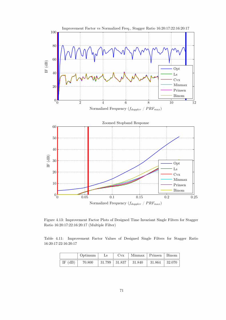
0 2 4 6 8 10 120

20

40

60

80

100Improvement Factor vs Normalized Freq., Stagger Ratio 16:20:17:22:16:20:17


IF(dB)


0 0.05 0.1 0.15 0.2 0.250

10

20

30

40

50



IF(dB)


Figure 4.13: Improvement Factor Plots of Designed Time Invariant Single Filters for StaggerRatio 16:20:17:22:16:20:17 (Multiple Filter)

Table 4.11: Improvement Factor Values of Designed Single Filters for Stagger Ratio16:20:17:22:16:20:17


IF (dB) 70.800 31.799 31.837 31.840 31.864 32.070

71

0 2 4 6 8 10 12−40

−30

−20

−10

0


fdoppler / PRFmax

Magnitude

(dB)


0 2 4 6 8 10 12−40

−30

−20

−10

0


fdoppler / PRFmax

Magnitude

(dB)


0 2 4 6 8 10 12−40

−30

−20

−10

0


fdoppler / PRFmax

Magnitude

(dB)


0 2 4 6 8 10 12−40

−30

−20

−10

0


fdoppler / PRFmax

Magnitude

(dB)


Figure 4.14: Passband Response of Designed Single Filters for Stagger Ratios 16:20:17:22,20:17:22:16, 17:22:16:20, 22:16:20:17

72

0 0.05 0.1−60

−40

−20


fdoppler / PRFmax

Magnitude

(dB)


0 0.05 0.1−60

−40

−20


fdoppler / PRFmax

Magnitude

(dB)


0 0.05 0.1−60

−40

−20


fdoppler / PRFmax

Magnitude

(dB)


0 0.05 0.1−60

−40

−20


fdoppler / PRFmax

Magnitude

(dB)


Figure 4.15: Stopband Response of Designed Single Filters for Stagger Ratios 16:20:17:22,20:17:22:16, 17:22:16:20, 22:16:20:17

73



Ls -65.480 -64.418 -0.023 22.601

Cvx -65.520 -57.212 -0.020 19.102

Min-Max -65.004 -63.755 -0.009 19.804

Prinsen -63.915 -54.892 -0.016 31.950

Binom -34.498 -30.181 -0.013 28.499



Ls -27.455 -23.170 0.009 31.521

Cvx -27.426 -23.102 0.009 37.258

Min-Max -27.098 -22.558 0.003 23.187

Prinsen -27.290 -22.868 0.007 32.223

Binom -32.134 -27.602 0.004 29.589



Ls -41.224 -35.736 -0.031 21.172

Cvx -41.054 -35.675 -0.032 26.559

Min-Max -41.495 -36.941 -0.039 19.923

Prinsen -41.051 -35.948 -0.035 25.847

Binom -31.211 -26.658 -0.038 18.769



Ls -41.224 -35.736 -0.031 21.172

Cvx -41.054 -35.675 -0.032 26.559

Min-Max -41.495 -36.941 -0.039 19.923

Prinsen -41.051 -35.948 -0.035 25.847

Binom -31.211 -26.658 -0.038 18.769

74

0 2 4 6 8 10 12−40

−30

−20

−10

0


fdoppler / PRFmax

Magnitude

(dB)


0 2 4 6 8 10 12−40

−30

−20

−10

0


fdoppler / PRFmax

Magnitude

(dB)


0 2 4 6 8 10 12−40

−30

−20

−10

0


fdoppler / PRFmax

Magnitude

(dB)


0 2 4 6 8 10 12−40

−30

−20

−10

0


fdoppler / PRFmax

Magnitude

(dB)


Figure 4.16: Passband Response of Designed Filters for Stagger Ratios 16:20:17:22,20:17:22:16, 17:22:16:20, 22:16:20:17

75

0 0.05 0.1−60

−40

−20


fdoppler / PRFmax

Magnitude

(dB)


0 0.05 0.1−60

−40

−20


fdoppler / PRFmax

Magnitude

(dB)


0 0.05 0.1−60

−40

−20


fdoppler / PRFmax

Magnitude

(dB)


0 0.05 0.1−60

−40

−20


fdoppler / PRFmax

Magnitude

(dB)


Figure 4.17: Stopband Response of Designed Filters for Stagger Ratios 16:20:17:22,20:17:22:16, 17:22:16:20, 22:16:20:17

76



Ls -65.480 -64.418 -0.023 22.601

Cvx -65.520 -57.212 -0.020 19.102

Min-Max -65.004 -63.755 -0.009 19.804

Prinsen -63.915 -54.892 -0.016 31.950

Binom -34.498 -30.181 -0.013 28.499



Ls -62.002 -59.908 0.008 21.895

Cvx -73.857 -64.717 0.001 23.140

Min-Max -61.981 -64.872 -0.003 15.921

Prinsen -63.141 -54.137 0.001 26.344

Binom -32.134 -27.602 0.004 29.589



Ls -59.469 -57.416 -0.029 18.961

Cvx -65.220 -56.106 -0.038 20.367

Min-Max -70.287 -63.068 -0.037 18.191

Prinsen -63.020 -54.227 -0.038 20.395

Binom -31.211 -26.658 -0.038 18.769



Ls -59.469 -57.416 -0.029 18.961

Cvx -65.220 -56.106 -0.038 20.367

Min-Max -70.287 -63.068 -0.037 18.191

Prinsen -63.020 -54.227 -0.038 20.395

Binom -31.211 -26.658 -0.038 18.769

77

0 2 4 6 8 10 12−80

−60

−40

−20

0

20Comparison of Designs, SR=16:20:17:22:16:20:17, fc = 0.05, ft = 0.5, fp = 10

fdoppler / PRFmax

Total

Pow

erOutpu

t(dB)


0 0.02 0.04 0.06 0.08 0.1 0.12−80

−60

−40

−20


fdoppler / PRFmax

Total

Pow

erOutpu

t(dB)


Figure 4.18: Total Power Response of Designed Multiple Filters used for Stagger Ratio16:20:17:22:16:20:17 (Multiple Filter)

Table 4.20: Performance Measures of Designed Multiple Filters used for Stagger Ratio16:20:17:22:16:20:17


Ls -61.905 -60.008 -0.022 7.767

Cvx -62.623 -54.198 -0.024 8.478

Min-Max -62.772 -61.397 -0.024 8.205

Prinsen -63.421 -54.519 -0.025 8.080

Binom -32.598 -28.116 -0.024 8.191

78

0 2 4 6 8 10 120

20

40

60

80

100Improvement Factor vs Normalized Freq., Stagger Ratio 16:20:17:22:16:20:17


IF(dB)


0 0.05 0.1 0.15 0.2 0.250

10

20

30

40

50



IF(dB)


Figure 4.19: Improvement Factor Plots of Designed Multiple Filters used for Stagger Ratio16:20:17:22:16:20:17

Table 4.21: Improvement Factor Values of Designed Multiple Filters used for Stagger Ratio16:20:17:22:16:20:17


IF (dB) 70.800 53.764 48.180 52.179 54.390 32.070

79

CHAPTER 5

COMPARISON OF FILTER DESIGNS WITHSELECTED STUDIES

In this chapter comparison of the design methods with four specific non-uniform MTI filterdesigns are presented. For each case, summary of the design approach is given and a com-parison between the proposed designs in this study are made according to the improvementfactor performance and the magnitude of the frequency response of the filter’s.

The specific reference designs taken from literature are [19], [20], [25] and [6]. Each design hasits own notation, different pulse intervals and design approach. In order to present comparisonswith these designs, interpulse durations are converted into stagger ratios. The constraints,frequency boundaries and the clutter models are kept same and expressed with the parametersused in this work.

5.1 Hsiao’s Design

One of the first studies related to stagger MTI filter design is Hsiao’s non-uniform MTI filterdesign [19]. In his study, the optimization procedure based on the maximum attenuation inthe stopband and minimum ripple in the passband. Different from the proposed designs in thiswork, maximum attenuation and the minimum ripple objectives are considered separately. Toobtain maximum stopband attenuation, the coefficients of the filter are calculated using theclutter covariance matrix and solving the eigenvalue problem given in (5.1).

∑

j

αjρij − λαi = 0 i = 0, . . . , N, j = 0, . . . , N (5.1)

Here, αi’s are the filter coefficients, λ is eigenvalues of the clutter covariance matrix, N is thenumber of pulses and ρij are the elements of the clutter covariance matrix. The solution isfinding the eigenvector associated with the minimum eigenvalue λ.

For minimum passband ripple, selection of the stagger intervals is considered. Selection ofintervals is based on the calculation of the mean squared deviation in the passband andselecting the stagger intervals that result in the minimum mean squared deviation. The meansquared deviation is stated as

ε2 =1

fr/2− fu

∫ fr/2

fu

∑

i 6=j

∑αiαj cos 2π(Ti − Tj)

2

df (5.2)

81

Here, fr is the first blind Doppler frequency, fu is the upper bound of the stopband, αi’s arethe filter coefficients and T ’s are the sampling times. To get minimum ripple in the passbandthis error function must be minimized. In least square sense this can be achieved as

∂ε2(Ti)

∂Ti= 0 i = 0, . . . , N (5.3)

Approximate solution to this problem is stated and a search technique is presented for stag-ger selection which provides locally optimal solutions with the given constraints. Presentedtechnique considers the calculation of the mean squared deviation in the passband iterativelyand selecting the stagger intervals that gives the minimum mean squared deviation.

In the study, normalized interpulse periods are given as (1.1, 1.1, 1.0, 1.2, 1.4, 1.1). PSD ofthe clutter is assumed to have uniform distribution that is given by

C(f) =

1

fu − flfl ≤ f ≤ fu,

0 otherwise(5.4)

Frequency response and the improvement factor comparison for Hsiao’s design are given inFigure 5.1 and 5.2 respectively. Performance measures and the improvement factors are givenin Table 5.1 and 5.2. Comparison of the filters shows that, improvement in the SA, MPE

and MD parameters are achieved, whereas MSA of Hsiao is greater from all other designs.Also the improvement factor of Hsiao is greater from all other designs. There are severalreasons for the obtained results. The first reason is the design methodology of Hsiao. In thedesign, two independent optimizations are carried out for stopband and passband improve-ments. Best values for attenuation and mean squared deviation are selected in the contextof adjusting the filter coefficients and the stagger intervals. One of the other reasons is theusage of uniformly distributed clutter PSD model. For defined frequency bands, solution ofthe minimum eigenvalue problem gives the best response in the mean stopband attenuationvalue. Another reason is related to the objectives of the proposed methods. If the response ofeach design is considered individually, objectives are achieved whereas Hsiao’s improvementfactor does not attained. For example, minimum mean stopband error is achieved with LSdesign and improvement in maximum deviation is obtained with respect to Hsiao’s design.

82

0 1 2 3 4 5 6 7 8 9 10−80

−60

−40

−20

0

20Magnitude Response, Hsiao’s Stagger Ratio:11:11:10:12:14:11


Magnitude

(dB)

HsiaoLsCvxMinMaxMinMax-IF

0 0.05 0.1 0.15 0.2 0.25 0.3 0.35 0.4−80

−60

−40

−20

0



Magnitude

(dB)

HsiaoLsCvxMinMaxMinMax-IF

Figure 5.1: Magnitude Response Comparison of Designed Filters with Hsiao’s Filter

Table 5.1: Performance Measures for Magnitude Response Comparison of Designed Filterswith Hsiao’s Filter

MSA (dB) SA (dB) MPE (dB) MD (dB)

Hsiao -44.326 -31.686 -0.684 21.377

Ls -40.940 -30.994 -0.699 22.316

Cvx -43.347 -28.027 -0.669 17.587

Minmax -41.155 -37.148 -0.686 17.951

Minmax-IF -42.282 -33.348 -0.682 17.714

83

0 1 2 3 4 5 6 7 8 9 100

10

20

30

40

50IF vs Normalized Freq., Hsiao’s Stagger Ratio 11:11:10:12:14:11


IF(dB)

OptHsiaoLsCvxMinmaxMinmax-IF

0 0.05 0.1 0.15 0.2 0.25 0.3 0.35 0.40

10

20

30

40



IF(dB)

OptHsiaoLsCvxMinmaxMinmax-IF

Figure 5.2: Improvement Factor Plots of Designed Filters with Hsiao’s Filter

Table 5.2: Improvement Factor Values of Designed Filters with Hsiao’s Filter

Optimum Hsiao Ls Cvx Minmax Minmax-IF

IF (dB) 40.462 40.041 37.306 37.840 37.259 38.335

84

5.2 Jacomini’s Design

In this design also minimum ripple in the passband and maximum clutter attenuation in thestopband criteria are considered [20]. Different from the Hsiao’s design optimization problemstated differently. The equation to be minimized is given as

PT = PC +WPr (5.5)

where PC is the output clutter power and Pr is the power obtained by summation of thesquared filter magnitude in passband. These values are given by

PC =

∫ 2πfl

0

FC(w)H(w)dw (5.6)

Pr =

∫ fu

fl

Hp(w)dw (5.7)

W is the design parameter used to determine the relative importance between the passbandripple and stopband clutter attenuation.

Since the optimization problem is a non-linear problem, the design aims to find a local solu-tion. Two solution methods are used namely Gradient Method and Quadratic Method. Bothmethods tries to minimize the value of PT to obtain better performance.

Normalized sampling durations for the selected filter are given as (0.0, 0.279, 0.483, 0.633,0.808, 1.047). Corresponding normalized interpulse durations are calculated as (0.279, 0.204,0.150, 0.175, 0.239) by subtracting consecutive sampling durations. Similar to the Hsiao’scase, uniformly distributed clutter PSD is used. Frequency response and improvement fac-tor comparison are given in Figure 5.3 and 5.4 respectively. Performance measures and theimprovement factors are given in Table 5.3 and 5.4.

If the responses of the filters are examined, the first notable result is the similarity betweenthe performances of the Jacomini’s and the least square filter. This result is expected sincethe cost functions of the designs consider the same objectives with a weight factor. Despitethe difference between the underlying analytical formulations, boundaries on the constraintslead to similar results.

If MSA, SA and MPE are considered, CVX and Min-max designs achieve better responsescompared to the Jacomini’s and least square filter, whereas they do not improve the MD

value.

Another notable difference is seen in the improvement factor performances of the filters. Min-max design with optimum filter improvement factor achieves the best improvement factorcompared to other designs. This is due to use of smaller cutoff frequency, uniform clutter PSDmodel and suitable stagger periods.

85

0 0.5 1 1.5 2 2.5 3−60

−50

−40

−30

−20

−10

0

10Magnitude Response, Jacomini’s Stagger Ratio:279:204:150:175:239


Magnitude

(dB)

JacominiLsCvxMinMaxMinMax-IF

0 0.02 0.04 0.06 0.08 0.1 0.12 0.14 0.16 0.18−60

−50

−40

−30

−20

−10



Magnitude

(dB)

JacominiLsCvxMinMaxMinMax-IF

Figure 5.3: Magnitude Response Comparison of Designed Filters with Jacomini’s Filter

Table 5.3: Performance Measures for Magnitude Response Comparison of Designed Filterswith Jacomini’s Filter


Jacomini -49.075 -38.247 -0.014 10.879

Ls -49.167 -39.605 -0.026 10.409

Cvx -51.915 -61.130 -0.252 13.840

Minmax -53.506 -47.909 -0.251 12.645

Minmax-IF -64.008 -49.876 -0.205 22.598

86

0 0.5 1 1.5 2 2.5 30

10

20

30

40

50

60

70

80IF vs Normalized Freq., Jacomini’s Stagger Ratio 279:204:150:175:239


IF(dB)

OptJacominiLsCvxMinmaxMinmax-IF

0 0.02 0.04 0.06 0.08 0.1 0.12 0.14 0.16 0.180

10

20

30

40

50



IF(dB)

OptJacominiLsCvxMinmaxMinmax-IF

Figure 5.4: Improvement Factor Plots of Designed Filters with Jacomini’s Filter

Table 5.4: Improvement Factor Values of Designed Filters with Jacomini’s Filter

Optimum Jacomini Ls Cvx Minmax Minmax-IF

IF (dB) 63.123 44.660 44.575 47.193 48.447 57.257

87

5.3 Ewell’s Design

In [25], Ewell designed Constrained Improvement Processors named as CIPs. Design con-straints of these are different from previous cases. The improvement factor to be satisfied isspecified firstly and then ripples in passband is minimized according to the improvement factorconstraint. Two categories of designs are presented. First approach considers the optimizationof filter weights for a fixed stagger pattern whereas stagger periods are also optimized alongwith the filter coefficients in the second approach.

The power response of the processors is given by

G(f) =

N∑

i=1

X2i +

N−1∑

k=1

N−k∑

i=1

2XiXi+k × cos {2πf [k −∆(i) + ∆(i+ k)]} (5.8)

Here, X’s are filter coefficients, ∆’s are normalized interpulse duration differences and N isthe number of pulses.

Mean square error of the design is defined in [25] as

mse =1

f ′

∫ f ′

0

[1−G(f)]2df (5.9)

Here, f ′ is the highest interested normalized frequency. Design of the processors is based onplacing the G(f) into mse equation and solving for the minimum mean-square deviation ofthe frequency response according to specified MTI improvement.

For comparison, CIP design with %20 variation is taken with stagger ratio of 8 : 9 : 10.Gaussian clutter PSD is used with σ = 0.01. Frequency response and improvement factorcomparison are given in Figure 5.5 and 5.6 respectively. Performance measures and the im-provement factors are given in Table 5.5 and 5.6.

Different observations can be obtained from the performance of the filters. It must be notedthat the constraint of the Ewell’s design is different from the proposed designs. As seen fromthe results, nearly 60 dB attenuation is possible to achieve with the proposed designs whereasthe Ewell’s filter is constrained to 30 dB attenuation. Since the maximum attenuation isconstrained to these value, minimum ripple in the passband is obtained. However, CVX andMin-max designs achieve close performance to the Ewell’s, in terms of passband performance.In addition, these designs accomplish better stopband attenuation performance (20-45 dBfurther attenuation).

The limitation on the performance of Ewell’s filter is clearly seen from Figure 5.6. Minmax-IFmethod accomplishes the best improvement factor between all designs (75.435 dB). Otherproposed designs also achieve better improvement factors. Ewell’s filter improvement factoris the smallest one since it is constrained to 30 dB.

88

0 1 2 3 4 5 6 7 8 9−80

−60

−40

−20

0

20Magnitude Response, Ewell’s Stagger Ratio:8:9:11


Magnitude

(dB)

EwellLsCvxMinMaxMinMax-IF

0 0.002 0.004 0.006 0.008 0.01 0.012 0.014 0.016 0.018 0.02−80

−60

−40

−20



Magnitude

(dB)

EwellLsCvxMinMaxMinMax-IF

Figure 5.5: Magnitude Response Comparison of Designed Filters with Ewell’s Filter

Table 5.5: Performance Measures for Magnitude Response Comparison of Designed Filterswith Ewell’s Filter


Ewell -32.534 -30.088 -0.370 9.020

Ls -58.974 -50.102 -0.857 14.515

Cvx -63.390 -55.077 -0.456 10.430

Minmax -60.927 -51.876 -0.388 10.503

Minmax-IF -81.470 -76.458 -0.620 35.194

89

0 1 2 3 4 5 6 7 8 90

20

40

60

80

100IF vs Normalized Freq., Ewell’s Stagger Ratio 8:9:11


IF(dB)

OptEwellLsCvxMinmaxMinmax-IF

0 0.002 0.004 0.006 0.008 0.01 0.012 0.014 0.016 0.018 0.020

2

4

6

8



IF(dB)

OptEwellLsCvxMinmaxMinmax-IF

Figure 5.6: Improvement Factor Plots of Designed Filters with Ewell’s Filter

Table 5.6: Improvement Factor Values of Designed Filters with Ewell’s Filter

Optimum Ewell Ls Cvx Minmax Minmax-IF

IF (dB) 76.936 28.780 43.061 48.711 45.450 75.435

90

5.4 Zuyin’s Design

In [6], Zuyin proposes a new analytical method for the non-uniform MTI filter design. Designcriteria of the proposed approach are similar to the previous designs. Interpulse durationsare selected according to minimum passband ripple and the filter coefficients are selected toincrease the clutter suppression capability.

The design focuses on the approximation of the offered filter transfer functions into transversaltype of transfer functions of MTI filters. The suggested filters called as prototype highpassfilters whose transfer function is given by

H∗N−1(jw) =jwTl

jwTl + 1(5.10)

Zuyin states that “When N received pulse signals are used for the MTI processing, it is possibleto get the approximated transfer function of transversal MTI filters through rational fractions"[6]. Corresponding approximation is given by

H∗N−1(jw) =

N−1∑

n=0

αne−jwtn (5.11)

For numerical comparison, taken stagger intervals are given by (0.838T, 1.135T, 0.892T,1.108T, 1.027T). These values are rewritten as a stagger ratio of 838 : 1135 : 892 : 1108 : 1027.Frequency response and improvement factor comparison are given in Figure 5.7 and 5.8 re-spectively. Performance measures and the improvement factors are given in Table 5.7 and5.8.

To consider the improvement in passband ripple, mean stopband attenuation of the proposeddesigns are selected close to the Zuyin’s (∼66 dB). In this comparison, improvement capabilityof the designs in passband ripple is seen clearly. If Table 5.7 is examined, MPE values ofthe designs are close to each other whereas the MD values are improved by 2 dB to 10dB compared to the Zuyin’s. The improvement in SA and MD values also provides betterimprovement factors as seen from Table 5.8.

91

0 1 2 3 4 5 6 7−60

−50

−40

−30

−20

−10

0

10Magnitude Response, Zuyin’s Stagger Ratio 838:1135:892:1108:1027


Magnitude

(dB)

ZuyinLsCvxMinMaxMinMax-IF

0 0.02 0.04 0.06 0.08 0.1 0.12 0.14−60

−50

−40

−30

−20

−10Zoomed Stopband Response


Magnitude

(dB)

ZuyinLsCvxMinMaxMinMax-IF

Figure 5.7: Magnitude Response Comparison of Designed Filters with Zuyin’s Filter

Table 5.7: Performance Measures for Magnitude Response Comparison of Designed Filterswith Zuyin’s Filter


Zuyin -66.987 -51.426 -1.154 37.362

Ls -66.888 -56.710 -1.108 38.047

Cvx -66.547 -55.745 -1.152 39.402

Minmax -66.386 -62.051 -1.175 46.620

Minmax-IF -57.013 -58.791 -1.201 45.407

92

0 1 2 3 4 5 6 70

10

20

30

40

50

60

70IF vs Normalized Freq., Zuyin’s Stagger Ratio 838:1135:892:1108:1027


IF(dB)

OptZuyinLsCvxMinmaxMinmax-IF

0 0.05 0.1 0.15 0.2 0.25 0.30

10

20

30

40

50

60



IF(dB)

OptZuyinLsCvxMinmaxMinmax-IF

Figure 5.8: Improvement Factor Plots of Designed Filters with Zuyin’s Filter

Table 5.8: Improvement Factor Values of Designed Filters with Zuyin’s Filter

Optimum Zuyin Ls Cvx Minmax Minmax-IF

IF (dB) 56.887 48.701 49.525 50.375 54.297 51.071

93

CHAPTER 6

CONCLUSION

6.1 Results and Conclusion

In this work, we apply classical filter design frameworks to the staggered PRI MTI filterand present the results with comparisons. The goal of the MTI filter design is providingmaximum clutter attenuation in stopband and minimum ripple in passband. The presenteddesign techniques are based upon these goals. The weighted least square, convex and min-max techniques are utilized to design filters with non-uniform sampling. It has been shownthat with a proper selection of the weight parameter, a good compromise between clutterattenuation and flat passband response can be attained.

Two additional approaches are considered in order to increase the signal-to-clutter ratio im-provement. First approach implements the modified min-max design by considering the op-timum filter’s improvement factor. This methodology has an advantage to improve the per-formance when the clutter power spectrum density corresponds to a scan radar clutter powerspectrum density. This design can be used when other designs do not provide the requiredMTI improvement factor. Second approach focuses on the implementation of the designedfilters as multiple filters that have time varying coefficients. Multiple filter structure is exam-ined in detail and related performance comparison with the filters with time constant weightsare made.

Here, it must be noted that, usage of optimal MTI filters can provide better clutter attenuationand passband performance compared to the designed filters. Also the analysis and implemen-tations of these are well established for uniform and non-uniform PRF cases. However, theseoptimal filters have different disadvantages. For example, the optimal filter that is based oneigen filter method, focuses on maximizing clutter attenuation and improvement factor. Sincethe maximum deviation in passband is not considered, higher ripples can form that formsextra blind speeds. The other optimal filter, that is based on match filtering, considers thebest achievable response in return for higher processing power. Also there can be conditionsthat do not require highest improvement factor. At the beginning of this study, these casesare considered and a flexible solution for different scenarios are thought. Therefore, possiblenovelty of this work is the flexibility of the design parameters and the usage of different meth-ods for the solution of the staggered PRI MTI filtering. Reasonable values can be obtainedfor the given stagger ratios without the need of optimization of the stagger periods.

Obtained results throughout the thesis work illustrate the effectiveness of the design tech-niques. Most of the time, required constraints can be achieved with the designs and better

95

responses are obtained generally for different performance measures as compared to the designsin the literature.

6.2 Future Work

We will plan to widen the MTI filter design into pulse-Doppler radars by changing the highpassfiltering characteristics into bandpass characteristics and design filters for the staggered pulse-Doppler Radars. In addition, these type of bandpass filtering can be implemented in non-uniform Airborne MTI Radars.

By improving run time of the algorithms, it is possible to implement staggered MTI filters inan adaptive manner with the estimation of the clutter covariance matrix. Since the designspresent flexible solutions to different cutoff frequency and velocity band requirements.

It is our another plan to implement the techniques in a real time radar simulator by employingthe hardware implementations of the proposed non-uniform MTI filter designs.

96

REFERENCES

[1] H. Meikle, Modern Radar Systems. Artech House, 2001.

[2] M. Skolnik, Radar Handbook, 3rd ed. McGraw-Hill, 2008.

[3] D. Schleher, MTI and Pulsed Doppler Radar with MATLAB. Artech House, 2010.

[4] D. Barton and S. Leonov, Radar Technology Encyclopedia. Artech House, 1998.

[5] M. Skolnik, Introduction to Radar Systems, 3rd ed. McGraw-Hill, 2001.

[6] W. Zuyin, “Optimal design of clutter rejection filters for MTI system,” in Radar, 2001CIE International Conference on, Proceedings, 2001, pp. 475 –478.

[7] “IEEE standard radar definitions,” IEEE Std 686-2008 (Revision of IEEE Std 686-1997),pp. c1 –41, 21 2008.

[8] S. Jie, H. You, and T. Xiao-ming, “Adaptive radar clutter suppression based on real data,”in Radar, 2006. CIE ’06. International Conference on, Oct. 2006, pp. 1 –4.

[9] M. Richards, Fundamentals of Radar Signal Processing. McGraw-Hill, 2005.

[10] D. Schleher and D. Schulkind, “Optimization of digital MTI using quadratic program-ming,” in Acoustics, Speech, and Signal Processing, IEEE International Conference onICASSP ’77., vol. 2, May 1977, pp. 849 – 853.

[11] P. Prinsen, “A class of high-pass digital MTI filters with nonuniform PRF,” Proc. IEEE,vol. 61, no. 8, pp. 1147 – 1148, Aug. 1973.

[12] H. Hang, “The parameters design method of recursive MTI filter based on pole-zero anal-yses,” in Microwave and Millimeter Wave Technology, 2004. ICMMT 4th InternationalConference on, Proceedings, Aug. 2004, pp. 651 – 654.

[13] J. Hsiao, “On the optimization of MTI clutter rejection,” Aerospace and Electronic Sys-tems, IEEE Transactions on, vol. AES-10, no. 5, pp. 622 –629, Sept. 1974.

[14] M. Arbabian, M. Bastani, and M. Tabesh, “Optimization of PRF staggering in MTIradar,” in Radar Conference, 2005 IEEE International, May 2005, pp. 602 – 607.

[15] M. Ahmadi and K. Mohamedpour, “PRI modulation type recognition using level clus-tering and autocorrelation,” American Journal of Signal Processing, vol. 2, no. 5, pp. 83–91, 2012.

[16] L. Vergara-Dominguez, “Analysis of the digital MTI filter with random PRI,” Radar andSignal Processing, IEE Proceedings F, vol. 140, no. 2, pp. 129 –137, Apr 1993.

[17] J. Coleman, “Choosing nonuniform tap spacings for a tapped-delay-line filter,” Circuitsand Systems II: Analog and Digital Signal Processing, IEEE Transactions on, vol. 43,no. 4, pp. 298 –303, Apr 1996.

97

[18] P. Prinsen, “Elimination of blind velocities of MTI radar by modulating the interpulseperiod,” IEEE Trans. Aerosp. Electron. Syst., vol. AES-9, no. 5, pp. 714 –724, Sept. 1973.

[19] J. Hsiao and F. Kretschmer Jr, “Design of a staggered-PRF MTI filter.” DTIC Document,Tech. Rep., 1973.

[20] O. Jacomini, “Weighting factor and transmission time optimization in video MTI radar,”IEEE Trans. Aerosp. Electron. Syst., vol. AES-8, no. 4, pp. 517 –527, July 1972.

[21] H. Tao, G. Liao, and L. Wang, “Integer coded genetic algorithm design of staggeredsampling MTI,” in Neural Networks and Signal Processing, 2003. Proceedings of the 2003International Conference on, vol. 1, Dec. 2003, pp. 558 –562 Vol.1.

[22] T. Haihong, L. Nintao, and L. Guisheng, “Novel filter design for detecting weak targets ofslow speed out of multi-mode clutters,” in Radar, 2006. CIE ’06. International Conferenceon, Oct. 2006, pp. 1 –4.

[23] K. Arora, “Class of optimum design of MTI filters for clutter rejection,” IEEE Trans.Aerosp. Electron. Syst., vol. 126, no. 12, pp. 517 –527, December 1979.

[24] S. Prasad, “Class of min-max digital m.t.i. filters for clutter rejection,” Electronic Circuitsand Systems, IEE Journal on, vol. 1, no. 6, pp. 217 –223, November 1977.

[25] G. Ewell and A. Bush, “Constrained improvement MTI radar processors,” IEEE Trans.Aerosp. Electron. Syst., vol. AES-11, no. 5, pp. 768 –780, Sept. 1975.

[26] B. Bidégaray-Fesquet, L. Fesquet et al., “A fully non-uniform approach to FIR filtering,”in SAMPTA’09, International Conference on Sampling Theory and Applications, 2009.

[27] K. Busawon and W. Ng, “Digital filter design using non-uniform sampling,” in Proceedingsof the 6th conference on Applications of electrical engineering. World Scientific andEngineering Academy and Society (WSEAS), 2007, pp. 120–124.

[28] H. Dammak, M. Ben-Romdhane, and K. Grati, “Software embedded implementation ofreal time non uniform sampling filter,” in Design Technology of Integrated Systems inNanoscal Era, 2009. DTIS ’09. 4th International Conference on, April 2009, pp. 86 –89.

[29] E. Angelidis and J. Diamessis, “A novel method for designing FIR digital filters withnonuniform frequency samples,” Signal Processing, IEEE Transactions on, vol. 42, no. 2,pp. 259 –267, Feb. 1994.

[30] L. Fesquet and B. Bidégaray-Fesquet, “IIR digital filtering of non-uniformly sampledsignals via state representation,” Signal Process., vol. 90, no. 10, pp. 2811–2821, Oct2010.

[31] L. Fesquet, G. Sicard, and B. Bidégaray-Fesquet, “Targeting ultra-low power consumptionwith non-uniform sampling and filtering,” in Circuits and Systems (ISCAS), Proceedingsof 2010 IEEE International Symposium on, June 2010, pp. 3585 –3588.

[32] D. Marimon, “Fast non-uniform filtering with symmetric weighted integral images,” inImage Processing (ICIP), 2010 17th IEEE International Conference on, Sept. 2010, pp.3305 –3308.

98

[33] D. Scholnik and J. Coleman, “Periodically nonuniform bandpass sampling as a tapped-delay-line filtering problem,” in Acoustics, Speech, and Signal Processing, 1999. Proceed-ings., 1999 IEEE International Conference on, vol. 3, Mar 1999, pp. 1721 –1724 vol.3.

[34] Z. Jin, X.-D. Li, and J. King, “Non-uniform time sampling FIR filter design based onleast-squares criterion,” Electronics Letters, vol. 46, no. 23, pp. 1544 –1545, 11 2010.

[35] S. Haykin and J. Boulter, “Response of a recursive M.T.I. filter to inputs with staggeredP.R.F.” Electronics Letters, vol. 7, no. 14, pp. 415 –416, 1971.

[36] S. Gilon and A. Venetsanopoulos, “Design of MTI radar on the basis of detection proba-bility,” Aerospace and Electronic Systems, IEEE Transactions on, vol. AES-15, no. 1, pp.106 –118, Jan. 1979.

[37] S.-P. Wu, S. Boyd, and L. Vandenberghe, Applied Computational Control Signal andCommunications. Birkhauser, 1997, ch. 1: FIR Filter Design via Spectral Factorizationand Convex Optimization, pp. 1–33.

[38] H. Thomas and T. Abram, “Stagger period selection for moving-target radars,” ElectricalEngineers, Proceedings of the Institution of, vol. 123, no. 3, pp. 195 –199, March 1976.

99

APPENDIX A

FILTER WEIGHTS FOR COMPARISON WITHSELECTED STUDIES

Table A.1: Staggered MTI Filter Weights for Comparison with Hsiao’s Study

W Normalized Filter Coefficients

Hsiao - 0.0809, -0.3011, 0.5846, -0.6173, 0.3796, -0.1795, 0.0600

Ls 48800 0.1003, -0.3418, 0.6104, -0.6036, 0.3382, -0.1424, 0.0390

Cvx 3.031e14 -0.0616, 0.2717, -0.5692, 0.6293, -0.4009, 0.1939, -0.0633

MinMax 7510 0.0793, -0.2969, 0.5753, -0.6174, 0.3872, -0.1967, 0.0693

MinMax-IF - -0.0760, 0.2924, -0.5753, 0.6204, -0.3886, 0.1936, -0.0665

Table A.2: Staggered MTI Filter Weights for Comparison with Jacomini’s Study


Jacomini - 0.0625, -0.3517, 0.7363, -0.5658, 0.0975, 0.0244

Ls 148500 0.0760, -0.3731, 0.7290, -0.5562, 0.1188, 0.0054

Cvx 1000 0.0093, -0.1388, 0.5435, -0.7270, 0.3887, -0.0756

MinMax 10000 0.0018, -0.1200, 0.5317, -0.7355, 0.3956, -0.0737

MinMax-IF - -0.0347, 0.2386, -0.6404, 0.6747, -0.2743, 0.0362

101

Table A.3: Staggered MTI Filter Weights for Comparison with Ewell’s Study


Ewell - 0.3547, -0.8649, 0.2982, 0.1930

Ls 65790 0.5899, -0.6651, -0.2840, 0.3592

Cvx 18740000 0.4913, -0.8301, 0.2476, 0.0913

MinMax 6000 -0.2166, -0.1616, 0.8431, -0.4649

MinMax-IF - 0.2733, -0.7196, 0.6155, -0.1692,

Table A.4: Staggered MTI Filter Weights for Comparison with Zuyin’s Study


Zuyin - 0.0828, -0.3096, 0.6440, -0.6355, 0.2748, -0.0564

Ls 4055000 0.1305, -0.4080, 0.6774, -0.5640, 0.1961, -0.0320

Cvx 1000 -0.0728, 0.2819, -0.6228, 0.6533, -0.3093, 0.0698

MinMax 10000 0.0833, -0.2957, 0.6182, -0.6454, 0.3175, -0.0780

MinMax-IF - -0.1282, 0.3837, -0.6489, 0.5886, -0.2554, 0.0601

102

designofmovingtargetindicationfilterswithnon …etd.lib.metu.edu.tr/upload/12615361/index.pdf ·...

Documents