object detection and tracking in wide area surveillance
TRANSCRIPT

UNLV Theses, Dissertations, Professional Papers, and Capstones
December 2015
Object Detection and Tracking in Wide Area Surveillance Using Object Detection and Tracking in Wide Area Surveillance Using
Thermal Imagery Thermal Imagery
Santosh Bhusal University of Nevada, Las Vegas
Follow this and additional works at: https://digitalscholarship.unlv.edu/thesesdissertations
Part of the Computer Sciences Commons, and the Electrical and Computer Engineering Commons
Repository Citation Repository Citation Bhusal, Santosh, "Object Detection and Tracking in Wide Area Surveillance Using Thermal Imagery" (2015). UNLV Theses, Dissertations, Professional Papers, and Capstones. 2517. http://dx.doi.org/10.34917/8220085
This Thesis is protected by copyright and/or related rights. It has been brought to you by Digital Scholarship@UNLV with permission from the rights-holder(s). You are free to use this Thesis in any way that is permitted by the copyright and related rights legislation that applies to your use. For other uses you need to obtain permission from the rights-holder(s) directly, unless additional rights are indicated by a Creative Commons license in the record and/or on the work itself. This Thesis has been accepted for inclusion in UNLV Theses, Dissertations, Professional Papers, and Capstones by an authorized administrator of Digital Scholarship@UNLV. For more information, please contact [email protected].
OBJECT DETECTION AND TRACKING IN WIDE AREASURVEILLANCE USING THERMAL IMAGERY
By
Santosh Bhusal
Bachelor’s Degree in Electronics and Communication EngineeringTribhuvan University, Nepal
2011
A thesis submitted in partial fulfillmentof the requirements for the
Master of Science in Engineering – Electrical Engineering
Department of Electrical and Computer EngineeringHoward Houges College of Engineering
The Graduate College
University of Nevada, Las VegasDecember 2015

Copyright by Santosh Bhusal, 2015
All Rights Reserved

ii
Thesis Approval
The Graduate College
The University of Nevada, Las Vegas
November 30, 2015
This thesis prepared by
Santosh Bhusal
entitled
Object Detection and Tracking in Wide Area Surveillance Using Thermal Imagery
is approved in partial fulfillment of the requirements for the degree of
Master of Science in Engineering – Electrical Engineering
Department of Electrical and Computer Engineering
Brendan Morris, Ph.D. Kathryn Hausbeck Korgan, Ph.D. Examination Committee Chair Graduate College Interim Dean
Shahram Latifi, Ph.D. Examination Committee Member
Ebrahim Saberinia, Ph.D. Examination Committee Member
Alexander Paz, Ph.D. Graduate College Faculty Representative

Abstract
The main objective behind this thesis is to examine how existing vision-based detection and track-
ing algorithms perform in thermal imagery-based video surveillance. While color-based surveillance
has been extensively studied, these techniques can not be used during low illumination, at night, or
with lighting changes and shadows which limits their applicability. The main contributions in this
thesis are (1) the creation of a new color-thermal dataset, (2) a detailed performance comparison
of different color-based detection and tracking algorithms on thermal data and (3) the proposal of
an adaptive neural network for false detection rejection.
Since there are not many publicly available datasets for thermal-video surveillance, a new UNLV
Thermal Color Pedestrian Dataset was collected to evaluate the performance of popular color-based
detection and tracking in thermal images. The dataset provides an overhead view of humans walking
through a courtyard and it appropriate for aerial surveillance scenarios such as unmanned aerial
systems (UAS). Three popular detection schemes are studied for thermal pedestrian detection: 1)
Haar-like features, 2) local binary pattern (LBP) and 3) background subtraction motion detection.
A i) Kalman filter predictor and iii) optical flow are used for tracking. Results show that combining
Haar and LBP detections with a 50% overlap rule and tracking using Kalman filters can improve
the true positive rate (TPR) of detection by 20%. However, motion-based methods are better at
rejecting false positive in non-moving camera scenarios. The Kalman filter with LBP detection
is the most efficient tracker but optical flow better rejects false noise detections. This thesis also
presents a technique for learning and characterizing pedestrian detections with ”heat maps” and an
object-centric motion compensation method for UAS. Finally, an adaptive method to reject false
detections using error back propagation using a neural network. The adaptive rejection scheme is
able to successfully learn to identify static false detections for improved detection performance.
iii

Acknowledgements
Foremost, I would like to express my sincere gratitude to my supervisor Dr. Brendan Morris
for his continuous support on my thesis. I thank him for his caring, motivating, and guidance.
His guidance and immense knowledge helped me during the period of research and writing of this
thesis. I appreciate his help.
I would like to thank Dr. Shahram Latifi, Dr. Ebrahim Saberinia and Dr. Alex Paz, for being
part of the committee and providing their insightful comments and encouragement.
At last, I would like to express sincere thanks to Mr. Mohammad Shokrolah Shirazi, for all
his guidance and support during my studies. I would also like to express my sincere gratitude to
my parents, sister, uncle and my belovd girlfriend for encouraging and supporting me towards my
higher studies. I would like to thanks all of my Nepalese friends here in UNLV, who have made my
stay at UNLV a memorable one. I thank you for your wonderful company.
Santosh Bhusal
University of Nevada, Las Vegas
December 2015
iv

Table of Contents
Abstract iii
Acknowledgements iv
Table of Contents v
List of Tables vii
List of Figures viii
Chapter 1 Introduction 1
1.1 Motivation . . . . . . . . . . . . . . . . . . . . . . . . . . . . . . . . . . . . . . . . . 3
1.2 Objective . . . . . . . . . . . . . . . . . . . . . . . . . . . . . . . . . . . . . . . . . . 4
1.3 Outline . . . . . . . . . . . . . . . . . . . . . . . . . . . . . . . . . . . . . . . . . . . 4
Chapter 2 Literature Review 6
2.1 Object Detection . . . . . . . . . . . . . . . . . . . . . . . . . . . . . . . . . . . . . . 6
2.1.1 Appearance Based Model . . . . . . . . . . . . . . . . . . . . . . . . . . . . . 7
2.1.2 Motion Based Model . . . . . . . . . . . . . . . . . . . . . . . . . . . . . . . . 9
2.2 Tracking . . . . . . . . . . . . . . . . . . . . . . . . . . . . . . . . . . . . . . . . . . . 11
Chapter 3 System Overview 14
Chapter 4 Dataset 16
4.1 OTCBVS Benchmark Dataset Collection . . . . . . . . . . . . . . . . . . . . . . . . . 16
4.2 UNLV Thermal-Color Dataset . . . . . . . . . . . . . . . . . . . . . . . . . . . . . . . 16
v

Chapter 5 Pedestrian Detection 19
5.1 Haar Features . . . . . . . . . . . . . . . . . . . . . . . . . . . . . . . . . . . . . . . . 19
5.2 Local Binary Patterns . . . . . . . . . . . . . . . . . . . . . . . . . . . . . . . . . . . 22
5.3 Combined Haar and LBP Detector . . . . . . . . . . . . . . . . . . . . . . . . . . . . 24
5.4 Motion Detection . . . . . . . . . . . . . . . . . . . . . . . . . . . . . . . . . . . . . . 25
Chapter 6 Pedestrian Tracking 28
6.1 Kalman Filter . . . . . . . . . . . . . . . . . . . . . . . . . . . . . . . . . . . . . . . . 29
6.1.1 Mathematical Model for Kalman Filter . . . . . . . . . . . . . . . . . . . . . 29
6.1.2 Kalman Filter for Multi Target Tracking . . . . . . . . . . . . . . . . . . . . . 32
6.2 Optical Flow . . . . . . . . . . . . . . . . . . . . . . . . . . . . . . . . . . . . . . . . 34
6.2.1 Multi Target Tracking using Optical Flow . . . . . . . . . . . . . . . . . . . . 36
6.3 Data Association in Multi-Target Tracking . . . . . . . . . . . . . . . . . . . . . . . . 36
Chapter 7 Activity Analysis 39
7.1 Video Stabilization . . . . . . . . . . . . . . . . . . . . . . . . . . . . . . . . . . . . . 39
7.1.1 Object Centric Video Stabilization . . . . . . . . . . . . . . . . . . . . . . . . 39
7.2 Usuage of Heatmap . . . . . . . . . . . . . . . . . . . . . . . . . . . . . . . . . . . . . 41
Chapter 8 Edge Neural Network for False Rejection 45
Chapter 9 Results and Discussion 48
9.1 Performance Metrics and ROC Curve . . . . . . . . . . . . . . . . . . . . . . . . . . 48
9.2 Performance Evaluation for Detectors on UNLV dataset . . . . . . . . . . . . . . . . 49
9.3 Performance Evaluation for Trackers on UNLV dataset . . . . . . . . . . . . . . . . . 52
Chapter 10 Conclusion and Future Work 55
10.1 Summary of Works . . . . . . . . . . . . . . . . . . . . . . . . . . . . . . . . . . . . . 55
10.2 Future Work . . . . . . . . . . . . . . . . . . . . . . . . . . . . . . . . . . . . . . . . 56
Bibliography 58
Curriculum Vitae 62
vi

List of Tables
Table 9.1 Pedestrian Detection and Tracking Performance . . . . . . . . . . . . . . . . . 50
Table 9.2 Comparing Tracking Methods Based on the Total Visible Count and Age of
the Track . . . . . . . . . . . . . . . . . . . . . . . . . . . . . . . . . . . . . . . . . . 52
Table 9.3 List of Top 5 Tracks from Both Kalman Filter and Optical Flow . . . . . . . . 54
vii

List of Figures
Figure 1.1 Examples of Real Surveillance Cameras . . . . . . . . . . . . . . . . . . . . . 2
Figure 2.1 LBP Image of an Artificially Modified Image. . . . . . . . . . . . . . . . . . . 8
Figure 2.2 Contextual Combination of Haar and GMM Based Detection. . . . . . . . . . 11
Figure 3.1 System Overview . . . . . . . . . . . . . . . . . . . . . . . . . . . . . . . . . . 14
Figure 4.1 OTCBVS Benchmark Dataset Used for Training Thermal Pedestrian Classifiers. 17
Figure 4.2 Cameras Used to Collect the UNLV Thermal-Color Dataset . . . . . . . . . . 17
Figure 4.3 UNLV Thermal-Color Pedestrian Benchmark Dataset. . . . . . . . . . . . . . 18
Figure 5.1 Viola and Jones Haar Features. . . . . . . . . . . . . . . . . . . . . . . . . . . 19
Figure 5.2 Integral Image for Sum of Pixels in Rectangle. . . . . . . . . . . . . . . . . . 21
Figure 5.3 Schematic Diagram for a Cascade of Classifier. . . . . . . . . . . . . . . . . . 23
Figure 5.4 Definition of Local Binary Pattern. . . . . . . . . . . . . . . . . . . . . . . . . 25
Figure 7.1 Video Stabilization at Two Different Frames. . . . . . . . . . . . . . . . . . . 42
Figure 7.2 Learning Usage Routes Based of Detection and Tracking Data. . . . . . . . . 43
Figure 7.3 Learning Usage Routes based of Detection and Tracking Data. . . . . . . . . 44
Figure 8.1 Two-Layer Error Back Propagation Neural Network . . . . . . . . . . . . . . 46
Figure 8.2 Result of Adaptive Algorithm for False Positive Rejection. . . . . . . . . . . . 47
Figure 9.1 Detection Result . . . . . . . . . . . . . . . . . . . . . . . . . . . . . . . . . . 51
Figure 9.2 ROC of Pedestrian Detectors . . . . . . . . . . . . . . . . . . . . . . . . . . . 52
Figure 9.3 Example Images of Tracking Results. . . . . . . . . . . . . . . . . . . . . . . . 53
viii

Chapter 1
Introduction
Video Surveillance is the act of monitoring the activities, behavior and a changing activities in a
scene for the purpose of managing, directing or identifying security threats in an automated way.
The use of the advanced computer technology for data acquisition and analysis of those datas using
sophisticated vision algorithm to capture the unusual activities or directing, guiding and planning
the scene under observation without the involvement of human effort is the ideal goal of video
surveillance. With the proper use of cameras, security threats like theft, robbery, terrorism or
other criminal activities may be controlled. In addition to this, highway monitoring surveillance
system can be used to understand pedestrian and traffic behavior, traffic rule violations, accidents,
etc. Parking lot management, hazard monitoring in industries, border monitoring and license plate
recognition systems are other popular application of video surveillance. Another lesser known
surveillance application is wildlife conservation. Some examples of surveillance cameras are shown
in Figure1.1.
The most popular form of video surveillance is with traditional Closed-circuit television (CCTV).
CCTV was first used for monitoring the launch of V-2 rockets in 1942 in Germany [1]. In modern
days, CCTV refers to cameras that are used for surveillance in banks, airports, military purposes
etc. CCTV captures the activities in its field of view and transmits the video stream to monitors
at the monitoring station or control room. In the past decades, those videos required constant
monitoring personnel to identify any ongoing activity in the scene that warrants a response. CCTV
network generates large volume of video information which makes it difficult to manage effectively.
1

(a) (b) (c)
Figure 1.1: Examples of real surveillance cameras. a A license plate recognition camera (greencircle) pointing up the ramp to view vehicles entering the SEB garage at UNLV. b Surveillancecameras high atop the the corner of a building [1]. c Intersection monitoring camera (blue circle)on top a light post over a Las Vegas road.
Presently, shopping markets, hotels and casinos, governmental and private business offices, high-
ways and major routes are under 24 hour video surveillance. In wide area surveillance, video feed
from cameras mounted on tall buildings and towers or the video recorded from the cameras on
Unmanned Aerial vehicles (UAVs) are used to detect and identify unusual activities. A large area
can be covered when cameras are placed at high altitude, however this added benefit comes at the
cost of image quality, especially in terms of low picture resolution. Other challenges imposed by
high altitude cameras are lighting and illumination changes due to various environmental factors
and motion changes. Camera motions because of strong wind, or the motion of the aerial vehicle
itself can cause the serious issue in the surveillance system.
Computer vision algorithms extract important features such as shapes, illumination, and color
distributions from images and video sequences which can be used to better understand a scene
automatically as done by the human visual system of eyes and brain. In other words, computer
vision provides the real-time interpretation of the scene under observation, and warns if the system
requires an immediate response. When a machine is able to understand a monitored scene and
warn about unusual responses, very large area can be observed and controlled using large number
of video sensors by a single person. Hence, continuous and focused monitoring of a very large area
becomes possible at a low cost. This area of artificial intelligence includes various sub-areas such
as scene reconstruction, object detection, recognition, tracking, and motion estimation which are
the major components of video surveillance.
2

However, traditional surveillance systems utilize visible light cameras to make it easy for human
observation but limits usage times with proper illumination. This severely limits operation at night
and in areas without external lighting. However, all objects having temperature above absolute zero
emit infrared rays that we perceive as heat. Infrared rays have wavelength (700nm− 1mm) in the
electromagnetic spectrum range and are just beyond the visible spectrum range (380nm−700nm).
They can not be detected by human eye. Thermal Imaging technology converts the spectrum in
infrared range to images and video. Instead of capturing visible information in the scene, thermal
imaging technology can capture tiny differences in the temperature, and display them in the varying
shades of graylevel. Thus thermal imaging can provide a better modality for surveillance.
1.1 Motivation
Currently, terrorism, crime, robbery, shop lifting, and accidents have become a major threat for
people, societies and countries. Video surveillance is an attempt to control, reduce, and identify
the main reason of these threats. As an example, the use of CCTVs in airports has secured
confidence for world traveling. Using cameras along highways, one can determine the possible
causes of an accident in addition to providing traffic management abilities. A shop owner’s worry
can be diminished by setting up cameras around the shop for remote viewing. These cameras a
cost effective since they only require a small initial installation fee along with daily operating power
which is insignificant by comparison to continued payroll costs of security personnel.
Despite these advantages of video surveillance, existing surveillance systems are typically based
on cameras that capture in the visible spectrum. Surveillance systems with cameras in visible
range are dependent on lighting conditions. The performance of the system changes with changing
lighting conditions and various other environmental factors. Cameras installed to observe outdoor
scenes or in laces where electric lights will be turned off occasionally will become useless during the
night times or low-lighting conditions. Thermal images are almost independent of all these lighting
and illumination changes. Thermal cameras capture the tiny difference in temperature (0.01◦C)
of foreground objects and the background scene and then display them with varying shades of
intensity in an image.
The main motivation behind this thesis is to examine how existing vision-based detection and
tracking algorithms perform in thermal imagery, at varying scale and resolution. While color-
3

based surveillance has been extensively studied, these techniques are limited. Finally, as modern
surveillance is changing to include imagery obtained from satellite and Unmanned Aerial System
(UAS), the performance of vision algorithms over a wide range of scales needs to be examined and
considered.
1.2 Objective
To detect objects of interest and track them is a challenging task in terms of machine vision.
This area of study attracts the interest of several researchers and significant object detection and
tracking methods have been proposed. However, almost all of those methods are proposed for color
and the grayscale image processing, i.e. images within the visible spectrum. However, thermal
images are beyond the range of visible spectrum.
The main objective of this thesis is to test some of those existing methods in case of multi-spectral
images. In other words, the main objective is to develop 2D real-time machine vision system based
on thermal image processing using methods proposed for color image processing.
1.3 Outline
In Chapter 1, we provided a brief introduction to the area of research. We discussed the need
and our motivation to choose this particular topic area for this thesis work.
In Chapter 2, we will review briefly existing methods and algorithms in machine vision for
object detection and tracking. We will also discuss how to address the data association problem,
connecting the correct object measurement to the corresponding track, for successful tracking.
In Chapter 3, we will give a brief overview to our approach in video surveillance. We will present
various component that we have used to address the problem.
In Chapter 4, we will present the dataset we have used during this thesis work.
In Chapter 5 we will discuss the appearance-based models Haar and Local Binary Patterns (LBP)
and their combination and motion based segmentation method for pedestrian detection.
4

In Chapter 6 we will also present the Lucas Kanade optical flow and Kalman filter for tracking
people in a scene. We will go in detail through the mathematical model in tracking pedestrian.
We will also discuss our approach to use these algorithms for multi-target tracking such as data
association.
In Chapter 7 we will also present an object-centric video stabilization technique to overcome
camera motion in aerial imagery. We will also show one of the method how we can use the detection
and tracking result in understanding the scene better.
In Chapter 8, we will discuss a novel approach for rejecting the false detections using a back
propagation neural network.
In Chapter 9, we will show the results of our work. We will also provide a comparative study of
our research.
In Chapter 10, we will summarize our work. Based on the results we will draw some conclusion
regarding the thermal image processing. We will also discuss how this work can be improved in
future.
5

Chapter 2
Literature Review
The history of Computer Vision in the field of wide area surveillance is not much far. Many of
the earlier works include manual recording and detection of moving object. One of the traditional
approaches in detecting deer using thermal camera in South West Florida is described in [2]. They
flew transects using a Bell Ranger helicopter from half an hour before sunrise until to one hour after
sunrise on successive days. Their aircraft was flown at an altitude of 180− 200m and the speed of
the aircraft was 74 − 93kph. They used an experienced spotter to observe the deer in the scene.
When the spotter spots a deer the area was scanned with the thermal imagery and the thermal
signature of the deer were counted to find the number of deer. By scanning the scene to capture
the thermal signature of deer, they were able to count 42% more deer then using standard visual
aerial survey method. Thermal signature so captured were in the range of 3 − 5micron spectral
range.
Recent works on wide area surveillance implements some of the standard algorithms of detecting
moving objects and tracking them. We divide this chapter to describe the past works based on
object detection, object tracking and data association separately.
2.1 Object Detection
In machine vision objects such as pedestrian, vehicles detection is a popular area of research and
has wide application such as video surveillance. Due to easy availability of extremely challenging
dataset in terms of pedestrians and vehicles detection, impressive progressive have been made in
the past few years in the area of pedestrians and vehicles detection. We will be discuss some of
those methods in this section.
6

2.1.1 Appearance Based Model
Objects such as pedestrians, face, vehicles and animals detection in computer vision is an active
area of study nowadays. A large amount of reference surveys can be found in detecting objects of
interest in an image such one described in [3] for pedestrian, [4, 5] for face, [6] for pedestrian. To
find the instances of real world object in an image or video are mostly based on feature extraction
and learning. In case of wide area surveillance some of the popular methods for object detections
are appearance based models like Histogram of Oriented Gradient (HOG), deformable parts model.
These techniques work well when the object of interests occupies significant area in an image. In
addition, appearance-based techniques are robust to camera motion.
Histogram of Oriented gradients [3] was first described in detection of humans. HOG descriptor
assumes that the local object appearance and shape within an image is mainly described by the
distribution edge directions. The extracted HOG features from an image are fed to a Support Vec-
tor Machine classifier, to classify human and non human. HOG descriptor sees human as a single
entity. A new descriptor called Deformable parts model (DPM) of Felzenswalb et al [6], based on
the HOG descriptor, models an object as a constellation of parts. DPM method, however has bad
performance in terms of speed. This method can be combined with classifier cascade with coarse
to fine search to reduce computational time.
The first ever developed real time face detection system in computer vision and is equally popular
in video surveillance is described in [4,5,7]. The main contribution of this paper, which makes this
method better suitable for fast and accurate detection, are the integral image for quick extraction
of features, Adaboost for selecting best features and cascade classifier for fast detection of object
of interests. Another popular method, which is highly discriminative, invariant to monotonic color
change as shown in Figure 2.1 [8], and computationally efficient for face detection is described in [9].
The main idea here is to extract the local texture features of an object with small dimension, instead
of using a the whole image as a high-dimensional vector. This method was described as one of the
state of art for face detection and is equally popular in wide area surveillance. Haar cascade classifier
and Local Binary patterns have been described in details in section 5.
7

Figure 2.1: LBP Image of an artificially modified image.
Integral channel features are computed for each channel in multiple registered image channel
from some local features such as local sum, Haar-like wavelets, local histograms extracted over
local rectangular regions using integral image in [10]. This method basically uses information
available on various channels to compute important image features. These computed features have
been utilized in object recognition, pedestrian detection, edge detection and local region matching
which are however computationally expensive.
Real time human and vehicle detection from optical and thermal images is discussed in [11]. They
classify object of interest (vehicles) from background objects using the optical images trained with
cascaded Haar classifiers. Once a vehicle is detected in optical image, they will confirm the detection
by searching for the thermal signature of that vehicle in the geometrically corresponding area in the
thermal image. They trained the thermal signature of humans with varying orientation and contrast
to detect humans from non-human using Haar cascade method. As a secondary confirmation
for human detection multivariate Gaussian shape matching technique was used. This method of
detecting objects however requires the optical and thermal images to be spatially synchronized,
which can be achieved by homography estimation.
The method described in [12] was primarily focused on nature conservation by automatic mon-
itoring of animal distribution. They used drones images to automatically detect and count cows.
Authors in [6] used the deformable part model (DPM) and exemplar SVM on gray and color image
8

for detecting the cows. The result of detection presented in that paper shows that the exemplar
SVM outperform both the DPM models, which is actually opposite of what we see for human de-
tection. In order to count the number of cows they used the optical flow with Kanade-Lucas-Timasi
(KLT) tracker. The problem of associating the detection of one cow in previous frame and current
is solved by looking at the ratio of area of overlapping i.e. (A ∩B)/(A ∪B) < 0.5.
Authors in [13] combined the color and thermal images to detect pedestrian in aerial images using
multispectral aggregated channel features (ACF). ACF have 10 augmented channels (LUV+M+O):
LUV denotes 3 channels of CIELUV color space, M denotes 1 channel the gradient magnitude of
the color image and O denotes the 6 channel of gradient histogram, (simplified HOG). Multispectral
ACF, the combination of ACF features from color images combined with HOG features extracted
from histogram equalized thermal image, when used for detection was able to reduce the average
miss rate as done by ACF alone. They used the clue [14] that gradient of thermal as important
features. [14] proposed two stage person detection in multispectral images. The first stage is to
detect hot spot using blob detection, thresholding and connected components method instead of
using background subtraction. And the second step is to use Discrete Cosine Transform (DCT)
based descriptor and modified Recursive Naive Bayes (RNB) classifier. [15] uses the local features
of the input image to generate the PDF. Using image segmentation technique and the generated
PDF, they determine the focus of attention (FOA). Inside of FOA, they apply graph theory to
detect the animals.
2.1.2 Motion Based Model
Although many modern object detection paradigms use feature extraction and classifiers, their
performance is not better in terms of wide area surveillance. Motion-based techniques are also
popular among the researcher working in the area as motion can be detected in far field in colored
image surveillance. The other reason for poor performance of appearance based model in wide area
surveillance is the low resolution. Images with high resolution contain good features to detect and
track. On the other hand motion can be easily extracted from a low resolution image so works
better for video surveillance. However, the motion based techniques are too much sensitive to noise
and camera jitters giving a poor detection. In a video frame, moving object can be detected by
determining a model for background and then finding the difference between each incoming frame
sequence and the model of the background. Some traditional approach models the background as
9

the mean/median of the previous N frames. These methods require large memory and also the
background becomes blurring with time. A running average for the background model has some
added benefit over the mean and median filtering model. For real time tracking background model
must be adaptive.
Most of the works on detecting moving objects are in wide area surveillance are dependent on the
frame differencing method and Gaussian Mixture Model (GMM) [16]. Apart of added benefit to
be able to classify each pixel as background or foreground, this algorithm is robust over lightening
change, repetitive motions, tracking over cluttered regions and slow moving objects. These methods
are however unsuitable when the objects of interest are equally likely to be in the state of rest. [16]
models each pixel in an image as the mixture of Gaussian. Based on the variance of each of the
Gaussians, they classify the particular pixel is a part of background or not. Those pixels whose
distribution does not fit to the distribution of the background pixels are classified as the foreground
object. The major drawback of motion based detectors is that the object of interest when comes
to state of rest, becomes the part of background.
Authors in [17] have modified GMM each pixel (µ, σ, w) with an interval model (µmin, µmax, w)
and using a single global value for standard deviation. Vehicle detection in wide area and dense
traffic environment is described in [18] using 3 frame subtraction approach, which was followed
by geo-registration process to stabilize the image. A median background modeling method is
described in [19]. They used the ratio of people’s height and the size of the shadows to filter
out non- human area. False detection due to parallax and registration errors was removed using
the gradient information of the background image. The method described in [18] and [19] are
based on fixed size vehicles, and do not handle the parallax properly. [20] also used background
subtraction method for detection. The work described in [21] used the intrinsic properties such
as location, speed and direction to identify motion. They introduced a tensor voting method to
generate the features which are scaled at different scales. They called these features as Multi Scale
Intrinsic Motion Structure (MIMS) features. The use of local dimensionality and structure makes
this method less sensitive to noisy optical flow estimates.
Since the motion based surveillance system lose detection when the object of interest is in the
state of rest, some of the research going on take advantages form the detection based techniques
combined with motion based techniques. As an example the author in [22] takes the motion based
10

Figure 2.2: Contextual Combination of Haar and GMM based detection. The first image showsthe detection based on GMM and Haar , with ’V’ for vehicle and ’H’ for Haar. Second image showsthe detection after the fusion of the both detector. Many false detection due to HAAR have beenreduced in the second image [22]
object detection as described in [16] and appearance based features from [4] to detect the vehicles
and pedestrian in aerial videos of intersection. This contextual combination helps to reject the false
positives from appearance based model as shown in Figure 2.2.
2.2 Tracking
Tracking in video is one of the difficult problem in computer vision as many different and varying
situations such as varying illumination, change in scene, varying number of targets need to be
resolved. A large number of tracking methods have been proposed in literature based on the
type of application in the area. Some of those methods are based on object segmentation model,
motion model and probabilistic model. Lukas-Kanade [23] tracker finds the appropriate affine
transformation for the features found in the local neighborhood of the current frame for a target to
the features of the same target in next frame. This tracker has been widely used in literature for
estimating the optical flow. Optical flow is one of the successful algorithms to find the match for the
local feature of a target between two frames when the target intensity remains consistent and the
target moves slowly. [24] used Lucas Kanade optical flow tracker for queue analysis at intersections.
Mean shift algorithm [25] is an iterative algorithm for finding the mode of the distribution. This
algorithm needs the histogram back projected image and the initial location of the target as input
11

to initialize the tracker. The tracker in the next frame finds the best match for the histogram
distribution using Bhattacharya distance. The camshift (Continuously Adaptive Meanshift) [25]
applies meanshift first to find the match for the target histogram. Once the mean shift algorithm
converges to the best match, Camshift updates the size of the window and fits the best fitting
eclipse to the window. Again it applies meanshift over the new search window. In camshift the
window size adapts accordingly to the size and the movement of the target.
Motion based features are sensitive to noise. Thus, most of the motion based approach results
in high false alarm rate. The state space approach better handles the multivariate, linear, non-
linear and non-Gaussian processes, which thus, is often used in solving tracking problem. The
state vector contains all the set of information to describe the system. As a simple example for
tracking problem, the centroid of the bounding box or object and its velocity along X−direction
and Y−direction is the state of the system. The measurement vector represents the set of noisy
observations that are related to the state vector. [26] used Kalman filter for tracking multi-object.
Kalman filter gives a nice Gaussian solution for the location of a target if the problem is linear
in nature with added Gaussian noise. It establishes the suitable motion model for tracking. [27]
used constant velocity for modeling the vehicle dynamics and estimate the track using Kalman
filter. In [28] support vector machine and Kalman filtering are adopted for detection and tracking
respectively.
In probabilistic model tracking problems are solved by estimating the state of the object of interest
that changes over time using a sequences of noisy measurement [29]. Prokaj, J. and Medioni, G.
in [20], however presented the multiple objects tracking approach based on two trackers. The first
one is detection based tracker which relies on the background subtraction model and the second
one is based on the target state regression tracking, which provides frame to frame tracking. In
regression tracker, only the valid samples from the motion models are acquired using regressor.
The main advantage of this model is that, it does not incorporate appearance model and handles
the stopping target better. However, the use of two trackers in parallel increase the computational
time and also as the regressor model is initialized using detector model, tracker may fails if the
detector fails to detect some target of interest.
The posterior probability density function of the state of the dynamic system can be computed
from the set of available noisy measurements, which can be used to estimate the optimal solution for
12

the new state [29]. The state space model predicts the state of the state and use the measurement
model (if available) to update the state from a bunch of noisy predicted state using the Bayes
theorem. In [30] authors described the tracking framework in wide area surveillance from the
fusion of color and thermal imagery working under the Bayesian framework (particle filtering).
They defined the state of each pedestrian with its bounding box location and 2D color histogram.
Particle filter is computationally expensive but a robust form of tracking which can easily handle the
situation even when the system is non-linear and non-Gaussian unlike for Kalman filter. Some of the
randomly distributed particles will capture the underlying model and the probability distribution
of the target.
In multi-target tracking target arise at the random time and space, exists for the random length
of time. It is important to associate the right measurement to right target track. Data association
is a major problem in multiple target tracking. One of the methods for associating the data is the
greedy nearest neighbor method. For a target it associates the measurement which is closest to the
predicted position [27]. [26] also uses the greedy nearest neighbor method for target tracking but
also incorporate the area of the track and the measurement in the cost function.
13

Chapter 3
System Overview
The primary goal of this thesis is to examine the performance of the color image-based video
surveillance system over thermal images. Thus, we need to have a video surveillance system based
on the thermal images. The primary goal of this chapter is to give a view of how the various com-
ponents of aerial surveillance system such as object detection, object tracking, video stabilization,
and activity analysis using thermal imagery are associated. The system diagram Figure 3.1 will
give a pictorial view of our approach for video surveillance in thermal videos.
Figure 3.1: System overview
14

For thermal video surveillance for pedestrian, the first need is thermal images and videos of
pedestrian with aerial view in different orientation and view angle. In 4, we will discuss one of the
publicly available dataset that we have used in training our detector and the dataset we created in
UNLV campus for testing the dataset. We will implement the Haar, Local Binary Pattern (LBP),
their combination, and the background subtraction based detector for detecting pedestrian in the
UNLV dataset as shown by the ’Detector’ block in the system diagram. Our approach for Kalman
fitler and optical flow based tracking needs the bounding box information from the detector as
shown by the ’Tracking’ block in the system diagram. In our system we implemented Kalman filter
based tracking over the LBP detector and the combined detector, while optical flow was based on
the background subtraction based detection.
The video stabilization technique we have used needs a detection for the object of interest.
The detection result is used to keep the target of interest in a fixed view while making the less
important move around. This is an approach to address the video stabilization when the video
sequence obtained is from Unmanned Areial Vehiches (UAVs), and there is a need to follow or
to analyze the particular object in the scene. In the activity analysis we used the detection and
tracking result to understand the pedestrian walking behavior using heatmap.
In order to reduce the number of noisy detection form our Haar and LBP detector we introduced a
Neural network based approach. This system will extract the shape information from the detection
result and rejects the detections that do not carry pedestrian in it.
15

Chapter 4
Dataset
The data required for this thesis work are the thermal aerial videos for pedestrian. However,
there are not enough publicly available images and videos dataset which are both thermal and have
aerial view of pedestrian. One of the easily accessible dataset is described below.
4.1 OTCBVS Benchmark Dataset Collection
Object Tracking and Classification Beyond the Visible Spectrum [31] is publicly available dataset
for testing image processing and computer vision algorithms on infrared images. Two of the eleven
datasets collected at the Ohio State University was used in this Thesis work. Dataset 01: OSU
Thermal Pedestrian Database [32] consisting of 284 images in 8 bit grayscale bitmap format was
captured using Raytheon 300D thermal sensor core of 75 mm lens from a rooftop of 8-story building.
Dataset 03: OSU Color-Thermal Database [33] consisting of 17089 images in 8 bit grayscale bitmap,
was captured using Raytheon PalmIR 250D with 25mm lens from height approximately 3 stories
above the ground. This dataset was collected at two different locations. Both of these dataset are
available with the ground truth bounding box information and have been utilized for training the
pedestrian detectors.
4.2 UNLV Thermal-Color Dataset
A new pedestrian dataset on both thermal and color surveillance was collected at the UNLV
campus called UNLV Thermal-Color Pedestrian Benchmark Dataset. The dataset consists of seven
different sequences observing a busy courtyard from the fourth floor of the Science and Engineering
16

(a) Dataset 01 (b) Dataset 03 (c) Dataset 03
Figure 4.1: OTCBVS Benchmark Dataset used for training thermal pedestrian classifiers.
Building. The dataset consist of both thermal and color camera captured videos. Each video
was collected at 30 frames per seconds. The thermal video collected using the false color palate
(Iron) is of 5 minutes length while the associated colored videos in the wide field of view are of a
minute length. The first set of dataset was collected on January 29, 2015, around 4:00 PM when
the surrounding temperature was in upper 60s. The thermal images were collected using FLIR
ThermaCAM E45 4.2a with spectral range between 7.5-13/microm, while the color images was
captured using a Point Grey 1.3MP Color Flea3 camera with wide angle Fujinon YV2.8X2.8SA-2,
2.8mm-8mm adjustable focal length lens, shown in 4.2b. Both of these cameras are shown in figure
4.2.
(a) FLIR ThermaCAM E45 (b) Point Grey 1.3MP Color Flea3
Figure 4.2: Cameras Used to Collect the UNLV Thermal-Color Dataset
17

Three additional thermal videos were recorded on August 3, 2015 when the surrounding tem-
perature was above 100. Some of the images from UNLV Thermal-Color Dataset are shown in
Figure 4.3. The grayscale version of the winter images as shown in figure 4.3c was used most of
the time in this Thesis work. The summer image as shown in Figure 4.3d is inverted because of
the surrounding hot temperature. 1011 frames from the winter images were manually annotated
for testing the performance of detectors.
(a) Thermal Image from Winter (b) Color camera Image
(c) Thermal Image in Grayscale (d) Thermal Image from Summer
Figure 4.3: UNLV Thermal-Color Pedestrian Benchmark Dataset. Pedestrians are lighter than thebackground during the winter but the color is inverted during the summer when the ground is veryhot.
18

Chapter 5
Pedestrian Detection
In order to detect pedestrians in the wide area video sequences Haar, Local Binary Patterns
(LBP)are used as appearance based methods and Gaussian mixture model (GMM) was used to
extract moving pedestrians. As our approach we combined the Haar and LBP detectors at the
decision level to give a new detector. These algorithms are discussed in details in the following
subsections.
5.1 Haar Features
Haar features are the two dimensional combination of Haar functions, represented by two or more
weighted rectangular regions as shown in Figure 5.1.
Figure 5.1: Viola and Jones Haar features. [4].
It can capture the local appearance features in an image. Each Haar functions are placed over
19

the image, in a similar way like a convolution kernel is placed, to extract Haar features in a window
of 18X30. For a Haar function with k rectangles Haar feature f are extracted by using the equation
given below 5.1.
f =k∑i=1
wn.µn (5.1)
where, wn is weight of each rectangle, and µn is mean intensity of the pixels in an image I enclosed
by the ith rectangle. Weights are assigned to each rectangles such that 5.2 is satisfied.
∑c
wn = 0 (5.2)
As an example, for the rectangle A and C in Figure 5.1, the weight for shaded rectangle is 1 and 2
respectively, and for white rectangle is −1. All possible sizes and locations of each Haar functions
should be considered, for each image. Thus, resulting a large number of Haar features. Thus, the
detection process produces accurate detection in cost of speed. In order to speed up the process of
feature calculation, the concept of integral image was introduced in [4,5]. Integral image simplifies
the calculation of sum of pixels in just four operations even for a large rectangle. Integral image It
is the two dimensional(2D) matrix of the size same as the original image, which contains the sum
of all the pixels which are located on the up-left of the original image as given by equation in 5.3.
. It(i, j) =∑
i′≤i,j′≤j
I(i′, j′) (5.3)
The sum of all pixels inside the rectangle XY ZW in the integral image shown in Figure 5.2 can be
obtained by the equation 5.4
It(rectangleWXY Z) = It(X) + It(Z)− It(Y )− It(W ) (5.4)
All Haar features were applied over all the training images. Not all of them capture the im-
portant features for correctly classifying the pedestrian from background objects. Best features
from all of those extracted features can be selected by using the Adaboost algorithm. Adaboost
20

algorithm determines an optimal threshold for each feature to classify each of the training images
as pedestrian and non-pedestrian object with minimum error of classification. These features are
now called weak classifiers. Some of these weak classifiers which have minimum error rate in ac-
curately classifying pedestrians from non-pedestrian object are taken into consideration to form a
final strong classifier which best separates pedestrian from the background objects. The detailed
of the boosting techniques described by [4, 5] is described in algorithm 5.1.
Figure 5.2: Integral image for sum of pixels in rectangle. Integral image to find the sum of all thepixels inside the rectangle WXY Z highlighted by red color. The top left corner of the image ishighlighted with a black dot to indicate the starting point for the calculation of the integral image.
During the testing process, the test image was scanned in search of pedestrian in a small window of
size 18X30. Most of the area in a test image will be non-pedestrian region. To apply all the selected
final features from the Adaboost algorithms over the test window will increase the computational
time. To make the testing process faster, the selected features are grouped to form to form different
cascade of classifier. For each window, the cascaded classifier was applied individually in search
of pedestrian object. If any of the cascade classifier fails to detect a pedestrian in the window,
that window will be discarded as a non-pedestrian window, otherwise another cascade classifier
will be applied over the window. A window which passes all stages of cascade classifier contains
the pedestrian. The schematic diagram for the cascade classifier is shown in Figure 5.3. Classifier
which are based on Haar like features have shown better accuracy in detecting objects, at the cost
21

Algorithm 5.1: Boosting algorithm for learning
• Given example images (x1, y1), ..., (xn, yn) where yi = 0, 1 for negative and positive examplesrespectively.
• Initialize weights w1,i = 12m ,
12l foryi = 0, 1 respectively, where m and l are the number of
negatives and positives respectively.
• for t = 1, ..., T :
1. Normalize the weights, w1,i ← w1,i∑nj=1
w1,i
2. Select the best weak classifier with respect to the weighted errorεt = minf,p,θ
∑iwi|h(xi, f, p, θ)− yi|
3. Define ht(x) = h(x, ft, pt, θt where ft, pt, θt are the minimizers of εt
4. Update the weights:wt+1,i = wt,iβ
1−eit
where ei = 0 if examplexi is classified correctly ,ei = otherwise, and βt = εt1−εt
• The final strong classifier is:
C(x) =
{1∑T
t=1 αtht(x) ≥ 0.5∑T
t=1 αt0 otherwise
where αt = log 1βt
of speed [4, 5, 7].
5.2 Local Binary Patterns
Local binary patterns (LBP) are the powerful means of capturing the texture information from
an image [9, 34]. LBP describes the object with the local features of small dimensions. Each pixel
in an image is compared with its neighborhood. As an example, for a 3× 3, each of the 8 neighbor
will be compared with the center pixel. If the center pixel is larger or equals to the neighboring
pixel, it is denoted by 1 and 0 if the center pixel is small as described by the equation 5.5.
LBP (xc, yc) =P−1∑p=0
2p × S(ip − ic) (5.5)
where (xc, yc) is the center pixel with intensity ic and ip being the intensity of the neighboring
pixel. S(x) is the sign function as defined by equation 5.6
22

Figure 5.3: Schematic diagram for cascade of classifier. The initial stages eliminates a large numberof negative examples quickly and efficiently. Subsequent layer eliminate additional negatives butrequires more processing time from initial to final stages. A particular sub-window which is ableto pass each stage will be denoted as a pedestrian region [4, 5].
S(x) =
1 x ≥ 0
0 otherwise(5.6)
The LBP operator can be extended to use with different neighborhood, and radius as the fixed
neighborhood is not enough to encode the details that differ with the scale. Thus, the LBP operator
can be described with the notation, (P,R), where P are the sampling points on a circle of radius R.
For a given center point (xc, yc) the position of the neighbor (xp, yp), p εP is given by the equation
5.7.
xp = xc +Rcos(2πpP )
yp = yc +Rsin(2πpP )
(5.7)
As shown in Figure 5.4 by the blue dot, if the sampling line does not pass through the center of
the neighbor pixel, that point get interpolated with bilinear interpolation as given by equation 5.8.
f(x, y) =[1− x x
]f(0, 0) f(0, 1)
f(1, 0) f(1, 1)
1− y
x
(5.8)
23

A Local Binary Pattern is said to be uniform if it has two bitwise transitions at most. Once all
the texture descriptors are extracted histogram can be drawn out of it. Thus, a whole object of
interest is divided into a number of local regions and local histogram of the binary texture struc-
ture is extracted. All of these histograms are concatenated to obtain the spatially enhanced feature
vector. Thus, obtained features are highly robust against the monotonic gray scale transformation
as shown in Figure 2.1. In OpenCV these features are boosted using Adaboost algorithm 5.1 and
a cascade classifer algorithm given in ?? is used for detection purpose.
A circular path (clockwise or counter-clockwise) will be followed for other pixels too. Thus, an
8-bit binary number is obtained which is converted to decimal for convenience as shown in Figure
5.4.
5.3 Combined Haar and LBP Detector
A new detector that combines the detection result from both Haar and LBP detector to provide
more reliable detection were used. If both Haar and LBP detector fires at a location, it is more
likely to have a true detection at that location. The Haar and LBP detectors are combined at
the decision level by 50% overlap rule (area of overlap is greater than or equal to 50%). If the
bounding box of the Haar and LBP detector overlaps by more than 50% then it was considered as
a match. The intersecting area of the two matching detector was considered as a new detection for
the combined Haar and LBP detector. The equation of this fused detector is given by 5.9
D = {A ∩B :A ∩BA ∪B
> 0.5} (5.9)
where A are the bounding box from the Haar detector and B are the bounding box from the LBP
detector.
24

Figure 5.4: Definition of local binary pattern. (a) The basic LBP operator compares pixels usinga threshold to develop a binary descriptor of texture. (b) The circular (8, 2) neighborhood. Everyneighbor pixel (shown by black and blue dots) are compared with the red center pixel determinethe binary pattern. Each black dots lies on the center of the pixel so they are directly comparedto the red pixel but pixel values for blue dots are bilinear interpolated as the sampling point doesnot lie on the center of the pixel.
5.4 Motion Detection
In a video frame, moving object can be detected by determining a model for background and then
computing the difference between each incoming frame sequence and the model of the background.
The performance of the detector strongly depends on the choice of background model. For real time
application, the background model should be adaptive so, adaptive modeling of background using
mixture of Gaussian [16] has been chosen. Single Gaussian model for the stationery background
model is not suitable since, multiple colors for the same pixel can be observed, because of lightening
change, repetitive motion or and reflection. For each pixel history X1, ..., Xt K different Gaussian
as given in equation 5.10 was chosen to model them as background pixel.
η(Xt, µ,Σ) =1
(2π)n/2|Σ|1/2e−0.5(Xt−µt)T Σ−1(Xt−µt) (5.10)
25

where µ is the mean and Σ = σ2I is the covariance matrix. Each pixel in current frame will be
compared to each of the background model. The probability that the current pixel fits a particular
Gaussian distribution from the mixture is:
P (Xt) =
K∑i=0
wi,t ∗ η(Xt, µi,t,Σi,t) (5.11)
where wi,t is the weight of the ith Gaussian in the mixture at time t. Every pixels in the image is
checked if it lies within 2.5 times the standard deviation of one of the distribution, to determine a
match. Once the pixel fit to any one of the background model, the parameter of the distribution
which matches with the particular pixels will be updated using the equations 5.12, while the
parameter of the unmatched distribution remains the same.
µt = (1− ρ) ∗ ρXt
σ2t = (1− ρ)σ2
t−1 + ρ(Xt − µt)T (Xt − µt)(5.12)
where ρ = αη(Xt|muk, σk), α being learning rate.
If none of the K distribution matched the current pixel it becomes the part of foreground. The
least probable Gaussian distribution of this pixel will be replaced by another Gaussian distribution
with high variance and lower prior weight. The weight update equation is given as follows:
wk,t = (1− α)wk,t−1 + αMk,t (5.13)
where Mk,t is 1 for matched model and 0 for unmatched model. After estimating the parameter
of the mixture using equations 5.12 and 5.13, then the model satisfying the equation 5.14 will be
selected as the background model:
B = argminb(b∑
k=1
wk > T ) (5.14)
where T is some threshold value. All the foreground objects will be extracted using the connected
26

components algorithm. The method described in [16] has fixed number of Gaussian but the OpenCV
implementation of this mixture model is based on [35], where the number of Gaussian for modeling
the particular pixel is also adaptive.
27

Chapter 6
Pedestrian Tracking
In computer vision, object detected in one frame of the video is independent of the object
detection in the consecutive frame in the same video. In video surveillance it is very important
to relate the detected object in previous frame with the same object detected in current frame.
Tracking in computer vision thus, helps to find the relation between the object of interest from
frame to frame throughout the video. In other words, tracking estimates the trajectory of the
object of interest frame to frame in a video. Thus, objects tracking [36] in a video can be useful in:
• provides the object information such as area, shape, orientation
• predicts the possible location of the detected object when they are occluded
• motion based object detection and recognition
• analysis of object tracks and understanding their behavior
• monitoring the suspicious activities in a scene
• activities and the gesture recognition
• video based navigation system for vehicles
In computer vision tracking is one of the important area of research. Despite of its benefit, this
is one of the challenging task to carry out because of the following reasons:
• information loss due to projecting the 3D world in a 2D scene
• illumination, shadows , camera motions, and noise
• complex object motion (constant acceleration, constant speed)
• changing shapes appearance and orientation of the object of interest
28

• possible partial and full occlusions
• lack of prior information of the number of objects, shape and orientation
• object behavior, (Example: walking in a group or alone, walking or running)
Several approaches have been proposed in literature for tracking object in machine vision based
on the available information about the object like shape, motion model, and available features. As
Haar and LBP features have been used for pedestrian detection, those pedestrians were tracked
based on the detection information available in this thesis work.
6.1 Kalman Filter
Kalman filter, a method to give optimal solution to many tracking problems and data prediction,
is very popular in computer vision. It can estimate the state of a time varying system through
a sequence of noisy measurement. It can process the new measurements available because of its
recursive nature. This algorithm is optimal in the sense that it minimizes the mean square error
of the estimated state variables, if the noise involved in the system is Gaussian in nature. Kalman
filter is simple to implement and very convenient to use for real time application.
A model for each pedestrian in the scene is created using state space approach. Let X be the
state vector, Z be the measurement vector for a person being tracked, which can have same or
different dimension. Observing the image sequence, this model can be used in following two ways:
• This model may change with time, in which case Zk gives the estimate of Xk. And the use
of multiple observations Z1, Z2, ... over time gives the improved estimate of the underlying
model.
• The estimate of Xk may provide the prediction for Xk+1 and Zk+1.
6.1.1 Mathematical Model for Kalman Filter
This model described is linear, observations are the linear function of the state vector and white
Gaussian noise. The mathematical description of the Kalman filter [26] can be described in following
different phases.
1. Process equation:
29
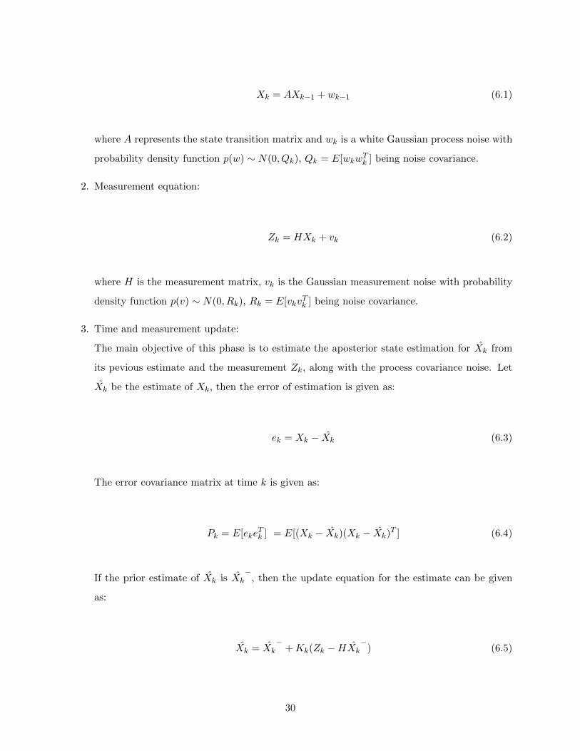
Xk = AXk−1 + wk−1 (6.1)
where A represents the state transition matrix and wk is a white Gaussian process noise with
probability density function p(w) ∼ N(0, Qk), Qk = E[wkwTk ] being noise covariance.
2. Measurement equation:
Zk = HXk + vk (6.2)
where H is the measurement matrix, vk is the Gaussian measurement noise with probability
density function p(v) ∼ N(0, Rk), Rk = E[vkvTk ] being noise covariance.
3. Time and measurement update:
The main objective of this phase is to estimate the aposterior state estimation for Xk from
its pevious estimate and the measurement Zk, along with the process covariance noise. Let
Xk be the estimate of Xk, then the error of estimation is given as:
ek = Xk − Xk (6.3)
The error covariance matrix at time k is given as:
Pk = E[ekeTk ] = E[(Xk − Xk)(Xk − Xk)
T ] (6.4)
If the prior estimate of Xk is Xk−
, then the update equation for the estimate can be given
as:
Xk = Xk−
+Kk(Zk −HXk−
) (6.5)
30

where Kk is the Kalman gain. The term (Zk−HXk−
) is a measurement residual. Substituting
equation 6.2 in equation 6.5
Xk = Xk−
+Kk(HXk + vk −HXk−
) (6.6)
Now from equation 6.4 and equation 6.6
Pk = E[((I −KkH)(Xk − Xk−
)−Kkvk)(I −KkH)(Xk − Xk−
)−Kkvk)T ] (6.7)
The term (Xk− Xk−
) in above equation, is the error of the prior estimate and is independent
of the measurement noise. Thus the expectation in 6.7 is given as:
Pk = (I −KkH)E[(Xk − Xk−
)(Xk − Xk−
)T ](I −KkH) +KkE[vkvTk ]KT
k
Pk = (I −KkH)P−k (I −KkH)T +KkRkK
Tk
(6.8)
where P−k is the prior estimate of Pk. Differentiating the trace of Pk in equation 6.8 with
respect to Kk, noting the fact that error covariance matrix is independent with the gain i.e.
dPkdKk
= 0 , the value of Kalman gain can be computed as:
Kk = P−k H
T (HP−k H
T +R)−1 (6.9)
Thus from equation 6.8 and equation 6.9 Pk can be simplified as:
Pk = (I −KkH)P−k (6.10)
31

6.1.2 Kalman Filter for Multi Target Tracking
A structure was defined to maintain the state of a tracked object. The parameters of the tracking
structure are:
• Tracking Index(ID): Tracking Index is used as the identity for each track and is used in data
association.
• Age of the track (AT): the number of frames since the track was first detected (Age of the
Track)
• Total Visible Count (TVC): number of frames in which tge track was actually detected.
• Kalman filter object (KF): for Kalman filter tracking
• bounding box (BB): to display the location of the track at the particular frame.
• state (State): parameter for initializing the Kalman filter object
• measurement (Meas): Kalman filter parameter update
• tracking points (TP): tracking point store the center point of the bounding box in each track
from the first frame until the track is completely lost.
• non visible count(NVC): to count the consecutive detection lost
For each detection in very first frame and also for new detections in other frames, the structure
assign a ID, initializes the KF, assign the detection bounding box information to the Kalman filter
State and Meas parameter and BB, initializes the AT and TVC to 1 and NVC to 0, stores the
centroid of bounding box in TP. In the successive frame if the same pedestrian is detected then
AT, and TVC are increased by 1, KF updates the State and Meas parameter. The bounding box
information was updated from the updated Meas variables, and the TP vector will again stores the
center of BB. For a failure detection, AT and NVC were increased by unity, KF estimates the new
State. BB and TP were updated from the new State only. A track will be deleted if NVC count
exceeds 4. This was also helpful in removing some noisy detection to stay for longer period of time
in the track. This tracking structure was very useful to handle new detections and also removing
the track when a particular pedestrian is out of the scene.
32
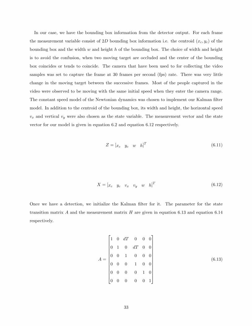
In our case, we have the bounding box information from the detector output. For each frame
the measurement variable consist of 2D bounding box information i.e. the centroid (xc, yc) of the
bounding box and the width w and height h of the bounding box. The choice of width and height
is to avoid the confusion, when two moving target are occluded and the center of the bounding
box coincides or tends to coincide. The camera that have been used to for collecting the video
samples was set to capture the frame at 30 frames per second (fps) rate. There was very little
change in the moving target between the successive frames. Most of the people captured in the
video were observed to be moving with the same initial speed when they enter the camera range.
The constant speed model of the Newtonian dynamics was chosen to implement our Kalman filter
model. In addition to the centroid of the bounding box, its width and height, the horizontal speed
vx and vertical vy were also chosen as the state variable. The measurement vector and the state
vector for our model is given in equation 6.2 and equation 6.12 respectively.
Z = [xc yc w h]T (6.11)
X = [xc yc vx vy w h]T (6.12)
Once we have a detection, we initialize the Kalman filter for it. The parameter for the state
transition matrix A and the measurement matrix H are given in equation 6.13 and equation 6.14
respectively.
A =
1 0 dT 0 0 0
0 1 0 dT 0 0
0 0 1 0 0 0
0 0 0 1 0 0
0 0 0 0 1 0
0 0 0 0 0 1
(6.13)
33

H =
1 0 0 0 0 0
0 1 0 0 0 0
0 0 0 0 1 0
0 0 0 0 0 1
(6.14)
The process covariance noise Q and measurement covariance noise R are given as in equation 6.15
and equation 6.16 respectively.
Q =
e−2 0 0 0 0 0
0 e−2 0 0 0 0
0 0 2.0 0 0 0
0 0 0 1.0 0 0
0 0 0 0 e−2 0
0 0 0 0 0 e−2
(6.15)
R =
e−1 0 0 0 0 0
0 e−1 0 0 0 0
0 0 0 0 e−1 0
0 0 0 0 0 e−1
(6.16)
where dT = 1fps . For each
6.2 Optical Flow
In an static camera video, the motion of the moving objects are represented by the relative shift
of the pixels in the consecutive frames. When the frame per rate is high, a pixel I(x, y) of certain
intensity or color in tth frame, will not not move too far in the (t + 1)th assuming that the color
or brightness constancy is maintained. This small motion of that particular pixel can be obtained
using optical flow.
34
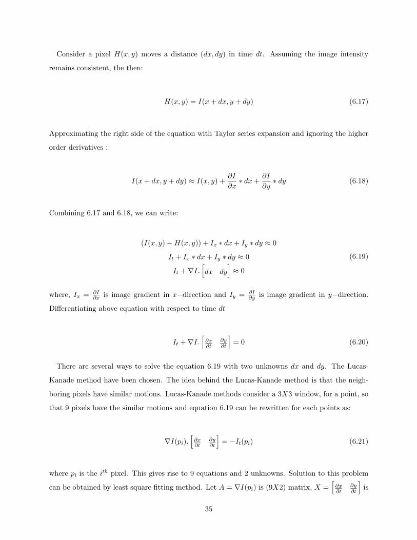
Consider a pixel H(x, y) moves a distance (dx, dy) in time dt. Assuming the image intensity
remains consistent, the then:
H(x, y) = I(x+ dx, y + dy) (6.17)
Approximating the right side of the equation with Taylor series expansion and ignoring the higher
order derivatives :
I(x+ dx, y + dy) ≈ I(x, y) +∂I
∂x∗ dx+
∂I
∂y∗ dy (6.18)
Combining 6.17 and 6.18, we can write:
(I(x, y)−H(x, y)) + Ix ∗ dx+ Iy ∗ dy ≈ 0
It + Ix ∗ dx+ Iy ∗ dy ≈ 0
It +∇I.[dx dy
]≈ 0
(6.19)
where, Ix = ∂I∂x is image gradient in x−direction and Iy = ∂I
∂y is image gradient in y−direction.
Differentiating above equation with respect to time dt
It +∇I.[∂x∂t
∂y∂t
]= 0 (6.20)
There are several ways to solve the equation 6.19 with two unknowns dx and dy. The Lucas-
Kanade method have been chosen. The idea behind the Lucas-Kanade method is that the neigh-
boring pixels have similar motions. Lucas-Kanade methods consider a 3X3 window, for a point, so
that 9 pixels have the similar motions and equation 6.19 can be rewritten for each points as:
∇I(pi).[∂x∂t
∂y∂t
]= −It(pi) (6.21)
where pi is the ith pixel. This gives rise to 9 equations and 2 unknowns. Solution to this problem
can be obtained by least square fitting method. Let A = ∇I(pi) is (9X2) matrix, X =[∂x∂t
∂y∂t
]is
35

(2X1) matrix and Y = −It(pi) is (9X1) matrix. Then inorder to solve the equation 6.21 ||AX−Y ||2
should be minimized, given that
AX = Y
ATAX = ATY
If ATA is invertible, with large eigen values, the above equation can give optimal solution. The
final equation can be written as:
∑ IxIx∑IxIy∑
IxIy∑IyIy
dxdy
=
IxItIyIt
(6.22)
Now the final equation have two equations and two unknowns and is solvable. Here the matrix
ATA is Harris corner detector matrix, indicating that corners are the good features for matching
or tracking.
6.2.1 Multi Target Tracking using Optical Flow
The tracking data structure for multi-target tracking using optical flow is almost similar to the
tracking data structure defined for Kalman filter tracking except the Kalman filter object, Kalman
filter state variable and Kalman filter measurement variable were replaced by a optical flow feature
vector (FV) to handle the new detections, updating the existing tracks and deleting the particular
track if they no longer appear in the camera view. The feature vector (FV) was initialized for each
new detection and was updated in every successive frames.
6.3 Data Association in Multi-Target Tracking
Detections are provided as the input to the tracking system. These detections initialize the
Kalman filter tracker in the system [27]. During the tracking process, the position of a detected
pedestrian will be predicted for the next frame. The predicted position was compared with the
actual detections from the detector. If the any of the detected measurement was found close to the
predicted measurement, that measurement was used to update our Kalman filter tracker for the
particular pedestrian.
36

In case of multi-target tracking problem, we need to resolve the data association problem.
Multiple detections from the detector need to be assigned to the multiple tracks. The greedy
matching algorithm was used to resolve this assignment problem. Each detection was compared
with all of the existing tracks using the Euclidean measure. Using just the centroid for distance
measure may results in wrong assignment if two people who are very closer but moving in opposite
direction. Instead of using the single point for computing the distance between the detection and
tracking, we used two points (centroid and the bottom right corner of the bounding box) from the
detection window and the previous track to compute the distance. A detection having minimum
distance with any of the existing track is more likely to be matched with the track. However, the
presence of noise and acquisition error in measurement a more reliable a decision rule for associating
the detections and track was set as given by equation 6.23.
d21 + d2
2 < 50 (6.23)
where d1 is distance between the centroid of track i from previous frame and detectionj from cur-
rent frame. d2 is distance between the bottom right corner of the track i from previous frame and
the bottom right corner of the detection j from current frame. This prevents a track from matching
too far away, which is likely to be separate object.
Data association in moving object detection using background subtraction and optical flow is
a bit more complicated because of inconsistencies in the bounding box across the detected objects
[24, 37]. The size of bounding boxes changes from the background subtraction method unlike in
Haar and LBP detector. So, the cost function for data association is defined as given in equation
6.24
f(D,A) = αD2ij + (1− α)|At,i −Ad,j | (6.24)
where α = 0.75, Dij is distance between the centroid of track i from previous frame and detection j
from current frame, At,i is area of track i from previous frame and Ad,j is the area of jth detection
from current frame. f(D,A) < 150 is assumed to be a match. In order word, smaller the cost
37

function, the two objects are more likely to have correspondence. A low value of α is chosen to
give high weight to the distance metrics than the change in area metrics.
38

Chapter 7
Activity Analysis
Detection and tracking results can be very useful in understanding the underlying behavior. In
this chapter we will discuss two application are of the detection result. In the first section we will
discuss video stabilization, in a scene where the video frames are captured from the camera from
UAS. The video stabilization gives the easy view for the observer to focus on the target of interest
when the video frames are shaky. In the second section we will highlight the pedestrian behavior
in the scene.
7.1 Video Stabilization
Camera mounted on the high altitude towers can be affected by the strong wind causing the
captured video frame to be shaky. While hardware solutions, including dampened mounting and
high quality gimbals, are effective to remove such unwanted motions, still the camera motions due
to panning and zooming exists. The UAS motion also brings a large amount of jittering in the
captured video sequence. Video stabilization is the art of removing such motions between frames.
Some of the software techniques developed so far will compensate the motion in the whole frame
or compensate motion based on object.
7.1.1 Object Centric Video Stabilization
Often times there comes the situation where the location of particular object of interest will be
the focus area in the surveillance system. Object centric stabilization makes it easy for the human
observer to focus on the object of interest itself and away from the distracting camera movements.
The UAS will move in an attempt to keep that object of interest in the field of view. The raw video
39

collected will not be smooth because of the camera motion. The video can be smoothed about
object using the object detection framework.
The particular object of interest was detected in the first frame. The same object detected in
the rest of the frames was warped and smoothed to maintain the same view and same location
as seen in the first frame making the less important background move quickly around. Thus, an
object centric video stabilization is established, which will make the monitoring task easier, and
helps in activity analysis. Following steps have been followed for object centric video stabilization:
• Object detector provides the bounding box location of the detected object. Only a single
object is selected for stabilization. Let the bounding rectangle for this object be R1.
• The bounding box location for the same same object in next frame frame is extracted from
the detector. Let the bounding rectangle for second frame be R2.
• Affine transform between R1 and R2 was computed and applied over the second frame.
• For nth frame Affine transform between the R1 and Rn was computed and applied over that
frame.
• To make the stabilized video smooth the affine transform matrix obtained for nth is computed
as the weighted average of all the affine transform matrices obtained for past frames. If An is
the affine transform matrix obtained between bounding rectangle R1 and Rn, for smoothing
the video, An is replaced by:
An =1
2An +
1
2An−1 (7.1)
Let (x1,1, y1,1), (x1,2, y1,2), and (x1,3, y1,3) be the top left, top right and bottom right corners of
the bounding box of the detected object in first frame. The goal of the affine transform is to find
a suitable transformation matrix M which can map the same three points on the bounding box
given by (xn,1, yn,1), (xn,2, yn,2), and (xn,3, yn,3) respectively from nth frame. Then affine transform
between these set of points is given by the equation 7.2
40

x1,1 x1,2 x1,3
y1,1 y1,2 y1,3
1 1 1
︸ ︷︷ ︸
X1
=
a b tx
c d ty
0 0 1
︸ ︷︷ ︸
An
xn,1 xn,2 xn,3
yn,1 yn,2 yn,3
1 1 1
︸ ︷︷ ︸
Xn
(7.2)
where a and d gives scaling in x− axis and y − axis respectively, and b and c gives x− axis and
y − axis shearing respectively. The term t = (tx, ty) are the translation parameters to shifts the
origin to point (tx, ty). Equation 7.2 has 6 equations and 6 unknown parameter of the matrix An,
which can be easily solved if An is invertible.
The video stabilization technique discussed above was implemented on the UCF Balloon dataset
[38]. In this video, a camera is mounted on a balloon and is monitoring a parked car. The result
of object centric stabilization is shown in the Figure 7.1.
The raw frame from the video is shown in the left image, the affine transformed image of the
particular frame on view is is shown in the middle image and the frame after smoothing is shown
at the right. The blue bounding box, drawn on same location on all three images, is the position
of the car in the first frame. The green bounding box shows the current bounding box for the car.
Notice there is a large amount of camera motion in this video as the car has moved in all directions
away from the initial position (in blue). The camera motion is so abrupt that the image moves
in different positions in the successive frames. The video stabilization brings the car back to its
original position as seen in first frame and provides a smooth playback.
7.2 Usuage of Heatmap
Detections and tracking results are utilized with the kernel density estimation to highlight the
most probable routes [39]. The Figure 7.3 7.2 clearly shows that the people mostly use the walkways
to reach their destinations. Even within the walkway there are preferred paths such as straight
way from exit of the building to the parking garage. Small portion of the walkway is utilized by
pedestrian.
The heat maps from the ground truth (obtained from the first 33 seconds of the video only)
shows a thin line used by the pedestrian, However the heat map for Haar LBP and the combined
41

(a)
(b)
Figure 7.1: Video stabilization at two different frames. The first images in both (a) and (b) showthe actual frame obtained from the UAS. These images shows that the car is located at the randomlocation in the field of view. The blue bounding box, as shown in all frames, is position of the carin first frame and green bounding box is the detection of car in current frame. The object-centricstabilization goal is to maintain the position of the car in the blue bounding box during trackingas shown in the second image. The third image provides the smoothed version for pleasing videoplayback.
detector was obtained for the same frame using 30 different thresholds. Both Haar and LBP detector
seems to be confused more by the vertical lines, trees, LBP detector shows more continuous path,
indicating its high detection rate. The combined Haar and LBP detector was reduce the false
positive. Our result shows that Haar did a fairly good job than any other detectors in detecting
one of the two occluded pedestrian at the bottom right corner of the image. Combining the track
over Haar and LBP detector accurately maps the detector along the main walking area, but on
the other hand also increased the false detections too. GMM shows that the most likely area of
pedestrians occurrence to be almost equally probable than any other detectors.
42

(a) Overlay Heatmap-Ground Truth (b) Probability Density-Ground Truth
(c) Overlay Heatmap-Haar (d) Probability Density-Haar
(e) Overlay Heatmap-LBP (f) Probability Density-LBP
Figure 7.2: Learning usage routes based of detection and tracking data. The ground truth Figurea, b clearly show tight usage patterns. Due to errors is detection and tracking, the heatmapsgenerated using LBP and Haar are not as crisp, but still represent the scene well. Notice that inboth LBP and Haar, the false detections on a tree results in a high probability location.
43

(a) Overlay Heatmap-Haar+LBP (b) Probability Density-Haar+LBP
(c) Overlay Heatmap-Haar+LBP+Track (d) Probability Density-Haar+LBP+Track
(e) Overlay heatmap-Motion (f) Probability Density-Motion
Figure 7.3: Learning usage routes based of detection and tracking data. Figure 7.3a shows lessdetections and 7.3a shows added false detections. f shows that certain parts are almost equallyprobable to have pedestrians.
44

Chapter 8
Edge Neural Network for False
Rejection
The accuracy of the detector can be improved if false detections can be reduced. The pedestrian
detectors that were evaluated were occasionally confused with a lamp post, trees and the concrete
spacing lines in the walkway. In other words, the most common confusion was still with the shape
of the objects in the search window. The performance of the detector can be improved if those
frequent confusions can be addressed. In order to address the confusion, a two-layer error back
propagation neural network has been implemented as shown in Figure 8.1. The network was de-
signed with 805 edge features in the form of 1’s and −1 as inputs, 20 nodes in hidden layer and 2
output nodes. Input to this neural network was the canny edge information from each detection.
The neural network classifies as either a true or false detection based on edge information.
A cropped image is obtained from the original image with a detection bounding box to begin
processing. The canny edge detector was applied to each sub-image and the resulting edge image
is used as input the neural network for training. Each detection was compared with ground truth
information using the 50% overlap criteria to determine if the training example would be a positive
or negative example for training. The details for the false detection rejection system is summarized
in algorithm 8.1.
The edge information and label was input to the neural network for training over the first 800
frames using the LBP detector. The final 200 frames were used for testing. The learning curve in
45
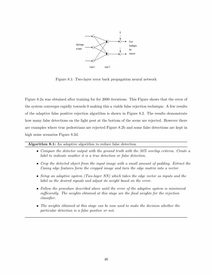
Figure 8.1: Two-layer error back propagation neural network
Figure 8.2a was obtained after training for for 2000 iterations. This Figure shows that the error of
the system converges rapidly towards 0 making this a viable false rejection technique. A few results
of the adaptive false positive rejection algorithm is shown in Figure 8.2. The results demonstrate
how many false detections on the light post at the bottom of the scene are rejected. However there
are examples where true pedestrians are rejected Figure 8.2b and some false detections are kept in
high noise scenarios Figure 8.2d.
Algorithm 8.1: An adaptive algorithm to reduce false detection
• Compare the detector output with the ground truth with the 50% overlap criteria. Create alabel to indicate weather it is a true detection or false detection.
• Crop the detected object from the input image with a small amount of padding. Extract theCanny edge features form the cropped image and turn the edge matrix into a vector.
• Setup an adaptive system (Two-layer NN) which takes the edge vector as inputs and thelabel as the desired signals and adjust its weight based on the error.
• Follow the procedure described above until the error of the adaptive system is minimizedsufficiently. The weights obtained at this stage are the final weights for the rejectionclassifier.
• The weights obtained at this stage can be now used to make the decision whether theparticular detection is a false positive or not.
46

(a) Neural Network Learning Curve (b) Perfect False Rejection
(c) Missed Detection (d) Incomplete Rejection in Noise
Figure 8.2: Result of adaptive algorithm for false positive rejection. With false positive rejection,the system is more robust to the commonly occurring false detections. (a) The learning curveshows how the adaptive system converges to learn optimal classifier weights. (b) Both pedestriansare correctly detected and all the false detections on the post and walkway are perfectly rejected.(c) One of the true detections is missed. (d) Noisy image with improved performance but still twofalse detections (one on the tree).
47

Chapter 9
Results and Discussion
In this section an evaluation of different color-based pedestrian detection algorithms are compared
on the UNLV Thermal-Color Pedestrian Dataset. The evaluation compares the detection accuracy
and false detections and computational efficiency. Kalman filter and Optical flow tracking were
compared based on their speed, and number of tracks. Images of the detection and tracking results
are also shown in this chapter.
9.1 Performance Metrics and ROC Curve
In order to evaluate the performance of the detection and tracking system, 1011 frames from
UNLV Color Thermal dataset was manually annotated. The detector (Haar or LBP) performance
at a particular operating point (i.e. a specific detection threshold) is evaluated using the following
measures:
1. True Positive Detection: For each detection bounding box, if there exist a matching bounding
box in the ground truth, then the corresponding detection is treated as a true positive. A
bounding box match requires an overlap greater than or equal to 50% Equation (5.9).
2. False Positive Detection: For all detections in a frame, if there exists some bounding boxes
that do not have any corresponding bounding box in the ground truth with area of overlap
≥ 50%, then those detections are treated as false positives.
3. False Negative: Any ground truth pedestrian having no corresponding bounding box from the
detector with the 50% overlap rule is a false negative. This is also called a missed detection.
48

4. True Positive Rate (TPR): It is the ratio of total number of True Positives detected in the
entire dataset and the total number positives from the ground truth.
5. False Positives Per Frame (FPPF): Ratio of total number of false positives and the number of
frames. This is used instead of the more traditional false positive rate (FPR) since it better
reflects performance for video.
6. False Negatives Per Frame (FNPF): Total number of missed detections divided by total
number of frames.
A strong system should have TPR close to 1 and FPPF and FNPF close to 0. This would
indicate that in each frame only the true pedestrians were detected without any mistakes. A more
detailed comparison of performance over various detector settings can be viewed in a graph form
using the receiver operating characteristics (ROC) curve. The curve is generated by plotting TPR
against FPR. However for the detection and the tracking system in video, the curve is generated
by plotting TPR against FPPF. The ROC curves gives the visual overview of each detector over
different thresholds. A good detector will have the curve rising rapidly towards the upper left
corner which indicates better performance over a wider range of operational settings. The system
threshold condition for the desired outcome (fixed FPPF or desired TPR) can be obtained from
the curve for a fair comparison between detectors.
9.2 Performance Evaluation for Detectors on UNLV dataset
The performance of the whole detection and the tracking system was evaluated on the annotated
UNLV Thermal dataset using gray channel. The performance results are shown in table 9.1 (Note:
these give the results at highest TPR). The Table 9.1 shows that the both the Haar and the LBP
detector are almost detecting an equal number of pedestrians correctly, however the false detection
per frame in the Haar detector is higher than in comparison to the LBP detector. The third detector
(HAAR+LBP), which combines the detection of Haar and LBP with the 50% overlap rule, is able
to reduce the false positive per frame slightly, but it comes at the cost of reduced TPR, because
some of the detections found by Haar will be missed by the LBP detector or vice versa. When
the detector was combined with tracking, performance of the system increases dramatically. The
detector accuracy on Haar+LBP on green channel almost increased by 20% with a significant drop
in false detection in FPPF and missed detections per frame. The motion based detection works
49

very well for the UNLV Thermal data since the camera is in a fixed position. The detector almost
matches the best TPR of Haar+LBP with tracking and has the lowest FPPF.
Some examples of our detection result is shown in Figure 9.1. The top row shows the appearance-
based detectors (Haar, LBP, Haar+LBP) while the next two rows show the background subtraction
results. Notice the appearance-based detectors are not able to detect pedestrians that are cut-off at
the edge of the image frame and can be confused by the tall skinny light post in the bottom middle
of the frame. The background subtraction motion detector does a good job of finding moving
pedestrians. However, it is sensitive so some pedestrians are not well segmented and compression
artifacts result in false detections.
Table 9.1: Pedestrian detection and tracking performance
Detector TPR FPPF FNPF
HAAR 0.4818 9.5143 2.6459LBP 0.4845 6.7616 2.6291
HAAR+LBP 0.4211 2.8961 2.9407KALMAN+HAAR+LBP 0.6803 1.0524 1.6291
GMM 0.6798 0.8683 1.6447
The corresponding ROC curves to further characterize the performance of the detection and
the tracking system is shown in Figure 9.2. The plot clearly shows that the LBP detector has
better performance in comparison to Haar detector.The Haar detector has the highest total FPPF
of all detectors. The combined Haar+LBP detector lowers the FPPF and slightly bumps up the
performance over just Haar. By adding tracking over this fused detector, the TPR increases greatly
up to a maximum of 0.68 which is the highest of all the compared detection schemes. This highlights
how incorporating the tracking system increases the confidence in the detection of true objects in
the scene. The GMM-based background subtraction motion detector has a similarly high TPR
but the lowest FPPF rates. This classifier does much better than any of the other detectors but is
applicable for stationary cameras which limits its flexibility for other scenarios like UAS surveillance.
50

(a) (b) (c)
(d)
(e)
Figure 9.1: Detection result. Detection from Haar, LBP, combined Haar and LBP, and GMM.(a), (b), (c) shows the Haar, LBP and combined detector in green, red and blue bounding box.Some of the true pedestrians are missed when they are not fully in the video frame while somenon-pedestrian regions are mistakes (such as the light post). (d), (e) show the detection resultsfrom the background subtraction method. The first image provides the background image whichslowly evolves in time. The second image is the extracted foreground regions while the third imagehas the detected objects outlined in green bounding boxes. Some noise detections can be observedin (e) from compression artifacts.
51

Figure 9.2: ROC of pedestrian detectors. ROC to show the performance of pedestrian detection.It shows that LBP has better performance over the Haar detector. The Haar -LBP detectorreduces the FPPF to less than 3, and incorporating the tracking system with combined detectordramatically raises the system performance. The GMM-based motion detection system has thebest results of all in the static camera scenario.
9.3 Performance Evaluation for Trackers on UNLV dataset
In order to compare the performance of the tracking system, we consider the number of times
a particular pedestrian is actually detected, known as the total visible count (TVC), how long the
track exist i.e. age of the track (Age), and the execution time for tracking during 1010 frames.
Table 9.2 shows the time of execution, both age and the TVC greater than 50 and 100 and Table
9.3 shows the top 5 tracks that exist for a longer period of time for detailed comparison. Examples
of the tracknig results can be found in Figure 9.3.
Table 9.2: Comparing tracking methods based on the total visible count and age of the track
Tracking Total Tracks Time (Sec) TVC > 50 Age > 50 TVC > 100 Age > 100
Kalman Filter(Haar+LBP) 128 204.901 13 22 7 12Kalman Filter(LBP) 145 82.5995 57 53 35 42
Optical Flow 27 121.844 6 7 4 4
As shown in Table 9.2, the Kalman filter based tracking with LBP detector is faster than any
52
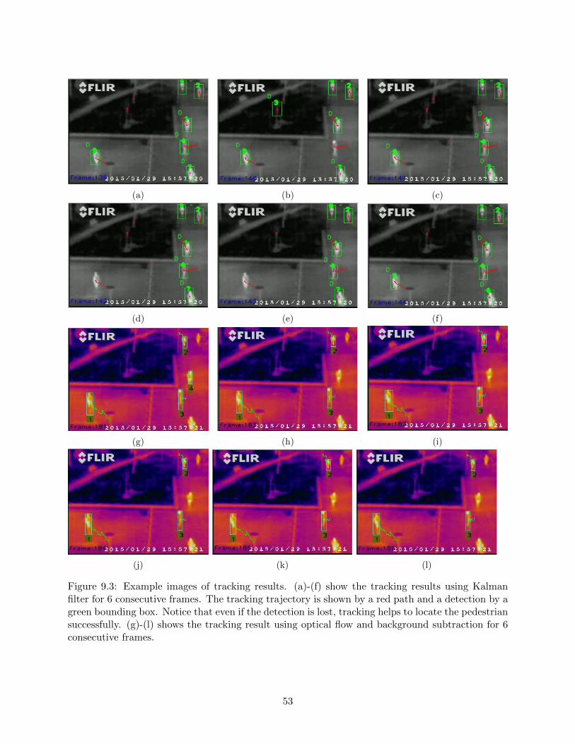
(a) (b) (c)
(d) (e) (f)
(g) (h) (i)
(j) (k) (l)
Figure 9.3: Example images of tracking results. (a)-(f) show the tracking results using Kalmanfilter for 6 consecutive frames. The tracking trajectory is shown by a red path and a detection by agreen bounding box. Notice that even if the detection is lost, tracking helps to locate the pedestriansuccessfully. (g)-(l) shows the tracking result using optical flow and background subtraction for 6consecutive frames.
53
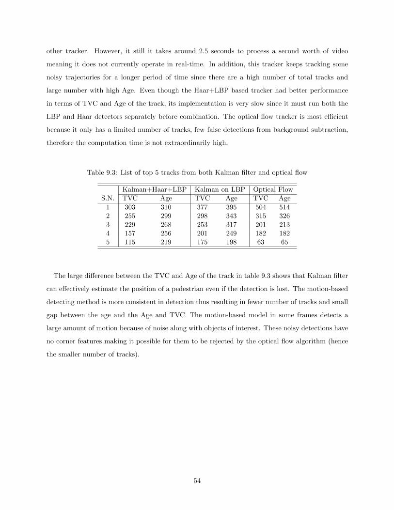
other tracker. However, it still it takes around 2.5 seconds to process a second worth of video
meaning it does not currently operate in real-time. In addition, this tracker keeps tracking some
noisy trajectories for a longer period of time since there are a high number of total tracks and
large number with high Age. Even though the Haar+LBP based tracker had better performance
in terms of TVC and Age of the track, its implementation is very slow since it must run both the
LBP and Haar detectors separately before combination. The optical flow tracker is most efficient
because it only has a limited number of tracks, few false detections from background subtraction,
therefore the computation time is not extraordinarily high.
Table 9.3: List of top 5 tracks from both Kalman filter and optical flow
S.N.Kalman+Haar+LBP Kalman on LBP Optical FlowTVC Age TVC Age TVC Age
1 303 310 377 395 504 5142 255 299 298 343 315 3263 229 268 253 317 201 2134 157 256 201 249 182 1825 115 219 175 198 63 65
The large difference between the TVC and Age of the track in table 9.3 shows that Kalman filter
can effectively estimate the position of a pedestrian even if the detection is lost. The motion-based
detecting method is more consistent in detection thus resulting in fewer number of tracks and small
gap between the age and the Age and TVC. The motion-based model in some frames detects a
large amount of motion because of noise along with objects of interest. These noisy detections have
no corner features making it possible for them to be rejected by the optical flow algorithm (hence
the smaller number of tracks).
54

Chapter 10
Conclusion and Future Work
10.1 Summary of Works
In this report, we collected the UNLV Color Thermal Pedestrian Dataset to provide a surveillance-
level view of pedestrians for different computer vision algorithm. Approximately 1000 frames of
thermal video was manually annotated for benchmarking of thermal detection techniques.
We implemented different boosted cascade pedestrian detectors using Haar features, texture
based LBP, and a Haar-LBP combination along with motion detection with background detection.
The detection evaluation result of detection show the LBP is most effective at reducing false positive
than Haar while the combination of Haar-LBP significantly lowered the FPR but at a cost of lower
TRP. Incorporating Kalman tracking on top of Haar and LBP not only increases the TPR but also
provides a more pleasing continuous activity heatmap However, tracking did increase the FPR.
Results show that the background subtraction-based detection had higher TRP at low FPR than
Haar, LBP, their combination along with Kalman filter. Haar and LBP detectors, trained with
limited training samples and tested on the entirely different dataset, were occasionally confused
with the shape of the lamp post and the trunk of tree (the shape being almost similar to that
of a pedestrian when looked through a window) giving a large false detection. Thus, it can be
concluded that motion based detectors have better performance than poorly trained appearance
based detectors in thermal images when the camera used is static in nature and target are moving.
However, in case of detecting the stationery targets, combination of Haar, LBP and Kalman filter
will outperform background subtraction based detectors.
55

An evaluation of tracking techniques examined Kalman filter over detections from LBP and
combined Haar+LBP and optical flow for motion detection. Results demonstrated that objects
were easily tracked using a simple motion model or using features. Kalman filter was shown to
have faster execution time over optical flow but would track false positives for a longer time period.
The Kalman filter was better able to predict a pedestrian position even if the detection was lost
for a longer period of time. Optical flow was found to be better at rejecting noisy detections which
tended not to have important corner features to track.
Finally we demonstrated a method to identify and visualize pedestrian behavior and describe
a surveillance scene using detection and tracking results. We demonstrate that the usage routes
of pedestrians are small with respect to space. An adaptive learning algorithm was developed to
correct and reject false detections and improve detector performance.
10.2 Future Work
Video surveillance in multispectral images is a growing and an important topic for future research.
Some suggestions to improve the surveillance system based on our results are described below:
• Since there are not many publicly available datasets for aerial multispectral images, the first
recommendation is to collect more thermal imagery datasets. It would be best to collect this
in synchronization with visible spectrum cameras of the same scene for comparison purposes.
• In order to improve the performance of the Haar and LBP detector, the detector should be
trained with a larger number of positive samples and using non-pedestrian thermal images
for negative samples.
• The Kalman filter can be used to predict the position of a pedestrian in a future frame. When
the detector fails, the prediction can be used re-check (with more complex classifier) an area
when there is a miss and no match of a track to ensure fewer missed detections.
• Develop elegant methods to combine motion and appearance detection techniques to have
the benefits of both.
• Integrate thermal images with the visible light images for detection and tracking fusion.
• More complex techniques such as deformable parts model (DPM) for detection and particle
filters for tracking should be examined since the DPM better handles object deformations
56

and particle filtering is independent of a motion model and can handle fast motions that may
be encountered in UAS operation from zooms and gimbals.
57

Bibliography
[1] “Closed-circuit television— wikipedia, the free encyclopedia,” [Online; accessed 24-September-
2015]. [Online]. Available: http://en.wikipedia.org/w/index.php?title=Moose Jaw&oldid=
16357282
[2] K. J. Havens and E. J. Sharp, “Using thermal imagery in the aerial survey of animals,” vol. 26,
no. 1, pp. ”17–23, Spring, 1998.
[3] N. Dalal and B. Triggs, “Histograms of oriented gradients for human detection,” in Computer
Vision and Pattern Recognition, 2005. CVPR 2005. IEEE Computer Society Conference on,
vol. 1, June 2005, pp. 886–893 vol. 1.
[4] P. Viola and M. Jones, “Robust real-time face detection,” in Computer Vision, 2001. ICCV
2001. Proceedings. Eighth IEEE International Conference on, vol. 2, 2001, pp. 747–747.
[5] ——, “Rapid object detection using a boosted cascade of simple features,” in Computer Vision
and Pattern Recognition, 2001. CVPR 2001. Proceedings of the 2001 IEEE Computer Society
Conference on, vol. 1, 2001, pp. I–511–I–518 vol.1.
[6] P. Felzenszwalb, R. Girshick, D. McAllester, and D. Ramanan, “Object detection with dis-
criminatively trained part-based models,” Pattern Analysis and Machine Intelligence, IEEE
Transactions on, vol. 32, no. 9, pp. 1627–1645, Sept 2010.
[7] S.-K. Pavani, D. Delgado, and A. F. Frangi, “Haar-like features with optimally weighted
rectangles for rapid object detection,” Pattern Recogn., vol. 43, no. 1, pp. 160–172, Jan. 2010.
[Online]. Available: http://dx.doi.org/10.1016/j.patcog.2009.05.011
[8] “Local binary patterns histograms.” [Online]. Available: http://docs.opencv.org/modules/
contrib/doc/facerec/facerec tutorial.html#local-binary-patterns-histograms
[9] T. Ahonen, A. Hadid, and M. Pietikainen, “Face description with local binary patterns: Ap-
plication to face recognition,” Pattern Analysis and Machine Intelligence, IEEE Transactions
on, vol. 28, no. 12, pp. 2037–2041, Dec 2006.
[10] P. Dollar, Z. Tu, P. Perona, and S. Belongie, “Integral channel features,” in BMVC, 2009.
[11] A. Gszczak, T. P.Breckon, and J. Han, “Real-time people and vehicle detection from uav
imagery,” in Proceeding of SPIE : Intelligent Robots and Computer Vision XXVIII : Algorithms
and Techniques, San Francisco, California, Jan.
58

[12] J. van Gemert, C. Verschoor, P. Mettes, K. Epema, L. Koh, and S. Wich, “Nature conservation
drones for automatic localization and counting of animals,” in Computer Vision - ECCV 2014
Workshops. Springer International Publishing, 2015, pp. 255–270.
[13] S. Hwang, J. Park, N. Kim, Y. Choi, and I. So Kweon, “Multispectral pedestrian detection:
Benchmark dataset and baseline,” in The IEEE Conference on Computer Vision and Pattern
Recognition (CVPR), June 2015.
[14] M. Teutsch, T. Mueller, M. Huber, and J. Beyerer, “Low resolution person detection with a
moving thermal infrared camera by hot spot classification,” in Computer Vision and Pattern
Recognition Workshops (CVPRW), 2014 IEEE Conference on, June 2014, pp. 209–216.
[15] A. C. J. H. P. R. B. Sirmacek, M. Wegmann and S. Decha, “Automatic population counts
for improved wildlife management using aerial photography,” in International Congress on
Environmental Modelling and Software, 2012.
[16] C. Stauffer and W. Grimson, “Adaptive background mixture models for real-time tracking,”
in Computer Vision and Pattern Recognition, 1999. IEEE Computer Society Conference on.,
vol. 2, 1999, p. 252 Vol. 2.
[17] T. Pollard and M. Antone, “Detecting and tracking all moving objects in wide-area aerial
video,” in Computer Vision and Pattern Recognition Workshops (CVPRW), 2012 IEEE Com-
puter Society Conference on, June 2012, pp. 15–22.
[18] J. Xiao, H. Cheng, H. Sawhney, and F. Han, “Vehicle detection and tracking in wide field-of-
view aerial video,” in Computer Vision and Pattern Recognition (CVPR), 2010 IEEE Confer-
ence on, June 2010, pp. 679–684.
[19] V. Reilly, H. Idrees, and M. Shah, “Detection and tracking of large number of targets in wide
area surveillance,” in Computer Vision ECCV 2010, ser. Lecture Notes in Computer Science,
K. Daniilidis, P. Maragos, and N. Paragios, Eds. Springer Berlin Heidelberg, 2010, vol. 6313,
pp. 186–199.
[20] J. Prokaj and G. Medioni, “Persistent tracking for wide area aerial surveillance,” in Computer
Vision and Pattern Recognition (CVPR), 2014 IEEE Conference on, June 2014, pp. 1186–
1193.
[21] J. Zhu, O. Javed, J. Liu, Q. Yu, H. Cheng, and H. Sawhney, “Pedestrian detection in low-
resolution imagery by learning multi-scale intrinsic motion structures (mims),” in Computer
Vision and Pattern Recognition (CVPR), 2014 IEEE Conference on, June 2014, pp. 3510–
3517.
[22] M. S. Shirazi and B. Morris, “Contextual combination of appearance and motion for inter-
section videos with vehicles and pedestrians,” in 10th International Symposium on Visual
Computing, ISVC 2014, 2014, pp. 708–717.
[23] S. Baker and I. Matthews, “Lucas-kanade 20 years on: A unifying framework,”
Int. J. Comput. Vision, vol. 56, no. 3, pp. 221–255, Feb. 2004. [Online]. Available:
http://dx.doi.org/10.1023/B:VISI.0000011205.11775.fd
59

[24] M. S. Shirazi and B. Morris, “Vision-based vehicle queue analysis at junctions,” in Advanced
Video and Signal Based Surveillance (AVSS), 2015 12th IEEE International Conference on,
Aug 2015, pp. 1–6.
[25] J. G. Allen, R. Y. D. Xu, and J. S. Jin, “Object tracking using camshift
algorithm and multiple quantized feature spaces,” in Proceedings of the Pan-Sydney
Area Workshop on Visual Information Processing, ser. VIP ’05. Darlinghurst, Australia,
Australia: Australian Computer Society, Inc., 2004, pp. 3–7. [Online]. Available:
http://dl.acm.org/citation.cfm?id=1082121.1082122
[26] X. Li, K. Wang, W. Wang, and Y. Li, “A multiple object tracking method using kalman filter,”
in Information and Automation (ICIA), 2010 IEEE International Conference on, June 2010,
pp. 1862–1866.
[27] M. Shirazi and B. Morris, “Vision-based turning movement counting at intersections by co-
operating zone and trajectory comparison modules,” in Intelligent Transportation Systems
(ITSC), 2014 IEEE 17th International Conference on, Oct 2014, pp. 3100–3105.
[28] F. Xu, X. Liu, and K. Fujimura, “Pedestrian detection and tracking with night vision,” Intel-
ligent Transportation Systems, IEEE Transactions on, vol. 6, no. 1, pp. 63–71, March 2005.
[29] M. Arulampalam, S. Maskell, N. Gordon, and T. Clapp, “A tutorial on particle filters for
online nonlinear/non-gaussian bayesian tracking,” pp. 174–188, Feb 2002.
[30] A. Leykin and R. Hammoud, “Robust multi-pedestrian tracking in thermal-visible surveil-
lance videos,” in Computer Vision and Pattern Recognition Workshop, 2006. CVPRW ’06.
Conference on, June 2006, pp. 136–136.
[31] “Object tracking and classification beyond visual spectrum benchmark dataset collection,”
[Online; accessed 24-September-2015]. [Online]. Available: http://vcipl-okstate.org/pbvs/
bench/
[32] J. Davis and M. Keck, “A two-stage template approach to person detection in thermal im-
agery,” in Application of Computer Vision, 2005. WACV/MOTIONS ’05 Volume 1. Seventh
IEEE Workshops on, vol. 1, Jan 2005, pp. 364–369.
[33] J. W. Davis and V. Sharma, “Background-subtraction using contour-based fusion of thermal
and visible imagery,” Comput. Vis. Image Underst., vol. 106, no. 2-3, pp. 162–182, May 2007.
[Online]. Available: http://dx.doi.org/10.1016/j.cviu.2006.06.010
[34] H. A. . P. M. Ahonen T, “Face recognition with local binary patterns,” in Computer Vision,
ECCV 2004 Proceedings, Lecture Notes in Computer Science 3021, 2004, pp. 469–481.
[35] Z. Zivkovic, “Improved adaptive gaussian mixture model for background subtraction,” in Pat-
tern Recognition, 2004. ICPR 2004. Proceedings of the 17th International Conference on, vol. 2,
Aug 2004, pp. 28–31 Vol.2.
[36] A. Yilmaz, O. Javed, and M. Shah, “Object tracking: A survey,” ACM Comput. Surv.,
vol. 38, no. 4, Dec. 2006. [Online]. Available: http://doi.acm.org/10.1145/1177352.1177355
60

[37] M. S. Shirazi and B. Morris, “A typical video-based framework for counting, behavior and
safety analysis at intersections,” in Intelligent Vehicles Symposium (IV), 2015 IEEE, June
2015, pp. 1264–1269.
[38] “Ucf aerial action data set,” [Online; accessed 24-September-2015]. [Online]. Available:
http://crcv.ucf.edu/data/aerial/datacollect3/actions1.mpg2
[39] M. Shirazi and B. Morris, “Observing behaviors at intersections: A review of recent studies and
developments,” in Intelligent Vehicles Symposium (IV), 2015 IEEE, June 2015, pp. 1258–1263.
61

Curriculum Vitae
Graduate College
University of Nevada, Las Vegas
Santosh Bhusal
Degrees:
Bachelor’s of Degree in Electronics and Communication Engineering 2011
Tribhuvan University
Western Region Campus, Nepal
Thesis Title: Object Detection and Tracking in Wide Area Surveillance using Thermal Imagery
Thesis Examination Committee:
Chairperson, Dr.Brendan Morris, Ph.D.
Committee Member, Dr. Shahram Latifi, Ph.D.
Committee Member, Dr. Ebrahim Saberinia, Ph.D.
Graduate Faculty Representative, Dr. Alex Paz, Ph.D.
62