motion detection, object classiﬁcation and tracking for...

Motion Detection, Object Classification

and Tracking for

Visual Surveillance Application

Deepak Kumar Panda

Department of Electronics and Communication EngineeringNational Institute of Technology RourkelaRourkela-769 008, Odisha, India

Motion Detection, Object Classificationand Tracking for

Visual Surveillance Application

Thesis submitted in partial fulfillment

of the requirements for the degree of

Master of Technology

in

Communication and Signal Processing

by

Deepak Kumar Panda

(Roll: 210EC4316)

under the guidance of

Prof. Sukadev Meher

Department of Electronics and Communiation EngineeringNational Institute of Technology Rourkela

Rourkela-769 008, Odisha, India

Department of Electronics and Communication Engg.

National Institute of Technology Rourkela

Rourkela-769 008, Odisha, India.

June 6, 2012

Certificate

This is to certify that the thesis titled Motion Detection, Object Classifica-

tion and Tracking for Visual Surveillance Application by Deepak Kumar

Panda is a record of an original research work carried out under my supervision

and guidance in partial fulfillment of the requirements for the award of the degree of

Master of Technology degree in Electronics and Communication Engineering

with specialization in Communication and Signal Processing during the session

2011-2012.

Sukadev Meher

Professor

Acknowledgement

“The will of God will never take you where Grace of God will not protect you.”

Thank you God for showing me the path. . .

I owe deep gratitude to the ones who have contributed greatly in completion of this

thesis.

Foremost, I would like to express my sincere gratitude to my advisor, Prof. Sukadev

Meher for providing me with a platform to work on challenging areas of Motion

detection, object classification and tracking for visual surveillance application. His

profound insights and attention to details have been true inspirations to my research.

I am very much indebted to Prof. Sarat Kumar Patra, Prof. Banshidhar Majhi

and Prof. Kamala Kanta Mahapatra for providing insightful comments at different

stages of thesis that were indeed thought provoking.

My special thanks go to Prof. Ajit Kumar Sahoo, Prof. Upendra Kumar Sahoo

and Prof. Pankaj Kumar Sa for contributing towards enhancing the quality of the

work in shaping this thesis.

I would like to thank all my friends and lab–mates for their encouragement and

understanding. Their help can never be penned with words.

Most importantly, none of this would have been possible without the love and

patience of my family. My family to whom this dissertation is dedicated to, has been

a constant source of love, concern, support and strength all these years. I would like

to express my heartfelt gratitude to them.

Deepak Kumar Panda

Abstract

Visual surveillance in dynamic scenes, especially for humans and vehicles, is one

of the current challenging research topics in computer vision. It is a key technol-

ogy to fight against terrorism, crime, public safety and for efficient management of

traffic. The work involves designing of efficient visual surveillance system in complex

environments. In video surveillance, detection of moving objects from a video is im-

portant for object classification, target tracking, activity recognition, and behavior

understanding. Detection of moving objects in video streams is the first relevant step

of information and background subtraction is a very popular approach for foreground

segmentation. In this thesis, we have simulated different background subtraction

methods to overcome the problem of illumination variation, background clutter, shad-

ows, and camouflage. Object classification is done using silhouette template based

classification to categorize objects into human, group of human and vehicle. Detecting

and tracking of human body parts is important in understanding human activities.

We have proposed two methods to overcome the problem of object tracking in varying

illumination condition and background clutter. For target tracking of interested ob-

ject in the consecutive video frames, we have used normalized correlation coefficient

(NCC). NCC is robust to varying illumination condition. Template is updated on

every frame to minimize the template drift problem and it also tries to cope with

short-lived occlusion and background clutter. In order to extend the surveillance

area and overcome occlusion, fusion of data from multiple cameras is employed in

our project. We have tracked objects across multiple cameras with non-overlapping

FOVs based on object appearances. A brightness transfer function (BTF) is deter-

mined from the cumulative histograms of the images. Matching of the object is done,

with the help of Bhattacharya distance.

Contents

Certificate ii

Acknowledgement iii

List of Figures viii

List of Tables x

1 Introduction 1

1.1 Visual Surveillance Stages . . . . . . . . . . . . . . . . . . . . . . . . 3

1.1.1 Motion Detection . . . . . . . . . . . . . . . . . . . . . . . . . 4

1.1.2 Object Classification . . . . . . . . . . . . . . . . . . . . . . . 4

1.1.3 Personal Identification . . . . . . . . . . . . . . . . . . . . . . 4

1.1.4 Object Tracking . . . . . . . . . . . . . . . . . . . . . . . . . . 5

1.1.5 Activity Recognition . . . . . . . . . . . . . . . . . . . . . . . 5

1.1.6 Fusion of Information from Multiple Cameras . . . . . . . . . 5

1.2 Overview . . . . . . . . . . . . . . . . . . . . . . . . . . . . . . . . . . 5

1.3 Motivation . . . . . . . . . . . . . . . . . . . . . . . . . . . . . . . . . 7

1.4 Organization of the Thesis . . . . . . . . . . . . . . . . . . . . . . . . 7

2 Motion Detection 8

2.0.1 Frame differencing . . . . . . . . . . . . . . . . . . . . . . . . 8

2.0.2 Optical flow . . . . . . . . . . . . . . . . . . . . . . . . . . . . 9

2.0.3 Background subtraction . . . . . . . . . . . . . . . . . . . . . 9

2.1 Related Work . . . . . . . . . . . . . . . . . . . . . . . . . . . . . . . 10

v

2.1.1 Simple Background Subtraction . . . . . . . . . . . . . . . . . 10

2.1.2 Running Average . . . . . . . . . . . . . . . . . . . . . . . . . 11

2.1.3 Motion Detection Based on Σ−∆ . . . . . . . . . . . . . . . 11

2.1.4 Multiple Background Based on Σ−∆ Estimation . . . . . . . 12

2.1.5 Advanced Motion Detection Algorithm . . . . . . . . . . . . . 13

2.1.6 Simple Statistical Difference . . . . . . . . . . . . . . . . . . . 16

2.1.7 W 4 background subtraction . . . . . . . . . . . . . . . . . . . 17

2.1.8 Self-Organizing Approach to Background Subtraction . . . . . 19

2.1.9 Background Subtraction based on brightness and chromaticity

distortion . . . . . . . . . . . . . . . . . . . . . . . . . . . . . 20

2.1.10 Background Subtraction using Fourier reconstruction . . . . . 23

2.1.11 ICA-based background subtraction . . . . . . . . . . . . . . . 26

2.1.12 A Consensus-Based Background Subtraction . . . . . . . . . . 29

2.1.13 Adaptive Background Mixture Model . . . . . . . . . . . . . . 30

2.1.14 Background Subtraction in DCT Domain . . . . . . . . . . . . 31

2.1.15 Background Subtraction using Codebook Model . . . . . . . . 36

2.2 Experimental Results . . . . . . . . . . . . . . . . . . . . . . . . . . . 39

2.2.1 Accuracy Metrics . . . . . . . . . . . . . . . . . . . . . . . . . 40

3 Object Classification 49

3.1 Silhouette Template Based Classification . . . . . . . . . . . . . . . . 50

3.2 Object Silhouette Extraction . . . . . . . . . . . . . . . . . . . . . . . 51

3.3 Target Classification . . . . . . . . . . . . . . . . . . . . . . . . . . . 53

4 Object Tracking 54

4.1 Introduction . . . . . . . . . . . . . . . . . . . . . . . . . . . . . . . . 54

4.2 Object Tracking under Varying Illumination Condition . . . . . . . . 57

4.2.1 Homomorphic Filtering . . . . . . . . . . . . . . . . . . . . . . 57

4.2.2 Gamma Correction . . . . . . . . . . . . . . . . . . . . . . . . 59

4.2.3 Frame Differencing . . . . . . . . . . . . . . . . . . . . . . . . 59

4.3 Object Tracking under Background Clutter . . . . . . . . . . . . . . . 60

4.3.1 Median Filtering . . . . . . . . . . . . . . . . . . . . . . . . . 60

4.3.2 Reduction in Spatial and Intensity Resolution . . . . . . . . . 61

4.3.3 Frame Differencing . . . . . . . . . . . . . . . . . . . . . . . . 63

4.3.4 Fuzzy C-Means Clustering . . . . . . . . . . . . . . . . . . . . 64

4.3.5 Image Thresholding . . . . . . . . . . . . . . . . . . . . . . . . 64

4.3.6 AND Operation . . . . . . . . . . . . . . . . . . . . . . . . . . 65

4.4 Filtering . . . . . . . . . . . . . . . . . . . . . . . . . . . . . . . . . . 65

4.4.1 Morphological Operation . . . . . . . . . . . . . . . . . . . . . 65

4.4.2 Image Labeling . . . . . . . . . . . . . . . . . . . . . . . . . . 66

4.5 Object Representation . . . . . . . . . . . . . . . . . . . . . . . . . . 66

4.6 Object Tracking using Correlation Metrics . . . . . . . . . . . . . . . 67

4.6.1 Correlation metrics . . . . . . . . . . . . . . . . . . . . . . . . 67

4.6.2 Template Updating . . . . . . . . . . . . . . . . . . . . . . . . 68


5 Multi-Camera Object Tracking with Non Overlapping FOV 76

5.1 Estimating Change in Appearance Between Cameras . . . . . . . . . 77

5.2 Brightness Transfer Function . . . . . . . . . . . . . . . . . . . . . . . 78

5.3 Establish BTF between cameras C1 and C2 . . . . . . . . . . . . . . . 80

5.3.1 Mean Brightness Transfer Function . . . . . . . . . . . . . . . 80

5.3.2 Cumulative Brightness Transfer Function . . . . . . . . . . . . 80

5.4 Multi-Camera Tracking using MBTF and CBTF . . . . . . . . . . . . 81


6 Conclusions and Future Work 84

List of Figures

1.1 Block diagram of visual surveillance. . . . . . . . . . . . . . . . . . . 3

2.1 Illustration of the Optimum background Modeling Procedure. . . . . 14

2.2 Neuronal map structure of self organizing background subtraction . . 20

2.3 Results of robust background subtraction on MSA sequence (a)Original

msa 336 frame , (b) foreground detection, (c) foreground is shown in

red and shadow in blue, (d) shadow segmentation . . . . . . . . . . . 22

2.4 3D spatial temporal video sliced along x-axis to get the 2D spatial-

temporal image. . . . . . . . . . . . . . . . . . . . . . . . . . . . . . . 23

2.5 Background subtraction using Fourier reconstruction . . . . . . . . . 25

2.6 Foreground detection using ICA on msa sequence . . . . . . . . . . . 27

2.7 Foreground detection using ICA on intelligent room . . . . . . . . . . 28

2.8 Foreground detection using DCT . . . . . . . . . . . . . . . . . . . . 35

2.9 W4 on MSA sequence . . . . . . . . . . . . . . . . . . . . . . . . . . 42

2.10 SOBS on MSA sequence . . . . . . . . . . . . . . . . . . . . . . . . . 43

2.11 SOBS on MSA sequence . . . . . . . . . . . . . . . . . . . . . . . . . 44

2.12 ICA on MSA sequence . . . . . . . . . . . . . . . . . . . . . . . . . . 45

2.13 SACON on MSA sequence . . . . . . . . . . . . . . . . . . . . . . . . 46

2.14 MOG on MSA sequence . . . . . . . . . . . . . . . . . . . . . . . . . 47

2.15 CB on MSA sequence . . . . . . . . . . . . . . . . . . . . . . . . . . . 48

3.1 Object silhouette extraction . . . . . . . . . . . . . . . . . . . . . . . 51

3.2 Template database . . . . . . . . . . . . . . . . . . . . . . . . . . . . 51

3.3 Object silhouette and its distance signal . . . . . . . . . . . . . . . . 52

viii

4.1 Cameras in sensor network . . . . . . . . . . . . . . . . . . . . . . . . 55

4.2 Steps in object tracking under varying illumination condition . . . . . 57

4.3 Homomorphic filtering . . . . . . . . . . . . . . . . . . . . . . . . . . 58

4.4 Steps in object tracking under background clutter . . . . . . . . . . . 61

4.5 Reducing spatial resolution of an image . . . . . . . . . . . . . . . . . 62

4.6 Reducing intensity resolution of an image . . . . . . . . . . . . . . . . 62

4.7 Tracking person in corridor . . . . . . . . . . . . . . . . . . . . . . . . 70

4.8 Tracking object under varying illumination conditions . . . . . . . . . 72

4.9 Tracking object in presence of un-stationary background . . . . . . . 73

4.10 Tracking object in varying illumination condition . . . . . . . . . . . 74

4.11 Tracking object using NCC . . . . . . . . . . . . . . . . . . . . . . . 75

5.1 Plots of MBTF and CBTF . . . . . . . . . . . . . . . . . . . . . . . . 81

5.2 Comparison of MBTF and CBTF . . . . . . . . . . . . . . . . . . . . 82

5.3 Tracking person across multiple cameras . . . . . . . . . . . . . . . . 83

List of Tables

2.1 Pixel-based accuracy result for background subtraction in DCT . . . 36

2.2 Pixel-based accuracy result for W4 . . . . . . . . . . . . . . . . . . . 40

2.3 Pixel-based accuracy result for SOBS . . . . . . . . . . . . . . . . . . 40

2.4 Pixel-based accuracy result for RBS . . . . . . . . . . . . . . . . . . . 41

2.5 Pixel-based accuracy result for ICA . . . . . . . . . . . . . . . . . . . 41

2.6 Pixel-based accuracy result for SACON . . . . . . . . . . . . . . . . . 41

2.7 Pixel-based accuracy result for MoG . . . . . . . . . . . . . . . . . . 41

2.8 Pixel-based accuracy result for CB . . . . . . . . . . . . . . . . . . . 41

4.1 Performance of algorithm on different test sequence. . . . . . . . . . . 73

4.2 Performance of algorithm on test sequence with background motion. . 74

4.3 Performance of algorithm on test sequence with illumination variation. 74

x

Chapter 1

Introduction

Visual surveillance is an active research topic in computer vision that tries to detect,

recognize and track objects over a sequence of images and it also makes an attempt

to understand and describe object behavior by replacing the aging old traditional

method of monitoring cameras by human operators. A computer vision system, can

monitor both immediate unauthorized behavior and long term suspicious behavior,

and hence alerts the human operator for deeper investigation of the event. The video

surveillance system can be manual, semi-automatic, or fully-automatic depending

on the human intervention. In manual video surveillance system, human operator

responsible for monitoring does all the task while watching the visual information

coming from the different cameras. Its an a tedious and arduous job of an operator to

watch the multiple screen and at the same time to be vigilant from any unfortunate

event. These systems are proving to be ineffective for busy large places as the number

of cameras exceeds the capability of human experts. Such systems are in widespread

across the world. The semi-automatic visual surveillance system takes the help of

both human operator and computer vision. Tracking of object is being done by the

computer vision algorithm and the job of classification, personal identification, and

activity recognition is done by the human operator. These systems use lower level

of video processing, but much of the task is done with the help of human operator

intervention. In the fully-autonomous system there is no human intervention and the

entire job is being done by the computer vision. These systems are intelligent enough

1

Introduction

to track, classify, and identify the object. In addition, it reports and detects the

suspicious behavior and does the activity recognition of the object.

Visual surveillance [1] system can provide effective and efficient application ranging

from security, traffic surveillance, crowd flux statistics and congestion analysis, person

identification, detection of anomalous behavior, etc. Surveillance applications are as

follows:

1. Commercial and public security: Monitoring busy large places like market,

bus stand, railway station, airports, important government buildings, monu-

ments, banks for crime prevention and detection. In all these busy places there

is a large number of inflows and outflows of people in different multiple cam-

eras take place. It is necessary for visual surveillance system to establish the

correspondence of suspected person across multiple cameras and monitor its ac-

tivity to prevent any mishap and also report to the nearby police station of any

unclaimed/abandoned object in the place.

2. Military security: Surveillance in military headquarters, access control in

some security sensitive places like military arms and ammunition store, pa-

trolling of borders, important target detection in a war zone is done with surveil-

lance systems.

3. Traffic surveillance: In urban environments monitoring congestion across the

road, vehicle interaction, Detection of traffic rule violation [2] such as vehicle en-

try in no-entry zone, illegal U-turn can be done with visual surveillance systems.

The camera records the entire event and then latter the culprit can be booked

on this evidence. The Video surveillance system can avert serious accidents,

such that precious lives can be saved. Intelligent computer vision techniques

can make the traffic congestion free, by finding out the congested road, and

then diverting the traffic to other roads.

4. Crowd flux statistics and congestion analysis: Visual surveillance sys-

tem can automatically compute the number of people entering or leaving and

then estimate congestion in busy public places like platforms in railway station,

2

Chapter 1 Introduction

airports, and then provide congestion analysis to assist in the management of

people.

5. Anomaly detection: Video surveillance system can analyze the behavior of

people and determine whether these behaviors are normal or abnormal. Suspi-

cious behavior can be brought to the notice of the operator and can be further

tracked such that any wrong doing can be avoided. visual surveillance system

set in parking area could analyze abnormal behaviors indicative of theft.

1.1 Visual Surveillance Stages

In general, processing of visual surveillance includes the following stages: background

modeling, motion segmentation, classification of foreground moving objects, human

identification, tracking, understanding of object behaviors, and at the end images

taken from multiple cameras are fused to increase the surveillance areas.

camera1

Motion Detection

Object Classification

Personal Identification

Object Tracking

Activity Recognition

camera N

Motion Detection


Personal Identification

Object Tracking

Activity Recognition

Fusion of Information from Multiple Cameras

Figure 1.1: Block diagram of visual surveillance.

3


1.1.1 Motion Detection

First step in visual surveillance system includes motion detection. Motion detection

segments the moving foreground object from the rest image. Successful segmentation

of foreground object helps in the subsequent process such as object classification,

personal identification, object tracking and activity recognition in the video. Motion

segmentation is done mainly with background subtraction, temporal differencing, and

optical flow. Out of the three methods, background subtraction is the most popular

method for detecting moving regions in an image by taking the absolute difference

between the current image and the reference background image. A proper threshold

is judiciously selected which segments foreground from the background.

1.1.2 Object Classification

Detected moving foreground objects in an image sequence includes humans, vehicles

and other moving object such as flying birds, moving clouds, animals, and abandoned

object likes bags, luggages, etc. It is necessary for a video surveillance system to

classify the foreground objects into the different classes and subclasses. Object classi-

fication is a standard pattern recognition problem. Classification of moving foreground

object is done mainly with shape-based classification or motion-based classification.

Shape-based classification uses foreground objects dispersedness, area, apparent as-

pect ratio, etc, as key features to classify into single human, group of human, vehicle or

any other moving object such as clutter. Motion-based classification uses periodicity

property of human motion for classification of humans from other moving objects.

1.1.3 Personal Identification

Once object classification is done, human needs to be identified. Personal identifica-

tion of human is done through face and gait recognition [3]. Face recognition involves

face detection, face tracking, face feature detection and at end recognition of face is

done. Gait recognition identifies humans on their walking style. Every human has its

own distinguished style of walking that makes him different from others.

4


1.1.4 Object Tracking

Object tracking involves tracking of moving objects from one frame to another in

an video by matching objects such as points, lines or blobs. Tracking is done us-

ing the Kalman filter, the Condensation algorithm, the dynamic Bayesian network,

the geodesic method, etc. Object tracking can be classified into four major cate-

gories: region based tracking, active-contour-based tracking, feature-based tracking,

and model-based tracking.

1.1.5 Activity Recognition

Activity recognition is a key step in visual surveillance system that recognizes and

understand behaviours of the moving foreground object. It involves the analysis and

recognizes motion pattern, and it also gives description of actions and interaction. A

visual surveillance system installed in a parking lot of shopping mall, will visualize

and analyze the behaviour of a person coming towards the car.

1.1.6 Fusion of Information from Multiple Cameras

In order to increase the surveillance area, multiple cameras are used in visual surveil-

lance system. Single camera object tracking can do all the above task such as object

detection, classification, tracking, but the problem of occlusion can be better handle

with multiple object tracking. In multiple camera object tracking, the problem of

correspondence occurs and the job is to identify if the object is being tracked in some

camera or the new object entered the camera FOVs. Visual surveillance using multi-

camera brings problem such as camera calibration, automated camera switching and

data fusion.

1.2 Overview

In this thesis, we present a real-time surveillance system for detecting moving objects,

object classification, single camera object tracking and multi-camera object tracking

under non-overlapping FOVs.

5


In Moving object detection we have simulated various background subtraction

techniques available in the literature. Background subtraction involves the absolute

difference between the current image and the reference updated background over a

period of time. A good background subtraction should be able to overcome the

problem of varying illumination condition, background clutter, shadows, camouflage,

bootstrapping and at the same time motion segmentation of foreground object should

be done at the real time. It’s hard to get all this problem solved in one background

subtraction technique. So the idea was to simulate and evaluate their performance

on various video data taken in complex situations.

The object classification is a very essential step in the visual surveillance step that

classifies a moving foreground object into single human, group of humans, vehicle,

animals, flying birds, clutter, etc. The main target of interest in visual surveillance

system application includes humans and vehicles, such that semantics from video can

be used for higher level of activity analysis and task can be performed. In classifica-

tion step, silhouettes of detected foreground objects from background subtraction is

converted into distance signal by finding out the Euclidean distance between the cen-

troid and the boundary of the silhouette. An object classification is done by finding

out the object shape’s similarity with the template stored in the database.

Single camera object tracking is a very challenging task in presence of varying

illumination condition, background motion, complex object shape, partial and full

object occlusion. Here in this thesis, we have proposed two methods to overcome

the problem of illumination variation and background clutter such as fake motion

due to the leaves of the trees, water flowing, or flag waving in the wind. Sometimes

object tracking involves tracking of a single interested object and that is done using

normalized correlation coefficient and updating the template.

In order to increase the surveillance area, multiple camera is being used. It’s not

possible for the multiple cameras to cover the entire region due to cost, finite number

of camera, sensor resolution, occlusion of scene structures, and computational reasons.

A brightness transfer function maps an observed intensity value in camera 1 to camera

2 is calculated. In multi-camera object tracking, the problem of correspondence occurs

6


and the job is to locate the object from camera 1 to camera 2 using the Bhattacharya

distance measure.

1.3 Motivation

Visual surveillance is the most active research topic in computer vision for humans

and vehicles. Our aim is to develop an intelligent visual surveillance system by re-

placing the age old tradition method of monitoring by human operators. Our moti-

vation in doing is to design a visual surveillance system for motion detection, object

classification, single camera object tracking and multi-camera object tracking with

non-overlapping FOVs.

1.4 Organization of the Thesis

The remaining part of the thesis is organized as follows. Chapter 2 presents a brief

survey of background subtraction methods for motion segmentation. Object classifi-

cation into various classes as human, vehicle, animals, birds, clutter, etc is done in

Chapter 3. Tracking of Objects under varying illumination condition, background

clutter and object tracking using NCC is done in Chapter 4. In Chapter 5 we have

discussed object tracking in multiple cameras with non-overlapping FOV. Finally,

Chapter 6 concludes the thesis with the suggestions for future research.

7

Chapter 2

Motion Detection

An automatic visual surveillance is used by private companies, governments and pub-

lic organizations to fight against terrorism and crime, public safety in airports, bus

stand, railway station, town centers and hospitals. It has also find applications in traf-

fic surveillance for efficient management of transport networks and road safety. Visual

surveillance system include task such as motion detection, object classification, per-

sonal identification, tracking, and activity recognition. Out of the task mentioned

above, detection of moving object is the first important step and successful segmen-

tation of moving foreground object from the background ensures object classification,

personal identification, tracking, and activity analysis, making these later step more

efficient.

Hu et al. [1] categorized motion detection into three major classes of method as

frame differencing, optical flow, and background subtraction.

2.0.1 Frame differencing

Frame differencing [4] is a pixel-wise differencing between two or three consecutive

frames in an image sequence to detect regions corresponding to moving object such

as human and vehicles. The threshold function determine’s change and it depends

on the speed of object motion. It’s hard to maintain the quality of segmentation, if

the speed of the object changes significantly. Frame differencing is very adaptive to

dynamic environments, but very often holes are developed inside moving entities.

8

Motion Detection

2.0.2 Optical flow

Optical flow [5] uses flow vectors of the moving objects over time to detect moving

regions in an image. It is used for motion-based segmentation and tracking applica-

tions. It is a dense field of displacement vectors which defines the translation of each

pixel region. Optical flow is best suited in the presence of camera motion, but how-

ever most flow computation methods are computationally complex and are sensitive

to noise.

2.0.3 Background subtraction

The background subtraction [6], [7], [8], [9], [10], and [11] is the most popular and

common approach for motion detection. The idea is to subtract the current image

from a reference background image, which is updated during a period of time. It

works well only in the presence of stationary cameras. The subtraction leaves only

non-stationary or new objects, which include entire silhouette region of an object.

This approach is simple and computationally affordable for real-time systems, but

are extremely sensitive to dynamic scene changes from lightning and extraneous event

etc. Therefore it is highly dependent on a good background maintenance model.

Here in this chapter we have simulated different background subtraction techniques

available in the literature, for motion segmentation of object. Background subtrac-

tion detects moving regions in an image by taking the difference between the current

image and the reference background image captured from a static background during

a period of time. The subtraction leaves only non-stationary or new objects, which

include entire silhouette region of an object. The problem with background subtrac-

tion [8], [9] is to automatically update the background from the incoming video frame

and it should be able to overcome the following problems:

• Motion in the background: Non-stationary background regions, such as

branches and leaves of trees, a flag waving in the wind, or flowing water, should

be identified as part of the background.

• Illumination changes: The background model should be able to adapt, to

9

Chapter 2 Motion Detection

gradual changes in illumination over a period of time.

• Memory: The background module should not use much resource, in terms of

computing power and memory.

• Shadows: Shadows cast by moving object should be identified as part of the

background and not foreground.

• Camouflage: Moving object should be detected even if pixel characteristics

are similar to those of the background.

• Bootstrapping: The background model should be able to maintain background

even in the absence of training background (absence of foreground object).

2.1 Related Work

A large literature exists concerning moving object detection in video streams and to

construct reliable background from incoming video frames. Its hard to get all the

above problem solved in one background subtraction technique. So the idea was to

simulate different background subtraction techniques available in the literature and

evaluate their performance on various video data taken in complex situation.

2.1.1 Simple Background Subtraction

In simple background subtraction a absolute difference is taken between every current

image It(x, y) and the reference background image B(x, y) to find out the motion

detection mask D(x, y). The reference background image is generally the first frame

of a video, without containing foreground object.

D (x, y) =

1, if |It(x, y)− B(x, y)| ≥ τ

0, otherwise(2.1)

where τ is a threshold, which decides whether the pixel is foreground or back-

ground. If the absolute difference is greater than or equal to τ , the pixel is classified

as foreground, otherwise the pixel is classified as background.

10


2.1.2 Running Average

Simple background subtraction cannot handle illumination variation and results in

noise in the motion detection mask. The problem of noise can be overcome, if the

background is made adaptive to temporal changes and updated in every frame.

Bt(x, y) = (1− α)Bt−1(x, y) + αIt(x, y) (2.2)

where α is a learning rate. The binary motion detection mask D(x, y) is calculated

as follows:

D (x, y) =

1, if |It(x, y)− B(x, y)| ≥ τ

0, otherwise(2.3)

2.1.3 Motion Detection Based on Σ−∆

The sign function sgn is defined as sgn(a) = −1 if a < 0, sgn(a) = 1 if a > 0, and

sgn(a) = 0 if a = 0. At each frame, Σ − ∆ (SDE) [12] estimates the background

by incrementing the value by one if it is smaller than sample, or decremented by one

if it is greater than the sample. The background estimated by this method is an

approximation of the median of It. The absolute difference between It and Bt, gives

the difference ∆t. The binary motion detection mask D(x, y) is computed from the

comparison of difference ∆t and time variance Vt. If ∆t is smaller than time variance

Vt, it corresponds to background pixel or otherwise it is the foreground pixel. The

time variance Vt of the pixels, represent their motion activity measure.

11


Algorithm 1: Background estimation based on Σ−∆

Result: Binary motion detection mask, Dt(x, y)

Initialization1

B0(x, y) = I0(x, y)2

V0(x, y) = ∆0(x, y)3

N = 44

for each frame (t) do5

for each pixel (x, y) do6

The intensity of the background decreases or increases by 17

Bt(x, y) = Bt−1(x, y) + sgn(It(x, y)−Bt−1(x, y))8

∆t(x, y) = |It(x, y)−Bt(x, y)|9

if ∆t(x, y) 6= 0 then10

time variance Vt(x, y) = Vt−1(x, y) + sgn(N ×∆t(x, y)− Vt−1(x, y))11

Binary motion detection mask12

if ∆t(x, y) < Vt(x, y) then13

D(x, y) = 014

elseD(x, y) = 115

2.1.4 Multiple Background Based on Σ−∆ Estimation

Σ−∆ estimation cannot handle complex environments and it fails to generate an accu-

rate background when multiple objects are present or moving objects exhibits variable

motion. Adaptive background generated by multiple Σ−∆ estimation (MSDE) [12] is

based on multi-modal background model Bt(x, y). MSDE can detect multiple moving

object with higher degree of accuracy than SDE, but at the cost of greater computa-

tional complexity. MSDE methods computes the set of K backgrounds bit1≤i≤K . A

set of K variances V it is also computed and Adaptive background model Bt(x, y) is

given by:

12


Bt(x, y) =Σi∈[1,R]

αi(bit(x,y))

vit(x,y)

Σi∈[1,R]αi

vit(x,y)

(2.4)

Algorithm 2: Multiple background Σ−∆ estimation

Result: Adaptive background model, Bt(x, y)

Initialization1

b0t (x, y) = It(x, y)2

V i0 (x, y) = ∆i

0(x, y)3

N = 4, R = 34

α1, α2, α3 is set to 1, 8, and 165

for each background component (i) do6



bit(x, y) = bit−1(x, y) + sgn(bi−1t (x, y)− bit−1(x, y))9

∆it(x, y) = |It(x, y)− bit(x, y)|10

if ∆it(x, y) 6= 0 then11

V it (x, y) = V i

t−1(x, y) + sgn(N ×∆it(x, y)− V i

t−1(x, y))12



Adaptive background model Bt(x, y) Bt(x, y) =Σi∈[1,R]

αi(bit(x,y))

vit(x,y)

Σi∈[1,R]αi

vit(x,y)

15

D (x, y) =

1, if |It(x, y)− B(x, y)| ≥ τ

0, otherwise16

2.1.5 Advanced Motion Detection Algorithm

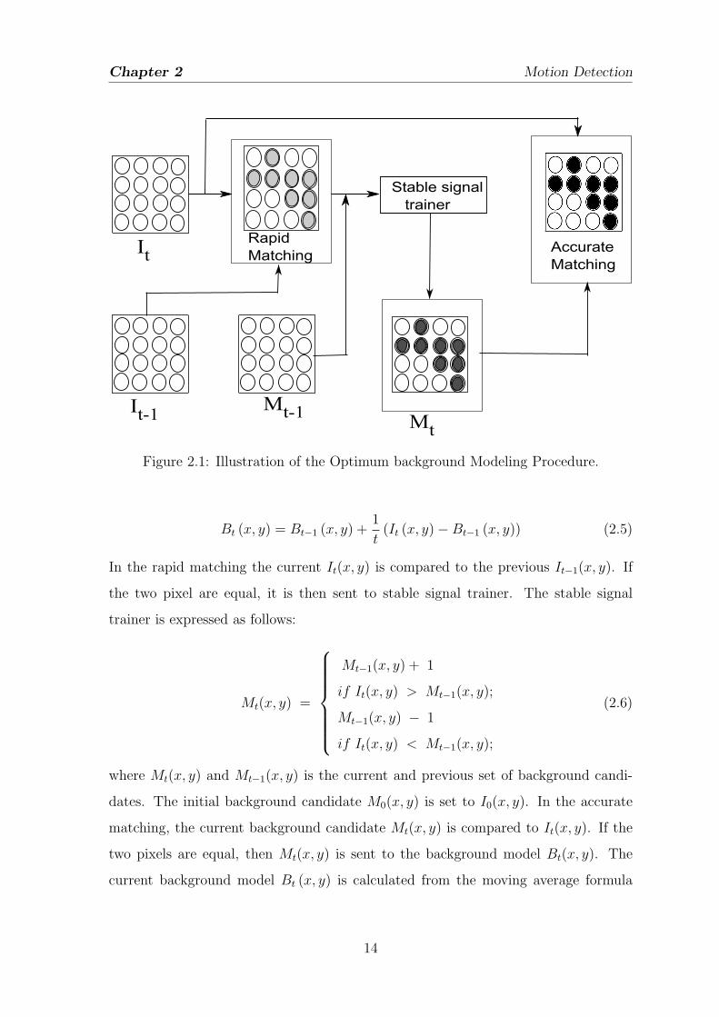
Advanced motion detection algorithm [13] uses rapid matching followed by accurate

matching to calculate the optimum background model. The initial background model

is given by the Modified Moving Average (MMA) equation computed over the K

initial frames.

13


Rapid

Matching

It-1

It

Mt-1

Mt

Stable signal

trainer

Accurate

Matching

Figure 2.1: Illustration of the Optimum background Modeling Procedure.

Bt (x, y) = Bt−1 (x, y) +1

t(It (x, y)− Bt−1 (x, y)) (2.5)

In the rapid matching the current It(x, y) is compared to the previous It−1(x, y). If

the two pixel are equal, it is then sent to stable signal trainer. The stable signal

trainer is expressed as follows:

Mt(x, y) =

Mt−1(x, y) + 1

if It(x, y) > Mt−1(x, y);

Mt−1(x, y) − 1

if It(x, y) < Mt−1(x, y);

(2.6)

where Mt(x, y) and Mt−1(x, y) is the current and previous set of background candi-

dates. The initial background candidate M0(x, y) is set to I0(x, y). In the accurate

matching, the current background candidate Mt(x, y) is compared to It(x, y). If the

two pixels are equal, then Mt(x, y) is sent to the background model Bt(x, y). The

current background model Bt (x, y) is calculated from the moving average formula

14


given below:

Bt (x, y) = Bt−1 (x, y) +1

α(It (x, y)− Bt−1 (x, y)) (2.7)

α is predefined parameter and is set experimentally to 8.

Once the proper background is generated from the updated background model,

the absolute difference is computed between the incoming video frame It(x, y) and

updated background model Bt(x, y).

t(x, y) =| It(x, y)−Bt(x, y) | (2.8)

The subtraction leaves only non-stationary or new objects, which include entire sil-

houette region of an object.

Each w × w block (i, j) within the absolute difference ∆t(x, y) is composed of

V discrete gray levels and is denoted by L0, L1, L2, L3, ..., LV−1. The block-based

probability density [13], [14] function : P(i,j)h is defined as

P(i,j)h = n

(i,j)h /w2 (2.9)

where h represents the L0, L1, L2, L3, ..., LV−1 gray level within each w × w block

(i, j), w is set at 8 and n(i,j)h /w2 denotes the number of pixels corresponding to arbi-

trary gray-level h. The block based entropy evaluation is calculated from the given

following formulae.

E(i, j) = −LV −1∑

h=0

P(i,j)h log2

(P

(i,j)h

)(2.10)

After each w×w entropy block E(i, j) is calculated, the motion block A can be defined

as follows:

A(i, j) =

1, E(i, j) > T

0, otherwise(2.11)

When the calculated entropy block (i, j) exceeds T , the motion block A(i, j) is

labeled with ’1’, denoting that it contains pixels of moving objects. Otherwise non-

15


active ones are labeled with ’0’. When the block contains pixels of moving object,

dilation and erosion is performed.

Dt(x, y) =

1, if ∆t (x, y) > Vt (x, y)

0, otherwise.(2.12)

The best variance Vt (x, y) is calculated from the given function

Vt (x, y) = N ×min(vst (x, y) , v

lt (x, y)

)(2.13)

where vst (x, y), vlt (x, y) represents the short-term variance and long-term variance. It

is calculated through the following function for ∆t (x, y) not equal to 0.

vst (x, y) =

vst−1 (x, y) + p,

if N ×∆t (x, y) > vst−1 (x, y);

vst−1 (x, y)− p,

if N ×∆t (x, y) < vst−1 (x, y);

(2.14)

vlt (x, y) =

vlt−1 (x, y) + p,

if N ×∆t (x, y) > vst−1 (x, y);

vlt−1 (x, y)− p,

if N ×∆t (x, y) < vst−1 (x, y);

(2.15)

where vst−1, vlt−1 represents the previous short-term variance and long-term variance

respectively. N is experimentally set to 2, initial vs0 and vl0 is set at ∆0 and t is a

multiple of α.

2.1.6 Simple Statistical Difference

Simple Statistical Difference method (SSD) computes the mean µx,y and the standard

deviation σx,y for each pixel (x, y) in the background image containing K images in

the time interval [t0, tk−1].

µxy =1

K

K−1∑

k=0

Ik(x, y) (2.16)

16


σxy =

(1

K

K−1∑

k=0

(Ik(x, y)− µxy)2

)1/2

(2.17)

For motion detection, absolute difference between the current image It(x, y) and

the mean µx,y from the background images is calculated.

D (x, y) =

1, if |It(x, y)− µxy| ≥ λσxy

0, otherwise(2.18)

2.1.7 W 4 background subtraction

W 4 [10] model is a simple and effective method for segmentation of foreground ob-

jects from video frame. In the training period each pixel uses three values; minimum

m(x, y), maximum n(x, y), and the maximum intensity difference of pixels in the con-

secutive frames d(x, y) for modeling of the background scene. The initial background

for a pixel location (x, y) is given by

m(x, y)

n(x, y)

d(x, y)

=

minz V z(x, y)maxz V z(x, y)maxz |V z(x, y) − V z−1(x, y)|

,

where |V z(x, y) − λ(x, y)| < 2 ∗ σ(x, y).

(2.19)

The background cannot remain same for a long period of time, so the initial back-

ground needs to be updated. W 4 uses pixel-based update and object-based update

method to cope with illumination variation and physical deposition of object. W 4

uses change map for background updation.

A detection support map (gS) computes the number of times the pixel (x, y) is

classified as background pixel.

gSt(x, y) =

gSt−1(x, y) + 1

if pixel is background;

gSt−1(x, y)

if pixel is foreground;

(2.20)

17


A motion support map (mS) computes the number of times the pixel (x, y) is

classified as moving pixel.

mSt(x, y) =

mSt−1(x, y) + 1

if Mt(x, y) = 1;

mSt−1(x, y)

if Mt(x, y) = 0;

(2.21)

where

Mt(x, y) =

1 if (|It(x, y) − It+1(x, y)| > 2 ∗ σ) ∧(|It−1(x, y) − It(x, y)| > 2 ∗ σ)

0 otherwise

(2.22)

The new background model is given by:

[m(x, y), n(x, y), d(x, y)] =

[mb(x, y), nb(x, y), db(x, y)]

if (gS(x, y) > k ∗N) then pixel − based;

[mf (x, y), nf (x, y), df (x, y)]

if (gS(x, y) < k ∗N ∧ mS(x, y) < r ∗N)

then object− based;

[mc(x, y), nc(x, y), dc(x, y)] otherwise;

(2.23)

where k and r is taken to be 0.8 and 0.1 respectively. The current pixel (x, y) is

classified into background and foreground by the following equation.

B(x, y) =

0 background

((It(x, y)− m(x, y) < kdµ

∨ (It(x, y)− n(x, y)) < kdµ)

1 foreground otherwise

(2.24)

18


2.1.8 Self-Organizing Approach to Background Subtraction

Algorithm 3: SOBS (Self-Organizing Approach to Background Subtraction)

Result: Binary mask, Bt(x, y)

Initialization1

model C for pixel I0(x, y) and store it into A2

0 ≤ c2 ≤ c1 ≤ 13

α1 =c1

max(wi,j)4

α2 =c2

max(wi,j)5


α =

α1 − tα1−α2

Kif 0 ≤ t ≤ K

α2 if t > K7

αi,j(t) = α(t)wi,j8


find best match cm in C to current sample It(x, y)10

d(pi, pj) = ||(visicos(hi), visicos(hi), vi)−11

(visicos(hi), visicos(hi), vi)||2212

d(cm, pt) = mini=1,...,n2d(ci, pt) ≤ ǫ13

ǫ =

ǫ1 if 0 ≤ t ≤ K

ǫ2 if t > K14

if cm found then15

Bt(x, y) = 016

update A in the neighborhood of cm17

for each pixel (i, j) do18

At(i, j) = (1− αi,j(i, j))At−1(i, j) + αi,jpt(x, y)19

else20

if(γ ≤ pVt

cVi≤ β

)∧(pSt − cSi ≤ τs

)∧(pHt − cHi ≤ τH

)then21

Bt(x, y) = 022

else23

Bt(x, y) = 124

19


e f

a1a2

a3

a4a5 a

6

a7a8a9

b1b2b3

b4b5b6

b7b8b9

c1 c

2c3

c4c5c6

c7c8c9

d1d2 d

3

d4d5 d

6

d7d8d9

e1e2e3

e4e5 e

6

e7e8e9

f1f2

f3

f4f5

f6

f7

f8

f9

a b c

d

Figure 2.2: Neuronal map structure of self organizing background subtraction

SOBS [9] has two phases: a calibration phase and an online phase. Calibration

consists in step from 1 to 19 and it involves neural network initial learning and con-

struction of initial background. It is run over initial K number of sequence, depends

on how many static frames are available in the video. Online phase involves neural

network adaptation and background subtraction, steps 6 to 24 are carried in online

phase and executed over t = K + 1 to Last frame in step 6.

2.1.9 Background Subtraction based on brightness and chro-

maticity distortion

Shadows cause serious problems in extracting moving objects, due to misclassification

of shadows as foreground. This work exploits the lambertian hypothesis [15] to con-

sider color as a product of irradiance and reflectance. It is based on separating the

pixel value into brightness and chromaticity distortion. Background subtraction uses

brightness and chromaticity distortion to classify pixel into foreground, background,

shadow and highlight respectively. A pixel is modeled by a 4-tuple 〈Ei, si, ai, bi〉 where

20


Ei is the expected color value, si is the standard deviation of color value, ai and bi

are the variation of brightness distortion and chromaticity distortion of the ith pixel.

The expected color value and standard deviation of ith pixel is given by

Ei = [µR (i) , µG (i) , µB (i)] (2.25)

si = [σR (i) , σG (i) , σB (i)] (2.26)

where µ (i) and σ (i) is the arithmetic means and standard deviation of pixel i, com-

puted over N background frames.

αi =

(IR(i)µR(i)

σ2R(i)

+ IG(i)µG(i)

σ2G(i)

+ IB(i)µB(i)

σ2B(i)

)

([µR(i)σR(i)

]2+[µG(i)σG(i)

]2+[µB(i)σB(i)

]2) (2.27)

CDi =

√√√√ ∑

C=R,G,B

(IC (i)− αiµC (i)

σC (i)

)2

(2.28)

αi and CDi have different distribution for different pixels. In order to use a single

threshold for every pixels, need to rescale the αi and CDi.

αi =αi − 1

ai(2.29)

CDi =CDi

bi(2.30)

where αi, CDi represents normalized brightness distortion and normalized chromatic-

ity distortion respectively. ai and bi represents the variation of the brightness distor-

tion and chromaticity distortion of the ith pixel, which is given by

ai = RMS (αi) =

√∑Ni=0 (αi − 1)

N(2.31)

bi = RMS (CDi) =

√∑Ni=0 (CDi)

2

N(2.32)

From the above equations, a pixel in the current image is classified into one of the

21


(a) (b)

(c) (d)

Figure 2.3: Results of robust background subtraction on MSA sequence (a)Originalmsa 336 frame , (b) foreground detection, (c) foreground is shown in red and shadowin blue, (d) shadow segmentation

four categories Foreground F, Background B, Shadow S, Highlight H by the following

object mask M (i) equation.

M (i) =

F : CDi > τCD or αi < ταlo, else

B : αi < τα1 and αi > τα2, else

S : αi < 0, else

H : otherwise

(2.33)

In this paper, τCD, ταlo, τα1, and τα2 are experimentally taken as 200000, −20, 6, and−6 respectively.

22


t

x

y

t

y

Figure 2.4: 3D spatial temporal video sliced along x-axis to get the 2D spatial-temporal image.

2.1.10 Background Subtraction using Fourier reconstruction

Let ft(x, y) be the 2D image of size R× C at frame t. If N frames of 2D images are

stacked along 3rd dimension then a 3D spatial-temporal image of size R×C ×N can

be constructed as f(x, y, t) = ft(x, y), where x = 0, 1, 2, ..., R− 1, y = 0, 1, 2, ..., C − 1

and t = T, T − 1, ..., T −N + 1.

Let fx(t, y) be the 2D slice of the 3D spatial-temporal image f(x, y, t) along the

x-axis [16], for y = 0, 1, 2, ..., C−1, t = T, T−1, ..., T−N+1, and x = 0, 1, 2, ..., R−1;.The 2D discrete Fourier transform (DFT) [14] of fx(t, y) is given by

Fx(u, v) =1

C.N

C−1∑

y=0

N−1∑

t=0

fx(y, t) exp

[−j2π

(uy

C+

vt

N

)](2.34)

x = 0, 1, 2, ..., R − 1

where frequency variables u = 0, 1, 2, ..., N − 1 and v = 0, 1, 2, ..., C − 1.

23


Fx(u, v) = Rx(u, v) + Ix(u, v) (2.35)

where Rx(u, v) and Ix(u, v) are the real and imaginary components of Fx(u, v)

given by:

Rx(u, v) =1

C.N

C−1∑

y=0

N−1∑

t=0

fx(y, t) cos

[2π

(uy

C+

vt

N

)](2.36)

Ix(u, v) = −1

C.N

C−1∑

y=0

N−1∑

t=0

fx(y, t) sin

[2π

(uy

C+

vt

N

)](2.37)

The power spectrum Px(u, v) of Fx(u, v) is given by

Px(u, v) = ‖Fx(u, v)‖2 = R2x(u, v) + I2x(u, v) (2.38)

When video frames are stacked along 3D, repeated vertical line pattern appears

as there are no moving objects and the background is static. The repeated vertical

line patterns in the spatial domain is seen as horizontal component in the frequency

domain. Static background can be removed by making the frequency components

along the horizontal line and center in the Fourier spectrum to zero.

Fx(u, v) = 0forN

2− ∆w

2≤ v ≤ N

2− ∆w

2(2.39)

In order to get back to the spatial domain, inverse discrete Fourier transform

(IDFT) [14] is calculated as follow:

Fx(u, v) =C−1∑

y=0

N−1∑

t=0

fx(y, t) exp

[j2π

(uy

C+

vt

N

)](2.40)

x = 0, 1, 2, ..., R − 1

The moving object in each video frame is obtained by reorganizing images as

f(x, y, t).

24


(a) (b) (c)

Figure 2.5: Motion segmentation using Fourier reconstruction (a) original image (b)gradient of image (c) foreground segmented

25


2.1.11 ICA-based background subtraction

ICA shows how the observed mixture signals X are obtained from mixing matrix A

to mix with the latent source signal S.

X = AS (2.41)

ICA solution provides solution to find out the independent signal Y , which is

very close to latent source signal S, by evaluating the demixing matrix W i,e. The

component of Y are mutually independent.

WX = Y (2.42)

ICA is used for foreground detection [17] by finding out the demixing matrix, such

that it separates the moving foreground object from the background.

yt = wXt = [w1w2][xbxf ]T (2.43)

where Xt = [xbxf ]T is data matrix, xb is the reference background image and xt is

the current image at time frame t in a video sequence. xb and xt are of size [1×mn]

obtained by resizing the 2-D image f(i, j) of size m× n as follows:

x = x((i− 1).n+ j) = f(i, j) (2.44)

i = 1, 2, ...,m; j = 1, 2, ..., n

w = [w1w2] is the demixing vector matrix for separating the foreground from the

background. As given in [17] the value of w = [0.7641−0.6452] is obtained from PSO

[18]. yt is the image containing foreground object of size [1 × mn] and needs to be

converted back to a 2D image by

Ii(u, v) = yi(u− 1).n+ v) (2.45)

u = 1, 2, ...,m; v = 1, 2, ..., n

26


(a) (b)

(c) (d)

Figure 2.6: Background segmentation using ICA model (a) Original Image, (b) back-ground subtraction, (c) gray image, (d) foreground detection

the 2D image containing separated foreground image Ii(u, v) is converted to gray-

level by

Ii(u, v)′

= Ii(u, v).c.σb + µb (2.46)

where σb, µb are the standard deviation and mean respectively, obtained from

reference background xb. c is a constant and taken as 0.5.

The pixel is classified as foreground and background by the following equation

D (u, v) =

0, if I′

i(u, v) < µI′+l.σI′

1, otherwise(2.47)

27


(a) (b)

(c) (d)

Figure 2.7: Background segmentation using ICA model (a) Original Image, (b) back-ground subtraction, (c) gray image, (d) foreground detection

28


2.1.12 A Consensus-Based Background Subtraction

Wang et al. have proposed SACON [19], which keeps a cache of N background samples

at each pixel such that xi(x, y)/i = 1, ..., N and N < t. xt(x, y) is the pixel value at

time t. To overcome the problem of background subtraction, many researcher have

used normalized color coordinates [7] given by

r = R/(R +G+ B)

g = G/(R +G+ B)

b = B/(R +G+ B) (2.48)

but this results in complete loss of intensity information, so [20], [21] have used

r, g, I coordinates and I = (R+G+B)/3. For a pixel in shadow (β ≤ It(x, y)/Ib(x, y) ≤ 1)

and for a pixel illuminated by bright light the highlight is given by (1 ≤ It(x, y)/Ib(x, y) ≤ γ)

τ ci (x, y, t) =

1 if |xct − xc

b| ≤ Tr∀c ∈ [r, g]

and α ≤ It(x, y)/Ib(x, y) ≤ γ c ∈ [I],

0 otherwise

(2.49)

Bt(x, y) =

1 if∑N

i=1 τci (x, y, t) ≥ Tn ∀c ∈ [r, g, I]

0 otherwise(2.50)

Every background sample should be adaptive to illumination variation, adapt to

new object moved or inserted in the background and it should make foreground objects

which are static for a long time to be part of the background. SACON updates its

background samples at both pixel level and blob level. Group of pixels below a certain

size are updated at pixel level. Pixel level update is done to overcome the problem of

illumination variation or small object being displaced. Pixel level update is done as

follows.

29


TOMt(x, y) = TOMt−1(x, y) + 1

ifBt(x, y) = 0

TOMt(x, y) = 0

otherwise

(2.51)

Group of pixels above a certain threshold are updated at blob level as follows

TOMt(m′

)m′∈Ω = TOMt−1(m′

)m′∈Ω + 1

ifΩisstatic

TOMt(m′

)m′∈Ω = 0

otherwise

(2.52)

2.1.13 Adaptive Background Mixture Model

A pixel at time t is modeled as mixture of K Gaussian [11] distributions. The prob-

ability of observing the current pixel value is given by

P (Xt) =K∑

i=1

wi,t ∗ η(Xt, µi,t,Σi,t) (2.53)

where wi,t, µi,t, and Σi,t are the estimate weight, mean value and covariance matrix

of ith Gaussian in the mixture at time t. η(Xt, µi,t,Σi,t) is the Gaussian probability

density function

η(Xt, µi,t,Σi,t) =1

(2π)n/2 |Σ|1/2exp− 1

2(Xt−µt)TΣ−1(Xt−µt)

Σk,t = σ2kI (2.54)

30


Algorithm 4: Mixture of Gaussian algorithm

Result: Background subtraction using Mixture of Gaussian

for each time frame t do1

for for each pixel (x, y) do2

for for each Gaussian component i = 1toK do3

if |X − µk,t| ≤ 2.5 ∗ σk,t then4

wk,t = (1− α)wk,t−1 + α (Mk,t)5

p = α/wk,t6

µk,t = (1− p)µk,t−1 + p (Xt)7

σk,t = (1− p)σ2k,t−1 + p (Xt − µk,t)

T (Xt − µk,t)8

else9

wk,t = (1− α)wk,t−110

normalize weights wk,t11

if none of the k distributions match, create new component12

Gaussians are ordered by the value of w/σ13

first B distributions are chosen as the background model14

B = argminb

(∑bk=1wk > T

)15

2.1.14 Background Subtraction in DCT Domain

A video consists of frames and each frame is divided into blocks of [8×8] in the spatial

domain. The DCT [22] is carried out in each block such that the coefficients in the

frequency domain reduces spatial redundancy. The DCT [14] is defined as

D(u, v) =7∑

x=0

7∑

y=0

F (x, y)Γu,v(x, y), u, v = 0, 1, ..., 7 (2.55)

where F (x, y), x, y = 0, 1, ..., 7, is the pixel value in the block, D(u, v) is the

corresponding DCT frequency of the block. Γu,v(x, y) is the basis matrix for DCT.

31


Γu,v(x, y) = ϕ(u)ϕ(v) cos(π(2x+ 1)u/16)× cos(π(2y + 1)v/16) x, y = 0, 1, ..., 7

(2.56)

where ϕ(s) = 0.5/√2, if s = 0; ϕ(s) = 0.5 otherwise.

If we stack the matrix F into column wise, the resulting matrix f is [64× 1] and

if dct, of f is taken, it results in d of size [64× 1]. K is [64× 64] kernel matrix.

d = Kf (2.57)

DCT is orthogonal transform, its IDCT can be given by

f = KTd (2.58)

where KT denotes the transpose of the matrix K.

DtB = dBt,k, k = 1, 2, ..., L is the DCT coefficients at time t, where dBt,k is 64-

dimensional background vector for the kth pixel block at time t, L is the number

of block in a frame

Running Average Algorithm in the DCT Domain

The RA algorithm in the DCT domain for calculation of background is given by

dBt,k =Bt,k +(1− α)dBt−1,k, k = 1, 2, ..., L (2.59)

dBt,k and dBt−1,k is the background estimation of size [64× 1] at current time frame

t and previous frame t− 1 respectively for the kth block. where k = 1, 2, ..., L and L

is the number of blocks in the image. α is the learning rate for the RA algorithm.

Median Algorithm in the DCT domain

For the median algorithm in the dct domain, each kth block’s dc coefficient of DCT

in the time frame l = t, t−∆t, ..., is calculated and then out of them mid value is find

out. Current background dBt,k is given as follows:

32


Algorithm 5: Median based algorithm

Result: Computation and storage of median based background

for each time frame t do1

for for each block k = 1, 2, ..., L do2

st,k = argmid (DCl,k, l = t, t−∆t, ..., )3

if st,k 6= st−1,k then4

dBt,k = dst,k,k5

DtB = dBt,k, k = 1, 2, ..., L6

MoG Algorithm in DCT Domain

The MoG algorithm can be modeled in the DCT domain, as 64-dimensional vector

for block k = 1, 2, ..., L and each block contains i = 1, 2, ...,M number of component.

M is taken as 3 to 5 and it depends on computations memory.

Pr(dk|λk) =M∑

i=1

wk,iGi(dk) (2.60)

where dk is a 64-dimensional DCT coefficient vector for block k, wk,i is the weight of

the block k and i denotes the number of Gaussian component. Gi(dk) is the Gaussian

component density given by:

Gi(dk) = 1/((2π)32σ64k,i)× exp(−(dk − µk,i)

T (dk − µk,i)/(2σ2k,i)) (2.61)

where µk,i and σk,i are the 64-dimensional mean and variance vector for the block

k in the i th component.

A block is said to be matching, if it satisfies the following condition.

(dk − µk,i)T (dk − µk,i) < ς tk,i (2.62)

For those matching block k in the frame at time t, matching component is given

by :

33


i = argi min(dk − µk,i)T (dk − µk,i)/ς

t−1k,i (2.63)

where ς t−1k,i is said to be the matching threshold. and then the weight, mean and

variance of the matched Gaussian component i is updated by the following equation

wtk,i

= (1− α)wt−1

k,i+ α (2.64)

µtk,i

= (1− ρ)µt−1

k,i+ ρdtk (2.65)

ς tk,i

= (1− ρ)µt−1

k,i+ ρ(dk − µk,i)

T (dk − µk,i) (2.66)

where α is the learning rate and is usually taken to be (0 < α < 1) and ρ = α/wtk,i.

For those un-matched components, only the weight wtk,i

are updated as follows:

wtk,i

= (1− α)wt−1

k,i(2.67)

If the block doesn’t satisfies the equation 2.63, the Gaussian component weight is

replaced with the minimum weight, mean is replaced with the current value of the

block and matching threshold is replaced with initial value. Finally the weights of all

Gaussaian component are normalized.

The first S Gaussian components are chosen as background model, and S is given

by

S = argb min(

ib∑

l=i1

> T ) (2.68)

where T is a threshold.

Moving Object Segmentation

In the block k at the current time frame t, moving object inside the block k is detected

by the euclidean distance between the dt,k and dBt,k

34


(a) (b)

(c) (d) (e)

Figure 2.8: Background subtraction using dct (a) Original Image, (b) ground-truth,(c) RA (DCT), (d) Median (DCT), (e) MoG (DCT)

Ωt,k =∥∥dt,k − dBt,k

∥∥2, k = 1, 2, ..., L (2.69)

if Ωt,k > τ , where τ is a threshold, the block k at the current time frame t is

classified as foreground block. In order to classify, foreground block as foreground

pixel the following relation should hold.

(dY (x, y) > T(Y )h ) ∨ (dCb(x, y) > T

(Cb)h ) ∨ (dCr(x, y) > T

(Cr)h ) (2.70)

or

(dY (x, y) > T(Y )l ) ∧ (dCb(x, y) > T

(Cb)l ) ∧ (dCr(x, y) > T

(Cr)l ) (2.71)

where (dY (x, y), (dCb(x, y), (dCr(x, y) is the absolute difference of pixels in the

spatial domain between current frame and the background . T(c)l , T

(c)h , c ∈ Y,Cb, Cr

are the low and high threshold for the color coordinate c.

35


Waving tree [23] RA Median MoGRecall 0.9851 0.9841 0.9842Precision 0.8153 0.8670 0.8718F1 0.9928 0.9219 0.9246Similarity 0.8054 0.8551 0.8598

Table 2.1: Pixel-based accuracy result for background subtraction in DCT

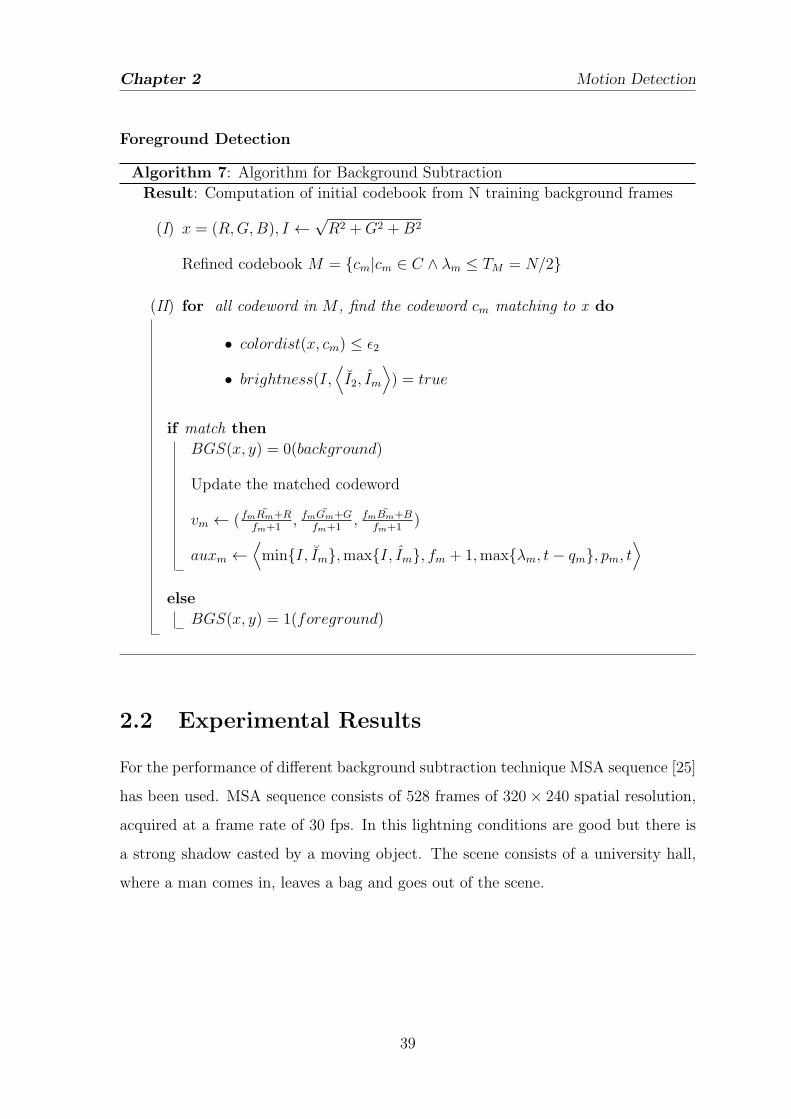
2.1.15 Background Subtraction using Codebook Model

Background subtraction using codebook (CB) [24] is an efficient algorithm that can

handle illumination variation and background motion due to periodic motion in the

leaves of trees.

Construction of the Initial Codebook

Let χ = x1, x2, ..., xN represent training sequence for a pixel consisting of initial N

background frames for an RGB vector and C = c1, c2, ..., cL denotes the codebook

for the pixel having L codewords. Each pixel has a different length of codebook,

depending on its pixel variation. Each codeword ci, i = 1, ..., L has RGB vector

vi = (Ri, Gi, Bi) and it also consists of 6-tuple auxi =⟨Ii, Ii, fi, λi, pi, qi

⟩. Where

Ii, Ii gives the min and max brightness, respectively, of all pixel assigned to this

codeword. The frequency of occurrence of the codeword is denoted as f . λ represents

the longest interval during the training of background frames that the codeword has

not recurred. p, q is the first and last access that the codeword has occurred.

36


Algorithm 6: Algorithm for Codebook construction

Result: Computation of initial codebook from N training background frames

(I) Initialization: L← 01, C ← φ

(II) for each t = 1 : N do

if C = φ thenL← L+ 1

vL ← (R,G,B), auxL ← 〈I, I, 1, t− 1, t, t〉.

(i) xt = (R,G,B), I ←√R2 +G2 + B2

(ii) find the codeword cm matching to xt given by the two condition

(a) colordist(xt, vm) ≤ ǫ1

(b) brightness(I, (Im, Im)) = true

(iii) if match then

vm ← (fmRm+Rfm+1

, fmGm+Gfm+1

, fmBm+Bfm+1

)

auxm ←⟨minI, Im,maxI, Im, fm + 1,maxλm, t− qm, pm, t

⟩

(iv) elseL← L+ 1

vL ← (R,G,B)

auxL ← 〈I, I, 1, t− 1, t, t〉.

(III) for codeword ci, i = 1, ..., L, do

λi ← maxλi, (N − qi + pi − 1).

Color and Brightness Distortion

pixel xt is said to be matching the codeword cm in C = ci|1 ≤ i ≤ L if it satisfies

the following equations.

colordist(xt, vm) ≤ ǫ1 (2.72)

37


brightness(I, (Im, Im)) = true (2.73)

Color Distortion

Let xt = (R,G,B) be the input pixel and the codeword be ci where vi = (Ri, Gi, Bi)

∥∥x2t

∥∥ = R2 +G2 + B2 (2.74)

∥∥v2i∥∥ = R2

i + G2i + B2

i (2.75)

〈xt, vi〉2 = (RiR + GiG+ BiB)2 (2.76)

The color distortion δ can be computed by the following equations.

p2 = ‖xt‖2 cos2 θ =〈xt, vi〉2

‖vi‖2(2.77)

colordist(xt, vi) = δ =

√‖xt‖2 − p2. (2.78)

Brightness Distortion

Each codeword has a range has a range given by

Ilow = αI, Ihigh = min

βI,

I

α

(2.79)

where α < 1 and β > 1. The value of α is taken between 0.4 and 0.7 and β is between

1.1 and 1.5. The brightness distortion is calculated as follows:

brightness(I,⟨

I ,

I⟩) =

true if Ilow ≤ ‖xt‖ ≤ Ihigh,

false otherwise.(2.80)

38


Foreground Detection

Algorithm 7: Algorithm for Background Subtraction

Result: Computation of initial codebook from N training background frames

(I) x = (R,G,B), I ←√R2 +G2 + B2

Refined codebook M = cm|cm ∈ C ∧ λm ≤ TM = N/2

(II) for all codeword in M , find the codeword cm matching to x do

• colordist(x, cm) ≤ ǫ2

• brightness(I,⟨I2, Im

⟩) = true

if match then

BGS(x, y) = 0(background)

Update the matched codeword

vm ← (fmRm+Rfm+1

, fmGm+Gfm+1

, fmBm+Bfm+1

)

auxm ←⟨minI, Im,maxI, Im, fm + 1,maxλm, t− qm, pm, t

⟩

else

BGS(x, y) = 1(foreground)

2.2 Experimental Results

For the performance of different background subtraction technique MSA sequence [25]

has been used. MSA sequence consists of 528 frames of 320× 240 spatial resolution,

acquired at a frame rate of 30 fps. In this lightning conditions are good but there is

a strong shadow casted by a moving object. The scene consists of a university hall,

where a man comes in, leaves a bag and goes out of the scene.

39


2.2.1 Accuracy Metrics

For measuring accuracy, different metrics such as precision, Recall, F1, and Similarity

is calculated and tested with msa.1130, msa.1266, msa.1296, and msa.1336 sequence

of MSA video.

Recall =tp

tp + fn(2.81)

Precision =tp

tp + fp(2.82)

Recall =2 ∗Recall ∗ Precision

Recall + Precision(2.83)

Similarity =tp

tp + fn + fp(2.84)

W4 (frame) → 130 266 296 336Recall 0.9991 0.9986 0.9988 0.9995Precision 0.9991 0.9934 0.9939 0.9865F1 0.9928 0.9960 0.9963 0.9930Similarity 0.9856 0.9920 0.9927 09860

Table 2.2: Pixel-based accuracy result for W4

SOBS (frame) → 130 266 296 336Recall 0.9979 0.9973 0.9979 0.9977Precision 0.9989 0.9976 0.9979 0.9973F1 0.9984 0.9974 0.9979 0.9975Similarity 0.9967 0.9949 0.9958 0.9950

Table 2.3: Pixel-based accuracy result for SOBS

40


RBS (frame) → 130 266 296 336Recall 0.9981 0.9976 0.9984 0.9984Precision 0.9917 0.9931 0.9937 0.9888F1 0.9949 0.9953 0.9960 0.9936Similarity 0.9899 0.9907 0.9920 0.9872

Table 2.4: Pixel-based accuracy result for RBS

ICA (frame) → 130 266 296 336Recall 0.9981 0.9965 0.9974 0.9975Precision 0.9897 0.9960 0.9960 0.9971F1 0.9938 0.9962 0.9967 0.9973Similarity 0.9878 0.9925 0.9934 0.9947

Table 2.5: Pixel-based accuracy result for ICA

SACON (frame) → 130 266 296 336Recall 0.9942 0.9918 0.9921 0.9911Precision 0.9974 0.9969 0.9976 0.9963F1 0.9958 0.9944 0.9949 0.9937Similarity 0.9917 0.9888 0.9898 0.9874

Table 2.6: Pixel-based accuracy result for SACON

MoG (frame) → 130 266 296 336Recall 0.9994 0.9814 0.9780 0.9917Precision 0.9749 0.9969 0.9998 0.9605F1 0.9870 0.9891 0.9888 0.9759Similarity 0.9743 0.9783 0.9778 0.9529

Table 2.7: Pixel-based accuracy result for MoG

CB (frame) → 130 266 296 336Recall 0.9978 0.9973 0.9979 0.9976Precision 0.9988 0.9979 0.9981 0.9969F1 0.9983 0.9976 0.9980 0.9972Similarity 0.9967 0.9952 0.9960 0.9945

Table 2.8: Pixel-based accuracy result for CB

41


(a) (b) (c)

Figure 2.9: (a) MSA image (b) ground truth (c) W4 result

42


(a) (b) (c)

Figure 2.10: (a) MSA image (b) ground truth (c) SOBS result

43


(a) (b) (c)

Figure 2.11: (a) MSA image (b) ground truth (c) Result of robust background sub-traction using brightness and chromaticity distortion

44


(a) (b) (c)

Figure 2.12: (a) MSA image (b) ground truth (c) ICA result

45


(a) (b) (c)

Figure 2.13: (a) MSA image (b) ground truth (c) SACON result

46


(a) (b) (c)

Figure 2.14: (a) MSA image (b) ground truth (c) MOG result

47


(a) (b) (c)

Figure 2.15: (a) MSA image (b) ground truth (c) CB result

48

Chapter 3


In visual surveillance system, motion detection is the crucial and important step that

classifies the moving foreground object from the background. The segmented moving

foreground object may be humans, vehicles, animals, flying birds, moving clouds,

leaves of a tree, or any other noise etc. The job of a classification stage in the visual

surveillance system, is to classify the moving foreground object into predefined classes

such as single person, group of person, or vehicle, etc. The visual surveillance system

is mostly used for humans and vehicles. Once the foreground object belongs to this

class, the latter task such as personal identification, object tracking, and activity

analysis of the detected foreground object can be done much more efficiently and

accurately. The object classification is a standard pattern recognition problem and

there are two approaches for classifying [1] moving foreground objects.

1. Shape-based classification: In shape-based classification, the moving fore-

ground object region such as points, boxes, silhouettes and blobs are used for

classification. Lipton et al. [4] have used image blob dispersedness and area to

classify moving foreground object into human, vehicles and noise. If a target

is present over a longer duration in the video, then the chances of having fore-

ground object are high and if it is for short duration, then it is cluttered and is

due to the noise in the frame. Dispersedness of an object is calculated from the

given formulae.

49

Chapter 3 Object Classification

Dispersedness =Perimeter2

Area(3.1)

Human body shape is complex in nature and will have more dispersedness than

a vehicle. So the humans can be classified from vehicle using dispersedness and

they have use Mahalanbois distance-based segmentation for foreground object

classification.

2. Motion-based classification: The human body is non-rigid and articulated.

It shows periodic motion and this property of human can be used for classi-

fication from the rest of foreground objects in the video frame. Cutler et al.

[26] tracked interested object and its self-similarity is computed over time. For

a periodic motion, computed self-similarity is also periodic. Time frequency

analysis is done to detect and characterize the periodic motion.

3.1 Silhouette Template Based Classification

First the object to be classified is detected and segmented from video using back-

ground subtraction technique. In silhouette template based classification foreground

object distance signal is computed and its similarity with the stored templates of the

foreground object is found using the minimum distance and is classified into group

such as human, group of humans, vehicle, and animals. The object classification is

done by a two step method as follows:

Offline step: In the offline step, various objects such as humans, group of humans,

vehicles and animals distance signal is computed and stored in the template database.

Online step: The object silhouette is extracted in each frame and its distance

signal is computed from it. The computed distance signal is then compared with the

template distance signal stored in the database. The template is then classified to the

group which gives the minimum distance with the current foreground object.

50


(a) (b) (c)

Figure 3.1: Illustration of object silhouette. (a) Original image (b) segmented fore-ground (c) object silhouette.

(a)

(b)

Figure 3.2: Template database of human and vehicles (a) human (b) vehicles.

3.2 Object Silhouette Extraction

First step in object classification is to extract the silhouette of the foreground object.

Silhouette extraction is required both in storing the template of the database (offline)

and in matching the distance signal computed from the silhouette of the foreground

object with the template distance signal stored in the database. In silhouette extrac-

tion, first foreground object is segmented using background subtraction technique and

then boundary following algorithm is done. Foreground object’s centroid is computed

(xc, yc), by choosing this centroid as the reference origin, the outer contour [3] is traced

in counterclockwise to turn into a 1 −D distance signal S = d (1) , d (2) , ..., d (N)by the given equation.

51


(a)

0 50 100 150 200 250 300 3500

10

20

30

40

50

60

70

Number of points

Dis

tanc

e S

igna

l

(b)

0 20 40 60 80 1000

0.1

0.2

0.3

0.4

0.5

0.6

0.7

0.8

0.9

1

Number of points

Nor

mal

ized

dis

tanc

e S

igna

l

(c)

Figure 3.3: Original Image silhouette and its corresponding original distance andnormalized distance signals. (a) object silhouette. (b) original distance signal. (c)normalized distance signal.

52


d (i) =√(x (i)− xc)2 + (y (i)− yc)2 (3.2)

In different frames of a video, the size of object changes, so 1−D signal of same

object will vary from one frame to another. To eliminate the influence of signal length

and spatial scale [3], [27], 1−D signal length and magnitude is normalized. The 1-D

signal is normalized in length by

S = d

(i ∗ N

C

), ∀i ∈ [1, ..., C] (3.3)

where C denotes the fixed length signal and N is the original signal length. The

corresponding normalized length signal is normalized in magnitude by

S (i) =S

max(S)(3.4)

Figure 3.3 shows object silhouette and its corresponding original distance and

normalized distance signal.

3.3 Target Classification

The classification metric used to classify object is similarity of object shape [27]. In

order to classify the foreground object into predefined classes the minimum distance

is computed between the template and the foreground object as given by

DistAB =C∑

i=1

|SA (d(i))− SB (d(i))| (3.5)

53

Chapter 4

Object Tracking

4.1 Introduction

Object tracking, consists in estimating the trajectory of moving objects in the video

sequence. Automatic detection and tracking of moving object is very important task

for human-computer interface, video communication, security and surveillance system

application and so on. Here in this chapter, we use vision system to monitor activity

in a place over an extended period of time. It provides a robust mechanism to find

out the suspicious activities in and around the site and is very beneficial for the

defense people in detecting intruders. Video surveillance can be used in monitoring

the safe custody of crucial data, arms and ammunition in defense establishments. It

can provide security to key installations and monuments.

It uses infrared sensors [28] to locate and track the direction of the moving object

and sends out a trigger signal to video cameras for tracking. Video cameras are not

always taking the video image of the site, it starts acquisition image only when it

gets triggered signal from the infrared sensor. In this way this system uses less data

for storing the video imagery. Infrared sensors are connected to sensor node and it

is further connected to gateway as shown in Fig. 4.1. Inter-connection can be wired

or wireless connection. Video surveillance cameras are connected to the gateway.

The gateway is used as communication and information processing unit to process

the information obtained from the infrared sensors and video cameras. Gateway is

54

Chapter 4 Object Tracking

Figure 4.1: Video surveillance cameras, infrared sensor, sensor node and gateway insensor network for intelligent tracking

a medium to communicate the video cameras and infrared sensors with the central

database system, using Internet and WLAN (Wireless Local Area Network).

Every object tracking systems starts with detecting moving object in video streams.

Motion segmentation not only helps in segmenting moving region from the rest of

image, detecting moving objects is used for recognition, classification and activity

analysis, making these latter steps more efficient. The detection of motion in many

tracking systems relies on the techniques of frame differencing and background sub-

traction. Frame differencing is a pixel-wise differencing between two or three consec-

utive frames in an image sequence to detect regions corresponding to moving object

such as human and vehicles. On the other hand, background subtraction detects

moving regions in an image by taking the difference between the current image and

the reference background image captured from a static background during a period

of time.

The major problems encountered in the object tracking [29] are changes in illumi-

nation, complex object shape being tracked and occlusion in case of tracking multiple

55


people. Some of the difficulties in tracking moving objects can be summarized as

follows.

• Loss of information in projecting the 3-D image to 2-D plane,

• Noise in image video resulting in loss of information,

• Difficulty in finding the exact position of moving object in each frame,

• Partial and full object occlusions due to object or structure present in the scene,

• Complex shapes of object,

• Unobstructed view of background is not available,

• Motion in the background,

• Varying illumination condition,

• Need for real-time processing.

In object detection methodology, many researchers have developed their methods.

Changes in scene lightning can cause problem for object detection. Stauffer and

Grimson [11] have modeled each pixel as a mixture of Gaussians and uses an on-line

approximations to update the model. This can deal with lightning changes, motions in

the background, and from the long term scene changes. Maddalena and Petrosino [9]

have proposed SOBS based on self organization through artificial neural networks that

can handle background clutter, gradual illumination variations and camouflage, has no

bootstrapping limitations, overcomes the problem of shadows cast by moving objects,

and achieves robust detection for different types of videos taken from still cameras.

Toyoma et al. [8] have discussed the problems of changing illumination, background

clutter, camouflage and shadows, using the proposed three-component system for

background maintenance: the pixel level component, the region-level component and

the frame-level component.

56


Homomorphic

Filtering

Input

Video

Output

Video

Gamma

Correction

Frame

Differencing

Morophological

Operation

Image

Labelling

Object

Representation

Figure 4.2: Steps in object tracking under varying illumination condition

4.2 Object Tracking under Varying Illumination

Condition

In this section, a robust object tracking [30] algorithm is proposed to overcome the

problem of illumination variation. It is proposed to detect and track a moving object

using frame differencing. Frame differencing method is one of the simplest methods

to detect and track objects for real time processing. Object detection and tracking in

each frame of the video is performed by a six stage process shown in Fig.4.2.

The various sub-processes are described below.

4.2.1 Homomorphic Filtering

The input video is decomposed into frames f(x, y, n) and each frame is converted into

grayscale image. Here x, y are the spatial coordinates and n is the frame number that

represents discrete time. A video image may be modelled as :

f(x, y, n) = i(x, y, n)× r(x, y, n) (4.1)

where i(x, y, n) and r(x, y, n) denote the illumination and reflectance components

respectively. The nature of i(x, y, n) is determined by the illumination source and

r(x, y, n) is determined by the characteristics of the object to be imaged. The param-

eters will have a range of:

0 < i(x, y, n) <∞ (4.2)

57


ln DFT H(u,v) IDFT expf(x,y)

g(x,y)

Figure 4.3: Homomorphic filtering

and

0 < r(x, y, n) < 1 (4.3)

To overcome the problem of varying illumination condition, homomorphic filtering

is employed here. This filtering process is depicted in Fig. 4.3. The process is

performed in log domain and hence a log-transformation at the beginning and an

exponentiation at the end are a must. A definite high-pass filter, characterized by its

frequency-domain transfer-function H(u, v),is employed to reject very low frequency

components that usually represent illumination variation. To perform this frequency-

domain filtering, signal is transformed to frequency-domain. Hence the DFT and

inverse-DFT processes are employed as shown in the figure.

The illumination component of an image has slow spatial variations,while the re-

flectance component tends to vary rapidly. The problem with low cost surveillance

camera is that their video imagery gets affected by the changing illumination condi-

tion. A good control over the illumination and reflectance components can be done

with homomorphic filter.

Homomorphic filter function H(u, v, n) is given by

H(u, v, n) = (γH − γL)[1− e−c[D2(u,v,n)/D20 ]] + γL (4.4)

where

D(u, v, n) = [(u− P/2)2 + (v −Q/2)2]1/2 (4.5)

Here u and v denote frequency-domain variables and typically P = 2M and Q = 2N

are chosen, for frame size of M ×N . Constant c controls the sharpness of the slope of

the function as it makes transition between γL and γH and D0 is the cut-off frequency.

γL < 1 and γH > 1 are chosen to attenuate the contribution made by the low fre-

quencies (illumination) and amplify the contribution made by high frequencies (re-

58


flectance). As a result dynamic range is compressed and contrast is enhanced.

4.2.2 Gamma Correction

Gamma correction is a nonlinear operation used to code and decode luminance in

video or still image systems. Gamma correction is defined by the following power-law

expression:

s = crγ (4.6)

where c and γ are positive constants. A gamma value γ < 1 is sometimes called

an encoding gamma, and the process of encoding with this compressive power-law

nonlinearity is called gamma compression. Conversely a gamma value γ > 1 is called

a decoding gamma and the application of the expansive power-law nonlinearity is

called gamma expansion.

4.2.3 Frame Differencing

Frame differencing is a pixel-wise difference between two consecutive frame. Each

current frame is subtracted from the previous frame to detect the moving object.

This is being used to detect regions corresponding to moving object such as humans

and vehicles. Frame differencing is very adaptive to changing environments, but very

often holes are left inside moving entities. It depends on good threshold to segment

moving foreground from the background. Threshold T should be judiciously selected.

If the difference is greater than the threshold T , then the value is considered to be a

part of the moving object; otherwise, it is considered to be the background. Here a

threshold T is chosen based on Otsu’s [31] method. Otsu’s method is optimum in the

sense that it maximizes the between-class variance of the background and foreground.

D (x, y, n) =

1, if |f(x, y, n)− f(x, y, n− 1)| ≥ T

0, otherwise(4.7)

It works only when there is no camera motion, the moving object is not stationary

and it is not occluded.

59


4.3 Object Tracking under Background Clutter

In this section, we aim to develop a robust method to handle problem related to non-

stationary background such as branches and leaves of trees by decreasing spatial and

intensity resolution of the video imagery. It is proposed to detect and track a moving

object using frame differencing. It is one of the simplest real time processing methods

to detect moving object and Fuzzy c-means (FCM) clustering is used to segment the

foreground object and the background into two clusters. FCM algorithm classifies the

image by grouping similar data points in the feature space into clusters.

Till now, there is no research reported on object tracking by reducing spatial

and intensity resolution of image under background clutter. Here a novel and robust

scheme is proposed [32] to track an object, with web camera, in presence of background

clutter by reducing spatial and intensity resolution. Once three frame differencing is

done, FCM algorithm is used to separate the foreground object from the background.

We have modified the work carried by Sugandi et al. [33]. Here image frames

obtained from the frame differencing is not directly used for AND operation. Rather

the two frames acquired, as shown in Fig.4.4, are used for filtering operation. The

two frames are operated individually with morphological operation, FCM clustering

and then image thresholding. Finally, the thresholded images of these two channels

are ANDed and the object’s position is identified. The results obtained by perform-

ing these steps are better than directly carrying out AND operation after the frame

differencing and then doing filtering operation as proposed in [33].

4.3.1 Median Filtering

Smoothening of gray video imagery is done using median filter [14]. It is being done to

reduce noise and increase the performance of detecting moving object. Median filter

is operated with m× n pixels. Here m× n specifies the size of window. Median filter

replaces the value of a pixel by the median of the intensity values in the neighborhood

of that pixel in the window of m× n.

60


Capture three consecutive

frames

Frame fn

Frame f n+1

Median filtering

Reduce spatial and

intensity resolution

Difference

image

Frame difference

Gray scaling

Frame f n-1

Difference

image dn-1

Image

thresholding

IImage

thresholding

Morphological

operation

Morphological

operation

and

Difference

image dn+1

Fuzzy c-means

clustering

Fuzzy c-means

clustering

AND operation

Object representation

Input Video

Output Video

Figure 4.4: Steps in object tracking under background clutter

4.3.2 Reduction in Spatial and Intensity Resolution

Non-stationary background such as branches and leaves of trees is considered to be

part of the background. But this non-stationary background is often considered as a

fake motion other than the motion of the object of interest and it causes the failure

61


(a) (b) (c) (d)

Figure 4.5: Reducing spatial resolution of an image (a) Original image (640 × 480pixels), (b)160× 120 pixels, (c) 80× 60 pixels, (d) 40× 30 pixels.

(a) (b) (c) (d)

Figure 4.6: Reducing intensity resolution of an image (a) Original image (8−bit) (b)7−bit (c) 6−bit (d) 5−bit (e) 4−bit (f) 3−bit (g) 2−bit (h) 1−bit representation

of detection of the object. To overcome the problem of non-stationary background,

we reduce the spatial and intensity resolution.

(i) Spatial Resolution: In reducing spatial resolution [14], [33] of the image, the

image size is kept constant. Here spatial resolution of image is done by aver-

aging pixels value of its neighbors, including itself. We use a video image with

resolution 640 × 480 pixels. The original image size is 640 × 480 pixels. After

62


applying the low resolution image, the numbers of pixels is reduced to 160×120,80 × 60, or 40 × 30 pixels, respectively as shown in Fig. 4.5, while the image

size is still 640× 480 pixels.

(ii) Intensity Resolution: In reducing intensity resolution [14], the number of bits

used to represent the image is reduced from k = 7 to k = 1 as shown in

Fig. 4.6 while keeping the image size constant at 640 × 480 pixels. The 256−,128−, 64−, and 32− level images are visually identical. In 16− level there is

insufficient number of intensity levels for representing an digital image. Image

size of 640× 480 pixels is reduced to 40× 30 pixels and with 64 intensity levels,

the proposed algorithm sensibly tracks the moving object.

The spatial and intensity reduced resolution image is used to lessen the scattering

noise and small fake motion in the background because of non-stationary background

such as leaves of trees. The noise due to the non-stationary backgrounds have small

motion region and it disappears in spatial and intensity reduced image.

4.3.3 Frame Differencing

Frame difference method is performed on the three successive frames, which are be-

tween frame fn and fn−1 and between frame fn+1 and fn. This is being used to detect

moving object and to find out the regions which have changed.

dn−1 = |fn − fn−1|

dn−1 = |fn+1 − fn| (4.8)

It works only when there is no camera motion and the moving object is not oc-

cluded or the object has not stopped motion.

63


4.3.4 Fuzzy C-Means Clustering

Fuzzy c-means (FCM) [34], [35] clustering is an unsupervised technique that classifies

the image with N pixels (x1, x2, ..., xN ) by grouping similar data points in the feature

space into c clusters. The FCM algorithm assigns pixels to each group by using fuzzy

memberships. The grouping is made by iteratively minimizing the cost function which

is dependent on the distance of the pixels to the cluster centers in the feature domain.

The criterion function used for fuzzy C-means clustering is given by

J =N∑

j=1

c∑

i=1

umij ‖xj − vi‖2 (4.9)

where uij represent the membership of pixel xj in the ith cluster, vi is the ith

cluster center, ‖·‖ is a norm metric, and m is constant. The parameter m controls

the fuzziness of the resulting position. The membership function and cluster centers

are updated by 4.10 and 4.11.

uij =1

∑ck=1

‖xj−vi‖

‖xj−vk‖

2m−1

(4.10)

and

vi =

∑Nj=1 u

mijxj∑N

j=1 umij

(4.11)

FCM starts with an initial guess for the cluster centers and converges to solution

of cluster center vi .

4.3.5 Image Thresholding

The result obtained from the FCM algorithm is used for thresholding, foreground

object from the background. Thresholding [14], [31] is an important technique for

image segmentation based on the assumption that the objects can be distinguished

and extracted from the background. Once image thresholding is done then labeling is

done to label moving object emerging in the background. The connected component

labeling groups the pixels into components based on pixel connectivity. In this labeling

64


connected component is done through four neighbors.

4.3.6 AND Operation

mn = dn−1 ∩ dn+1 (4.12)

AND operation is performed to find out the similarity between the two difference

frames dn−1 and dn+1. By this operation, the uncorrelated noise present in the two

frames is removed.

4.4 Filtering

4.4.1 Morphological Operation

Morphological operations [14] apply a structuring element to an input image, creat-

ing an output image of the same size. Morphological operation is performed to fill

small gaps inside the moving object and to reduce the noise remained in the moving

objects. The morphological operators implemented are dilation followed by erosion.

In dilation, each background pixel that is touching an object pixel is changed into an

object pixel. Dilation adds pixels to the boundary of the object and closes isolated

background pixel. Dilation of set A by structuring element B [14] is defined as :

A⊕B =⋃

b∈B

(A)b (4.13)

In erosion, each object pixel that is touching a background pixel is changed into

a background pixel. Erosion removes isolated foreground pixels. Erosion of set A by

structuring element B [14] is defined as:

A⊖B =⋂

b∈B

(A)−b (4.14)

The number of pixels added or removed from the objects in an image depends on

the size and shape of the structuring element used to process the image. Morphological

65


operation eliminates background noise and fills small gaps inside an object. This

property makes it well suited to our objective since we are interested in generating

masks which preserve the object boundary. There is no fixed limit on the number

of times dilation and erosion is performed. In the proposed algorithm dilation and

erosion is used iteratively till the foreground object is completely segmented from the

background.

4.4.2 Image Labeling

After foreground region detection, a binary connected component analysis is applied to

the foreground pixels to assign a unique label to each foreground object. Connected

component labeling [14] is performed to label each moving object emerging in the

background. The connected component labeling groups the pixels into components

based on pixel connectivity. Connected component labeling is done by comparing the

pixel with the pixel in four neighbors. If the pixel has at least one neighbor with the

same label, this pixel is labeled as same as neighbors label.

4.5 Object Representation

Once morphological operations are over, the detected foreground object is fully visible

from the background and there is less chance of misdetection of object. The segmented

object is represented through centroid and rectangular shape to envelope the object.

Following formulae are used to determine a centroid

Cx(n) = l(n)/2 (4.15)

Cy(n) = b(n)/2 (4.16)

where l(n) and b(n) are derived as follows:

l(n) = x(n)max − x(n)min (4.17)

b(n) = y(n)max − y(n)min (4.18)

66


Here l(n) and b(n) are length and breadth of the rectangular region that describes

the detected foreground and x(n)max ,x(n)min , y(n)max , x(n)min are the maximum

and minimum spatial coordinates of the detected foreground region.

4.6 Object Tracking using Correlation Metrics

4.6.1 Correlation metrics

Let us consider a template w and a image f , over which search for an object template

needs to be carried out is an graylevel image. The position of the object can be

detected by finding out the correlation of template w with every template size selection

in the image f . The template w is of size K × L and image f is of size M ×N .

The standard 2−D correlation metric is given by:

c(m,n) =K−1∑

i=0

L−1∑

j=0

f(m+ i, n+ j)w(i, j) (4.19)

where c(m,n) is the element of the correlation matrix at row m = 0, 1, 2, ...,M −K + 1 and column n = 0, 1, 2, ..., N − L+ 1.

The standard correlation in frequency domain is given as:

c = real(ifft(F. ∗W ∗)) (4.20)

where F and W are the 2-D discrete Fourier Transforms(DFT) of f and w, respec-

tively. Before computing the DFT, f and w must be properly padded [14], [36] to

avoid wraparound error. The minimum size of the zero-padded images should be

P ×Q, where P ≥M +K − 1 and P ≥ N + L− 1.

The correlation of the template with the image, gives a maximum value at (m∗, n∗),

which is the top-left corner of the template’s best match with the image. This cor-

relation metric performance is effected in the varying illumination condition and the

values of the correlation metrics are not in the range of [−1.01.0].However, normalize correlation [36] is less effected by the varying illumination

condition and its values are normalized by the square-roots of the energies of the

67


image and template. Its values are in the range of [−1.01.0]. Normalize correlation is

given by:

c(m,n) =

∑K−1i=0

∑L−1j=0 f(m+ i, n+ j)w(i, j)

√∑K−1i=0

∑L−1j=0 f(m+ i, n+ j)2

√∑K−1i=0

∑L−1j=0 w(i, j)2

(4.21)

NC does not exist in the frequency domain.

Normalized correlation coefficient [14] is more robust to varying illumination con-

dition and its values are in the range of [−1.0, 1.0].

c(m,n) =

∑K−1i=0

∑L−1j=0 [f(m+ i, n+ j)− µf ][w(i, j)− µw]√∑K−1

i=0

∑L−1j=0 [f(m+ i, n+ j)− µs]2

√∑K−1i=0

∑L−1j=0 [w(i, j)− µw]2

(4.22)

where µf and µw are the mean value of the image and the template respectively.

Normalized correlation coefficient in the frequency domain is given by

c = real(ifft((S./ ‖S‖) · ∗((W./ ‖T‖)))) (4.23)

where ‖·‖ is the magnitude of the complex DFT of S and W .

4.6.2 Template Updating

In a video at every time instant t, the shape, size, orientation, etc of the object keeps

on changing. So a constant template over a time will not work and the template needs

to be updated at every time instant t. Let b(t) be the best match produced from the

correlation of template w and the image f and let w(t) and w(t+1) be the current and

updated template. The cmax is the maximum peak value in the correlation metric. τw

is the threshold whose value lies between 0 < τw < 1. Some of the template updating

method [36] are discussed as follows:

68


Simple template updating method

w(t+ 1) =

b(t), if cmax > τw

w(t), otherwise(4.24)

α-Tracker template updating method

w(t+ 1) =

w(t) + α(b(t)− w(t)), if cmax > τw


IIR based template [36] updating method

w(t+ 1) =

(t) + (1− β)(w(t), if cmax > τw



The algorithm can detect and track moving object and is tested for all kinds of var-

ied illumination conditions taken under indoor and outdoor environments. Fig. 4.7.

Shows a person moving in the corridor and is subjected to the varying illumination

conditions. Using homomorphic filtering process, the change in illumination is suffi-

ciently reduced and the proposed algorithm is able to perform detection and tracking

of the person. In Fig. 4.7. centroid is plotted against the number of frames. The

curve clearly shows that the algorithm is able to track the person effectively in each

frame.The effectiveness of the proposed scheme is demonstrated with tracking video

given in Fig. 4.8.The simulation results obtained for tracking the person under differ-

ent conditions are shown in Fig. 4.8(a)-(d) respectively. The rate of miss-detection

and false detection is very less even under a large change in illumination.

The algorithm for background motion can detect and track moving object and is

tested for indoor and outdoor environments. Fig. 4.9 shows a person moving in the

outdoor environment in presence of non-stationary background such as leaves, twig

and branches of tree. Fig. 4.10 shows a person moving in the corridor. Reducing the

69


spatial and intensity resolution of the image, background variation due to the non-

stationary background and change in illumination condition is sufficiently reduced

and the proposed algorithm is able to perform detection and tracking of the object.

It is observed from Fig. 4.9 and Fig. 4.10 that the proposed algorithm detects and

tracks object under background clutter very efficiently

(a) (b)

0 20 40 60 80 1000

100

200

300

400

500

600

frame number

valu

es o

f cen

troid

x axis centroidy axis centroid

(c) (d)

Figure 4.7: Tracking object in corridor subject to change in illumination. (a)InputVideo for Object Tracking. (b)Object Tracking after Morphological Operation.(c)Tracking Object in Input Video (d)Centroid coordinates vs number of frames

70


(a)

(b)

71


(c)

(d)

Figure 4.8: Tracking object under varying illumination conditions. (a) Person movingin the corridor. (b) Inside the laboratory. (c) Under lights on and off. (d) Outdoorenvironment subjected to bright light.

72


(a)

(b)

(c)

Figure 4.9: Tracking object in presence of un-stationary background such as leaves,twig and branches of tree.(a) Reduced spatial resolution to 160× 120 pixels and eachpixel is represented with 4 bit.(b) Reduced spatial resolution to 80 × 60 pixels andeach pixel is represented with 4 bit.(c) Reduced spatial resolution to 40 × 30 pixelsand each pixel is represented with 4 bit.

Videosequence

Totalframes

Movingobject

Objectde-tected

Correctiden-tifica-tion

Correctionrate

Corridor 150 133 131 128 96.24Indoor 50 44 41 38 92.68lightonoff 100 84 79 76 90.47Outdoor 150 119 117 113 94.95

Table 4.1: Performance of algorithm on different test sequence.

73


(a)

(b)

(c)

Figure 4.10: Tracking object from input video in indoor environment subjected toillumination variation.(a) Reduced spatial resolution to 160 × 120 pixels and eachpixel is represented with 4 bit.(b) Reduced spatial resolution to 80 × 60 pixels andeach pixel is represented with 4 bit.(c) Reduced spatial resolution to 40 × 30 pixelsand each pixel is represented with 4 bit.

SpatialResolu-tion

Totalframes

Movingobject

Objectde-tected


Correctionrate

160×120 100 91 88 86 94.5080× 60 100 91 85 81 89.0140× 30 100 91 81 78 85.71

Table 4.2: Performance of algorithm on test sequence with background motion.

SpatialResolu-tion

Totalframes

Movingobject

Objectde-tected


Correctionrate

160×120 100 94 91 90 95.4780× 60 100 94 89 87 92.5540× 30 100 94 86 84 89.36

Table 4.3: Performance of algorithm on test sequence with illumination variation.

74


(a) (b) (c)

(d) (e) (f)

(g) (h) (i)

Figure 4.11: Tracking object using normalized correlation coefficient in MSA sequence.(a)msa 80th frame(b)msa 110th frame (c)msa 155th frame (d)msa 180th frame (e)msa200th frame (f)msa 225th frame (g)msa 260th frame (h)msa 325th frame (i)msa 360thframe

75

Chapter 5

Multi-Camera Object Tracking

with Non-Overlapping FOVs

Over the years, it has been seen that the busy places like the bus stand, railway

station, airport, or any large public areas are under serious threat from a terrorist

organization. In the past, security in public places from any untoward incident has

been done by the human operator by watching multiple computer screens. However

their attention level reduces over a period of time and serious incident can take place

during these times. A computer vision system designed for visual surveillance can

do the same job with utmost responsibility and can alert the security personnel for a

deeper look into the circumstance. The job of the surveillance system is to look for

abandoned object, unauthorized person, and any abnormal behavior.

A visual surveillance system designed for large public areas requires multiple cam-

era to monitor these places. It’s not possible for a single camera to cover the entire

hook and nook corners of the place. In order to bring the entire region under surveil-

lance, multiple cameras need to install, but there will be some non-overlapping regions

in the camera Field of Views (FOVs) due to the finite number of camera, sensor res-

olution, occlusion of scene structures, economic and/or computational reasons.

Object tracking in multiple cameras with non-overlapping FoVs [37], [38] is very

challenging, as problem of correspondence occurs when an object is tracked across

multiple cameras. The task in hand is to determine if the object is a new object in

76

Chapter 5 Multi-Camera Object Tracking with Non-Overlapping FOVs

the scene or it is a same object that is already being tracked by some other camera.

Objects are often separated in time, space, as seen from different FOVs and there is

a change in appearance of an object from one camera view to another. An object

can take many paths across camera Ci and Cj producing different observations of

the same object in two cameras. Because of the different placing of the cameras,

its not possible to use space-time constraints among the exists and entrance area of

the camera. Here, in this we have investigated how to track objects across multiple

cameras with disjoint views using object appearances in the multi - camera FOV.

Object appearance can be modeled by its color or intensity, and it is a function of

scene radiance, image irradiance, exposure, and camera parameters.

This chapter gives an overall idea on how to track objects across multiple cameras

with disjoint views.

5.1 Estimating Change in Appearance Between Cam-

eras

In a single camera FOV, as an object moves there is a significant change in color of

an object. For this reason, matching the appearance of an object across multi-camera

is more challenging. The appearance of an object seen in multiple non-overlapping

cameras [38] varies greatly due to pose, size and illumination variation. In order

to match objects seen in different camera views, we have to model the changes in

appearance of an object from one camera view to another by learning the changes in

the color of objects, as they appear in camera FOVs from the training set. A brightness

transfer function fi,j is estimated from the training data for camera Ci to Cj, such

that the problem of correspondence is now reduced to matching transformed color

histogram. fi,j maps an observed brightness value in camera Ci to the corresponding

value in camera Cj.

Let us assume that we have a surveillance system with n non-overlapping cameras

C1, C2, ..., Cn and there are q objects P1, P2, ..., Pq present in the scene. Each camera

Cj has set of observations Oj =Oj,1, Oj,2, ..., Oj,mj

that were generated by a moving

77


object in the scene of the camera Cj. Each observation Oj,k with k = 1 to mj consists

of two parts: object appearance Oj,k(a) and Oj,k(st) (position, velocity, time and etc.).

Here, we have tracked objects across multiple cameras with disjoint FOVs using object

appearances.

5.2 Brightness Transfer Function

Let Ei(x, y, t) denotes the image irradiance [38], [39] at a spatial coordinate (x, y) at

time instant t for an camera Ci. Scene radiance Ri(x, y, t) is proportional to the image

irradiance Ei(x, y, t). The irradiance is related to radiance by a factor P (x, y, t) and

by exposure ei(x, y, t) as follow:

Ei(x, y, t) = ei(t)Pi(x, y, t)Ri(x, y, t) (5.1)

and scene reflectance Ri(x, y, t) is a product of material Mi(x, y, t) and geometry

of object shape Si(x, y, t) given by:

Ri(x, y, t) = Mi(x, y, t)Si(x, y, t) (5.2)

where Pi(x, y, t) is due to the optics of the system and is given by Pi(x, y, t) =

cos4α(x, y, t)/c2, α(x, y, t) is the angle subtended by the light ray from coordinate

(x, y) with the optical axis and c is the focal length. e(t) is the time of exposure,

i.e.,e(t) = (πd2)t, d is a lens diameter (aperture).

At a point (x, y) in the image, brightness value B(x, y, t) is related to image

irradiance by a nonlinear camera response function r as follow:

Bi(x, y, t) = r(Ei(x, y, t)) = r(Mi(x, y, t)Si(x, y, t)Pi(x, y, t)ei(t)) (5.3)

If we assume two camera Ci and Cj at time instant ti and tj] respectively, and

at the spatial coordinate x, y material property M of an object does not change over

time. So the equation can be written as:

78


M(x, y) =r−1i (Bi(x, y, ti))

Si(ti)Pi(ti)ei(ti)=

r−1j (Bj(x, y, tj))

Sj(tj)Pj(tj)ej(tj)(5.4)

Brightness transfer function from the image of Ci camera at time ti to the camera

Cj at time tj using equations 5.3 and 5.4 is given below.

Bj(x, y, tj) = rj(Sj(tj)Pj(tj)ej(tj)

Sj(tj)Pj(tj)ej(tj)r−1j (Bi(x, y, ti))) = rj(ω(ti, tj))r

−1i (Bi(x, y, ti))

(5.5)

where ω(ti, tj) is a function of camera parameters and the illumination and scene

geometry of cameras Ci and Cj at two different time instant ti and tj.

rj(ω)r−1i (Bi)) = fij(Bi) (5.6)

where fij denotes brightness transfer function (BTF) from camera Ci to camera

Cj. Let Hi and Hj be the normalized cumulative histograms of object observations

Ii and Ij respectively, then

Hi(Bi) = Hj(Bj) = Hj(fij(Bi)) (5.7)

fij(Bi) = H−1j (Hi(Bi)) (5.8)

where H−1 is the inverted cumulative histogram. First compute the histogram Hi

and Hj from image Ii and Ij respectively. Histogram specification gives the brightness

transfer function fij from camera Ci to camera Cj. The brightness transfer function

is a characteristics of the camera and the exposure time and is not dependent on the

scene.

A single pre-computed brightness transfer function [39] cannot be used to match

objects as it varies from one frame to another due to change in illumination, scene

geometry, exposure time, focal length, aperture size of each camera.

79


5.3 Establish BTF between cameras C1 and C2

Let us consider f12 be the BTF between the cameras C1 and C2 and they have object

observations O1,k(a) and O2,l(a), with k = 1, ...,M , and l = 1, ..., N represent the

number of object appearance in camera C1 and C2 respectively. Object observation

have brightness value BO1,k(v) and BO2,v(v), and from equation 5.8, we can say that

BO1,k(v) = f12

(BO2,v(v)

)(5.9)

where v = 0, 1, ..., 255 are the brightness value for an 8-bit per channel image. In

order to find out the BTF f12 between the cameras C1 and C2, a total of M + N

histogram needs to be calculated. Let HO1,kand HO2,l

be the normalized cumulative

histograms of kth and lth object observations in cameras C1 and C2 respectively.

There are two methods to estimate BTF f12 between the cameras C1 and C2 that is

mean BTF (MBTF) f 12 and cumulative BTF (CBTF) f12.

5.3.1 Mean Brightness Transfer Function

f 12 =M∑

k=1

N∑

l=1

fO1,kO2,l (5.10)

Mean brightness transfer function [38] (MBTF) f 12 removes vital color information

from training data set and relies heavily on different colored individuals for modeling

the BTF.

5.3.2 Cumulative Brightness Transfer Function

In order to find cumulative brightness transfer function [40] (CBTF) f12, a cumulative

histogram H1 is first calculated from accumulation of all brightness value observation

in camera C1. The same is done for all brightness values in camera C2 obtaining H2.

The (CBTF) f12 is computed from given formula.

f12(O1,k) = H−12 (H2(O1,k)) (5.11)

80


0 50 100 150 200 250 3000

20

40

60

80

100

120

140

160

180

200

Camera 1 channels range

Cam

era

2 ch

anne

ls r

ange

MBTF and CBTF Transfer Function for R channel

f12f12f12f12meanf12cbtf

0 50 100 150 200 250 3000

20

40

60

80

100

120

140

160

180

200

Camera 1 channels range

Cam

era

2 ch

anne

ls r

ange

CBTF Transfer Function (R, G, B)

(a) (b)

Figure 5.1: Brightness transfer function from camera 1 to camera 2. (a) Mean bright-ness transfer function, (b) Cumulative brightness transfer function.

5.4 Multi-Camera Tracking using MBTF and CBTF

Multi-camera tracking [37] is a challenging problem as objects are often separated in

time and space and object appearance changes between the cameras. In multi-camera

tracking the task in hand is to establish correspondence of the object coming from

different multiple cameras the one that produces the best match.

Let us consider HO1,k1, HO1,k2

, ..., HO1,kNk

, the Nk object appearances histograms

of the kth person in the camera C1. Suppose that we have P, i,e. k ∈ 1, ..., P people

moving in the camera C1. When a kth person enters camera C2, we have to decide,

whether it is a same kth person entered or a new person has entered the camera C2

FOV. The mean histogram of the kth person as seen in camera C2 is given by:

Hk = f12(H1,k) (5.12)

and

Hk = f12(H1,k) (5.13)

Let HO2,l1be the first observation in camera C2. The association of the kth person

is done by finding out the maximum similarity of with HO2,l1as given by

argmaxSimilarity(HO2,l1, Hcbtfk) (5.14)

81


Similarity(Oi,k, Oj,l) = 1−DB(Oi,k, Oj,l) (5.15)

DB(Hi, Hj) =

√√√√1−m∑

v=1

√Hi(v), Hj(v) (5.16)

where DB(Hi, Hj) is the Bhattacharya distance between normalize histogram of

Hi and Hj of the observations Oi,k and Oj,l. The total number of histogram bins m,

for 8-bit image the maximum bin is 256.


Figure 5.2: Results of matching comparison from camera 1 to camara 2 with MBTFand CBTF

82


(a) (b)

Figure 5.3: Tracking across camera 1 and camera 2 with non-overlapping FOVs (a)Camera 1 image (b) Camera 2 image.

83

Chapter 6

Conclusions and Future Work

Here in this thesis, we have presented the methods for visual surveillance and have

carried out the work on motion detection, object classification, single camera object

tracking and multiple camera object tracking in non-overlapping FoVs. In motion de-

tection, a study on different recent background subtraction available in the literature

have been studied and their performance tests on the different video test sequence.

It should be noted that robust motion detection is a critical task and its performance

is affected by the presence of varying illumination, background motion, camouflage,

shadow, and etc.

In object classification, object has been classified computing the distance signal

from silhouette and then finding out the Euclidean distance between the object and

template stored.

In single camera object tracking, we have proposed two methods to overcome the

problem of varying illumination condition and background clutter. Target tracking

of interested object is being done using the normalized cross correlation (NCC) and

updating the template.

In multiple camera object tracking, matching of object is being done from one

camera to another by using the appearance of an object and then computing the

Bhattacharya distance between the two.

Future work includes the personal identification using gait and face recognition.

One of the important steps in visual surveillance system is activity recognition, such

84

Conclusions and Future Work

that the behavior of the suspected person can be done is our future task. In multiple

camera object tracking, the re-identification of an object from one camera to another

is an issue and using the appearance feature of the object cannot improve the result.

As appearance depends on size and color of an object and these two parameters varies

greatly in frames of a single camera and the variation is more in multiple camera. The

results can be further improved, if in addition to appearance, the height of an object

is also taken into account.

85

1. Deepak Kumar Panda, and Sukadev Meher. Robust Object Tracking Under

Background Clutter. In Proceedings of International Conference on Image

Information Processing, Nov. 2011 JUIT Shimla, India.

2. Deepak Kumar Panda, and Sukadev Meher. Robust Object Tracking Under

Varying Illumination Conditions. In Proceedings of IEEE India Conference

INDICON, Dec 2011. BITS Pilani Hyderabad Campus, India.

Bibliography

[1] Weiming Hu, Tieniu Tan, Liang Wang, and S. Maybank. A Survey on Visual Surveillance of

Object Motion and Behaviors. IEEE Transactions on Systems, Man and Cybernetics, Part C

(Applications and Reviews), 34(3):334–352, August 2004.

[2] N. Buch, S. A. Velastin, and J. Orwell. A review of computer vision techniques for the analysis

of urban traffic. IEEE Transactions on Intelligent Transportation Systems, 12(3):920–939, 2011.

[3] L. Wang, T. Tan, H. Ning, and W. Hu. Silhouette analysis-based gait recognition for human

identification. TPAMI, 25(12):1505–1518, 2003.

[4] Alan J. Lipton, Hironobu Fujiyoshi, and Raju S. Patil. Moving target classification and tracking

from real-time video. In Proceedings of the 4th IEEE Workshop on Applications of Computer

Vision (WACV’98), WACV ’98, pages 8–. IEEE Computer Society, 1998.

[5] J. L. Barron, D. J. Fleet, and S. S. Beauchemin. Performance of optical flow techniques.

INTERNATIONAL JOURNAL OF COMPUTER VISION, 12:43–77, 1994.

[6] O. Barnich and M. Van Droogenbroeck. ViBe: A Universal Background Subtraction Algorithm

for Video Sequences. IEEE Transactions on Image Processing, 20(6):1709–1724, June 2011.

[7] Ahmed Elgammal, David Harwood, and Larry Davis. Non-parametric model for background

subtraction. In FRAME-RATE WORKSHOP, IEEE, pages 751–767, 2000.

[8] K Toyama, J Krumm, B Brumitt, and B Meyers. Wallflower: principles and practice of back-

ground maintenance. Proceedings of the Seventh IEEE International Conference on Computer

Vision, 1(c):255–261, 1999.

[9] L. Maddalena and A. Petrosino. A Self-Organizing Approach to Background Subtraction for

Visual Surveillance Applications. IEEE Transactions on Image Processing, 17(7):1168–1177,

2008.

[10] Ismail Haritaoglu, David Harwood, and Larry S. Davis. W4: Real-time surveillance of people

and their activities. IEEE Transactions on Pattern Analysis and Machine Intelligence, 22:809–

830, 2000.

[11] Chris Stauffer, W. Eric, and W. Eric L. Grimson. Learning patterns of activity using real-time

tracking. IEEE Transactions on Pattern Analysis and Machine Intelligence, 22:747–757, 2000.

87

[12] Antoine Manzanera and Julien C. Richefeu. A new motion detection algorithm based on [Sigma]-

[Delta] background estimation. Pattern Recognition Letters, 28(3):320–328, February 2007.

[13] Shih-Chia Huang. An advanced motion detection algorithm with video quality analysis for

video surveillance systems. IEEE Transactions on Circuits and Systems for Video Technology,

21(1):1 – 14, January 2011.

[14] Rafael C. Gonzalez and Richard E. Woods. Digital Image Processing (3rd Edition). Prentice

Hall, 3 edition, August 2007.

[15] Thanarat Horprasert, David Harwood, and Larry S. Davis. A robust background subtraction

and shadow detection. In In Proceedings of the Asian Conference on Computer Vision, 2000.

[16] Du-Ming Tsai and Wei-Yao Chiu. Motion detection using fourier image reconstruction. Pattern

Recogn. Lett., 29(16):2145–2155, December 2008.

[17] Du-Ming Tsai and Shia-Chih Lai. Independent component analysis-based background subtrac-

tion for indoor surveillance. Trans. Img. Proc., 18(1), January 2009.

[18] Y. Shi and R. Eberhart. A modified particle swarm optimizer. Evolutionary Computation

Proceedings, 1998. IEEE World Congress on Computational Intelligence., The 1998 IEEE In-

ternational Conference on, pages 69–73, May 1998.

[19] Hanzi Wang and David Suter. A consensus-based method for tracking: Modelling background

scenario and foreground appearance. Pattern Recogn., 40(3), March 2007.

[20] S. McKenna. Tracking Groups of People. Computer Vision and Image Understanding, 80(1):42–

56, October 2000.

[21] A Mittal and N Paragios. Motion-based background subtraction using adaptive kernel density

estimation. Proceedings of the 2004 IEEE Computer Society Conference on Computer Vision

and Pattern Recognition 2004 CVPR 2004, 2:302–309, 2004.

[22] Weiqiang Wang, Jie Yang, and Wen Gao. Modeling Background and Segmenting Moving Ob-

jects from Compressed Video. IEEE Transactions on Circuits and Systems for Video Technol-

ogy, 18(5):670–681, April 2008.

[23] Wallflower http://research.microsoft.com/en-us/um/people/jckrumm/wallflower/testimages.htm.

[24] Kyungnam Kim, Thanarat H. Chalidabhongse, David Harwood, and Larry Davis. Real-time

foreground-background segmentation using codebook model. Real-Time Imaging, 11(3):172–

185, June 2005.

[25] Msa test sequence http://cvprlab.uniparthenope.it.

[26] Ross Cutler and Larry Davis. Robust real-time periodic motion detection, analysis, and appli-

cations. IEEE Transactions on Pattern Analysis and Machine Intelligence, 22:781–796, 1999.

[27] Yigithan Dedeoglu. Moving object detection, tracking and classification for smart video surveil-

lance. Master’s thesis, Institute of Engineering and Science of Bilkent University, August, 2004.

[28] Guofang Tu, Shaoshuai Gao, and Can Zhang. Object tracking and qos control for wireless

sensor networks. Chinese Journal of Electronics, 18(4):724–728, 2009.

[29] Alper Yilmaz, Omar Javed, and Mubarak Shah. Object tracking: A survey. ACM Comput.

Surv., 38(4):13, December 2006.

[30] Deepak Kumar Panda and Sukadev Meher. Robust real-time object tracking under varying

illumination condition. In INDICON 2011 - Proceedings: 2011 IEEE INDICON, pages Birla

Institute of Technology and Science, Pilani; IEEE; IEEE India Council; IEEE Hyderabad Sec-

tion, 2011.

[31] N. Otsu. A threshold selection method from gray-level histograms. IEEE Transactions on

Systems, Man and Cybernetics, 9(1):62–66, January 1979.

[32] Deepak Kumar Panda and Sukadev Meher. Robust real-time object tracking under background

clutter. In ICIIP 2011 - Proceedings: 2011 International Conference on Image Information

Processing, page Jaypee University of Information Technology (JUIT), Waknaghat, Shimla,

Himachal Pradesh, India, 2011.

[33] Budi Sugandi, Hyoungseop Kim, Joo Kooi Tan, and Seiji Ishikawa. Tracking of moving objects

by using a low resolution image. In Proceedings of the Second International Conference on

Innovative Computing, Informatio and Control, ICICIC ’07, pages 408–, 2007.

[34] K.S. Chuang, H.L. Tzeng, S. Chen, J. Wu, and T.J. Chen. Fuzzy c means clustering with

spatial information for image segmentation. Elsevier Science journal of Computerized Medical

Imaging and Graphics, 30:9–15, 2006.

[35] Zexuan Ji, Yong Xia, Qiang Chen, Quansen Sun, Deshen Xia, and David Dagan Feng. Fuzzy

c-means clustering with weighted image patch for image segmentation. Appl. Soft Comput.,

12(6):1659–1667, June 2012.

[36] Javed Ahmed, M. N. Jafri, Mubarak Shah, and Muhammad Akbar. Real-time edge-enhanced

dynamic correlation and predictive open-loop car-following control for robust tracking. Mach.

Vision Appl., 19(1):1–25, January 2008.

[37] Edited by Hanna Goszczynska. Object Tracking. INTECH open acess, February, 2011.

[38] Omar Javed, Khurram Shafique, Zeeshan Rasheed, and Mubarak Shah. Modeling inter-camera

space-time and appearance relationships for tracking across non-overlapping views. Comput.

Vis. Image Underst., 109(2):146–162, February 2008.

[39] M. D. Grossberg and S. K. Nayar. Determining the camera response from images: What is

knowable? IEEE Trans. on PAMI, 25(11):1455–1467, November 2003.

[40] B. Prosser, S. Gong, and T. Xiang. Multi-camera matching using bi-directional cumulative

brightness transfer functions. In Proc. BMVC, pages 64.1–64.10, 2008.

motion detection, object classiﬁcation and tracking for...

Documents