oak ridge national laboratory i load i · department of energy ornl/con-190 the bonneville power...
TRANSCRIPT
OAK RIDGE NATIONAL LABORATORY
WIARTIN WIARIETTA
OPERATED BY MARTIN MARiffiA ENERGY SYSTEMS, INC. FOR THE UNITED STATES DEPARTMENT OF ENERGY
ORNL/CON-190
The Bonneville Power Administration Conservation I Load I Resource Modeling
Process: Review, Assessment, and Suggestions for Improvement
Bruce Tonn Ed Holub Michael Hilliard
7. CONSERVATION RESOURCE PLANNING ISSUES ••••••••• 7.1 INTRODUCTION •••••••••••••••••• 7.2 USING SUPPLY CURVES IN THE LEAST COST MIX MODEL 7.3 UNCERTAINTY IN CONSERVATION PROGRAM PLANNING
8. MISCELLANEOUS CONSERVATION PLANNING ISSUES •••• 8.1 INTRODUCTION •••••••••••••••• 8.2 CONSERVATION PLANNING WITH RESPECT TO
NONCONSERVATION ISSUES •••••••••••• 8.3 CONSERVATION PLANNING IN A DYNAMIC ENVIRONMENT
9. ISSUE PRIORITIES •••••••••••••••••• 9.1 INTRODUCTION ••••••••••••••••• 9.2 MODERATELY DIFFICULT, IMMEDIATE BENEFIT ISSUES 9.3 VERY DIFFICULT, IMMEDIATE BENEFIT ISSUES • 9.4 MODERATELY DIFFICULT, DEFERRABLE ISSUES • 9.5 VERY DIFFICULT, DEFERRABLE BENEFIT ISSUES
ACKNOWLEDGMENTS
REFERENCES • •
APPENDIX A - LINEAR PROGRAM FORMULATION FOR REPRESENTING CONSERVATION PROGRAMS IN THE LEAST COST MIX MODEL
A.1 INTRODUCTION •••• A.2 DEFINITION OF TERMS ••••.•••• A.3 FORMULATION ••••••••••••• A.4 DISCUSSION ••••••••••••••
APPENDIX B - NOTE ON RESIDENTIAL SECTOR BASE HOUSES B.1 INTRODUCTION ••••••••••••••••
• B.2 RESIDENTIAL BASE HOUSES USED IN CONSERVATION •• B.3 RESIDENTIAL BASE HOUSES USED IN POWER FORECASTING 8.4 DISCUSSION .•••.•••••.••.••••••
iv
Page
61 61 61 66
75 75
75 76
79 79 80
• 83 85 87
90
91
93 93 94 95 99
• 103 • 103 • 103 • 105 • 107
LIST OF FIGURES
GLOSSARY
SUMMARY •
1. INTRODUCTION ,
CONTENTS
•
2. OVERVIEW OF BONNEVILLE POWER ADMINISTRATION
•
•
CONSERVATION/LOAD/RESOURCE MODELS •••••••••• , 2.1 INTRODUCTION ••••••••••••••••• 2.2 BPA CONSERVATION/LOAD/RESOURCE MODELS ••• , , 2.3 MODEL INTERACTION PATTERNS IN THE BPA MODELING
PROCESS • • • • • • • • • • • • • • • •
3. CONSERVATION DATA FLOWS IN THE MODELING PROCESS • , 3.1 INTRODUCTION •••••••••••••••• 3.2 CONSERVATION DATA FLOWS WITHIN THE OFFICE OF
•
CONSERVATION ••••••••••••.••••••• 3.3 OFFICE OF CONSERVATION-DIVISION OF POWER FORECASTING
DATA FLOWS • • • • • • • • • • • • • • • • • • • • 3.4 OFFICE OF CONSERVATION-DIVISION OF POWER RESOURCES
DATA FLOWS •••••••••••••••••••• 3.5 CONSERVATION DATA FLOWS TO THE DIVISION OF RATES • 3.6 EVALUATION OF THE MODELING PROCESS ••••• , ••
4. OFFICE OF CONSERVATION AND DIVISION OF POWER FORECASTING PROCESS ISSUES • • • • • • • • • • • • . • • • • • . • •
4 .1 INTRODUCTION • • • • • • • • • • • • • , , • • • • 4.2 PRICE INDUCED CONSERVATION, FUEL SWITCHING, AND
TAKE BACK BEHAVIOR PROCESS ISSUES • , •••••• , 4.3 REPRESENTING THE TECHNICAL POTENTIAL OF CONSERVATION
IN CONSERVATION PROGRAM PLANNING AND POWER FORECASTING ••• , ••••••• , , •••••••
4.4 CONSERVATION PROGRAM PLANNING PROCESS ISSUES WITHIN THE OFFICE OF CONSERVATION
5. CONSERVATION DATA FLOW ISSUES ••••• , ••••• 5.1 INTRODUCTION ••••••• , •• , ••••• 5.2 CONSERVATION COST DATA FLOW ISSUES • , , •• 5,3 ENERGY CONSERVATION MEASURE DATA FLOW ISSUES
6. ISSUES ASSOCIATED WITH MODELING CONSERVATION BEHAVIOR •• 6.1 INTRODUCTION ••••••••••••.••••. 6.2 OPPORTUNITIES FOR INCORPORATING CONSUMER DECISION
MAKING FACTORS INTO CONSERVATION PROGRAM PLANNING 6,3 CONSISTENCY IN MODELING CONSUMER DECISION MAKING • 6.4 DISCUSSION •••.••.••••....••...
i i i
Page
v
• vii
ix
1
7 7 7
14
• 21 21
22
25
32 34 36
39 39
39
43
45
47 47 47 50
53 53
• 53 56 58

Page
7. CONSERVATION RESOURCE PLANNING ISSUES • • • • • • • • • 61 7.1 INTRODUCTION • • • • • • • • • • • • • • • • • • 61 7.2 USING SUPPLY CURVES IN THE LEAST COST MIX MODEL 61 7.3 UNCERTAINTY IN CONSERVATION PROGRAM PLANNING 66
8. MISCELLANEOUS CONSERVATION PLANNING ISSUES • • • 75 8.1 INTRODUCTION • • • • • • • • • • • • • • • • 75 8.2 CONSERVATION PLANNING WITH RESPECT TO
NONCONSERVATION ISSUES • . • • • • • • • • • • 75 8.3 CONSERVATION PLANNING IN A DYNAMIC ENVIRONMENT 76
9. ISSUE PRIORITIES • • • • • • • • • • . • • • • . • • 79 9.1 INTRODUCTION • • • • • • • . • • • • • • • • • 79 9.2 MODERATELY DIFFICULT, IMMEDIATE BENEFIT ISSUES 80 9.3 VERY DIFFICULT, IMMEDIATE BENEFIT ISSUES • 83 9.4 MODERATELY DIFFICULT, DEFERRABLE ISSUES • 85 9.5 VERY DIFFICULT, DEFERRABLE BENEFIT ISSUES 87
ACKNOWLEDGMENTS 90
REFERENCES • • 91
APPENDIX A - LINEAR PROGRAM FORMULATION FOR REPRESENTING CONSERVATION PROGRAMS IN THE LEAST COST MIX MODEL 93
A.1 INTRODUCTION • • • • 93 A.2 DEFINITION OF TERMS • • • • • • • • • 94 A.3 FORMULATION • • • • • • • • • • • • • 95 A.4 DISCUSSION • • • • • • • • • • • • • • 99
APPENDIX B - NOTE ON RESIDENTIAL SECTOR BASE HOUSES • 103 B.1 INTRODUCTION • • • • • • . • • • • • • • • • • 103
" B.2 RESIDENTIAL BASE HOUSES USED IN CONSERVATION • • • 103 B.3 RESIDENTIAL BASE HOUSES USED IN POWER FORECASTING • 105 B.4 DISCUSSION • • • • • . • • • • • • • . . • • • . . • 107
iv
I I

Fig. 1.
Fig. 2.
Fig. 3.
Fig, 4.
Fig. 5.
Fig. 6.
Fig. 7.
Fig, 8.
Fig. 9.
Fig. 10
LIST OF FIGURES
Page
Offices and divisions in the BPA conservation/load/ resource modeling process., ••• ,.. 8
Example of BPA conservation supply curve 9
Overview of BPA conservation/load/resource modeling process . • • • • • • • • • . • • • • . • • . • • • • • 15
Conservation data flows within the Office of Conservation • , ••• , •• , 22
Example of a market penetration curve 24
Office of Conservation - Division of Power Forecasting conservation data flows •• , •• , • • • • • • • • • 26
Office of Conservation - Division of Power Resources conservation data flows •••••••••••• , 32
Conservation data flows to the Division of Rates 35
Example of supply curve probability distribution 68
Schematic showing construction of aggregated estimated conservation distribution from individual supply curve distributions ••••••••••••••••••••• 72
Fig. 11 Conservation planning/modeling issues by difficulty and benefit attributes •••• , • 81
Fig. A.1. Factors in conservation modeling 100
Fig. A.2. Relationship between conservation modeling factors 101
v
GLOSSARY
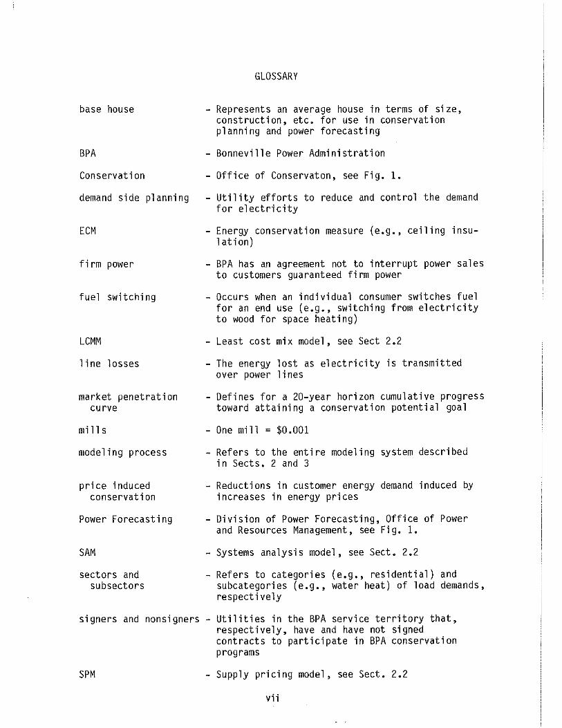
base house - Represents an average house in terms of size, construction, etc. for use in conservation planning and power forecasting
BPA -Bonneville Power Administration
Conservation - Office of Conservaton, see Fig. 1.
demand side planning - Utility efforts to reduce and control the demand for electricity
ECM Energy conservation measure (e.g., ceiling insulation)
firm power - BPA has an agreement not to interrupt power sales to customers guaranteed firm power
fuel switching -Occurs when an individual consumer switches fuel for an end use (e.g., switching from electricity to wood for space heating)
LCMM - Least cost mix model, see Sect 2.2
1 ine losses - The energy lost as electricity is transmitted over power lines
market penetration - Defines for a 20-year horizon cumulative progress curve toward attaining a conservation potential goal
mills -One mill = $0.001
modeling process - Refers to the entire modeling system described in Sects. 2 and 3
price induced - Reductions in customer energy demand induced by conservation increases in energy prices
Power Forecasting - Division of Power Forecasting, Office of Power and Resources Management, see Fig. 1.
SAM -Systems analysis model, see Sect. 2.2
sectors and subsectors
-Refers to categories (e.g., residential) and subcategories (e.g., water heat) of load demands, respectively
signers and nonsigners - Utilities in the BPA service territory that, respectively, have and have not signed contracts to participate in BPA conservation programs
SPM Supply pricing model, see Sect. 2.2
vii

supply curve - Represents conservation available for one sector at one average cost per unit of energy saved over a 20-year period
take back - When customers change energy demands after participating in a conservation program
technical efficiency - Used in load forecasting models to represent curves relationships between capital cost and energy
efficiency for appliances and measures
thermal integrity -The ability of a building to retain internal heat
utilization elasticity - Change in the amount of use of an appliance induced by a change in the operating cost of using the appliance
viii

SUMMARY
Utilities in the United States are attempting to improve their analytic capabilities, especially by integrating models of electricity supply and demand. This report shows how the Bonneville Power Administration (BPA) has done an effective job in this area. Descriptions of conservation forecasting, power forecasting, and resource acquisition models are provided.
Integrating models of supply and demand is a complicated and challenging task. Questions arise over the conceptual validity of individual models, the appropriateness of model interaction, and the quality of data to support mode 1 deve 1 opment. Thus, as a second goa 1 , this report suggests areas of future work that could improve the BPA conservation modeling process and similar processes at other utilities.
To summarize, our analysis revealed no inconsistencies or inappropriate uses of conservation data. This conclusion is not surprising considering how closely the highly competent BPA staff works together. Although the documentation could have been more detailed, it is unlikely that major inconsistencies or inappropriate uses of conservation data exist within the modeling process. The synergism between the staff appears to result in a process that performs as expected.
Based on documentation of the process, we suggest possible areas of future work. For example, modeling of price induced conservation, take back behavior, and conservation technical potentials benefit from additional research. Other suggested work includes incorporating administrative costs explicitly in the process, improving the representation of consumer decision making, and explicitly representing non-BPA conservation costs, uncertainty, and conservation programs.
The conclusion of the report is a discussion of the importance and difficulty of implementing each improvement. Each is classified as having an immediate or deferrable benefit, and each is categorized as moderately or highly difficult to implement. The most attractive improvements (i.e. the immediately beneficial, moderately difficult ones) include developing BPA-specific market penetration rates and representing non-BPA conservation costs in the process.
This report is an expanded version of one completed for BPA (Tonn, Holub, and Hilliard, 1985.) The former report primarily focuses on documenting the conservation modeling process. This report includes views on several areas of possible future work (Sects. 6, 7, 8 and App. A). Because the additional material cannot be discussed without a firm understanding of the modeling process, the previous report is reproduced herein.
ix

INTRODUCTION
Electricity demand forecasting and resource planning has changed
considerably in the past two decades. The 1960s were characterized by
steadily increasing electricity demands and increasing returns to scale
for power generation. Given stable and low energy prices, utilities
could plan to meet new load demands with new generation facilities. The
1970s were characterized by steep energy price increases and uncertain
energy supply availability. The emergence of environmental concerns
associated with electricity generation increased generation costs and
increased construction costs for nuclear power plants. Carried into the
1980s have been efforts to overcome the problems that arose in the
1970s. Specifically, much attention has focused on demand side planning
and on acquiring conservation as a power resource. As a consequence,
many utilities use sophisticated power forecasting models and other
complicated quantitative methodologies to determine cost efficient
capital and conservation investments required to meet load demands.
The Bonneville Power Administration (BPA) has developed a set of
sophisticated mathematical models to assist conservation program
planning, power forecasting, power resource acquisition, and rate
setting. The models are integrated into an analytical policy process,
where outputs of some models act as inputs to others and a continuous
process is formed. For example, modeling electricity prices requires as
an input the costs associated with operating BPA's power system;
modeling what power resources to acquire (e.g., hydro, coal, nuclear,
conservation) and their costs requires forecasts of power demands; and
power forecasting requires inputs concerning future electricity prices.
2
The BPA modeling process addresses the dynamics inherent in power
supply planning and demand analysis. The details encompassed in the
models and the complexity of the process are impressive. An invaluable
benefit of BPA's modeling efforts is a system which represents hundreds,
if not thousands, of characteristics that define the BPA power supply
and demand system. A very real cost of this system, however, is that
modeling groups such as the Office of Conservation have to invest more
and more time to stay abreast of system changes and to understand how
such changes affect their role within the larger modeling process. As
the modeling process becomes more complex, each modeling group has more
difficulty understanding the big picture and keeping track of details
(e.g., are other modeling groups using a particular group's data outputs
appropriately?).
This report draws on work performed by the ORNL for BPA to document
conservation data flows throughout the BPA modeling process, to evaluate
the consistency and appropriateness of the use of conservation data, and
to suggest improvements in the model process with respect to representing
and utilizing conservation data.* Conservation data flows are documented
for each sector- residential, commercial, irrigation, and industrial -
and for each major modeling area- conservation supply curves, heat loss
methodology, power forecasting, resource acquisition, and rates. Data
collected for this report come from interviews conducted with BPA staff
between September 1984 and March 1985. Thus, this report presents a
snapshot of the modeling process, which is continually evolving.
*ronn, Holub and Hilliard (1985) contains the research sponsored by BPA. This report includes suggestions for improving the conservation analysis process.

3
Section 2 describes in general terms the BPA modeling process and
introduces six model areas - conservation supply curves, heat loss
methodologies, power forecasting models, the Least Cost Mix Model, the
Systems Analysis Model, and the Supply Pricing Model. In addition to
stating the purpose of each model, each model's conservation data needs
and products are generally characterized and how each model interacts
with the other models is described.
Section 3 explores in-depth each link in the model process and
documents the conservation data transfers and instances where data
transfers are inadequate or nonexistent. This section is the technical
heart of the report since the final six sections and the appendices use
the information presented in this section as the basis for discussions
concerning modeling process issues and the development of recommendations.
Section 4 investigates the interaction among conservation models
and power forecasting models and the data flows within the conservation
program planning process. Three general issues dominate the discussion:
how the process characterizes price induced conservation, fuel switch
ing, and take back effects; how the process deals with issues concerning
conservation technical potential; and how the conservation planning
process accounts for future program activity in the supply curves.
The fifth section addresses conservation data flows among the
various models. In general, this section highlights the need for conser
vation data that is more specific and mentions the benefits of expli
citly representing administrative costs, developing BPA conservation
costs to complement regional conservation costs, and specifying conser
vation savings with respect to seasonal and peak loads.

4
Section 6 focuses on modeling consumer conservation behavior. This
section suggests that the Office of Conservation and the Division of
Power Forecasting coordinate work with respect to characterizing how
electricity consumers (e.g., households) make energy-related decisions.
We highlight opportunities for incorporating decision models in
conservation program planning and discuss possible difficulties.
The next two sections present a more holistic view of the conser
vation planning process. Section 7 discusses two conservation resource
planning issues. One pertains to representing conservation potential in
the Least Cost Mix Model by supply curves. The second addresses incor
poration of uncertainty about conservation resources into the modeling
process.
Section 8 steps back even further to present issues concerning con
servation planning policy that have a future orientation: developing
conservation-specific planning scenarios and planning with respect to
foregone opportunities.
Section 9 presents priorities of recommendations for possible future
work discussed in the previous five sections. Specifically, we classify
issues into four groups - issues that appear moderately difficult to
implement but could yield substantial potential benefits to the conser
vation planning process, very difficult to implement with substantial
benefits, moderately difficult to implement with deferrable benefits,
and very difficult to implement with deferrable benefits.
The two appendices focus on topics too technical for the main body
of this report. Appendix A presents a formulation for a resource
allocation model to represent actual conservation programs instead of

5
the current supply curve formulation. Appendix B discusses the
characteristics of base houses (i.e., representative or reference
houses) in power forecasting and conservation planning.

7
2. OVERVIEW OF BONNEVILLE POWER ADMINISTRATION CONSERVATION/ LOAD/RESOURCE MODELING PROCESS
2.1. INTRODUCTION
This section provides an overview of BPA's modeling process. The
overall goal of the process is to provide the technical information
required by policy makers to manage the BPA system to meet demands for
power by consumers in the Pacific Northwest at minimal cost. The
interactions of the models are complex and must be understood in signi-
ficant detail before proceeding to the documentation of the data flows
in the modeling process (Sect. 3).
2.2. BPA CONSERVATION/LOAD/RESOURCE MODELS
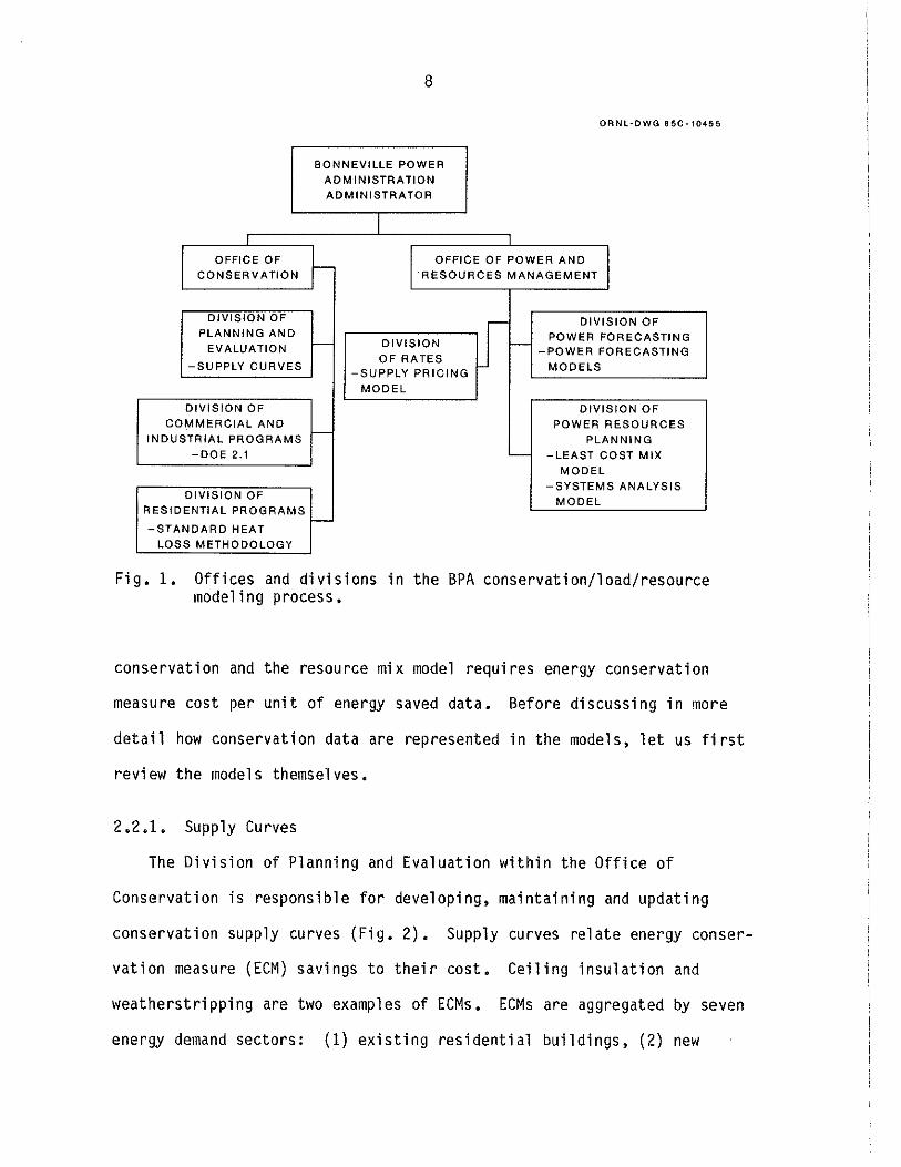
The models are developed, maintained and exercised in two offices
and six divisions within BPA (Fig. 1). The Office of Conservation is
responsible for estimating region-wide conservation technical potential,
designing conservation programs to acquire conservation resources, and
estimating the cost and market penetration of the programs. It employs
models which relate conservation savings to cost (supply curves) and
which calculate expected energy savings due to installation of energy
conservation measures in buildings (heat loss methodologies).
The Office of Power and Resources Management is responsible for
forecasting future power demands (load forecasting models), acquiring
resources at the lowest cost to meet the forecasted demands (Least Cost
Mix and System Analysis Models), and exploring rate structures that
would supply revenue for the BPA operating system (Supply Pricing
Model). These models incorporate conservation data in many ways. For
example, the forecasting models require data on historical levels of
8
ORNL·DWG 85C·10455
BONNEVILLE POWER ADMINISTRATION ADMINISTRATOR
I
OFFICE OF r- OFFICE OF POWER AND CONSERVATION RESOURCES MANAGEMENT
DIVISION OF - DIVISION OF PLANNING AND POWER FORECASTING
EVALUATION - DIVISION r- -POWER FORECASTING -SUPPLY CURVES
OF RATES MODELS -SUPPLY PRICING
MODEL
DIVISION OF DIVISION OF COMMERCIAL AND POWER RESOURCES -INDUSTRIAL PROGRAMS PLANNING
-DOE 2.1 - -LEAST COST MIX MODEL
-SYSTEMS ANALYSIS DIVISION OF
MODEL RESIDENTIAL PROGRAMS
-STANDARD HEAT I-LOSS METHODOLOGY
Fig. 1. Offices and divisions in the BPA conservation/load/resource modeling process.
conservation and the resource mix model requires energy conservation
measure cost per unit of energy saved data. Before discussing in more
detail how conservation data are represented in the models, let us first
review the models themselves.
2.2.1. Supply Curves
The Division of Planning and Evaluation within the Office of
Conservation is responsible for developing, maintaining and updating
conservation supply curves (Fig. 2). Supply curves relate energy conser
vation measure (ECM) savings to their cost. Ceiling insulation and
weatherstripping are two examples of ECMs. ECMs are aggregated by seven
energy demand sectors: (1) existing residential buildings, (2) new

ANNUAL
CONSERVATION
ENERGY
SAVINGS (kWh/yr)
0
9
ORNL-DWG 8SC-10454A
ESTIMATED MAXIMUM ENERGY CONSERVATION --------------- :::;,..o---1
POTENTIAL
5 10 15 20
YEAR IN PLANNING HORIZON
Fig. 2 Example of BPA conservation supply curve
residential, which includes new residential buildings, home appliances,
and water heaters, (3} existing commercial buildings, (4} new commercial
buildings, (5} irrigation, (6} direct service industries (DS!s} ,*and
(7) nondirect service industries.
Energy conservation measure savings are grouped into six cost cate
gories for each sector except for the DS!s, which are grouped into two
cost categories. The six cost categories are 0-15, 15-20, 20-25, 25-30,
30-35, and 35+ mills/kWh and the two cost categories for DS!s are 0-20
and 20+ mills/kWh. Energy conservation measure cost data exist for the
existing residential sector and the water heat subsector of the new
*Direct service industries (DSI} are large industrial customers that sign separate contracts with BPA to acquire power at negotiated rates and loads.

10
residential sector and, based on this data, costs per unit energy saved
per measure are objectively distributed over the cost categories. In
the other sectors and subsectors, costs are judgmentally distributed
over the cost categories.
The supply curves are constructed in the following way. First,
total potential energy savings for each sector and cost category are
estimated for a 20-year planning horizon. That is, it is determined on
an annual basis how much energy could be saved from conservation in the
next twenty years. Data which enter these calculations come from heat
loss methodologies (Sect. 2.2.2), engineering reports, conservation
program evaluation results, and load forecasting models (Sect. 2.3).
Second, energy savings are distributed over the 20-year planning
horizon using market penetration ramps. The ramps, first de vel oped by
Applied Management Sciences (1983), generally resembleS-curves, where
penetration is slow in the near-term, accelerates in the mid-term, and
slows again in the far-term (Sect. 3.2, Fig. 5). A ramp consists of 20
numbers between.O.O and 1.0 which indicate the percentage of the poten
tial conservation expected to be acquired in that year. For programs
that have been operating for some time, the ramps are adjusted more
toward the up-slope of the S-curve (i.e., the ramps are moved left).
This is the case with the "existing residential'' supply curve. Other
ramps are adjusted rightward in expectation of slower initial penetra
tion (e.g., home appliance and home water heater subsector curves). In
general, though, all the ramps possess the S-curve shape.
An example will help explain the nature of supply curves. The
existing residential 0-15 mill/kWh supply curve was developed from the

11
20-year aggregated annual potential savings due to installation in
existing residential buildings of several measures (e.g., R-19 ceiling
insulation) that cost between 0-15 mills/kWh. The 20-year planning
horizon potential was distributed according to a market penetration
ramp. The result is a supply curve consisting of 20 numbers which
represent cumulative energy savings for each year in the planning horizon.
2.2.2. Heat Loss Models
The Office of Conservation uses two heat loss methodologies to help
estimate conservation potential in the Pacific Northwest. The Division
of Residential Programs maintains the Standard Heat Loss Methodology
(SHLM). It is an engineering simulation of heat losses from residential
buildings and was developed using guidelines from the American Society of
Heating, Refrigerating, and Air Conditioning Engineers. The Division of
Commercial and Industrial Programs uses DOE 2.1, developed by the U.S.
Department of Energy, to simulate heat losses from commercial buildings.
The models' inputs include: weather; the building structure (e.g.,
wood frame single-story house); heating, cooling, and ventilation
equipment; and the number and behavior of the occupants. The outputs
include annual energy consumption for average residential and commercial
buildings and estimates of energy savings potential due to installation
of energy conservation measures.
2.2.3. Load Forecasting Models
The Division of Power Forecasting in the Office of Power and
Resources Management develops, maintains, and up-dates power forecasting
models. The models may be classified by sector and by their forecast
horizons.
12
The Mid-Term Energy Demand Forecasting Model (BPA, 1984) forecasts
sector-unspecific monthly electricity demand for each state in the
Pacific Northwest for a seven- to ten-year period. This is an econo
metric model, able to incorporate short-term variables such as weather,
business cycles, and economic fluctuations.
The Oak Ridge National Laboratory Residential Reference House Energy
Demand Model (RRHED) (Hamblin, 1985) is used to forecast long-term
residential electricity demand. A 20-year forecast is made for
publicly- and investor-owned utilities. The model is an engineering/
econometric model that incorporates technology curves, household effi
ciency choices and household fuel choices. It forecasts energy
demand for nine end uses (space heating, air conditioning, water
heating, cooking, drying, refrigerators, freezers, lighting and other),
four fuels (electricity, gas, oil and other) and three house types
(single family, multi-family, mobile home). More details of this model
are discussed later (Sect. 3, Appendix B).
The Bonneville Power Administration Commercial Energy Demand Model
forecasts annual commercial energy demand for 20 years for 12 different
building types (e.g., offices, restaurants). The model is an engineering
model that forecasts demand based on forecasted changes in square footage
for each of the building types.
Econometric models are used to forecast long-term irrigation,
non-DSI industrial and OS! aluminum energy demands. Econometric and
subjective methods are used to forecast non-aluminum OS! energy demands.
13
2.2.4. Least Cost Mix Model
The Division of Power Resources Planning in the Office of Power and
Resources Management oversees two models. One is the Least Cost Mix
Model (LCMM}. It determines the least cost mix of power resources to
meet forecasted power demands, It takes existing resources as given and
accepts as inputs supply curves for new power resources (hydro, coal,
nuclear and conservation) and demand forecasts. Resource costs over
time are adjusted upward for inflation (6% per year) and downward for
the time value of money (3% per year) to allow consistent comparison of
costs across resources (BPA, 1984b}. The model employs linear program
ming to find the least cost mix over a twenty year planning horizon.
The model outputs power to be acquired for each new resource for each
year and the acquisition costs.
2.2.5 Systems Analysis Model
The Division of Power Resources Planning also maintains the Systems
Analysis Model (SAM}. The model "performs a probabilistic simulation
of the region's power system, using existing and planned resources to
meet forecasted loads season by season, month by month, and hour by
hour. SAM has the capability to evaluate the impacts for the following
major components of the region's power system: policies of regional
planning and operation, uncertainties of loads and resources, nonpower
constraints on the hydro system, transactions outside the region,
revenue requirements among sponsors, and cost of operations" (BPA, 1984c}.
The region's power sources modeled include hydro, nuclear, and coal.
Conservation is not currently modeled. Uncertainty is handled in a pro
babilistic fashion with respect to regional loads (e.g., by varying
14
weather and economic conditions) and hydro resources (e.g., by varying
water flows into reservoirs). All data inputs come from the LCMM.
SAM's output is used primarily for policy analysis and does not flow
into other models.
2.2.6. Supply Pricing Model
The Division of Rates maintains the Supply Pricing Model (SPM).
This model simulates the BPA rate setting process and the rate setting
process of the region's retail electric utilities. The model can also
produce "1 ong-term projections of annua 1 rates and mid-term projections
of monthly retail rates. Wholesale rates for priority firm power,
industrial firm power, new resource firm power, and nonfirm energy, plus
the fully allocated cost of surplus firm power are estimated by the SPM.
It also produces retail rates for the residential, commercial, and
industrial sectors of both investor-owned (private) and publicly-owned
(public) utilities. Finally, it produces monthly retail rates for
nongenerating public utilities by state and for generating public utili
ties at the regional level" (BPA, 1984a, p. 2). It receives system cost
data from the LCMM and load forecast data from the forecasting models,
and its outputs, electricity prices, are used by the forecasting models
(Sect. 2.3).
2.3 MDDEL INTERACTION PATTERNS IN THE BPA MODELING PROCESS
This subsection provides a general overview of how the models
described above interact with each other (Fig. 3). The eleven steps of
the modeling process are carried out for several load growth scenarios
and conservation resource levels. For example, power forecasts are
made under three scenarios related to the region's economic and load

15
growth (high, medium and low). Also, the process is run using three
conservation resource levels - F1, F2 and F3. The F1 level refers to
conservation that has been achieved through the last complete fiscal
year. The F2 level refers to F1 conservation plus estimates of conser-
vation due to already budgeted programs (2 years in the future), and
estimates of conservation from minimum viable conservation programs that
* BPA is contractually committed to offer. The F3 level refers to F2
conservation plus conservation savings that can be acquired by the Least
OANL-DWG 85C-7190A
HEAT LOSS METHODOLOGIES
AND FORECASTING DATA BASES
~--------------~
HEAT LOSS METHODOLOGIES
AND CONSERVATION
DATA BASES
N z
<no wu>_<(
a: a: a.w ~t:: ~CJ >-z
""
TECHNICAL INPUT 2A 10
LOAD FORECAST
MODELS
CONSERVATION PROGRAM TARGETS
HISTORICAL CONSERVATION SAVINGS 1
DEMOGRAPHIC 4
TECHNICAL INPUT 5
SUPPLY CURVES AND
CONSERVATION PROGRAMS
1 l!: '>"'~,~:;;;;,"1-A,_:S:_:~:_:~..:=..::~.:..:...:S 6"-...J
g: ~~g {LCMM) CONSERVATION RESOURCE 9 ...J zwu;: ACQUISITIONS
~<(!:0.. '
SUU:PPLY <c"-"~'J-'0~'<- 1 "'> ,--S-Y-ST_E_M_S--,
PRICING ANALYSIS MODEL MODEL (SPM) (SAM)
Fig. 3. Overview of BPA conservation/load/resource modeling process. The numbers 1 through 11 refer to the sequence of interactions among the elements of the process.
*operating a conservation program at the lowest possible level (i.e., to maintain organizational experience in the program's operation) is known as the program's minimum viable level. The programs are run at minimum viable levels to build BPA's capability of flexibly and efficiently meeting future power resource demands.

16
Cost Mix Model (i.e., over and above minimum viable program levels).
The interactions illustrated in Fig. 3 are run under F2 and F3, and F1
and F3 conservation levels, although the following discussion assumes
the process is being run under F3 conservation levels.
* Interactions among the models are broken into eleven steps. The
first interaction (historical conservation savings - 1) is between the
load forecasting models and the Office of Conservation. Conservation
sends to the power forecasting models fiscal year data for years 1981 to
1983 on the number of units (e.g., residences) treated by the conser-
vation programs, the savings per unit in kWh/year, energy conservation
measure life, and end-of-year and mid-year annual and cumulative savings
in average MW. These estimates are provided for public and investor
owned utilities and by consuming sector (residential, commercial, DSI,
non-DSI industrial and irrigation).** The estimates of historical con
servation (F1) are used to update data in the models that relate to
stock and appliance energy efficiency.
Detail varies within consuming sectors. For the residential sector,
data are provided by housing type (e.g., single family, multi-family and
mobile home) and program (e.g., weatherization, water heater wrap,
shower flow restrictor). For the commercial sector, data are provided
by program (e.g., water heater wrap, shower flow restrictor, lighting,
* In addition, individuals responsible for working in each of the modeling areas regularly communicate with each other on an informal basis. Such communication has not been documented here. This discussion does not capture in full detail all the activities that comprise the process. This is especially true of the models' characterization of resources other than conservation.
**Information provided with respect to this interaction is drawn from a memo prepared by Forman (1984).
17
and institutional build1ngs). Savings due to BPA's street and area
lighting program are also included in the commercial totals. DSI and
industrial data are not detailed by program. Irrigation data are pro
vided for center pivot and other retrofit programs.
The second interaction (initial prices and iteration -2) is between
the forecasting models and the Supply Pricing Model. The SPM takes the
F3 load forecasts developed during the preceding modeling process cycle
(last year, for example) and produces a set of seed (initial) prices
needed to meet the revenue requirements for the system, as dictated by
the power forecast. These seed prices are passed to the power fore
casting models and new forecasts are made. The new forecasts are input
into the SPM and new rates are calculated. This process continues until
there is less than a 1% change in price and power forecasts (BPA, 1984).
Step (2A) relates to technical data input to the forecasting models.
The third and fourth steps take place simultaneously. The power fore
casts resulting from step (2) are sent in step (3) to the Least Cost Mix
Model. The forecasts are incorporated as a constraint in the LCMM.
The fourth interaction (4) is between the supply curves and Power
Forecasting. Power Forecasting provides data from the forecasting
models to the Office of Conservation needed to calibrate the supply
curves with respect to existing potentials. In the commercial sector,
for example, annual commercial floor space by utility type for 1981
through the current forecast year are provided.
In the residential sector, data are provided on electric appliance
stocks. For water heaters and appliances, occupied housing stock and
electric water heater and appliance saturations are provided for the
year 2000. Occupied stock and electric space heat saturations are pro-
18
vided for multi-family and mobile homes for years 1980 through 1983,
For existing single family houses, 1983 occupied stock, electric space
heat saturation and housing stock retirement rates are provided. For
new single family houses, the annual numbers of new electrically heated
units are provided for the 1980-2000 period. All data are provided by
public and investor-owned utility types (Forman, 1984}.
In the fifth interaction (5}, the supply curves are updated with data
pertaining to the technical potentials for energy conservation in the
various sectors. Curves representing the residential and commercial
sectors are updated with data from the heat loss methodologies, while
the residential sector curves are updated with useful information from
program evaluations (e.g., Hirst et al ., 1985}. Sector-specific data
bases are also used to update the curves (Sect. 3). The data incoming
to the supply curves in interactions four and five are used to update
the supply curves (i.e., adjust upward or downward 20 year horizon con
servation potentials).
After the 38 supply curves are developed, they are represented in a
form usable by the Least Cost Mix Model and sent to the LCMM (6}. Not
shown in Fig. 3 is the transfer of power resource data other than that
associated with conservation.
The seventh area of interaction (7) is an iterative process between
the Least Cost Mix Model and the Systems Analysis Model. SAM explores
in-depth the operation of the Pacific Northwest's power supply system
given resource acquisitions from the LCMM.
Interactions eight and nine are essentially simultaneous. In step
eight (8}, the resource acquisitions chosen by the LCMM are sent to the

19
Supply Pricing Model. These resources always include F3 levels of con-
servation. Especially important are the regional costs over time asso
ciated with the resource acquisition targets. In interaction nine (9),
the conservation resources chosen by the LCMM are sent to the Office of
Conservation so that programs may be designed to meet the targets.* In step ten (10), the Office of Conservation transmits to the power fore
casting models the levels of conservation due to BPA programs that are
expected by sector and utility type for the 20-year planning horizon.
The process concludes with interaction eleven (11) where the power
forecasting models and the Supply Pricing Model again iteratively
interact. In this case, the SPM is given conservation-adjusted load
forecasts (Sect 3) as well as the costs determined by the LCMM.
The eleven step process encompasses data for each of three load
growth scenarios. The discussion above assumes F3 conservation levels. For F2 conservation levels, the LCMM is constrained to choose minimum
viable levels of conservation by setting the cost for the programs equal
to zero in the objective function and conservation resource targets do
not pass through the Office of Conservation before going to the Division
of Power Forecasting. For Fl conservation levels, conservation is not
represented in the LCMM.
*After two iterations of the process shown in Figure 3, conservation resource acquisitions are sent from the LCMM to the Division of Power Forecasting.


21
3. CONSERVATION DATA FLOWS IN THE MODELING PROCESS
3,1 INTRODUCTION
This section is the heart of the report. The detailed descriptions
of the conservation data flows among the five major modeling areas
discussed in the previous section (supply curves, demand models, least
cost mix model, systems analysis model, supply pricing model) serve
many purposes. Most importantly, the conservation data flows are docu
mented. The BPA modeling process has evolved into a highly complex
structure over time and there are significant benefits from documenting
conservation's role in the process and how each model employs conser
vation data.
This exercise also provides the foundation from which to analyze the
process. Are the conservation data flows consistent with the goals of
the process? Do offices and divisions outside the Office of Conservation
use conservation data appropriately and consistently? In what ways
might the process be improved? The following five sections use the
information presented herein to explore these types of questions.
This section is divided into four parts. Each part addresses in
detail the conservation data flows associated with one element of the
larger BPA modeling process shown in Fig. 3, Each of the four subsec
tions contains a figure illustrating magnified detail; the figures
represent data flows within the Office of Conservation, between the
Office of Conservation and Division of Power Forecasting, between
the Office of Conservation and Division of Power Resource, and between
the Office of Conservation and Division of Rates.
22
The discussion on data flows allows for three types of data flows.
Actual data flows are part of the formal BPA modeling process. Implicit
data flows pertain to information (not formal data) exchanged between
modeling groups about conservation data. Nonexistent data flows pertain
to conservation data that could flow and/or has a formal avenue through
which to flow, but did not flow at the time of this analysis.
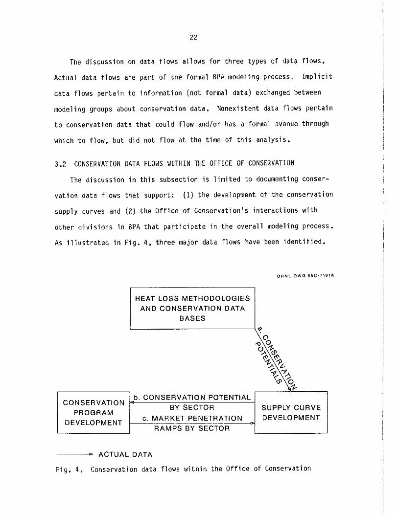
3.2 CONSERVATION DATA FLOWS WITHIN THE OFFICE OF CONSERVATION
The discussion in this subsection is limited to documenting conser-
vation data flows that support: (1) the development of the conservation
supply curves and (2) the Office of Conservation's interactions with
other divisions in BPA that participate in the overall modeling process.
As illustrated in Fig. 4, three major data flows have been identified.
ORNL-OWG 85C-7191A
HEAT LOSS METHODOLOGIES
AND CONSERVATION DATA
BASES
<$? (l
~ 0-t-~~ ~ .p.t..
/ 1' ,.,.A ('<.fl -o
1-
CONSERVATION b. CONSERVATION POTENTIAL
PROGRAM BY SECTOR SUPPLY CURVE
DEVELOPMENT c. MARKET PENETRATION DEVELOPMENT
RAMPS BY SECTOR
ACTUAL DATA
Fig. 4. Conservation data flows within the Office of Conservation
23
Data flow "a" relates to conservation data that flow from the heat
loss methodologies (Sect. 2.2.2) and the conservation data bases into
supply curve development process. Data bases which support the process
include the 1979 and 1983 Pacific Northwest Residential Energy Surveys
(residential sector), the Westat data base (commercial sector), a data
base developed for the industrial sector by Synergic Resources
Corporation (SRC, 1983), and data bases developed for the agricultural
sector by Battelle Pacific Northwest Laboratory and Oregon State
University.
The heat loss methodologies and conservation data bases provide data
on the costs and expected energy savings potential of energy conser
vation measures installed in single family homes, for example. Appendix
B.2 discusses the base houses used to estimate energy savings. Data are
also provided on the potential energy savings and costs for adopting
more efficient energy consuming technologies, such as lighting in the
commercial sector. The data are specified by potential energy saving and
cost per unit of study (e.g., a single family home, square foot of
office building). Conservation potentials are aggregated first by sub
sector, then by sector, to determine maximum technical conservation
potential for a 20-year planning horizon.
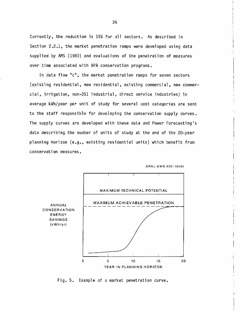
In data flow "b", the maximum technical conservation potentials by
sector and subsector for a 20 year planning horizon are transmitted to
staff responsible for conservation program development. The conser
vation potentials are ramped over the 20 year planning horizon (Fig. 5).
The maximum technical potentials are adjusted downward to represent
expected maximum market penetration of energy conservation measures.
24
Currently, the reduction is 15% for all sectors. As described in
Section 2.2.1, the market penetration ramps were developed using data
supplied by AMS (1983} and evaluations of the penetration of measures
over time associated with BPA conservation programs.
In data flow "c", the market penetration ramps for seven sectors
(existing residential, new residential, existing commercial, new commer-
cial, irrigation, non-DSI industrial, direct service industries) in
average kWh/year per unit of study for several cost categories are sent
to the staff responsible for developing the conservation supply curves.
The supply curves are developed with these data and Power Forecasting's
data describing the number of units of study at the end of the 20-year
planning horizon (e.g., existing residential units) which benefit from
conservation measures.
ANNUAL CONSERVATION
ENERGY SAVINGS (kWh/yr)
ORNL-OWG 85C-10454
I
MAXIMUM TECHNICAL POTENTIAL
MAXIMUM ACHIEVABLE PENETRATION f--------------- --__,--~
I I I
0 5 10 15 20
YEAR IN PLANNING HORIZON
Fig. 5. Example of a market penetration curve.

25
3.3 OFFICE OF CONSERVATION-DIVISION OF POWER FORECASTING DATA FLOWS
The data flows between the Office of Conservation and the Division
of Power Forecasting (Fig. 6) appear to be the most complex and most
numerous of the inter-office interactions. Of the six data flows
described, three are actual, one is implicit and two are nonexistent.
Data flow "a'', from the Office of Conservation to the Divison of
Power Forecasting, concerns historical energy conservation savings due to
program activities (i.e., not including price induced conservation) up
to the present (Forman, 1984). In other words, the data represent, for
fiscal years 1982 and 1983, the number of treated units (e.g.,
weatherized single family houses), the savings per unit in kWh/year,
energy conservation measure lives, and end-of-year and mid-year annual
and cumulative savings in average MW. The data are provided by sector
for public and investor-owned utility types.
Additional detail varies within the consuming sectors. For the
residential sector, the Office of Conservation provides data by housing
type and by program type. For the commercial sector, data are provided
only by program type. Savings due to BPA's street and area lighting
program are also included in the commercial totals. Agricultural sector
data are provided for the center pivot irrigation systems and other
programs. Industrial sector data are not broken down into subsectors.
An important element of the evaluation exercise performed for BPA in
CON-179 was to determine how offices other than Conservation use conser
vation data. The next few paragraphs detail how the Division of Power
Forecasting uses estimates of past program saving.
In the commercial, industrial, and irrigation sectors, programmatic
savings (in average MW) are subtracted from the demand forecasts (see

26
OFFICE OF POWER AND RESOURCES
MANAGEMENT DIVISION OF
POWER FORCASTING
a. PAST PROGRAM SAVINGS DEMAND MODELS:
RESIDENTIAL ~PRICE INDUCED SAVINGS., ---------COMMERCIAL c. DEMOGRAPHIC DATA
MID-TERM d. FUEL SWITCHING :..::·------------------- _. IRRIGATION e. TAKE BACK BEHAVIOR :..::·----------------- -- .... NON-DSI
INDUSTRIAL f. FUTURE CONSERVATION
PROGRAM SAVINGS DSI ALUMINUM
DSI NON-ALUMINUM
ACTUAL DATA -- _..,. IMPLICIT DATA _____ ..,.. NON-EXISTENT DATA
ORNL·OWG 65C·7192A
OFFICE OF CONSERVATION
CONSERVATION
PROGRAM
DEVELOPMENT
SUPPLY CURVES
DEVELOPMENT
Fig. 6. Office of Conservation - Division of Power Forecasting conservation data flows.
Sect. 2.2.3 for model definitions). In the commercial sector, program-
matic saving estimates are reduced by 20 percent by Power Forecasting
(in both the commercial and street lighting models) to correct for
double counting of price induced efficiency gains projected by the end-
* use mode 1 s and to account for take back effects.
The residential sector use of the programmatic savings is complex.
The residential demand model uses number of units (e.g., houses
weatherized, water heaters wrapped) by housing type provided by the
Office of Conservation. Savings per housing unit are translated into
*Take back effects refer to changes in customer energy demand after participation in a BPA conservation program.
27
energy indices that are also direct model inputs. These indices are the
ratios of appliance energy use (or dwelling thermal integrity)* in a
treated housing unit to the appliance energy use (or dwelling thermal
integrity) in a stock average housing unit in the base year of the
model. The stock average housing unit refers to a theoretical house
which portrays the average characteristics of all the houses in the
Pacific Northwest existing during the year 1979. (See Appendix B for
more detail on residential stock average houses.)
For example, in the public utility group, base year single family
electric water heat use is 4515 kWh/year. The Office of Conservation
projects savings of 435 kWh/year for water heater wraps in 1982 and
1983. This yields an energy index of (4515-435)/4515=.904 for wrapped
water heaters. A similar calculation is made for weatherization, but
here the index represents the dwelling shell thermal integrity indices
after weatherization relative to a base year value of 1.0 (Appendix B).
The residential model uses the number of units and the index values
associated with the conservation programs in the following steps to
reduce the estimates of average electricity use. First, the housing
stock eligible for a particular conservation program is calculated based
on input data (year and quantity of stock eligible for the conservation
program) and equipment (or dwelling) retirements. Then the actual
number of units treated by conservation programs are removed from the
program eligible stock group in the base year and added to the retro
fitted (or treated) group.
*Thermal integrity refers to how well a house retains internal heat.

28
As a third step, the residential model simulates some usage take
back (or changes in energy use patterns induced by retrofits) for the
treated houses by increasing the end-use usage (or utilization)* fac
tor, since some householders are expected to "consume" part of their
energy savings, all other things being equal. Changes in energy con
suming equipment utilization are restricted to remain between 90% and
110% of the prior period energy use and are determined as a function of
preprogram energy use, operation costs, and changes in household income.
Finally, the measure lifetimes developed jointly by the Office of
Conservation and the Division of Power Forecasting are used to retire
retrofitted appliances or shell improvements at the end of their pro
jected lives. Housing units weatherized are not candidates for demoli
tion within the residential model until their weatherization measures
reach the end of their projected lifetimes.
Data flow "b" (Fig. 6} relates to implicit information exchanged be
tween the Office of Conservation and the Division of Power Forecasting
concerning price induced conservation in the 20 year planning horizon.
Because BPA does not wish to finance conservation measures that electri
city consumers would have taken in the absence of BPA programs, accurate
identification of price induced conservation behavior is important. One
source of information comes from the load forecasting models, which con
sider market driven conservation within their equipment and shell effi-
*Price effects are also simulated.
29
ciency choice mechanisms.* At this point in the process, the two groups
agree on the extent of price induced conservation in order to adjust the
supply curves' conservation potentials downwards. Currently, 20% is
subtracted off the 20 year planning horizon maximum market penetration
conservation potential in the commercial sector and residential water
heater and appliance subsectors. Twenty percent is also subtracted from
the irrigation and non-DSI sectors. All other potentials remain
unchanged.
The 20% figure used in the commercial sector was judged reasonable
using the following assumptions. In all commercial conservation
programs except institutional buildings and street lighting, consumers
are assumed to share costs with BPA equivalent to a two year payback.
Two years was chosen because it appeared consistent with the payback
periods of other commercial investments. In the buildings and lighting
programs, payback was assumed to be one and less than one year, respec-
tively. Aggregating these assumptions in the commercial sector yields
an estimate of 20% price induced. A similar exercise is associated with
the 20% figure in the irrigation and non-DSI sectors.
*For example, the residential model incorporates price induced behavior in three ways. One, energy prices affect the life cycle costs associated with replacing worn out appliances in existing residences and choosing shell and appliance efficiencies. Higher prices would lead to choices of more efficient equipment and shells, all else being equal. Two, energy prices affect the choice of fuel types. Three, price changes also affect appliance utilization. Implicit discount rates are estimated by building type, income, and end-use using a discrete choice methodology (Hamblin, 1985). The commercial model also incorporates prices in its building equipment and shell life cycle cost calculations and its utilization response.
30
The Office of Conservation and the Division of Power Forecasting
work together to determine no cost/low cost measures in the residential
sector. No formal criteria are used to make these determinations,
partly because BPA conservation programs cover some low cost measures
(e.g,, shower flow restrictors). A small number of measures related to
water heating are assumed to be price induced and the 20-year penetra
tion potential is reduced 20% accordingly. No price induced conser
vation is assumed to take place with respect to home building shell
efficiency because of high retrofit costs.
Data flow "c" pertains to demographic data transferred from the
energy demand models to be used in developing the supply curves. These
data are fully described in Section 2.2.1.
Data flows "d" and "e" are nonexistent and pertain to fuel switching
and take back behavior, respectively. Fuel switching refers to con
sumers changing the fuel for major energy end uses (e.g., space heating)
and is modeled in both the residential and commercial demand models. In
the residential model, a discrete choice (nested logit) model describes
how households choose between 81 space heating fuel/water heating fuel
combinations for their new homes (Hamblin, 1985). Many fewer options
are available in the commercial model and the choices are made by mini
mizing life cycle costs (Jackson and Lann, 1983), Thus, these two
models address fuel switching behavior. No data flow back to the Office
of Conservation about the extent of fuel switching over time in the
residential sector that affect construction of the supply curves.
Take back behavior refers to changes in energy use related to par-
t i ci pat ion in a conservation program. The resident i a 1 and commercia 1
models include take back behavior. As mentioned above, in the residential

31
model the take back elasticity is restricted to remain between 0.9 and
1.1. The elasticity in the commercial sector is even more restricted,*
because consumer comfort is a high priority in this sector. No take
back data affect the construction of the supply curves.
The sixth data flow, "f", pertains to conservation program savings
estimates sent by the Office of Conservation to the Division of Power
Forecasting developed as a response to conservation targets set by the
Least Cost Mix Model (Sect. 3.4). (After two iterations of the
modeling process illustrated in Fig. 3, these data flow directly to
Power Forecasting from the LCMM.) The data are provided in average kWh
per year for 20 years by sector and utility type for use in the long run
models. The data are provided in average MW for five years by utility
for use in the mid-term model. These programmatic conservation esti
mates are subtracted from the load forecasts before they are sent to the
Supply Pricing Model (see step 11, Fig. 3).
The representation of data flow "f" in Fig. 6 does not indicate how
Conservation analyzes and transforms the LCMM conservation resource
targets. Conservation utilizes a spreadsheet computer program known as
the Program Mix Model (PMM) (Gordon, 1983) to distribute targets across
on-going and future conservation programs over the 20-year planning
horizon. Savings per program (Avg. MW) and costs per program per year
are estimated for the three load demand scenarios. Then sensitivity
analysis is performed with respect to these estimates. New supply
curves are created with the first two years of the planning period removed.
The supply curve penetration ramps are also recalibrated to better fit
*Personal communication with Dan Hamblin.
32
with observed market penetrations. The new supply curves are developed
under a number of scenarios (e.g. load demand growth, nuclear power
plant development) and are sent to the LCMM. Given the results of this
sensitivity analysis, new conservation targets are developed and run
through the Program Mix Model again. Conservation costs and savings are
recalculated for the three load growth scenarios and sent to Power
Forecasting. These numbers represent the F3 conservation forecast.
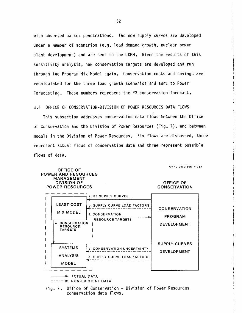
3.4 OFFICE OF CONSERVATION-DIVISION OF POWER RESOURCES DATA FLOWS
This subsection addresses conservation data flows between the Office
of Conservation and the Division of Power Resources (Fig. 7), and between
models in the Division of Power Resources. Six flows are discussed, three
represent actual flows of conservation data and three represent possible
flows of data.
OFFICE OF POWER AND RESOURCES
MANAGEMENT DIVISION OF
POWER RESOURCES
------· a. 38 SUPPLY CURVES
LEAST COST ,:_-SUPPLY CURVE LOAD FACTORS ------------------------
MIX MODEL f. CONSERVATION
RESOURCE TARGETS e. CONSERVATION I RESOURCE
TARGETS I I I
SYSTEMS .. c_- CONSERVATION UNCERTAINTY ------------------------ANALYSIS .. t SUPPLY CURVE LOAD FACTORS
----------------------MODEL
I ______ ___, l _
ACTUAL DATA -----+ NON-EXISTENT DATA
ORNL-OWG 85C-7193A
OFFICE OF CONSERVATION
CONSERVATION
PROGRAM
DEVELOPMENT
SUPPLY CURVES
DEVELOPMENT
Fig. 7. Office of Conservation- Division of Power Resources conservation data flows.
33
Data flow "a" pertains to the transfer of the 38 supply curves
(Sect. 2.2.1) from the Office of Conservation to the Division of Power
Resources for input into the Least Cost Mix Model. The supply curve
energy savings potentials are increased by 6.7% for all sectors to
account for transmission line losses.
Data flow "b" indicates that the supply curves could be specified by
their load characteristics. Specifically, the LCMM can input conser
vation resource factors by three seasons and three times during the day.
Currently, conservation is assumed to have no time-of-day variation.
With respect to seasonal variation, the Office of Conservation provides
monthly load estimates which the Divison of Power Resources translates
into seasonal load factors using Conservation's monthly savings factors.
This particular data flow is characterized as nonexistent because the
Division of Power Resources performs some of the necessary calculations.
Future work could aim at formalizing this data flow element.
Data flow "c" pertains to data which could flow from the Office of
Conservation to the Systems Analysis Model concerning the uncertainty
inherent in the conservation program estimates. Specifically, the SAM
can accept a five-point distribution which relates levels of conservation
resource performance and penetration to probabilities of attaining the
levels. This capability is currently not used.
Data flow "d" pertains to data concerning hourly effects upon load
of the acquisition of conservation resources which could flow from
Conservation to SAM. Monthly estimates are not adequate to estimate
hourly loads. The Division of Power Resources developed a computer
program to weight conservation acquisitions in an hourly manner, but the
process could be improved if the Office of Conservation assumed respon-
34
sibility for these calculations or used another model to prepare the
estimates.* Thus, the process could be improved if data on uncertainty
were provided to the SAM and if hourly load effects of conservation were
calculated within the Office of Conservation.
Data flow "e" pertains to the flow of information between the LCMM
and the SAM relating to conservation resources selected over time by the
LCMM. Regional average MW conservation savings by month for the 20-year
period as chosen by the LCMM are sent to the SAM and these energy
savings are subtracted from system loads input into the Systems Analysis
Model. Therefore, no conservation data are directly represented in the
SAM.
Data flow "f" contains the final conservation resource targets set by
the LCMM (regional average MW by month for 20 years by sector). The
Office of Conservation uses these targets, especially targets in the
near term, to help define their conservation programs. The Office of
Conservation decreases these targets by 6.7% to account for transmission
line losses, and increases these targets by specific amounts to account
for price induced conservation.
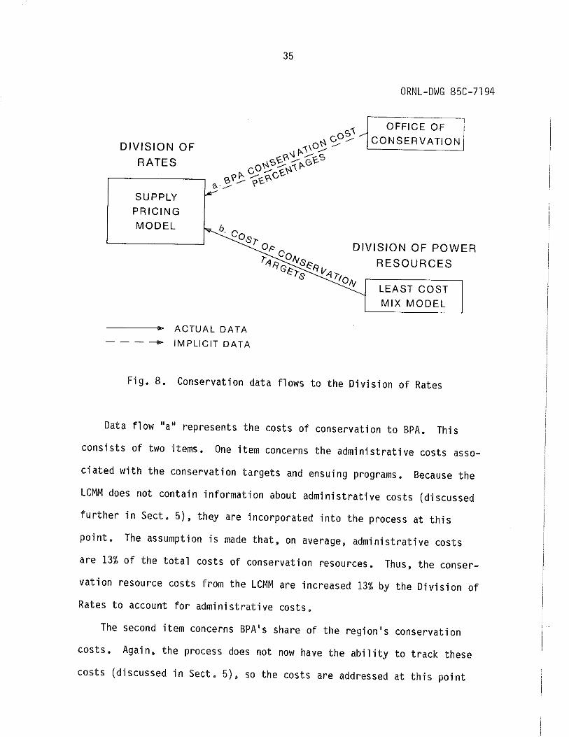
3,5 CONSERVATION DATA FLOWS TO THE DIVISION OF RATES
This subsection addresses conservation data which flow from the
Office of Conservation and the Divison of Power Resources to the
Division of Rates and its Supply Pricing Model (Fig. 8).
*such a model might be the Hourly Electric Load Model (HELM) that is used by the Division of Power Forecasting.
DIVISION OF RATES
SUPPLY PRICING MODEL
ACTUAL DATA
---- IMPLICIT DATA
35
ORNL-DWG 85C-7194
,--~~~~-~l
OFFICE OF ' CONSERVATION
DIVISION OF POWER RESOURCES
LEAST COST MIX MODEL
Fig. 8. Conservation data flows to the Division of Rates
Data flow "a" represents the costs of conservation to BPA. This
consists of two items. One item concerns the administrative costs asso-
ciated with the conservation targets and ensuing programs. Because the
LCMM does not contain information about administrative costs (discussed further in Sect. 5), they are incorporated into the process at this
point. The assumption is made that, on average, administrative costs
are 13% of the total costs of conservation resources. Thus, the conser-
vation resource costs from the LCMM are increased 13% by the Division of
Rates to account for administrative costs.
The second item concerns BPA's share of the region's conservation
costs. Again, the process does not now have the ability to track these
costs {discussed in Sect. 5), so the costs are addressed at this point
36
in the process. Currently, it is assumed for modeling purposes that
100% of the conservation costs from the LCMM associated with signer uti
lities* are BPA costs.
Data f1 ow "b" contains the cost data output from the LCMM re 1 a ted to
acquiring F3 conservation resources. These numbers are altered by the
Division of Power Resources to better fit the SPM's financing format.
Using data from the LCMM output and the Power Resources supply curves,
$/year (1980-$) required for conservation acquisition for each sector
are calculated. These figures are increased to account for inflation
(6%/year). It is assumed that BPA will borrow money each year to meet
these expenses. Therefore, annual payments over a 20-year period given
yearly specific borrowing rates (supplied by Data Resources, Inc.) are
calculated for each conservation expense for each sector. The payments
are aggregated by sector and split by signer and nonsigner utility
before they are sent to the Division of Rates. The signer and nonsigner
costs are split based on the weighted average of the last three years of
historical load.
3.6 EVALUATION OF THE MODELING PROCESS
The material presented in Sections 2 and 3 indicates that the BPA
modeling process is large and complex. The process encompasses many
types of sophisticated mathematical models and large quantities of data
flow through and are transformed by the models. Our work to document
the use of conservation data in the process leads us to three conclusions.
*utilities in the BPA service area choose whether to participate in BPA conservation programs. A signer utility has chosen to participate, a non-signer utility has chosen not to participate.
37
First, given the level of detail in CON-179, we found no inappro
priate or inconsistent uses of conservation data. There are no explicit
instances of double counting for price induced conservation or trans
mission line losses, for instance, and the process properly respects the
units of measurement for all the data encompassed within it. The
remarkable integrity of the system is attributable to the competency of
and communication among BPA's technical staff. During our interviews
between September 1984 and March 1985, we observed a high degree of
staff interaction within and between offices and divisions. Interaction
typically focused on the data "handoffs" between models with the goals
of identifying the units of measurement or data to be transferred, spe
cifying the formats of the transfers, and determining the timing of the
transfers. This interaction resulted in a process high in integrity;
the process performs as BPA staff perceive it should.
Our second conclusion qualifies the first. It is possible,
although we believe improbable, that the process encompasses inappro
priate and/or inconsistent uses of conservation data that we did not
discover because we did not delve into the process deeply enough to rule
out all possible problems. For example, the actual construction, number
by number, of the 38 supply curves and the associated market penetration
ramps is not presented here. The algorithms used by the residential
demand model to choose fuels, by the Division of Power Resources to
transform LCMM conservation costs for input into the Supply Price Model,
and by the Program Mix Model to construct conservation programs were
also not presented here.
Our third conclusion is that the process could stand improvement.
This is not surprising to anyone who has worked in modeling energy
38
processes. First, the process encompasses many judgments that are not
supported empirically (e.g., those relating to price induced conser
vation) but were necessary to maintain the integrity of the process.
Second, as discussed in the next five sections, other judgments were
made to reduce the complexity of the process, at a cost of not accur
ately describing the real world aspects of the process. Third, not
addressed in this report are problems of using information produced by
the process for purposes of policy analysis and debate.

39
4. OFFICE OF CONSERVATION AND DIVISION OF POWER FORECASTING PROCESS ISSUES
4.1 INTRODUCTION
Sections 2 and 3 highlight the extensive interactions that occur
among various divisions of the BPA in the conservation/load/resource
planning process. Analysis of the interactions between the Office of
Conservation and the Division of Power Forecasting and within the Office
of Conservation reveals three areas of potential improvement. The first
concerns interactions between program planning in the Office of
Conservation and demand forecasting in the Division of Power
Forecasting with respect to modeling price induced conservation, fuel
switching, and take back behaviors. The second area pertains to main
taining consistency between Conservation's supply curves and Power
Forecasting's technical potential curves. The third area of discussion
focuses on how the Office of Conservation could accommodate potential
changes over time in program participant characteristics.
4.2 PRICE INDUCED CONSERVATION, FUEL SWITCHING, AND TAKE BACK BEHAVIOR PROCESS ISSUES
Conservation program planning and Power Forecasting have numerous
mutual areas of concern, including the modeling of price induced conser-
vation, fuel switching, and take back behaviors. Conservation and Power
Forecasting tackle these modeling areas interdependently, as described
in Sect. 3.3. However, the modeling process handles these three topics
in a deficient manner. A solution to the problems reviewed below is to
adapt the demand models to incorporate explicitly the existence or
potential existence of conservation programs.
40
The concept of price induced conservation behavior arises from BPA's
desire not to pay for conservation that would have occurred without BPA
conservation programs. Price induced conservation refers to energy con
sumers' energy conservation investments which are prompted solely by
market forces (e.g., energy price changes, technical improvements).* As
described in Sect. 3, this behavior is an important concern for both the
Office of Conservation and the Division of Power Forecasting. To recon-
cile price induced behavior forecasts made by the energy demand models
and with the potential existence of conservation programs, the two organi-
zations decide together how much to reduce the maximum market penetra-
tion conservation potentials which are used to create the supply curves.
This approach may be deficient in three ways. First it is possible
for energy demand models (the residential and commercial models in par
ticular) to forecast consumer energy investment decisions that result in
more or less price induced conservation than was agreed upon. This
problem exists because the demand models do not explicitly predict spe-
cific measure installation; they only model changes in relative energy
efficiency (e.g,, per house) due to price changes. Thus, reducing
market penetration potentials to reflect forecast price induced behavior
entails a significant degree of judgment.
Second, the existence or probable existence of conservation programs
over time may significantly alter price induced conservation through
feedback effects. For example, program participation could so substan-
*Price induced conservation also refers to the market simultaneously providing more energy efficient products (e.g., appliances) and discounting less energy efficient products. Trends in market production are essentially driven by national prices.

41
tially reduce energy consumption for participants (or the anticipation
of program participation could suggest such substantial energy consump
tion reductions) that demand model forecasted price induced conservation
may never be realized. This problem exists because the demand models do
not explicitly treat the existence (actual or potential) of conser
vation programs.
Third, actual conservation programs may intentionally include some
measures that could be considered price induced (e.g., shower flow
restrictors or water heater jackets). The current process could double
count the effects of these measures because the demand models cannot be
adjusted accordingly.
Thus, two potential problems exist in modeling price induced conser
vation. First, there can be overlaps or gaps between the energy demand
models' forecasts of consumer energy investments, what Conservation
assumes to be price induced behavior, and what in reality is the beha
vior. Results of BPA conservation program evaluations could help iden
tify any gaps or overlaps. For example, analysis of home energy audit
data could indicate commonly installed energy conservation measures
before a BPA subsidized retrofit. Data collection and analysis of
retrofit behavior of non-participating households and perceptions of
future BPA program offerings held by potential program participants
could also be useful.
Second, the energy demand models do not include the existence and
possible existence of conservation programs over time. Both problems
could result in inaccurate demand forecasts and inaccurate predictions
about the performance and penetration of conservation programs. A
42
potential solution would be to explicitly incorporate conservation
programs in the demand models and let the models forecast price induced
conservation in this environment. One way to accomplish this task might
be to develop a discrete choice methodology that models consumer program
participation choices. Such choices would have to be related to other
behavior, such as fuel choice and equipment utilization.
Modeling fuel switching and take back behavior suffers from similar
problems. Fuel switching refers to consumers changing fuel types for
significant energy consuming activities (e.g., space heating and water
heating). Take back behavior refers to possible smaller than expected
decreases in energy consumption by households and/or businesses after
participation in a BPA conservation program or after installation of
non-subsidized energy conservation measures.
A problem with accounting for fuel switching and take back in the
current process is that the behaviors are demand modeled over time
without inputs that describe existing or potential conservation
programs. At present, only energy prices, utilization elasticities, and
technical efficiencies affect fuel switching and take back in the demand
models. However, program participation can also influence this behavior.
For example, a household participating in a BPA residential weatheriza
tion program in 1990 may obtain a large enough decrease in electricity
costs that it will not switch from electricity to wood or natural gas
even if faced with rising electricity prices or increased usage of
electricity due to new end use demands.
Solutions to the problems are nontrivial. With respect to all three
issues, two actions appear desirable. Either the energy demand models
43
could be modified to incorporate the measures that each conservation
program might subsidize, or the energy demand models' decision algorithms
could be modified to represent the characteristics of existing and
potential conservation programs. In addition, better coordination and
communication between Conservation and Power Forecasting concerning
these common modeling issues could reduce possible modeling errors.
4.3 REPRESENTING THE TECHNICAL POTENTIAL OF CONSERVATION IN CONSERVATION PROGRAM PLANNING AND POWER FORECASTING
Conservation supply curves (Office of Conservation) and technical
efficiency curves (Division of Power Forecasting) are similar in that
both relate technical improvements in building shells and energy using
equipment to cost and both model the nature and extent of cost efficient
energy conservation investments. However, there is concern that the
technical efficiency curves and supply curves may be inconsistent in
ways that affect the integrity of the modeling process. For example,
the residential technical efficiency curves were developed using the
Northwest Power Planning Council's residential heat loss methodology and
Conservation's residential supply curves were developed using BPA's
standard heat loss methodology. Thus, a concern is that the different
heat loss methodologies may yield inconsistent estimates of conservation
potential between the demand model and the supply curves. A more in
depth analysis is needed to explore this possible inconsistency. There
is not a data base problem in the commercial sector because curves were
developed for both power forecasting and conservation program planning
using the same data and methodology.
Regardless of how supply and technical efficiency curves are developed,
an important point is that in practice the technical efficiency curves

44
and the supply curves should not necessarily be identical. Basically,
this is because the technical efficiency curves encompass all fuel types
and associated technologies and all of the region's energy consumers
because the demand models encompass all the region's energy consumers.
The supply curves, on the other hand, only incorporate energy conser
vation measures that BPA can offer through programs to reduce electri
city consumption and in the future may only include consumers eligible
for BPA conservation programs. Thus, supply curves can be viewed as a
subset of the technical efficiency curves and may not be expected to
resemble closely the technical efficiency curves.
Differences between the two types of curves may also be rationalized
because they perform different roles in the mode 1 i ng process. The tech
nical efficiency curves nominally represent technology available to
energy consumers and the demand mode 1 s predict how consumers will use
the information to make equipment efficiency and thermal shell effi
ciency decisions. Thus, the technical efficiency curves form a set of
technologies characterized by cost and efficiency to do a certain task
(e.g., provide ceiling insulation). The supply curves, on the other
hand, specify one technology per task at one cost because conservation
programs cannot be run with complicated technological and cost options
for each class of energy conservation measure.
A potential problem that may require rectification exists between
the two sets of curves. The technical efficiency curves in the residen
tial and commercial energy demand models are developed with respect to
proven technological potentials. In other words, these curves encompass
efficiency improvements that may not yet have been introduced in the

45
market but which have been demonstrated experimentally. The supply
curves, though, are developed with technologies currently available in
the marketplace. This is reasonable because the measures constituting
the supply curves would have to be installed via a conservation program
if the curve is selected by the Least Cost Mix Model. Given the respec-
tive goals of Power Forecasting and Conservation, these differences may
not be reconcilable.
4.4 CONSERVATION PROGRAM PLANNING PROCESS ISSUES WITHIN THE OFFICE OF CONSERVATION
The processes within the Office of Conservation might be improved
regarding the relationship between supply curves and conservation
program activities over time. Of particular importance is the change in
program participants over time. Since the supply curves are developed
independently of any knowledge of future conservation programs, the con
servation potentials over the 20-year planning horizon are represented
by a fixed average potential per participant (or ft2 in the commercial
sector, for example) over time. Thus, a participant in 1988 is impli
citly assumed to have the same conservation potential as a participant
in 1995. In reality, however, this will not be the case. For instance,
those with greater conservation needs may participate sooner in the
program. If this is so, an average figure will not correctly represent
conservation over time.
A solution to this problem should address the issue of self-
selection. For example, average weather-adjusted savings for 1982 BPA
Residential Weatherization Program participants is close to 4900
kWh/year, while the figure for 1983 participants is around 2700 kWh/year

46
(Tonn, Hirst and Holub 1985}. It is possible that 1982 participants
need to save energy more than the 1983 participants. If self-selection
is expected to continue, then supply curves would need to be adjusted
over time.

47
5. CONSERVATION DATA FLOW ISSUES
5.1 INTRODUCTION
There are several areas where additional detail might improve the
conservation planning process. One is incorporating more detail about
four types of conservation costs. Another is more accurately repre
senting energy conservation measures in the Least Cost Mix model. None
of the topics mentioned in this section would require BPA to alter the
current process in any significant way nor would any of the issues
require BPA to change substantially any conservation policies. However,
the changes would require the commitment to collect more data and expand
the process to include the added detail.
5.2 CONSERVATION COST DATA FLOW ISSUES
Four energy conservation costs could be represented with more detail
in the conservation planning process to improve the modeling process.
The four costs are conservation program administrative costs, the con
servation cost advantage, line loss costs, and BPA vs regional conser
vation costs.
The first three costs are interdependently represented in the pro
cess. Conservation program administrative costs are assumed to average
13% of total program costs. The conservation cost advantage arises from
the Pacific Northwest Power Planning and Conservation Act of 1980 which
gives conservation a 10% cost advantage over other power resources in
the Pacific Northwest. Thus, a dollar's worth of conservation cost is
represented as 90 cents when BPA chooses the least cost mix of power
resources to meet the region's power demands. Reduction of electricity
transmission line losses by 6.7% due to conservation translates into a
48
6.7% reduction in the costs of conservation. These three conservation
costs are interdependent because the current process assumes the three
costs cancel each other out; the administrative costs may be seen as
increasing conservation costs relative to other resources while the
other two costs decrease the relative cost of conservation. Therefore,
no costs are represented explicitly in the data that the Office of
Conservation sends to the Least Cost Mix model.
The major deficiency with this arrangement is that administrative
costs could be specified more accurately. Some BPA conservation
programs may have relatively high administrative costs (e.g., programs
that only supply a few measures). Other programs may have relatively
small administrative costs, especially those that purchase large amounts
of energy conservation measures. Thus, programs may not always average
13% administrative costs, and it is also not likely that the supply
curves that incorporate the measures associated with the programs
average 13% administrative costs. By not including administrative costs
within the supply curve costs, the LCMM is provided misleading infor
mation. Measures associated with programs with high administrative
costs have an advantage over measures associated with programs with less
administrative burden. Determining average administrative costs per
supply curve would yield a process that describes better actual conser
vation costs and would, therefore, permit a more efficient selection of
resources.
Explicitly representing administrative costs in the Least Cost Mix
Model would require that the conservation cost advantage and the line
loss costs also be treated explicitly. The former could be directly
49
incorporated into the LCMM objective function by reducing the cost
parameters by 10%. (Conservation costs transferred from the LCMM to the
SPM would then need to be increased 10%.) The line loss factor could
also be handled this way if it is too difficult to associate line losses
with different supply curves.
Currently, all the conservation costs in the LCMM are regional, not
just BPA, costs. Not currently distinguishable are costs of conser
vation assumed to be borne by program participants, by utilities, and by
BPA. Also, costs are not distinguished between signer and nonsigner
utilities. (It is possible that costs for conservation measures and their
installation vary between signer and nonsigner utilities.) Because
costs are not discernable, the current process does not allow the LCMM
to determine the optimal BPA financial allocation of resources to con
servation.
It would be more logical to represent separately signer and non
signer conservation costs during the conservation planning process.
This is not a straightforward goal, however. One problem would be to
develop supply curves which only include conservation potential
available from signer utilities. Currently available data sets are pro
bably not sifficient to allow rigorous decomposition across all energy
consuming sectors. Costs associated with nonsigner utilities could be
included as a constant in the LCMM or eliminated altogether from the
analysis.
Adapting the process to separate BPA costs from utility costs and
consumer costs within the programs would also be difficult even though
such data is available from program evaluations. This is because the

50
measures that compose the supply curves are not correlated exactly with
conservation programs. Thus, work would be needed to find out exactly
how much of the costs associated with a supply curve are actually utility
and consumer costs.
5.3 ENERGY CONSERVATION MEASURE DATA FLOW ISSUES
This subsection addresses three data flow issues associated with
representing energy conservation measures in the conservation planning
process. The issues are: changing ECM performance over time, costs of
ECMs over time, and development of subregional supply curves. Action on
each of these issues could result in a process that more accurately cap
tures energy conservation measure effects and potentials.
The ability of an ECM to save energy may change over time. For
example, weatherstripping may become less effective as portions become
brittle and/or torn away from surfaces. Depreciation may not occur all
at one time, as the concept of ECM lifetime might suggest. Instead,
performance may di mini sh gradually, a fact not currently incorporated in
the planning process. Measure performance may also increase over time
as users learn to use the measure. An example may be irrigation sche
duling. Not accounting for measure performance depreciation of appre
ciation could result in inaccurate conservation forecasts in the
mid-to-long term.
Depreciation and appreciation rates could be incorporated into the
supply curves; data would need to be collected to support this task.
Since the measures included in a supply curve differ with respect to
depreciation and appreciation rates and lifetimes, a necessary step is
determining how to aggregate and average rates for each supply curve.
51
Closely re 1 a ted to changes in ECM performance is the issue of ECM
costs (installation and replacement) over time. Currently, it is
assumed that the real costs of ECMs will not vary over time; that
* is, ECM costs will change exactly as the genera 1 price index changes.
It may be important, though, to estimate accurately the real changes in
ECM costs. For example, if real costs are declining, it may be prudent
for BPA to invest in conservation at some later date. However, if real
costs are increasing, purchasing conservation in the near term may be
wise. Changing costs associated with supply curves can be adjusted
easily before the curves are sent to the LCMM. The problem is esti
mating the changes. It might be worthwhile for BPA to collect data
about price histories of a small set of ECMs and similar products and
predict potential cost changes.
The third issue pertains to subregionalizing the supply curves.
Currently, the curves represent the entire region. Prob 1 ems might arise
from this aggregation because different subregions can have different
conservation potentials. For example, housing construction and climate
variations across subregions can result in different conservation poten-
tials and costs. In addition, subregions may differ in the amount of
conservation that has already taken place. The point is that more spe-
cialized information about subregional conservation potentials can
*Economic theory, on the other hand, suggests that subsidized markets provide incentives for real cost increases relative to nonsubsidized markets. Thus, some energy conservation measures subsidized by BPA may increase in cost in real terms relative to other products sold in the Pacific Northwest.
52
result in greater actual conservation savings.* Using more supply
curves in the process would not be difficult. Instead of 38 curves, the
LCMM would have to consider 76 curves, for example. The major task
would be to collect data to support the subregional curve construction.
The 1983 Pacific Northwest Residential Energy Survey (1984d) may be
comprehensive enough to permit subregionalization in the residential
sector. More comprehensive data bases in other sectors may be required,
though. Before embarking on this task, however, BPA must be convinced
that the added burden upon the modeling process will be more than com-
pensated by improvements in conservation potential estimates. BPA must
also decide whether it can politically support "overconserving" in one
subregion and "underconserving'' in another.
*supply curves may also be broken down by investor-owned utilities, publically owned-generating utilities, and publically ownednongenerating utilities. This breakdown is roughly by climate (e.g., public-nongenerators are mostly east of the Cascades) and would allow better planning with respect to signer-nonsigner utilities (e.g., currently, no investor owned utilities participate in the BPA residential weatherization program).

53
6. ISSUES ASSOCIATED WITH MODELING CONSERVATION BEHAVIOR
6.1 INTRODUCTION
Demand side planning is concerned with how consumers make decisions.
Consumers make decisions about how much energy to consume, or, more
accurately, about when and how much to use energy consuming equipment.
Consumers also make decisions about program participation, retrofitting,
and behavioral changes. Therefore, it seems reasonable to consider
demand side planning from the viewpoint of understanding and influencing
consumer decisions.
BPA conservation program planning could be improved by more
rigorously using consumer decision making models. If use of such models
increases, care must be taken to develop models consistent with good
modeling practice and with models used by other offices within BPA,
especially those used by the Division of Power Forecasting.
6.2 OPPORTUNITIES FOR INCORPORATING CONSUMER DECISION MAKING FACTORS INTO CONSERVATION PROGRAM PLANNING
This subsection addresses the benefits of incorporating decision
making factors into conservation program planning models. As one
example, benefits to modeling program penetration rates via decision
models are discussed. Also discussed are conservation program marketing
spillover effects and consumer expectations about future energy prices
and conservation programs.
An important element in conservation program planning is predicting
consumer response to each program. Will the response be very light in
the beginning stages of the program or will the program be an instant
success? To help answer these questions, the Office of Conservation

54
developed a model that describes program penetration over time. Given a
program starting date, a ramp defines the percentage of the eligible
population that participates in a program over time (see Fig. 5}. Any
particular ramp resembles an S-curve because this shape incorporates the
idea that the growth of a program starts slowly, picks up over time, and
ends slow. The ramping model was estimated using conservation program
experience from U.S. utilities other than BPA (AMS, 1983}.
The ramping model was not developed using a model or theory of con
sumer decision making in any explicit manner. The model does not posit
what the goals or motivations of the particular consuming sector might
be nor specify what aspects of a conservation program might affect con
sumer decisions. For example, what type of incentive is used (if any)
and what is the incentive level? What are consumers' attitudes about
the convenience of obtaining program services and the reliability of
saving energy via retrofit? Because the model does not contain
variables such as these it cannot show how changes of such variables
affect consumer decisions.
One conclusion is that the ramping model may not describe very well
future program participation in BPA programs. After all, BPA programs
are unique as are the circumstances faced by the consumers in the
Pacific Northwest. Another important conclusion is that program planning
takes place without sufficient appreciation of consumers' decision
making behavior. Different program aspects could be determined after
studying goals and motivations of consumers eligible for various programs.
When viewing aspects of program planning from a consumer decision
making perspective, other important consumer decisions become more
55
amenable to analysis. One issue concerns how consumers integrate expec
tations about future energy prices and future BPA conservation program
offerings into their energy consumption decisions. For example, expec
tations of an energy price increase might induce consumers to reduce
energy consumption through a combination of behavioral changes and tech
nology improvements. However, if it is likely that BPA will offer
substantial subsidies for technological improvements, consumers may
eschew price induced conservation and wait for the BPA program.
Understanding how such factors influence decisions would help BPA pre
dict program participation responses and design the most cost efficient
programs.
Another issue concerns program participation decisions made in an
environment containing numerous conservation program offerings. BPA
runs over 20 different conservation programs, each marketed to a sector
of the consumer population. Decision makers in one target population
may also be in another target population. For example, one individual
may be a home owner, a farmer and own a small commercial enterprise.
The combined effects of conservation program marketing in the separate
sectors may have greater total effects upon this individual's decision
making than would be ascertainable from reviewing the individual
programs separately. "Information contagion" may also occur whereby a
program participant influences a nonparticipant into taking energy con
servation measures outside of a BPA program. In part, this saving is
attributable to the program. If issues such as these can be sorted out
and implemented in consumer decision making models, then BPA could
better plan its conservation programs and marketing strategies.

56
6.3 CONSISTENCY IN MODELING CONSUMER DECISION MAKING
In developing models of consumer decision making, several issues
might be addressed. One pertains to consistency about who makes the
decisions related to acquiring energy consuming technologies and energy
conservation measures. Another issue concerns consistency among models
developed by various parts of BPA which describe decision making for the
same consumers. A third issue concerns developing models that are use
ful for prediction purposes and are valid descriptions of human behavoir.
Determining the decision maker is an important element in the
development of a consistent set of models. For example, to predict the
success of conservation programs associated with new housing, it may be
necessary to model capital investment and appliance purchase decisions.
Identifying who actually makes the decisions, the home builder or the
home buyer, or a combination of the two, is important because the
builder is likely to purchase less energy efficient technologies to
reduce construction costs than would the home buyer. Conservation
savings predictions and demand forecasts could be inaccurate and program
performance less effective if models fail to describe behavior of the
true decision maker.
Another area where this issue could be important is in the residen
tial and commercial sectors where there may be confusion about whether
programs are directed at owners, building managers, or occupants.
Absentee owners may not be interested in energy conserving capital
investments although renters would likely appreciate the energy savings.
In the industrial and irrigation sectors, decision maker questions could
arise about the producer of energy consuming technologies (e.g., irriga-

57
tion pumps) and the buyers. Thus, in most sectors, determining who is
the decision maker is important.
It is not enough to develop models that intelligently, but indepen
dently, represent the proper decision makers within BPA's extensive
modeling process. It is possible for different parts of BPA to model
the same decision in different ways, thereby leading to potential
problems with double counting, data collection, etc. For example, in
designing and predicting the effects of a conservation program, the
Office of Conservation could assume that homeowners use a particular
decision process to determine their participation and price induced con
servation activities. However, the residential energy demand model used
by the Division of Power Forecasting may adopt a different decision
process assumption to describe similar behavior. In addition to program
participation and price induced conservation behavior, fuel switching
and take back decisions could also be modeled differently. These
conflicts should be resolved to avoid situations where different behav
iors for the same consumers facing the same decisions are predicted.
The development of models to describe consumer decision making is
still very much an art. Although probably beyond the main theme of this
report, a few words on the practice of decision model development would
be useful at this point. An issue that has gathered much recent atten
tion is the validity of human decision making models describing actual
decision making. For example, the Oak Ridge National Laboratory resi
dential energy model (Section 2} has a module that predicts residential
technical efficiency choices. The module assumes that homeowners choose
an efficiency level that minimizes life cycle costs. This assumption
may be convenient for modeling purposes and, indeed, may be the most

58
practical assumption. However, one could argue that only a small por
tion of the population actually uses this heuristic, given that it assumes
that decision makers assess many years of future energy prices for
several fuels, are able to specify their personal discount rates, and
can specify future operation, maintenance, and replacement costs.
A similar argument surrounds the use of other widely used modeling
schemes. The most prominent debate concerns the use of utility theory
to describe consumer decision making. Economists argue that utility
theory provides a valuable mathematical foundation from which to derive
statistically robust models of consumer demand. Opponents argue that
utility theory posits human information processing abilities well beyond
actual abilities (e.g., Simon, 1979, 1976; Steinbruner, 1974} and that
other models may be more descriptive of actual decision making behavior
(Stern and Aronson, 1984; Tonn, 1984; Tonn and Berry, 1984}.
An advantage of a decision model that corresponds closely to actual
decision making behavior is that it allows more accurate descriptions of
not only what happens, but also why and how it happens. This added
insight can be invaluable during program planning, evaluation, and
adjustment. The conclusion is that it is important to both understand
that decision making models could significantly benefit conservation
program planning and that developing models is an art requiring careful
consideration.
6.4 DISCUSSION
Developing consumer decision making models to support conservation
program planning is a challenging activity. Two ways for BPA to begin
to learn about the decision making characteristics of Pacific Northwest
59
customers could be to do survey work and analyze appropriate program
evaluation data. For example, surveys could be developed to collect
data on what consumers consider good and bad aspects of conservation
programs and on decisions made under a variety of hypothetical program
offerings. Survey data and evaluation data that BPA has on hand could
provide a foundation for this work.
Evaluations offer a wealth of data. For example, retrofit data
collected from households in Connecticut provided the basis for a model
describing the way households make retrofit decisions (Tonn and Berry,
1984). Similar studies could be done with BPA program evaluation data.
Such studies could explore zero interest loan acquisition by households
in BPA's Pilot Residential Weatherization Program, request for audits by
households in the Hood River Conservation Program, and retrofit measure
selection strategies used by households in the Interim Residential
Weatherization Program.


61
7. CONSERVATION RESOURCE PLANNING ISSUES
7.1 INTRODUCTION
Two issues might suggest major changes in BPA conservation resource
planning. The first concerns using supply curves to represent conser
vation in the Least Cost Mix Model. The second issue concerns inclusion
of conservation program uncertainty in the LCMM. BPA action on either
issue would require substantial staff time to define the issues more
precisely and include the issues in the modeling process.
7.2 USING SUPPLY CURVES IN THE LEAST COST MIX MODEL
7.2.1 Introduction
The issue under consideration is whether or not representing conser
vation in the LCMM is better accomplished using supply curves or a
methodology that represents actual and/or potential conservation
programs. This subsection begins with a discussion of seven problems of
using supply curves to represent conservation resources. A conservation
program methodology could overcome these problems but at the cost of
possibly introducing new problems into the conservation resource
planning process.
7.2.2 Seven Problems with Supply Curves
Representing conservation in the LCMM using supply curves results in
at least seven problems. The first problem arises from the nature of
the supply curves. These curves are developed by analyzing the cost to
conserve energy through installation of various energy conservation
measures (ECMs). When the LCMM allocates resources to acquire the
62
conservation associated with a particular supply curve, it is actually
choosing a set of measures around which a conservation program should be
developed. The problem is designing conservation programs which closely
correspond with the measures associated with the selected supply curves.
For example, the set of curves selected may call for a mix of measures
including T wall insulation, U storm window, and V weather stripping
installations to conserve X kWh in a given year. Even though this goal
is technically feasible, the job of mapping the supply curve measures
into programs may be quite difficult.
Second, it is possible for the LCMM to choose a set of supply curves
and conservation targets that cannot be met with any set of conservation
programs because of administrative and program participation constraints.
If this situation arises, the Office of Conservation must place additional
constraints upon the supply curves given to the LCMM and request that the
LCMM be rerun. This would be time consuming for all participants in the
modeling process.
The third problem concerns using supply curves to represent uncer
tainty of conservation in the LCMM. One source of uncertainty associated
with conservation program planning is the technical performance of the
ECMs (i.e., will measures save as much energy as expected?). A probabil
ity distribution of performance for each supply curve could be repre
sented in the LCMM constraints and objective function (Sect. 7.3).
However, most sources of conservation uncertainty are not related to
technical expectations, but rather to aspects of conservation programs.
For instance, how many measures will be installed each year and how will
consumer energy-using habits change after ECM installation? Have the

63
contractor and utility costs been accurately estimated and have the
markets for the ECMs been accurately estimated? Uncertainties asso
ciated with these questions are difficult to model in the LCMM using
supply curves because they are not measure oriented. Rather, they per
tain to administrative matters, marketing strategies, and population
responses.
The fourth problem concerns the consistency between the concepts of
supply curves and supply curve ramps. In the current LCMM, the contribu
tion of a supply curve changes over time as the curve is ramped in via
market penetration ramps. Thus, given a certain resource allocation,
cumulative energy savings associated wtih a curve may increase slowly in
the near term, quickly in the mid term, and slowly in the long term.
The ramping idea is supposed to capture the fact that there are early
adopters, middle-of-the-roaders and laggards with respect to conser
vation technology adoption.
Unfortunately, the market penetration ramps that are so intimately
related to the concept of a conservation supply curve are not well
related to actual program performance. Essentially, the ramp idea is a
poor substitute for what is really happening: that BPA and utility
administrators are setting up program operations and consumers are
making decisions about participation. Ramps, and therefore the supply
curves, do not encompass explicitly these behaviors because they are not
developed with respect to actual programs and consumer decision making.
The fifth problem is the difficulty in associating administrative
costs with supply curves. As discussed in Sect. 5, some programs may

64
have more or less administrative costs per kWh saved than other programs.
However, it is hard to associate administrative costs with a supply
curve because each curve is estimated without reference to actual or
potential programs and more than one program may be needed to cover all
the measures in a curve.
The sixth problem arises from the difficulty in deriving the effects
of supply curves upon loads. Measures encompassed in a supply curve may
have differing effects upon peak and seasonal loads. These effects
could be aggregated for a curve, but if the programs designed to meet
supply curve targets do not exactly match a supply curve's mix of
measures, then the actual load effect will be different from the effect
suggested by the supply curve.
The seventh and last problem mentioned is that supply curves cannot
easily incorporate potential new electricity demands because explicit
measures must be envisioned to conserve energy with respect to specific
end uses. An idea of a technology possibly existent 15 years from now
may not allow for the required specificity. This problem may not
impact supply curves as much as the demand forecasts, however, because
in conservation an unrepresented technology is just an ignored poten
tial. No extraordinary problems in conservation prediction would result.
On the other hand, ignoring new demands in power forecasting could
result in significant underestimates of demand.
7.2.3 Discussion
These seven problems do not render the use of supply curves in the
LCMM valueless, and the supply curve practice may well be the most cost
efficient method. However, it is worth reviewing the possibility of
65
representing conservation in the LCMM using constraints that relate
directly to conservation programs. For example, one set of LCMM
constraints could relate to the Residential Weatherization Program. For
every dollar spent in the program, electricity savings could be esti
mated and a constraint could be specified to maintain a minimum viable
program. Appendix A presents a formulation to represent conservation
programs in the LCMM.
Representing programs in the LCMM would directly eliminate the first
two problems mentioned above, inconsistency of supply curves with
programs and the possibility of choosing conservation resources una
vailable from conservation programs. The fourth and fifth problems
would also be eliminated because ramps would be replaced with program
performance estimates and administrative costs could be directly asso
ciated with programs. The third problem, representing uncertainty,
could also be ameliorated because each aspect of program uncertainty
could be represented explicitly in the program's LCMM constraints
(Sect. 7.3). It would be easier to determine load effects, too,
because they would be estimated for each program. With respect to
problem seven, incorporating new uses, it is not clear whether or not
representing programs would be a significant benefit.
Implementing program constraints raises many significant problems,
not the least of which is determining what is meant by a program. The
number of constraints required to represent programs in the LCMM could
become large and complex, if many types of incentives and levels of
incentives as well as program eligibility requirements are to be con
sidered for each program. Instead of the 38 supply curves now used,

66
variations on a small number of basic programs could result in 100 or
more program curves, by analogy.
Another problem with implementing program constraints is having to
design programs which may never be implemented. To provide the LCMM
with a comprehensive set of programs, programs would have to be designed
with the idea that many may never be chosen by the LCMM, Of course, it
is possible to accomplish such an exercise, but it may not be cost
effective. In summary, using program constraints could eliminate signifi
cant problems associated with using the supply curves in the LCMM.
However, proyram curves would entail much new work by the program
planning staff.
7.3 UNCERTAINTY IN CONSERVATION PROGRAM PLANNING
7.3.1 Introduction
Dealing with uncertainty is an unavoidable aspect of conservation
program planning. We present two complementary methods of dealing with
uncertainty related to the cost and effectiveness of ECMs. One method
represents uncertainty in the LCMM constraints associated with conser
vation. The second method represents the costs of conservation program
uncertainty in the LCMM objective function.
An important assumption is that conservation uncertainty should be
represented explicitly in the modeling process. The present process
does incorporate uncertainty, but only implicitly. In determining
conservation estimates of cost and performance, conservative conser
vation estimates are typically made. In other words, the estimates
represent highly likely program outcomes (e.g., costs should not exceed

67
$X and savings should not be less than Y MW) but not the best guess out
comes, One can argue that building into the process conservative esti
mates is adequate. On the other hand, with more complete information
about uncertainty, policy makers could plan better. Thus, in the long
run, it may be cost efficient for BPA to represent uncertainty expli
citly in the process.
7.3.2 Representing Uncertainty in Least Cost Mix Model Constraints
The motivation for representing conservation uncertainty in the
LCMM's constraints is to prevent the LCMM from choosing a set of supply
curves (or programs) with a combined risk which is unacceptable to the
conservation program planners. For example, the LCMM could choose a set
of supply curves that offer a 10% chance of obtaining less than 75% of
the conservation needed to meet the load forecast. This allocation
could prove unsatisfactory if conservation program planners are able to
accept only a 5% chance of obtaining less than 75% of the expected con
servation. LCMM constraints could be developed to insure that the set
of chosen supply curves (or programs) would meet or exceed planners'
risk preferences.
The following five steps could guide development of such constraints.
The first step entails specifying probability distributions for the
expected energy savings associated with each supply curve. To do this,
the program planners would need to estimate two of the following three
numbers for supply curve energy saving - best guess, the expected guess
and the worst guess (Fig. 9). The best guess could relate to a five per
cent (or ten percent or whatever percentage is most comfortable) chance
of the supply curve savings exceeding a given energy savings level. The

X% PROBABILITY OF SAVINGS LESS THAN
'WORSE GUESS'
'WORST GUESS'
68
EXPECTED VALUE
OANL-OWG 85C-7512A
X% PROBABILITY OF SAVINGS GREATER THAN
'BEST GUESS'
'BEST GUESS' ESTIMATED ENERGY SAVINGS
(MW)
Fig. 9. Example of supply curve probability distribution.
expected guess would correspond to a 50% chance of exceeding or not
meeting another savings estimate. The worst could relate to a five
percent (or whatever is comfortable) chance of not achieving a low
energy savings estimate. These estimates and a distribution curve
assumption (assuming a normal curve, for example) permit probability
distributions for each supply curve to be constructed. The second step
entails calculation of the standard deviations for each distribution
given the estimated points and the assumed shape of the probability
distribution curve.
Step three entails determining minimum and maximum levels of accep-
table risk for conservation as a whole. That is, program planners
and/or other policy makers specify acceptable risks of not meeting
expected conservation savings or exceeding expected savings. For

69
example, the decision makers may view as an acceptable risk a 5% chance
of meeting less than 75% or more than 150% of total expected conser-
vat ion savings.
Step four is to insert two conservation constraints into the LCMM,
one for not meeting savings and one for exceeding savings. The left-hand
side of the former constraint would contain the sum of the 5% levels of
energy saving for all the conservation supply curves selected by the
LCMM (e.g., corresponding to the worst guess shown in Fig. 9). The
right-hand side would contain 75% of the sum of the expected values of
n n the chosen curves: k 5% guess for curve i > .75 L E(X)curve i.
i=1 - i=1
A similar process gives the exceeding savings constraint:
n k 95% guess for curve i < 1.5
i=1
n k E(X) curve i.
i=l
The fifth step entails optional sensitivity analysis, accomplished
by changing the risk preference parameters where a constraint is binding
or where a constraint renders the linear program infeasible.*
7.3.3 Representing Uncertainty in the Least Cost Mix Model Objective Function
The premise behind representing conservation program uncertainty in
the LCMM objective function is that there is a potential cost associated
*This process is only an introductory suggestion and includes at least one drawback that should be noted, To the degree that the supply curve uncertainty distributions are dependent, the constraints will not correspond exactly to the specified lower and upper risk levels for total estimated conservation savings. That is, the joint probability of obtaining lower (or upper) 5% (or 95%) levels on each supply curve distribution (as the constraint suggests) is less than 5% and decreases as the number of supply curves selected increases. This means that the method leads to more restrictive constraints than intended.

70
with uncertainty. As a rule, BPA desires to obtain the maximum amount
of conservation per dollar expended at the least possible risk. Thus,
given two conservation programs that provide identical expected amounts
of conservation at identical costs, BPA would prefer the supply curve
with the least risk. In a larger perspective, all power resources have
associated with them a degree of risk and BPA could experience a real
cost for acquiring a risky set of power resources. To account for the
cost of risk in the LCMM, BPA could include directly the cost of risk
associated with conservation or any resource within the objective func
tion. The question that this subsection explores is how to do this for
conservation. The following ten-step process is a useful guide (Table 1).
The first step entails running the LCMM with all the conservation
supply curves entered and the usual objective function. This step pro
duces a minimum system cost for meeting BPA load obligations with con
servation available.
Step two requires running the power forecasting models without any
conservation program inputs. The third step entails running the power
forecasting models with the conservation inputs selected in step one.
Step four entails subtracting the load forecast in step three from the
load forecast in step two to find the load value of conservation. As
shown below, this quantity represents the load reduction value of con
servation to the entire system and the monetary value of this reduction
will be used to calculate the cost of conservation uncertainty.
Step five develops a sampling distribution of total estimated supply
curve savings given the supply curves chosen in step one. The indivi
dual supply curve probability distributions could be constructed as
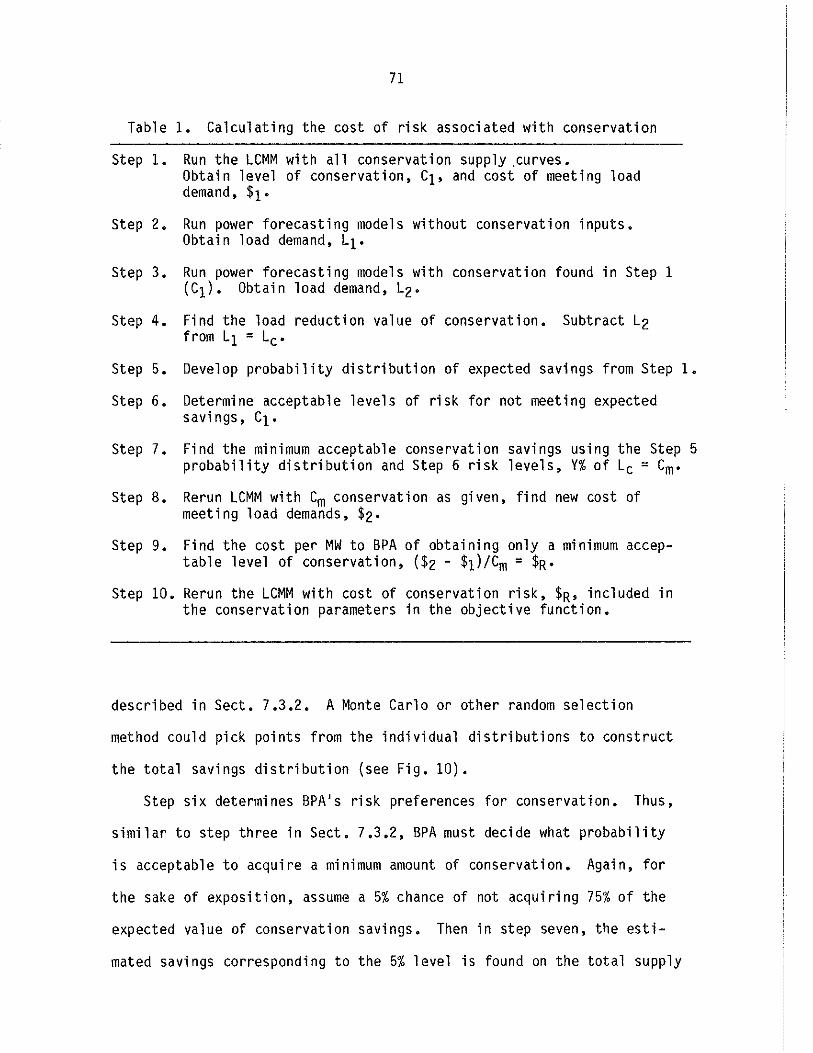
71
Table 1. Calculating the cost of risk associated with conservation
Step 1. Run the LCMM with all conservation supply ,curves.
Step 2.
Step 3.
Step 4.
Obtain level of conservation, C1, and cost of meeting load demand, h. Run power forecasting models without conservation inputs. Obtain load demand, L1.
Run power forecasting models with (Cl). Obtain load demand, L2·
conservation found in Step
Find the load reduction value of conservation. Subtract L2 from L1 = Lc·
1
Step 5. Develop probability di stri buti on of expected savings from Step
Step 6. Determine acceptable levels of risk for not meeting expected savings, C1.
Step 7. Find the minimum acceptable conservation savings using the Step probability distribution and Step 6 risk levels, Y% of Lc = Cm.
Step 8, Rerun LCMM with Cm conservation as given, find new cost of meeting load demands, $2.
Step 9. Find the cost per MW to BPA of obtaining only a minimum acceptable level of conservation, ($2 - $1)/Cm = $R•
Step 10. Rerun the LCMM with cost of conservation risk, $R, included in the conservation parameters in the objective function.
described in Sect. 7.3.2. A Monte Carlo or other random selection
method could pick points from the individual distributions to construct
the total savings distribution (see Fig. 10}.
Step six determines BPA's risk preferences for conservation. Thus,
similar to step three in Sect. 7.3.2, BPA must decide what probability
is acceptable to acquire a minimum amount of conservation. Again, for
the sake of exposition, assume a 5% chance of not acquiring 75% of the
expected value of conservation savings. Then in step seven, the esti-
mated savings corresponding to the 5% level is found on the total supply
1.
5
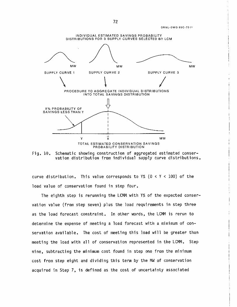
72 ORNL-OWG 85C-7511
INDIVIDUAL ESTIMATED SAVINGS PROBABILITY DISTRIBUTIONS FOR 3 SUPPLY CURVES SELECTED BY LCM
~ /\ ~'--MW MW
SUPPLY CURVE 1 SUPPLY CURVE 2 SUPPLY CURVE 3
\ \ I PROCEDURE TO AGGREGATE INDIVIDUAL DISTRIBUTIONS
INTO TOTAL SAVINGS DISTRIBUTION
X% PROBABILITY OF SAVINGS LESS THAN Y
y -X
TOTAL ESTIMATED CONSERVATION SAVINGS PROBABILITY DISTRIBUTION
MW
MW
Fig. 10. Schematic showing construction of aggregated estimated conservation distribution from individual supply curve distributions.
curve distribution. This value corresponds to Y% (O < Y < 100) of the
load value of conservation found in step four.
The eighth step is rerunning the LCMM with Y% of the expected conser
vation value (from step seven) plus the load requirements in step three
as the load forecast constraint. In other words, the LCMM is rerun to
determine the expense of meeting a load forecast with a minimum of con-
servation available. The cost of meeting this load will be greater than
meeting the load with all of conservation represented in the LCMM. Step
nine, subtracting the minimum cost found in step one from the minimum
cost from step eight and dividing this term by the MW of conservation
acquired in Step 7, is defined as the cost of uncertainty associated

73
with acquiring a MW of conservation.* The final step, is to run the
LCMM a third time, this time with the cost of conservation uncertainty
included in the conservation cost parameters in the objective function
to select new conservation supply curves.
This ten-step procedure could prove very time consuming for the BPA
staff. In addition, including the cost of conservation uncertainty will
put conservation at a disadvantage if the uncertainty costs for other
power resources are not also entered in the objective function.
Nevertheless, the benefits from representing uncertainty as a cost of
conservation could greatly improve policy making by explicitly ensuring
that BPA acquires power resources consonant with its acceptable levels
of risk.
*That is, if conservation produces a minimum of savings, the extra load must be supplied through other resources. The additional cost of employing those resources arises from the uncertainty of conservation performance.

75
8, MISCELLANEOUS CONSERVATION PLANNING ISSUES
8.1 INTRODUCTION
This section examines two general issues that do not fit into the
previous sections, The first concerns adapting the conservation
planning processes to allow analysis of nonconservation policy matters.
The second issue concerns conservation planning in a dynamic tech
nological environment.
8.2 CONSERVATION PLANNING WITH RESPECT TO NONCONSERVATION ISSUES
Planning conservation programs and representing conservation in the
larger BPA modeling process are extremely complex and challenging tasks.
Suggesting that conservation planners render the system even more
complex by introducing analysis of nonconservation issues is unwarranted
unless the potential for improvement is significant. Two issues appear
substantial enough for discussion: incorporating information about
BPA's cost of money into conservation program planning, and adapting the
modeling process to permit analysis of the impacts of various BPA poli
cies on power exports.
Ultimately, all of BPA's costs must be paid for by BPA customers in
the Pacific Northwest. In the short run, however, BPA can borrow money
from the u.s. Treasury, private financial institutions, and from the
utilities (by issuing billing credits) depending upon the nature of the
costs. The rate payers would benefit if, all else being equal, the
programs were funded by the least expensive source of money. The
effects on program design and operation of using different sources of
money could be explored via pilot programs, through surveys such as

76
those discussed in Sect. 6 concerning consumer decision making, and
through scenario studies.
The second issue involves possible substantial exports of BPA power.
If BPA pursues a policy of exporting power, it is also possible that
more conservation resources may be acquired via larger and more numerous
conservation programs. Conservation program planners could benefit by
having the ability to model on a contingency basis possible BPA export
policies.
A more detailed analysis of possible export policy indicates that a
policy could be quite complex. For example, the Natural Resources
Defense Council has suggested that only conservation obtained from
renewable energy sources should be available for export. Conservation
resource export constraints could be developed along other lines, too.
Perhaps only non-BPA financed conservation or only dispatchable conser
vation may be designated exportable. The conservation planning process
might be adapted to handle conservation-specific export scenarios. The
models then could be run under any of the export scenarios to predeter
mine how programs may be altered to match export targets.
8.3 CONSERVATION PLANNING IN A DYNAMIC ENVIRONMENT
From the viewpoint of the conservation planner, it would be prefer
able if the energy consuming environment were stable. That is, it
would be easier to develop conservation programs if technologies and
consumer behavior did not change over time. Unfortunately for the con
servation planner (but fortunately for the population as a whole}, the
technological and social environments are dynamic. This subsection
focuses on how changes in technology affect conservation program planning.

77
A real effect of technological change is the introduction of new
electricity uses. Examples in the residential sector include home com
puters, water bed heaters, and video cassette recorders. Such new uses
do not independently require the energy resources of space heating or
even water heating, but the sum of such uses might significantly
increase electricity demand.
Dealing with future energy demand is difficult enough without fore
casting new energy uses. Nevertheless, periodic analysis of tech
nological and consumer behavior trends could provide useful insights
into new demands. This investment could prove valuable if it uncovers
potential new uses that might rival space or water heating in energy
requirements. Any conservation measures that might be applied to new
technologies should then be incorporated into the supply curves. If
this exercise proves impossible, then new technologies should at least
be represented in the power forecasting models.
Associated with new and potential electricity uses are issues
related to possible dispatchable conservation technologies (i.e., con
servation which can be turned on and off to meet short term loads).
Most of BPA's load is supplied by dispatchable energy resources such as
hydro, coal, and nuclear which are brought on-line as needed. Conserva
tion resources, on the other hand, are nondispatchable and, therefore,
cannot contribute to the power system's flexibility in meeting system
loads. Future conservation technologies offer an opportunity to make a
portion of conservation dispatchable. For instance, the Tennessee
Valley Authority is conducting an experiment in Athens, Tennessee, in
which a small set of household ~ppliances are partially controlled by
the local utility. Although BP .. u~2s not now have a peak load problem,
78
developing the idea of dispatchable conservation resources could prove
valuable in the future.
The concept of not foregoing conservation opportunities flows con
veniently from the argument that BPA not overlook dispatchable resource
opportunities. "Foregone opportunities" refer to conservation oppor
tunities available today at a relatively high cost that will be una
vailable in the future at any cost. A good example of a policy
concerned with foregone opportunities is energy standards for new struc
tures. Energy savings obtainable at the time a structure is built, even
if costly at that time, may not be available or may be available only at
a very high cost at a later date when the savings would be needed.
Careful analysis is needed to identify potential foregone opportunities
and to determine the proper conservation program response.
The last issue is the need to create supply curves for completely
different sources of energy conservation. For example, a supply curve
might be developed to capture conservation potentials associated with
BPA's power transmission network.

79
9. ISSUE PRIORITIES
9.1 INTRODUCTION
This section focuses on the relative importance of addressing the
issues discussed in the previous five sections. Which issues might BPA
consider in the near term and which issues might be left for later con
sideration? Also, how difficult are the tasks associated with each
issue? Making these determinations is not straightforward. No data
exist to link resolution of an issue to quantitative improvements in the
BPA modeling system and the complexity of the modeling process makes
estimating task difficulty a difficult exercise. Because of these
problems, this discussion employs a simple categorical method to assign
a priority ranking to each of the issues.
The issues are divided into four groups, along two factors. The
first factor pertains to how difficult it might be to implement the
activities required to ameliorate an issue. Given the overall
complexity of the conservation process and its role in the larger BPA
modeling process, difficulty has been identified as "moderately dif
ficult" and "very difficult."
The second factor pertains to the expected benefits of accomplishing
the work associated with an issue. Because exact benefits are
unknowable, this factor has been structured along the concept of time;
the work on an issue could yield "immediate benefits'' or yield
"deferrable benefits." The term "immediate" indicates that work on an
issue could yield substantial benefits with a fairly high probability.
The term ''deferrable" indicates that potential work on an issue deserves
more discussion as to its merits or that the work could yield insubstan-

80
tial benefits. Figure 11 presents the issues considered in this section
by group.
9.2 MODERATELY DIFFICULT, IMMEDIATE BENEFIT ISSUES
There are several issues involving changes in the conservation
planning process that are minor compared with other issues and could
result in substantial improvements in the modeling process. Seven
issues are discussed in this subsection, two of which are characterizable
as process changes and five which pertain to new data.
The two process issues relate to representing better costs of con
servation e.g., BPA, utility, consumer (Sect. 5), and to improving con
servation program planning by updating the conservation supply curves to
respect changes in program participants over time (Sect. 4). The data
exist to support the activities associated with these two issues. For
example, a task associated with the first issue would be to add a data
link between the Office of Conservation and the Division of Rates and
its supply pricing model to specify costs by BPA program costs, non-BPA
costs associated with BPA programs, and other non-BPA costs. With
respect to the second issue, a data link among areas within the Office
of Conservation could be created to effect the desired updating of the
supply curves. That is, a process to change supply curve parameters given
expected future program participant characteristics could be developed.
Of the five new data issues, two that were highlighted in Sect. 3
are straightforward. One relates to a lack of data flow between the
Office of Conservation and the Division of Power Resources with respect
to specifying conservation supply curves by their seasonal and daily
effects on loads. Conservation load data which are now calculated

Benefits from
Implementation
81
DIFFICULTY IN IMPLEMENTATION
Immediate
Moderate
Representing non-BPA program costs in SPM
Developing supply curvefuture program participant feedback
Specifying seasonal and daily conservation load effects
Inputting conservation uncertainty into SAM
Developing BPA-specific market penetration rates
Developing new supply curves
Developing conservation measure depreciation rates
Explicitly representing administrative costs
Representing real changes Deferrable in conservation costs
Planning conservation programs with respect to BPA's cost of money
Incorporating new measures in conservation planning
Incorporating dispatchable conservation resources
Replacing supply curve ramps with decision models
Modeling consumer expectations
Ve~
Developing subregional supply curves
Developing BPA and non-BPA cost supply curves
Modeling consumer participation decisions
Maintaining consumer model consistency between BPA models
Reducing potential for price induced double counting
Integrating conservation programs into demand models
Developing consistency between supply curves and technical efficiency curves
Replacing supply curves with program representa tions
Incorporating uncertainty into the modeling process
Adapting process to incorporate conservation export issues
Modeling spillover effects
Fig. 11. Conservation planning/modeling issues by difficulty and benefit attributes.

82
within the Division of Power Resources could be calculated by the Office
of Conservation. The process is simple and data from program evalua
tions could be available in the near term upon which to base the calcu
lations.
The second issue is the lack of uncertainty input to the Systems
Analysis Model about the performance and penetration of conservation
programs. Data may not yet exist to support uncertainty estimates, but
subjective knowledge can be tapped from conservation staff. It would be
straightforward to develop these data elements.
The third new data issue pertains to using program evaluations and
BPA program experience to develop BPA specific market penetration rates.
Enough data probably exist to accomplish this task. The major problem
would be to decide whether the new ramps should be conceptually similar
to the present ramps, and if they are not similar, what new represen
tations would be appropriate.
The final two new data issues may require extensive data collection
efforts. One relates to developing new supply curves, one for the power
transmission system in particular (Sect. 8), Adding new supply curves
to the process does not qualify as a major perturbation of the system,
but time would be required to develop the new curves. The second issue
pertains to developing depreciation rates for energy conservation
measures. Again, incorporating depreciation rates into the process
should be straightforward. However, collecting the data will take time,
both to monitor buildings and/or to collect billing histories, and to
wait until energy conservation measure depreciation occurs.

83
9.3 VERY DIFFICULT, IMMEDIATE BENEFIT ISSUES
Action on the six issues discussed in this subsection would require
major changes in the way the conservation planning process operates. As
such, implementing a series of activities to solve the problems associ
ated with each issue could pose significant difficulties. However, the
benefits of work associated with each issue to the conservation planning
process are unquestionable. Two issues relate to changing the supply
curves, two issues relate to modeling the decision making processes of
consumers, and two issues relate to integrating more closely conser
vation program planning and energy demand modeling.
The two supply curve issues are detailed in Sect. 5. One relates to
subregionalizing the supply curves. More accurately representing the
region's energy conservation potential would surely benefit conservation
program planning. However, many difficulties would be involved: addi
tional data must be collected; subregions must be defined by climate
and/or utility type; additional supply curves must be developed; and
additional ramps and costs must be specified.
The second supply curve issue relates to representing BPA and non-BPA
costs in the LCMM (as opposed to the SPM). As discussed in Sect. 5,
implementing this issue would require separating signer utility conser
vation potentials from nonsigner utility conservation potentials and
separating BPA vs non-BPA costs associated with BPA programs. Problems
could arise where a supply curve contains measures that fall into
programs that a utility has and has not signed up for, in specifying
non-BPA costs in a formulation acceptable for the LCMM, and collecting
nonsigner conservation program costs and predicted future conservation
activities.

84
The two decision modeling issues were raised in Sect. 6. One issue
pertains to modeling conservation program participation via consumer
decision models instead of with ramps. Also, this issue pertains to
modeling other consumer behavior related to conservation program
planning via decision models. Accomplishing these tasks would improve
the planning process by virtue of making the process more accurately
describe consumer behavior. With respect to work on this issue, deci
sions must be made on which consumer decisions to model (e.g., price
induced retrofit, conservation program participation). Heuristics to
describe the consumer decisions must be chosen, and data to test such
assumptions and to estimate models must be collected. Finally, the
decision models must be integrated into the conservation planning pro
cess. Each task appears moderately difficult, and together they are very
difficult.
Associated with this work is the issue of maintaining consistency
among the models developed in the Office of Conservation and those
developed and used elsewhere in BPA, especially in the Division of Power
Forecasting. As a subelement, attention must be paid to representing
the proper decision maker.
The final two issues pertain to coordinating conservation planning
activities and energy demand forecasting (Sect. 4). Specifically, one
issue relates to reducing the probability that the price induced beha
vior represented in the demand models overlaps or underlaps with conser
vation measures encompassed in conservation programs. This task would
be difficult because price induced conservation is impossible to measure.
The task is made even more difficult because the demand models are not
as measure specific as are the conservation programs. Either computer
85
programs must be written to back out price induced conservation from the
demand models or the demand models must be redesigned, Either solution
would be difficult.
The latter solution may be more beneficial in the long run, because
it could help solve problems associated with the second issue,
integrating conservation programs into energy demand forecasting. The
demand models could explicitly represent (i.e., in terms that the con
sumers actually face) BPA conservation programs. This work would allow
a better iteration process to represent the impacts of conservation
programs on future energy demands and with respect to take back and fuel
switching problems.
9.4 MODERATELY DIFFICULT, DEFERRABLE ISSUES
Work associated with the seven issues mentioned in this subsection
does not appear to be overly complex. However, the value to the
modeling process of the work may be less than acceptable. In other
words, it is recommended that more thought be given to each issue before
BPA pursues implementing any issue specific solutions. The seven issues
may be further classified: according to their relationships to repre
senting conservation costs in the process (three issues); including new
measures in the process (two issues); and modeling aspects of consumer
decision making (two issues).
The first of the three cost issues pertains to representing admi
nistrative costs and, therefore, conservation cost advantage and line
loss costs explicitly in the Least Cost Mix Model (Sect. 5). Some work
would be involved to specify administrative costs for each supply curve.
Virtually no work would be needed to incorporate the other two costs in
86
the LCMM. However, the process may be operating well enough at the
moment to justify putting off work associated with this cost issue.
The second cost issue pertains to specifying changes in the relative
cost of energy conservation measures over time (Sect. 5}. It is likely
that the relative costs will change, but the magnitude and timing of the
changes is unknown. Collecting data to estimate changes could require
extensive effort and it is likely that cost changes would be relatively
small. Therefore, this issue is recommended to be deferred, too.
The third cost issue relates to incorporating in conservation
program planning regard for BPA's cost of money (Sect. 8}. Programs
designed to take advantage of financing opportunities could save BPA
money. However, at this point in time, it is not clear what elements of
programs would be most important in this regard. Nor is it clear what
fraction of the conservation programs would have any opportunity to
benefit from different financing opportunities. For these two reasons,
it is suggested that this issue be kept in mind but not emphasized in
the near term.
The next two issues address incorporating new energy uses in conser
vation planning and developing programs to encompass dispatchable con
servation measures (Sect. 8). With respect to new uses, some study
would be required to identify potential new uses and associated conser
vation potentials and costs. Because this work is speculative in nature,
it could easily be deferred. Dispatchable conservation resources would
also need to be identified, rendering work on this issue speculative,
also. The fact that BPA does not now have peak loading problems reduces
the immediate need for dispatchable conservation resources.
87
The last two issues deal with consumer decision making (Sect. 6).
One issue pertains to developing a very simple model of BPA program
participation to be used in place of the ramps in the supply curves.
Program evaluation data about participants and nonparticipants could
support this work. This issue is deferrable for several reasons.
First, if work on decision making is done as suggested in Sect. 9.3,
then a simple program participation model would not be needed. Second,
evaluation data are not available for many programs, so more time is
needed. Third, it might be difficult in a modeling context to replace
ramps for some supply curves and not others, given the availability of
the evaluation data. Thus, more thought must be devoted to this issue
before a decision to invest in it is made.
The second decision modeling issue pertains to modeling consumer
expectations about future BPA programs and energy prices. Work associ
ated with this issue would require the development of surveys and sub
sequent data analysis. Again, this work may be superfluous given the
possibility of a large effort in the decision modeling area. Also, it
is not clear how much expectations really do influence decision making
so that the benefits of this work may not exceed BPA's opportunity
costs.
9,5 VERY DIFFICULT, DEFERRABLE BENEFIT ISSUES
These issues are of great potential value to BPA, but require work
so substantial in nature that the costs may outweigh the benefits. Two
issues are extremely important and extremely challenging, two are very
detailed, and one presents difficult data collection problems.
88
The first two issues relate to replacing supply curves with program
curves in the LCMM and incorporating uncertainty about conservation
planning in the LCMM (Sect. 7). The first issue represents a substan
tial change in conservation planning methodology and would require
significant changes in the planning process. A means of representing
programs in the LCMM needs to be determined (Appendix A}, and then data
about possible programs that could fit into the linear program for
mulation must be developed. Programs would be developed before knowing
conservation targets, and the flexibility of designing programs to meet
targets would be lost to a degree. As mentioned in Sect. 7, the bene
fits of program curves arise in part because supply curves pose so many
conceptual problems. This is a big issue that definitely requires addi
tional disucussion.
The second issue is representing conservation planning uncertainty
in the LCMM. Theoretically, representing uncertainty in a constraint
and/or in the objective function could improve SPA's policy analysis
capabilities. However, barriers exist to implementing this recommen
dation, including inertia surrounding the staff's use of conservative
conservation estimates, staff difficulty in specifying subjective proba
bilities, and methodological problems in representing uncertainty in
both the constraints and objective function. More discussion and analy
sis is needed on this issue.
The next two issues would require very detailed work. One issue
pertains to making the conservation supply curves consistent with the
technical efficiency curves in the demand models. Much detail is
involved in cataloguing each possible energy conservation measure, in
estimating both types of curves using the same data bases and heat loss

89
methodologies, and in determining the extent to which the supply curves
should incorporate future technological advances. This work would
require extensive cooperation between the Office of Conservation and the
Division of Power Forecasting. Organizational commitments and processes
should be in place before work on this issue begins in earnest. Until
then, the inconsistencies in the two sets of curves may not be so great
(they are both functional at the very least) as to demand immediate
action on this issue.
The second detail oriented issue pertains to adapting the process to
allow exploration of various power exporting policies. Much of the work
involved would be to develop the processes to account for various types
of conservation (e.g., renewable vs nonrenewable). The task could become
more complicated if supply curves have to be developed according to such
criteria. It would be beneficial for the Office of Conservation to
investigate the impacts of power exports and to be prepared in case
policy decisions require such analysis. However, the need may not be
pressing enough and the task may be challenging enough to defer work
associated with the export issue.
The last issue concerns modeling spillover effects. That is, how
might numerous conservation program advertising efforts affect consumer
participation in any one program? The major challenge in this issue is
how to measure exposure of consumers to the advertising activities of
various programs and information gained from word of mouth. It may be
virtually impossible to design program experiments to collect reliable
data. In any case, the cost of such experiments in money and time and
the political problems associated with offering different benefits to
different geographical groups of consumers may make implementing this

90
suggestion impractical. Other more important issues should be tackled
first.
ACKNOWLEDGMENTS
Many individuals in the BPA Office of Conservation were very helpful. Joe Cade and Mike Bull provided invaluable insights into the process and material containing important information. Ruth Ann James spent a great deal of time explaining and providing material on the conservation supply curves. Fred Gordon and Tim Scanlon provided valuable information about conservation planning in the commercial and agricultural, and residential sectors, respectively. Other contributors -from Conservation include Fev Pratt (heat loss methodologies), Chris Kondrat (industrial sector), and Ken Keating (program evaluation). Numerous individuals from the Division of Power Forecasting contributed to this report. Special thanks are due Chuck Foreman, who provided material concerning Power Forecasting's use of conservation data. Discussions with the following people were also very helpful: John McConnaughey and Jim Sapp (commercial forecasting), Rich Gillman (mid-term forecasting), Carrie Lee (nonaluminum DSI forecasting), Paul Spies (aluminum DSI forecasting), John Wilkens (agricultural forecasting), and Barney Keep and Tim Kamara (non-DSI industrial forecasting).
From the Division of Power Resources, Mark Ebberts was extremely helpful in explaining the role of conservation resources in the Least Cost Mix Model (LCMM) and the Systems Analysis Model (SAM). Audrey Perino helped clarify the transfer of conservation cost data from the LCMM to the Supply Pricing Model. Mike McCoy also provided information about SAM. Last, but not least, Dave Armstrong from the Division of Rates provided information about the Supply Pricing Model.
Several individuals from outside BPA also contributed to this report. Dan Hamblin and Terri Vineyard from Oak Ridge National Laboratory contributed information about BPA's energy demand models and heat loss methodologies, respectively. Eric Hirst, also from ORNL, provided valuable insights into BPA's conservation planning process. Andy Ford from Los Alamos National Laboratory provided insights into modeling conservation uncertainty. Extensive reviews were done by Tom Grahame at DOE, Lynn Maxwell at TVA, Gabe Togneri and Mark Younger of PG&E, and Ahmad Faruqui of EPRI. Lastly, we would like to thank Shirley Norman and Marjie Hubbard for their secretarial help.

91
REFERENCES
Applied Management Sciences, Inc., 1983, Development of Supply Curves for Electrical Energy Conservation Savings in the Pacific Northwest Region: Market Penetration Data, March.
Bonneville Power Administration, 1984, Bonneville Power Administration Forecasts of Electricity Consumption in the Pacific Northwest -Technical Documentation, November.
Bonneville Power Administration, 1984a, Documentation for Section 7(b)(2) Rate Test Study, WP-85-E-BPA-03A, September,
Bonneville Power Administration, 1984b, Marginal Cost Analysis, WP-85-E-BPA-02, September.
Bonneville Power Administration, 1984c, BPA Review of Washin ton Public Power Supply sxstem Projects 1 and 3 (WNP 1 and 3 Construction Schedule and F1nancial Assumptions; Appendices, November.
Bonneville Power Administration, 1984d, Pacific Northwest Residential Survey, data tape.
C. Forman, 1984, Internal BPA Memo on Conservation Data Flows in the Division of Power Forecasting.
D. Hamblin, 1985, Documentation of the Oak Ridfe National Laboratory Residential Reference House Energy Demand Mode , Oak Ridge National laboratory, forthcoming.
E. Hirst, D. White and R. Goeltz, 1985, Three Years After Participation: Electricity Savings Due to the BPA Residential Weatherization Pilot Program, Oak Ridge National Laboratory, ORNL/CON-166, January.
F. Gordon, 1983, Conservation Resource Planning- A Tool for Linking Utilit¥ Conservat1on Programs, Load Forecasting, and Resource Acguis1tions, Bonneville Power Administration.
J. Jackson and B. Lann, 1983, Develogment of Fuel Choice Space Models for BPA's Commercial Mo el, Econom1c Development Laboratory, Georgia Institute of Technology, Georgia.
and Floor
Atlanta,
L. Palmiter and D. Baylin, 1982, Assessment of Power Conservation and Supply Resources in the Pacific Northwest, Battelle Pacific Northwest Laboratories, Richland, Washington.
H. Simon, 1976, Administrative Behavior: A Study of Decision-Making Processes in Administrative Organization, Free Press, New York.

92
H. Simon, 1979, ''Rational Decision Making in Business Organizations,'' American Economic Review, 69, 493-513.
T. Scanlon, 1984, Internal BPA document concerning conservation base houses, Office of Conservation.
J. Steinbruner, 1974, The Cybernetic Theory of Decision, Princeton University Press, New Jersey.
P. Stern and E. Aronson (Eds.), 1984, Energy Use: The Human Dimension, report of the National Research Council Committee on Behavioral and Social Aspects of Energy Consumption and Production, Freeman, New York.
Synergic Resources Corporation, 1983, Industrial Electricity Conservation Potential in the Pacific Northwest, March.
B. Tonn, 1984, "The Cyclic Process Decision Heuristic: An Application in Time Allocation Modeling," Environment and Planning A, 16, 1197-1220.
B. Tonn and L. Berry, 1984, Conservation Potentials, Participation, and Retrofit Choices in the Connecticut Residential Conservation Service (CONN SAVE) Program, ORNL/CON-161, Oak Ridge National Laboratory, November.
B. Tonn, E. Hirst, and E. Holub, 1985, Developing a Monitoring/ Evaluation Plan for the BPA Long Term Residential Weatherization Program: Results of Model Analysis, ORNL/CON-181, Oak Ridge National Laboratory, June.
B. Tonn, E. Holub, and M. Hilliard, 1985, Review and Assessment of the Bonneville Power Administration Conservation/Load/Resource Modeling Process, ORNL/CON-179, Oak Ridge National Laboratory, July.

93
APPENDIX A
LINEAR PROGRAM FORMULATION FOR REPRESENTING CONSERVATION PROGRAMS IN THE LEAST COST MIX MODEL
A.l INTRODUCTION
As documented in Sect. 3 of this report, conservation resources are
represented in the Least Cost Mix Model (LCMM) as supply curves.
Discussions in Sect. 7 suggest that putting these types of curves into
the LCMM results in process inconsistencies. Also, in several
discussions, it is indicated that if program curves could be developed,
the process could be improved, Program curves are straightforward con-
ceptually. Input into the LCMM would be curves that represent conser
vation programs, and the LCMM would select which ones to allocate
resources to. The program curves would not make the supply curves less
valuable, because they would still be needed to guide the development of
programs.
The immediate problem with the program curve concept is making it
fit into a linear programming context. If the concept is amenable to a
linear programming environment, then the next step of considering more
carefully the merit of program curves can be explored. Thus, the pur-
pose of this Appendix is to demonstrate the feasibility of formulating
program curves for input into a linear program. Additional issues, such
as representing uncertainty in the LCMM, turning programs on and off,
and representing program portfolios as well as measuring saving depre-
ciation and program ramping, are explored.
A.2 presents definitions of the terms used in the constraint for-
mulations and the objective function representation presented in A.3.
A.4 contains some notes on the exercise.
94
A.2 DEFINITION OF TERMS
Xikt -cost of program i, in cost level k, in year t ($). (In
START;
CON;t
i
k
order to capture decreasing savings with increasing costs,
much like the way the supply curves are broken into mills
categories, the programs would be broken into levels.)
- start up cost for program i ($)
new conservation available due to program i in period t (MW)
program designation
segmenting term to capture program saving vs cost relation-
ships
si - number of segments of cost that program i is broken into
t - year 1-20
X~~ binary variable indicating if program i was on in year t.
Y~~ binary variable indicating if program i started in year t.
v~:f - binary variable indicating if program i stopped in year t.
dit -depreciation of energy savings due to program i, t years
after investing one unit of cost
- average energy savings for program i in cost segment k
per $ spent in the segment (MW/$)
Rit - fraction of average savings available from program i in
year t. This factor is used to capture program ramping
effects
AVGit- 1 - this factor represents the expenditure on program i
given an average expenditure pattern ($)
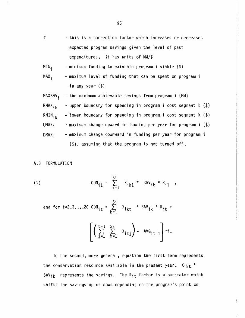
95
f - this is a correction factor which increases or decreases
expected program savings given the level of past
expenditures. It has units of MW/$
MINi -minimum funding to maintain program i viable ($)
MAXi - maximum level of funding that can be spent on program
i n any year ( $)
the maximum achievable savings from program i {MW)
- upper boundary for spending in program i cost segment
- 1 ower boundary for spending in program i cost segment
i
k
k
MAXSAV i
RMAXik
RMINi k
UMAXi - maximum change upward in funding per year for program i
DMAXi -maximum change downward in funding per year for program
($), assuming that the program is not turned off.
A.3 FORMULATION
( 1) Si
= L: k=l
Si and for t=2,3, ••• 20 CONit = L:
k=1
[( ~1 J=1
Sk L: k=1
In the second, more general, equation the first term represents
the conservation resource available in the present year. Xikt *
SAVik represents the savings. The Rit factor is a parameter which
shifts the savings up or down depending on the program's point on
($)
( $)
($)

96
the ramp. The second term acts to adjust conservation even more
with respect to the ramping concept. If prior resource allocations
for the program are less than what would be expected on average,
then a certain percentage, f, of the savings is subtracted. If more
resources have been acquired, the present year's estimate is
increased. The total conservation due to program i in year t is
therefore:
t-1 ~ d; t-J· * CON;J· + CONit j=l
where the d; t-j depreciates the savings.
This type of term must be included in the constraint that sets
demands equal to resources. One term must be specified for each
year in the planning period.
(2) This constraint puts a limit on the amount of conservation
attainable from program i. The depreciation factor has been left
out.
20 ~ CONit ~ MAXSAV; t=l
(3) This constraint sets a minimum viable program i funding level.
One constraint is needed for each year.
Si ~ k=l
on X > MIN *X ikt- i it
Explanation -the right-hand side will be zero if the program is turned off; the right-hand side will equal MIN; if the program is on.
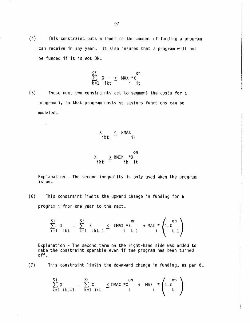
97
(4} This constraint puts a limit on the amount of funding a program
can receive in any year. It also insures that a program will not
be funded if it is not ON.
Si on L X < MAX *X k=1 ikt i it
(5} These next two constraints act to segment the costs for a
program i, so that program costs vs savings functions can be
modeled.
X < RMAX ikt ik
on X > RMIN *X ikt ik it
Explanation - The second inequality is only used when the program is on.
(6} This constraint limits the upward change in funding for a
program i from one year to the next.
Si L X k=1 ikt
Si - L:
k=1
on X < UMAX *X i kt-1 i t-1
+MAX* (1-X0
n ) i t-1
Explanation - The second term on the right-hand side was added to make the constraint operable even if the program has been turned off.
(7) This constraint limits the downward change in funding, as per 6.
Si ,Ex k=1 ikt-1
Si - 2:: X
k=1 i kt
on < DMAX *X
t

( 8)
98
These are consistency constraints.
(a) X > 0 -ikt
on t on t off {b) X = I: y I: y > 0
it j=l ij j=1 ij
20 on (c) I: y < 1 -j=1 ij
on off y y = 0 or 1 for all ij ij i = 1,2, ••• P
j = 1,2, ••• 20
on on Constraint (b) defines X in terms of the binary variables y
' it ij off
Y.. When coupled with (c), this allows a program to be turned on lJ
and off only once during the planning period. This could easily be
changed to allow programs to be turned off and on multiple times if
that seemed to model the situation more appropriately.
(9) This constraint insures that funding will be spread across a
minimum number of programs.
P on L X > PORT i=1 it t
The objective function would include
START· yon) 1 it
99
as the cost of conservation. The start up costs could be omitted
here and incorporated into operating costs.
While the current model uses binary variables to turn programs on
and off, thus creating a mixed integer formulation, this could be relaxed on
to allow the LP to choose the implementation rate by letting Xit take on
values between 0 and 1. While this would provide an LP representation,
the appropriateness of the modeling requires further study.
Uncertainty could be handled by the techniques described in
Sect. 7 .3 of this report.
A.4 DISCUSSION
Several efforts would need to be undertaken to provide the capabi-
lity to model individual conservation programs. A general view of the
factors affecting conservation and an understanding of the typical rela
tionship between them seems to be a first step. Figures A.l and A.2
represent an attempt to begin this process. A "toolbox" of formulations
for the standard relationships encountered between the factors would
a 1 so be necessary.
In fact, it may be possible to automate the model building task to
allow planners to answer a series of questions, possibly generated by a
microcomputer, and then to produce the corresponding constraints for an
LP implementation. With the availability of microcomputer based LP
software these models could be tested against various demand patterns
and the planner could determine whether the model adequately reflects
the important aspects of the conservation program. Several outputs,
including graphics, would need to be produced and studied to understand
the reaction of the model to the various demand patterns. The graphs
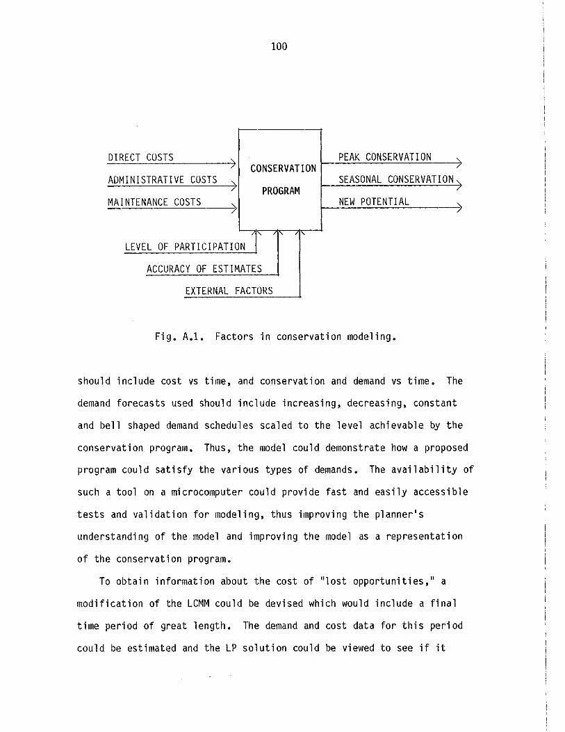
100
DIRECT COSTS ' PEAK CONSERVATION / CONSERVATION
ADMINISTRATIVE COSTS ?
SEASONAL CONSERVATION PROGRAM
MAINTENANCE COSTS ?
NEW POTENTIAL
LEVEL OF PARTICIPATION 'I' /
ACCURACY OF ESTIMATES
EXTERNAL FACTORS
Fig. A.l. Factors in conservation modeling.
should include cost vs time, and conservation and demand vs time. The
demand forecasts used should include increasing, decreasing, constant
and bell shaped demand schedules scaled to the level achievable by the
conservation program. Thus, the model could demonstrate how a proposed
program could satisfy the various types of demands. The availability of
such a tool on a microcomputer could provide fast and easily accessible
tests and validation for modeling, thus improving the planner's
understanding of the model and improving the model as a representation
of the conservation program.
To obtain information about the cost of "lost opportunities," a
modification of the LCMM could be devised which would include a final
time period of great length. The demand and cost data for this period
could be estimated and the LP solution could be viewed to see if it

101
significantly affected the proposed solution. This "infinite horizon"
plan could possibly point out missed opportunities which would not
appear in the 20-year plan. The current implementation may discourage
plans to obtain conservation in the latter years of the planning
hori zan.
DIRECT COSTS ADMINISTRATIVE COSTS
~AINIENANCE GUSTS
LEVEL OF PARTICIPATION P CCURACY OF ESTIMATES
EXTERNAL FACTORS
PEAK CUNSERVATIUN SEASONAL CONSERVAIIUN
NEW POTENTIAL
DIRtCT COSIS 1 1 -1
ADMINISTRATIVE COSTS ( • . 1 c 1'11\l N I tNANCE GUS I l 1 • 1 1
LEVEL OF PARTICIPATION * -1
"CcURACY UF ESTIMATES c • -1 • l eXTERNAL 1-ACTURS
PEAK CONSERVATION • • StASUNAL CONSERVATION • • • NEW POTENTIAL • l L
LEGEND
+ FACTOR ON LEFT INCREASES FACTOR ON TOP DIRECTLY - FACTOR ON LEFT DECREASES FACTOR ON TOP DIRECTLY ? FACTOR ON LEFT INFLUENCES FACTOR ON TOP IN UNDETERMINED MANNER 0 FACTOR N LEFT DOES NOT AFFECT FACTOR ON TOP DIRECTLY * SAME FACTOR OR NO LOGICAL RELATIONSHIP BETWEEN FACTORS
Fig. A.2. Relationship between conservation modeling factors.
102
It is important to remember when judging the complexity of LP for
mulation that the number of inequalities and the number of variables are
the important factors. Almost all of the equalities used in describing
the models are of the "bookkeeping" variety and should not be present in
the internal representation submitted to the optimization routine.
Upper and lower bounds can be handled by special techniques and are,
therefore, not added into the inequality count.
The formulation of the problem seems to be such that a decomposition
algorithm, such as Dantzig-Wolfe, could be used to solve the LP by
solving the subproblems associated with each of the resource groups and
combining those solutions through the coordination of a master problem,
based on the demand constraints, to produce a solution to the full LP.
Decomposing the problem allows the algorithm to solve several small
problems instead of one very large problem, and this usually results in
substantial savings of time in computation. In most decomposition
algorithms, prices for resources are generated by the algorithm as a
means of coordinating the solutions of subproblems. These prices could
be considered as internal transfer prices or measures of the subsidizing
of one resource by another. These prices, which are a by-product of the
solution, could be a useful tool in understanding how the resource
groups interact to satisfy demand.
With the increasing speed of mathematical programming algorithms
and the emergence of new techniques for optimization, keeping the model
small should not be the major concern. Obtaining a reasonable model of
the factors affecting the decision to be made and their relationships is
most important.
103
APPENDIX B
NOTE ON RESIDENTIAL SECTOR BASE HOUSES
B.1 INTRODUCTION
This Appendix addresses the issue of base house specification in
conservation planning and power forecasting. Summarized are how the
Office of Conservation and the Division of Power Forecasting specify
base houses in their respective analyses. These presentations are
followed by a discussion of the differences between the two approaches
and the consequences thereof to the integrity of the conservation
planning process.
B.2 RESIDENTIAL BASE HOUSES USED IN CONSERVATION PLANNING
The Office of Conservation has a set of standard assumptions con
cerning the characteristics of base houses (Scanlon, 1984). Several
assumptions are identical across Conservation's set of six base houses.
Some of these assumptions are that the house is ranch style, has wood
frame construction, and has 1350 square feet. These assumptions are
identical for houses found in the three climate zones (represented by
the cities of Portland, Spokane, and Missoula) and six configurations of
base house conservation characteristics.
The six types of base houses are listed in Table B.1 and are typical
existing, full weatherization existing, typical new, and Model
Conservation Standard New Housing for each climate zone. Each of the
base houses is used to determine conservation potentials for input into
the supply curves. For example, if X existing units have only R-11 in
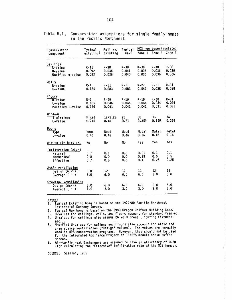
104
Table B.l. Conservation assumptions for single family homes in the Pacific Northwest
Conservation Typical Full wx. Typic~l MCS new suQerinsulated component existing! existing new Zone 1 Zone 2 Zone 3
Ceilings R-value R-11 R-38 R-30 R-38 R-38 R-38 U-value 0.092 0.036 0.041 0.036 0.036 0.036 Modified u-value 0.083 0.036 0.040 0.036 0.036 0.036
Walls --""lr-value R-4 R-11 R-11 R-27 R-31 R-31
U-value 0.124 0.083 0.083 0.042 0.038 0.038
Floors -r-Yalue R-2 R-19 R-19 R-19 R-30 R-31
U-va 1 ue 0.165 0.046 0.046 0.046 0.034 0.034 Modified u-value 0.116 0.041 0.041 0.041 0.031 0.031
Windows I glazings Mixed 1G+S,2G 2G 3G 3G 3G u-value 0.746 0.46 0.71 o. 359 0. 359 0.359
Doors --,ype Wood Wood Wood Metal Metal Metal
U-value 0.46 0.46 0.46 0.16 0.16 0.16
Air-to-air heat ex. No No No Yes Yes Yes
Infiltration (AC/H) Natural 0.7 o. 6 0.6 0.31 0.1 0.1 Mechanical 0.0 o.o 0.0 0.29 0.5 0.5 Effective 0.7 0.6 0.6 0.4 0.25 0.25
Attic ventilation Des1gn (Ac/H) 6.0 12 12 12 12 12 Average ( u ) 3.0 6.0 6.0 6.0 6.0 6.0
CrawlsQ. ventilation Design (Ac/H) 3.0 6. 0 6. 0 6.0 6. 0 6.0 Average ( " ) 1.5 3.0 3.0 3.0 3. 0 3.0
Notes: r:--Typical Existing home is based on the 1979/80 Pacific Northwest
Residential Economy Survey. 2. Typical New home is based on the 1980 Oregon Uniform Building Code. 3. U-values for ceilings, walls, and floors account for standard framing. 4. U-values for ceilings also assume 2% void areas (lighting fixtures,
etc.). 5. Modified U-values for celings and floors also account for attic and
crawlspasce ventiliation ("Design" values). The values are normally used in SPA conservation programs. However, they should not be used for the Integrated Appliance Project if TRNSYS models these buffer spaces.
6. Air-to-Air Heat Exchangers are assumed to have an efficiency of 0.70 (for calculating the "Effective" infiltration rate of the MCS homes).
SOURCE: Scanlon, 1985

105
the ceilings, then adding more insulation to each of these homes could
result in Y energy savings per year. Data which flow to the Office of
Conservation about the number of existing unweatherized and weatherized
and new single family homes for each year in the 20-year planning period
are used with energy saving estimates for measures to fully specify the
conservation supply curves.
B.3 RESIDENTIAL BASE HOUSES USED IN POWER FORECASTING
The specification of base houses in residential power forecasting is
more complex than in conservation planning. Essentially, base house
assumptions in power forecasting are made with respect to the structure
of the residential energy demand model, available data, and policy con
siderations that the model must address. This section begins by pre
senting a short discussion about the residental model. Next, parameters
for the model's base house are presented. The balance of the subsection
describes how these parameters were determined.
The most important feature of the residential model that pertains to
base house analysis is that the model does not represent explicitly base
house characteristics. That is, the accounting features of the model do
not specify a base house as containing Rll in the walls, Rll in the
ceiling, etc. Instead, the base house is represented as a point on an
efficiency curve, where 1.0 is the efficiency of the base house. The
base house energy use times an efficiency factor yields energy use for
houses that may be more or less efficient than the base house.
The characteristics of the base house in the residential model can
be "backed out" following a complex process. This process, described
below, yielded the following results: the base house has 1350 sq ft and
106
has less energy use than a house with Rll in the walls, Rl9 in the
ceiling, Rll in the floors, R2 in the doors, single glazing and 0,6 air
changes/hour but more than a house with Rl1 in the walls, R30 in the
ceiling, R11 in the floors, R2 in the doors, double glazing and 0,6 air
changes/hour.
This base house compares favorably with an interpolation of a base
house between the typical existing and typical new base houses used by
the Office of Conservation (Table B.1}. The base house in the residen
tial energy demand model is tighter than the typical existing house
(more wall, ceiling, and floor insulation and less air infiltrations)
and slightly less tight than the typical new house (less floor
insulation).
The process of how these characteristics were arrived at is very
interesting. The process is structured around three base house specifi
cations, a prototypical house that represents existing houses in the
region, a building standards in place house for primarily late model
houses, and a model council standards house. The residential base house
specification process begins its calculations with specifications for
three prototypical houses, one for each climate zone, found in Palmiter
and Baylin (1982}. All three of these houses are specified at 1350 sq
ft, just like the Office of Conservation houses.
The data provided for each house represent a series of 12 points
that pertain to various levels of energy efficiency and the costs of
acquiring the efficiency improvements. For example, point one repre
sents the typical existing house without any weatherization. The second
point may represent a house with additional ceiling insulation. The
third house would also include increased wall insulation. The twelfth

107
house has a maximum efficiency, Computer programs associated with the
residential energy demand model transform these data in several ways.
First, each 12-point distribution is interpolated to 16 points. This is
done to facilitate aggregating the three bases houses into one 16-point
distribution to represent a technical efficiency curve for only one base
house. After the interpolations are done, the aggregation is done.
The third step involves fitting a three-parameter curve to represent
this curve. The curve fitting routine weights the points closest to
point 1 heavier than for points closest to point 16 under the assumption
that near-term housing efficiency improvements will represent activities
nearer the top of the curve.
After the curve is fit, the curve is rebased. The old curve has at
point 1.0 the aggregated prototypical house. Efficiency of 0.9 would
represent a more efficient house. The curve is rebased so that 1.0
corresponds to the building standards in place house. This means that
the aggregated prototypical house would have an efficiency of greater
than 1.0. The house corresponding to the rebased 1.0 efficiency is the
model's new base house. By going back to the original aggregated curve
and determining the efficiency of the new base house from the curve, it
was possible to approximate the characteristics of the new base house
given above.
B.4 DISCUSSION
Three points must be made with respect to base house specification.
First, the current base house specifications are fairly similar. No
major inconsistency exists at this time. Second, achieving perfect con
sistency between Office of Conservation and Division of Power Forecasting

108
base houses may be practically impossible given the nature of the resi
dential model. The model can only utilize one base house and the tech
nical efficiency curves are not measure specific. "Backing out"
measures is possible, but the lumpiness of measures vs the continuity
of curves basically ensures that the backout procedure will never yield
a perfect fit.
Third, Power Forecasting has to develop base houses with respect to
all energy types, whereas Conservation base houses only have to relate
to houses with electric heat as a space heating fuel. In the future,
Conservation may specify base houses by subregion and signer-nonsigner
utilities. These observations suggest that base house specification
between the groups need not be identical with each other, just con
sistent with the goals of the analysis.

1. 2. 3. 4. 5. 6. 7. 8. 9.
10. 11. 12.
l 09 ORNL/CON-190
INTERNAL DISTRIBUTION
R. B. Braid 13. L. McCold M. A. Brown 14. J. W. Michel R. s. Carlsmith 15. R. w. Mixon J. Christian 16. D. c. Parzyck G. A. Dailey 17. J. H. Reed w. Fulkerson 18. R. B. Shelton D. Hamb 1 in 19. T. J. Wilbanks E. Hirst 20. Central Research Library R. B. Honea 21. Document Reference Section L. Jung 22. Laboratory Records (RC} M. P. Kertesz 23-24. Laboratory Records Dept. J. M. MacDonald 25. ORNL Patent Section
EXTERNAL DISTRIBUTION
26. Institute for Energy Analysis, ORAU-Library 27. Office of Assistant Manager for Energy Research and
Development, DOE-ORO. 28-54. Technical Information Center, DOE, P. 0. Box 62, Oak Ridge,
Tennessee 37831. 55-600. External Decision Systems Research Section Distribution
Mailing List and Extra Copies toM. s. Hubbard, 4500N, H-32.