o l . 7, is s u e 1, no v 2017 issn : 2249-5762 (online ... surface stresses result: ... and cut...

IJRMET Vol. 7, IssuE 1, NoV 2016 - ApRIl 2017 ISSN : 2249-5762 (Online) | ISSN : 2249-5770 (Print)

w w w . i j r m e t . c o m 60 INterNatIONal JOurNal Of reSearch IN MechaNIcal eNgINeerINg & techNOlOgy

Optimization of Locomotive Wheel by Using Finite Element Technique

1K. Chaitanya, 2L. Abhilash1,2Dept. of Mechanical Engg., Sree Vani Group of Education Society, Krishna (dist), AP, India

AbstractDamage mechanisms such as surface cracks, plastic deformation and wear can significantly reduce the service life of rolling stock. They also have a negative impact on the rolling noise as well as on the riding comfort. A proper understanding of these mechanisms requires a detailed knowledge of physical structure and specifications of wheel.New specifications are being imposed on railway wheel wear and reliability to increase the time between wheel re-profiling operations, improve safety and reduce total wheel set lifecycle costs. In parallel with these requirements, changes in railway vehicle missions are also occurring. These have led to the need to: operate rolling stock on track with low as well as high radius curves; increase speeds and axle loads and contend with a decrease in track quality due to a reduction in maintenance. These changes are leading to an increase in the severity of the wheel/rail contact conditions.So there is a need to optimize the wheel through several considerations such as material properties, shape, design features etc. The shape optimization is done by preparing a model in pro-e and analysis in Ansys.

KeywordsLocomotive Wheel, Finite Element Technique, PRO-E, ANSYS

I. IntroductionIndian railway, the prime movers of the nation, has the distinction of being one of the largest railway systems in the world under a single management. Its contribution to the nation’s progress is immeasurable and it has a dual role to play as a commercial organization as well as a vehicle for fulfillment of aspiration of the society at large.During the last decades substantial progress has been made in the design of railway vehicles and running gear. Tilting trains, high speed trains, active steering wheel sets and other sophisticated solutions have been introduced. In spite of this progress, the mechanics of a railway wheel set remains unchanged and an inappropriate combination of wheel and rail profiles can easily undermine these technological advances. Besides, older equipment has a special need for appropriate combinations of wheel/rail profiles as they do not have high-tech devices that improve their performance. The design of a wheel profile is an old problem and various approaches were developed to obtain a satisfactory combination of wheel and rail profiles. Usually, it is possible to find an optimal combination when dealing with a closed railway system, i.e. when only one type of rolling stock is running on a track and no influence of other types of railway vehicles is present.

II. Wheel

A. Wheel ArrangementsModern Diesel and Electric Locomotives Starting with modern equipment and the usual method of describing how the driving

and non-driving (carrying or trailing) wheels are distributed under a locomotive; there are two simple basic rules. First, the wheels are not individually identified, only the axles and, second, trailing wheels are allocated numbers and driving wheels are allocated letters. The letter or number refers to the number of axles in a single frame, for example:

Fig. 1: Older Designs

B. Types of Wheels

Specification (mm)

Solid wheel for passenger car

915 C - 915 D 950 -1092

Solid wheel for freight car 840B - 840C 840D - 840E

Whole processing wheel for passenger car

915D 915D (S-type) 950 (international true train)

Solid wheel for metallurgical rolling stocks 840 thick web

Rough wheel tyre for locomotive 846 – 1756

IJRMET Vol. 7, IssuE 1, NoV 2016 - ApRIl 2017

w w w . i j r m e t . c o m INterNatIONal JOurNal Of reSearch IN MechaNIcal eNgINeerINg & techNOlOgy 61

ISSN : 2249-5762 (Online) | ISSN : 2249-5770 (Print)

Rough wheel tyre for electric locomotive 606 – 686

High quality carbon steel rolled civil ring

Outer diameter 600 -2010 (ring, max 2500) inner diameter >500 thickness 50 - 160 height 70 - 200 weight 100 -970 kg.

Alloy structure steel rolled civil ringHigh quality carbon steel hot rolled civil ring50 Mn gear ring for truck crane50SiMn grinding ring for milling pit35SiMn grinding ring for petroleum mechanism

C. Designation OF INDIAN locomotivesLocos, except for older steam ones, have classification codes that identify them. This code is of the form ‘[gauge][power][load][series][subtype][suffix]’In this the first item, ‘[gauge]’, is a single letter identifying the gauge the loco runs on:

W = Broad GaugeY = Meter GaugeZ = Narrow Gauge (2’ 6”)N = Narrow Gauge (2’)The second item, ‘[power]’, is one or two letters identifying the power source:D = DieselC = DC tractionA = AC tractionCA = Dual-power AC/DC tractionB = Battery electric (rare)The third item, ‘[load]’, is a single letter identifying the kind of load the loco is normally used for:M = Mixed TrafficP = PassengerG = GoodsS = ShuntingL = Light Duty (Light Passenger?) (No longer in use)U = Multiple Unit (EMU / DEMU)R = Railcar

D. Wheel Profile

Fig. 2: Worn and Unworn Wheels

Cast steel wheels originated in United States, use of the approved wheel is began in 1965. By 1974 Cast Wheels where incorporated into the Canadian Specification (UIC). Rapid acceptance and use has resulted in cast steel wheels comprising 90% of North American Wheel Market. Cast Wheel yield reduced traction on effort to the magnitude of 5~70%. North America is joined by Mexico, Canada, India & South America in using Cast Steel Wheels.

III. Wheel DefectsRailway operations need to ensure safety reliability Railway wheels are safety critical Components regularly monitored re-profiled as needed is costly causes operational disturbances ensures safe operations need to classify wheels to ensure optimal reprofiling intervals

A. Wheel damage –IndentationsGravel (or other objects) is trapped between the wheel and the rail typically results in smooth pits that are benign (no further crack growth)

Fig. 3: Wheel Damage –Indentations



B. Wheel Damage –WearWear occurs from sliding between the wheel and rail, typically in the flange root area Benign (slow process).Too high wear is monitored by geometry measurements

Fig. 4: Wheel Damage –Wear

C. Wheel Damage –Wheel FlatsFormed by a locked wheel sliding on a rail Part of the wheel becomes flattened, Thermal damage (and marten site) may form at the flat Causes high impact loads that may result in cracking, noise and discomfort

Fig. 5: Wheel Damage –Wheel Flats

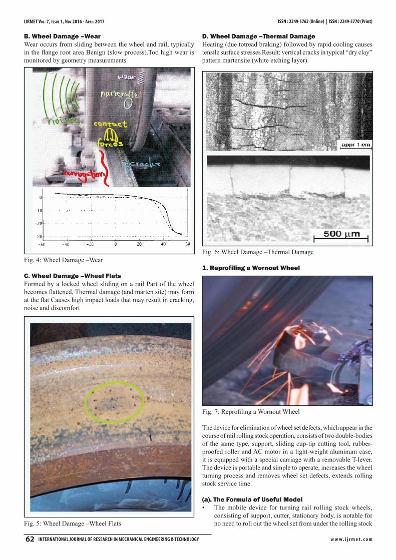
D. Wheel Damage –Thermal Damage Heating (due totread braking) followed by rapid cooling causes tensile surface stresses Result: vertical cracks in typical “dry clay” pattern martensite (white etching layer).

Fig. 6: Wheel Damage –Thermal Damage

1. Reprofiling a Wornout Wheel

Fig. 7: Reprofiling a Wornout Wheel

The device for elimination of wheel set defects, which appear in the course of rail rolling stock operation, consists of two double-bodies of the same type, support, sliding cup-tip cutting tool, rubber-proofed roller and AC motor in a light-weight aluminum case, it is equipped with a special carriage with a removable T-lever. The device is portable and simple to operate, increases the wheel turning process and removes wheel set defects, extends rolling stock service time.

(a). The Formula of Useful Model The mobile device for turning rail rolling stock wheels, • consisting of support, cutter, stationary body, is notable for no need to roll out the wheel set from under the rolling stock




as the wheel set is turned due to application of the portable body, actuator and jacks.The device described in p.1. is notable for use of locomotive • battery as a power supply for wheel turning.

(b). Summary Mobile device for turning rail rolling stock wheels. It is applied for elimination of wheel defects, which appear while in service. Assignment - extension of wheel service time, reduction of rolling stock out-of-service time.Technical result - elimination of sharp flange, reduced flange in case of wear and resurfacing.The defects are eliminated without rolling wheel sets out from under the loaded rolling stock, which reduces delay time and improves traffic safety.The device consists of a portable body, support, actuator, rheostat, power supply and two jacks.

B. Testing A Locomotive

Fig. 8:

A DYNAMOMETER CAR, attached between the locomotive and the train, is used for making tests under working conditions. This coach is 48 ft. 5 in. long and weighs 27 tons 3 cwt. In the car a moving roll of paper, on which the principal records are made, is operated by clockwork and the extra wheel shown. This can be raised or lowered from the underside of the carriage to the rail as required, and is used to record on the roll the speed at which the train is travelling. The wheel is fitted with a hardened steel tyre, ground to such a diameter that it makes exactly 440 revolutions for each mile run.

Fig. 9:

ON TEST. The “Cock o’ the North,” the great L.N.E.R. 2-8-2 locomotives, in the testing shop at Vitry, France. The engine, without the tender, is held securely at the rear, with the wheels resting on rollers. Steam is raised in the boiler, and all quantities of water and fuel used are carefully measured. The locomotive regulator is opened and the wheels cause the supporting rollers to revolve. The rollers are coupled to paddle wheels inside the

water drums shown at the left of the picture. The churning action of the paddles absorbs the power of the engine and provides a load which can be varied and measured at will.

Fig. 10:

WHEEL BALANCING, an important part of a locomotive’s testing which is carried out during construction. This machine, at Swindon locomotive works, is used to ensure that all engine driving wheels shall be capable of spinning without undue vibration, at a speed equivalent to over sixty miles an hour on the track.

IV. PRO-E

A. IntroductionAs the world’s one of the supplier of software, specifically intended to support a totally Integrated product and development process Parametric Technology Corporation (PTC). Is recognized as a strategic partner, which can help a manufacturer to turn a process .Into competitive advance, greater market share and higher profits and an industrial and mechanical design to functional simulation manufacturing and information management. Fully associated PRO/E solutions encompass all aspects of the development cycle and cut design time by half, improve product quality and ensure a team’s success .PRO/E Mechanical design solutions will improve our design productivity allowing us to finish more complex and challenging projects in less time. Leading companies around the world have standardized on PRO/E to help their design team meet today’s most aggressive design objective .To help to meet these challenges, parametric technology has created the most comprehensive, integrated project product development environment available today. PTC’s mechanical design solutions deliver all the tools we need to transform the product development process into a strategic competitive advantage for any company. The key in developing higher quality products in less time depends on our ability to quickly and accurately model the entire product and easily incorporate important changes to any point in the design process. Changes occurring late in the design cycle are responsible to increased cost over runs and missed deadlines. As a result many changes that improve the design are never implemented. PRO/E mechanical design solutions deliver the technological edge we need to complete quickly and still respond to last minute changes. In addition PRO/E ensures that all downstream deliverables be automatically updated to reflect the final design, dramatically reducing costs and delays. Now our design can meet or exceed its development targets for schedule, budget and quality.

B. Modules in PRO/EThere are mainly different modules in Pro/E using which we can perform different tasks. Following are the important modules of Pro/E.



1. Sketcher Module Sketcher module enables us to create sections. Sketcher techniques are used in many areas of pro/E. Using sketcher mode, we create geometry without regard to the exact relationships between parts of the sketch or the exact values of the dimensions, when we generate the sections. Pro/E makes explicit assumptions. For example if you draw nearly horizontal line, it becomes exactly horizontal, and all these assumptions are displayed graphically

2. Part ModuleThis starts by adding a set of default datum planes and creating the first solid and surface features, then continued to add to achieve the design shape by creating various construction features are protrusions, slots and cuts, holes, shafts, chamfers, ribs, shells, pipes etc.

3. Advanced Part ModuleUsing conventional cad systems mainly uses this module to create complex 3-d images that are otherwise difficult to create. It mainly includes features like sweep, blend, helical sweep and variable sections blends etc.

4. Drawing ModuleDrawing mode, available with basic pro/E provides us with the basics functionally to document our solid models are surface models. Drawings share a two-way associatively with the model. When we make changes to the model in part or assembly mode, the system automatically updates and reflects the changes, like

wise, any changes that we make to the model in drawing mode become immediately visible on the model in other modes. We can use basic pro/e to create drawing views of one or more models in several standard view types and dimension them.

5. AssemblyFew designs consist of just single part. Most designs are combinations of several thousands of parts .An assembly drawing for documentation is traditionally a Multi-view drawing of the complete design showing each, component in its relative position and identified by name. Generally overall dimensions are shown in the assembly drawing. For more complex design, the assembly is divided into functional subassemblies, which are identified in the assembly drawing. Individual components are then identified at the subassembly level. Assembly shows all parts both standard and non standard a standard part is one, which we3 simply purchase from manufacturer and use as it is. A non standard or custom part is one we must design for the current project.

6. Detail ModuleIt extents the drawing capability offered by pro/E. We can use if with basic pro/E standalone module to create, view and annotate, models and drawings. Pro/E detail supports additional view types and multi sheets. It offers numerous commands for manipulating items in a drawing and enables us to add it to customize is engineering drawing with the geometry to create drawing formats and makes multiple cosmetic changes to drawings.

Fig. 10:




C. Modelling ProcedureModeling of wheel is done in pro-e (wild fire3). The procedure is as follows

First the half sectional view of the wheel profile is drawn 1. according to Indian railways standard dimensions using sketcher module.The half sectional sketch is rotated along a horizontal axis 2. using rotate option and part model is constructedPart model for wheel is constructed for both 1in20 and 1in15 3. taper on the wheel tread.

Fig. 11:

V. ANSYS

A. Introduction to ANSYSThe ansys computer program is a large scale multipurpose finite element program. Which may be used for solving several classes of engineering analyses. the analysis capabilities of ANSYS include the ability to solve static and dynamic structural analyses, steady state and transient heat transfer problems, mode frequency and buckling, Eigen value problems, static or time varying magnetic analyses and various types of field and coupled field applications. The program contains main special futures which allow nonlinearities or secondary effects to be include in the solution such as plasticity large strain, hyper elasticity, creep, swelling, large deflections, contact, stress stiffening, temperature dependency, material anisotropy and radiation. ANSYS has been developed.Other capabilities ,sub structuring, sub modeling, random vibration, kinetostastics, kinetodynamics, free convection, fluid analysis, acoustics, magnetics, piezoelectrics, coupled field analysis and design analysis and, design optimization have been added to the program. These capabilities contribute further to making ANSYS a multipurpose analysis tool for varied engineering disciplines.The ANSYS program has been in commercial use since 1970, and has been used extensively in the aerospace, automotive, construction, electronic, energy services, manufacturing, nuclear, plastics, oil, and steel industries. In addition, many consulting firms and hundreds of universities use ANSYS for analysis Research and educational use.

B. Definition of Structural AnalysisStructural analysis is probably the most common application of the finite element method. The term structural (or structure) implies not only civil engineering structures such as bridges and buildings, but also naval, aeronautical, and mechanical structures such as ship hulls, aircraft bodies, and machine housings, as well as mechanical components such as pistons, machine parts, and tools.

C. Types of Structural AnalysisThe seven types of structural analyses available in the ANSYS family of products are explained below. The primary unknowns (Nodal degrees of freedom) calculated in a structural analysis are displacements. Other quantities, such as strains, stresses, and reaction forces, are then derived from the nodal displacements. Structural analyses are available in the ANSYS/Metaphysics, ANSYS/Mechanical, ANSYS/Structural, and ANSYS/Linear Plus programs only. You can perform the following types of structural analyses: Static Analysis-Used to determine displacements, stresses, etc. under static loading conditions. Both linear and Non-linear static analysis. Nonlinearities can include plasticity, stress stiffening, large deflection, large strain, hyper elasticity, contact surfaces, and creep.

Modal Analysis-Used to calculate the natural frequencies and mode shapes of a structure. Different mode extraction methods are available. Harmonic Analysis-Used to determine the response of a structure to harmonically time-varying loads. Transient Dynamic Analysis-Used to determine the response of a structure to arbitrarily time-varying loads. All nonlinearities mentioned under Static Analysis above are allowed. Spectrum Analysis-An extension of the modal analysis, used to calculate stresses and strains due to a response spectrum or a PSD input (random vibrations Buckling Analysis-Used to calculate the buckling loads and determine the buckling mode shape. Both linear (Eigen value) buckling and nonlinear buckling analyses are possible.

D. Uses of Modal AnalysisYou use modal analysis to determine the natural frequencies and mode shapes of a structure. The natural frequencies and mode shapes are important parameters in the design of a structure for dynamic loading conditions. They are also required if you want to do a spectrum analysis or a mode superposition harmonic or transient analysis. You can do modal analysis on a prestressed structure, such as a spinning turbine blade. Another useful feature is modal cyclic symmetry, which allows you to review the mode shapes of a cyclically symmetric structure by modeling just a sector of it. Modal analysis in the ANSYS family of products is a linear analysis. Any nonlinearity, such as plasticity and contact (gap) elements, are ignored even if they are defined. You can choose from several mode extraction methods: subspace, Block Lanczos, Power Dynamics, reduced, unsymmetrical, and damped. The damped method allows you to include damping in the structure. Details about mode extraction methods are covered later in this section

VI. Finite Element Method

A. IntroductionThe Finite Element Method has become a powerful tool for the



numerical analysis technique for obtaining approximate solutions of a wide range of engineering problems. Because of its diversity and flexibility as an analysis tool, it is receiving much attention in engineering schools and industries. In more and more engineering situations, we find that it is necessary to obtain approximate solutions to problems rather than exact closed from solution. It is not possible to obtain analytical mathematical solutions for any engineering problems. An analytical solution is a mathematical expression that gives the values of the desired unknown quantity at any location in the body, as consequence it is valid for infinite number of location in the body. For problems involving complex material properties and boundary conditions, the engineering study shifts towards numerical methods that provide approximate, but acceptable solutions.

The finite element method as become a powerful tool for the numerical solution of a wide range of engineering problems. it has developed simultaneously with the increasing use of the high-speed electronic digital computer and with the growing emphasis on numerical methods for engineering analysis.

The fundamental areas that have to be learn for the working capability of finite element method include:

Matrix algebra.• Solid mechanics.• variational methods• Computer skills.•

Matrix techniques are definitely most efficient and systematic way to handle algebra of finite element method. Basically matrix algebra provides a scheme by which a large number of equations can be stored and manipulated. Since vast majority of literature on finite element methods’ treat problem in structural mechanics. It is useful to consider the finite element procedure basically as a variational approach.

The term “finite element distinguishes the techniques from the use of infinitesimal “differential elements” used in calculus, differential equations. The method is also distinguished from finite differential equations, for which although the steps in to which space is divided in to finite elements are finite in size, there is a little freedom in the shapes that the discrete steps can take. FEA is a way to deal with the structure that are more complex than dealt with the analytically using the partial differential equations.

FEA deals with the complex boundaries better than finite differential equations and gives answers to the “real world “structural problems it has been substantially extended scope during the roughly forty years of its use.

FEA makes it possible to evaluate a details and complex structure, in a computer during the planning of the structure. The demonstration in the computer about the adequate strength of the structure and possibility of improving design during planning can justify the cost of these analysis works. FEA has also been known to increase the rating of the structures that work significantly over design and build many decades above.

B. Terms Commonly Used in FEMDescritization: The process of selecting only a certain number of discrete points on the body can be termed as descritization.

Continuum: The continuum is a physical body, structure or 1. solid being analyzed.Node: The finite elements, which are inter connected at joints, 2. are called nodes or nodal points Element: small geometrical regular figure are called 3. elements.Displays models: The simple functions, which are assumed 4. approximate the displacement for each element. These functions are called the displacements models or displacement functions. Local coordinate system: Local coordinate system is one 5. that is define for a particular element and not necessary for the entire body or structure.Global system: The coordinate system for the entire body is 6. called global system.Natural coordinate system: Natural coordinate system is a 7. local system, which permits the specification of points within the element by a set of dimension less numbers, whose magnitude never exceeds unity.Interpolation functions: It is a function, which has unit value 8. at one nodal point and a zero value at all other nodal pointsAccept ratio: The accept ratio describes the shapes of the 9. element in the assemblage for two dimensional elements these parameters is defined as the ratio of the largest dimension of the element to the smallest dimensionField variable: The principle unknowns of problems are called 10. the variables.

C. General Description of FEM In the finite element method, the actual continue of body matters like solid, liquids or gas is represented as an assemblage of sub divisions called finite elements. These elements are considered to be interconnected at specified points known as nodes or nodal points.These nodes usually lie on the element boundaries where an adjacent element is considered to be connected since the actual variations of the field variables(like displacement,stress,temperature, pressure and velocity) inside the continuum are is not known, we assume that the variation of the field variable inside a finite element can be approximated by a simple function. These approximating functions (also called interpolation models) are defined in terms of the values at the nodes when the field equations (like equilibrium equations) for the hole continuum are written, the new unknown will be the nodal values of the field variable. By solving the field equations, which are generally in the form the matrix equations the nodal values of the field variables will be known. Once these are known, the approximating function defines the field variable throughout the assemblage of elements.The solution of a general continuum by the finite element method always follows as a orderly step by step procedure for static structural problems can be stated as follow:

Step 1: Descritization of structure (domain)The first step in the finite element method is to divide the structural solution region into subdivisions or elements.

Step 2: Selection of proper interpolation model Since the displacement (field’s variable) solution of a complex structure under any specified load conditions can not be predicted exactly. We assume some suitable solution with in an element to approximate the solution. The assumed solution must be simple and it should satisfy certain convergence requirement.




Step 3: Derivation of element stiffness matrices and load vectors.From the displacement model the stiffness matrix [K(e)] and the load vector P(e) of element ‘e’ are to be derived by using the either equilibrium conditions are a suitable variational principle.

Step 4: Assemblage Stiffness of element to obtain the equilibrium equations:Step the structure is composed of several finite elements the individual element stiffness matrices and load vectors are to be assembled in a suitable manner the overall equilibrium equation as to be formulated

[K}Ф=PWhere [K] is called assembled matrix. Ф is called the vector of nodal displacement and P is the vector or nodal force complete structure.

Step 5: solution of system equation to find nodal values of displacement (field variable)The overall equilibrium equations have to be modified to account for the boundary conditions of the problem. After the incorporation of the boundary conditions, the equilibrium equations can be expressed as [K]Ф=PFor linear problems, the vector ‘Ф’ can be solved very easily. But for non linear problems, the solution has to be obtained in a sequence of steps, each step involving the modification of the stiffness [K] and Ф or the load vector P.

Step 6: computation of element strains and stresses.

D. Basic Approach to FEABasic approach for any finite element analysis can be divided into three parts:

Pre-processor• Solver• Post-processor•

1. Pre-processorPre-processor mainly contains building of model, meshing, assigning material properties etc.

(a). Building of ModelsGeometry is usually difficult to describe as it has to be as close as real. Since it has to take real world loads and boundary condition. It is equal to prototype simulated in a computer.

(b). Creation of Finite Element Model of MeshingAfter assigning material properties and structural properties to be model, meshing is done. Meshing means dividing a solid model in to a finite number of finite sized elements.

FEA uses a complex system of points called nodes, which make grid called MESH. This mesh is programmed to contain material and structural properties, which defined how the structure will react to certain loading conditions. Nodes are assigned at a certain density throughout the material depending on the anticipated stress levels of particular area. Reasons that will receive large amounts of stress usually have a higher node density than those when experience little or no stress.

Point of interest may consist of fracture point are previously tested material, fillets, corners, complex detail and high stress areas. The mesh acts like a spider web in that from each node. There extents a mesh element to each of the adjustments nodes. This web of vectors is what carries the materials properties to the object, creating many elements. Each finite element analysis programs may come with an element library or one is constructed over time. Elements are thought to fill the whole experiment hence choice of element is very critical.

While meshing it has to be decided whatever we have to go for finer mesh or coarser one. the finer the mesh ,the better will be the result but longer analysis time. Therefore, a compromise between accuracy and solution speed is usually made. The mesh may be created manually or automatically. In the manually created mesh, we will notice that the elements are smaller at joist. This is known as mesh refinement. And it enables the stress to be captured at the geometric discontinuities.

Manual meshing is a tedious process for models with any degree of complications, but inbuilt mesh engine creates mesh automatically thus reducing the time. These automatic meshing has limitations us to regards mesh quality and solution accuracy.

2. SolverSolvers are geometric task oriented. These are developed for specific applications. Solvers are designed based on continuum approach where in construction of mass, momentum and energy equations of stats, thermodynamic equation as and when required for each of the elements and solution is obtained by interpreting these solutions. The solution of these equations essentially depends on two methods:

Implicit1. Explicit2.

Choice of the method is based on the nature of the problems.The main goal pf a finite element analysis is to examine a structure or a component response to certain loading conditions. Therefore specifying the proper loading conditions is a key step in the analysis. These loading conditions may be static, dynamic or transient whose nature may be linear or non-linear.

The word loads in FEA includes the applied forcing functions externally or internally. For example, loads in structural are displacement, forces, pressures, temperatures and gravity. In thermal analysis the applied loads are temperature, heat flow rates convection and heat generation.

3. Post-ProcessorHere the results of the analysis are read and interpreted. They can be presented in the form of table, a contour plot. Deformed shape of the component or the node shapes and natural frequencies are involved. Other results are available for fluids, thermal and electrical analysis types. Contour plots are usually the effective way of viewing results for structural type problems. Slices can be made through 3-D models to facilitate the viewing of internal stress patterns.Post processor includes the calculation of stress and strains in any of the X, Y or Z directions or induced in a direction at an angle to the co-ordinate axes. The principal stresses and strains may also be plotted or if required the yield stress and strains according to the main theories of failure can be plotted.



VII. Optimization of Wheel Material

A. Introduction

Fig. 12:

Since the wheel is the main part, which is subjected to most vibrations and stresses, choice of the material should withstand these effects. Generally in India, plain carbon steels are used due to its low cost, excellent strength etc. Even though plain carbon steel has good properties, there is a need to introduce new materials to compete with advanced technology of other countries. New age always demands fast speed, riding comfort etc. so there is definitely a need of introducing new materials. As the speed increases, automatically vibrations increases and which in turn leads to more wearing in the wheels. To withstand these vibrations, alloy steels are proposed for the wheel material.Three materials are chosen for the wheel material and modal analysis is done using ANSYS

Materials chosen are:AISI 8640• AISI 1050• C50-PLAIN CARBON STEEL•

B. Porperties of the Materials

1. AISI 8640

Category Steel

Class Alloy steel

Type Standard

Common Names Nickel-chromium-molybdenum steel

Designations

Germany: DIN 1.6546 Italy: UNI 40 Ni Cr Mo 2 KB United Kingdom: B.S. Type 7 United States: ASTM A322, ASTM A331, ASTM A506, ASTM A519, MIL SPEC MIL-S-16974, SAE J404, SAE J412, SAE J770, UNS G86400

CompositionElement Weight %

C 0.38-0.43Mn 0.75-1.00 P 0.035 (max) S 0.04 (max) Si 0.15-0.30 Cr 0.40-0.60 Ni 0.40-0.70 Mo 0.15-0.25

Properties Conditions T (°C) Treatment

Density (×1000 kg/m3) 7.7-8.03 25 Poisson’s Ratio 0.27-0.30 25 Elastic Modulus (GPa) 190-210 25 Tensile Strength (Mpa) 1862

25

oil quenched, fine grained, tempered at 205°C more

Yield Strength (Mpa) 1669 Elongation (%) 10 Reduction in Area (%) 40

Hardness (HB) 505 25

oil quenched, fine grained, tempered at 205°C more

Mechanical Properties

AISI 1050Category SteelClass Carbon steelType Standard

Designations

Germany: DIN 1.1210 Japan: JIS S 53 C, JIS S 55 C United States: AMS 5085,AMS 5085A, ASTM A29, ASTM A510, ASTM A519, ASTM A576, ASTM A682, FED QQ-S-635 (C1050), FED QQ-S-700 (1050), MIL SPEC MIL-S-16974, SAE J403, SAE J412, SAE J414, UNS G10500


C 0.48-0.55 Mn 0.60-0.90 P 0.04 (max) S 0.05 (max)

Mechanical Properties


Density (×1000 kg/m3) 7.7-8.03 25

Poisson’s Ratio 0.27-0.30 25 Elastic Modulus(GPa) 190-210 25




Tensile Strength (Mpa) 636.0

25 annealed at 790°C more

Yield Strength (Mpa) 365.4

Elongation (%) 23.7 Reduction in Area (%) 39.9

Hardness (HB) 187 25 annealed at 790°C more

Impact Strength (J) (Izod) 16.9 25 annealed at

790°C more

C50-PLAIN CARBON STEEL

Chemical Composition (in weight %)C Si Mn Cr Mo Ni0.51 0.20 0.75 0.20 0.05 0.20

DescriptionC50 is a medium carbon steel is used when greater strength and hardness is desired than in the “as rolled” condition.

ApplicationsQuenched and subsequently tempered steel for screws, forgings, wheel tyres, shafts, sickles, axes, knives, wood working drills, hammers, etc. Physical properties (average values) at ambient temperature Modulus of elasticity [103 x N/mm2]: 205 Density [g/cm3]: 7.85 Specific heat capacity[J/g.K]: 0.48

Coefficient of Linear Thermal Expansion 10-6 oC-1

20-100oC 20-250oC 20-500oC11.5 13.0 14.0

Present Material used by Railway:

RWF manufactures cast steel wheels by a controlled pressure pouring process. In this process, the raw material used is pedigree scrap (old used wheel sets, axles etc, rejected as unfit for use by the Railways). The scrap steel is melted in Ultra High Frequency Electric Arc furnace. The correct chemistry of molten metal steel is established through a Spectrometer. The wheels are eventually

getting cast in the graphite moulds, which are pre-heated and sprayed. After allowing for a pre-determined setting time the mould is spilt and the risers are automatically separated from the cast wheel.


C 0.43-0.50 Mn 0.60-0.90 P 0.04 (max) S 0.05 (max)

Mechanical Properties:


Density (×1000 kg/m3) 7.7-8.03 25

Poisson’s Ratio 0.27-0.30 25 Elastic Modulus (GPa) 190-210 25

Tensile Strength (Mpa) 585

25

cold drawn, annealed (round bar (16-22 mm)) more

Yield Strength (Mpa) 505 Elongation (%) 12 Reduction in Area (%) 45

Hardness (HB) 170 25

cold drawn, annealed (round bar (19-32 mm)) more

Thermal Properties


Thermal Expansion (10-6/ºC) 15.1 0-700 more annealed

C. ANSYS ProgramModal analysis of the wheel is carried out on the wheel for 1. each of the above mentioned materials. Ansys is used for this analysis. The procedure is as follows…Preferences > structural > o.k2. Preprocessor > element type > add/edit/delete > tet 3. 10node92Material properties > isotropic > density , young’s modulus, 4. poisons ratio > o.kFile > import > IGES > o.k5. Meshing > size controls > global size > no. of element 6. divisions > o.kMesh tool > tet > mesh > select objects > o.k7. Solution > analysis type > new analysis > model > o.k8. Analysis options > no. of modes to extract. No. of modes to 9. expand > o.kSolution > solve current l.s10. General postproc > results summary > o.k 11. Modal analysis of the wheel is carried out on the wheel for 12. two different tapers on the wheel tread. 1in20 profile13.



1in15 profile14. Ansys is used for this analysis. The procedure is as 15. follows…Preferences > structural > o.k16. Preprocessor > element type > add/edit/delete > tet 17. 10node92Material properties > isotropic > density , young’s modulus, 18. poisons ratio > o.kFile > import > IGES > o.k19. Meshing > size controls > global size > no. of element 20. divisions > o.kMesh tool > tet > mesh > select objects > o.k21. Solution > analysis type > new analysis > model > o.k22. Analysis options > no. of modes to extract. No. of modes to 23. expand > o.kSolution > solve current l.s24. General postproc > results summary > o.k 25.

VIII. ResultsTable 1: Results for AISI 8640

SET TIME/FREQ LOAD STEP

SUBSTEP CUMULATIVE

1 317.07 1 1 1 2 317.40 1 2 2 3 392.43 1 3 3

Results for set 1

Results for set 2

Results for set 3

Table 2: Results for 1050

SET TIME/FREQ

LOAD STEP SUBSTEP CUMULATIVE

1 319.84 1 1 1 2 320.17 1 2 2 3 395.98 1 3 3

Results for set 1

Results for set 2




Results for set 3

Table 3: results for PLAIN CARBON STEEL (C50)

SET TIME/FREQ


1 320.617 1 1 1

2 320.967 1 2 2

3 407.989 1 3 3

Results for set 1

Results for set 2

Results for set 3

Table 4: results for PLAIN CARBON STEEL (C50)[ 1in15]

SET TIME/FREQ


1 115.75 1 1 1 2 116.41 1 2 2 3 211.35 1 3 3

Results for set 1

Results for set 2



Results for set 3

Table 5: Results for STEEL

SET TIME/FREQ


1 325.617 1 1 1 2 326.467 1 2 2 3 450.767 1 3 3

Results for set 1

Results for set 2

Results for set 3:

IX. ConclusionsWe had done the model analysis for three types of materials 1. for the profile 1in20 model.The frequencies obtained for the material AISI 8640 are less 2. when compared to other two materials.Therefore AISI 8640 can be preferred as a material for the 3. railway wheel.Due to its high cost and other factors, it is not being used by 4. Indian railways.Presently the Indian railways are using the rolled steel which 5. having more frequency than the plain carbon steel.So plain carbon steel is preferred to use by Indian railways.6. Frequencies are considerably reduced for 1in15 model. 7.

X. Scope for Future WorkThere is a need for replacing traditional plain carbon steel with 1. alloy steel, which will reduce wear rate up to some extent.Study for better and economic alloy steels is needed to 2. improve wheel life.Also study should be conducted in wheel profile for increasing 3. the wheel life.Research should be concentrated on wheel tread taper, since 4. it is the part which will be always in contact with rail.

Koppula Chaitanya, Studied B.Tech in Sree Kavitha Institute of Science and Technology (JNTU-H), and pursuing M.Tech ( Machine Design ) in Sree Vani School of Engineering(JNTU-K).

Lagada Pati Abhilash. Studied B.Tech in Sai Spurthi (JNTU-H), and Working as Asst Professor in Sree Vani School of Engineering (JNTU-K)

o l . 7, is s u e 1, no v 2017 issn : 2249-5762 (online ... surface stresses result: ... and cut...

Documents