nwp saf · marie doutriaux-boucher, loa, ... (have copy of .ppt) ... an eye on met-6 winds and...

NWP SAF Satellite Application Facility for Numerical Weather Prediction

Document NWPSAF-MO-VS-016

Version 1.3

12 September 2005 Visit to EUMETSAT to discuss AMVs (26-29 June 2005) Mary Forsythe1 and Marie Doutriaux-Boucher2 1Met Office, UK 2LOA University of Lille 1, France

NWP SAF

Visit to EUMETSAT to discuss AMVs

Doc ID : NWPSAF-MO-VS-016 Version : 1.3 Date :12/09/05

2

Visit to EUMETSAT to discuss AMVs (26-29 June 2005)

Mary Forsythe, Met Office, UK Marie Doutriaux-Boucher, LOA, University of Lille 1, France

This documentation was developed within the context of the EUMETSAT Satellite Application Facility on Numerical Weather Prediction (NWP SAF), under the Cooperation Agreement dated 16 December, 2003, between EUMETSAT and the Met Office, UK, by one or more partners within the NWP SAF. The partners in the NWP SAF are the Met Office, ECMWF, KNMI and Météo France. Copyright 2004, EUMETSAT, All Rights Reserved.

Change record Version Date Author / changed by Remarks

1.1 22/08/05 Mary Forsythe / Marie Doutriaux-Boucher

First Version

1.2 02/09/05 Mary Forsythe Minor amendments 1.3 12/09/05 Mary Forsythe Adding paragraph from ECMWF

NWP SAF



3

1. Introduction The main reason for visiting EUMETSAT was to discuss and investigate some of the problem areas for satellite winds (or atmospheric motion vectors, AMVs as they are also known) that were highlighted by the NWP SAF monitoring and cloud top pressure investigations. Additionally the visit provided a useful opportunity for sharing experience and knowledge with the new ECMWF satellite wind fellow, Claire Delsol. Our time was divided between looking at wind cases using EUMETSAT’s monitoring system and more formal meetings. The trip was very useful and has provided some explanations for our monitoring results and thrown up other ideas for improvement, both at EUMETSAT and within NWP. We plan to continue discussions via e-mail and arrange further meetings as necessary. We have recently participated in a visit to ECMWF to discuss the NWP approach in more detail. 2. Agenda Monday 27 June 2005 AM :

• MTP operations overview, check of some MTP wind products PM :

• MSG operations overview • General discussions with Greg Dew, Arthur de Smet and Jörgen Gustafsson on height assignment

(HA) and target selection • Arthur made a presentation on “scene analysis” (SCE), “cloud analysis” (CLA) and HA methods

(have copy of .ppt) Tuesday 28 June2005 AM:

• “MSG operation morning”, we looked at some particular wind cases from the MSG operation monitoring system.

PM: • Clear sky water vapour discussion: possibility of cloud contamination in the tracking of clear sky

winds => problem for height assignment • Impact on changing the contrast threshold and the grid resolution (from 24 to 12 pixels) to wind

target selection. Wednesday 29 June 2005 AM:

• Meeting with the “Met” and “Mod” people: Régis Borde, Marianne König, Hans-Joachim Lutz, Simon Elliot, Arthur de Smet, Kenneth Holmlund, Greg Dew, Leo van de Berg. General questions were discussed.

PM: • Marie - discussion with Régis Borde on MSG winds, comparison Met7/Met8, MSG/MODIS and CTP. • Mary and Claire – view other MSG products including clear sky reflectance, CLA, cloud top height

++. Some discussion on tracking of dust (no check in CLA).

3. Satellite Plans • Meteosat-9 target launch date of 27th August. This has since been delayed to later in the year. • Earliest we could receive data is 3 months post-launch. EUMETSAT will produce datasets in parallel from

Met-8 and Met-9 for a few weeks/months. ACTION: need to ensure storage datasets (MSGWINDS, CSR) increased in size.

• When Meteosat-9 goes operational, Meteosat-8 will become primary back-up, but it may be used for some campaigns (probably 5 minute rapid scans – possibly for severe weather or THORPEX studies). Less likely to be used in continuous rapid scan mode as the mirrors etc. only have a limited lifetime.

NWP SAF



4

• Meteosat-7 will move to replace Meteosat-5 in the Indian Ocean in 2006. The date of termination of Meteosat-7 service at 0 degrees is no longer linked to the launch of MSG-2 following the launch delay. The service is expected to discontinue on 1st February, 2006, but this may have been delayed. ACTION: We should ensure we are using Meteosat-8 winds by then. ECMWF are already using them operationally.

• EUMETSAT do not plan to generate winds from other channels in the near future. They think that there would be little gain from IR3.9 as they already obtain good low level coverage with IR10.8.

• Meteosat-6 has some problems at the moment with calibration. EUMETSAT have been removing a lot of the problem data and so we should have been receiving less but the quality is probably still OK. Our monitoring has been fine, but they are not checked as rigorously as the global datasets. ACTION: Keep an eye on Met-6 winds and consider removal if situation gets worse.

• Ken asked if we would be interested in improved northward coverage of AMVs for regional models. I said yes as long as they are of good quality.

4. NWP SAF • EUMETSAT are happy for a move to using a QI2 threshold of 80 across the board for the satwind

monitoring. This will replace the variable QI1 thresholds. ACTION: Arrange switch over date with ECMWF.

• No further feedback on the NWP SAF satwind monitoring. 5. Miscellaneous Discussions • There is general acceptance at EUMETSAT that the current QIs do not help much when the height

assignment goes wrong. They already produce some statistics that could be used in the future to develop a height QI. This may take some time. There was a reluctance to produce the vector and height errors directly.

• I queried the status of the tropical divergence work. Régis Borde is looking at this in between other things. He mentioned the tendency for the AMV-derived divergence to have maximum values an order of magnitude bigger than in ECMWF’s model, but the overall divergence was similar (i.e. ECMWF much smoother). I mentioned Andrew Lorenc’s comment regarding satwinds only being in regions of cloud and therefore high divergence (might lead to a high bias). Régis has not compared the tropical divergence with other observations yet (e.g. from aircraft). There have also been no attempts yet to assimilate in NWP. I am interested to be kept in the loop, but we have no plans currently to pursue this at the Met Office.

• The 8th International Winds Workshop will be in the fourth week of April in Beijing, China. 6. Target selection and height assignment 6.1. Introduction This section provides some notes on how the winds are produced. It is not intended to be a complete reference, but covers some of the detail discussed during the visit. 6.2. SCE and CLA Before the winds are produced, a scenes (SCE) and cloud analysis (CLA) are run. These are pixel-based. The SCE outputs cloud or no cloud. In order to protect the clear sky products, the SCE is more likely to classify ambiguous cases as cloud. The CLA takes the SCE as input and generates some more information in the cloudy areas, primarily the cloud phase (water, ice, mixed or unknown) and the cloud top pressure. The output from the CLA is used at various stages of the AMV production.

NWP SAF



5

24 pixels

24 pixels

24 pixels

24 pixels

Target box

6.3. Target selection

6.4. Deriving displacement

The next step is to find the target in the image 15 minutes later. The search is done on the second image in a 80 x 80 pixel box centred around the target. A cross-correlation in the Fourier domain is used for cloud tracking and Euclidean Distance is used for clear sky WV tracking. The matching compares only the individual pixel counts of the target with all possible locations of the target in the search area to find the best match. Regions of strong contrast (e.g. cloud edges) will probably dominate in the decision of the best final target location.

For each grid point, look in a 48 x 48 pixel box. For each 3x3 pixel box compute the local mean and standard deviation. The target location is selected to be where the maximum contrast is found (diff between max and min local means) and/or entropy. No overlap of more than 50% is allowed between adjacent targets. Initially the scheme will try to find a cloudy target (greater than 50 pixels classed as cloudy based on CLA output). If not found, a clear sky target will be sought.

The first step is to find a target at a selected grid point. The grid is evenly spaced every 24 pixels.

NWP SAF



6

This is repeated for each of the next image slots (4 images used in total to derive 3 displacement vectors). The final vector is an average of the component vectors. Jörgen did suggest that we could consider assimilating the component vectors, as the averaging process could introduce errors. The component vectors are each produced with their own QI. � an image enhancement is made for channel IR 10.8� m. 6.5. Height assignment The CLA output is used to bin each pixel in the target into different cloud scenes or clusters based on its phase (ice, water, mixed, unknown) and cloud top pressure (200 hPa bins). � The CLA for image 2 is used for the first vector, the CLA for image 3 is used for the second vector etc. Some scenes with less than a threshold number of pixels are not considered for height assignment. For the remainder all possible height assignment methods are applied. Currently for MSG winds, this is only the EBBT and CO2 (13.4/10.8�

� m) methods. An inversion correction is also applied to low level vectors (below 600 hPa). Generally speaking, EBBT is a reliable method for low level clouds and CO2 is a good one for high level clouds. In the future, the IR 12�

� m channel will be used instead of the IR 10.8 � m channel for the CO2 method. Studies have shown that this typically puts the winds ~20 hPa (check) lower in the atmosphere, in better agreement with radiosondes. Claire is testing this at ECMWF. Additionally, two types of WV intercept method may be applied, potentially using both the WV6.2 and WV7.3 channels (see figures below). The WV intercept methods are now working OK, but further testing is required and more thought needed on how to include them in the decision tree. I cautioned not to select by the method assigning highest in the atmosphere as NESDIS found this introduced a high bias. EUMETSAT will probably keep the CO2 method as first choice, but it would be best to use the WV intercept method by preference in cases of thin cirrus. CO2 slicing does not handle thin cirrus well, and is thought to be partly responsible for the poor mid level winds over the Sahara region.

80

image 1 image 2 image 3 image 4

80

NWP SAF



7

IR/WV ratio technique Traditional WV intercept technique

At this stage all possible height assignments have been obtained for each cloud scene. A decision tree is used to determine which height assignment is chosen for each scene. After this, the information from the different scenes needs to be merged to generate a final height assignment for the tracer. Currently the coldest scene is selected for the final height assignment. EUMETSAT think this is most representative on average. Could they do better? Finally the cloud top pressures from each of the contributing component vectors are averaged. Only component vectors with heights within 50 hPa are averaged and 2 components are required as a minimum. 7. Problem areas 7.1. Introduction This section provides some examples of where the satwind derivation method can run into problems. Ideas for possible improvements are also highlighted where relevant. Example 1 - Few middle of cloud tracers The high contrast requirement used for target selection leads to tracking the edge of the clouds rather than the middle, but for height assignment it is easier to assign a height to a middle group of pixels than to an edge group of pixels.

WV

IR

WV

IR

Good technique for cloud with non-uniform transparency. Not reliant on clear sky value. Line is best fit through all points.

Good technique for cloud with uniform transparency. Requires clear sky value. Line drawn through this value and centre of mass of cloudy points

NWP SAF



8

Possible Improvements: EUMETSAT are experimenting with decreasing the contrast threshold and reducing the grid size for tracking to increase the number of vectors in the middle of the cloud. This could lead to a big increase in the number of vectors (for example relaxing the contrast constraint and reducing the grid size from 24 to 12 pixels led to 3-4X the number of winds). Example 2 – Relationship of tracking to height assignment There seems to be a conceptual problem for the height assignment method of the winds because the tracking and the height assignment are not necessary done on the same pixels. The cross-correlation used in the tracking will be dominated by regions of strong contrast. The height assignment is carried out independent of that information and relies on the CLA product to group the pixels into certain cloud scenes (can be as many as 6-8). The final height assignment is taken as that of the coldest scene. Intuitively, you might think that the edge of the coldest cloud will have the highest contrast and therefore dominate in the tracking. However, it seems there have been no studies to test this hypothesis. And even if the coldest scene is most representative on average, there are almost certainly some cases where the tracking is dominated by lower cloud, but the height assignment is based on the coldest cloud. In some cases this could lead to large errors in height assignment. Possible Improvements

1. Investigate individual examples to identify whether it is a problem in areas of multi-level cloud. 2. Consider providing means of identifying cases where may be most affected e.g. could number of

cloud scenes be used as a guide to indicate uncertainty? This will only work if the cloud scenes are accurately defined (see example 3).

3. Look into ways to link the pixels used in the height assignment to the dominant feature in the tracking.

Example 3 – CLA impact on height assignment The clustering of the pixels within a target can be wrong as the CLA product is not very good (problems with phase identification of ice clouds, multilayer clouds situations, height assignment of semi-transparency heavily dependent on model clear sky radiance which is often in error or dust contamination problems for example).

In this case CLA identified 6 cloud scenes of which 2 were opaque and 4 were semi-transparent. WV/IR plot shows that all points lie on one line. Looks instead like cloud is at one level but semi-transparency varies. WV intercept and other height assignment methods may give more accurate results if treated as one scene.

NWP SAF



9

Example 4 – Inversion method The inversion method is used to assign a height to a vector when the vector is low (below 600 hPa) and when an ECMWF forecast profile shows an inversion. The vector is relocated to the minimum temperature of the inversion. This is the simplest technique to apply, although it is generally accepted that the real cloud top height is normally located above this point (see idealised figure below). This will lead to a systematic tendency to place the cloud too low in the atmosphere.

In the Southern Atlantic, height assignment is purely a forecast one because there is always an inversion and in this case the algorithm will take the forecast (background) value. It leads to a large zone where we found the same height for a lot of winds. In the following figure we show the difference between MSG and Autosat (or MODIS) cloud top pressures.

HA

Cloud top pressure

Possible Improvements: 1. Work underway to improve the CLA (use of CO2

slicing ++, Hans-Joachim Lutz). 2. CLA available as segmented product – Marie could

compare to Pete’s CTP and MODIS. 3. Arthur is looking at ways to combine cloud scenes

so less dependent on errors in CLA. 4. A new method of clustering is also envisaged

which will not use arbitrary pressure bins. Instead will use a cumulative histogram method (as in the original MTP CLA algorithm). Is this already operational?

NWP SAF



10

Difference between MSG IR wind height and Autosat MSG cloud top pressure (in hPa) for 13-20 April 2005.

Difference between MSG IR wind height and MODIS cloud top pressure (in hPa) for 13-20 April 2005.

Generally the MSG wind cloud top pressures are higher in the atmosphere than the Autosat or MODIS cloud top pressures. However there are regions where MSG wind cloud top pressures are lower in the atmosphere than the Autosat or MODIS cloud top pressures. These regions correspond to the temperature inversions zones. The difference (around 50hPa) could be due to the fact that the inversion method puts the cloud lower than the effective cloud top. The systematic low bias is not thought to be a problem as the wind shear below the inversion is typically low. It is much more important to avoid putting the cloud above the inversion where the wind regime can be very different. The next figure shows that in these regions, the “observation minus background” error is low in agreement with this hypothesis.

MSG IR wind speed Observation-Background for 13-20 April 2005.

MSG IR wind height in hPa for 13-20 April 2005.

Towards the edges of the inversion, the height assignment becomes more variable and typically there are more winds with poor forecast consistency. The winds that are reassigned by the inversion continue to agree well with the model, but some neighbouring winds are not reassigned as an inversion was not identified in the forecast profile. In these cases the height will be assigned by locating the highest point in the forecast temperature profile that agrees with the cloud top temperature determined from the EBBT or CO2 methods. Sometimes this locates the cloud too high, placing above the inversion in a different wind regime. An additional consideration with the inversion scheme is that it is applied to any winds below 600 hPa as determined by the final target height assignment. There are almost certainly some occasions where mid level winds fall back on the EBBT height assignment, which places them erroneously below the 600 hPa threshold. These winds are consequently caught up in the inversion height assignment and can be brought down even lower. This might partially explain the fast bias at very low levels between 40-60S in the SH.

Pressure difference

NWP SAF



11

Action: Produce a map stats plot of the very low level winds to check the distribution of the fast bias and see whether it agrees with the inversion region. Also check to see whether the winds are being reassigned by the inversion scheme. Possible Improvements:

1. Currently EUMETSAT only use 31 vertical levels for the background from ECMWF. They do not even receive the 60 levels available at ECMWF. Soon ECMWF will move to a 91 level model. The inversions may be captured better if the additional levels are used.

2. EUMETSAT are also investigating using humidity profiles as well as the existing temperature profiles to identify inversions.

Example 5 - Accuracy of model information The ECMWF model used in the CLA and height assignment is a 12-24 hour forecast. Only a reduced number of levels are used, either 16 or 31. Possible Improvements:

1. Use of increased number of levels from ECMWF. 2. Use of shorter period forecasts (from ECMWF’s early delivery stream). 3. Use of better radiative transfer models.

Example 6 - Thin cirrus Neither of the existing Meteosat-8 height assignment methods work well in cases of thin cirrus. The CO2

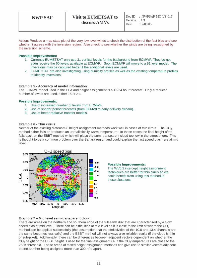
method either fails or produces an unrealistically warm temperature. In these cases the final height often falls back on the EBBT method which will place the semi-transparent cloud too low in the atmosphere. This is thought to be a common problem over the Sahara region and could explain the fast speed bias here at mid level.

Example 7 – Mid level semi-transparent cloud There are areas on the northern and southern edge of the full earth disc that are characterised by a slow speed bias at mid level. There can be difficulties at mid level as it is close to the limit of where the CO2 method can be applied successfully (the assumption that the emissivities of the 10.8 and 13.4 channels are the same becomes less valid) and the EBBT method will not always give reliable results (if the cloud is thin or sub-pixel). Additionally, there can be differences between adjacent vectors dependent on whether the CO2 height or the EBBT height is used for the final assignment i.e. if the CO2 temperatures are close to the 253K threshold. These areas of mixed height assignment methods can give rise to similar vectors adjacent to one another being assigned more than 300 hPa apart.

Possible Improvements: The WV6.2 intercept height assignment techniques are better for thin cirrus so we could benefit from using this method in these situations.

NWP SAF



12

Possible Improvements

1. Further investigation of these areas to understand better what is causing the biases. 2. Check whether the WV intercept techniques can improve height assignment at mid level 3. Are all mid level winds of dubious quality or can we flag the ones that are so that we can continue

assimilating those that are OK. Example 8 – WV 6.2 EBBT The WV6.2 EBBT heights are consistently higher than the WV7.3 EBBT and the IR10.8 EBBT for winds below about 250 hPa in height. The difference becomes more marked with increase in pressure, but is ~50 hPa at 300 hPa. A couple of factors that may influence this are errors in calibration and errors due to WV absorption above cloud top. According to Ken the 6.2 � m channel is 1K too cold and the 7.3� m channel is 1.5K too warm so there is up to 2.5K difference between 6.2 and 7.3� m channels.

White dots are for 13 April 2005, 00:30UTC, blue dots are for 13 April 2005, 10:30UTC. Collocations done on a 1x1 degree resolution grid.

NWP SAF



13

Possible Improvements

1. Recalibration at some point? (Leo to pursue?). 2. Check if there are errors allowing for WV absorption above cloud top.

Example 9 – Tracking dust We saw one example where the winds were probably produced by tracking dust. This may be quite common in the summer months over the desert region. The vectors themselves are probably fine, but the height assignment may be less good as the dust is likely to be warmer than the surrounding atmosphere and so there may be a tendency to place the vectors too low in the atmosphere. If the height assignment is not misplaced by much or if there is not very much vertical wind shear, this may not be a problem.

Met Office dust product, uses 12.0 and 10.8 channels Example 10 – Clouds modified by other processes Clouds often change shape with time. Some clouds, for example in the region of upper level tropical divergence, may be expanding outwards. The tracking will therefore represent a combination of the cloud movement and the cloud expansion. We also saw one example where the vectors at the edge of a large cloud bank were very different to those in the centre. The vectors at the edge probably provided a better guide to the movement of the whole cloud system rather than the local wind. Possible Improvements There is probably not a great deal that can be done about these situations, except possibly to get a better understanding of where and how often it happens. Example 11 – incorrect tracer location in subsequent images We saw some cases where one of the component vectors was markedly different to the others. This was probably due to the incorrect identification of the target in the search area. This could happen if there are lots of similar cloud features or if the cross-correlation requirement is quite low. Most of these cases were removed by the height assignment consistency of the component vectors requiring to be within 50 hPa (and ? other checks). On the occasions when a final vector was computed, they generally had low quality indicators and would be automatically rejected by the data assimilation systems.

Possible Improvements Investigate the likely height assignment error and typical vertical wind shear to determine if the vectors could still provide useful information on the wind field in this otherwise quite data sparse area. If it is likely to cause problems, it could be avoided by adding a dust check to the CLA. Currently the CLA will normally classify dust as low cloud. Sarah Watkin thought that a geographically restricted test to distinguish between dust and low cloud should be possible.

NWP SAF



14

Possible Improvements These cases seem to mostly look after themselves with the existing quality control at EUMETSAT. Example 12 – clear sky WV winds In the WV channel, targets are considered as clear sky if there are less than 50 cloudy pixels (~10%) in the target area. Also, low cloud is disregarded. In theory a target could contain 90% low cloud and 10% high cloud and be considered as clear sky. The low cloud should not be very prominent in the WV channels, although it probably will be visible in the WV7.3 channel at least. This low cloud or probably more often the small allowable amount of mid/high level cloud could dominate in the tracking. However, the height assignment will be based on the clear sky assignment. This could be exacerbated if there are errors in the CLA used to determine the height of the cloud for the clear/cloudy determination. The CSWV winds from EUMETSAT are still worse than the CSWV winds from NESDIS (including the unedited data). This suggests that there is room for improvement. I know Lüder had some additional concerns over the height assignment strategy, but I am not sure whether this was resolved with the December 2004 change. Possible Improvements

1. Investigate whether and how often tracking of clear sky targets is dominated by the cloud. It may not be a big problem.

2. Consider reducing the number of allowable mid/high level cloudy pixels in clear sky targets. 3. Compare methods to those used at NESDIS/CIMSS to track down what is causing the poorer

statistics for the EUMETSAT CSWV winds.

Example 13 – Very slow winds Very slow winds may not be reliable. Currently Meteosat-8 winds slower than 1m/s have their QI values reduced. This could be raised to 2.5m/s in line with Meteosat-5/6/7. Jörgen mentioned that Niels Bormann was slightly concerned by the approach of removing or reducing QI of slow winds as it leads to a fast bias in some regions. We can see this, for example, with the GOES visible winds.

The speed bias density plot shows the removal of the slow satwinds (nothing below about 3 m/s). This produces a fast bias at low wind speeds (dotted curve moves away from 1:1 line). The regions of fast bias can be seen in the map plot. They are concentrated along the west coast of America and along the ITCZ (for GOES-10 – not shown). Map plots showing wind speed confirm the fast bias is associated with background wind speeds below 5 m/s. It is possible this has little impact on the forecast model, but it may be worth considering further.

NWP SAF



15

8. Meteosat 7 / Meteosat 8 comparisons Marie and Régis had some discussions on the final afternoon and amongst other things discussed some comparisons of the Met7 and Met8 winds. Included here are some examples for the 10:30 data on the 13th April 2005. The data from Meteosat 7 and Meteosat 8 have been regridded on a 1x1 degree grid, but similar results were observed for the comparison at 0.2x0.2 degree resolution. There is no obvious speed bias and a very good correlation in the u and v components; however, there is more spread in the height assignment. A QI threshold of 80 (QI with FG check) was applied before running the comparison.

Met8 as a function of Met7 IR u wind component (m/s). 13 April 2005,10:30UTC

Met8 as a function of Met7 IR v wind component (m/s). 13 April 2005,10:30UTC

Met8 as a function of Met7 IR wind speed (m/s). 13 April 2005,10:30UTC

Met8 IR wind pressure (hPa) as a function of Met 7 IR wind pressure. 13 April 2005, 10:30UTC

Meteosat wind height assignment difference (hPa) Met8 - Met7. 13 April 2005, 10:30UTC

9. Production of AMVs from simulated imagery: (paragraph provided by Jean-Noel Thepaut) To better understand the problem of height assignment and disentangle its various sources in a more efficient way, it is proposed to go back to simulations. The idea is that NWP centres (e.g. ECMWF) provides EUMETSAT with a sequence of simulated satellite images directly generated from its model outputs. EUMETSAT ingests these images in their operational processing and provides AMVs back to the NWP centres. The advantage of this approach is that the truth is known (the NWP model) and sources of AMV height assignment errors can be more easily documented. The disadvantage is the limited resolution of the NWP model, and this perhaps explains why this idea has not been explored in more depth in the past. However, it is believed that the degree of realism of the current and near future NWP models and RT models (for example a ~20 km resolution model coupled with RTTOVcld) justifies that we go back to these

NWP SAF



16

fundamentals. Note also that the effect of a bias in radiance space on the quality of the AMVs can be easily addressed in this context. 10. NWP requirements and plans 10.1. Introduction This section provides a bit more guidance on what is most important for NWP with regards to the AMV data. We have also put together some suggestions for follow up work and listed some of the main plans for AMVs at the Met Office and ECMWF. 10.2. Current requirements • As accurate a product as possible. • Knowledge of problem areas so that they can be blacklisted or down-weighted • Vector and height errors (or if not possible at least vector and height quality indicators) attached with each

wind. • Temporal and spatial resolution less important as assimilation limited by correlated error. There are also

larger overheads storing, extracting and monitoring larger data volumes. Spatial resolution limited to one wind per 200 km/ 2 degree box at most NWP centres. Winds may be OK assimilated at 1 or 2 hour intervals in 4D-Var, but it is not clear how temporal error correlations may affect assimilation at higher temporal frequency e.g. if attempt to assimilate individual components. Until we find a way to use more information (e.g. superobbing), increased resolution (particularly spatial) is of limited use.

• Maintain good communication between producers and NWP centres and ensure that all interested parties are kept informed of any problems identified within any of the products, for example less confidence in the Met-8 WV6.2 winds due to height assignment difficulties.

10.3. Some ideas/tests • What is the geographical wind shear distribution? Height assignment error more problematic in these

areas. • What impact does an error in height assignment have on the wind assimilation? Are there some

simplified tests that could be run with some randomly introduced errors (10, 50, 100, 200 hPa). I suspect not easy.

• Can we have variable size thinning or superobbing boxes so that we use winds at greater density in regions of development or greater variability?

• Should we carry out some comparisons of AMV heights to level of best fit in our model? Systematic differences, range of values typically seen etc.

• Collocations of EUMETSAT and NESDIS winds in overlap regions. How do they compare? 10.4. Met Office plans • Continue to monitor and trial new datasets. • Produce a second analysis of the NWP SAF satellite wind monitoring report. • Develop individual observation errors for each wind. Plan to use vector and height errors/indicators

developed by wind producers. Can calculate the observation error by summing the vector error with the error in vector due to the height error. The latter will be dependent on the vertical wind shear.

• Move towards using more forecast-independent data where possible (QI2, unedited NESDIS winds). • Re-evaluate blacklisting settings and consider developing variational QC for AMVs. • Make more use of temporal information in the AMV data now we have 4D-Var. • Consider observation operator modifications to allow for AMVs representing a spatial and temporal

average. 10.5. ECMWF Plans • Continue to monitor and trial new datasets.

NWP SAF



17

• Monitor and trial the CO2 13.4/12.0 winds from EUMETSAT to check whether they are an improvement on the CO2 13.4/10.8 winds.

• Produce simulated imagery for EUMETSAT/CIMSS to produce vectors from. • Relook at Niels Bormann’s bias correction via height reassignment strategy. • Observation operator changes. 10.6. Summary of possible improvements at EUMETSAT • Work towards producing a height QI/error with each wind. • Comparison studies with CIMSS. Calculate AMVs on eachover’s imagery. • Produce AMVs from simulated imagery from ECMWF. • Improvements to height assignment including new CO2 slicing using the 12.0 channel and reintroduction

of the WV intercept techniques. • Increase in number of mid-cloud tracers by adjusting contrast thresholds and possibly altering the grid

size. • Investigations into whether a better link can be made between the pixels that dominate in the tracking and

the pixels used for height assignment. How often are there problems by just assigning the vector to the height of the coldest cloud scene?

• Improvements to the CLA. • Improvements to the identification of different cloud scenes. If this can be done accurately, there should

be improvements to the height assignment and the information could be used to identify targets with multi-level cloud, where the height assignment may be more problematic.

• Switch to using new 91 level fast delivery model output from ECMWF (including for inversion scheme). • Switch to using a standard radiative transfer model (?RTTOV). • Keep a list of problem areas for satellite winds, keep the users informed and together investigate these

areas to see whether improvements can be made. • Consider bias correcting the radiances before use. Jaime Daniels (IWW7 proceedings) showed how this

made a 50 hPa difference in the CO2 height assignment and improved the O-B statistics. • Is there a problem with the allowance for WV absorption above cloud top? • Check whether the winds produced from tracking dust are OK for use. If not include a dust check in the

CLA. • Check whether cloud presence in the clear sky targets is causing any problems. Acknowledgements We would like to thank everyone at EUMETSAT who organised and participated in the very useful discussions and meetings. This report is intended as a fairly informal record of some of the discussions that took place. We apologise for any errors or misrepresentations (memories far from perfect).

nwp saf · marie doutriaux-boucher, loa, ... (have copy of .ppt) ... an eye on met-6 winds and...

Documents