numerical shape optimization and adjoint equations - tifr...
TRANSCRIPT

Numerical shape optimization and adjoint equations
Praveen. [email protected]
Tata Institute of Fundamental ResearchCenter for Applicable Mathematics
Bangalore 560065http://math.tifrbng.res.in
TIFR-CAM18 August, 2009
Praveen. C (TIFR-CAM) Shape Optimization TIFR, 18 Aug 2009 1 / 37

Effect of shape on flow
http://www.aerospaceweb.org
Praveen. C (TIFR-CAM) Shape Optimization TIFR, 18 Aug 2009 2 / 37

Airfoils
http://www.centennialofflight.gov
Praveen. C (TIFR-CAM) Shape Optimization TIFR, 18 Aug 2009 3 / 37

Compressible flow and shocks
Mach number, M =speed of air
speed of sound
Range, R = Ma
cT
CLCD
logWi
Wf
Praveen. C (TIFR-CAM) Shape Optimization TIFR, 18 Aug 2009 4 / 37

Golf ball
http://www.aerospaceweb.org
Praveen. C (TIFR-CAM) Shape Optimization TIFR, 18 Aug 2009 5 / 37

Effect of shape on flow
http://www.aerospaceweb.org
Praveen. C (TIFR-CAM) Shape Optimization TIFR, 18 Aug 2009 6 / 37

Objectives and controls
• Objective function I(β) = I(β,Q)mathematical representation of system performance
• Control variables βI Parametric controls β ∈ Rn
I Infinite dimensional controls β : X → YI Shape β ∈ set of admissible shapes
• State variable Q: solution of an ODE or PDE
R(β,Q) = 0 =⇒ Q = Q(β)
Praveen. C (TIFR-CAM) Shape Optimization TIFR, 18 Aug 2009 7 / 37
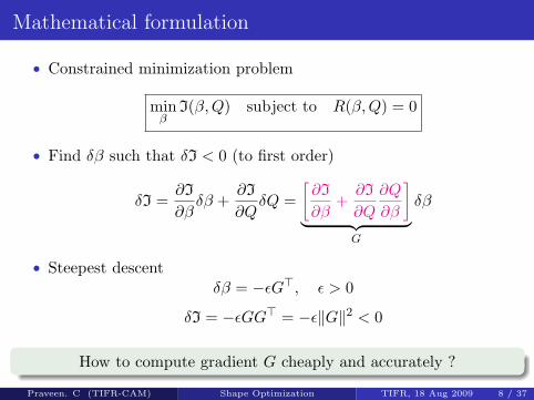
Mathematical formulation
• Constrained minimization problem
minβ
I(β,Q) subject to R(β,Q) = 0
• Find δβ such that δI < 0 (to first order)
δI =∂I
∂βδβ +
∂I
∂QδQ =
[∂I
∂β+∂I
∂Q
∂Q
∂β
]︸ ︷︷ ︸
G
δβ
• Steepest descentδβ = −εG>, ε > 0
δI = −εGG> = −ε‖G‖2 < 0
How to compute gradient G cheaply and accurately ?
Praveen. C (TIFR-CAM) Shape Optimization TIFR, 18 Aug 2009 8 / 37
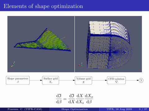
Elements of shape optimization
Shape parametersβ
Surface gridXs
Volume grid
XCFD solution
Q I
dI
dβ=
dI
dXdXdXs
dXs
dβPraveen. C (TIFR-CAM) Shape Optimization TIFR, 18 Aug 2009 9 / 37

Adjoint approach
• For shape optimization: I = I(X,Q)
dI
dX=
∂I
∂X+∂I
∂Q
∂Q
∂X
• Flow sensitivity ∂Q∂X ; costly to evaluate
• Differentiate state equation R(X,Q) = 0
∂R
∂X+∂R
∂Q
∂Q
∂X= 0
• Introducing an adjoint variable Ψ, we can write
dI
dX=
∂I
∂X+∂I
∂Q
∂Q
∂X+ Ψ>
[∂R
∂X+∂R
∂Q
∂Q
∂X
]
Praveen. C (TIFR-CAM) Shape Optimization TIFR, 18 Aug 2009 10 / 37
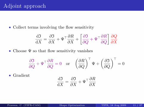
Adjoint approach
• Collect terms involving the flow sensitivity
dI
dX=
∂I
∂X+ Ψ>
∂R
∂X+[∂I
∂Q+ Ψ>
∂R
∂Q
]∂Q
∂X
• Choose Ψ so that flow sensitivity vanishes
∂I
∂Q+ Ψ>
∂R
∂Q= 0 or
(∂R
∂Q
)>Ψ +
(∂I
∂Q
)>= 0
• GradientdI
dX=
∂I
∂X+ Ψ>
∂R
∂X
Praveen. C (TIFR-CAM) Shape Optimization TIFR, 18 Aug 2009 11 / 37

Optimization steps
• β =⇒ Xs =⇒ X
• Solve the flow equations to steady-state
dQdt
+R(X,Q) = 0 =⇒ Q, I(X,Q)
• Solve adjoint equations to steady-state
dΨdt
+(∂R
∂Q
)>Ψ +
(∂I
∂Q
)>= 0 =⇒ Ψ
• Compute gradient wrt grid X
dI
dX=
∂I
∂X+ Ψ>
∂R
∂X
dI
dβ=
dI
dXdXdXs
dXs
dβ=⇒ β ←− β − εdI
dβ
Praveen. C (TIFR-CAM) Shape Optimization TIFR, 18 Aug 2009 12 / 37

Continuous and discrete approaches
• Continuous approach (differentiate and discretize)PDE −→ Adjoint PDE −→ Discrete adjoint
• Discrete approach (discretize and differentiate)PDE −→ Discrete PDE −→ Discrete adjoint
• We use the discrete approachI R(X,Q) = 0 represent the finite volume equations which are
algebraic equationsI Use ordinary calculus to differentiateI Need to compute
∂I
∂Q,
∂I
∂X,
(∂R
∂Q
)>Ψ,
(∂R
∂X
)>Ψ
Praveen. C (TIFR-CAM) Shape Optimization TIFR, 18 Aug 2009 13 / 37

Automatic differentiation
• Computer code available to compute
I(X,Q), R(X,Q)
• Code is made of composition of elementary functions
T0 = X
r′th line of program: Tr = Fr(Tr−1)Y = F (X) = Fp ◦ Fp−1 ◦ . . . ◦ F1(T0)
I Use differentiation by parts formula
Y = F ′(X)X = F ′p(Tp−1)F ′p−1(Tp−2) . . . F ′1(T0)X
I Automated using AD tools: Algorithmic Differentiation
Computer code
PAutomatic
DifferentiationNew code
P
Praveen. C (TIFR-CAM) Shape Optimization TIFR, 18 Aug 2009 14 / 37

Reverse differentiation
• Reverse mode computes transpose: (X, Y ) −→ X
X = [F ′(X)]>Y = [F ′1(T0)]>[F ′2(T1)]> . . . [F ′p(Tp−1)]>Y
• Forward sweep and then reverse sweep
Func: T0 −→ F1T1−→ F2
T2−→ . . .Tp−1−→ Fp −→ F
Grad: Tp−1, Y −→ [F ′p]T Tp−2−→ [F ′p−1]T
Tp−3−→ . . .T0−→ [F ′1]T −→ X
Forward variables Tj required in reverse order: store or recompute• Reverse mode useful to compute(
∂I
∂Q
)>,
(∂I
∂X
)>,
(∂R
∂Q
)>Ψ,
(∂R
∂X
)>Ψ
Praveen. C (TIFR-CAM) Shape Optimization TIFR, 18 Aug 2009 15 / 37

Shape parameterization
• Parameterize thedeformations[xsys
]=
[x
(0)s
y(0)s
]+[nxny
]h(ξ)
h(ξ) =m∑k=1
βkBk(ξ)
• Hicks-Henne bump functions
Bk(ξ) = sinp(πξqk), qk =log(0.5)log(ξk)
• Move points along normal toreference line AB
A B
~n
ξ
0 0.1 0.2 0.3 0.4 0.5 0.6 0.7 0.8 0.9 10
0.1
0.2
0.3
0.4
0.5
0.6
0.7
0.8
0.9
1
ξ
h(ξ)
Exact derivatives dXsdβ can be
computed
Praveen. C (TIFR-CAM) Shape Optimization TIFR, 18 Aug 2009 16 / 37

Grid deformation
• Interpolate displacement ofsurface points to interiorpoints using RBF
f(x, y) = a0 + a1x+ a2y +N∑j=1
bj |~r − ~rj |2 log |~r − ~rj |
where ~r = (x, y)
• Results in smooth grids• Exact derivatives dX
dXscan be
computed
Initial grid
Deformed grid
Praveen. C (TIFR-CAM) Shape Optimization TIFR, 18 Aug 2009 17 / 37

Test cases: airfoil shape optimization
RAE2822: M∞ = 0.729, α = 2.31o
min I =CdCd0
s.t. Cl = Cl0
Praveen. C (TIFR-CAM) Shape Optimization TIFR, 18 Aug 2009 18 / 37

RAE2822: Lift-constrained drag minimization
0 0.2 0.4 0.6 0.8 1x/c
-1
-0.5
0
0.5
1
1.5-Cp
ipoptInitial
0 0.2 0.4 0.6 0.8 1
-0.06
-0.04
-0.02
0
0.02
0.04
0.06
ipoptInitial
Praveen. C (TIFR-CAM) Shape Optimization TIFR, 18 Aug 2009 19 / 37
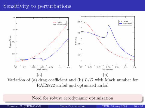
Sensitivity to perturbations
0.7 0.71 0.72 0.73 0.74 0.75 0.76Mach number
0
0.01
0.02
0.03
0.04
Dra
g co
effi
cien
t
InitialOptimized
0.7 0.71 0.72 0.73 0.74 0.75 0.76Mach number
0
50
100
150
200
Lif
t/Dra
g
InitialOptimized
(a) (b)Variation of (a) drag coefficient and (b) L/D with Mach number for
RAE2822 airfoil and optimized airfoil
Need for robust aerodynamic optimization
Praveen. C (TIFR-CAM) Shape Optimization TIFR, 18 Aug 2009 20 / 37

Wing optimization
Initial shape
Praveen. C (TIFR-CAM) Shape Optimization TIFR, 18 Aug 2009 21 / 37

Wing optimization
Optimized shape
Praveen. C (TIFR-CAM) Shape Optimization TIFR, 18 Aug 2009 22 / 37

ATR
Praveen. C (TIFR-CAM) Shape Optimization TIFR, 18 Aug 2009 23 / 37
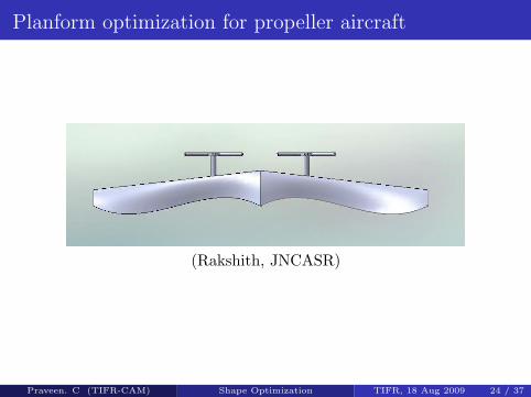
Planform optimization for propeller aircraft!"#$%&#'
'
!"#$%&'(')*+,)'-.'&/-012&'+3'4*&'+14"0"5&6',".#'6&)"#.'+74-".&6'".'4*")',+%8'3+%'-',".#',"4*'3+%'-',".#',"4*'-')4%-"#*4'2&-6".#'&6#&9'-'4-1&%'+3':;<='-.6'-'>+'2".&-%',-)*+$4;'?*&'@+.)4%-".4)'".@2$6&6'ABC':;DE9',".#'-%&-9'%++4'@*+%69'4"1'@*+%6'-.6'7+$.6)'+.'4,")4'F ;'?*&'+14"0"5&6',".#'#"G&)'
-.'".6$@&6'6%-#'%&6$@4"+.'+3'HI;>'J'-.6'-'4+4-2'6%-#'%&6$@4"+.'+3'K;E<'J;'''''
''
F-L''
''
F7L''
!"#$%&'(M'!"#$%&"'()*+$,-./$!01)*2$2-34*-564-)'#$$$!5#$*."*$,-./$!&))7-'8$(*)+$41.$4*"-&-'8$.28.#9$41.$4/-34$2-34*-564-)'$-3$+"8'-(-.2$5:$;<$4-+.3$()*$$$$$$$$$$$$$5.44.*$,-36"&-="4-)'$)($41.$4/-34>>>$
''
!"("!")*"#'
'NHO'P-0&)+.'Q9'HI(I'?'"&:3-3$)($/-'8$3&-@34*."+$(&)/$-'4.*"04-)'9'RQSQ'AT'H(>D;''NDO'U%++'V9'HIK('%*)@.&&.*A/-'8$-'4.8*"4-)'$()*$+-'-+6+$-'260.2$&)33;'P+$%.-2'+3'Q"%@%-34''''''''''''''''''D>FELM=(H'=;''N>O'W&26*$")'BBX9'D:::'?.*)2:'"+-0$)@4-+3"4-)'$)($/-'83$-'$+6&4-B.'8-'.2$4*"04)*$@*)@.&&.*$$$$$$$"**"'8.+.'439'Q"%@%-34'Y&)"#.'>'M'HDIZH<I;''N<O'P+)[;'\;'\$22+@8-%-9'D::I9'\&%)+.-2'@+00$."@-4"+.;'N=O'!"#$%&'()*+(),-.%)/0102"#1%)3%&0405"(6)C1.$D&.+.'43$)($?.*)()-&$"'2$?-*30*./$C1.)*:9'''''''''''A-07%"6#&']."G;'\%&))9'A-07%"6#&9']U9'HID(9'11;'H>EZH=='
Pressure surface
(Rakshith, JNCASR)
Praveen. C (TIFR-CAM) Shape Optimization TIFR, 18 Aug 2009 24 / 37
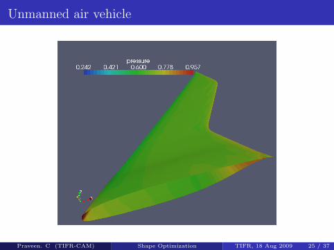
Unmanned air vehicle
Praveen. C (TIFR-CAM) Shape Optimization TIFR, 18 Aug 2009 25 / 37

Adjoint-based aposteriori error estimation
• uh = numerical solution on grid h
• Numerical analysis
‖u− uh‖ = O(hp), p > 0 as h→ 0+
How to choose the grid size ?• Functional of interest J(u)
J(u)− J(uh) = O(hp)
Choose grid so that error in J is small
Praveen. C (TIFR-CAM) Shape Optimization TIFR, 18 Aug 2009 26 / 37

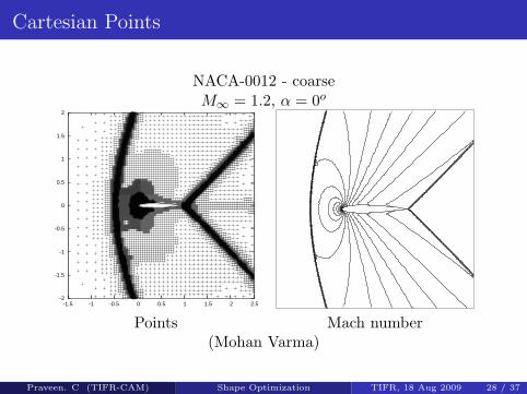
Cartesian Points
NACA-0012 - coarseM∞ = 1.2, α = 0o
-2
-1.5
-1
-0.5
0
0.5
1
1.5
2
-1.5 -1 -0.5 0 0.5 1 1.5 2 2.5
Points Mach number(Mohan Varma)
Praveen. C (TIFR-CAM) Shape Optimization TIFR, 18 Aug 2009 27 / 37
Cartesian Points
NACA-0012 - coarseM∞ = 1.2, α = 0o
-2
-1.5
-1
-0.5
0
0.5
1
1.5
2
-1.5 -1 -0.5 0 0.5 1 1.5 2 2.5
Points Mach number(Mohan Varma)
Praveen. C (TIFR-CAM) Shape Optimization TIFR, 18 Aug 2009 28 / 37

PDE with homogeneous BC
• Linear PDELu = f in D
• Adjoint operator(v, Lu) = (L∗v, u)
• Functional of interestJ = (g, u)
• Adjoint PDEL∗v = g
• Primal-dual equivalence
J = (g, u)= (L∗v, u)= (v, Lu)= (v, f)
Praveen. C (TIFR-CAM) Shape Optimization TIFR, 18 Aug 2009 29 / 37

Error estimation: homogeneous BC
fh := Luh, gh := L∗vh
The functional can be written as
J = (g, u)= (g, uh)− (gh, uh − u) + (gh − g, uh − u)= (g, uh)− (L∗vh, uh − u) + (gh − g, uh − u)= (g, uh)− (vh, L(uh − u)) + (gh − g, uh − u)= (g, uh)− (vh, fh − f) + (gh − g, uh − u)
J − Jh = −Computable error︷ ︸︸ ︷(vh, fh − f) +(gh − g︸ ︷︷ ︸
O(hp)
, uh − u︸ ︷︷ ︸O(hp)
)
J − [Jh + (vh, fh − f)] = O(h2p)
Praveen. C (TIFR-CAM) Shape Optimization TIFR, 18 Aug 2009 30 / 37
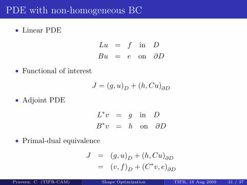
PDE with non-homogeneous BC
• Linear PDE
Lu = f in D
Bu = e on ∂D
• Functional of interest
J = (g, u)D + (h,Cu)∂D
• Adjoint PDE
L∗v = g in D
B∗v = h on ∂D
• Primal-dual equivalence
J = (g, u)D + (h,Cu)∂D= (v, f)D + (C∗v, e)∂D
Praveen. C (TIFR-CAM) Shape Optimization TIFR, 18 Aug 2009 31 / 37
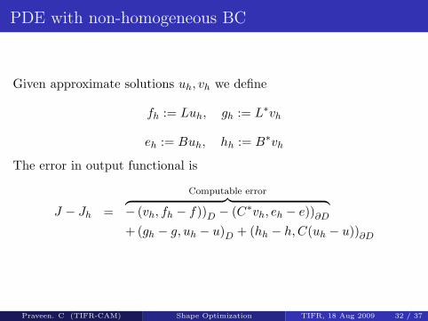
PDE with non-homogeneous BC
Given approximate solutions uh, vh we define
fh := Luh, gh := L∗vh
eh := Buh, hh := B∗vh
The error in output functional is
J − Jh =
Computable error︷ ︸︸ ︷− (vh, fh − f))D − (C∗vh, eh − e))∂D+ (gh − g, uh − u)D + (hh − h,C(uh − u))∂D
Praveen. C (TIFR-CAM) Shape Optimization TIFR, 18 Aug 2009 32 / 37

Goal-based grid adaptation
D = ∪kDk
J − Jh = −(vh, fh − f)D = −∑k
(vh, fh − f)Dk
Divide element Dk if|(vh, fh − f)Dk
| > e0
where e0 is user-specified error level.
Praveen. C (TIFR-CAM) Shape Optimization TIFR, 18 Aug 2009 33 / 37

Example: Linear scalar convection
y∂u
∂x− x∂u
∂y= 0
IsoValue-0.05263160.02631580.07894740.1315790.1842110.2368420.2894740.3421050.3947370.4473680.50.5526320.6052630.6578950.7105260.7631580.8157890.8684210.9210531.05263
Praveen. C (TIFR-CAM) Shape Optimization TIFR, 18 Aug 2009 34 / 37

Example: Linear scalar convection
y∂u
∂x− x∂u
∂y= 0
IsoValue-0.194481-0.1701-0.153846-0.137591-0.121337-0.105083-0.0888287-0.0725745-0.0563203-0.040066-0.0238118-0.007557580.008696640.02495090.04120510.05745930.07371360.08996780.1062220.146858
Error from LTMIsoValue-0.003321130.001660560.004981690.008302820.01162390.01494510.01826620.02158730.02490840.02822960.03155070.03487180.03819290.04151410.04483520.04815630.05147750.05479860.05811970.0664225
Error indicator
Praveen. C (TIFR-CAM) Shape Optimization TIFR, 18 Aug 2009 35 / 37

Application to compressible flows
• H = grid on which computations are performed• h = finer grid, perhaps h = H/2• We try to estimate
J(uh)− J(uH)
by using discrete adjoint method.
Not on that, it will tell us how to adapt the grid, in an optimalway, to control errors in J .
Praveen. C (TIFR-CAM) Shape Optimization TIFR, 18 Aug 2009 36 / 37

Application to compressible flows
0 2000 4000 6000 8000 100000.3
0.305
0.31
0.315
0.32
N
CL
JH
Jh
JhH+J
cc
(a) M∞ = 0.63, α = 2◦
0 2000 4000 6000 8000 100000.108
0.11
0.112
0.114
0.116
0.118
0.12
NC
D
JH
Jh
JhH+J
cc
(b) M∞ = 0.95, α = 0◦
Figure: Adjoint-based Lift and drag correction for NACA 0012 airfoil section
Praveen. C (TIFR-CAM) Shape Optimization TIFR, 18 Aug 2009 37 / 37