well-balanced dg scheme for euler equations with...
TRANSCRIPT

Well-balanced DG scheme forEuler equations with gravity
Praveen. [email protected]
Center for Applicable MathematicsTata Institute of Fundamental Research
Bangalore 560065
Oberseminar Mathematische StromungsmechanikInstitut fur Mathematik-der Julius-Maximilians-Universitat Wurzburg
16 April 2015
Supported by Airbus Foundation Chair at TIFR-CAM/ICTS1 / 57

Euler equations with gravity
Flow properties
ρ = density, u = velocity
p = pressure, E = total energy
Gravitational potential Φ; force per unit volume of fluid
−ρ∇Φ
System of conservation laws
∂ρ
∂t+
∂
∂x(ρu) = 0
∂
∂t(ρu) +
∂
∂x(p+ ρu2) = −ρ∂Φ
∂x∂E
∂t+
∂
∂x(E + p)u = −ρu∂Φ
∂x
2 / 57

Euler equations with gravity
Perfect gas assumption
p = (γ − 1)
[E − 1
2ρu2
], γ =
cpcv> 1
In compact notation
∂q
∂t+∂f
∂x= −
0ρρu
∂Φ
∂x
where
q =
ρρuE
, f =
ρup+ ρu2
(E + p)u
3 / 57

Hydrostatic solutions
• Fluid at rest
ue = 0
• Mass and energy equation satisfied
• Momentum equationdpedx
= −ρedΦ
dx(1)
• Need additional assumptions to solve this equation
• Assume ideal gas model
p = ρRT, R = gas constant
4 / 57

Hydrostatic solutions
• Isothermal hydrostatic state, i.e., Te(x) = Te = const, then
pe(x) exp
(Φ(x)
RTe
)= const (2)
Density
ρe(x) =pe(x)
RTe• Polytropic hydrostatic state, then we have following relations
peρ−νe = const, peT
− νν−1
e = const, ρeT− 1ν−1
e = const (3)
where ν > 1 is some constant. From (1) and (3), we obtain
νRTe(x)
ν − 1+ Φ(x) = const (4)
E.g., pressure is
pe(x) = C1 [C2 − Φ(x)]ν−1ν
5 / 57

Existing schemes
• Finite volumes
I Isothermal case: Xing and Shu [3], well-balanced WENO schemeI If ν = γ we are in isentropic case
h(x) + Φ(x) = const
has been considered by Kappeli and Mishra [1].I Desveaux et al: Relaxation schemes, general hydrostatic statesI PC and Klingenberg: isothermal and polytropic, ideal gas
• DGI Yulong Xing: ideal gas, isothermal well-balanced
6 / 57

Why well-balanced scheme
• Scheme is well-balanced if it exactly preserves hydrostatic solution.
• General evolutionary PDE
∂q
∂t= R(q)
• Stationary solution qeR(qe) = 0
• We are interested in computing small perturbations
q(x, 0) = qe(x) + εq(x, 0), ε� 1
• Perturbations are governed by linear equation
∂q
∂t= R′(qe)q
7 / 57
Why well-balanced scheme
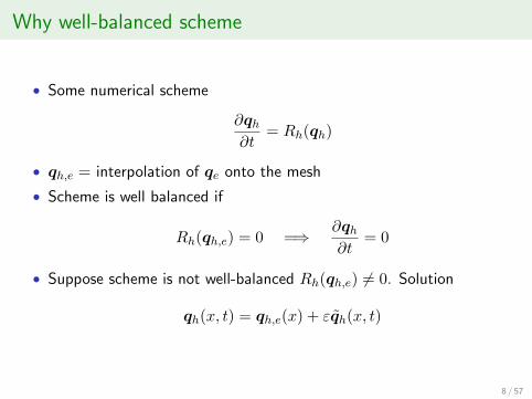
• Some numerical scheme
∂qh∂t
= Rh(qh)
• qh,e = interpolation of qe onto the mesh
• Scheme is well balanced if
Rh(qh,e) = 0 =⇒ ∂qh∂t
= 0
• Suppose scheme is not well-balanced Rh(qh,e) 6= 0. Solution
qh(x, t) = qh,e(x) + εqh(x, t)
8 / 57

Why well-balanced scheme
• Linearize the scheme around qh,e
∂
∂t(qh,e + εqh) = Rh(qh,e + εqh) = Rh(qh,e) + εR′h(qh,e)qh
or∂qh∂t
=1
εRh(qh,e) +R′h(qh,e)qh
• Scheme is consistent of order r: Rh(qh,e) = Chr‖qh,e‖
∂qh∂t
=1
εChr‖qh,e‖+R′h(qh,e)qh
• ε� 1 then first term may dominate the second term; need h� 1
• Well-balanced scheme: Rh(qh,e) = 0
∂qh∂t
= R′h(qh,e)qh
9 / 57

Scope of present work
• Nodal DG schemeI Gauss-Lobatto-Legendre nodesI Arbitrary quadrilateral cells in 2-D
• Ideal gas model: well-balanced for isothermal hydrostatic solutions
• Any consistent numerical flux
10 / 57

Finite element and well-balanced
Consider conservation law with source term
qt + f(q)x = s(q)
which has a stationary solution qe
f(qe)x = s(qe)
Weak formulation: Find q(t) ∈ V such that
d
dt(q, φ) + a(q, φ) = (s(q), φ), ∀φ ∈ V
Finite element scheme: Find qh(t) ∈ Vh such that
d
dt(qh, φh) + a(qh, φh) = (s(qh), φh), ∀φh ∈ Vh
11 / 57

Finite element and well-balanced
This is not true in general since we need to use quadratures.
FEM with quadrature: Find qh(t) ∈ Vh such that
d
dt(qh, φh)h + ah(qh, φh) = (sh(qh), φh)h, ∀φh ∈ Vh
Let
qe,h = Πh(qe), Πh : V → Vh, interpolation or projection
For the above scheme to be well-balanced, we require that
ah(qe,h, φh) = (sh(qe,h), φh)h, ∀φh ∈ Vh
because ifqh(0) = qe,h =⇒ qh(t) = qe,h ∀t
12 / 57
Mesh and basis functions
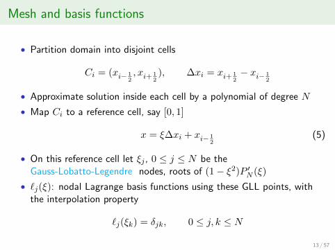
• Partition domain into disjoint cells
Ci = (xi− 12, xi+ 1
2), ∆xi = xi+ 1
2− xi− 1
2
• Approximate solution inside each cell by a polynomial of degree N
• Map Ci to a reference cell, say [0, 1]
x = ξ∆xi + xi− 12
(5)
• On this reference cell let ξj , 0 ≤ j ≤ N be theGauss-Lobatto-Legendre nodes, roots of (1− ξ2)P ′N (ξ)
• `j(ξ): nodal Lagrange basis functions using these GLL points, withthe interpolation property
`j(ξk) = δjk, 0 ≤ j, k ≤ N
13 / 57

Mesh and basis functions
• Basis functions in physical coordinates
φj(x) = `j(ξ), 0 ≤ j ≤ N
• Derivatives of the shape functions φj : apply the chain rule ofdifferentiation
d
dxφj(x) = `′j(ξ)
dξ
dx=
1
∆xi`′j(ξ)
• xj ∈ Ci denote the physical locations of the GLL points
xj = ξj∆xi + xi− 12, 0 ≤ j ≤ N
14 / 57
Discontinuous Galerkin Scheme
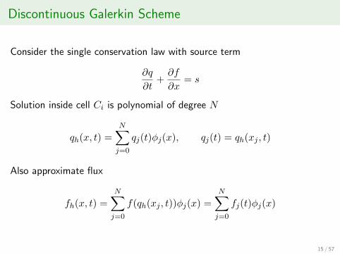
Consider the single conservation law with source term
∂q
∂t+∂f
∂x= s
Solution inside cell Ci is polynomial of degree N
qh(x, t) =
N∑j=0
qj(t)φj(x), qj(t) = qh(xj , t)
Also approximate flux
fh(x, t) =
N∑j=0
f(qh(xj , t))φj(x) =
N∑j=0
fj(t)φj(x)
15 / 57

Discontinuous Galerkin Scheme
Gauss-Lobatto-Legendre quadrature∫Ci
φ(x)ψ(x)dx ≈ (φ, ψ)h = (φ, ψ)N,Ci = ∆xi
N∑q=0
ωqφ(xq)ψ(xq)
GLL weights ωq correspond to the reference interval [0, 1].
Semi-discrete DG: For 0 ≤ j ≤ N
d
dt(qh, φj)h + (∂xfh, φj)h +[fi+ 1
2− fh(x−
i+ 12
)]φj(x−i+ 1
2
)
−[fi− 12− fh(x+
i− 12
)]φj(x+i− 1
2
) = (sh, φj)h
(6)
where fi+ 12
= f(q−i+ 1
2
, q+i+ 1
2
) is a numerical flux function.
16 / 57

Numerical flux
Numerical flux is consistent: f(q, q) = f(q)
Def: Contact property
The numerical flux f is said to satisfy contact property if for any twostates
qL = [ρL, 0, p/(γ − 1)] and qR = [ρR, 0, p/(γ − 1)]
we havef(qL, qR) = [0, p, 0]>
• states qL, qR in the above definition correspond to a stationarycontact discontinuity.
• Contact Property =⇒ numerical flux exactly support a stationarycontact discontinuity.
• Examples of such numerical flux: Roe, HLLC, etc.
17 / 57

Approximation of source term
Let
Ti = temperature corresponding to the cell average value in cell Ci
Rewrite the source term in the momentum equation as (Xing & Shu)
s = −ρ∂Φ
∂x= ρRTi exp
(Φ
RTi
)∂
∂xexp
(− Φ
RTi
)
Source term approximation: For x ∈ Ci
sh(x) = ρh(x)RTi exp
(Φ(x)
RTi
)∂
∂x
N∑j=0
exp
(−Φ(xj)
RTi
)φj(x) (7)
Source term in the energy equation
1
ρh(ρu)hsh
18 / 57

Well-balanced property
Well-balanced property
Let the initial condition to the DG scheme (6), (7) be obtained byinterpolating the isothermal hydrostatic solution corresponding to acontinuous gravitational potential Φ. Then the scheme (6), (7) preservesthe initial condition under any time integration scheme.
Proof: For continuous hydrostatic solution, by flux consistency
fi+ 12− fh(x−
i+ 12
) = 0, fi− 12− fh(x+
i− 12
) = 0
Above is true even if density is discontinuous, provided flux satisfiescontact property.
=⇒ density and energy equations are well-balanced
19 / 57

Well-balanced property
The flux fh has the form
fh(x, t) =
N∑j=0
pj(t)φj(x), pj = pressure at the GLL point xj
Isothermal initial condition, Ti = Te = const. The source term evaluated
20 / 57

Well-balanced property
at any GLL node xk is given by
sh(xk) = ρh(xk)RTe︸ ︷︷ ︸pk
exp
(Φ(xk)
RTe
) N∑j=0
exp
(−Φ(xj)
RTe
)∂
∂xφj(xk)
= pk exp
(Φ(xk)
RTe
) N∑j=0
exp
(−Φ(xj)
RTe
)∂
∂xφj(xk)
=
N∑j=0
pk exp
(Φ(xk)
RTe
)exp
(−Φ(xj)
RTe
)∂
∂xφj(xk)
=
N∑j=0
pj exp
(Φ(xj)
RTe
)exp
(−Φ(xj)
RTe
)∂
∂xφj(xk)
=
N∑j=0
pj∂
∂xφj(xk) =
∂
∂xfh(xk)
21 / 57

Well-balanced property
Since
∂xfh(xk) = sh(xk) at all the GLL nodes xk
we can conclude that
(∂xfh, φj)h = (sh, φj)h , 0 ≤ j ≤ N
and hence the scheme is well-balanced for the momentum equationalso.
22 / 57
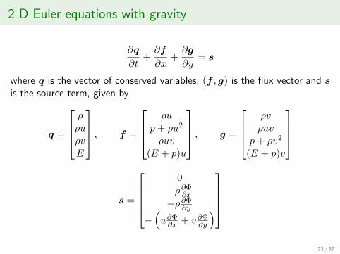
2-D Euler equations with gravity
∂q
∂t+∂f
∂x+∂g
∂y= s
where q is the vector of conserved variables, (f , g) is the flux vector and sis the source term, given by
q =
ρρuρvE
, f =
ρu
p+ ρu2
ρuv(E + p)u
, g =
ρvρuv
p+ ρv2
(E + p)v
s =
0
−ρ∂Φ∂x
−ρ∂Φ∂y
−(u∂Φ∂x + v ∂Φ
∂y
)
23 / 57

2-D hydrostatic solution
Momentum equation∇pe = −ρe∇Φ
Assuming the ideal gas equation of state
p = ρRT
and a constant temperature T = Te = const, we get
dpe = −ρedΦ = − peRTe
dΦ
Integrating this equations gives the condition
pe(x, y) exp
(Φ(x, y)
RTe
)= const (8)
We will exploit the above property of the hydrostatic state to constructthe well-balanced scheme.
24 / 57

Mesh and basis functions
A quadrilateral cell K and reference cell K = [0, 1]× [0, 1]
12
3
4
K
x
y
ξ
η
1 2
34
K
TK
1-D GLL points
ξr ∈ [0, 1], 0 ≤ r ≤ N
25 / 57
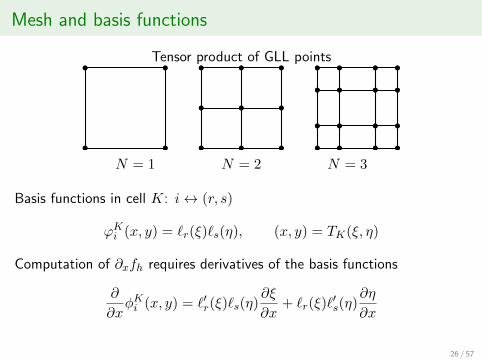
Mesh and basis functions
Tensor product of GLL points
N = 1 N = 2 N = 3
Basis functions in cell K: i↔ (r, s)
ϕKi (x, y) = `r(ξ)`s(η), (x, y) = TK(ξ, η)
Computation of ∂xfh requires derivatives of the basis functions
∂
∂xφKi (x, y) = `′r(ξ)`s(η)
∂ξ
∂x+ `r(ξ)`
′s(η)
∂η
∂x
26 / 57

DG scheme in 2-D
Consider a single conservation law with source term
∂q
∂t+∂f
∂x+∂g
∂x= s
Solution inside cell K
qh(x, y, t) =
M∑i=1
qKi (t)ϕKi (x, y), M = (N + 1)2
Approximate fluxes inside the cell by interpolation at the same GLL nodes
fh(x, y) =
M∑i=1
f(qh(xi, yi))φKi (x, y) =
M∑i=1
fiφKi (x, y)
gh(x, y) =
M∑i=1
g(qh(xi, yi))φKi (x, y) =
M∑i=1
giφKi (x, y)
27 / 57

DG scheme in 2-D
Quadrature on element K using GLL points
(φ, ψ)K =
N∑r=0
N∑s=0
φ(ξr, ξs)ψ(ξr, ξs)ωrωs|JK(ξr, ξs)|
Quadrature on the faces of the cell K
(φ, ψ)∂K =∑e∈∂K
(φ, ψ)e
where (·, ·)e are one dimensional quadrature rules using the subset of GLLnodes located on the boundary of the cell.
28 / 57

DG scheme in 2-D
Semi-discrete DG scheme: For 1 ≤ i ≤M
d
dt
(qh, φ
Ki
)K
+(∂xfh, φ
Ki
)K
+(∂ygh, φ
Ki
)K
+(Fh − F−h , φ
Ki
)∂K
=(sh, φ
Ki
) (9)
Numerical flux function
Fh = F (q−h , q+h , n), n = (nx, ny), unit outward normal to ∂K
Trace of flux on ∂K from cell K
F−h = f−h nx + g−h ny
29 / 57

Approximation of source term
Let
TK = temperature corresponding to the cell average value in cell K
Rewrite source term in the x momentum equation
s = −ρ∂Φ
∂x= ρRTK exp
(Φ
RTK
)∂
∂xexp
(− Φ
RTK
)
Approximation of source term for (x, y) ∈ K
sh(x, y) = ρh(x, y)RTK exp
(Φ(x, y)
RTK
)∂
∂x
M∑j=1
exp
(−Φ(xj , yj)
RTK
)φKj (x, y)
(10)
30 / 57

Well-balanced property
Let the initial condition to the DG scheme (9), (10) be obtained byinterpolating the isothermal hydrostatic solution corresponding to acontinuous gravitational potential Φ. Then the scheme preserves the initialcondition under any time integration scheme.
31 / 57

Limiter
• TVB limiter of Cockburn-Shu
• How to preserve hydrostatic solution ?I If residual in cell K is zero, then dont apply limiter in that cell.
32 / 57

Time integration scheme: dqdt = R(t, q)
Second order accurate SSP Runge-Kutta scheme
q(1) = qn + ∆tR(tn, qn)
q(2) =1
2qn +
1
2[q(1) + ∆tR(tn + ∆t, q(1))]
qn+1 = q(2)
Third order accurate SSP Runge-Kutta scheme
q(1) = qn + ∆tR(tn, qn)
q(2) =3
4qn +
1
4[q(1) + ∆tR(tn + ∆t, q(1))]
q(3) =1
3qn +
2
3[q(2) + ∆tR(tn + ∆t/2, q(2))]
qn+1 = q(3)
33 / 57

Numerical Results
34 / 57
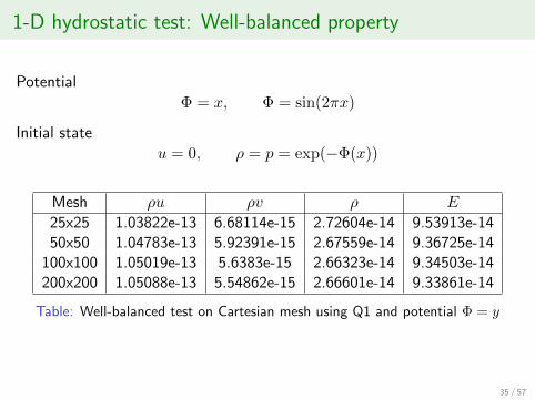
1-D hydrostatic test: Well-balanced property
Potential
Φ = x, Φ = sin(2πx)
Initial state
u = 0, ρ = p = exp(−Φ(x))
Mesh ρu ρv ρ E
25x25 1.03822e-13 6.68114e-15 2.72604e-14 9.53913e-1450x50 1.04783e-13 5.92391e-15 2.67559e-14 9.36725e-14
100x100 1.05019e-13 5.6383e-15 2.66323e-14 9.34503e-14200x200 1.05088e-13 5.54862e-15 2.66601e-14 9.33861e-14
Table: Well-balanced test on Cartesian mesh using Q1 and potential Φ = y
35 / 57

1-D hydrostatic test: Well-balanced property
Mesh ρu ρv ρ E
25x25 1.04518e-13 7.29936e-15 2.7548e-14 9.64205e-1450x50 1.04983e-13 6.03994e-15 2.69317e-14 9.43158e-14
100x100 1.05069e-13 5.68612e-15 2.69998e-14 9.39126e-14200x200 1.05089e-13 5.69125e-15 2.68828e-14 9.462e-14
Table: Well-balanced test on Cartesian mesh using Q2 and potential Φ = x
Mesh ρu ρv ρ E
25x25 9.23424e-13 1.16432e-13 2.31405e-13 8.16645e-1350x50 9.36459e-13 1.04921e-13 2.28315e-13 8.04602e-13
100x100 9.39613e-13 1.00384e-13 2.28001e-13 8.03005e-13200x200 9.40422e-13 9.89098e-14 2.2792e-13 8.02653e-13
Table: Well-balanced test on Cartesian mesh using Q1 and Φ = sin(2πx)
36 / 57
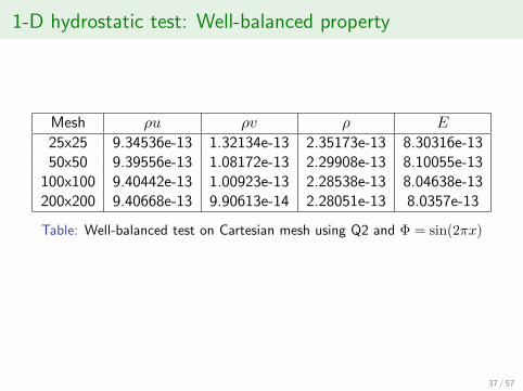
1-D hydrostatic test: Well-balanced property
Mesh ρu ρv ρ E
25x25 9.34536e-13 1.32134e-13 2.35173e-13 8.30316e-1350x50 9.39556e-13 1.08172e-13 2.29908e-13 8.10055e-13
100x100 9.40442e-13 1.00923e-13 2.28538e-13 8.04638e-13200x200 9.40668e-13 9.90613e-14 2.28051e-13 8.0357e-13
Table: Well-balanced test on Cartesian mesh using Q2 and Φ = sin(2πx)
37 / 57

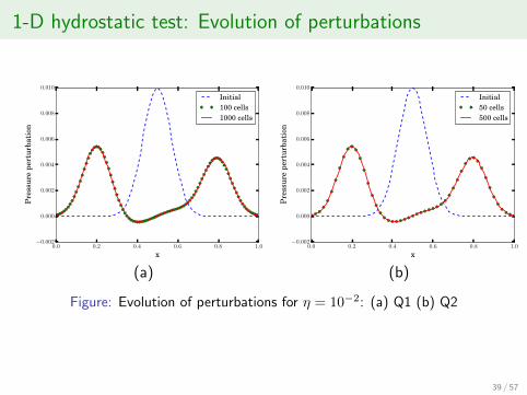
1-D hydrostatic test: Evolution of perturbations
Potential
Φ(x) = x
Initial condition
u = 0, ρ = exp(−x), p = exp(−x) + η exp(−100(x− 1/2)2)
38 / 57
1-D hydrostatic test: Evolution of perturbations
0.0 0.2 0.4 0.6 0.8 1.0
x
−0.002
0.000
0.002
0.004
0.006
0.008
0.010
Pre
ssu
rep
ert
urb
ati
on
Initial
100 cells
1000 cells
0.0 0.2 0.4 0.6 0.8 1.0
x
−0.002
0.000
0.002
0.004
0.006
0.008
0.010
Pre
ssu
rep
ert
urb
ati
on
Initial
50 cells
500 cells
(a) (b)
Figure: Evolution of perturbations for η = 10−2: (a) Q1 (b) Q2
39 / 57

1-D hydrostatic test: Evolution of perturbations
0.0 0.2 0.4 0.6 0.8 1.0
x
−0.00002
0.00000
0.00002
0.00004
0.00006
0.00008
0.00010
Pre
ssu
rep
ert
urb
ati
on
Initial
100 cells
1000 cells
0.0 0.2 0.4 0.6 0.8 1.0
x
−0.00002
0.00000
0.00002
0.00004
0.00006
0.00008
0.00010
Pre
ssu
rep
ert
urb
ati
on
Initial
50 cells
500 cells
(a) (b)
Figure: Evolution of perturbations for η = 10−4: (a) Q1 (b) Q2
40 / 57

Shock tube problem
Potential Φ(x) = x and initial condition
(ρ, u, p) =
{(1, 0, 1) x < 1
2
(0.125, 0, 0.1) x > 12
0.0 0.2 0.4 0.6 0.8 1.0
x
0.0
0.2
0.4
0.6
0.8
1.0
1.2
Den
sity
Q1, 100 cells
Q2, 100 cells
FVM, 2000 cells
0.0 0.2 0.4 0.6 0.8 1.0
x
0.0
0.2
0.4
0.6
0.8
1.0
1.2
Den
sity
Q1, 200 cells
Q2, 200 cells
FVM, 2000 cells
41 / 57

2-D hydrostatic test: Well-balanced test
PotentialΦ = x+ y
Hydrostatic solution is given by
ρ = ρ0 exp
(−ρ0g
p0(x+ y)
), p = p0 exp
(−ρ0g
p0(x+ y)
), u = v = 0
ρu ρv ρ E
Q1, 25× 25 9.85926e-14 9.85855e-14 5.32357e-14 1.55361e-13Q1, 50× 50 9.94493e-14 9.94451e-14 5.37084e-14 1.56669e-13Q1, 100× 100 9.96481e-14 9.96474e-14 5.38404e-14 1.57062e-13
Q2, 25× 25 9.9256e-14 9.92682e-14 5.39863e-14 1.57435e-13Q2, 50× 50 9.961e-14 9.96538e-14 5.41091e-14 1.57521e-13Q2, 100× 100 9.95889e-14 9.97907e-14 5.43145e-14 1.57728e-13
42 / 57

2-D hydrostatic test: Evolution of perturbation
p = p0 exp
(−ρ0g
p0(x+ y)
)+ η exp
(−100
ρ0g
p0[(x− 0.3)2 + (y − 0.3)2]
)
43 / 57

2-D hydrostatic test: Evolution of perturbation
x
y
0 0.2 0.4 0.6 0.8 10
0.2
0.4
0.6
0.8
xy
0 0.2 0.4 0.6 0.8 10
0.2
0.4
0.6
0.8
(a) (b)
Figure: Pressure perturbation on 50× 50 mesh at time t = 0.15 (a) Q1 (b) Q2.Showing 20 contours lines between −0.0002 to +0.0002
44 / 57

2-D hydrostatic test: Evolution of perturbation
x
y
0 0.2 0.4 0.6 0.8 10
0.2
0.4
0.6
0.8
xy
0 0.2 0.4 0.6 0.8 10
0.2
0.4
0.6
0.8
(a) (b)
Figure: Pressure perturbation on 200× 200 mesh at time t = 0.15 (a) Q1 (b) Q2.Showing 20 contours lines between −0.0002 to +0.0002
45 / 57
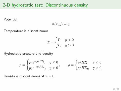
2-D hydrostatic test: Discontinuous density
Potential
Φ(x, y) = y
Temperature is discontinuous
T =
{Tl y < 0
Tu y > 0
Hydrostatic pressure and density
p =
{p0e−y/RTl , y ≤ 0
p0e−y/RTu , y > 0, ρ =
{p/RTl, y < 0
p/RTu, y > 0
Density is discontinuous at y = 0.
46 / 57
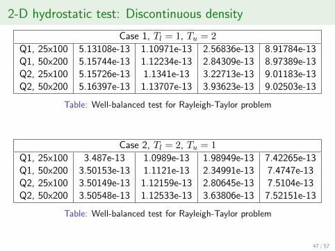
2-D hydrostatic test: Discontinuous density
Case 1, Tl = 1, Tu = 2
Q1, 25x100 5.13108e-13 1.10971e-13 2.56836e-13 8.91784e-13Q1, 50x200 5.15744e-13 1.12234e-13 2.84309e-13 8.97389e-13Q2, 25x100 5.15726e-13 1.1341e-13 3.22713e-13 9.01183e-13Q2, 50x200 5.16397e-13 1.13707e-13 3.93623e-13 9.02503e-13
Table: Well-balanced test for Rayleigh-Taylor problem
Case 2, Tl = 2, Tu = 1
Q1, 25x100 3.487e-13 1.0989e-13 1.98949e-13 7.42265e-13Q1, 50x200 3.50153e-13 1.1121e-13 2.34991e-13 7.4747e-13Q2, 25x100 3.50149e-13 1.12159e-13 2.80645e-13 7.5104e-13Q2, 50x200 3.50548e-13 1.12533e-13 3.63806e-13 7.52151e-13
Table: Well-balanced test for Rayleigh-Taylor problem
47 / 57

Order of accuracy
Exact solution of Euler equations with gravity given by
ρ = 1 + 0.2 sin(π(x+ y − t(u0 + v0))), u = u0, v = v0
p = p0 + t(u0 + v0)− x− y + 0.2 cos(π(x+ y − t(u0 + v0)))/π
Compute solution error in L2 norm at time t = 0.1
1/h ρu ρv ρ EError Rate Error Rate Error Rate Error Rate
50 0.00134154 – 0.00134154 – 0.0012837 – 0.00161287 –100 0.000335446 1.99 0.000335446 1.99 0.00032044 2.00 0.000411141 1.97200 8.35627e-05 2.00 8.35627e-05 2.00 7.97842e-05 2.00 0.00010335 1.99400 2.08348e-05 2.00 2.08348e-05 2.00 1.98754e-05 2.00 2.58109e-05 2.00
Table: Convergence of error for degree N = 1
48 / 57

Order of accuracy
1/h ρu ρv ρ EError Rate Error Rate Error Rate Error Rate
25 7.7019e-05 – 7.7019e-05 – 7.80868e-05 – 9.32865e-05 –50 9.68863e-06 2.99 9.68863e-06 2.99 9.76471e-06 2.99 1.16849e-05 2.99100 1.21506e-06 2.99 1.21506e-06 2.99 1.22031e-06 3.00 1.46256e-06 2.99200 1.52134e-07 2.99 1.52134e-07 2.99 1.52503e-07 3.00 1.8247e-07 3.00
Table: Convergence of error for degree N = 2
49 / 57

Radial Rayleigh-Taylor problem
30× 30 cells 956 cells
50 / 57
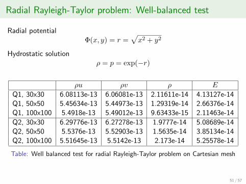
Radial Rayleigh-Taylor problem: Well-balanced test
Radial potentialΦ(x, y) = r =
√x2 + y2
Hydrostatic solutionρ = p = exp(−r)
ρu ρv ρ E
Q1, 30x30 6.08113e-13 6.06081e-13 2.11611e-14 4.13127e-14Q1, 50x50 5.45634e-13 5.44973e-13 1.29319e-14 2.66376e-14Q1, 100x100 5.4918e-13 5.49012e-13 9.63433e-15 2.11463e-14
Q2, 30x30 6.29776e-13 6.27278e-13 1.9777e-14 5.08689e-14Q2, 50x50 5.5376e-13 5.52903e-13 1.5635e-14 3.85134e-14Q2, 100x100 5.51645e-13 5.5142e-13 2.173e-14 5.25578e-14
Table: Well balanced test for radial Rayleigh-Taylor problem on Cartesian mesh
51 / 57

Radial Rayleigh-Taylor problem: Well-balanced test
ρu ρv ρ E
Q1, 956 3.03033e-16 3.23738e-16 6.66245e-16 2.11449e-16Q1, 2037 5.20653e-16 5.10865e-16 9.82565e-16 4.06402e-16Q1, 10710 2.00037e-15 1.57078e-15 2.21284e-15 4.66515e-15
Q2, 956 2.69429e-14 3.31591e-14 4.50499e-14 1.61455e-13Q2, 2037 7.68549e-14 1.1834e-13 1.01632e-13 3.84886e-13Q2, 10710 2.92633e-13 2.44323e-13 2.9449e-13 4.10069e-13
Table: Well balanced test for radial Rayleigh-Taylor problem on unstructured mesh
52 / 57
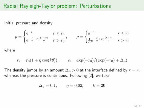
Radial Rayleigh-Taylor problem: Perturbations
Initial pressure and density
p =
{e−r r ≤ r0
e−rα
+r0(1−α)α r > r0
, ρ =
{e−r r ≤ ri1αe−
rα
+r0(1−α)α r > ri
where
ri = r0(1 + η cos(kθ)), α = exp(−r0)/(exp(−r0) + ∆ρ)
The density jumps by an amount ∆ρ > 0 at the interface defined by r = riwhereas the pressure is continuous. Following [2], we take
∆ρ = 0.1, η = 0.02, k = 20
53 / 57

Radial Rayleigh-Taylor problem: PerturbationsCartesian mesh of 240× 240 and Q1 basis
54 / 57

Summary
• Well-balanced DG scheme for Euler with gravity
• Preserves isothermal hydrostatic solutions for ideal gas model
• Any numerical flux can be used
• Cartesian, unstructured meshes
• TodoI General equation of stateI Hydrostatic solution may not be known explicitly
55 / 57

Thank You
56 / 57

References
[1] R. Kappeli and S. Mishra, Well-balanced schemes for the Eulerequations with gravitation, J. Comput. Phys., 259 (2014),pp. 199–219.
[2] Randall. J. LeVeque and Derek. S. Bale, Wave propagationmethods for conservation laws with source terms, in HyperbolicProblems: Theory, Numerics, Applications, Rolf Jeltsch and MichaelFey, eds., vol. 130 of International Series of Numerical Mathematics,Birkhauser Basel, 1999, pp. 609–618.
[3] Yulong Xing and Chi-Wang Shu, High order well-balancedWENO scheme for the gas dynamics equations under gravitationalfields, J. Sci. Comput., 54 (2013), pp. 645–662.
57 / 57