numerical modeling of three-dimensional light wood-framed buildings by
TRANSCRIPT
N U M E R I C A L M O D E L I N G OF THREE-DIMENSIONAL LIGHT WOOD-FRAMED BUILDINGS
by
M I N G H E
B . A . S c , Beijing University of Iron and Steel Technology, 1982 M . A . S c , The University of Science and Technology Beijing, 1988
M . A . Sc., The University of British Columbia, 1997
A THESIS SUBMITTED IN PARTIAL F U L F I L L M E N T OF THE REQUIREMENTS FOR THE DEGREE OF
DOCTOR OF PHILOSOPHY
iri
THE F A C U L T Y OF G R A D U A T E STUDIES THE F A C U L T Y OF FORESTRY
Department of Wood Science
We accept this thesis as conforming to the required standard
THE UNIVERSITY OF BRITISH C O L U M B I A
April 2002
© Ming He, 2002

In presenting this thesis in partial fulfilment of the requirements for an advanced
degree at the University of British Columbia, I agree that the Library shall make it
freely available for reference and study. I further agree that permission for extensive
copying of this thesis for scholarly purposes may be granted by the head of my
department or by his or her representatives. It is understood that copying or
publication of this thesis for financial gain shall not be allowed without my written
permission.
Department of _
The University of British Columbia Vancouver, Canada
Date
DE-6 (2/88)

ABSTRACT
This thesis describes the development of numerical models for predicting the
performance of three-dimensional light wood-framed buildings under static loading
conditions and subjected to dynamic excitations. The models have been implemented into a
package of nonlinear finite element programs. They satisfy the general requirements in the
study of the structural behaviour of commonly applied light-frame construction. The models
also deal with building configurations and loading conditions in a versatile manner. The
application of these programs, therefore, can provide solutions to a wide range of
investigations into the performance of wood light-frame buildings. These investigations may
include the analyses of an entire three-dimensional light-frame building, an individual
structural component, and a single connection containing one to several nails with varied
material and structural components and combined loading conditions. These buildings and
components can have irregular plan layouts, varied framing and sheathing configurations,
and different nail spacings with or without openings.
The models were verified and tested on theoretical and experimental grounds.
Theories of mechanics were applied to examine the models and related algorithms, while
experimental results were used to validate the finite element programs and to calibrate the
basic parameters required by the models. Besides the test data from previous shear wall
Abstract n

studies, three-dimensional building tests were conducted to provide the data required in the
model verification. In the experimental planning phase, the programs were intensively
employed to help select the correct configurations of the test specimens.
The experimental session contained four tests of a three-dimensional wood-framed
structure: two static tests and two earthquake tests. These tests provided extensive
information on the overall load-deformation characteristics, dynamic behaviour, torsional
deformation, influence of dead load, overturning movement, failure modes, natural
frequencies, and corresponding mode shapes of the test systems. The predicted behaviour of
the test specimens by the programs is in good agreement with test results. This indicates that
the programs are well suited for the investigation of the general behaviour of wood light-
frame systems and for the study of load sharing and torsional effects on three-dimensional
buildings due to structural and material asymmetries.
Abstract iii
T A B L E OF CONTENTS
ABSTRACT ii
LIST OF TABLES x
LIST OF FIGURES xii
NOTATION xviii
AKNOWLEDGMENT xxiv
DEDICATION xxvi
CHAPTER 1. INTRODUCTION 1
1.1. General problems 1
1.2. Objectives of the current study 3
1.3. Origin and contributions of the current study 4
1.4. Applications and future study 6
1.5. Thesis organization 7
CHAPTER 2. BACKGROUND 8
2.1. Wood light-frame buildings and their response to earthquakes 8
2.1.1. Structural roles of wood light-frame buildings 8
2.1.2. Earthquake response of wood light-frame buildings 9
Table of Contents iv
2.2. Literature review 18
2.2.1. Numerical models 18
2.2.2. Experimental studies 25
2.2.3. Studies on the system effects in building 31
2.2.4. Testing methods 35
2.2.5. Connection models 40
CHAPTER 3. THE STRUCTURAL MODEL 45
3.1. Panel element 48
3.1.1. Assumptions 48
3.1.2. Geometric and physical relationships 48
3.1.3. Shape functions 52
3.2. Frame element 59
3.2.1. Assumptions 5 9
3.2.2. Geometric and physical relationships 60
3.2.3. Shape functions 61
3.3. Connection element 62
3.3.1. Assumptions 63
3.3.2. Connection model for lateral deformations 63
3.3.3. Load-displacement relations 66
3.4. The requirements of conforming elements 69
CHAPTER 4. FORMULATION OF STATIC NONLINEAR FINITE
ELEMENT EQUATIONS 70
4.1. Principle of virtual work 70
Table of Contents v

4.2. Internal virtual work in elements
4.2.1. Internal virtual work in plate element
4.2.2. Internal virtual work in beam element
4.2.3. Internal virtual work in connection element
4.3. Formulation of external force vector
4.4. Formulation and solution of system equations
4.5. Element stress calculations
4.5.1. Panel stresses and central deflection
4.5.2. Frame bending stress
4.6. Displacement control method
4.7. Convergence considerations
4.7.1. Convergence checking and criteria
4.7.2. Ill-conditioned stiffness matrix
4.7.3. Self-adaptive procedures
4.8. Further expansion of the program
CHAPTER 5. COORDINATE TRANSFORMATION IN A THREE-
DIMENSIONAL SPACE
5.1. Coordinate transformation
5.2. Stiffness matrix transformation
CHAPTER 6. FORMULATION OF DYNAMIC NONLINEAR FINITE
ELEMENT EQUATIONS
6.1. Formulation of equations of motion
6.2. Formulation of mass matrix and vectors
Table of Contents
6.3. Formulation of damping matrix 106
6.4. Formulation and solution of system equations 109
6.5. Time-stepping procedures 110
6.6. Convergence considerations 113
6.7. Solution of eigenproblems 113
6.8. Further expansion of the program 116
CHAPTER 7. ANALYTICAL-BASED VERIFICATION OF THE FINITE
ELEMENT MODELS 118
7.1. Verification of three-dimensional transformations 119
7.2. Verification of the static finite element model 121
7.2.1. Linear cantilever beams 121
7.2.2. Beams loaded at shear center 124
7.2.3. Superposition of linear deformations 127
7.2.4. Stresses in cantilever beams 128
7.3. Verification of the dynamic finite element model 130
7.3.1. Harmonic vibration of undamped single degree of freedom system 131
7.3.2. Harmonic vibration of damped single degree of freedom system 133
7.4. Capabilities of programs 135
CHAPTER 8. PROCEDURES OF EXPERIMENTAL STUDY ON SIMPLIFIED
THREE-DIMENSIONAL BUILDINGS 139
8.1. Test facility 139
8.1.1. Capacity of shake table 140
8.1.2. Data acquisition system 140
Table of Contents vii

8.2. Determination of test buildings 142
8.2.1. Wall opening 143
8.2.2. Structural details of walls in test buildings 147
8.2.3. Structural details of roof in test buildings 151
8.2.4. The gravity load applied to test buildings 153
8.2.5. Selection of earthquake records 155
8.3. Experimental procedures 161
8.4. Brief description of two-dimensional shear wall tests 162
CHAPTER 9. EXPERIMENTAL-BASED VERIFICATION OF THE STATIC
FINITE ELEMENT MODELS 166
9.1. Experimental results of three-dimensional building under static loading
conditions 166
9.2. Prediction of behaviour of the three-dimensional buildings under static loading
conditions 169
9.3. System effects 174
9.4. Failure modes and relative movement between panel and frame 177
9.5. Prediction of the static behaviour of shear walls 181
9.6. Further expansion of the program 184
CHAPTER 10. EXPERIMENTAL-BASED VERIFICATION OF THE
DYNAMIC FINITE ELEMENT MODELS 186
10.1. Experimental results of three-dimensional building under dynamic excitation 187
10.1.1. Sine wave frequency sweep test and system fundamental natural
frequency 187
Table of Contents viii

10.1.2. Input acceleration signals 193
10.1.3. Basic parameters measured during the tests 196
10.2. Prediction of the dynamic behaviour of three-dimensional buildings 204
10.2.1. Natural frequencies and mode shapes 204
10.2.2. Comparison of predicted building behaviour and results from Test Three 206
10.3. Failure modes 210
10.4. Predictions of the dynamic behaviour of shear walls 215
10.5. Further expansion of the program 219
CHAPTER 11. CONCLUSIONS 221
BIBLIOGRAPHY 226
APPENDIX A. PROGRAM USER'S MANUAL 234
A. 1. Introduction 234
A.2. Modeling 234
A.3. Input and output files 236
A.4. Structures and control parameters of input files 238
A.4.1. Input file one - Titles 238
A.4.2. Input file two - Input data 239
A.4.3. Input file three - Cyclic protocol 257
A.4.4. Input file four - Time-acceleration history 258
A.4.5. Examples of input files 259
A.4.6. Examples of the output file of an eigensystem 266
A.5. Viewing graphic files generated by the postprocessor 267
Table of Contents ix
LIST OF TABLES
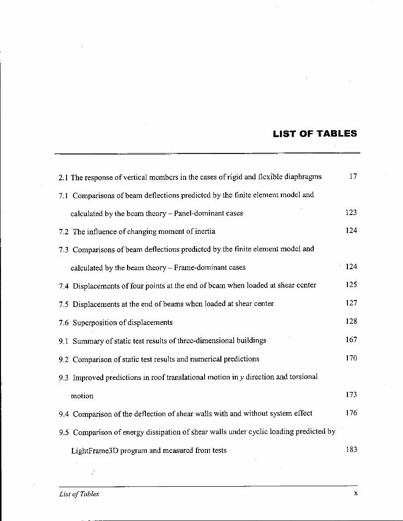
2.1 The response of vertical members in the cases of rigid and flexible diaphragms 17
7.1 Comparisons of beam deflections predicted by the finite element model and
calculated by the beam theory - Panel-dominant cases 123
7.2 The influence of changing moment of inertia 124
7.3 Comparisons of beam deflections predicted by the finite element model and
calculated by the beam theory - Frame-dominant cases 124
7.4 Displacements of four points at the end of beam when loaded at shear center 125
7.5 Displacements at the end of beams when loaded at shear center 127
7.6 Superposition of displacements 128
9.1 Summary of static test results of three-dimensional buildings 167
9.2 Comparison of static test results and numerical predictions 170
9.3 Improved predictions in roof translational motion in y direction and torsional
motion 173
9.4 Comparison of the deflection of shear walls with and without system effect 176
9.5 Comparison of energy dissipation of shear walls under cyclic loading predicted by
LightFrame3D program and measured from tests 183
List of Tables x
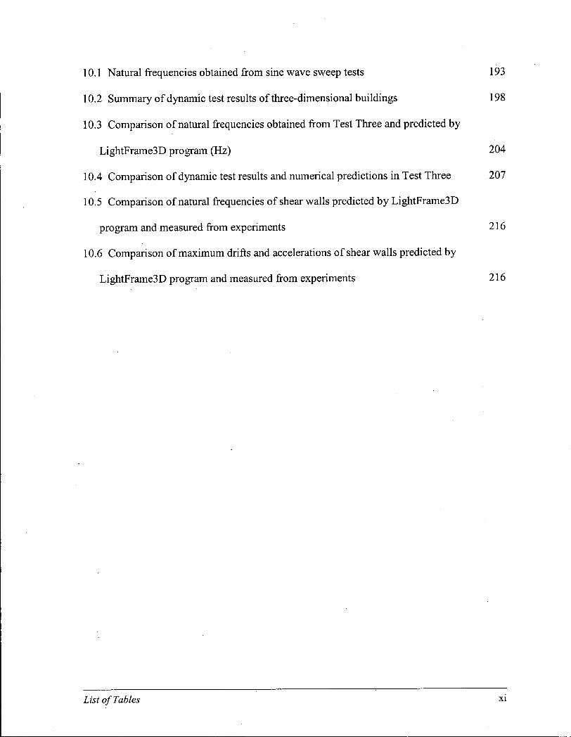
10.1 Natural frequencies obtained from sine wave sweep tests 193
10.2 Summary of dynamic test results of three-dimensional buildings 198
10.3 Comparison of natural frequencies obtained from Test Three and predicted by
LightFrame3D program (Hz) 204
10.4 Comparison of dynamic test results and numerical predictions in Test Three 207
10.5 Comparison of natural frequencies of shear walls predicted by LightFrame3D
program and measured from experiments 216
10.6 Comparison of maximum drifts and accelerations of shear walls predicted by
LighfFrame3D program and measured from experiments 216
List of Tables xi

LIST OF FIGURES
2.1 Load distribution in vertical members when diaphragm is rigid 14
2.2 Load distribution in vertical members when diaphragm is flexible 17
2.3 Seismic response of a building modeled by Chehab (1982) 19
2.4 Global degrees of freedom for house model by Gupta and Kuo (1987) 20
2.5 A three-dimensional finite element model built by Kasai et al. (1994) 21
2.6 Two-storey building test in the CUREE-Caltech wood-frame project (Folz et al. 28
2001)
2.7 Shake table tests of Earthquake 99 project 30
2.8 Three-dimensional view of test structure (Phillips 1993) 33
2.9 L-shaped test house (Foliente et al. 2000) 35
2.10 General load-displacement relationship of a wood structure 36
2.11 General hysteresis loops of a wood structure with a monotonic push-over curve 37
2.12 Nail load-displacement model (Foschi 1974, 1977) 41
2.13 Modeled hysteresis loops of nailed wood joints by various researchers 42
3.1 Basic element unit 47
3.2 Nodal and element degrees of freedom 47
List of Figures xii

3.3 Middle plane extension of plate element
3.4 Derivation of shear strain components
3.5 Natural coordinate system
3.6 Twist deformation of a horizontal beam element
3.7 Connection finite element model for lateral load
3.8 Nail connector stress-strain relationship
3.9 Connection lateral deformations
3.10 Connection load-displacement relationships
4.1 General three-dimension body
4.2 Uniformly distributed load acting on an element
4.3 Newton-Raphson iteration starting from point a and converging at point b
4.4 Cyclical searching in the Newton-Raphson iteration method
5.1 Coordinate transformation
5.2 Mapping of stiffness coefficients in element stiffness matrix (only exterior panel
considered)
6.1 Rayleigh damping
6.2 Mass-proportional damping and stiffness-proportional damping
7.1 Test cases used in verifications
7.2 Test cantilever beams with varied cross-section profiles
7.3 Channel sections were loaded at shear center or at corner 1
7.4 Output graphics from program showing the deformations at the end of beams
7.5 Cantilevered angle sections were loaded at shear center
7.6 Output graphics from program showing the deformations at the end of beams
List of Figures
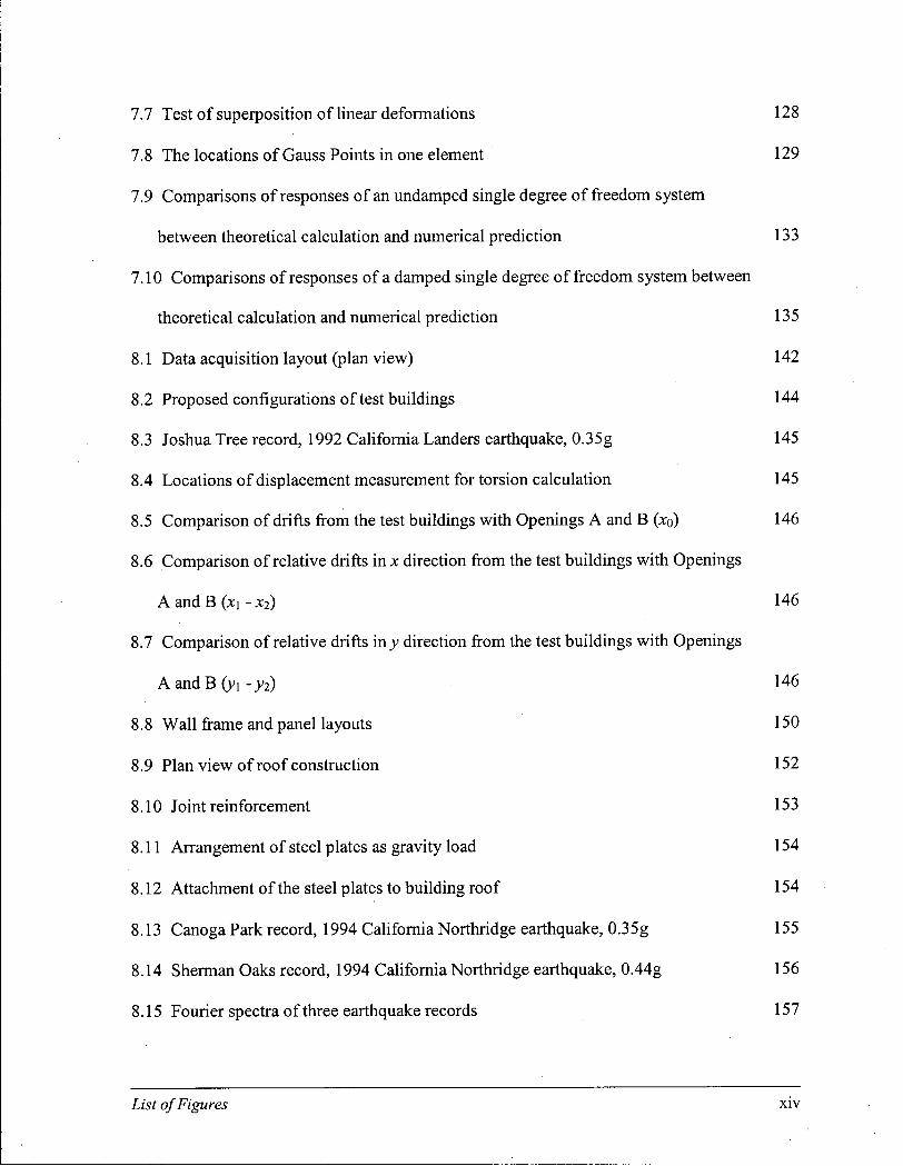
7.7 Test of superposition of linear deformations 128
7.8 The locations of Gauss Points in one element 129
7.9 Comparisons of responses of an undamped single degree of freedom system
between theoretical calculation and numerical prediction 133
7.10 Comparisons of responses of a damped single degree of freedom system between
theoretical calculation and numerical prediction 135
8.1 Data acquisition layout (plan view) 142
8.2 Proposed configurations of test buildings 144
8.3 Joshua Tree record, 1992 California Landers earthquake, 0.35g 145
8.4 Locations of displacement measurement for torsion calculation 145
8.5 Comparison of drifts from the test buildings with Openings A and B (xo) 146
8.6 Comparison of relative drifts in x direction from the test buildings with Openings
A and B (xi - x 2) 146
8.7 Comparison of relative drifts my direction from the test buildings with Openings
A and B (yi - y2) 146
8.8 Wall frame and panel layouts 150
8.9 Plan view of roof construction 152
8.10 Joint reinforcement 153
8.11 Arrangement of steel plates as gravity load 154
8.12 Attachment of the steel plates to building roof 154
8.13 Canoga Park record, 1994 California Northridge earthquake, 0.35g 155
8.14 Sherman Oaks record, 1994 California Northridge earthquake, 0.44g 156
8.15 Fourier spectra of three earthquake records 157
List of Figures xiv
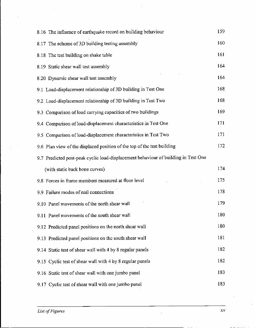
8.16 The influence of earthquake record on building behaviour 159
8.17 The scheme of 3D building testing assembly 160
8.18 The test building on shake table 161
8.19 Static shear wall test assembly 164
8.20 Dynamic shear wall test assembly 164
9.1 Load-displacement relationship of 3D building in Test One 168
9.2 Load-displacement relationship of 3D building in Test Two 168
9.3 Comparison of load carrying capacities of two buildings 169
9.4 Comparison of load-displacement characteristics in Test One 171
9.5 Comparison of load-displacement characteristics in Test Two 171
9.6 Plan view of the displaced position of the top of the test building 172
9.7 Predicted post-peak cyclic load-displacement behaviour of building in Test One
(with static back bone curves) 174
9.8 Forces in frame members measured at floor level 175
9.9 Failure modes of nail connections 178
9.10 Panel movements of the north shear wall 179
9.11 Panel movements of the south shear wall 180
9.12 Predicted panel positions on the north shear wall 180
9.13 Predicted panel positions on the south shear wall 181
9.14 Static test of shear wall with 4 by 8 regular panels 182
9.15 Cyclic test of shear wall with 4 by 8 regular panels 182
9.16 Static test of shear wall with one jumbo panel 183
9.17 Cyclic test of shear wall with one jumbo panel 183
List of Figures xv
9.18 Predicted post-peak cyclic load-displacement relationship of shear wall 184
10.1 Amplitudes in the primary direction in the first frequency range 190
10.2 Amplitudes in two directions in the first frequency range 190
10.3 Comparison of the phases of two signals in the first frequency range 190
10.4 Amplitudes in the secondary direction in the second frequency range 191
10.5 Amplitudes in two directions in the second frequency range 191
10.6 Comparison of the phases of two signals in the second frequency range 191
10.7 Phases of two signals in the primary direction in the third frequency range 192
10.8 Phases of two signals in the secondary direction in the third frequency range 192
10.9 Three natural frequencies of building in Test Three 193
10.10 Three natural frequencies of building in Test Four 193
10.11 Comparison of the 5% damped acceleration response spectra 195
10.12 Input earthquake record (Joshua Tree, east-west, 0.35 g) used in Test Three 196
10.13 Input earthquake record used in Test Four 196
10.14 Response-time history of Test Three 201
10.15 Response-time history of Test Four in the primary direction 202
10.16 Response-time history of Test Four in the secondary direction 203
10.17 Predicted three mode shapes 205
10.18 Comparison of drift and acceleration in Test Three 207
10.19 Comparison of acceleration frequency range 208
10.20 Comparisons of drifts of four walls in Test Three 210
10.21 Nail withdrawal and pulling through failure modes 211
10.22 Insignificant permanent deformation in end wall 212
List of Figures xvi

10.23 Comparison of drifts of four walls in Test Four 213
10.24 Damages in the east end wall 214
10.25 Two nails in fracture modes 214
10.26 Dynamic responses of shear wall with 4 by 8 regular panels 217
10.27 Dynamic responses of shear wall with one jumbo panel 217
10.28 Comparison of Fourier spectra of shear walls predicted by LightFrame3D
program and from tests
List of Figures xvii

NOTATION
A = area.
a = degree of freedom vector, function of time,
a = relative mass acceleration vector.
ag = ground acceleration vector.
a, = absolute acceleration vector.
C = viscous damping coefficient.
c = element damping matrix.
D = dead load applied to test building, kN.
dA = differential surface area of an infinitesimal element.
dV - differential volume of an infinitesimal element.
E = total energy dissipation of test building, Nm.
Ex, Ey - Young's moduli.
F i = inertia forces.
F = resultant reaction force.
F m a x = maximum resultant reaction force.
fs = resistant force vector, depending on deformation histories.
Notation xviii

f = force containing the contributions from the linear and nonlinear
behaviour of panel and frame members and from the nonlinear behaviour of nail connections.
/ = natural frequency.
Gxy = shear modulus.
H - height of frame or beam.
I = unit matrix.
/ = moment of inertia.
i , j , k = unit vectors.
J = Jacobian matrix.
K = generalized stiffness matrix.
KT = global tangent stiffness matrix.
(K)i = linear part of global tangent stiffness matrix.
(K)N = nonlinear part of global tangent stiffness matrix.
K - initial stiffness; system stiffness.
kr = element tangent stiffness matrix.
(k)z. = linear part of element tangent stiffness matrix.
(k)N = nonlinear part of element tangent stiffness matrix.
L - length of beam.
/,, mi, - direction cosines, / = 1, 2, 3.
M / = generalized mass matrix.
M = system mass.
m = element mass matrix.
mu, mw = mass vectors related to ground acceleration components.
Notation xix
Na, Lot, Moi = shape functions.
N 0 , L 0 , M 0 = shape functions, function of space.
N = number of integration points.
Oc\, ci, a, C4 = uplift displacements measured at four corners of building, mm.
P = force.
P m a x = maximum load carrying capacity of test building (static) or maximum
effective earthquake force applied to test building (dynamic), kN.
Qx, Qy, Q z = shape function combinations.
Q = first moment of area.
Qo = intercept of the asymptote.
Q\ = asymptotic stiffness.
R = external load vector.
Rs = body force vector.
Rc = external concentrated force vector.
Rs = external surface force vector.
Rx, Ry, Rz = projections of a force in x, y, and z directions.
rB, rs = body forces and surface forces, respectively.
r = ratio of moment inertia.
T = transformation matrix.
t = thickness of panel; time.
u = arbitrary displacement field.
u, v, w = displacement fields in x, y and z directions, respectively, functions of
space and time.
Notation xx

ii, v, w = nodal acceleration vectors in x, y and z directions, respectively.
i i g , w g = ground acceleration components in x (horizontal) and z directions,
respectively.
ii,, w, = absolute nodal acceleration vectors in x and z directions, respectively.
us, vs, ws = the small displacements of a point in the middle plane of the plate
element during deformation in the x, y and z directions, respectively.
u, v = the small displacements caused by axial deformation only in the x and
y directions, respectively.
iig0 = acceleration amplitude of harmonic excitation.
V = volume.
Wi, Wj = weighting factors.
Xj, Yi, Zi = global nodal coordinate system.
Xi,Yi,Zi = local nodal coordinate system.
X°, Y°, Z° = identity vectors along the edges of the element in X, Y , and Z
directions, respectively.
x,y,z = Cartesian coordinate system.
xc, yc = central coordinates of plate element.
a, P = damping coefficients.
Ax, Ay = side lengths of plate element.
A = displacement or drift.
A m a x = displacement at Fmax.
Notation xxi
A* = ultimate displacement of test building in x direction at the maximum
load Pmax in static tests; maximum displacement of test building in x direction in dynamic
tests, mm.
Ay = maximum displacement of test building in y direction in both static
and dynamic tests, mm.
8a = virtual displacement vector.
8Wi, 5Wg = internal virtual work and external virtual work, respectively.
8Wx, 5Wy, 8WZ= virtual work done by a force inx, y, and z directions.
du, 8v, Sw = components of a virtual displacement in x, y, and z directions.
5e = virtual strain vector.
jxy = shear strain.
4, n = variables of natural coordinate system.
4', r\' = natural coordinates for loading patch.
8 = normal strain vector.
Srf, S/r = tolerances.
£* , Ey, sz
= the components of normal strain in x, y, and z directions.
£x,e'y = the components of normal strain due to stretch,
s", e" = the components of normal strain due to bending.
C, = damping ratio.
0 = maximum torsional rotation of the roof of test building about the
vertical axis, which passes through the center of mass of the roof diaphragm, rad.
A = ap xp diagonal matrix listing the corresponding eigenvalues.
Notation xxii

X - eigenvalue,
v^y, vyx = Poisson's ratios.
CT = normal stress vector.
<jx, Gy, CTZ = the components of normal stress in x, y, and z directions,
ay = yield stress of steel connector,
x = time instance.
<D = an n x p matrix with its columns equal to the p eigenvectors and its
rows equal to the n system degrees of freedom.
<|> = eigenvector.
— global out-of-balance load vector.
vj/e = element out-of-balance load vector,
co = circular natural frequency of a structural system.
a>o = circular forcing frequency of harmonic excitation.
Notation xxiii

ACKNOWLEDGMENT
In every stage of fulfilling the tasks associated with the completion of this thesis, I am
grateful to the professors, technicians and colleagues who have helped me in many ways.
First, I sincerely thank Dr. F. Lam for the guidance and the financial support that he
has given to me during the whole program. His precious advice and opinion have greatly
shaped my view of timber structural engineering and my research on the modeling of wood
building systems.
I also express my gratitude to Prof. R. Foschi, with whom I have made many fruitful
discussions on the subjects related to the research project. His invaluable theoretical
instructions and suggestions were very critical and helpful iri the problem solving and in the
finite element programming and have influenced the whole structure of the current study.
M y heartfelt appreciation also goes to Dr. H. Prion. His knowledgeable and
informative ideas about wood structural design led our experiments to success. He has
always been very generous to me with time, advice and instruction in both theoretical and
experimental work over the years.
Whenever I used the fundamental concepts of the structural dynamics as an important
tool in my whole Ph.D. study, I could not forget the expert instruction and assistance given
by Dr. C. Ventura. I certainly want to give my sincere thanks to him.
Acknowledgment xxiv

During the entire experiment session, it has been my privilege to work with the
laboratory technicians, who provided continuous assistance in every detailed piece of work.
Special thanks are given to H . Nichol, the technician in the Earthquake Engineering
Laboratory of the Department of Civi l Engineering, for his significant technical contributions
to the experimental studies. Further thanks are given to D. Hudniuk and H. Schrempp,
technicians in the Department of Civi l Engineering, for their technical support.
Moreover, I gratefully acknowledge the comments and suggestions given by my
colleagues F. Yao and Y . T. Wang. The discussions with them regarding finite element
programming were always beneficial. J. Durham is thanked for providing the experimental
data from her study.
Finally, the Department of Civi l Engineering and the Department of Wood Science
are thanked for their support with equipment, materials and finances.
Acknowledgment xxv

To my wife, Yingmei
and my son, Da
Dedication xxvi
CHAPTER 1
INTRODUCTION
1.1. General problems
Low-rise residential houses and small commercial buildings in North America are
conventionally light-frame structures using wood-based materials. Typically, they are
composed of two-dimensional diaphragm systems (e.g. shear walls, floors, ceilings, and
roofs) and are highly indeterminate. These wooden structural systems are generally believed
to perform well under wind and seismic loading when carefully constructed. This
performance could be attributed to the high strength-to-weight ratio of timber as a building
material, the redundancy of the whole system, and the ductility of the connections.
However, as has been shown in past earthquakes and hurricanes, the structural
integrity of wood frame buildings under the action of natural hazards is not necessarily
guaranteed, especially in multi-storey buildings with asymmetrical geometry. For many
years, a large amount of experimental and analytical work has been done to understand the
structural behaviour of wood based light-frame systems. The work, to a great extent, has
been limited to the study of two-dimensional structural components, such as shear walls, roof
and floor diaphragms, and metal connectors and fasteners, under static monotonic or cyclic
loading. Experiments on full-scale light-frame houses have seldom been done due to high
test costs and demands. The knowledge obtained so far about the structural behaviour of
Chapter 1 Introduction 1

complete wood buildings is mainly derived from construction practice and a few
experimental studies on major structural components.
Analytical methods were also developed by a few researchers to predict the structural
performance of an entire building. The numerical studies on the light-frame structures
mentioned above reveal that further studies on some important issues still need to be
performed. These issues include (1) at component level, the influence of nail type, spacing
and pattern, panel discontinuity and reinforcement, wall aspect ratio, and new construction
techniques; and (2) at structural level, the influence of dead load and inertia mass, ground
acceleration excitation, load sharing among components, and load path in the structure.
A literature review also shows that in the early stages of analytical studies of wood
buildings, the three-dimensional timber structures were modeled either by simplified closed-
form equations (such as Yasumura et al. 1988, Schmidt and Moody 1989) or by linear finite
elements under mainly static lateral loads. In recent years, progress has been made in the
simulation of three-dimensional wood light-frame buildings. The complications of both
actual structural behaviour and programming algorithm make it difficult to develop a model
for nonlinear dynamic analysis with refined finite elements. With the development of
analytical techniques and computational tools, and with increasing knowledge of wood
structural behaviour, it is of great interest and need to develop rational models to analytically
predict the structural performance of three-dimensional buildings by means of the nonlinear
finite element method. In the investigation of the performance of light-frame construction,
reliable numerical models possess obvious cost advantages over experimental methods, even
though the latter cannot be completely replaced. Analytical approaches can dramatically
reduce time and cost in experiments. Also, they are applicable to cases that are not feasible
Chapter 1 Introduction 2

in an experimental study. For example, in a parametric study or in development of a
response surface, a large number of cases with different parameter combinations should be
considered. While a numerical model can easily fulfill the task by altering relevant
parameters, it is very difficult to do so within a short time by experimental methods.
1.2. Objectives of the current study
Based on the literature survey and the research needs, a study was initiated, the
overall objective being to develop robust and reliable numerical models capable of predicting
the response of three-dimensional wood light-frame buildings subjected to static loading
and/or dynamic earthquake excitation. The models should also be applicable to the structural
components and individual connections. The following procedures are followed to achieve
this objective:
(1) Development of a nonlinear finite element program for panelized structures that
are in three-dimensional space and are under static monotonic loading;
(2) Development of a nonlinear finite element program with mechanics based nail
model, capable of analyzing structures under static cyclic loading;
(3) Development of a finite element program to calculate a number of the lowest
eigenvalues (natural frequencies) and corresponding eigenvectors (mode shapes) of the
structure under investigation;
(4) Development of a nonlinear finite element program for a full analysis of structures
under dynamic earthquake excitation;
(5) Verification of numerical models by means of mechanics theories and
experimental results from previous shear wall tests and newly conducted three-dimensional
shaking table tests on a model building; and
Chapter 1 Introduction 3
(6) Application of the programs with experimental input to study load path, load
sharing, and torsion effect, which are significant in a three-dimensional structural assembly.
1.3. Origin and contributions of the current study
The development of three-dimensional structural analysis models is based on a
diaphragm analysis program (PANEL) written by Foschi (1997). This program was selected
as a starting point because its structure possesses many features that are deemed necessary in
a three-dimensional numerical simulation, even though it is only applicable to two-
dimensional light-frame components under static monotonic loading. In the new model
development, the following theoretical contributions are believed to be important and critical:
(1) Introduction of coordinate transformations into finite element models so that the
behaviour of three-dimensional structures can be described. In the process of transformation
of local element stiffness matrices into a global stiffness matrix, the "substructuring"
technique is adopted. Under this technique, panel elements and frame elements, which are
under different coordinate systems, can be assembled into one global system without
increasing the complexity of the analysis.
(2) Introduction of a general mechanics-based nail connection model, HYST (Foschi
2000) into the newly developed finite element models. This makes the models capable of
performing the cyclic and dynamic analyses by calculating the hysteresis loops in mechanical
connections from basic material properties, thus enabling them to adapt automatically to any
input history, with respect to either force or displacement. This model considers a nail
connector as elasto-plastic beam acting on wood, a nonlinear medium that only acts in
compression. It permits gaps to be formed between the connector and the surrounding
medium. The model can then develop pinching as gaps are formed, and the energy
Chapter 1 Introduction 4

dissipation in a connection's deformation history can therefore be accurately represented.
During calculation, only basic material properties of the connector and the embedment
characteristics of the wood medium are required. These characteristics make the HYST
model a distinct one from other empirical curve-fitting models.
(3) Modeling of deformations and displacements of nail connection elements between
sheathing panels and frame members in three directions at each nail location. The lateral
deformations of nail connection are modeled by a spring element in each of the x and y
direction in the panel plane. The nail withdrawal or the panel-frame contact is modeled in a
direction perpendicular to the panel plane (z direction).
(4) Contribution of load control and displacement control as two options in
simulations. In static and cyclic analyses, sometimes, the displacement control method is
more desirable. It allows the analysis to go beyond the system's maximum capacity to
provide a complete load-displacement path. Also, it can easily follow the multiple load-
unloading-reloading path to present stiffness and strength degradations and pinching effects.
This is difficult in the load control method because of numerical stability problems.
(5) Introduction of the cyclic analysis procedure into the finite element models. Most
of previously developed numerical programs could not perform cyclic calculation due to both
the connection models and the load control mode that these programs used. The cyclic test is
an important step in the study of woodframe structures to understand the energy dissipation
mechanism and the hysteresis behaviour in a wood structure. The capability of performing a
cyclic analysis allows the models to carry out all three major structural analysis procedures
and therefore fills the gap between the static analysis and dynamic analysis.
This study is unique and original because it is the first attempt to
Chapter 1 Introduction 5
(1) predict the behaviour of an entire building, instead of individual components,
under static monotonic loading, cyclic loading, and dynamic earthquake excitation,, by
building three-dimensional refined finite element models;
(2) implement a mechanics-based connection model that makes the analysis more
general;
(3) integrate numerical modeling and experimental study into one project, therefore
providing instant opportunities to verify the models and to predict the building behaviour;
(4) verify the models extensively by mechanics theories and by using a database from
both past building components and present three-dimensional building tests; and
(5) build a database that contains research results from analytical and experimental
studies and that can benefit future studies in wood-based light-frame structures and
performance-based design in wood construction practice.
1.4. Applications and future study
The programs (LightFrame3D) are designed to evaluate and predict the structural
response of a three-dimensional light-frame building with varied material, structural, and
loading combinations. Load control or displacement control can be used as input history in
the static analysis. The structures can be loaded either monotonically or cyclically. They
can also be excited by dynamic ground acceleration with constant concentrated or distributed
loads being applied simultaneously. A post-processor of the model provides information on
the deformation, strength, and failure mode of the structural components.
As an analytical tool in future studies, the programs possess the capacity to perform
extensive parametric studies and system identification. A well-understood structural
behaviour and a carefully-defined load distribution in a building would provide useful
Chapter 1 Introduction 6

guidelines in light-frame building design. The programs, as a benchmark, can be further
improved and expanded. It is generally believed that the numerical evaluation of the
dynamic response of a nonlinear wood light-frame system with numerous degrees of freedom
is computationally demanding. However, with the rapid development of computer
technology, this shortcoming will be alleviated. For the time being, to make these programs
run more efficiently, new solution techniques have to be introduced. Interfaces between the
current finite element programs and commercial software are also needed to enhance the
user-friendliness of the pre-processor and post-processors. Furthermore, new functions can
be added to the programs to satisfy broader requirements in the research and study of light
wood frame systems.
1.5. Thesis organization
This thesis describes all the procedures in developing nonlinear finite element models
for three-dimensional light wood frame building systems.
This thesis first presents a survey of previous research work on light-frame building
systems with both analytical and experimental methods. Based on this survey, the most
important research needs of the current study are identified. The thesis describes in detail the
structures of numerical models and the formulations of finite element equations for both
static and dynamic situations, followed by the model verifications by mechanics theories.
The capacity of the programs and their potential applications are also addressed. The
limitations in the study are discussed at the end of appropriate chapters. The experiments, as
an integral component of the study in providing a database in model verification, are also
presented in detail. Lastly, the comparison between predictions made by the programs and
actual results from tests is presented.
Chapter 1 Introduction 7

CHAPTER 2
BACKGROUND
2.1. Wood light-frame buildings and their response to earthquakes
2.1.1. Structural roles of wood light-frame buildings
In North America, wood light-frame construction is primarily used for single-family
housing, low- to mid-rise multi-family residential buildings, and low-rise commercial
structures. These buildings usually consist of a few typical structural components, such as
vertical diaphragms (shear walls) and horizontal diaphragms (floors and roofs). These
components play critical roles in resisting various loads, including those induced by
earthquake ground motion, to retain the structural integrity of the whole system.
Shear walls are the major lateral load-carrying components in a wood frame system.
The structural details of shear walls, including framing and sheathing layout and nail spacing,
have a significant impact on the overall performance of building system (He 1997). Shear
walls need to resist the in-plane lateral loads caused by wind and ground motion during an
earthquake. These lateral loads can be either the forces directly added on shear walls or the
forces transferred from floor and roof diaphragms. Shear walls are also required to carry out-
of-plane loads, vertical dead loads, live loads, and vertical components of wind and seismic
loads. Roof and floor diaphragms mainly need to withstand dead loads and live loads from
building materials, occupants, or rain and snow, to carry transverse and lateral loads
Chapter 2 Background.

generated by wind or during earthquakes, and to transfer those loads through the vertical
lateral load resisting systems to the foundation.
A well-constructed moderately sized wood light-frame building is a very efficient and
ductile system. It has a history of good performance under seismic loading conditions. This
could be attributed to the following characteristics:
(1) a high strength-to-weight ratio of wood material;
(2) redundancy of the system due to a large number of closely spaced members and nail
fasteners;
(3) high ductility and energy dissipation capacity of connections;
(4) light mass being supported by the system; and
(5) symmetrical plan layouts with small openings (traditional residential buildings).
Even though wood light-frame buildings have a good reputation for seismic
performance, they may not always be safe and their structural integrity is not necessarily
guaranteed against earthquakes. There were always wood light-frame buildings showing
poor or bad performance in past earthquakes. To improve the performance of a light wood-
framed system, the response of the system to an earthquake should first be fully investigated.
2.1.2. Earthquake response of wood light-frame buildings
The 1994 Northridge, California earthquake caused extensive damage to residential
houses, commercial buildings, and highway systems. This earthquake is believed to be the
most intense ground shaking that had been recorded so far in a populated area in North
America (Rainer and Karacabeyli 1998). It was notable that the horizontal ground
accelerations, combined with the vertical accelerations of comparable amplitude, exceeded
the norminal horizontal design acceleration of 0.4g by factors of 2 and more. Whereas most
Chapter 2 Background 9

wood frame buildings performed exceedingly well, attention was drawn to the collapses that
occurred in a number of multi-storey woodframe apartment buildings due to weak first
storey. During another devastating earthquake, which occurred in Kobe, Japan in 1995, the
peak ground acceleration was recorded as high as 0.8g in densely populated areas. Similar to
the Northridge earthquake, the horizontal ground motion in this earthquake was accompanied
by severe vertical shocks. The acceleration of the vertical ground motion sometimes even
exceeded the horizontal one. Major collapses occurred in wood houses built before and
immediately after World War II. These structures typically consisted of post and beam wood
framing, with walls formed by horizontal board strapping in-filled with bamboo webbing and
covered with clay. Numerous recently constructed North American light-frame 2 and 3
storey residential buildings survived the earthquake without visible damage (Rainer and
Karacabeyli 1998). These cases demonstrate that wood buildings with different construction
styles can act very differently from each other when subjected to earthquake excitation. It is
evident that many factors influence the performance of a wood building during an
earthquake, some of which are the earthquake motion, the soil quality of the site, and the
structural, architectural, and material characteristics. Based on their functions, these factors
can be divided into four categories (Rainer and Karacabeyli 2000):
(1) the characteristics of ground movement at the building site: amplitude, duration,
frequency content;
(2) the dynamic characteristics of the building: natural modes, frequencies and damping;
(3) the deformational characteristics of the building: stiffness, strength and ductility; and
(4) the building regulations being followed in design and construction: year and type of code
and standard, engineered design, or construction by conventional rules.
Chapter 2 Background 10
The nature of an earthquake is unpredictable and the properties of the building site
cannot be modified easily; therefore, improvement of the seismic performance of wood light-
frame buildings relies mainly on understanding and control of the building itself. For several
decades, researchers have made great efforts to understand the behaviour of woodframe
systems and components under earthquake excitation. Many of these efforts were limited to
the study of structural components, such as shear walls, under static loading conditions.
From those investigations, mainly using two-dimensional components as the study objects,
many influencing factors could not be detected due to the inherent physical and theoretical
difficulties of the problem. As a result, the three-dimensional behaviour of the entire
building could not be predicted correctly. Based on the literature survey, some commonly
recognized factors are described as follows.
Natural frequency - It is one of the basic building characteristics to be identified,
which is determined by the mass and stiffness of the whole system, as shown in (2.1).
co = J ^ or / = — J ^ - (2-1)
where
co = natural circular frequency.
/ = natural frequency, f = — •
In
K = initial stiffness of the system.
M ~ mass of the system.
Usually, only a few of the lowest natural frequencies are of interest. These natural
frequencies, when combined with the corresponding mode shapes, can be used to interpret
the response of a structure to different types of forced vibration. Correctly identifying these
Chapter 2 Background 11
quantities is important for the study of the dynamic response of light-frame buildings to
earthquakes. Foliente and Zacher (1994) summarized the previous investigations on natural
frequencies of low-rise wood-framed buildings, pointing out that most of these natural
frequencies ranged from 3.0 Hz to 9.0 Hz. When compared to the frequency content of past
earthquakes obtained from spectral analysis, this natural frequency range is within the high
energy frequency range of most earthquakes. Therefore, the building could be severely
damaged i f its natural frequencies coincide with or are close to the predominant frequency of
earthquake ground motion that causes resonance or partial resonance. It is desirable to
design a building such that its natural frequencies are far different from the expected
earthquake frequency, so that the response of the building to the earthquake will be small and
damages will be minor. The practical difficulty in building such a system, however, is that
the exact frequency content of a future earthquake is unknown in advance and the ratio
between stiffness and mass of the whole structural system cannot be adjusted significantly.
In addition, during an earthquake, the natural frequencies of a building will decrease as a
result of stiffness degradation when damage occurs in the structural components. Therefore,
the architectural and structural nature of a building dictates that resonance is always a
potential problem. In general, the destruction of a building in an earthquake is the result of
accumulated interaction between earthquake and building vibrations.
Building asymmetry and torsion - The modern wood light-frame houses have shifted
very much from the traditional ones in terms of their building plan, arrangement of walls and
openings, and architectural design. The house is no longer in a rectangular and symmetric
plan. Doors and windows are not evenly distributed within the building, and large openings
on one side often create a weak load-carrying member. This type of construction practice
Chapter 2 Background 12

results in a much more complicated system. Its geometric asymmetry (variations in location
and geometry of structural members) and material asymmetry (mass and stiffness variations
within and/or among structural members) could significantly affect the behaviour of building
when subjected to an earthquake. One of the inevitable consequences is the torsional motion
of the building, which may occur whenever the center of mass and the center of rigidity of
the structure (the resultants of the resisting forces are located here) do not coincide. When
subjected to earthquake ground motion, an asymmetric structure wil l undergo both
translational and rotational motion even i f the earthquake excitation is unidirectional. The
structure may also undergo an "accidental" torsional motion even though the building plan is
symmetric. This is because the building is usually not perfectly symmetrically built and the
building's base can rotate due to the spatial variations in ground motion. The torsional
motion is harmful because it may significantly magnify the displacements and forces induced
in certain structural elements. For a building structure that is expected to be strained into the
inelastic range, torsional motions are believed to lead to additional displacement and ductility
demands and to a failure of the structure (Humar and Kumar 1998).
Diaphragm rigidity and its role in load sharing - The rigidity or flexibility of a
diaphragm is a relative measurement. If the in-plane deflection of a roof diaphragm is much
smaller than deflections in vertical lateral load resistant members, such as shear walls, then
the roof is said to be rigid, and vice versa. This property of a diaphragm will directly
determine the load distribution among components. In general, i f a diaphragm is believed
rigid, it will distribute the horizontal forces to vertical members in direct proportion to their
relative stiffness; on the other hand, i f the diaphragm is flexible, it wil l distribute the forces to
vertical members based on tributary areas, independent to their stiffness.
Chapter 2 Background 13

Consider the system as shown in Figure 2.1. If a rigid diaphragm is assumed, the
vertical lateral load resistant members are represented by springs. With an eccentricity e =
OAL, the lateral load is applied to the diaphragm in a non-uniform way.
1.6V/L 0.4V/L
4 L/2
k5
IK-R*
L/2
R2 R3
Figure 2.1 Load distribution in vertical members when diaphragm is rigid
By using the equations of equilibrium, the relationships among force, stiffness, and
displacement are defined as
/ T \
(2.2)
(2.3)
(2.4)
( O 0 k. x + -Q x - - 0 1 I 2 J 2 J
( h \ ( h \
2> = 0
x + -Q 2 j
f x--Q
2 + kA y + -Q
2 y 0 —
{ 2 J2 = 0AVL
or in matrix form
Chapter 2 Background 14

fe-*3)f
( * 4 - * , ) f 0
0
^4 ^5
X V
- y o > e O.WL
(2.5)
In the equations, x, y and 9 represent the translations in the horizontal and vertical directions,
and the roof rotation about the center of mass, respectively. The reactions or spring forces
are
f * + —9
V 2 j R2 = k2x
R3=k3
( L \
I 2 ) ( b ^ R4=k< v + - 9
y 9 I 2 ) R5=k5
(2.6)
For a special case, let
kx = k4 - 0.5k; k3 = k5 =l.5k; k2=k
2
(2.7)
The new coordinates are
x = 0.420—; y = 0 .065- ; 0 = 0.522— k k kL
(2.8)
The spring forces and the corresponding displacements are
s
Chapter 2 Background 15

R. = 0.341P~; A, = 0.681 — ' 1 k
R7 = 0.420F; A 2 = 0.420— 2 2 k
R3 = 0.239F; A 3 = 0.159— ^.9) V_ k
R4 = 0.098F; A 4 = 0.196— k
Rs = -0.098F~; A 5 = -0 .066-5 5 k
The new position of diaphragm under force V is shown as the dashed lines in Figure
2.1. As assumed, the horizontal forces supported by vertical members are proportional to
their relative stiffness. It is also seen that the small eccentricity of the lateral force causes a
torsional movement, which adds shear forces to the transverse walls.
If the diaphragm is assumed to be flexible, for the system in Figure 2.1, the vertical
members now are represented by fixed supports because of their relative high rigidity (Figure
2.2). Based on their tributary areas, i f the stiffness in each vertical component is the same as
that in the case presenting rigid diaphragm, the reaction forces combined with the
corresponding displacements are listed in (2.10). The deformed diaphragm shape is indicated
by the dashed lines in Figure 2.2. For easy comparison, these two groups of results are
combined in Table 2.1.
R. = 0.3625F"; A. = 0 .725-1 1 k
R2 = 0.5V; A2= 0.5^- ( 2 1 Q )
fl, =0.1375F; A, =0.092— k
R4 = R5 = A 4 = A 5 = 0
Chapter 2 Background 16

i
fr- ~—TIT—" L L/2
Ri Ri
Figure 2.2 Load distribution in vertical members when diaphragm is flexible
Table 2.1 The response of vertical members in the cases of rigid and flexible diaphragms
Reaction Forces Displacements
Rigid Flexible Rigid Flexible
Ri 0.341 V 0.3625 J 7 Ai 0.681 Vlk 0.725 Vlk
Ri 0.420 V 0.5V A 2 0.420*7* 0.5 Vlk
Ri 0.239F 0.1375F A 3 0.159*7* 0.092*7*
RA 0.098 V 0.0 A 4 0.196*7* 0.0
Rs -0.098 V 0.0 A 5 -0.066*7* 0.0
In these examples, the effects of diaphragm and its rigidity on the load sharing
mechanism are demonstrated. The diaphragms in both cases represent two extreme
situations of either a completely rigid or completely flexible system. The actual diaphragm
may lie between these cases. From these results, it is concluded that the diaphragm rigidity is
a significant factor in the load sharing mechanism, which controls the load distribution
Chapter 2 Background 17

among the vertical members.
2.2. Literature review
2.2.1. Numerical models
In recent decades, analysis and modeling of wood light-frame buildings have been of
great interest. This work was initialized after researchers recognized that development and
application of two-dimensional models would not provide an explanation to the system
behaviour of three-dimensional buildings. In the early stage, models were usually over
simplified to overcome technical difficulties and the analyses were limited in linear and static
considerations. In recent years, effort has been made to develop models suitable for
nonlinear and dynamic analysis of wood light-frame buildings. Although each model had its
own features and limitations, a common limitation found in these models was that they all
heavily depended on the connection tests and fitted curves. This implies that most models
could only be used in specified cases where the connectors' behaviour was known. This
dependency greatly prevented the model being applicable for predicting the general
performance of wood light-frame buildings. The models for the study of light-frame
buildings usually were implemented into specially developed programs. Commercially
available computer software was also used for this purpose, but it lacked necessary elements
to efficiently model the materials and joints found in wood buildings (Polensek 1983). In
this situation, user-defined elements were necessary.
In the analytical field, one of the earlier attempts of modeling entire buildings was
made by Chehab (1982), which involved a linear seismic analysis of a typical wood frame
house. Even though the element mesh and input properties were approximate, the results
pictured the effects observed in earthquake-damaged houses, including torsional effects
Chapter 2 Background 18
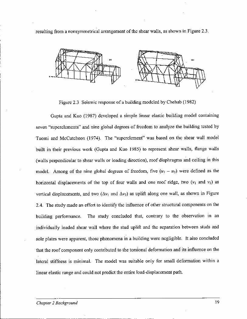
resulting from a nonsymmetrical arrangement of the shear walls, as shown in Figure 2.3.
Gupta and Kuo (1987) developed a simple linear elastic building model containing
seven "superelements" and nine global degrees of freedom to analyze the building tested by
Tuomi and McCutcheon (1974). The "superelement" was based on the shear wall model
built in their previous work (Gupta and Kuo 1985) to represent shear walls, flange walls
(walls perpendicular to shear walls or loading direction), roof diaphragms and ceiling in this
model. Among of the nine global degrees of freedom, five (u\ - us) were defined as the
horizontal displacements of the top of four walls and one roof ridge, two (vi and v2) as
vertical displacements, and two (Avi and Av 2) as uplift along one wall, as shown in Figure
2.4. The study made an effort to identify the influence of other structural components on the
building performance. The study concluded that, contrary to the observation in an
individually loaded shear wall where the stud uplift and the separation between studs and
sole plates were apparent, those phenomena in a building were negligible. It also concluded
that the roof component only contributed to the torsional deformation and its influence on the
lateral stiffness is minimal. The model was suitable only for small deformation within a
linear elastic range and could not predict the entire load-displacement path.
Figure 2.3 Seismic response of a building modeled by Chehab (1982)
Chapter 2 Background 19

Figure 2.4 Global degrees of freedom for house model by Gupta and Kuo (1987)
Schmidt and Moody (1989) developed a static model (RACK3D) by using a simple
energy approach to analyze three-dimensional wood light-frame structures. This model
extended the previous work on woodframe shear walls by Tuomi and McCutcheon (1974),
combined with nonlinear fastener models developed by Foschi (1977) and McCutcheon
(1985) to predict the nonlinear response of structures to lateral monotonic loading. In this
model, all the walls with the same height were connected to a rigid roof diaphragm at a single
point, which was located at the mid-span of a shear wall. Walls carried only in-plane racking
forces without considering out-of-plane bending or torsion. The model was verified with the
tests conducted by Tuomi and McCutcheon (1974) and Boughton and Reardon (1984), in
which all the test specimens were single storey houses. The results indicated reasonable
predictions in loads and deformations. The load sharing among walls and torsional motion of
the building due to eccentric load condition were also studied. The deformations in the shear
walls in this study were limited to 0.1 in (2.54 mm) and 0.2 in (5.08 mm). Within this range,
the nonlinearity of the structure was not significant.
Kasai et al. (1994) used ANSYS finite element software to statically analyze a one-
storey light-frame house, tested by Phillips (1993). In the model (Figure 2.5), the roof and
floor systems were considered to be linear and were represented by superelements, while
Chapter 2 Background 20
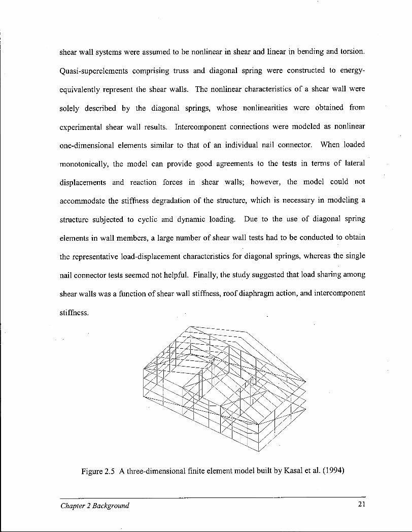
shear wall systems were assumed to be nonlinear in shear and linear in bending and torsion.
Quasi-superelements comprising truss and diagonal spring were constructed to energy-
equivalently represent the shear walls. The nonlinear characteristics of a shear wall were
solely described by the diagonal springs, whose nonlinearities were obtained from
experimental shear wall results. Intercomponent connections were modeled as nonlinear
one-dimensional elements similar to that of an individual nail connector. When loaded
monotonically, the model can provide good agreements to the tests in terms of lateral
displacements and reaction forces in shear walls; however, the model could not
accommodate the stiffness degradation of the structure, which is necessary in modeling a
structure subjected to cyclic and dynamic loading. Due to the use of diagonal spring
elements in wall members, a large number of shear wall tests had to be conducted to obtain
the representative load-displacement characteristics for diagonal springs, whereas the single
nail connector tests seemed not helpful. Finally, the study suggested that load sharing among
shear walls was a function of shear wall stiffness, roof diaphragm action, and intercomponent
stiffness.
Figure 2.5 A three-dimensional finite element model built by Kasai et al. (1994)
Chapter 2 Background 21
In 1995, Foschi developed a three-dimensional finite element diaphragm analysis
program (DAP-3D) for a project carried out at the University of Western Ontario (UWO) to
examine the performance of typical wooden houses subjected to wind loads (Case and
Isyumov 1995). The test houses were composed of vertical shear walls and pitched roofs
with a reduced-scale of 1:100. The wind loads were applied to houses by the turbulence
generator at the Boundary Layer Wind Tunnel Laboratory of the UWO. The program, which
modeled the wood components linear-elastically, was used to obtain influence coefficients
for reaction forces at the foundation, structural displacements, and nail forces. The data was
then compared with National Building Code of Canada (NBCC) code values.
In a project funded by the Forest Renewal B C (FRBC), a finite element program,
P A N E L , was developed by Foschi (1997). This program contained many features that either
were required in a three-dimensional structural analysis or could be expanded from a two-
dimensional space into a three-dimensional space, although it was designed for analyzing
two-dimensional light-frame structures under static monotonic loading. For example, in the
program, each node was provided with seven degrees of freedom (three translations and three
rotations plus one twist), and by using plate element, the out-of-plane deformation can be
calculated. The program allowed multiple and combined loading conditions to be applied to
a diaphragm simultaneously. These loads included distributed loads acting normal to the
panel plane and concentrated loads acting in the panel plane. Some of these loads can be
incremental while the others were constant. In the panel to frame connections, besides the
lateral deformations, the withdrawal and rotation of a nail connector were also analyzed. The
program also tried to consider as many as possible variables affecting the behaviour of a
structural component, which provided generality in the evaluation of the response of different
Chapter 2 Background 22

panels with different constructions. A diaphragm can have sheathing panels on both sides
with different material properties. The analysis was also applicable to diaphragms with
openings. It was the first light-frame structural analysis to consider the influence of
insulation material filled between the two sheathing layers. A l l these features combined with
the structure of the model in the P A N E L program laid a foundation on which the models in a
three-dimensional space can be developed. The major limitation of the P A N E L program was
that the behaviour of nail connections was predicted based on the experimental backbone
functions. Therefore, it could be used only for monotonic pushover loading conditions.
In 1997, Tarabia and Itani presented a three-dimensional dynamic model for light-
frame wood buildings. The diaphragms in the model were divided into a few sections with
four master nodes for each section. These master nodes were located along the boundaries of
a diaphragm connecting to other diaphragms and internal degrees of freedom were condensed
out during the solution. The model did not consider out-of-plane deformations in the
diaphragms and assumed that the panels can deform in shear only. Nail connections between
the panel and frame members were modeled as two perpendicular decoupled nonlinear spring
elements with the hysteresis behaviour proposed by Kivell et al. (1981). This connection
model, similar to other connection models discussed in Section 2.2.5, used a few linear
functions to represent the connection's loading history. This study covered the effect of
aspect ratio on the rigidity of horizontal diaphragms, load distribution mechanisms,
asymmetric lateral-load resisting systems, and transverse walls. It was found that the rigidity
of the horizontal diaphragm was influenced by the aspect ratio. As the aspect ratio increased,
the rigidity of the diaphragm decreased. The amount of seismic forces carried by the
partition walls depended on the length and rigidity of roof diaphragm, and the stiffness and
Chapter 2 Background 23

aspect ratio of the partition walls. The study also concluded that using the asymmetric
lateral-load resisting system induced torsional moments in the building and the transverse
walls can carry a significant amount of shear forces generated from the torsional moment.
More recently, a hybrid approach combining deterministic and stochastic methods to
model light-frame buildings was proposed (Kasai et al. 1999). In this approach, a
complicated 3D building was first subjected to a very simple loading history that produced a
cyclic response. By using system identification techniques, the response was then fitted into
a simplified two-dimensional model, for example, a shear-building model with a general
differential hysteresis developed by Foliente (1995), with only a few degrees of freedom.
This shear-building model was based on the assumptions that (1) the entire floor systems
were infinitely rigid as compared to the columns, and (2) the rigid floor systems remained
horizontal during the ground motion. Stochastic analysis or Monte Carlo simulations could
be applied to the model, where the system properties and loads were treated as random
variables, under an ensemble of loads to determine a possible range of loading scenarios.
Finally, the resultant response statistics would be used to describe the behaviour of the actual
3D buildings. From the above descriptions it can be seen that the model was only capable of
predicting the load-displacement behaviour of a particular three-dimensional building based
on the behaviour of each individual component. It did not provide any information on the
system effects, such as torsional motion, load sharing, and so on.
A 3D dynamic time-history analysis was carried out in Canada (Ceccotti et al. 2000)
to investigate the influence of diaphragm flexibility on ultimate state of a four-storey
symmetric wood frame building. A three-dimensional non-linear dynamic analysis program
(DRAIN®-3D) with a pinching nail model was used in the study. It was concluded that the
Chapter 2 Background 24
flexible floors could reduce the capacity of the wood building by approximate 15% when
compared to the rigid floor case. The study was used to quantify the action reduction factor
(ARF) in design codes, whereas the influence of varied relative stiffness ratio of floor
diaphragms and shear walls on building performance including load sharing and building
deformation was not addressed.
2.2.2. Experimental studies
Experiments of full-scale light-frame houses were seldom performed in a laboratory
environment in the early stages of study of wood light-frame building due to technical and
physical difficulties. Polensek (1983) summarized a few of such experimental studies in a
span of more than twenty years by Dorey and Schriever (1957), Hurst (1965), Yokel, et al.
. (1972), Tuomi and McCutcheon (1974), and Yancey (1979). These studies usually involved
simple and symmetric building specimens, loaded statically. None of these tests related with
numerical analysis, and often the test results were incomplete. Entering 1980s, more efforts
were made on experimental studies of full scale light-frame buildings by Hirashima, et al.
(1981), Boughton (1982-1988), Sugyiama et al. (1988), Steward et al. (1988), Yasumura et
al. (1988), Jackson (1989), and Phillips et al. (1993). These studies tried to understand the
structural performance and characteristics of a complete wooden building. Some of them
served as a verification of the design values. In general, the tests consisted of several stages
at which the structural components were added to the building gradually to determine the
influence of the components on structural behaviour of the building. Investigations of lateral
load carrying capacity and drift, load sharing and interaction among components, and
variations in structural materials in a full-scaled house were the main objectives. Then the
test buildings were developed in irregular arrangement of interior walls and openings with
Chapter 2 Background 25
floor and roof installed. The level of the houses ranged from one storey to three storeys. In
most tests, only static lateral loads were applied to the tested specimens. In some cases,
cyclic lateral loads were applied to simulate wind loads.
One of the most prominent and comprehensive ongoing projects investigating light-
frame buildings under dynamic earthquake ground motion is the CUREE-Caltech wood-
frame project (Hall 2000). This is a $6.9 million F E M A (Federal Emergency Management
Agency)-funded effort administered by California Office of Emergency Services. The goal
of the project is to improve the seismic performance of wood-frame construction through
development of cost-effective retrofit strategies, changes in design and construction
procedures, and education. The project started in 1998 and is expected to be finished in three
to four years. In the Testing and Analysis, one of five elements of the project, the plan
incorporates five main research tasks, centering on the shake table tests of large-scale wood-
frame systems (Filiatrault et al. 2000). The test specimens include conventional wood light-
frame structures from simplified box-type models (Task 1.1.3), full-scale two-storey single
houses (Task 1.1.1) to multi-storey apartment buildings (Task 1.1.2). The simplified box-
type models (Task 1.1.3) have been tested at the University of British Columbia as part of the
work in this thesis. It is an integral component of a parallel study funded by the Forest
Renewal BC (FRBC). The test results will be described in detail in the subsequent chapters.
In Task 1.1.2, a two-storey single-family house of 4.88 m x 6.10 m (16 ft x 20 ft) in plan
(Figure 2.6), following current California residential construction practice, was tested under
the 1994 Northridge earthquake ground excitations. In 2000, an International Benchmark
was being organized in which researchers and design professionals, inside and outside
California, as well as the international communities were invited to blind-predict the inelastic
Chapter 2 Background 26
seismic response of this tested two-storey wood-frame building. This provided a unique
opportunity to assess the capacity of available numerical models incorporating widely
different levels of sophistication and to foster cooperation between the CUREE-Caltech
Woodframe Project and other related research activities. In this blind prediction, five
international teams completed the benchmark exercise by adopting different types of
numerical models. The results ranged from poor to excellent when compared to the test
results (Folz et al. 2001). A l l teams modeled the test building in multiple phases. In general,
the test data of the connections between panel and frame were first fit into a hysteresis model
to develop a full shear wall model. This shear wall was subsequently reduced to a single
spring element. These nonlinear spring elements were then assembled to represent the entire
building. The roof and floor diaphragms were assumed to be rigid, which was validated with
the test results. The study concluded that almost all commercially available general purpose
structural analysis programs did not contain hysteresis models that are suitable for wood
fasteners or wood components. It was also found that the appropriate level of viscous
damping to be used in the modeling was difficult to determine. The reason was that at low
levels of structural response, the hysteresis elements may not dissipate any significant
amount of energy, whereas at high levels of structural response, viscous damping may be
entirely overshadowed by the energy dissipation of hysteresis mechanisms that were
activated in the structure. Each participating team commented that the nonlinear dynamic
analysis was a time-consuming task, even i f an oversimplified structural model was used.
This benchmark study indicated that a greater research effort is required to advance the
knowledge base of numerical models for woodframe structures, before these analytical tools
can be used effectively in the seismic design process.
Chapter 2 Background 27

Figure 2.6 Two-storey building test in the CUREE-Caltech wood-frame project (Folz et al.
2001)
The Earthquake 99 Project was another major large-scale study of wood light-frame
buildings under earthquake loading conditions, which was designed and managed by T B G
Seismic Consultants and Simpson Strong-Tie in collaboration with the University of British
Columbia (Pryor et al. 2000). The project was to investigate the seismic performance of
narrow Simpson Strong-Walls and conventional shear walls complying with the 1997
Uniform Building Code of the United States by testing a series of one- and two-storey
buildings (Figure 2.7). In these buildings, the primary lateral force resisting system consisted
of either four conventional shear walls, 1.22 m (width) by 2.44 m (height), or four Simpson
Strong-Walls, 0.61 m (width) by 2.44 m (height), installed at both ends of two exterior walls
parallel to the shaking direction. A specially designed unidirectional shake table was
constructed to accommodate the test specimens with plan dimensions of 6.10 m by 7.62 m
Chapter 2 Background 28

(20 ft by 25 ft) and an inertial weight of 200 kN (45,000 lbs). The input earthquake histories
were the Canoga Park record and the Sherman Oaks record of the 1994 Northridge
earthquake. The peak ground acceleration (PGA) of the Canoga Park record was scaled up
20% from the original one to 0.50g and was then further increased after the first test to reach
0.63g. The PGA of the Sherman Oaks record was 0.45g. Preliminary observations indicated
that the permanent drift in the building using Simpson Strong-Walls was substantially
smaller than that using the conventional shear walls. The tests also showed that the Simpson
Strong-Wall system could sustain multiple large earthquake events better than its counterpart.
(a) One-storey test building
Chapter 2 Background 29

(b) Two-storey test building
Figure 2.7 Shake table tests of Earthquake 99 project
It is worth mentioning that in the past few decades, a large number of wood building
tests have been carried out, both statically and dynamically, in Japan. Most of these tests
were focused on the traditional Japanese post-beam and bracing systems. Only a small
number of tests were carried out to study the North American 2><4 construction. After the
1995 Kobe earthquake, a number of Japanese researchers conducted shake table tests to study
the dynamic performance of shear walls (Yamaguchi and Minowa 1998), wooden houses
(Kohara and Miyazawa 1998, and Ohashi et al. 1998), and wood-framed houses with bracing
systems (Tanaka et al. 1998). These tests on the structural components or the traditional
Japanese building systems are not discussed in this thesis, which specially focuses on light-
frame buildings.
Chapter 2 Background 30
2.2.3. Studies on the system effects in building
A light-frame building is an assembly of two-dimensional components, joined by
connectors. It is inevitable that load sharing and interaction among the components exist
when the building is loaded, which is the major distinct difference in behaviour of a building
from the individual components. Identifying the load sharing as well as the load paths,
however, is not an easy task, because it can be influenced by many factors. In early studies,
this fundamental phenomenon was largely ignored since the emphasis was placed mainly on
isolated building components. This issue has gradually attracted researchers' attention, along
with the development of analyses and experiments of building systems, but no systematic
study has been conducted to provide a general understanding of the load sharing mechanism.
The major factors believed to affect the load sharing among the components include stiffness
of wall components, rigidity of floor/roof systems, mass distribution within the building
(under dynamic load), boundary conditions (how the walls being fixed to the foundation),
and inter-component connections.
In a full-scale house test under cyclonic wind loads, Boughton (1988) concluded that
the load did not always follow paths through the major structural components and the
supporting boundary conditions of the components affected the stiffness, ultimate load, and
failure characteristics of components under test. This testing also suggested that the
components behaved differently in a building test from the prediction of component model.
The design methods based on the component studies may give unconservative results;
however, this could be compensated by redundancy of the whole system.
A comprehensive study investigating the system effects in buildings was conducted
by Phillips et al. (1993). With sufficient instrumentation, the tests provided extensive data,
Chapter 2 Background 31

which were often used by other researchers in later studies. The overall dimensions of the
test building were 4.88 m wide by 9.75 m long (16 ft by 32 ft) (Figure 2.8). The roof trusses
spanned in the long direction of the building. The house had three separate rooms with doors
and windows in different locations to create an asymmetric structural layout. Concentrated
loads were applied to the top corners of the shear walls. Considerable efforts were made to
instrument the building to obtain the internal force distributions. Eight load cells were
embedded into shear walls to measure the horizontal and vertical loads in each shear wall.
The gross displacement at the top of each shear wall, the slip at the base of each shear wall,
the uplift of the loaded side, and the transverse displacement of the building were measured
by linear variable differential transformers (LVDTs). The study found that the roof
diaphragm had contributed significantly to lateral load sharing among the vertical shear walls
of the building. The roof behaviour was much closer to a completely rigid response than a
completely flexible response, as was typically assumed for the design of light-frame
buildings. The observed load distributions were a function of the shear wall stiffness, wall
position within the building, and the size of the building. This finding was supported by the
evidence observed in other tests (Stewart et al. 1988, Yasumura et al. 1988). It was
concluded that the walls perpendicular to the loading direction carried a percentage of the
lateral load applied to the building, which was localized around the connection of the
transverse walls with the shear walls. The percentage varied between 8% and 25%, and
decreased with increasing applied load. The transverse walls did not contribute to load
sharing among the shear walls. Similar results were also obtained by the tests conducted by
Sugiyama et al. (1988) and Jackson (1989).
Chapter 2 Background 32

9754 mm
Figure 2.8 Three-dimensional view of test structure (Phillips 1993)
A study was carried out at Lund University (Andreasson 1999) to investigate
influences of the diaphragm interaction on the distribution of dead load in a wood frame
system. The author questioned the present design approach, in which all structural
components were designed separately, with no consideration of load sharing in the three-
dimensional structure because the approach assumed that the overall performance of a
structural system subjected to a horizontal loading can be simplified to two-dimensional
analyses, where only the shear walls were active. In the study, a static non-linear finite
element model was developed using ANSYS software, of which the multi-storey timber
frame building was idealized as horizontal and vertical diaphragms connected by springs.
The investigation was focused on the distribution of dead load along shear walls and the
transfer of dead load via transverse walls. The study concluded that the distribution of dead
Chapter 2 Background 33
load and the uplift load at anchorage were affected by sheathing configuration, wall length,
panel dimension, anchorage stiffness, dead load magnitude, and number of storeys. For
example, the dead load transferred to the anchorage in a two-side sheathed shear wall was
larger than that in a single-side sheathed shear wall. It was also true in a longer shear wall
vs. a shorter shear wall. These results indicated a smaller uplift in the end studs due to
increased share of dead load. It was found that the distribution of dead load among studs was
not linearly increased with increasing dead load. In a multi-storey building, it seemed that
the top floor obtained the largest potion of dead load while the ground floor obtained the
smallest, which implied that the multi-storey system acted as one diaphragm over all storeys,
and its total load capacity was not a simple multiplication of the load of one storey by the
number of storeys.
Foliente et al. (2000) presented preliminary test results of an L-shaped wood frame
house in Australia. The primary objectives of the project were to improve the understanding
of load sharing and distribution within a light-frame wood building and to generate data
needed to validate building analytical models (Figure 2.9). The results from the first phase
tests indicated a significant load sharing within the whole building. For example, Walls 3
and 4 took a significant in-plane load when the load was applied to Wall 2 only. This load
transfer was partially due to the end walls (perpendicular to shear walls) and partially due to
the roof system. Because Wall 3 was not connected to the roof trusses, the load transferred
to Wall 3 was only via the end walls. This observation differed from that of the tests by
Phillips et al. (1993), which concluded that the transverse walls in a house did not contribute
to load sharing among the shear walls, as discussed previously. At this stage, only static tests
within elastic range were performed. Further study on more loading configurations, the
Chapter. 2 Background 34

stiffness of roof diaphragm, and the torsional stiffness of the whole house is under way.
Dynamic testing is also scheduled. Finite element analysis will be in place to conduct
parametric and sensitivity studies. 1 * C A A A m^n
W9
W1
W7 we
W2\ W3
W8
W4
WS
(a) Test model framing (b) Plan view and wall numbering
Figure 2.9 L-shaped test house (Foliente et al. 2000)
2.2.4. Testing methods
The most commonly used testing methods in investigating the structural performance
of wood light-frame buildings fall in three categories: static monotonic testing method, quasi-
static or cyclic testing method, and dynamic testing method. Briefly, they are described as
follows.
Static monotonic testing method - In experimental study of a wood system, static
loading is usually first applied. The approach is fairly simple to provide basic static strength
and displacement characteristics of the structure. It is useful because most seismic design
codes require that a building be designed to resist specified equivalent static forces. Under
static loading, the behaviour of the system can be described by a simple load-displacement
Chapter 2 Background 35

relationship (Figure 2.10).
re o _ i
Displacement
Figure 2.10 General load-displacement relationship of a wood structure
Unlike steel materials, wood materials do not have an obvious yield point, and the
load-displacement relationship presents nonlinearity. To characterize the structures,
important parameters, such as stiffness, ductility, ultimate strength, and displacement, have to
be defined. Ductility is thought to be the most important quality because it is the ability to
deform beyond the elastic limit without substantial reduction in strength and has been used as
a criterion in establishing inelastic design response of wood buildings. Most of design
procedures (codes) rely on the results from these simple static push-over tests and models on
the structural components. Sometimes, the results can be misleading, because
(1) the behaviour of wood structures is heavily loading history dependent, which means that
the performance of a structure under static loading may not be the same as the
performance under seismic loading; and
(2) the good performance (e.g. high ductility) of individually tested components does not
imply the same performance of an entire building under the same loading condition.
Cyclic testing method - As an important step toward a better understanding of the
performance of wood structures under wind and seismic loading and improvement in seismic
Chapter 2 Background 36

design methods, a quasi-static or cyclic test is carried out. Cyclic tests are still within the
static region, because the loading speed is so low that no dynamic effect or inertia forces can
be produced. It can be seen from the literature review that wind loads applied on wood
structures are usually simulated as cyclic loading because of their much lower frequencies
and cyclical nature. Under cyclic loading, the load-displacement relationship of a wood
based structural system is governed by hysteresis characteristics (Figure 2.11) which have
been identified by many researchers (Foliente 1995):
(1) nonlinear, inelastic load-displacement relationship without a distinct yield point;
(2) progressive loss of lateral stiffness in each loading cycle or stiffness degradation;
(3) loss of strength when cyclically loaded to the same displacement level or strength
degradation; and
(4) pinched and usually asymmetric hysteresis loops.
Displacement
Figure 2.11 General hysteresis loops of a wood structure with a monotonic push-over curve
One of the purposes of doing cyclic tests is to understand the energy dissipation
mechanism in a wood structure. The area of hysteresis loops is used as a measure of the
energy dissipated by the structural components when subject to a cyclic loading. Clearly,
wider loops will be beneficial to the structure, because more energy can be dissipated to
Chapter 2 Background 37
postpone the structure failure. Most nailed wood components show, however, pinched or
area-reduced hysteresis loops, meaning a reduced energy dissipation capability or reduced
hysteresis damping of the structure. This conclusion seems inconsistent with the good
performance of the wood structures. Researchers have found that the ability for a wood
structure to sustain a larger deformation without significant deterioration of the strength
(higher ductility) appears to be much more significant. It is believed that the pinched loop as
well as the stiffness and strength degradation results from the crushing of the wood around
the nail shank and slipping of the nail in panel and frame members. It is noted that the
energy dissipation capacity of a structure computed from the area of hysteresis loops is
highly influenced by the type of loading history (He et al. 1998). Therefore, the energy
dissipation capacities of wood structures tested under different loading histories may not be
comparable.
In cyclic tests, several different loading protocols are available, including A S T M -
SPD (1993, 1996), C E N (1995), FCC-Forintek (1994) and others used in Australia and New
Zealand. When ASTM-SPD and FCC-Forintek protocols were used, the tests often resulted
in low cycle fatigue fracture in the nails connecting panels and frame members, which was
not commonly observed in wood buildings subjected to earthquakes or dynamic tests. Under
C E N short protocol only a few cycles (usually three) with high amplitude were applied,
which caused unrecoverable damage in nail joints at the very beginning of the test; therefore,
the test results were difficult to justify. Test results from different protocols were not directly
comparable because of the difference in defining parameters. A project was under way to
develop a consistently recognized international standard for cyclic load testing of wood-
based structures (Karacabeyli 1996).
Chapter 2 Background 38
Dynamic testing method - Usually a dynamic test is performed on a shake table with
the input of previous earthquake records as ground motion excitations. The excitations could
be applied in one or multiple directions depending on the research needs and the capacity of
the test facility. The test specimen is tied to the table, carrying a certain amount of mass on
its top to generate the required inertial forces. Dynamic testing is preferred, because it
reveals the actual behaviour of a system during an earthquake and provides more information
than a static or quasi-static test to help better understand the seismic characteristics of a wood
light-frame building. Of course, dynamic testing is more costly and more technically
demanding. The scale of a test is also restricted in the limitation of dimensions and payloads
of a shake table. In a dynamic test, besides the structural considerations of the test specimen,
the earthquake records and inertial mass should be carefully selected. If required, an
earthquake record could be modified to obtain the right acceleration amplitude, frequency
components, and duration. The mass on the top of structure will decide the load applied to
the structure under the chosen earthquake excitation. Using properly installed
instrumentation, the entire response history of a test system under specified excitation can be
recorded. A forced vibration test is usually applied to the test system before and after the
main test to determine the natural frequencies and the corresponding mode shapes.
Another type of test, called pseudo-dynamic test, is often performed. The pseudo-
dynamic test is performed quasi-statically and provides a realistic simulation of the response
of structures exposed to dynamic loadings. In the pseudo-dynamic test, a record of an actual
or artificially generated earthquake ground acceleration history is given as input data to the
computer. The horizontal displacements of diaphragms, such as floors or roofs at which the
mass of the building can be considered to be concentrated, are calculated for a small time
Chapter 2 Background 39
step. These displacements are then applied to the structure by servo-controlled hydraulic
actuators fixed to the reaction wall. The forces necessary to achieve the required
deformation are measured and then sent to the computer, combined with analytically
modeled inertial and viscous damping forces, for the next step of the calculation. The
pseudo-dynamic test method offers the possibility to test very large models and to monitor
closely the progression of damage in the structure. Due to high equipment costs, however,
the number of suitable hydraulic actuators is a serious limitation, which limits the number of
degrees of freedom that can be tested in the laboratory. The method is especially useful for
confirmatory tests in full-scale where exact material and construction details can be
reproduced, or when multi-point input loading is required.
2.2.5. Connection models
The behaviour of the nail connections between sheathing panels and frame members
is generally accepted to be a governing factor in defining the overall performance of the
building component. Under dynamic loading, the hysteresis properties of a connection play a
central role in deciding its energy dissipation characteristics during the deformation history.
It is essential, therefore, in almost every analytical study, to study and model the load-
displacement relationship and the hysteresis loops. Foschi (1974, 1977, Figure 2.12)
published a model representing the monotonic load-displacement characteristics of nail
connections in wood diaphragms. Many researchers used and modified this model to suit
specified testing conditions.
Chapter 2 Background 40

Eo A
Figure 2.12 Nail load-displacement model (Foschi 1974, 1977)
Stewart et al. (1988), Dolan (1989), Kasai and X u (1997), and Davenne et al. (1998)
also modeled the hysteresis loops of nailed wood joints in shear wall or diaphragm systems
(Figure 2.13). A particularly notable procedure was developed by Baber, Noori and Wen
(1981, 1985) and modified slightly by Foliente (1993), using 13 parameters to account for
yielding, pinching, strength, and stiffness degradations of a wide variety of possible
combinations of materials and joint configurations. Krawinkler et al. (2001) also developed
a connector loading protocol for the CUREE-Caltech Woodframe Project.
Chapter 2 Background 41

(c) (d)
Figure 2.13 Modeled hysteresis loops of nailed wood joints by various researchers
(a) Stewart, Dean and Carr's model, 1988; (b) Dolan's model, 1989;
(c) Kasai and Xu's model, 1997; and (d) Davenne et al.'s model, 1998.
A commonly used approach in this type of modeling was to fit experimentally
observed characteristics of the specified wood joint, with the model basically being a post-
test product. The model can then predict the performance of a joint for which the model was
developed under static monotonic and cyclic loading because usually the loading paths have
very regular patterns. However, it was noted that these hysteresis models could not provide
satisfactory results when the material properties and joint configurations varied from the
modeled one. The fitted models may not necessarily predict the hysteresis behaviour and
energy dissipation of a structure subjected to dynamic loading under which its hysteresis
loops were no longer nicely shaped.
A n alternative that can be used in modeling the connection was using a general,
mechanics-based approach. This type of model was developed (Foschi 2000) and
implemented into a subroutine HYST (as it was usually called) for the calculation of
hysteresis loops in mechanical connectors from basic material properties of the connector and
the embedment characteristics of the surrounding wood medium. This approach considered a
Chapter 2 Background 42

nail connector as an elastic-plastic beam acting on wood, modeled as a nonlinear medium
which only acted in compression, permitting the formation of gaps between the beam and the
medium. The model can then develop pinching as gaps were formed, and thus the energy
dissipation in a connection's deformation history can be accurately represented. The HYST
as a subroutine could be inserted into any program requiring calculations of nail forces. The
subroutine itself was a finite element program calculating the coordinates of the hysteresis
loop at each time step, by solving the nonlinear problem of the structural response to the
imposed history. Calculating the true response involved a complicated three-dimensional
problem, but it can be estimated from basic stress-strain information on the structural
member (nail) and from a simple representation of the nonlinear behaviour of the medium
(wood) surrounding that member. A beam finite element formulation was used for the
member, using high order interpolating shape functions to reduce the number of required
elements. The main advantage of this approach was that, starting from basic material
properties, it automatically adapted to any input displacement history. Instead of calibrating
parameters, to some of which it may be difficult to assign a physical meaning, the approach
used constants with which engineers are more familiar, such as moduli of elasticity, yield
stress, etc (Foschi 2000). Because the model can well reflect the actual behaviour of general
connections in a more reliable manner, it was implemented into the programs developed in
this thesis work to make the predictions under cyclic and dynamic loadings possible. It
should be noted that the model is more computational intensive in a dynamic analysis when
comparing to other curve-fitting nail models because it needs to be invoked for each nail or
key nails within a nail line for each time step. The finite element iterative procedures are
called to solve this nonlinear problem. It is estimated that more than 90% of C P U time is
Chapter 2 Background 43

spent on the calculation of nail connection behaviour in the programs developed in this study.
This shortcoming should not be considered serious when the methods discussed in Chapter
10 are employed. In addition, the computational effort is amply compensated by increased
model reliability for dynamic analysis (Foschi 2000).
In this chapter, the literature relating modeling and testing of three-dimensional wood
frame constructions is overviewed and some important issues are discussed. It is evident that
most of previous work was focused on two-dimensional structural components or simplified
three-dimensional buildings. In recent years, the study has shifted to three-dimensional
buildings and some progress has been made. Based on the research needs in three-
dimensional light-frame structures, this thesis work extends from previous research efforts to
develop numerical models. The objective is to use these models as practical tools in
predicting and understanding the behaviour of three-dimensional wood light-frame buildings
under seismic loadings.
Chapter 2 Background 44

CHAPTER 3
THE STRUCTURAL MODEL
The first step in finite element structural analysis is the idealization of the actual
structure (physical model) into a mathematical model. This idealization must consider the
configurations and properties of the structural members, the loading conditions, and the
boundary conditions. The structural members need to be represented by certain types of
elements and their material properties have to follow some idealized rules. The complex
loading conditions of the. structure will be simplified, for example, as concentrated and
distributed forces. The fixities of the structure to the foundation or the connections to the
support are idealized as boundary conditions with or without prescribed displacements. A
proper idealization of these components has significant influence on how the solution of a
finite element analysis closely converges to the actual result. In this chapter, only the
idealizations of structural members and material properties are discussed. The loading
conditions and boundary conditions should be recognized in the individual cases.
Three types of elements are used in the model development to represent the members
in wood light-frame buildings. These elements are panel elements, frame elements, and
connection elements. The panel elements are approximated as thin plate elements in a three-
dimensional field. Each frame element consists of four sides with each side modeled as a
three-dimensional beam element. In this study, a general mechanics-based connection
Chapter 3 The Structural Model 45
model, HYST (Foschi 2000), is introduced into the newly developed finite element
programs. Using this model allows the finite element programs to perform cyclic and
dynamic analyses by calculating hysteretic loops in mechanical connections from basic
material properties. The connection element in HYST models the behaviour of a nail and the
areas of the panel and frame members that surround the nail. These areas are represented by
non-linear spring elements. The nail itself is assumed to obey an elasto-perfectly plastic
constitutive relation. The approach used in this model overcomes the disadvantages of
commonly used empirical connection models, in which an algorithm is added to trace
hysteresis loops fitted to experimental data of a given connection.
In the finite element approximation, a basic element unit contains the above-
mentioned three types of elements in a sandwich pattern as shown in Figure 3.1. Each
element unit has four nodes with six nodal degrees of freedom and one element degree of
freedom (Figure 3.2). The nodal degrees of freedom are the three translations in x, y and z
directions (u, v, w), and the three rotations about x, y and z axes {Rot-x, Rot-y, Rot-z). The
element degree of freedom is the twist in x-y plane (wxy). Connection elements have three
degrees of freedom at each node (u, v, w).
A l l three types of elements used in the model are isoparametric elements. An element
is isoparametric i f one set of nodes and shape functions, represented by natural coordinates £
and r|, can be used to define both nodal displacements (w, v, w) and nodal coordinates (x, y,
z). The isoparametric elements are useful because, by selecting appropriate shape functions,
the sides of the elements between two nodes can be curved to closely model the deformation
of real structures. Those elements have proved to be more effective and accurate than the
traditional triangular and rectangular elements by using fewer elements.
Chapter 3 The Structural Model 46
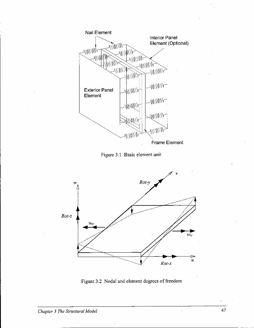
Nail E lemen t
F rame E lemen t
Figure 3.1 Basic element unit
Figure 3.2 Nodal and element degrees of freedom
Chapter 3 The Structural Model Al

3.1. Panel element
The panel elements are represented by thin plate elements, which can be loaded by in-
plane and/or out-of-plane forces and can deform in three-dimensional space. Under the
action of both types of loads, the deflection of plate can be large in comparison with its
thickness, but is still small when compared with the other dimensions. Therefore, the
analysis has to be extended to include the strain of the middle plane of the plate (Timoshenko
1959, Ch. 13).
3.1.1. Assumptions
The following assumptions are applied to the plate element:
(1) The normals to the middle plane remain normal to it during deformation (Bernoulli-Euler
Assumption),
(2) The change in the thickness of plate element is negligible,
(3) The buckling deformation of plate element is modeled by considering bending deflection
amplifications due to the effect of axial compressive loads (large deflection),
(4) The plate element has a linear elastic material property and obeys orthotropic stress-
strain relationships, and
(5) The extensional or compressive deformation of plate element is linear and the deflected
shape of the element is defined by cubic polynomials.
3.1.2. Geometric and physical relationships
Based on assumptions (1), (2), and (3), when the plate element is subjected to axial
(tension or compression) and bending deformations in its x-y plane, the displacement in z
direction is only a function of x and y. The displacement fields in a plate element are,
therefore, determined as the following,
Chapter 3 The Structural Model 48

dw us = u- z—
dx dw
v = v - z — dy
ws =w(x,y)
(3.1)
where
us, vs, ws = the small displacements of a point in the middle plane of the plate
element during deformation in the x, y and z directions, respectively.
u, v = the small displacements caused by axial deformation only in the x and
y directions, respectively.
Considering a small section AB of the middle plane of the plate element in x direction,
the strain due to displacements u and w, referring to Figure 3.3, is
ds - dx _ ds j _ dx dx
du\2 (dw^2 -ll/2
1 + — dx j + ydx j
-1 (3.2)
Using Taylor series expansion and ignoring third and higher order terms, the strain in
Equation (3.2) approximates to
2 ~du 2— +
dx
du lfdw} = — +
dx 2 \ dx,
(du\ [dx,
2
+ 'dw1
ydX; ydu (du\2 (dw^2
dx \dx Kdxj + . . . _ !
(3.3)
Chapter 3 The Structural Model 49

B'
u
A
ds A'
t dw ,
dx dx
\ u
A
dx+du u
A B
dx du ,
u H dx dx
Figure 3.3 Middle plane extension of plate element
The strain of the middle plane due to bending is
d2w e = - z — -
dx2
Thus the total normal strain in x direction is obtained
d2w 8 = e + 8 = 1—
* * ' dx 2
8u 1 fdw^2 a2-ydxj dx2
In the same way, the normal strain of the middle plane in y direction is
( dw\2
t , 9v 1 8 , + 8 , = + —
8ZW
(3.4)
(3.5)
(3.6) -> ~y'~y dy'2{dy) dy2
The shear strain in the middle plane of a plate element also results from axial
deformation and bending. The component of shear strain due to the displacements u and v is
(Equation (3.1) and Figure 3.4(a))
du, c V du dv . d w y' =—s- + — = — + 2z dy dx dy dx dxdy
(3.7)
Chapter 3 The Structural Model 50

The component (yi + 72) of shear strain due to the deflection in w direction can be obtained
from Figure 3.4(b). Vectors a and b, representing deformed edges of the element, are
dx 0
dw . , —dx [dx
and b =
0
dy dw , dy
a • b = a b coset« dxdy sin(90 - a) = dxdy sin(y, + y 2 )
Because
dw dw a»b = dx-0 + 0-dy +—dx—dy
dx dy
then
Y, +Y 2
dw dw dx dy
(3.8)
(3.9)
(3.10)
(3.11)
Adding these two components (3.11) to the components in (3.7), the total shear strain is
du dv dw dw „ d2w yx = — + — + 2z (3.12)
xy dy dx dx dy dxdy
• x
(a) in x-y plane (b) due to deflection in w direction
Figure 3.4 Derivations of shear strain components
The stress-strain relationships of plate element are
Chapter 3 The Structural Model 51
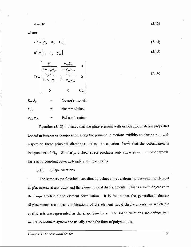
a = De (3.13)
where
eT = k Ey y*y ]
(3.14)
(3.15)
D =
v E xy x
1—V V 1—V V v xy r yx x y xyy yx
VyxEy Ey • V V
xy yx 1 — V V
xy yx
0 0
0
0
r*~I
(3.16)
Ex, Ey
G xy
^xy, Vyx
= Young's moduli.
= shear modulus.
= Poisson's ratios.
Equation (3.13) indicates that the plate element with orthotropic material properties
loaded in tension or compression along the principal directions exhibits no shear strain with
respect to these principal directions. Also, the equation show's that the deformation is
independent of Gxy. Similarly, a shear stress produces only shear strain. In other words,
there is no coupling between tensile and shear strains.
3.1.3. Shape functions
The same shape functions can directly achieve the relationship between the element
displacements at any point and the element nodal displacements. This is a main objective in
the isoparametric finite element formulation. It is found that the generalized element
displacements are linear combinations of the element nodal displacements, in which the
coefficients are represented as the shape functions. The shape functions are defined in a
natural coordinate system and usually are in the form of polynomials.
Chapter 3 The Structural Model 52

The element nodal coordinates in terms of natural coordinates are, referring to Figure 3.5
Ax „ x = xc+—c,
Ay y = yc+Yr[
where
xc,yc
Ax, Ay
coordinates of plate element center,
side lengths of plate element,
variables of natural coordinate system.
The relation between the two coordinate systems is
d d dx a$ 8
, - T 1 . d ' dy • — J
d d dxdy \dipx\\
_2_ Ax 0
0
0 0
— 0 Ay
2 2 0 — —
Ax Ay
d\ d_
d
I Scar, J
where J is Jacobian matrix.
4 (-1,1)
Ay
3(1,1)
(xc,yc)
1(-1,-1) Ax 2(1,-1)
(3.17)
(3.18)
Figure 3.5 Natural coordinate system
In the four-node plate element, let the degrees of freedom vector be
Chapter 3 The Structural Model 53

a T = du, dv, dw, dw, d w.
V dy dx dx dy dxdy' (3.19)
du, dv, ,u4,vA,—± + —±, w 4 ,
dw4 3w4 5 w4 *
5c & dx dy dxdy
And then the displacements represented by shape functions and degrees of freedom are
(3.20) U = TVQJM, + A^ 0 2
f du^ + --- + Nmu4+N0S
( du^ v & J
N l a
V = A)1 V1 + A»
' S O
V dx j + --- + Z 0 7 v 4 +Z 0 8
(3-21)
w = M 0 1 w , + M 0 2
f dwx
ydx j + M
r dw^ 03 v dy J
V>0 dxdy + •
+ M0Uw4 + M 0 1 4 V dx j + M 015 \dy j
rd2w4^ dxdy
(3.22)
= Mja
where
TYoi, Zo/, Mo,- = shape functions.
N 0 > L e shape function vectors.
From assumption (5), which states that the extensional or compressive deformations
along the four sides of plate element are linear and the deflections of the element due to
bending and buckling are in the third order (cubic), a set of polynomials can be constructed
u = aQ+al£) + a2r\ + a^rf + a4r[3 + asfyr\ + afcc\ + a7^r|3
v = b0+b1r) + b£ + bg + bg + b£r] + b£2r\ + b^\
w = c0 + c£ + c£2 + eg + c 4r| + c5-n2 + c 6 n 3 + c7^r| + C£2T\
(3.23)
(3.24)
(3.25) + c£v\2 + c 1 ( £ 3 r | + c.̂ V + cnZrf + cx&\2 + cx£2v? + c 1 5^ 3r| 3
where u and v are related to the first three degrees of freedom and w to the remaining four
degrees of freedom of one node in Equation (3.19). In the construction of shape functions,
Chapter 3 The Structural Model 54

the following derivatives of Equations (3.23), (3.24) and (3.25) are also necessary
du — = a2 + 2<23r| + 3a4r) + afc + 2a£x\ + 3a7^r\ (3.26)
dv = b2+ 2b£ + 3b£2 + b5r] + 2b6fy\ + 3b£2r\ (327)
dw = c, + 2c& + 3c 3^ 2 + c 7 n + 2c8i;Ti + c 9r| 2 + 3ci0E,2r\ + 2c nt>| 2
2 „ 3
+ c12Ti3+3c13^2Ti2+2c14Sr| +3c15S ri
(3.28)
dw ~dr\
= c4 + 2c5r[ + 3c 6ri 2 + c7£, + eg + 2c£r\ + cw^ + 2cxgr\
: 3 „ 2 + 3c 1 2 ^ri 2 +2c13dt3Ti + 3 c I 4 ^ T 1
2 +3c1 5^T!
(3.29)
d2w = c 7 + 2c 8^ + 2c 9ri + 3c 1 0 if + 4c, + 3c 1 2r| 2 + 6c 1 3^ 2r| (3.30)
+ 6c 1 4 ^ 2 +9c 1 5 d l 2 r i 2
Substituting the four pairs of natural coordinates (£, r\) at nodes 1, 2, 3, and 4 shown in
Figure 3.5 to Equations (3.23) - (3.30), respectively, the relations between deformations and
natural coordinates yield
u f e r ^ A a 0 v & T i ) = Bb 0 W ( S , T I ) = C C 0 (3.31)
where
« f e T l ) =
[ldy)i
> v feri) = (dv \dxj
> w
W:
((hi) \dxj rdw^
(d2w^ [{tody),]
i = 1...4 (3.32)
Chapter 3 The Structural Model 55
A , B, and C are coefficient matrices and a 0 , b° and c° are vectors for the unknowns a,, bi, and
ct, respectively.
The vectors a 0 , b ° and c° can be obtained by inverting matrices A , B, and C in
Equation (3.31). Substitute the results of a 0 , b ° and c° into Equations (3.23), (3.24), and
(3.25), respectively. Then, reorder them into the form of (3.20), (3.21), and (3.22). After
considering the Jacobian transformations, the shape functions of plate element are
N0l = 0.25 - 0.254 - 0.375n + 0.125n3 + 0.375^r| - 0.125^r)3
N02 = -0.125(l - 4 - n - r,2 + rf + 4 " + tf - tf ) ^
N03 = 0.25 + 0.254 - 0.375n + 0.125r]3 - 0.375^r| + 0.125^r)3
N04 = -0.125(l + 4 - r, - r,2 + r,3 - 4 r , - Zrf + tf ) ^
N05 =0.25 +0.25^+ 0.375ri-0.125r|3 + 0 . 3 7 5 ^ - 0 . 1 2 5 ^ (3.33)
^ 0 6 =-0.125(-1-5-T, + T I 2 + T , 3 - § I I + 4T, 2+4TI 3)^
N07 = 0.25 - 0.25^ + 0.375n - 0.125r|3 - 0.375^ + 0.125tf
^ m =-0 .125(-1 + ^ - T I + T I 2 + T 13 + 4 T I - 4 T I 2 - 4 T I 3 ) ^
L0l = 0.25-0.25TJ-0.3754 + 0.125^3 +0.3754n-0.12543ri
I ( B = 0 . 1 2 5 ( l - 4 - T l - ^ + ^ + ^ T l + 4 2Tl-4 3T,)y
L03 = 0.25 - 0.25r) + 0.3755, - 0.125^3 - 0.3754n + 0.125£>|
£ 0 4 =0.125(-1-^ + TI + 4 2 + 4 3 + § T 1 - § 2 T I - ^ I 1 ) ^
L05 = 0.25+ 0.25ri +0.3754-0.12543+0.3754ri-0.1254 3r| (3.34)
Z 0 6 = 0.125(-1 - 4 - n + 4 2 + 4 3 - 4 n + 4 2 t) + 4 3 T I ) ^
Z 0 7 =0.25 + 0.25TI-0.3754 + 0.12543 -0.3754n + 0.12543r)
Z 0 8 =0.125(l-4 + n - 4 2 + 4 3 - 4 t i - 4 2 t i + ^)Y
Chapter 3 The Structural Model 56

M 0 ] = 0.25 - 0.375c; + 0.125^3 - 0.375r| + 0.125r)3 + 0.5625£>| - 0.1875dfr)
-0.1875d;Ti3 +0.0625c;3Ti3
M01 = (0.125 - 0.1254 - 0.125^2 + 0.125f - 0.1875n + 0.0625r)3
+ 0.1875^ + 0.1875^2ri - 0.1875^3r| - 0.0625^'
- 0.0625cfr|3 + 0.0625c;3ri3)Y
M 0 3 =(0.125-0.1875^ + 0.0625^ -0.125r]-0.125ri2 +0.125TI3
+ 0.1875£>i + 0.1875^r]2 - 0.0625cf *] - 0.1875^r|3
-0.0625dt3r]2 +0.0625dt3ri3)^
M04 = 0.0625(1 - $ - df + - n - T ! 2 + n 3 + ^ + % \ + - ^ \ +
- S r i 3 - S V - S V + S V ) f f
MQ5 = 0.25 + 0.375^ - 0.125df -0.375r| + 0.125r|3 - 0.5625^ + 0.187543r|
+ 0.1875£y-0.0625dt3ri3
M 0 6 = (- 0.125 - 0.125^ + 0.125S2 +0.125^3 +0.1875r] - 0.0625ri3
+ 0.18754r) - 0.1875cf TJ - 0.1875$3T) - 0.0625cyi3
+ 0.0625S2ri3 +0.0625S 3TI 3)Y
M 0 7 = (0.125 + 0.1875^-0.0625^ -0.125ti-0.125ri 2 +0.125ri3
- 0.1 875STI - 0.1875£>i2 + 0.0625cfr| + 0.1875^ 3
+ 0.0625S Y - 0.0625S3TJ3)^
M 0 8 = 0.0625(-1 - S + % + f + Tl + ri 2 - ri 3 + 4TJ - f r , + fy\2 - £r\ - f r ] 2
M09 = 0.25 + 0.375^-0.125^ +-0.375r|-0.125r|3 + 0.5625^-0.1875^ (3.35)
-0.1875Sri3 +0.0625f43ri3
Mm = (- 0.125 - 0.125S + 0.125S2 + 0.125f - 0.1875T] + 0.0625r)3
- 0.1875£>i + 0.1875L;2TI + 0.1875cfr| + 0.0625t>|3
- 0.0625cf r|3 - 0.0625S3r]3)—
Mm =(-0.125 - 0.1875S + 0.0625S3 -0.125r) + 0.125r|2 +0.125ri3
- 0.1875£>| + 0.1875STI2 + 0.0625dfr| + 0.1875^r|3
-0.0625cf T ] 2 -0.0625S 3 r i 3 )^
Chapter 3 The Structural Model 57
M 0 1 2 = 0.0625(l + % - 42 - 43 + TI - r,2 - r,3 + \x\ - %\ - tf - %\ + 4 V
-tfHW^WH\3)ff Mou = 0.25 - 0.3754 + 0.12543 + 0.375TI - 0.125r|3 - 0.5625^ + 0.1875^3ri
+ 0.18754r)3 -0.06254 3r| 3
• M 0 1 4 =(0.125 -0.1254 -0.1254 2 +0.12543 +0.1875ri - 0.0625ri3
- 0.18754ri - 0.187542ri + 0.187543r) + 0.06254r|3
+ 0.062542ri3 -0.06254 3r( 3)—
Mm5 = (-0.125+ 0.18754 - 0.062543 -0.125r| + 0.125ri2 +0.125ri3
+ 0.18754ri - 0.1 8754TI2 - 0.0625^3r| - 0.18754r|3
+ 0.062543ri2 + 0.062543ri3 ) ^
Mm6 = o.0625(-1 + 4 + 42 - 43 - n + n 2 + T ! 3 + 4TI + 4N - 4ti 2 - 43TI - 4V - 4 r i 3 - 4 V + 4 V H V ) f f
The shape functions in (3.33), (3.34), and (3.35) are used to define the element
displacements and coordinates in terms of nodal displacements and coordinates. To present
all deformations displayed in (3.5), (3.6), and (3.12), the first and second derivatives from
those shape functions are necessary
du dx dx Ax 54
(3.36)
du ~dy~~~ dy Ay dr\
(3.37)
dv _ dx
dl70 2 3LT0 • T
= — - a = - a = L u a dx Ax 54
(3.38)
dv _ dy =
dV0 2 dV0 j T
- — - a = - a = L, a dy Ay dr\
(3.39)
dw dx
dMl 2 dM] _ _x = 2_a = - 2 -a = M 1 >
dx Ax 34
(3.40)
dw dMl 2 dMT
0 ™ T = °-a = 2 -a = M, a
dy Ay dr\
(3.41)
Chapter 3 The Structural Model 58

d2w d2M] ( 2 V d2Ml a = MT
2xa (3.42) dx2
d2w
dx2
d2MT
0
[Ax) b\2
( 2 V c 3 2 M l (3.43)
d2w dxdy
dy2 '
a 2 M j (3.44) dxdy Ax Ay J c^dr)
3.2. Frame element
A frame element consists of four components around the edges of a panel element
with "rigid" connections at corners. The rigid connection means that nails are not modelled
and relative movements and rotations between nodes from two components are not allowed
because the nodes share the same degrees of freedom. Three-dimensional beam elements are
adopted to represent these side components. The frame can be loaded in all three directions
and has the same deformation pattern as the panel element.
3.2.1. Assumptions
The following assumptions are used in frame beam element:
(1) The plane sections remain plane during deformation and the shear influence through the
cross-section is neglected,
(2) The change in cross-sectional dimensions is negligible,
(3) The P-A deformation is modeled by considering bending deflection amplifications due to
the effect of axial compressive loads (large deflection and stiffness updating at each step),
(4) The beam elements have a linear elastic material property and obey homogeneous stress-
strain relationships, and
(5) The axial deformation (tension or compression) of beam element is linear and deflected
shapes are defined by cubic polynomials.
Chapter 3 The Structural Model 59

3.2.2. Geometric and physical relationships
Beam elements, like the plate element, are also subjected to axial and bending
deformations. The displacement in the direction perpendicular to the plane of the frame
formed by four beam elements (z direction) is a function of only x and y. Therefore, the
displacement fields in a three-dimensional beam element are,
us = u-z—-y— (horizontal beam elements) dx dx
vs =v-z—-x— (vertical beam elements) dy dy
(3.45)
ws =w(x,y)
For a horizontal beam element, by using the same method as applied in Section 3.1.2,
the strain due to tension or compression along its axis in x direction and large deflections in
both x-z and x-y planes is
du \(dw^2 1 '*<^2
* dx 2 Kdx; dx (3.46)
The strain due to bending in x-z and x-y planes is
e, = - z -d2w d2v dx2 •y dx2
(3-47)
The total normal strain in a horizontal beam element is
„ du Ifdw]2 1 dx 2\dx J 2 dx
d2w dlv dx2 dx2
(3.48)
The shear strain can be obtained by referring to Figure 3.6.
Yxy =P^T = P d2w
dx dxdy (3.49)
Chapter 3 The Structural Model 60

z dx
^77
3
d<S> dx
Figure 3.6 Twist deformation of a horizontal beam element
Similarly, the strains in a vertical beam element are
, „ dv 1 dw a 2 w d2u -Z r~x T
dy2 dy2
(3.50)
(3.51) yx rdy r dxdy >xy
In the shear strain expressions (3.49) and (3.51), p is the radial distance of the cross-section
of beam element, and (b is rotational angle due to twist along the axis, which equals to in dx
x-z plane and in y-z plane. dy
The stress-strain relationships in the beam elements are
c = Ee
•z = Gy (3.52)
3.2.3. Shape functions
The beam element uses the same set of shape functions as does the plate element
because they deform in the same pattern under the same degrees of freedom definition. Two
more derivatives from those shape functions are required, however, to completely represent
the deformations in (3.48) and (3.50) besides those shown in (3.36)-(3.44)
Chapter 3 The Structural Model 61

dy1 dy ^a = Nlra (3-53) -a =
52v 52LTn f 2 \ d 2 L
dx2 dx2
J°-a = 2 3 2 T T
<L« = L T
2 j a ( 3- 5 4)
3.3. Connection element
Connections between the panel and frame members are important components to be
modeled in the numerical analysis of entire wood frame structures. The connections consist
of mechanical fasteners (nails in this study) and the surrounding wood medium. It is
generally recognized that the nonlinearity of the wood frame building subject to lateral loads
is mostly due to the nonlinear connection behaviour. Under applied loads, the connection
shows a hysteresis response resulting from the elasto-plastic characteristics of mechanical
fastener and the nonlinear behaviour of wood medium interacting with the fastener. The
accuracy and effectiveness of modeling the nail connection will have a significant influence
on the modeling of the whole wood frame structure. In this study, a mechanics-based
connection model HYST (Foschi 2000), representing the lateral deformation of connections
in x and y directions and a nail withdrawal model representing the displacement of
connection in z direction are implemented in the finite element programs. Given the relative
displacements between panel and frame members, the both models output the reaction forces
from the wood medium as required in stiffness calculations. It should be noted that, in this
study, only the connections between panel and frame members are considered. The frame
members (up to four three-dimensional beam elements) are considered being rigidly
connected at corners.
In the current model, the lateral nail deformation is calculated in both x and y
directions. Modeling a nail connection in its actual direction of loading is not preferred,
Chapter 3 The Structural Model 62

because its loading direction cannot be easily defined in each step and the force between nail
and wood may not be necessarily in the same direction as the load. This randomness
increases the level of difficulty in keeping track of nail and wood deformation and force
history. In addition, wood is not a homogeneous material. At each angle, the force needs to
be calculated by using, for example, Hankinson's formulas. However, the currently used
approach, approximating nail connection in x and y directions separately, provides great
convenience in the calculation and storage of nail force and deformation. It also complies
with the conventions in the finite element formulations, in which all virtual displacements
(work) are calculated in x and y directions.
3.3.1. Assumptions
The following assumptions are used in the elements of the mechanics-based
connection model:
(1) For simplicity, the lateral deformation in x-y plane and withdrawal in z of nail member
are defined by individual models, and the frictional forces between the mechanical
fastener and the surrounding wood medium are ignored,
(2) The mechanical fastener is modeled as a number of beam elements, obeying an elastic-
perfectly plastic constitutive relation, and the wood medium acts nonlinearly in
compression only,
(3) The plane sections of beam elements remain plane after deformation, and
(4) The P-A effects, due to axial compression loads in connection element, are considered.
3.3.2. Connection model for lateral deformations
The connection finite element model for lateral deformation is shown in Figure 3.7.
The strain in an element is
Chapter 3 The Structural Model 63
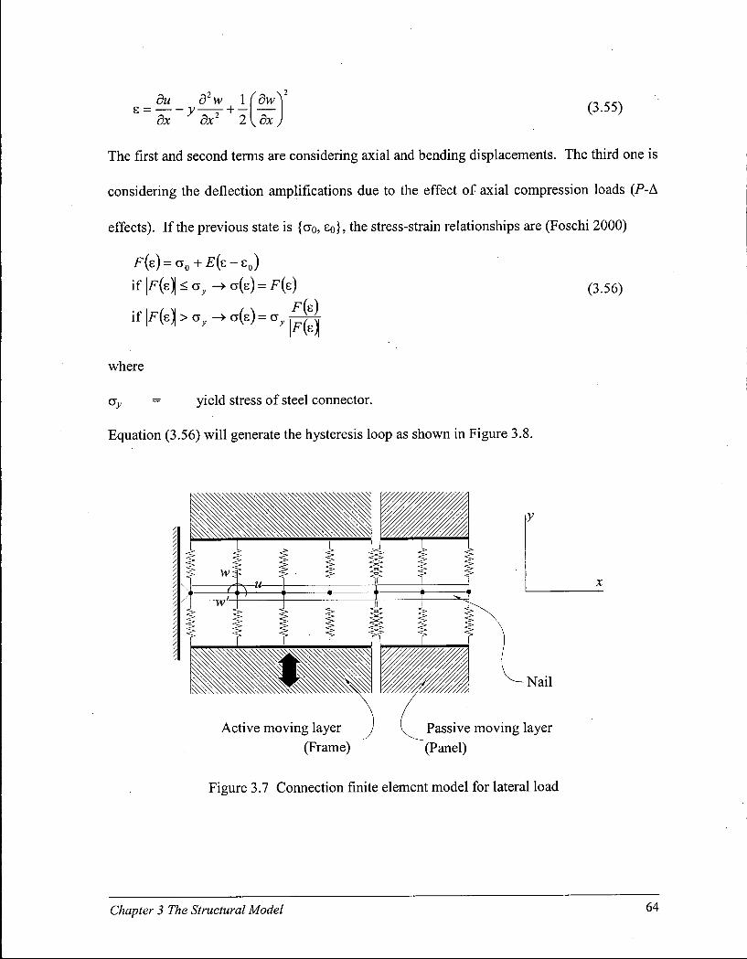
du d w 1 (dw s = y—r + - — dx dx 21 dx
\ 2
(3.55)
The first and second terms are considering axial and bending displacements. The third one is
considering the deflection amplifications due to the effect of axial compression loads (P-A
effects). If the previous state is {ao, So}, the stress-strain relationships are (Foschi 2000)
F(e) = o-0 + F ( s - s 0 )
i f |F (e^<a r ->a ( s )=F(s ) (3.56)
i f |F(e) > <jy -> a(e) = a}
Ffc)
where
= yield stress of steel connector.
Equation (3.56) will generate the hysteresis loop as shown in Figure 3.8.
Active moving layer (Frame)
Passive moving layer (Panel)
Figure 3.7 Connection finite element model for lateral load
Chapter 3 The Structural Model 64

a
Figure 3.8 Nail connector stress-strain relationship
The connector (nail) can be defined as a group of two-node beam elements acting on
a nonlinear foundation with linear axial and cubic bending deformation fields. The degree-
of-freedom vector is
a c = w,, vv,, dw, dx •,u2,w2,
dw2^ dx
(3.57)
The displacements represented by shape functions and degrees of freedom are
u = Ncmux + NCQ2u2 = N j c a c
w = M C 0 , w , +MC02
v d x J + MC03w2 +MC04
(dw,^
V d x )
= M j c a c
(3.58)
(3.59)
where
Ncoi, Mcoi shape functions for connection elements.
N o c , M o c = shape function vectors for connection elements.
The shape functions, after considering Jacobian transformations, are
7 V C 0 , =0.5-0.55
NC02 =0.5 + 0.5$
MC0l =0.5-0.75S+ 0.25f
Chapter 3 The Structural Model 65
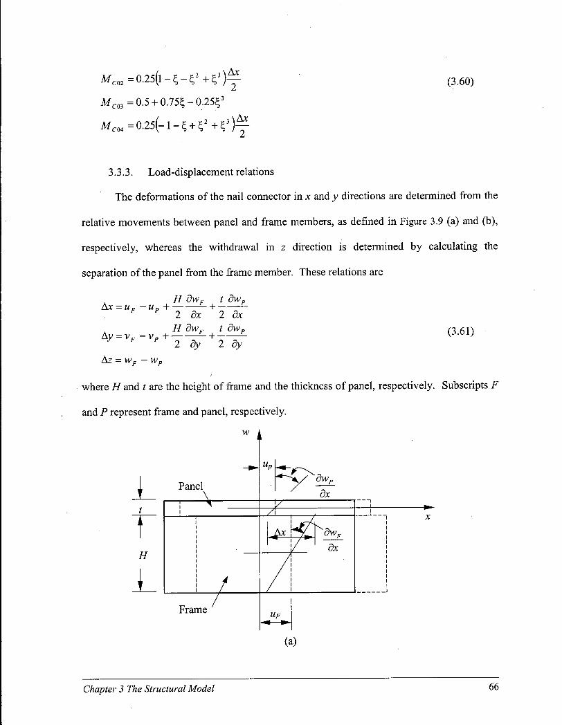
M C O 2 =0 .25 ( l -4 -4 2 +^ 3 ) Ax
(3.60)
MC03 =0.5 + 0.754 -0.254 3
M C O 4 = 0 . 2 5 ( - l - 4 + 4 2 + ^ 3 ) Ax
3.3.3. Load-displacement relations
The deformations of the nail connector in x and y directions are determined from the
relative movements between panel and frame members, as defined in Figure 3.9 (a) and (b),
respectively, whereas the withdrawal in z direction is determined by calculating the
separation of the panel from the frame member. These relations are
H dwF t dwp Ax = uF - up H h
Ay = vF-vp +
Az - wF -wp
2 dx 2 dx H dwP t dwp
+ • (3.61) 2 dy 2 dy
where H and t are the height of frame and the thickness of panel, respectively. Subscripts F
and P represent frame and panel, respectively.
H
Frame
(a)
Chapter 3 The Structural Model 66
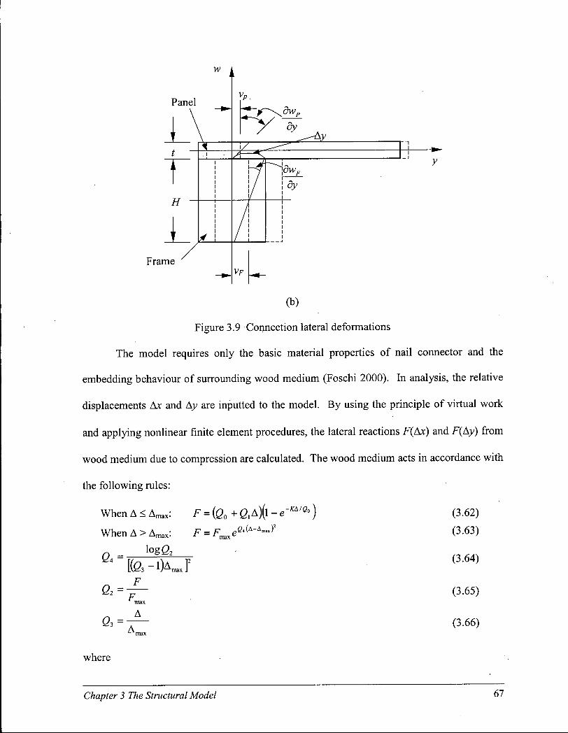
Frame
(b)
Figure 3.9 Connection lateral deformations
The model requires only the basic material properties of nail connector and the
embedding behaviour of surrounding wood medium (Foschi 2000). In analysis, the relative
displacements Ax and Ay are inputted to the model. By using the principle of virtual work
and applying nonlinear finite element procedures, the lateral reactions F(Ax) and F(Ay) from
wood medium due to compression are calculated. The wood medium acts in accordance with
the following rules:
When A < A m a x : F = (Q0 + Qx A)(l - <T* A / e°)
When A > AmaX: F = Fm„ e
0-2 =
log0 2
F F
max
A
(3.62)
(3.63)
(3.64)
(3.65)
(3.66)
where
Chapter 3 The Structural Model 67

F = resultant reaction force.
Qo = intercept of the asymptote.
Qi - asymptotic stiffness.
K = initial stiffness.
A = displacement.
Fmax = maximum resultant reaction force.
Amax = displacement at F m a x .
Assume that the previous state is given by force F at point b associating with
displacement A, in a loading or reloading. If the current displacement is greater than A, the
force will be decided by the rules shown in (3.62) and (3.63). Otherwise, the force is zero
until the displacement reaches the point a, after which the load-displacement relationship
follows the path a-b with a slope of the initial stiffness to meet the curve. In the course of
unloading, the wood medium recovers slightly from the nail compression so that the load-
displacement relationship follows the path b-a. When the fastener does not touch the wood,
the force is zero until it reaches the wood material on the opposite side.
The nail withdrawal force or panel-frame contact force F(Az) can be calculated
following a load-displacement relationship as shown in Figure 3.10(b). The same rules in
(3.62) and (3.63) apply. When panel separates from frame (nail withdrawal), i f Az in the
current step is greater than that in the previous step, the nail withdrawal load-displacement
relationship follows the curve o-c-b. Otherwise, it follows the path o-a-b, in which the
stiffness K\ is assumed to be a small proportion of the initial stiffness K. When the panel
touches the frame, the contact force is approximated as a linear function of the initial
stiffness K.
Chapter 3 The Structural Model 68

F(A) F(Az)
Az
A, 'max A=03A, 'max
(a) lateral deformation (b) withdrawal
Figure 3.10 Connection load-displacement relationships
3.4. The requirements of conforming elements
The use of conforming elements in the finite element analysis is necessary to achieve
a monotonic convergence, which means that the strain energy calculated by the finite element
solution converges to the exact strain energy of the mathematical model as the finite element
mesh is refined (Bathe 1996). When an element satisfies both completeness and
compatibility conditions, it is called a conforming element. The completeness requires that
the shape functions of the element must be able to represent the rigid body displacements and
the constant strain states. The compatibility requires that the displacements within the
elements and across the element boundaries are continuous, meaning no gap occurs between
elements when they are loaded. For elements with displacements, rotations, and twist
degrees of freedom, the continuity should be preserved to the second displacement
derivatives. By using the shape functions as described in the previous sections, the three
types of elements used in the model satisfy the requirements of completeness and
compatibility and, therefore, are assured to be conforming elements.
Chapter 3 The Structural Model 69

CHAPTER 4
FORMULATION OF STATIC NONLINEAR FINITE ELEMENT EQUATIONS
The finite element method was originally developed to analyze structural mechanics
problems and was then broadly applied to continuum problems and many other areas. The
method, as a numerical procedure, is very effective for problems unable to be solved
satisfactorily by classical theoretical methods. Instead of solving the differential equations of
equilibrium, the finite element method provides an approximate solution to variational
problems by minimizing a functional. In structural mechanics problems, a functional is the
expression for strain energy. In the current study, the principle of virtual work is adopted as
the basis of the nonlinear finite element formulation.
4.1. Principle of virtual work
In the case of a particle subjected to a system of forces, the principle of virtual work
states that i f the particle is in equilibrium, the total work of all forces acting on the particle in
any virtual displacement is zero (Timoshenko 1970). If 5w, 8v and bw are components of a
virtual displacement in the x, y, and z directions, and 1,RX, l,Ry and zZRz are the sums of
projections of forces acting on the particle in the same directions, the principle of virtual
work gives
bWx = bu^Rx =0 bWy = bvJ^Ry =0 bWz = 6 w £ i ? z = 0 (4.1)
Chapter 4 Formulation of Static Nonlinear Finite Element Equations 70

The equations are satisfied for any virtual displacement i f
IX=o 5x=° i x =o (4.2)
Consider a general three-dimensional body as shown in Figure 4.1. The body is
subject to concentrated forces rc, surface tractions r^, and body forces rB. These forces
represent all externally applied forces and reactions in three-dimensional space. The
principle of virtual work, when applied to the body, states that equilibrium of the body
requires that for any compatible small virtual displacements imposed onto the body, the total
internal work is equal to the total external work.
kz,w
Figure 4.1 General three-dimension body
The principle can be expressed as
hW = bWj +bWE = 0 (4.3)
where the internal work is
hW, = jobedV (4.4) v
and the external work is
Chapter 4 Formulation of Static Nonlinear Finite Element Equations 71

8 ^ = - ( R B + R 5 + R c ) S a = - J i rBdudV - jrs5udA - ^ r c 8 a (4.5) V A
In these equations, 8u is an arbitrary virtual displacement field, Se is the
corresponding virtual strain vector, and 8a is the nodal degree of freedom vector. The vector
8u satisfies the boundary conditions of the problem and can be expressed as a linear
combination of shape functions and nodal degrees of freedom. R c is a vector of the
externally applied concentrated forces rc to the nodes of the element assemblage. The z'th
component in Rc corresponds to the z'th degree of freedom in a. R B and Rs represent the
vectors of body forces r# and externally applied surface forces (usually distributed loads) r^.
It is noted that the body forces due to gravity in Equation (4.5) may be considered as less
important than the surface forces r$ in statically loaded structures. Therefore, they are
excluded in the static finite element analysis. In dynamically loaded structures, inertia forces
are generated from the body forces and need to be integrated into the dynamic finite element
analysis (Chapter 6).
4.2. Internal virtual work in elements
4.2.1. Internal virtual work in plate element
The constitutive relationships for a plate element in Equation (3.13) can be expressed
as follows
0
0 1 - V V
xy yx 1 — V V
xy
0 0 G xy (4.6)
Chapter 4 Formulation of Static Nonlinear Finite Element Equations 72

Ex , VxyEx Zx + E y
1 — v v 1 — v v xy yx xy yx
l - v„ ,v . „ 1-v v xy yx
G y xy i xy
Substituting Equation (4.6) into Equation (4.4) yields the internal virtual work of the plate
element
V ^ xyN yx
+ f — [v e 8s + 8 8s \lV J l _ v v x
V xy yx
+ iGxyJxy^xydV
(4.7)
Using the strain-displacement relationships developed in Chapter 3, Equation (4.7) can be
expressed in terms of shape functions and natural coordinates.
( « r , ) , - # £ Sa
+ 8aT
+ 8aT
+ 8aT
+ 5aT
+ 8aT
2 2 I L r /
11° M J M * + ± M J V 1 * N I J ( » dtfh\
-M^M^a + L, ,
JJ[ZJ v(L,X + N , X > * V ( M 2 , M L + M 2 , M ^ ) k * l .51
.51
Jj£>v i a T ( M u M ; j t M , X , +M„M?yM1X,)>
+ ±(MlxMlLly + M , X N , ) a + a T ( N 1 I M , M ^ L l y M 1 X ) d$dr\
(4.8)
Chapter 4 Formulation of Static Nonlinear Finite Element Equations 73
+ 8aT
+ 8aT
J j [ D c ( N l y + L , J N „ + L , J T + 4 * C M 2 V M ^ ] * i r f n
.5 n
where
and
EX, Ey
G xy
+
J J / ) c [ a T ( N l y + L L J T + M U M ^ » X M u M ' , + M>X,)
5 n
1 - v v yx
D., =• 1 — V V
A. = v E t v E t
y j r y . \ r _ * yx^y* l -v„,v„, 1-v v.
Do
Ky
K.. =•
Et 1 2 ( l - % v y , )
Eyf 1 2 ( 1-v^)
VxyE/ v E r yx y 12(l-v v ) 1 2 ( l - v , ^ t )
Kr=Gr
12
(4.9)
(4.10)
(4.11)
(4.12)
(4.13)
(4.14)
(4.15)
(4.16)
= Young's modulus in x and y directions, respectively.
= shear modulus.
= Poisson's ratios.
t = thickness of panel elements.
A l l of the definitions of shape functions can be found in Equations (3.36)-(3.44) in
Chapter 3.
The above internal virtual work expression includes the work done by the elongation
and bending of the middle plane of the plate and the work done by the large deflection due to
Chapter 4 Formulation of Static Nonlinear Finite Element Equations 74
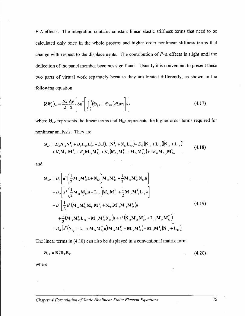
P-A effects. The integration contains constant linear elastic stiffness terms that need to be
calculated only once in the whole process and higher order nonlinear stiffness terms that
change with respect to the displacements. The contribution of P-A effects is slight until the
deflection of the panel member becomes significant. Usually it is convenient to present these
two parts of virtual work separately because they are treated differently, as shown in the
following equation
4 n
(4.17)
where QLP represents the linear terms and QNP represents the higher order terms required for
nonlinear analysis. They are
+ KxM2xMT
2x +KyMlyMly +Kv(M2yMT
2x +M2,MjJ+4*cM2jg,M̂ (4.18)
and
+ D, J\y J"M\y1,M-iy ' 2 '.v '.v
+ A I T
+
aT(MuM* M.X, +MI>MT,M1JlMT,)a
+ i(M,,M7cLly +MlrMT,N,,)a + aT(NuMlyM; + L1,M,,MT,)
/)c[aT(Nly +LU + MUMT
>»XM.X, +MlyM[J+MuM (̂N., + L>J
The linear terms in (4.18) can also be displayed in a conventional matrix form
(4.19)
(4.20)
where
Chapter 4 Formulation of Static Nonlinear Finite Element Equations 75
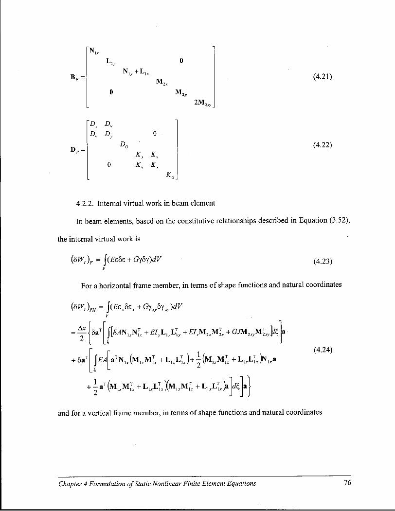
N ,
N L Y + L U
M ,
M 2y 2M 2.xy
(4.21)
D„ D„ (4.22)
4.2.2. Internal virtual work in beam element
In beam elements, based on the constitutive relationships described in Equation (3.52),
the internal virtual work is
(&Wr)F = J (£eSs + Gy&y)dV ( 4 2 3 )
V
For a horizontal frame member, in terms of shape functions and natural coordinates
(S^,L = S(Esxtex+GyxySyxy)dV V
5aT J [ ^ N l x N L + EIyLiyh]y + EIM2xMT
2x + GJM2xyMr
2xy]^ .4
+ 5a T | j £ ^ a T N 1 I ( M , X , + L . x L L ) + + ^ > , , a
A x
~2~ (4.24)
i a T (M 1 X M* + L , X X M , ^ + L , X y
and for a vertical frame member, in terms of shape functions and natural coordinates
Chapter 4 Formulation of Static Nonlinear Finite Element Equations 76
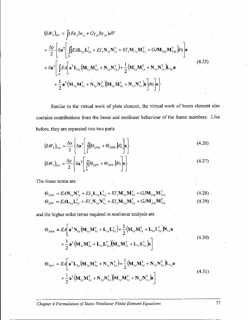
5a 1
{W,)Fv = j ( ^ X + Gyyx5yyx)dV
J [ f i 4 L , X +EIXN,XX + EI 2M2yMr
2y +GM2vMT
2xy}h\ .n
{£/l[a TL l y(M l rM^ + N , X ) + j ( M . X , + N X K a
= 4? 2
+ 5a T
(4.25)
+ i aT (M„M£- + N,^N^ K X + N , X V
Similar to the virtual work of plate element, the virtual work of beam element also
contains contributions from the linear and nonlinear behaviour of the frame members. Like
before, they are separated into two parts
(8*",} Ax FH
5a 1
8a 1
J[®LFH+®NFHH
The linear terms are
® L F H = £ 4 N , X + EIyLlyL]y +EI2M2xMT
2x +GJM2xyM
@LFr=EAhu,Ll,+EIrNw^l+EIM7M,+GJM2xvMl
T 2xy
'\y^ly ^^x^lx^Xx ^ ^ z'^ly'^ly 2xy1J*2xy
and the higher order terms required in nonlinear analysis are
®NFH = EA a T N u H X +Llxh]x)+\(M}xMl + L I I L j > I , a
®NFy = EA\
+ l a T ( M X + N , X K M i + N . X ) a
(4.26)
(4.27)
(4.28)
(4.29)
(4.30)
(4.31)
Chapter 4 Formulation of Static Nonlinear Finite Element Equations 11
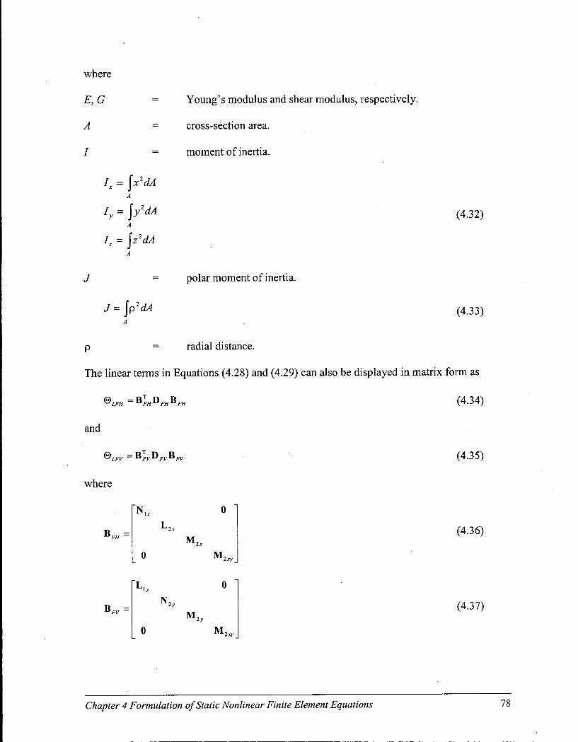
where
E, G
A
I
Young's modulus and shear modulus, respectively,
cross-section area,
moment of inertia.
Ix = \x2dA A
iy = \y2dA A
Iz = \z2dA
(4.32)
J polar moment of inertia.
J=jp2dA (4.33)
p = radial distance.
The linear terms in Equations (4.28) and (4.29) can also be displayed in matrix form as
(4.34) ®LFH — ^FH^FH^FH
and
®LFV ~ ^FV^FV^FV (4.35)
where
B,
N,
M ,
M 2*y
(4.36)
N 2 y
M 2y M 2*y.
(4.37)
Chapter 4 Formulation of Static Nonlinear Finite Element Equations

EA 0 EI,
ET. 0 G J
' £ 4 0 "
Eh ET.
0 GJ
(4.38)
(4.39)
4.2.3. Internal virtual work in connection element
From Equation (3.61), the virtual deformations of a connection element represented
by the shape functions are
8Ax = (NJ„ - N 0
T + ^M* )sa = Q>
8Az = ( M j f - M j ) 5 a = Qj8a
Where the Q's are the shape function combinations.
External virtual work done by a connection element in three directions is
(5 WE)C=YJI" ^(Ax)8Ax - F(Ay)8Ay - F(Az)8Az]
Since
(s^)c + (srJc = o Therefore, the equivalent internal virtual work in a connection element is
(8W, ) c = £ [^(Ax)SAx + F(Aj/)8A.y + F(Az)SAz]
= X [ F ( A x ) Q > + F ( A y ) Q > + F(Az)Qj8a]
(4.40)
(4.41)
(4.42)
(4.43)
(4.44)
(4.45)
Chapter 4 Formulation of Static Nonlinear Finite Element Equations 79

4.3. Formulation of external force vector
Under static loading conditions, the structure to be analyzed is subject to in-plane
concentrated loads, out-of-plane uniformly distributed loads, or a combination of both. The
concentrated loads in the model are required to be assigned to the nodes of the frame
elements, whereas the uniformly distributed loads need to be assigned on the surface of the
exterior panels (normal to the surface). These loads represent the weights of the structural
components (vertical constant load), the weights of snow and rain (vertical live loads), and
the lateral live loads. The lateral loads are applied to structure for the purpose of simulating
the action of wind and earthquake. The loading rate is very low to avoid any possible
influence due to severe variation of material strain rate. Although this type of loading is
usually referred to "quasi-static" loading and is associated with cyclic tests, the unidirectional
monotonic loading is often used in the studies of lateral resistance of structures.
The concentrated load vector can be formed by simply accounting all of the external
concentrated loads, which is
Referring to the illustration in Figure 4.2 a consistent load vector for the uniformly
distributed loads can be derived. Assume a uniformly distributed load q(x, y) to be acting on
a patch of a panel element. From the expression of the external virtual work by surface
forces in Equation (4.5), the virtual work by distributed loads is
(4.46)
A A
J J q ( * ^ ) ^ ' ^ ' M „ f e W ) 8 : (4.47)
a
Based on the geometry in Figure 4.2, the following relations can be found
Chapter 4 Formulation of Static Nonlinear Finite Element Equations 80
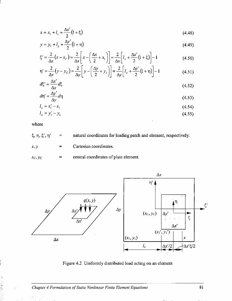
S' = — (x-j:c) = — I; Ax Ax
i ' = — ( y - y c ) = — I Ay Ay
Ax' Ax
Av lx= xx — X ,
' r = y,' - y,
Ax + x,
Av + y,
_2_ Ax
_2_ = A^
• l
- l
where
*,y
*c,.yc
(4.48)
(4.49)
(4.50)
(4.51)
(4.52)
(4.53)
(4.54)
(4.55)
natural coordinates for loading patch and element, respectively.
Cartesian coordinates.
central coordinates of plate element.
Figure 4.2 Uniformly distributed load acting on an element
Chapter 4 Formulation of Static Nonlinear Finite Element Equations 81

Substituting the relations in (4.52) and (4.53) into (4.47), and applying relations (4.50) and
(4.51) to the shape functions Mo, result in the following,
( 5 ^ ) , - - J J q ( ^ ^ ^ ^ ^ ^ M 0 ( 5 , r 1 ) 5 a ( 4 5 6 )
The consistent load vector for uniformly distributed surface forces is
R 5 = lfa(x,y)^d^dr\M0{c,,r]) (4 57)
k n
4.4. Formulation and solution of system equations
The principle of virtual work can be now applied to the whole system to formulate the
equations at element level required for the solution. The element tangent stiffness is
calculated first and then assembled into a global stiffness matrix using standard finite
element procedures. During the assembling, a three-dimensional transformation is required
to ensure that all the elements are in a common global coordinate system (Chapter 5). The
global stiffness matrix is then solved by a numerical integration method, Gauss quadrature,
which is carried out at each Gauss point for the whole system. The global solution vector a,+i
is computed by a selected iteration scheme with appropriate boundary conditions imposed.
From the previously introduced expressions for panel element, frame elements, connection
elements, and the externally applied forces, the total virtual work in an element under static
state is
(hW\ +(5W,)FH +(bWl)py +(5W\-(5WE)S - R c 5 a = 0 (4.58)
Differentiating Equation (4.58) with respect to 8a, an element out-of-balance load
vector \\ie can be obtained
Chapter 4 Formulation of Static Nonlinear Finite Element Equations 82
We Ax Ay ~2~~2~ 4 n
Ax a +
Ay j[&LFV +®NFV}ir} (4.59)
+ £[F(Ax )Ql + F(Ay)Q] + F(Az)Q] ]-Rs - Rc = 0
or
vi/e = f - R , - R c = 0 (4.60)
where
f = the force containing contributions from the linear and nonlinear
behaviour of panel and frame members, and from the nonlinear behaviour of nail
connections. It is
~ _ Ax Ay 2 2
4 Tl
Ax ~1 a +
Ay (4.61)
+
.1
X [F(Ax)Q] + F(Ay)Q] + F(Az)Q]}
The vector \j / e is obtained first for each element and then assembled into the
corresponding global out-of-balance load vector T. The vector ¥ can be interpreted as the
difference between the resisting forces of the structure and the externally applied loads.
When this difference is zero, the whole structure is in equilibrium and the unknown nodal
point variables will converge to a set of new values corresponding to the preset displacement
or load conditions. Since the resisting forces are not single valued but depend nonlinearly on
the nodal point displacements, an iterative procedure is needed to find the solutions of the
equations T to satisfy the finite element equilibrium requirements.
Chapter 4 Formulation of Static Nonlinear Finite Element Equations 83
One of most frequently used iterative schemes for the nonlinear finite element
equations, the Newton-Raphson method, is implemented in the algorithm. This solution
method involves repeat calculations of increments in the nodal point displacement, which
defines a new displacement vector, until the out-of-balance load vector *F to be zero. The
currently used Newton-Raphson method usually leads the solution,to a rapid convergence
within a few iterations when the absolute values of the tangent stiffness are large. However,
the convergence by this method is not guaranteed when the tangent stiffness value is close to
zero (the flattening parts of the load-displacement curve). In this situation, the solution may
converge very slowly or, sometimes, may divergence. To ensure a convergence, some self-
adaptive procedures are implemented into the program, as described in Section 4.7.3. An
alternative presentation of Newton-Raphson is the modified Newton-Raphson, which differs
from the Newton-Raphson only in that the tangent stiffness matrix is not updated during
iterations within one step. The benefit of using the modified Newton-Raphson is that the
expensive repetitions of forming and reducing the tangent stiffness matrix can be avoided.
However, the study found (Cook 1989, Ch. 17) that the modified Newton-Raphson method
did not perform well when the load-displacement curve displays a hardening or pinching
behaviour. In this situation, the iterations are more likely to converge slowly or fail to
converge.
The general equations used in the Newton-Raphson iteration (illustrated in Figure
4.3), for i'=l, 2, 3, are:
K.Aa,. = - ¥ , . (4.62)
a,+1 = a,. + Aa,. ; (4.63)
In these equations, the loads are assumed to be independent of the deformations. The
Chapter 4 Formulation of Static Nonlinear Finite Element Equations 84

initial conditions are ai, Ko, and Pa.
Slope Ko Slope K i Slope K 2
ai a 2 a 3 ... a„ a
Figure 4.3 Newton-Raphson iteration starting from point a and converging at point b
If the displacement vector a, is evaluated in the iterative solution, a Taylor series
expansion of the vector truncated after the first derivative, is
VM = f f +^-Aa, . = ¥ , +AT(a, + 1 -a , ) 3a
where the subscript i represents the z'th iteration.
The component
(4.64)
3a (4.65)
is the global tangent stiffness matrix, which is the assemblage of element tangent stiffness
matrices at the ith iteration.
Assuming that the out-of-balance load vector is zero in the 0'+l)fh iteration, an
updated displacement vector a J + i can be obtained from Equation (4.64) based on the vectors
and a, from the current iteration
a , ,=a ,+ (Ay )-•(-*,) (4.66)
Chapter 4 Formulation of Static Nonlinear Finite Element Equations 85
An element tangent stiffness matrix is obtained by differentiating the equation (4.59)
d\\ie _ Ax Ay
+ •
+
Ax + Ay
\(®LFV +®NFv)dri
dF(Ax)QT ( dF(Ay)QT | dF(Az) q T
SAx " A SA^ 5Az
4 n
(4.67)
+
+
y 1 j 0 ^ ^ + y j©*™^+4r I®,™** 4 1
5 F ( A x ) Q T | dF(Ay) q T ; dF(Az) q T
d Ax ~* dAy
= (k)L+(k)N=kT
dAz
where
k r = element tangent stiffness matrix.
( k ) ^ = linear part of element tangent stiffness matrix, which is constant and
calculated only once.
(k)yv = nonlinear part of element tangent stiffness matrix, which is updated for
each step.
Accordingly, the global stiffness matrix can be expressed as
da
where
(K)i
= K, = = Eto*+Xto* = (K)̂ +(K)*
= global tangent stiffness matrix.
= linear part of global tangent stiffness matrix.
= nonlinear part of global tangent stiffness matrix.
(4.68)
Chapter 4 Formulation of Static Nonlinear Finite Element Equations 86

The integrals in the tangent stiffness matrix presented in equation (4.67) have to be
evaluated numerically and updated at each step. The Gauss quadrature has been proven the
most useful quadrature rule in numerical integration and is implemented in the
LightFrame3D program.
One- and two-dimensional integrals can be expressed approximately as polynomials,
as shown respectively in the following equations.
J/tete=Z^,/fo) ( 4 - 6 9 )
JJ / f e n ^ r , = J l W i l y ) (4-7°) - i - i i i
where
n = order of numerical integration or number of Gauss points.
Wi, Wj = weighting factors.
/ ( £ , ) and fl^i,y]j) are /(^) and f{t,,v\) evaluated at the Gauss points, respectively.
The determination of the number of Gauss points is based on the orders of / (^) and
/(4,r|). Generally, the n Gauss points are needed to evaluate those matrices exactly up to
the order of (2M-1). In the nonlinear finite element analysis, however, the determination of
the number of Gauss points is not as simple, due to the difficulty in examining the order of
the nonlinear potion of the stiffness matrix. Although the number of Gauss points can be
decided by changing them in the program and comparing the errors in results, it is believed
that a satisfactory accuracy is achieved by selecting the number of Gauss points just
according to the order of the linear potion of the stiffness matrix, since the influence from the
much higher orders on the results is negligible. The final choice of the number of Gauss
Chapter 4 Formulation of Static Nonlinear Finite Element Equations 87

points should also consider the balance between the accuracy and the cost of the analysis.
Using more Gauss points to achieve slightly improved accuracy of the results may not be
practical in the analysis, especially in three-dimensional analysis, because the cost can
increase significantly.
From the equations (4.18), (4.28) or (4.29) by referring to the Pascal triangle, the
highest order of the linear potion of the stiffness matrices is determined to be six, as shown in
equation (4.71). The required number of Gauss points is four, which can evaluate the
stiffness matrix exactly up to the order of seven.
/ = / f e 6 , W ^ V , § 2 T l 6 , T l 6 ) (4-71)
The sampling points and weighting factors for four Gauss point integration are listed in
double-precision as follows:
or Vj Wt or Wj
±0.86113 63115 94053 0.34785 48451 37454
±0.33998 10435 84856 0.65214 51548 62546
4.5. Element stress calculations
After element stiffness matrices are assembled into the global stiffness matrix and the
nodal point displacement vector is solved using the Newton-Raphson iterative procedure, the
element stresses are calculated in the post-processor, the final phase of the analysis.
4.5.1. Panel stresses and central deflection
Recall the expressions of panel normal and shear strains derived in Chapter 3
, „ du \ s* =e' +e" = — + —
x x x dx 2
1dw^ -z^ (4.72) dx2
Chapter 4 Formulation of Static Nonlinear Finite Element Equations 88

dv 1 dy + 2
du dv dw dw
8 = 8 + 8 = h y y y dy 2
y = — + h-I xy
dw
\fy J
-2z
- z-d2w dy2
d2w
(4.73)
(4.74) xy dy dx dx dy dxdy
Using the first and second derivatives of shape functions (Equations 3.36 - 3.44 in Chapter
3) to represent these strains gives
The normal and shear stresses in panel are obtained as
(4.75)
(4.76)
(4.77)
£, = D
y y T "f xy _
(4.78)
where
D =
VxyEx
1 — V V xy yx
v E yx y
1 — V V xy yx
1—V V 1 — V V xy yx xy yx
0 0
0
0 (4.79)
The deflection at the center of a plate element is .calculated by using the relationship
when the natural coordinates £, and n are taken to be zero
w = MT
0a (4.80)
4.5.2. Frame bending stress
The normal strains in a horizontal and vertical beam element are, respectively
Chapter 4 Formulation of Static Nonlinear Finite Element Equations 89

du 1 (dw zx = — + - —
dx 2\ dx Y 1
+— J 2 [dxj
d2w d2v •z—- - y—T . dx2 dx2
(4.81)
dv 1 fdw} +•
d2w d2u - Z r~x T
dy2 dy2
When expressed by the derivatives of shape functions, the strains are
e, = N?> +1 a ' M . M ^ a + i a T L u L ^ a - zM^a - vLT
2 j (a
Then the stresses in a horizontal and vertical beam element are, respectively
(4.82)
(4.83)
(4.84)
(4.85)
4.6. Displacement control method
Displacement and load controls are two options that can be selected as input history
in the static finite element analysis by using the LightFrame3D_Static program. In
displacement control, the incremental displacement is used as stepping parameter, and in load
control, the incremental load as stepping parameter. In terms of the program coding, both
methods do not show much difference; however, in practical applications, the selection of the
control method should be based on the problems to be studied and the results sought because
the two methods do give different outputs. The displacement control method allows the
analysis to go beyond the maximum capacity of the system to provide a complete load-
displacement path. Usually it is desirable that the analysis could predict the entire
deformation history including the post-peak behaviour of the structure. It is also useful when
the analytical results are compared with the testing backbone curves. Load control method
can not satisfy this requirement because the stiffness matrix wil l be ill-conditioned at the
Chapter 4 Formulation of Static Nonlinear Finite Element Equations 90
maximum load level. The displacement control method can be easily used to follow
multiple loading-unloading-reloading paths as in a cyclic procedure, in which groups of
cycles with prescribed displacement amplitudes are applied to the structure to study the
stiffness and strength degradations and the pitching effects. The load control method,
however, is difficult to be used for this purpose.
The only difference between the displacement control and load control is that an
incremental displacement step is assigned to the designated degree of freedom in the
displacement vector a before solving the system equations, and the convergence is checked
by using the criterion (4.88) to evaluate the resultant loads of subsequent iterations at that
degree of freedom. In Chapter 9, detailed descriptions are given for the predictions made by
the LighfFrame3D program using displacement control mode.
4.7. Convergence considerations
4.7.1. Convergence checking and criteria
In the nonlinear finite element analysis, convergence rate is strongly problem-
dependent. The convergence could be achieved very quickly, such as within two or three
iterations, when the structure is mainly in its linear elastic range, while the problem requires
more iteration to achieve convergence when the structure is approaching its maximum
capacity, at which the tangent stiffness is close to zero. Sometimes, divergence may occur
due to the physical instability of the structure. In such cases, the structure can be typically
defined as failed. To ensure convergence at each step, convergence-enhancement features
were implemented into LightFrame3D programs to activate the self-adaptive procedures i f
the solution does not converge after required number of iterations (see Section 4.7.3). In all
the iterative processes of the current nonlinear finite element analysis, the solutions are only
Chapter 4 Formulation of Static Nonlinear Finite Element Equations 91
approximately achieved and some tolerance limits have to be set to terminate the iteration.
The selection of tolerances should be realistic. If the convergence tolerances are top liberal,
the solution is inaccurate and error can accumulate to cause difficulties for the later steps to
converge. If the tolerances are too tight, either the highly accurate solution cannot be
obtained or much computational effort is spent to obtain unnecessary accuracy.
The following convergence criteria are used in the nonlinear finite element programs.
Criterion 1.
l l A a / | | y y - £ " ( 4 - 8 6 ) F i l l
This criterion requires that the norm of the displacements at the end of iteration be
within a certain tolerance of the true displacement solution. This criterion is used when
the problem is under the load control mode in a static analysis.
Criterion 2.
M < e j Y j (4.87)
This criterion requires that the norm of the out-of-balance load vector at the end of an
iteration be within a certain tolerance zF of the initial load increment. In the application of
this criterion, a few problems were noticed. The variation in the magnitude of the initial load
increment *Fi may cause the change in convergence rate for different steps. In the case of
small initial load increment, the convergence in the out-of-balance load may not imply the
convergence in the displacements. In addition, the out-of-balance load vector contains
quantities in different units. Due to these problems, this criterion is only used for
displacement control mode in a static analysis. Considering that the whole structure is in
equilibrium under static loading, Equation (4.87) can be simplified to compare the load value
Chapter 4 Formulation of Static Nonlinear Finite Element Equations 92

at the nodal point where the specified displacements are applied. The criterion becomes
K-P^zF\Pi\ (4.88)
4.7.2. Ill-conditioned stiffness matrix
In nonlinear finite element analysis, the tangent stiffness matrix may become i l l -
conditioned i f there is a significant difference in the values of the stiffness coefficients.
Under such circumstances, the solution vector (usually nodal displacement vector) can be
sensitive to small changes in the stiffness matrix and thus lead to erroneous results. The
diagonal coefficients of the matrix can also be zero- or near zero-valued due to the truncation
errors, even i f double precision is used. There are several reasons for the ill-conditioned
stiffness matrix. First, ill-conditioning may reflect the physical reality of a structure with low
tangent stiffness because it is near failure or collapse. For example, under the load control
mode, when the structure reaches its maximum capacity, the occurrence of ill-conditioned
stiffness matrix implies that the analysis should be terminated. Second, ill-conditioning may
arise when the elements in the problem become physically unstable. In the mechanics-based
nail model in the finite element program, when the gaps between the nail elements and the
wood medium are formed, the nail connector can have virtually zero stiffness because the
wood medium only acts in compression. This physical instability in nail connections during
deformation is believed to be a reason resulting in the ill-conditioned stiffness matrix. Third,
ill-conditioning may occur i f the stiffness between the contacted elements is very high but
there is no room for them to deform. This problem was detected when the panel-frame
contact model in the program was developed. A correctly defined relationship between
contact stiffness and deformation can effectively prevent the ill-conditioning from occurring.
Finally, the mixing elements in the finite element model may be another reason to induce i l l -
Chapter 4 Formulation of Static Nonlinear Finite Element Equations 93

conditioning.
The stiffness matrix is checked for ill-conditioning before the solution procedure of
the equilibrium equations starts. In the solution procedure, a decomposition method,
Cholesky factorization in the current finite element model, requires that a stiffness matrix has
to be positive definite. In case the ill-conditioned stiffness matrix occurs, the second self-
adaptive procedure (Section 4.7.3) will initiate.
4.7.3. Self-adaptive procedures
The following four self-adaptive procedures are implemented in the program
algorithms:
Procedure 1. During the analysis, the norm of solution possibly does not converge to the
preset tolerance after a large number of iterations because some of the dominant
displacements swing from one point to another alternatively. Figure 4.4 illustrates an
example occurring in the iteration procedure in which the searching repeatedly goes between
a3 and a 4 while the convergence is never achieved.
P
Aa3
ai a4 a2 a3 a
Figure 4.4 Cyclical searching in the Newton-Raphson iteration method
Chapter 4 Formulation of Static Nonlinear Finite Element Equations 94
In this situation, the procedure will update the unknown displacement vector by
adding one-half of displacement increments from the current iteration to the next, as shown
in (4.89)
a, = a M +0.5Aa. (4.89)
This procedure is applicable to both load and displacement control modes and can
effectively improve the solution mechanism. Usually, convergence can then be achieved
rapidly.
Procedure 2. If the solution cannot satisfy the convergence requirements after the preset
number of iterations or i f the stiffness matrix is ill-conditioned, the simulation of the current
step will restart with the step size being halved. Usually, repeating the procedure once or
twice wil l lead to a converged solution.
Procedure 3. Procedure 2 sometimes may not be very effective to solve the convergence
problem because the structure could be in a physically unstable state. For example, when a
nail is situated in a large hole, further reduction in step size does not solve the convergence
problem. In this case, an increase in step size is needed to allow the nail to engage the wood
medium again in reaching a new stable state. Therefore, i f the solution does not converge
after the preset number of reduction in the step dimension, the current step is abandoned and
the program proceeds to the next step. In both procedures 2 and 3, the calculation needs to
restart from the last converged solution.
Procedure 4. In some cases, the norm of displacement vector or the norm of load vector is
found to be very close to the tolerances but not within it after a number of iterations. A slight
relaxation in the tolerances is given to let the step finish.
If all attempts from these procedures fail, the execution is terminated. This situation
Chapter 4 Formulation of Static Nonlinear Finite Element Equations 95
implies that either the structure reaches failure or the structural model is incorrect. In the
second case, the model should be carefully checked and appropriate modifications have to be
done to improve the analysis.
4.8. Further expansion of the program
The LighfFrame3D program requires the exterior or interior panels in a structural
model to have the same thickness and material properties. This limitation will not affect the
application of the program to the building components, in which usually only one type of
panels is used. In the building study, this limitation may cause some difficulties i f more than
one type of panels need to be used. Modification in the variables defining the panel
properties in the program can remove this limitation to allow the panels to have different
thickness, orientation, and material properties.
The displacement control of the program is designed to apply to one node of the
structural model. Although it is satisfactory in most light-frame building studies, an
expansion can be made to suit the requirement for a multiple-point displacement control.
Chapter 4 Formulation of Static Nonlinear Finite Element Equations 96
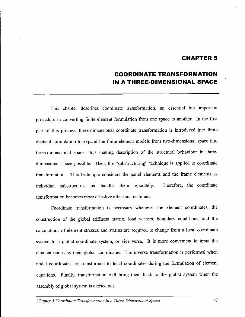
CHAPTER 5
COORDINATE TRANSFORMATION IN A THREE-DIMENSIONAL SPACE
This chapter describes coordinate transformation, an essential but important
procedure in converting finite element formulation from one space to another. In the first
part of this process, three-dimensional coordinate transformation is introduced into finite
element formulation to expand the finite element models from two-dimensional space into
three-dimensional space, thus making description of the structural behaviour in three-
dimensional space possible. Then, the "substructuring" technique is applied to coordinate
transformation. This technique considers the panel elements and the frame elements as
individual substructures and handles them separately. Therefore, the coordinate
transformation becomes more effective after this treatment.
Coordinate transformation is necessary whenever the element coordinates, the
construction of the global stiffness matrix, load vectors, boundary conditions, and the
calculations of element stresses and strains are required to change from a local coordinate
system to a global coordinate system, or vice versa. It is more convenient to input the
element nodes by their global coordinates. The inverse transformation is performed when
nodal coordinates are transformed to local coordinates during the formulation of element
equations. Finally, transformation will bring them back to the global system when the
assembly of global system is carried out.
Chapter 5 Coordinate Transformation in a Three-Dimensional Space 97
5.1. Coordinate transformation
Figure 5.1 shows an element arbitrarily located in three-dimensional space. Let {Xt,
Yi, Zi) represent global nodal coordinates, ( X . ^ Z , . ) local nodal coordinates, and X° , Y° ,
and Z° be identity vectors along the edges of the element in X, Y, and Z directions,
respectively.
A y
(X,, Y,, Zi)
0 Li i (Xo, Y0, Z0) (X,, Y,, Zi)
X
Figure 5.1 Coordinate transformation
The local nodal coordinates (Xi,Yi,Zi) can be expressed in terms of global nodal
coordinates (Xi, F„ Z ;) as
(5.1) = T
where the transformation matrix, T, can be established as follows
/. m, n
T = 12 m2 n2
13 m3 «3
/,-, nii, nt = direction cosines, i = 1, 2, 3.
Vectors X°and Y°can be expressed as
(5.2)
Chapter 5 Coordinate Transformation in a Three-Dimensional Space 98
X° = /,i + mx j + »,k = i - A i + j + Z ^ A k ( 5 .3)
A A A
Y° =/ 2 i + m 2j + » 2 k = X 2 ~ X o i + ̂ ^ j + Z 2 " Z ° k (5.4) A A A
where
L^^-Xj+fc-Yj+fr-Zj (5.5)
Z 2 = V(̂ 2 -X 0 ) 2 + (Y2 -Y0f+ (Z 2 - Zj (5.6)
i , j , k = unit vectors.
Vector Z° therefore is
Z° = X ° x Y° =/ 3 i + w 3 j + « 3 k (5.7)
where
(5.8) ! (Yi-Yofa-Zo) {Y2-YQ\Z,-Z0)
w = ( ^ 2 ~̂oX-̂ l ~̂o) (^l~^o)(^2~^o) ^ g)
{Xt-X0XY2-Y0) (X.-XjY.-Y,) 3 _ z z z z 1 ;
For a general case in which the angle 0 between X°and Y°is not 90° (non-rectangular
component), the direction cosines of Y axis needs to be recalculated to ensure that all three
axes X, Y , and Z are orthogonal
r = z°xx° (5. i i )
The transformation matrix needs to have the following three properties
(1) cos2(5,50=1 Yj(lm + mn + nl) = 0 (S = X,Y,Z) (5.12) i ( i
(2) |T| = ±1 ( 5 - 1 3 )
(3) T T = T - ] (5-14)
Chapter 5 Coordinate Transformation in a Three-Dimensional Space 99

5.2. Stiffness matrix transformation
In the process of transformation, when local element stiffness matrices are assembled
into a global stiffness matrix, "substructuring" is applied to avoid introducing unnecessary
higher order degrees of freedom, some of which will be meaningless after transformation.
The panel elements and frame elements can be considered as different substructures and can
be treated separately. This is possible because panels are connected to frame members by
nails only; there is no direct physical connection among panels themselves. By using the
substructuring technique, panel elements and frame elements, which are under different
coordinate systems, can be assembled into one global system, without increasing the
complexity of the analysis. The substructuring procedure used here is not the same as that in
a "superelement" procedure, in which a single element can have many boundary and interior
degrees of freedom with only boundary degrees of freedom connected to other outside
elements. In the substructures of panel elements and frame elements, however, all of the
degrees of freedom will be connected to each other via nail connectors. In the process, the
transformation of stiffness is only performed in frame elements, during which the stiffness
coefficients associating with three translational and three rotational degrees of freedom are
transformed while those related to element twisting degree of freedom are left intact, as
shown in Equations (5.15)-(5.18). The stiffness coefficients of panel elements are still kept
in their local systems. A n assemblage of the structural stiffness matrix, therefore, contains
transformed global frame stiffness values and non-transformed local panel stiffness values.
These values match their own global or local degrees of freedom. A n identical
transformation matrix T (Equation (5.2)) is used in the transformations for both displacement
degrees of freedom and rotational degrees of freedom of frame elements.
Chapter 5 Coordinate Transformation in a Three-Dimensional Space 100

For one frame element, stiffness transformation is
KF = TJkFTk
where
r o T'
T =
0 T'
l2 m2 n2
h m3 n3
(5.15)
(5.16)
T' = TOO 0 T 0 0 0 1 l2 m2 n2
-
u V w e •
X
e y
(5.17)
kr = k k A . 2 , A , 2 2
l 2 8 , l v 2 8 , 2 8
(5.18)
In the global stiffness matrix, the stiffness coefficients of the connection elements
overlap with those of the panel and frame elements (Figure 5.2). The transformation of the
stiffness coefficients should be performed in such a way that only the portion relating to
frame elements is transformed from local to global, while the portion relating to panel
stiffness is kept in their original local coordinates. A special treatment of the stiffness matrix
is applied to satisfy this requirement, as shown in Equations (5.19)-(5.21).
Connection stiffness transformation is
Kc=T4
TkcTi (5.19)
where
Chapter 5 Coordinate Transformation in a Three-Dimensional Space 101

' 56 — 1
Figure 5.2 Mapping of stiffness coefficients in element stiffness matrix (only exterior panel
is considered)
Chapter 5 Coordinate Transformation in a Three-Dimensional Space 102

Accordingly, the displacement transformation from local system to global system is
^Global = T / 3 Local (5-22)
After the residual force vector i|/ is calculated for each element, but before being
assembled into a global vector, a transformation is required. This transformation is
expressed as follows.
^Global = 1* ^ Local (5.23)
Chapter 5 Coordinate Transformation in a Three-Dimensional Space 103
CHAPTER 6
FORMULATION OF DYNAMIC NONLINEAR FINITE ELEMENT EQUATIONS
6.1. Formulation of the equations of motion
The general equations of motion for a non-linear three-dimensional wood structural
system can be shown as
ma, + ca + f s ( a , a ) -R = 0 (6.1)
where
a = degree of freedom vector, function of time,
a, = absolute acceleration vector.
m - element mass matrix,
c — element damping matrix.
fs = resistant force vector, dependent on deformation histories.
R = external load vector.
In a nonlinear system, the resistant forces are shown as a function of displacement and
velocity because the forces are not single valued and depend on the deformation history and
on whether the deformation is increasing (positive velocity) or decreasing (negative velocity)
(Chopra 1995).
If only one horizontal ground acceleration component (ii ) and one vertical ground
Chapter 6 Formulation of Dynamic Nonlinear Finite Element Equations 104
acceleration component (w g) of an earthquake are considered, which are assigned to x
direction and z direction, respectively, then the absolute acceleration vector in Equation (6.1)
is represented by
a, = ii, + v + w,
= (u + ug)+v + (w + wg)=(ii + v + w)+(iig +wg) (6.2)
= a + a g
where
ii,, w, = absolute nodal acceleration vectors in x and z directions, respectively,
ii, v, w = nodal acceleration vectors in x, y and z directions, respectively.
i i ? ,w g = ground acceleration components in x (horizontal) and z (vertical)
directions, respectively.
a = relative mass acceleration vector.
a g = ground acceleration vector.
Substitute Equation (6.2) in (6.1)
ma + ca + fs(a,a) = R - m a g = R - ( m u i i g +m i v wj (6.3)
where
mu, mw = mass vectors related to ground acceleration components.
6.2. Formulation of mass matrix and vectors
The virtual work done by inertia forces is
{W)M = J8uTpdVut + j 5 v T p ^ v + J5wTp<zTw( ( 6 4 )
V V V
Let
u = Nja v = LT
0a w = Moa (6.5)
Chapter 6 Formulation of Dynamic Nonlinear Finite Element Equations 105
then
8ur = 5aTN0 5vT = 8aTL0 8wT = 8aTM0 (6.6)
ii = Nja v = LT
0a w = Mja ug = Njag wg=Mja? (6.7)
where
u, v, w = displacement fields in x, y and z directions, respectively, functions of
space and time.
No, Lo, Mo = shape functions, function of space.
Substituting Equations (6.6) and (6.7) in (6.4) yields
{bW)M = J8uTpdv(u + ug)+ J5\TpdVv + J5WVF (W + W J
V V V
= 8aT jp(NX +L0LO + M0MT
0)dVi + 6aT {pN0<̂iig + 5aT JpM0«/Fw, ( 6 8 )
V V V
= 8aTma + 5aT(muuir +mwwg)
where
m = JP(N0N0
t + L0LT
0 + M0MT
0)dV (6.9) v
m„ = JpN0JF and = $pM0dV (6.10) V V
The required element mass matrix and element mass vectors related to acceleration
components are obtained. In the finite element program, either a consistent mass matrix or a
lumped mass matrix can be selected, although only the consistent mass formulation is
presented in this section. In the analysis of light woodframe buildings, most of the mass is
concentrated at the floor levels, therefore, using a lumped mass matrix is justified.
6.3. Formulation of damping matrix
Damping is a mechanism in dissipating energy and of great importance in controlling
the response of a vibrating system. Usually, damping in the analysis of nonlinear systems
Chapter 6 Formulation of Dynamic Nonlinear Finite Element Equations 106

cannot be explicitly expressed. Instead, estimated values based on previous experience
and/or equivalent viscous damping concepts are used, although the latter was originally
developed for the linear elastic systems. The basic purpose of introducing the damping in a
structural finite element analysis is to approximate the overall energy dissipation during the
system response. For wood structures with nailed joints, the initial damping ratio can be 5-
7%. When the structure starts to yield, its stiffness and natural frequencies will decrease
whereas the damping ratio can increase significantly. A recent experimental study suggested
that the damping ratio in a light-frame building can be 10% or higher when it is undergoing a
nonlinear deformation (Filatrault 2000, personal communication).
The traditional damping model mostly used in the time-stepping procedures is the
Rayleigh damping. It is in the form
c = a m + pk (6.H)
The damping ratio for the nth mode of a system is (Figure 6.1)
n (6.12)
co, CO
Figure 6.1 Rayleigh damping
Chapter 6 Formulation of Dynamic Nonlinear Finite Element Equations 107
The coefficients a and (5 can be determined from specified damping ratios Q and Q for the z'th
and jth modes, respectively. In the matrix form, Equation (6.12) can be expressed for these
two modes as
1 / co,. co(.
1 / coy co;
a j
[PJ (6.13)
If the damping ratios for both modes are assumed to be the same, then
2co,co,. a = C,- •}—L
co,+co. CO,. + CO , (6.14)
The modes i and j should be chosen to ensure reasonable values for the damping ratios in all
the modes contributing significantly to the response.
When the Rayleigh damping is only partially used, it is called mass-proportional
damping or stiffness-proportional damping (Figure 6.2), which is
c = a m or c = P k (6.15)
where
a = 2c;,.co,. P = CO;
(6.16)
c = pk C„=^co„
CO Figure 6.2 Mass-proportional damping and stiffness-proportional damping
Chapter 6 Formulation of Dynamic Nonlinear Finite Element Equations 108
Because of the complexities of the damping mechanism in wood frame buildings, it is
not well understood. In general, viscous damping and hysteresis damping can be used to
approximate the secondary elastic damping and primary nonlinear damping in a nonlinear
system, respectively. In this study, mass-proportional Rayleigh damping is used to represent
the damping in the linear elastic portion of the response as:
c = a m = (47rc;/Jm (6.17)
where/, is chosen as the structure's natural frequency for the first mode. Mass-proportional
damping is significant for the few lowest natural frequencies of a structure, but could under-
damp the higher modes of vibration. By using mass-proportional damping, instead of the full
Rayleigh damping, it was possible to avoid additional stiffness inverting procedures in the
program algorithm. The appropriateness of mass-proportional damping, however, needs to
be further studied.
The virtual work done by a damping force can be expressed as
In the structural dynamic analysis of nonlinear systems, additional damping resulting
from structural nonlinearity is typically accounted for through the hysteresis behaviour of
connections. This approach has been a standard practice in many dynamic analysis programs
and is, therefore, adopted in this study.
6.4. Formulation and solution of system equations
The principle of virtual work is applied to the whole system to formulate the
equations at element level required for the solution. Combining the virtual work terms for
panel elements, frame elements, connections, and external load vector derived in Chapter 4,
the total virtual work in an element under dynamic excitation is
(6.18) V
Chapter 6 Formulation of Dynamic Nonlinear Finite Element Equations 109
{oW,)M +(bW,)D +{oWX +{5WI)FH +(5W,)PV +(W,)c -{8WE)S-RC5* + (8WE)U=0
(6.19)
After differentiating Equation (6.19) with respect to 8a, an element out-of-balance
load vector \\ie under dynamic condition can be obtained
\\>e = m a + o c m a + f - Rs - Rc + m „ i i + mw\vg = 0 (6.20)
where
f = the force containing the contributions from the linear and nonlinear
behaviour of panel and frame members and from the nonlinear behaviour of nail connections.
It is
~ _ Ax Ay 2 2
Ax Ay (6.21) .1
+ 2] [F(AX)Q] + F( Ay)QTY + F( Az)Q] ]
The vector \\ie is obtained for each element and then assembled into the corresponding
global out-of-balance load vector
6.5. Time-stepping procedures
Newmark's average acceleration method is used in the time-stepping procedures.
This method produces the smallest numerical errors amongst the direct integration methods
used in the dynamic analysis. The method is unconditionally stable for linear systems at any
time interval At, although it is more accurate with smaller At. In this study, the step
increment was controlled by the acceleration increment Aa, instead of the time interval At,
because, for earthquake excitations, the acceleration can vary sharply within an equal time
interval. Usually, an acceleration increment of 0.1-0.5 m/s2 is used in the calculation,
Chapter 6 Formulation of Dynamic Nonlinear Finite Element Equations 110

depending on the severity of the ground acceleration. The acceleration a(r) for t-At < x < tis
given as:
../ \ a(t-At)+a(t) „ ^ *k) = - j — (6.22)
Integrating over At gives the velocity and displacement terms as
k(x)=a(t-At) + ja(x)dx (6.23)
T
a(x)=a(f-Af)+ §k(x)dx (6.24) t-At
After introducing algorithm parameters Y = ~ P = , corresponding to which the method
has the most desirable accuracy characteristics, the acceleration and velocity increments are
taken as
. ../x Aait-At) kit-At) 1 ../ A \ „ . „ ^ Aa(t) = — ± - — ' - — i '- ait - At) (6.25)
and
Aa(/) = Atait - At) + — Aa(/) - - kit - At) -^-ait- At) (6.26)
The acceleration and velocity at any time t can be expressed as
a{t) = ~ [a(0 - a(t - At)] ~*(t- At) - a{t - At) (6.27) At At
and
9 k(t) = — [a(t)-a(t-At)]-a(t-At) (6.28)
At
Substituting Equations (6.27) and (6.28) in (6.20) yields
Chapter 6 Formulation of Dynamic Nonlinear Finite Element Equations 111

4 (a(f) - a(t - At)) - — a(f - At) - a(t - At) At At
+ am At
(a(t) - a(t - At)) - a(t - At) (6.29)
- R 5 - R c + m „ i i g + m w w g = 0
After the element vector \\ie is assembled into the global vector *P, and the
displacement vector a, is evaluated in the iterative solution, a Taylor series expansion of the
vector truncated after the first derivative, is
¥ w A a , = + A T ( a , + l - a ,) 5a
where z represents the ith iteration.
The component
5*F
(6.30)
5a = A T (6.31)
is the global tangent stiffness matrix, which is the assemblage of element tangent stiffness
matrices at the ith iteration.
Assuming that the residual in the (z'+l)th iteration is zero, an updated
displacement vector a,+i can be obtained from Equation (6.30) based on the vectors and a,
from the current iteration, where acceleration and velocity vectors are obtained from last step
and are kept constant.
*M=*,+(wy{-V,) (6.32)
An element tangent stiffness matrix is obtained by differentiating the equation (6.29)
with respect to a
5v|/ = m—r + a m — + (k) £ + {k)N = k 7
5a At2 At (6.33)
Chapter 6 Formulation of Dynamic Nonlinear Finite Element Equations 1 1 2
where
(k)̂ , (k)jv = linear part and nonlinear part of element tangent stiffness matrix, as
defined in Equation (4.67) in Chapter 4.
Accordingly, the global stiffness matrix can be expressed as
— = K r = £ X (6-34)
6.6. Convergence considerations
In the current dynamic nonlinear finite element analysis, the convergence criterion is
(6.35)
This criterion is an alternative of Criterion 1 (Equation 4.86) in Chapter 4 to better
suit the requirement of convergence checking in the dynamic analysis. The numerator now
uses the absolute difference of the norms from two subsequent iterations and the denominator
is updated after each iteration. In the meantime, Criterion 2 (Equation 4.87) in Chapter 4 is
used as a secondary criterion in the dynamic analysis.
6.7. Solution of eigenproblems
Before proceeding to the general dynamic analysis of a structure, eigenvalues and
eigenvectors of that structure should be calculated and evaluated by a free vibration without
any dynamic excitation. Solving the eigenproblem is to basically find the roots of the
polynomial. Therefore, in the numerical procedure, the solution methods are iterative in
nature. By studying initially a few of the lowest natural frequencies and corresponding mode
shapes, the relevant modifications in structural configurations can be made and the idealized
structural model is therefore rationalized. The fundamental natural frequency is also needed
Chapter 6 Formulation of Dynamic Nonlinear Finite Element Equations 113

in setting up the mass-proportional damping (Section 6.3).
The generalized eigenproblem, i f the p smallest eigenvalues and corresponding
eigenvectors are sought, is
K<D = M O A (6.36)
where
<J> = an n x p matrix with its columns equal to the p eigenvectors and its
rows equal to the n system degrees of freedom.
A = ap xp diagonal matrix listing the corresponding eigenvalues.
They can be expressed as
<D = [<)>,, ... , <t>J A = diag(X.),z- = l,...,/> (6.37)
where
A, = eigenvalues.
The eigenvectors satisfy the orthogonality conditions
O r K O = A ; O r M O = I (6.38)
where I is a unit matrix of order p. It is important to note that the relation in (6.36) is a
necessary and sufficient condition for the vectors in O to be eigenvectors, while the
conditions in (6.38) are necessary but insufficient. In the above relations, K has to be
positive definite and M can be either positive definite or positive semidefinite, meaning that
M is either a full (consistent) or diagonal (lumped) mass matrix.
For a massive structural system, n (the number of degrees of freedom of the system)
can be in the order of 102 to 103 or even higher. It is expected that, in order to obtain the n
eigenvalues and eigenvectors, much computational effort is required. Clearly, there is no
need to do so for a practical structural problem, in which only a few smallest eigenvalues are
Chapter 6 Formulation of Dynamic Nonlinear Finite Element Equations 114

of interest. For this purpose, a widely used effective method, the subspace iteration
procedure (Bathe 1996) is included in the program for solving eigenproblems.
The subspace iteration method is particularly suited for the calculation of a few
eigenvalues and eigenvectors of large finite element systems. The basic objective of this
method is to solve for the smallest p eigenvalues and corresponding eigenvectors satisfying
both (6.36) and (6.38). In theory, a subspace of a vector space is defined to be a subset
vector space in the original space. The solution procedure was named the subspace iteration
method because the iteration is equivalent to iterating with a /^-dimensional subspace and
should not be regarded as a simultaneous iteration with p individual iteration vectors. In
practice, to increase convergence rate, the iteration starts with constructing q (q> p) linearly
independent vectors (starting iteration vectors, usually q = min{2p, p+S}), which are
iteratively improved as calculation proceeds. The starting iteration vectors, as assumed
eigenvectors, have to be selected to excite those degrees of freedom with which large mass
and small stiffness are associated. The algorithm involved in the subspace iteration is
(1) For the iteration from / to i+l:
When i=l, the X] contains the starting iteration vectors. The equation (6.39) implies that A
= 1. Hence X 2 can be seen as the displacement vector corresponding to the force vector
M X i . The iteration suggests that X 2 may be a better approximation of eigenvectors than X . .
(2) Find the projections of the matrices K and M onto the p-dimensional subspace:
K X / + I = MX, . (6.39)
K,. + 1 = X^KX, + I = X^MX, M , . + 1 = X f + 1 M X , . + 1
(6.40)
(6.41)
where K,+i and M,+i are the projected matrices in the subspace.
Chapter 6 Formulation of Dynamic Nonlinear Finite Element Equations 115
(3) Solve for the eigensystem of the projected matrices:
K / + 1 Q / + 1 = M , . + 1 Q / + 1 A , 1+1 (6.42)
(4) Find an improved approximation to the eigenvectors:
X i+i i+i (6.43)
The iteration is performed with q vectors, but convergence is measured only on the
approximations obtained for the p smallest eigenvalues. If the convergence criterion is not
satisfied, a repetition of (1) - (4) is needed. If the solution converges, the eigenvalues A are
replaced with the new eigenvalues A,+i, and the eigenvectors O are replaced with the new
eigenvectors X,+i.
6.8. Further expansion of the program
The LightFrame3D_Dynamic program described in this thesis is capable of analyzing
cases subjected to one horizontal and one vertical component of earthquake ground motion.
During the development of the program it was not expected to perform an analysis with bi
directional earthquake excitations. The program can be further expanded in the future to
include the second horizontal component of earthquake ground motion, thus maximizing the
capacity of the program for any combination of input excitation signals.
In the present version of program, the procedure implemented to solve the
equilibrium equations in dynamic analysis is the Newmark method. As mentioned
previously, this method provides superior numerical accuracy and unconditional stability.
However, this method needs to factorize the stiffness matrix in every time step. When the
problem size is large, the time spent on the factorization of the stiffness matrix can be
considerably large. To reduce the time spent on this part of dynamic analysis without
sacrificing the accuracy, the central difference method may be tested. This method does not
Chapter 6 Formulation of Dynamic Nonlinear Finite Element Equations 116
require a factorization of the stiffness matrix and is very effective when a lumped mass
matrix can be assumed (which is the case in most structural analysis), because the system of
equations can be solved without factorizing when the mass matrix is diagonal. Furthermore,
the solution can be carried out on the element level and relatively little memory is required.
The drawback of this method is that it is conditionally stable, which means that the time step
has to be sufficiently smaller than a specified value calculated from the frequency of the
system under consideration.
Chapter 6 Formulation of Dynamic Nonlinear Finite Element Equations 117

CHAPTER 7
ANALYTICAL-BASED VERIFICATION OF THE FINITE ELEMENT MODELS
Before the finite element models can be applied to the practical structural problems
with confidence, verification and validation of the model algorithms must be conducted. The
programs with correct model and coding should yield accurate results in test cases for which
answers are known. At each stage of development of the finite element models, relevant
example problems were selected as test cases and the corresponding results were compared
to those from mechanics theories or from the commercial finite element software ANSYS.
This comparison was limited in the elastic range without triggering nonlinear behaviour from
the test case. In the verification procedure, idealized example problems with one or two
elements per dimension were extensively employed. The advantages of using this type of
problems are obvious. The simplified problems possess most of the characteristics of the
large and more complex problems to allow testing of most subroutines and functions in the
models. This idealization also provides a manageable environment in the programming and
debugging stages and saves a great amount of time in the inevitable repeated computing. In
addition, the very limited number of elements and degrees of freedom give a problem a very
simple mesh, which is easy to construct and modify. In this chapter, the verification
procedures were described starting from the three-dimensional coordinate transformation,
which was the first step in the model development, followed by that for the models under
Chapter 7 Analytical-Based Verification of the Finite Element Models 118
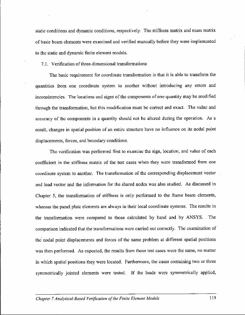
static conditions and dynamic conditions, respectively. The stiffness matrix and mass matrix
of basic beam elements were examined and verified manually before they were implemented
to the static and dynamic finite element models.
7.1. Verification of three-dimensional transformations
The basic requirement for coordinate transformation is that it is able to transform the
quantities from one coordinate system to another without introducing any errors and
inconsistencies. The locations and signs of the components of one quantity may be modified
through the transformation, but this modification must be correct and exact. The value and
accuracy of the components in a quantity should not be altered during the operation. As a
result, changes in spatial position of an entire structure have no influence on its nodal point
displacements, forces, and boundary conditions.
The verification was performed first to examine the sign, location, and value of each
coefficient in the stiffness matrix of the test cases when they were transformed from one
coordinate system to another. The transformation of the corresponding displacement vector
and load vector and the information for the shared nodes was also studied. As discussed in
Chapter 5, the transformation of stiffness is only performed to the frame beam elements,
whereas the panel plate elements are always in their local coordinate systems. The results in
the transformation were compared to those calculated by hand and by A N S Y S . The
comparison indicated that the transformations were carried out correctly. The examination of
the nodal point displacements and forces of the same problem at different spatial positions
was then performed. As expected, the results from those test cases were the same, no matter
in which spatial positions they were located. Furthermore, the cases containing two or three
symmetrically jointed elements were tested. If the loads were symmetrically applied,
Chapter 7 Analytical-Based Verification of the Finite Element Models 119

symmetric nodal point displacements and forces were obtained. If the loads were anti
symmetrically applied, the structure rotated about its center of gravity. A few examples of
the test cases are shown in Figure 7.1.
Figure 7.1 Test cases used in verifications
Chapter 7 Analytical-Based Verification of the Finite Element Models 120

7.2. Verification of the static finite element model
The static finite element model was verified by running a group of linear cantilever
beams with varied cross-sectional shapes in three-dimensional space and then comparing the
results with mechanics theory. The beams actually were built-up systems due to the nature of
the element unit implemented in the model. The results would reflect the contributions from
all three types of elements. Therefore, the results given by the current finite element model
and the one from classical beam theory may not be comparable directly i f the cases used in
the theoretical calculations were only constructed by one type of member with homogeneous
material property. To configure an approximate uniform and homogeneous system, only one
type of element, for example panel element, was considered at one time by minimizing the
contribution of the other elements. This can be easily done by appropriately selecting the
parameters of panel, frame, and nail connections. In this way, the panel element and frame
element in the model can also be examined separately. To make the comparison of the
results from both the numerical and the theoretical procedures available, it is essential for the
test case to yield a linear response. This was achieved by limiting the nail deformation
within its linear elastic region.
7.2.1. Linear cantilever beams
In constructing linear cantilever beams with dominant panel element properties, low
Young's modulus values and small cross-section dimensions were applied to the frame
members so that the stiffness of frame member was negligible and therefore the panel would
carry the loads solely., In addition, a high nail initial stiffness K was required to ensure the
frame members being tightly fixed on the panel member to eliminate relative movement
between them. The Young's moduli in x andy directions (Ex and Ey) were assigned the same
Chapter 7 Analytical-Based Verification of the Finite Element Models 121
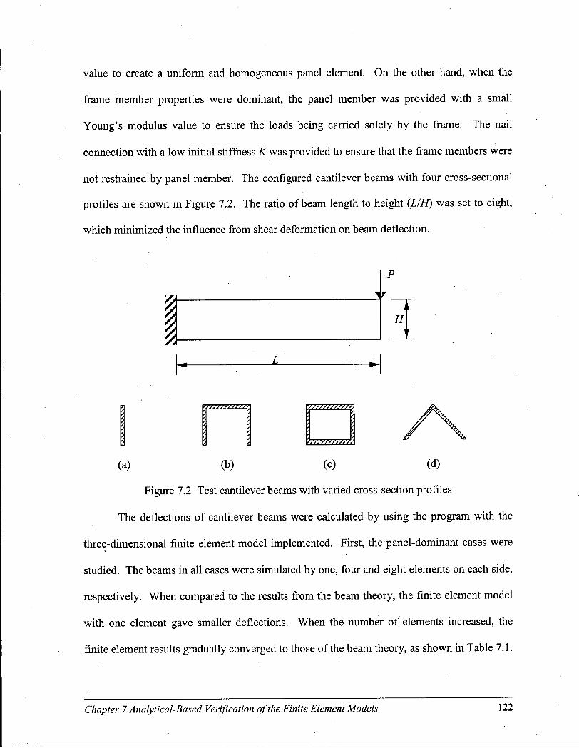
value to create a uniform and homogeneous panel element. On the other hand, when the
frame member properties were dominant, the panel member was provided with a small
Young's modulus value to ensure the loads being carried solely by the frame. The nail
connection with a low initial stiffness K was provided to ensure that the frame members were
not restrained by panel member. The configured cantilever beams with four cross-sectional
profiles are shown in Figure 7.2. The ratio of beam length to height (L/H) was set to eight,
which minimized the influence from shear deformation on beam deflection.
P
(a) (b) (c) (d)
Figure 7.2 Test cantilever beams with varied cross-section profiles
The deflections of cantilever beams were calculated by using the program with the
three-dimensional finite element model implemented. First, the panel-dominant cases were
studied. The beams in all cases were simulated by one, four and eight elements on each side,
respectively. When compared to the results from the beam theory, the finite element model
with one element gave smaller deflections. When the number of elements increased, the
finite element results gradually converged to those of the beam theory, as shown in Table 7.1.
Chapter 7 Analytical-Based Verification of the Finite Element Models 122

(The unit used in all of the following tables is in meter.) The formula from the beam theory
used to calculate the deflection of a cantilever without considering the shear deformation is
Beam theory also tells that when a beam is undergoing an elastic deformation, its
deflection decreases proportionally when increasing its moment of inertia i f its elastic
properties and loading conditions are kept constant. This was demonstrated by comparing
the moments of inertia and deflections in beams (a*) with doubled thickness, (b), (c) and (d)
to those in beam (a), as shown in Table 7.2.
Table 7.1 Comparisons of beam deflections predicted by the finite element model and
calculated by the beam theory - Panel-dominant cases
Cross- No. of Deflection, A
Section Element FE Model Beam Theory
A 1 0.2238 x 10"2 0.3199xl0" 2
4 0.2929 x 10 - 2
8 0.3086 x 10"2
B 1 0.4962 x 10"3 0.6504 x 10"3
4 0.6044 x 10"3
8 0.6504 x 10"3
C 1 0.2134 x 10"3 0.2985 x 10"3
4 0.2905 x 10"3
8 0.2975 x 10"3
D 1 0.2187 x 10"2 0.3078 x 10"2
4 0.2869 x 10"2
8 0.2912 x 10"2
Chapter 7 Analytical-Based Verification of the Finite Element Models 123
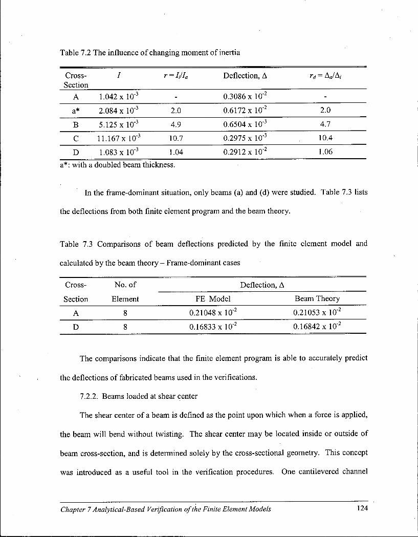
Table 7.2 The influence of changing moment of inertia
Cross-Section
r = lilla Deflection, A rd = A„/A(-
A 1.042 x 10"3 - 0.3086 x 10"2 -
a* 2.084 x 10 - 3 2.0 0.6172 x 10"2 2.0
B 5.125 x 10 - 3 4.9 0.6504 x 10"3 4.7
C 11.167 x 10 - 3 10.7 0.2975 x 10 - 3 10.4
D 1.083 x 10"3 1.04 0.2912 x 10"2 1.06
a*: with a doubled beam thickness.
In the frame-dominant situation, only beams (a) and (d) were studied. Table 7.3 lists
the deflections from both finite element program and the beam theory.
Table 7.3 Comparisons of beam deflections predicted by the finite element model and
calculated by the beam theory - Frame-dominant cases
Cross- No. of Deflection, A
Section Element FE Model Beam Theory
A 8 0.21048 x 10"2 0.21053 x lO - 2
D 8 0.16833 x 10"2 0.16842 x 10"2
The comparisons indicate that the finite element program is able to accurately predict
the deflections of fabricated beams used in the verifications.
7.2.2. Beams loaded at shear center
The shear center of a beam is defined as the point upon which when a force is applied,
the beam will bend without twisting. The shear center may be located inside or outside of
beam cross-section, and is determined solely by the cross-sectional geometry. This concept
was introduced as a useful tool in the verification procedures. One cantilevered channel
Chapter 7 Analytical-Based Verification of the Finite Element Models 124

section and one cantilevered angle section (cross-sections (b) and (d), illustrated in Section
7.2.1, respectively) were adopted in the further testing of the program.
For the cantilevered channel section, a force P was first applied to its shear center, as
shown in Figure 7.3(a). The displacements measured at points 1 to 4 are listed in Table 7.4.
A graphic display output from the program illustrating the deformation of the end of beam is
shown in Figure 7.4(a). The results demonstrated that when the beam was loaded at its shear
center, it underwent only bending without twisting. Secondly, when it was only subjected to
a force P at point 1 (Figure 7.3(b)), the beam showed a deformation at its end caused by both
bending and twisting (Figure 7.4(b)).
1 1
(a) (b)
Figure 7.3 Channel sections were loaded at shear center or at corner 1
Table 7.4 Displacements of four points at the end of beam when loaded at shear center
Point A, A,
1 0.443 x IO"4 0.0
2 0.443 x 10"4 0.0
3 0.436 x 10"4 -0.007 x 10"4
4 0.436 x 10"4 0.007 x IO - 4
Chapter 7 Analytical-Based Verification of the Finite Element Models 125
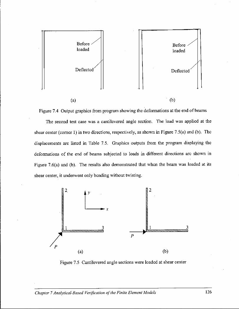
Before loaded
Before loaded
V Deflected Deflected
(a) (b)
Figure 7.4 Output graphics from program showing the deformations at the end of beams
The second test case was a cantilevered angle section. The load was applied at the
shear center (corner 1) in two directions, respectively, as shown in Figure 7.5(a) and (b). The
displacements are listed in Table 7.5. Graphics outputs from the program displaying the
deformations of the end of beams subjected to loads in different directions are shown in
Figure 7.6(a) and (b). The results also demonstrated that when the beam was loaded at its
shear center, it underwent only bending without twisting.
2 2 y
1 3 1 3
P
(a) (b)
Figure 7.5 Cantilevered angle sections were loaded at shear center
Chapter 7 Analytical-Based Verification of the Finite Element Models 126
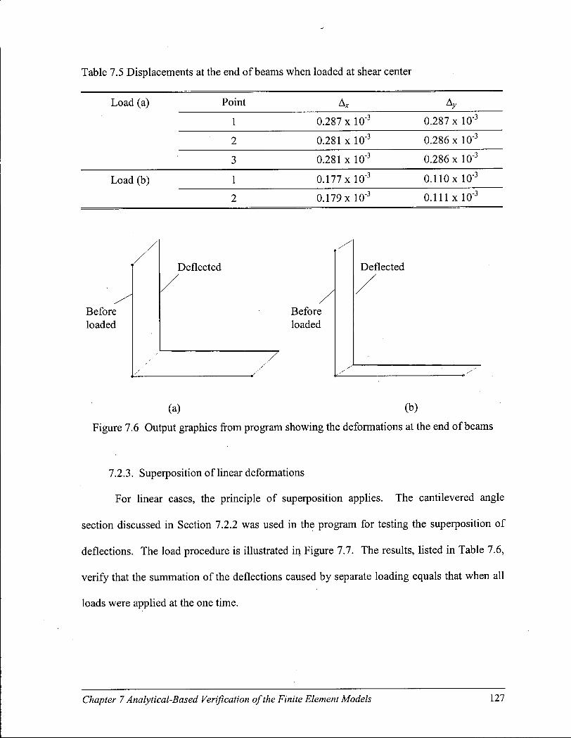
Table 7.5 Displacements at the end of beams when loaded at shear center
Load (a) Point Ax Ay
1 0.287 x 10"3 0.287 x 10 - 3
2 0.281 x 10'3 0.286 x 10"3
3 0.281 x 10"3 0.286 x 10"3
Load (b) 1 0.177 x 10"3 0.110 x 10"3
2 0.179 x lO" 3 0.111 x lO" 3
Before loaded
Deflected
Before loaded
Deflected
(a) (b)
Figure 7.6 Output graphics from program showing the deformations at the end of beams
7.2.3. Superposition of linear deformations
For linear cases, the principle of superposition applies. The cantilevered angle
section discussed in Section 7.2.2 was used in the program for testing the superposition of
deflections. The load procedure is illustrated in Figure 7.7. The results, listed in Table 7.6,
verify that the summation of the deflections caused by separate loading equals that when all
loads were applied at the one time.
Chapter 7 Analytical-Based Verification of the Finite Element Models 127

© +
2 i y
Ik.
©
1
3P
*- X
3P
Figure 7.7 Test of superposition of linear deformations
Table 7.6 Superposition of displacements
Point Direction A of Step © A of Step © © + © A of Step ©
1 X 0.177 x 10"3 0.331 x 10"3 0.508 x 10"3 0.508 x 10"3
Y 0.110 x 10"3 0.531 x 10"3 0.641 x IO"3 0.641 x IO"3
2 X 0.180 x IO - 3 0.304 x 10"3 0.484 x IO"3 0.484 x 10"3
Y 0.111 x 10"3 0.526 x 10"3 0.637 x 10"3 0.637 x IO"3
7.2.4. Stresses in cantilever beams
Stresses in the beam (a) (Figure 7.2, Section 7.2.1) with 8 elements obtained from the
finite element program were compared with stresses obtained from the beam theory. The
stresses calculated by the beam theory were taken from the middle line along the r\ axis,
whereas the stresses calculated by the finite element program were obtained by averaging the
results from the two middle columns of Gauss points (Figure 7.8). The unit of the stresses is
kN/m 2 . The beam theory assumes that there is no interaction between two horizontal layers
in a cantilever beam and therefore gives zero normal stress iny direction (cy = 0). In finite
element analysis, the stresses are calculated from strains at Gauss points in each discrete
element based on the relationships from Hooke's law (see Equation (4.6)). These
Chapter 7 Analytical-Based Verification of the Finite Element Models 128

relationships describe that normal stress in y direction (cy) is a function of normal strain in x
direction (ex)- Therefore, in each individual element, ay is no longer zero.
5=-0.861... 5=-0.339...
n=0.861..
r|=0.339...
ri=-0.339r-
•n=-0.861—
5=0.339... 5=0.861.
Figure 7.8 The locations of Gauss Points in one element
The beam theory uses the following formulas to calculate the normal and shear
stresses:
PL
PQ It
(7.2)
(7,3)
o =
The beam theory gives:
' 773.75 670.59 567.42 305.90 265.12 224.33
-305.90 -265.12 -224.33 -183.54 -142.75 -773.75 -670.59' -567.42 -464.25 -361.08
464.25 183.54
361.08 142.75
257.92 101.97
-101.97 -257.92
154.75 61.18
-61.18
51.58 20.39
-20.39
•154.75 -51.58
a r = 0
Chapter 7 Analytical-Based Verification of the Finite Element Models 129
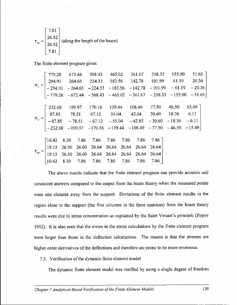
T = xy
7.81 26.52 26.52 7.81
(along the length of the beam)
The finite element program gives:
a -
779.28 294.91
-294.91 -779.28
' 232.68 87.85.
-87.85
672.44 568.43 264.65 224.33
-264.65 -224.33
465.02 183.56
361.67 142.78
258.33 101.99
155.00 61.19
183.56 -142.78 -101.99 -61.19
51.65 20.36
-20.36
672.44 -568.43 -465.02 -361.67 -258.33 -155.00 -51.65
199.97 78.51
-78.51
170.16 67.12
-67.12
139.44 55.04
-55.04
108.49 42.04
-42.83
-232.68 -199.97 -170.16 -139.44 -108.49
77.50 46.50 15.49 30.60 18.36 6.11
-30.60 -18.36 -6.11 -77.50 -46.50 -15.49
x = xy
10.42 8.30 7.86 7.86 7.86 7.86 7.86 7.86
19.15 26.50 26.60 26.64 26.64 26.64 26.64 26.64
19.15 26.50 26.60 26.64 26.64 26.64 26.64 26.64
10.42 8.30 7.86 7.86 7.86 7.86 7.86 7.86
The above results indicate that the finite element program can provide accurate and
consistent answers compared to the output from the beam theory when the measured points
were one element away from the support. Deviations of the finite element results in the
region close to the support (the first columns in the three matrices) from the beam theory
results were due to stress concentration as explained by the Saint Venant's principle (Popov
1952). It is also seen that the errors in the stress calculations by the finite element program
were larger than those in the deflection calculations. The reason is that the stresses are
higher order derivatives of the deflections and therefore are prone to be more erroneous.
7.3. Verification of the dynamic finite element model
The dynamic finite element model was verified by using a single degree of freedom
Chapter 7 Analytical-Based Verification of the Finite Element Models 130
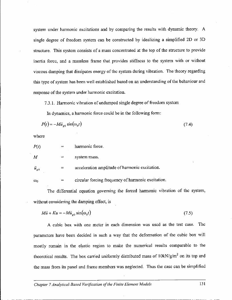
system under harmonic excitations and by comparing the results with dynamic theory. A
single degree of freedom system can be constructed by idealizing a simplified 2D or 3D
structure. This system consists of a mass concentrated at the top of the structure to provide
inertia force, and a massless frame that provides stiffness to the system with or without
viscous damping that dissipates energy of the system during vibration. The theory regarding
this type of system has been well established based on an understanding of the behaviour and
response of the system under harmonic excitation.
7.3.1. Harmonic vibration of undamped single degree of freedom system
In dynamics, a harmonic force could be in the following form:
P{t) = -Mug0 sin(ov) (7.4)
where
P(t) = harmonic force.
M = system mass.
ug0 = acceleration amplitude of harmonic excitation.
coo = circular forcing frequency of harmonic excitation.
The differential equation governing the forced harmonic vibration of the system,
without considering the damping effect, is
Mix + Ku = -Miig0 sin(co0/) (7.5)
A cubic box with one meter in each dimension was used as the test case. The
parameters have been decided in such a way that the deformation of the cubic box will
mostly remain in the elastic region to make the numerical results comparable to the
theoretical results. The box carried uniformly distributed mass of lOkN/g/m on its top and
the mass from its panel and frame members was neglected. Thus the case can be simplified
Chapter 7 Analytical-Based Verification of the Finite Element Models 131
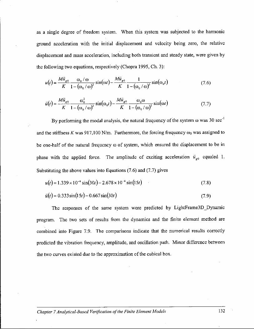
as a single degree of freedom system. When this system was subjected to the harmonic
ground acceleration with the initial displacement and velocity being zero, the relative
displacement and mass acceleration, including both transient and steady state, were given by
the following two equations, respectively (Chopra 1995, Ch. 3):
"(0 = J , / , vs i n M vsin((Oo0 (7.6)
A 1 - (co0 /co) A 1 - (co0 / C O )
M i 0 co2 • / \ ^ " s o O0C0 . / \
A 1 - (C0 0 /COJ A l-(t0 0/C0)
By performing the modal analysis, the natural frequency of the system co was 30 sec"1
and the stiffness AT was 917,100 N/m. Furthermore, the forcing frequency coo was assigned to
be one-half of the natural frequency co of system, which ensured the displacement to be in
phase with the applied force. The amplitude of exciting acceleration ug0 equaled 1.
Substituting the above values into Equations (7.6) and (7.7) gives
u(t) = 1.339 xl0 _ 4 s in(30f)- 2.678 x 10"4 sin(l5r) (7.8)
u(t) = 0.333 sin(l 5t) - 0.667 sin(30f) (7.9)
The responses of the same system were predicted by LightFrame3D_Dynamic
program. The two sets of results from the dynamics and the finite element method are
combined into Figure 7.9. The comparisons indicate that the numerical results correctly
predicted the vibration frequency, amplitude, and oscillation path. Minor difference between
the two curves existed due to the approximation of the cubical box.
Chapter 7 Analytical-Based Verification of the Finite Element Models 132

Time (sec)
(a) Displacement-time history
-1.0 ' 0.0 0.5 1.0 1.5 2.0 2.5 3.0 3.5 4.0 4.5 5.0
Time (sec)
(b) Acceleration-time history
Figure 7.9 Comparisons of responses of an undamped single degree of freedom system
between theoretical calculation and numerical prediction
7.3.2. Harmonic vibration of damped single degree of freedom system
The differential equation governing the forced harmonic vibration of the system,
considering the damping effect, is
Mil + Cii + Ku = -Miig0 sin(co0f) (7.10)
where C is viscous damping coefficient.
The responses of the system to the harmonic excitation including both transient and
steady state are:
Chapter 7 Analytical-Based Verification of the Finite Element Models 133

u(t) = e'^'A sin(co/) - B sin(oy) + D cos(a>0f) (7.11)
u{f)=e^Asm{<Qit%C3<ay - co^]+5co2 sin(co0f)-Deo2 cos(co0f) (7.12)
where
Mug0 co„ / co A = *- f (7.13)
K l - ( c o 0 / c o ) 2
B = ̂ r ^ (7-14) K [ l - ( c o 0 / c o ) 2 f + [ 2 ^ ( c o 0 / c o ) ] 2
D_Mug0 2 C ( c o 0 / c o )
K [ l - K / c o y f + ^ k / c o ) ] 2
co r f = coVl-C 2 (7.16)
For the same cubic box used in Section 7.3.1, assuming the damping ratio C, to be 5%,
Equations (7.11) and (7.12) become
u{t) = e - 3 5 2 8'1.339 x 1(T4 sin(70.472f)- 2.666 x 10 - 4 sin(35.280
+1.777 xlCT5cos(35.28f) ( ? ' 1 7 )
„•(/) = e - 3 5 2 8 ' (_ 0.663)sin(70.472?) + 0.332 sin(35.28f) - 0.022 cos(35.28t) (7.18)
Comparison of the results from dynamics and the finite element program is shown in
Figure 7.10. Excellent agreements were achieved.
(a) Displacement-time history
Chapter 7 Analytical-Based Verification of the Finite Element Models 134
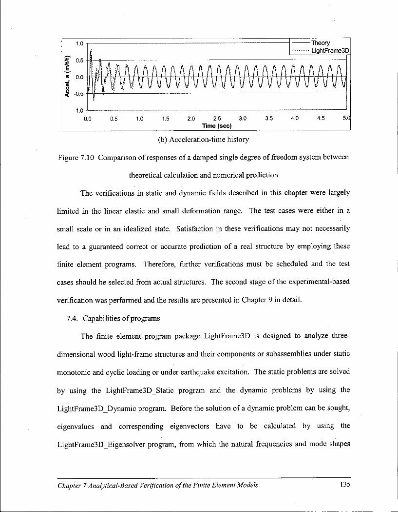
(b) Acceleration-time history
Figure 7.10 Comparison of responses of a damped single degree of freedom system between
theoretical calculation and numerical prediction
The verifications in static and dynamic fields described in this chapter were largely
limited in the linear elastic and small deformation range. The test cases were either in a
small scale or in an idealized state. Satisfaction in these verifications may not necessarily
lead to a guaranteed correct or accurate prediction of a real structure by employing these
finite element programs. Therefore, further verifications must be scheduled and the test
cases should be selected from actual structures. The second stage of the experimental-based
verification was performed and the results are presented in Chapter 9 in detail.
7.4. Capabilities of programs
The finite element program package LightFrame3D is designed to analyze three-
dimensional wood light-frame structures and their components or subassemblies under static
monotonic and cyclic loading or under earthquake excitation. The static problems are solved
by using the LightFrame3D_Static program and the dynamic problems by using the
LightFrame3D_Dynamic program. Before the solution of a dynamic problem can be sought,
eigenvalues and corresponding eigenvectors have to be calculated by using the
LightFrame3D_Eigensolver program, from which the natural frequencies and mode shapes
Chapter 7 Analytical-Based Verification of the Finite Element Models 135
of the system can be derived. To accurately simulate the actual behaviour of wood
structures, both material nonlinearity and geometric nonlinearity are considered in the finite
element modeling. The former is associated with changes in material properties, as in the
nail connections, and the latter is associated with changes in configuration, as in the large
deflections (P-A behaviour) of panel and frame members.
LighfFrame3D programs try to address the common building configurations and
loading conditions in a versatile manner. The programs are capable of analysing structures
with the following features:
(1) The components in a system can be either single side sheathed or double side sheathed
with or without insulation material applied. When double side sheathed, the material
properties and dimensions of panels on one side may be different from the other side.
The nail connections on two sides may also have varied configurations.
(2) The material properties and dimensions of frame members along four edges of one
element can be different. In some situations when sharing frame members occurs, one
element may have only one or two or three frame members i f those members are
accounted by other elements.
(3) On each frame member, nail connections can be in different type, including material
properties, size, and spacing. In general, nail connections behave nonlinearly. Any nail
line must have a frame member to match it. In some cases, it is desirable to give linear
properties to the nail connections in a number of elements which are not at the critical
positions. This may simplify the model, especially of a large problem, to save a
significant amount of computational time.
(4) In the static analysis, in-plane concentrated loads and out-of-plane distributed loads can
Chapter 7 Analytical-Based Verification of the Finite Element Models 136

be applied simultaneously. These loads may be constant or incremented individually in
fixed or uneven steps. Load control mode or displacement control mode is used as input
history in static monotonic analysis, whereas only displacement control mode is used in
static cyclic analysis. In the dynamic analysis, the earthquake excitations can be assigned
in horizontal and/or vertical directions and the static constant loads can be applied to the
structure at the same time.
(5) Window and door openings can be located on a component in different sizes and
locations.
(6) There is no limitation on the problem size and the number of elements from the program
code because of the use of dynamically allocated arrays. The problem size as well as the
computational time, however, largely depends on the capacity of a computer system to be
used and the nature of the problem.
The programs are built with three major modules: preprocessor, solution, and
postprocessor. The preprocessor generates appropriate text and graphic files to allow the
user to review the input data and mesh information prior to execution of the solution
procedure. The computational effectiveness and accuracy are based on a well-constructed
model. Material properties, nail connection types, loading schemes and boundary conditions
in the model must be correctly defined. Different element sizing, nodal numbering and
meshing patterns could be tested to investigate the model sensitivity and stabilization. The
model should be checked by closely reviewing all the information in the text files and
graphic files provided by the preprocessor. For large problems, the graphic display provided
by the programs is preferable because the errors in input data files can be easily detected
from the visualized graphs. Such common errors in input data include misplaced nodes or
Chapter 7 Analytical-Based Verification of the Finite Element Models 137

their coordinates, incorrectly numbered elements, misapplied boundary conditions, and loads.
Before conclusions can be drawn from the solution procedures, the most important
step is to review all the results generated by the postprocessor based on engineering
judgments. These results are in the form of text and graphic files detailing local and global
deformation and force information and displaying visualized step-by-step structural
deformation. The text files include nodal displacements and forces in six degrees of
freedom, panel normal and shear stresses, maximum nail forces and locations, nail bending
and withdrawal deformations, and relative movement between frame and panel members.
The tearing failure at panel edges due to nail compression and maximum bending stress in
frame members are also given i f they need to be checked. The graphic files show the
deformed shape of the structure being modeled in each step (in the static analysis) or selected
steps (in the dynamic analysis). A set of slides is also produced to display an entire
continuous load-deformation course of the structure. Detailed user procedures of the
programs are presented in Appendix A .
Chapter 7 Analytical-Based Verification of the Finite Element Models 138

CHAPTER 8
PROCEDURES OF EXPERIMENTAL STUDY ON SIMPLIFIED THREE-DIMENSIONAL BUILDINGS
As an integral component of the numerical modeling of three-dimensional wood-
frame buildings, an experimental study was proposed, organized and conducted. The study
contained a group of laboratory tests on full-scale simplified three-dimensional 2 by 4 light-
frame structures. They were of realistic size and scale, but not installed to represent a real
house. The main objective of the experimental study was to provide comprehensive test
results required in the verifications of finite element models. These tests can also provide an
opportunity for researchers to physically observe the actual behaviour of simplified wood
light-frame buildings under static loading and dynamic excitation. This chapter introduces
the test facilities for this study with the description of test setup and input signal generating
and collecting system. It presents in detail the procedures in determining the test models and
their structural components with the help of programs. The test results will be given in
Chapters 9 and 10, integrated into the experimental-based model verification procedures.
8.1. Test facility
A l l of the static and dynamic tests were conducted on the shake table in the
Earthquake Engineering Laboratory in the Department of Civi l Engineering at U B C . The
test buildings were mounted on a base frame that was attached to the surface of the table.
The entire test facility consisted of shake table, test base frame, inertial mass, computer
Chapter 8 Procedures of Experimental Study on Simplified Three-Dimensional Buildings 139

control system, and data acquisition system. The test base frame, composed of steel I-beams
and channels, was designed after the dimensions of test buildings had been determined.
8.1.1. Capacity of shake table
The shake table is a 3 x 3 m aluminum cellular structure, capable of simulating
multiple-directional earthquakes. In the tests, one of the configurations of the shake table
mechanism, 3H, was used. This mechanism generated only horizontal motions, from which
two translational motions and one rotational motion can be simulated. Under this
configuration, the vertical supports acted as rigid links. For clarity, the direction running in
East and West was defined as the primary direction, represented by x, and the direction
running in North and South as the secondary direction, represented by y, as shown in Figure
8.1. The horizontal motion in the primary direction was produced by a table actuator with a
maximum load capacity of 156 kN and a maximum displacement of ±76 mm ( A l in Figure
8.1). In the bi-directional dynamic test, the horizontal motions perpendicular to the primary
motion were generated by two additional actuators located in the south side of the table (A2
and A3 in Figure 8.1). The motions of the shake table were controlled by specialized
software which performed a closed-loop control to reproduce recorded earthquake motions
with high accuracy. A data acquisition system with 32 channels was equipped for recording
the responses from test specimen.
8.1.2. Data acquisition system
A total of 28 channels in the data acquisition system were employed to measure
loads, displacements, and acceleration signals during tests. Figure 8.1 illustrates their
positions.
In the static tests, one load cell (Gl) with 45 kN load capacity was fixed in between
Chapter 8 Procedures of Experimental Study on Simplified Three-Dimensional Buildings 140

the rigid arm from a reaction frame and the steel beam connected to the top of the test
building to measure the load that the building was subjected to. One Linear Variable
Displacement Transducer (LVDT) (DI), mounted on the actuator A l , was used to measure
the displacement of the shake table in the loading direction. Three LVDTs in the x direction
( B l , B2 and B3) and two in the y direction (B4 and B5) were installed to measure the
displacements on the top of the test building. The data from those LVDTs were also used to
calculate the building torsional motion. Two dial gauges were vertically mounted at two
eastside base corners to obtain the uplift readings of end frame members, assigned as C l and
C2. In addition, two LVDTs (FI and F2) were installed diagonally on both the north and
south shear walls to measure the diagonal displacements, which may help to determine shear
wall deformation.
In the dynamic tests, besides using the above-mentioned transducers for displacement
measurements, four accelerometers (El to E4) were mounted at the center and corners of the
top of the test building to monitor the resultant acceleration signals in the building in the
primary (_p) and secondary (_s) directions. Two accelerometers were also used to measure
the table accelerations in both directions. The dial gauges (C l and C2) were replaced by
transducers, and two more transducers (C3 and C4) were added to measure dynamic uplifts.
In the bi-directional dynamic test, two LVDTs (D2 and D3) mounted on actuators A2 and A3
measured the displacements of the shake table in the secondary direction. MTS Seismic
Shock Simulation System and Data Acquisition System were used to regenerate the
earthquake signals and record the test signals.
The sampling frequency was 50 readings per second in the static tests and 200
readings per second in the dynamic tests.
Chapter 8 Procedures of Experimental Study on Simplified Three-Dimensional Buildings 141

t South
A2&D2 A3&D3 E6
East
B4 — i
B3
A1&D1
G1,E5
B2,
E6 • i tl C2
E3_p E4_p
E3_s
BI
E2_s
E4 s
E l s El_p
C l
E2_p Test building
Shake table F l
B5
West
C4
North
Figure 8.1 Data acquisition layout (plan view)
8.2. Determination of test buildings
The testing specimens were predetermined to be a few full-scale one-storey 2 by 4
light-frame simplified box-type models with a rectangular plan. They would have four walls
and one roof, built with commonly used construction materials. Due to the limitation of
shake table space, the dimensions of test models were restricted to 3.048 m (10 ft.) in the x
direction x 2.438 m (8 ft.) in the y direction x 2.438 m in height. Accordingly, the structural
details of the test models need to be scaled so that the data for the model verifications can be
obtained, while the maximum loading capacity of the shake table would not be exceeded.
The tests need to provide the following information:
(1) Load-displacement characteristics under static loading condition;
(2) Natural frequencies and mode shapes under free vibration condition;
(3) Dynamic response under ground excitation;
(4) Torsional response under both static and dynamic loading; and
Chapter 8 Procedures of Experimental Study on Simplified Three-Dimensional Buildings 142
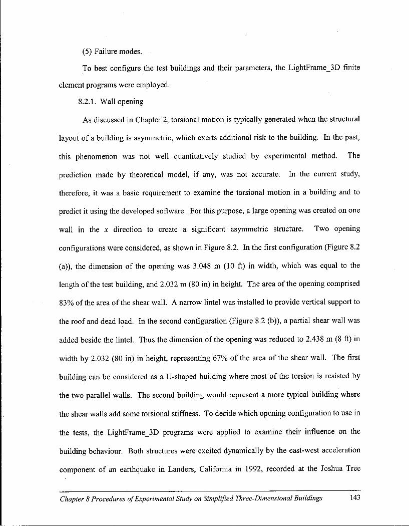
(5) Failure modes.
To best configure the test buildings and their parameters, the LightFrame_3D finite
element programs were employed.
8.2.1. Wall opening
As discussed in Chapter 2, torsional motion is typically generated when the structural
layout of a building is asymmetric, which exerts additional risk to the building. In the past,
this phenomenon was not well quantitatively studied by experimental method. The
prediction made by theoretical model, i f any, was not accurate. In the current study,
therefore, it was a basic requirement to examine the torsional motion in a building and to
predict it using the developed software. For this purpose, a large opening was created on one
wall in the x direction to create a significant asymmetric structure. Two opening
configurations were considered, as shown in Figure 8.2. In the first configuration (Figure 8.2
(a)), the dimension of the opening was 3.048 m (10 ft) in width, which was equal to the
length of the test building, and 2.032 m (80 in) in height. The area of the opening comprised
83% of the area of the shear wall. A narrow lintel was installed to provide vertical support to
the roof and dead load. In the second configuration (Figure 8.2 (b)), a partial shear wall was
added beside the lintel. Thus the dimension of the opening was reduced to 2.438 m (8 ft) in
width by 2.032 (80 in) in height, representing 67% of the area of the shear wall. The first
building can be considered as a U-shaped building where most of the torsion is resisted by
the two parallel walls. The second building would represent a more typical building where
the shear walls add some torsional stiffness. To decide which opening configuration to use in
the tests, the LightFrame_3D programs were applied to examine their influence on the
building behaviour. Both structures were excited dynamically by the east-west acceleration
component of an earthquake in Landers, California in 1992, recorded at the Joshua Tree
Chapter 8 Procedures of Experimental Study on Simplified Three-Dimensional Buildings 143
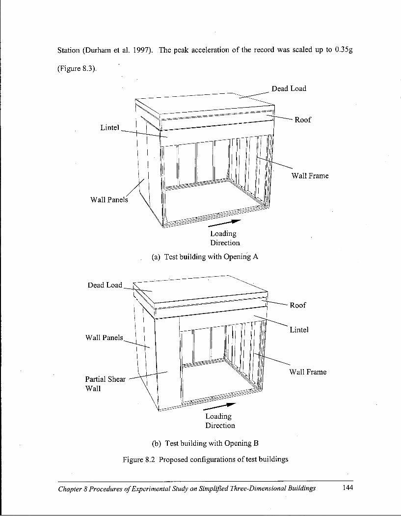
Station (Durham et al. 1997). The peak acceleration of the record was scaled up to 0.35g
(Figure 8.3).
Dead Load
Loading Direction
(a) Test building with Opening A
Loading Direction
(b) Test building with Opening B
Figure 8.2 Proposed configurations of test buildings
Chapter 8 Procedures of Experimental Study on Simplified Three-Dimensional Buildings 144

0.4 0.3
3 0.2 8 0.1
0 -0.1 •o c
P -0.2 -0:3 -0.4
—i—rt tfl —|—: L L | - _ | _ U P
10 15 20 Time (s)
25 30 35 40
Figure 8.3 Joshua Tree record, 1992 California Landers earthquake, 0.35g
Five groups of displacement data on the roof of each test buildings were output by the
program, as shown in Figure 8.4, to fully represent the in-plane and out-of-plane motions of
all the walls and the rigid body lateral motion of the roof. The drifts in the x direction (the
primary direction) measured at point xo on the test building for Openings A and B are
presented in Figure 8.5. The relative drifts in the x (the difference between x\ and x 2 ) and the
y (the difference between y\ and yi) directions for two test buildings are presented in Figure
8.6 and Figure 8.7, respectively. The graphs start from the fifth second, because the
vibrations of the systems during the first five seconds were insignificant.
x 2
X i
Xo r
V2
Roof of test building
Figure 8.4 Locations of displacement measurement for torsion calculation
Chapter 8 Procedures of Experimental Study on Simplified Three-Dimensional Buildings 145
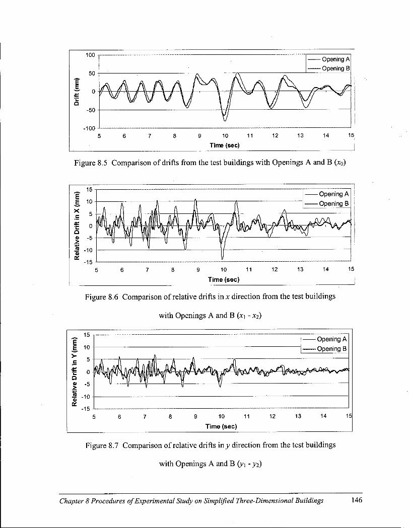
100
-100
Opening A Opening B
8 9 10 11 12 13 14 15|
Time (sec)
Figure 8.5 Comparison of drifts from the test buildings with Openings A and B (x0)
•Opening A
•Opening B
9 10 11
Time (sec)
15
Figure 8.6 Comparison of relative drifts in x direction from the test buildings
with Openings A and B (x\ - xi)
15 T
E E 10
c
i o Q a> .5 1 "10
-15
•Opening A
•Opening B
9 10 11
Time (sec)
12 13 14 15
Figure 8.7 Comparison of relative drifts iny direction from the test buildings
with Openings A and B (yi - yi)
Chapter 8 Procedures of Experimental Study on Simplified Three-Dimensional Buildings 146

As evident in Figure 8.5, the difference between the two predictions in most of the
time period is not significant. The test building with Opening A reached a maximum drift of
81.7 mm and that for the test building with Opening B was 66.3 mm. The relative drifts in
both the x and y directions, however, showed a substantial difference. For example, in the x
direction, the maximum relative drifts in the buildings with Opening A and B were,
respectively, 11.0 mm and 7.2 mm, and in the y direction, they were 6.8 mm and 5.0 mm.
On the other hand, i f considering the ratio of the relative drifts to the absolute drift in each
case, the influence due to the opening on the building torsional motion was at the same level
of significance.
It would not be hard to imagine that the stresses in the top beam and lintel of the test
house with Opening A were greater than those in the house with Opening B when the top
dead load was applied. It is because the former had a longer opening span, whereas in the
latter, the framing studs of the narrow shear wall provided additional support to reduce the
stresses in the members. Based on the information obtained from the predictions by the
program and considering that Opening B was closer to the actual construction layout, the
decision was made to use the Opening B in all of the test buildings.
8.2.2. Structural details of walls in test buildings
When constructed with the standard building configurations and materials, the test
models in the determined dimensions could be much stiffer. Their strength might exceed the
load capacity of the shake table, and their deformation might not reach the expected level.
Thus, the structural details needed to be adjusted to create softened test buildings. The
change, which would be easily implemented to affect the building behaviour, was considered
to be the enlargement in the distance between the framing studs. This change reduced the
Chapter 8 Procedures of Experimental Study on Simplified Three-Dimensional Buildings
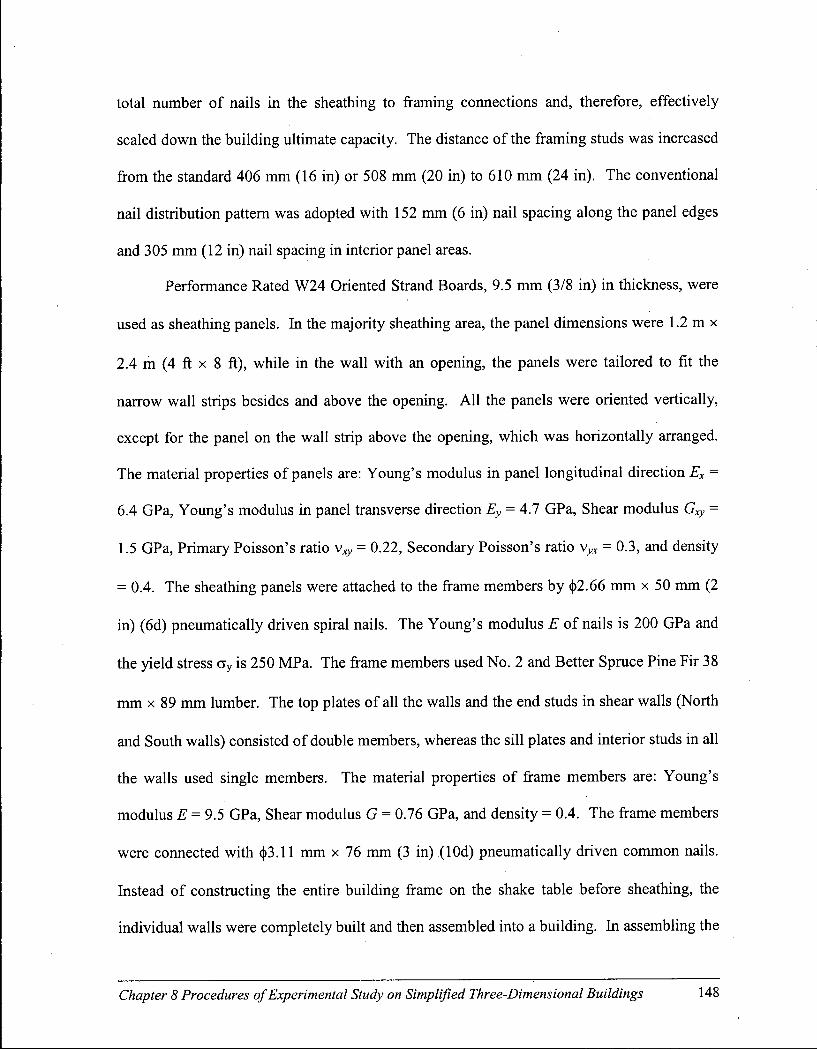
total number of nails in the sheathing to framing connections and, therefore, effectively
scaled down the building ultimate capacity. The distance of the framing studs was increased
from the standard 406 mm (16 in) or 508 mm (20 in) to 610 mm (24 in). The conventional
nail distribution pattern was adopted with 152 mm (6 in) nail spacing along the panel edges
and 305 mm (12 in) nail spacing in interior panel areas.
Performance Rated W24 Oriented Strand Boards, 9.5 mm (3/8 in) in thickness, were
used as sheathing panels. In the majority sheathing area, the panel dimensions were 1.2 m x
2.4 m (4 ft x 8 ft), while in the wall with an opening, the panels were tailored to fit the
narrow wall strips besides and above the opening. A l l the panels were oriented vertically,
except for the panel on the wall strip above the opening, which was horizontally arranged.
The material properties of panels are: Young's modulus in panel longitudinal direction Ex =
6.4 GPa, Young's modulus in panel transverse direction Ey = 4.7 GPa, Shear modulus Gxy =
1.5 GPa, Primary Poisson's ratio = 0.22, Secondary Poisson's ratio vyx = 0.3, and density
= 0.4. The sheathing panels were attached to the frame members by ct>2.66 mm x 50 mm (2
in) (6d) pneumatically driven spiral nails. The Young's modulus E of nails is 200 GPa and
the yield stress a y is 250 MPa. The frame members used No. 2 and Better Spruce Pine Fir 38
mm x 89 mm lumber. The top plates of all the walls and the end studs in shear walls (North
and South walls) consisted of double members, whereas the sill plates and interior studs in all
the walls used single members. The material properties of frame members are: Young's
modulus E = 9.5 GPa, Shear modulus G = 0.76 GPa, and density = 0.4. The frame members
were connected with <j>3.11 mm x 76 mm (3 in) (lOd) pneumatically driven common nails.
Instead of constructing the entire building frame on the shake table before sheathing, the
individual walls were completely built and then assembled into a building. In assembling the
Chapter 8 Procedures of Experimental Study on Simplified Three-Dimensional Buildings 148
building, the single end studs of the end walls (East and West walls) were firmly nailed to the
end studs of the shear walls (North and South walls). The panel edges in the end walls (East
and West walls) were nailed to the end studs of the shear walls with 152 mm (6 in) nail
spacing. Hold-downs were applied at four corners of the building and at the opening end
stud. In the finite element model, the hold-downs are treated as "rigid connections". A more
sophisticated approach is to consider the hold-downs as non-rigid connections and use
nonlinear springs to represent them. Implementation of nonlinear springs as future
improvement of the model is discussed in Sections 9.3 and 9.4. The material properties for
panels, frame members and nails given in this paragraph were used in the entire numerical
predictions and analyses.
Figure 8.8 presents framing and sheathing details of shear walls and end walls.
609.6 (24) 609.6 (24) 609.6 (24)
3048(120)
(a) Front (North) shear wall with opening
Chapter 8 Procedures of Experimental Study on Simplified Three-Dimensional Buildings 149

609.6 (24) 609.6 (24)
3048 (120)
2. in
(b) Back (South) shear wall
609.6 (24)
2438.4 (96)
520.7 (20 1/2)
2260.6 (89)
—|Jr I
(c) East and West end walls
Figure 8.8 Wall frame and panel layouts
Chapter 8 Procedures of Experimental Study on Simplified Three-Dimensional Buildings 150

8.2.3. Structural details of roof in test buildings
The roof in a test building plays an important role in transferring the forces resulted
from the inertia mass on the top to the foundation and in keeping the integrity of the building
by holding the vertical components. In the current study, it was expected that the roof should
be constructed with enough rigidity to support excessive dead load applied to the building.
The roof had dimensions of 2.4 m (8 ft) by 3.05 m (10 ft), composed of 38 mm (2 in)
x 235 mm (10 in) Douglas Fir joists and 19 mm (3/4 in) Douglas Fir Plywood (Figure 8.9).
Six evenly distributed boards running in the north-south direction were connected to two
continuous end boards with q>3.11 mm x 76 mm (3 in) (lOd) pneumatically driven common
nails. Along the span of the joists, three bracing blocks were nailed to the joists with the
same type of nails. Three plywood panels, two pieces of 1.2 m (4 ft) x 2.4 m (8 ft) plus one
piece of 0.6 m (2 ft) x 2.4 m (8 ft) in the middle, were attached to the roof frame with glue
and floor screws. The panels were oriented in the north-south direction (perpendicular to the
loading direction).
Chapter 8 Procedures of Experimental Study on Simplified Three-Dimensional Buildings 151

3048 (120)
609.6 (24) 609.6 (24) 1219.2 (48)
i 1
I I! i
609.
6 (2
4)
r \----------------~-\ U========i !==========!
609.
5 (2
4)
Figure 8.9 Plan view of roof construction
The Simpson Strong-Tie® light gauge reinforcing angles (A in Figure 8.10) were
nailed to each corner of the joist and the bracing block to provide additional strength. During
the tests, the roof was very tightly connected to all of the four walls by means of 18 Simpson
Strong-Tie® reinforcing angles along the outskirts of the roof in each bay (B in Figure 8.10).
These angles were bolted to the roof joists and the top plates of walls by using two 9.5 mm
(3/8 in) bolts on each face. The reason to apply this unusual roof-to-wall connection was
because it was crucial to the entire test to prevent any relative movement between the roof
and the walls.
Chapter 8 Procedures of Experimental Study on Simplified Three-Dimensional Buildings 152

Figure 8.10 Joint reinforcement
8.2.4. The gravity load applied to test buildings
The design of wood frame houses requires that the roof/floor diaphragm should be
capable of supporting a uniformly distributed gravity load of 4.8 kN-m"2 (100 lb-ft"2). The
load represents the combination of the weight of the structure and furnishings (dead loads),
and snow, rain, and/or occupants (live loads). The current design code requires that when
subjected to earthquake ground motion, the building carrying this designated load should not
collapse. In the future performance-based design code, the design criterion may require that
the building not experience any considerable damage. In the proposed dynamic testing, in
order to generate adequate inertia force to cause significant displacement and damage in test
buildings, the gravity load needed to be increased. In the early stage of designing the test
buildings, besides considering the size of the shake table, the dimensions of the existing steel
plates in the laboratory as the gravity load were also taken into account in determining the
roof area. There were sixteen pieces of steel plates available. They were 1.5 m (59 in) in
Chapter 8 Procedures of Experimental Study on Simplified Three-Dimensional Buildings 153
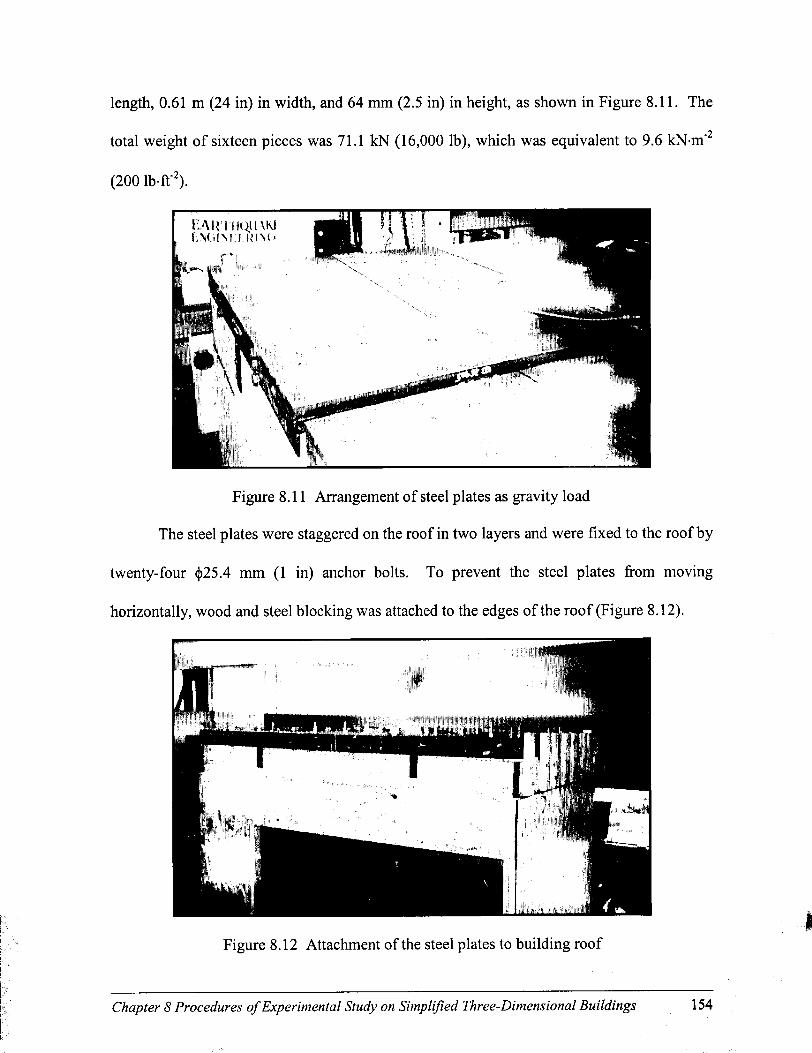
length, 0.61 m (24 in) in width, and 64 mm (2.5 in) in height, as shown in Figure 8.11. The
total weight of sixteen pieces was 71.1 kN (16,000 lb), which was equivalent to 9.6 kN-m"2
(200 lb-fr 2).
Figure 8.11 Arrangement of steel plates as gravity load
The steel plates were staggered on the roof in two layers and were fixed to the roof by
twenty-four (j)25.4 mm (1 in) anchor bolts. To prevent the steel plates from moving
horizontally, wood and steel blocking was attached to the edges of the roof (Figure 8.12).
Figure 8.12 Attachment of the steel plates to building roof
Chapter 8 Procedures of Experimental Study on Simplified Three-Dimensional Buildings 154
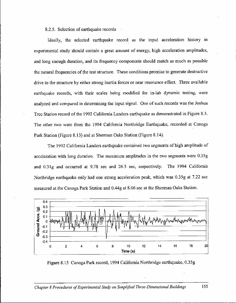
8.2.5. Selection of earthquake records
Ideally, the selected earthquake record as the input acceleration history in
experimental study should contain a great amount of energy, high acceleration amplitudes,
and long enough duration, and its frequency components should match as much as possible
the natural frequencies of the test structure. These conditions promise to generate destructive
drive to the structure by either strong inertia forces or near resonance effect. Three available
earthquake records, with their scales being modified for in-lab dynamic testing, were
analyzed and compared in determining the input signal. One of such records was the Joshua
Tree Station record of the 1992 California Landers earthquake as demonstrated in Figure 8.3.
The other two were from the 1994 California Northridge Earthquake, recorded at Canoga
Park Station (Figure 8.13) and at Sherman Oaks Station (Figure 8.14).
The 1992 California Landers earthquake contained two segments of high amplitude of
acceleration with long duration. The maximum amplitudes in the two segments were 0.35g
and 0.3lg and occurred at 9.78 sec and 26.5 sec, respectively. The 1994 California
Northridge earthquake only had one strong acceleration peak, which was 0.35g at 7.22 sec
measured at the Canoga Park Station and 0.44g at 8.06 sec at the Sherman Oaks Station.
0.4
O) 0.3 -0.2 -
2 -0.2 -
-0.4 0 2 4 6 8 10
Time (s) 12 14 16 18 20
Figure 8.13 Canoga Park record, 1994 California Northridge earthquake, 0.35g
Chapter 8 Procedures of Experimental Study on Simplified Three-Dimensional Buildings 155
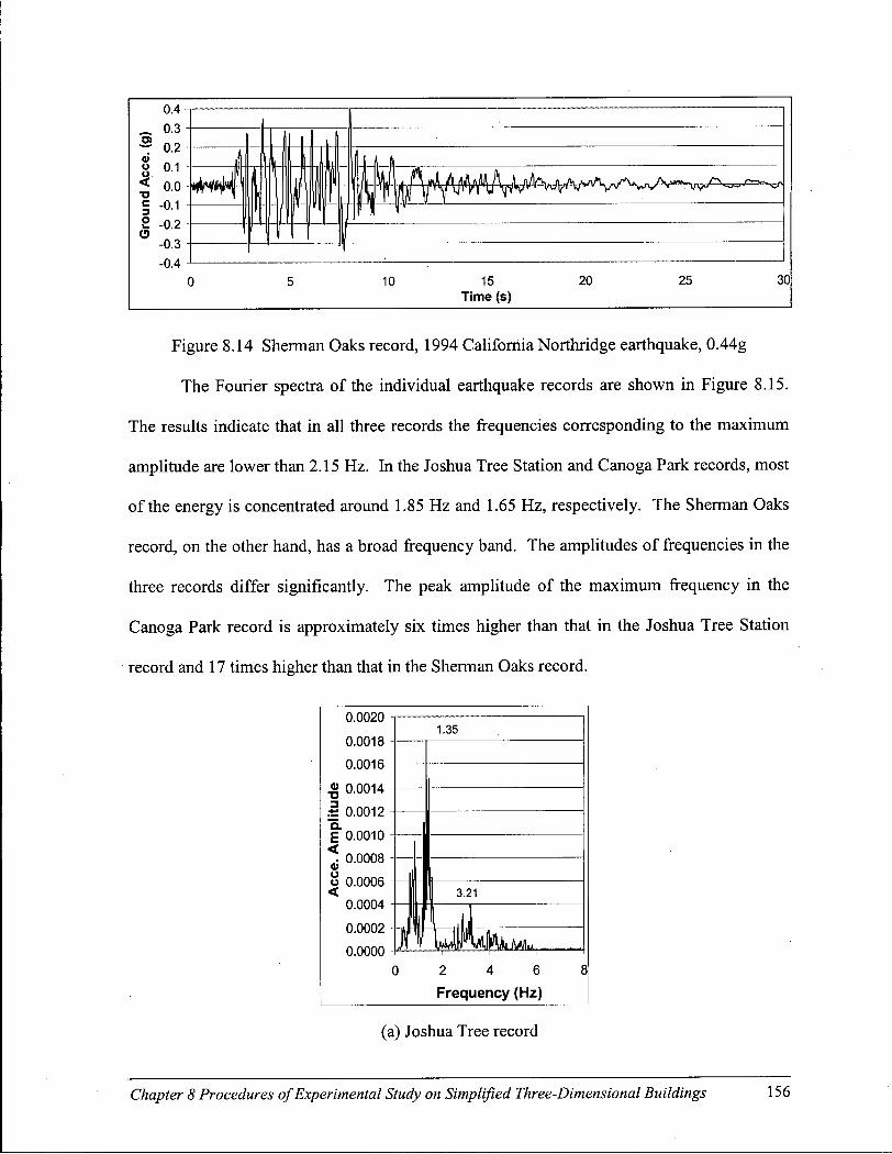
Figure 8.14 Sherman Oaks record, 1994 California Northridge earthquake, 0.44g
The Fourier spectra of the individual earthquake records are shown in Figure 8.15.
The results indicate that in all three records the frequencies corresponding to the maximum
amplitude are lower than 2.15 Hz. In the Joshua Tree Station and Canoga Park records, most
of the energy is concentrated around 1.85 Hz and 1.65 Hz, respectively. The Sherman Oaks
record, on the other hand, has a broad frequency band. The amplitudes of frequencies in the
three records differ significantly. The peak amplitude of the maximum frequency in the
Canoga Park record is approximately six times higher than that in the Joshua Tree Station
record and 17 times higher than that in the Sherman Oaks record.
0.0020
0.0018
0.0016
« 0.0014
| 0.0012
£ 0 . 0 0 1 0
^ 0.0008
o 0.0006
0.0004
0.0002
0.0000
1.35
3.21
iE2 2 4 6
Frequency (Hz)
(a) Joshua Tree record
Chapter 8 Procedures of Experimental Study on Simplified Three-Dimensional Buildings 156
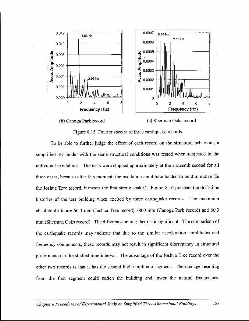
0.012
0.010
o •o 0.008
a E 0.006 < 6 o *\
0.004 <
0.002
0.000
1.63 Hz
ill ,2.98 Hz
i w 1 2 4 6
Frequency (Hz)
0.0007
0.0006
o 0.0005 3
"5. 0.0004 E < 0.0003 ai o u < 0.0002
0.0001
0.66 Hz
2.15 Hz
2 4 6 Frequency (Hz)
(b) Canoga Park record (c) Sherman Oaks record
Figure 8.15 Fourier spectra of three earthquake records
To be able to further judge the effect of each record on the structural behaviour, a
simplified 3D model with the same structural conditions was tested when subjected to the
individual excitations. The tests were stopped approximately at the sixteenth second for all
three cases, because after this moment, the excitation amplitude tended to be diminutive (In
the Joshua Tree record, it means the first strong shake.). Figure 8.16 presents the drift-time
histories of the test building when excited by three earthquake records. The maximum
absolute drifts are 66.3 mm (Joshua Tree record), 68.0 mm (Canoga Park record) and 60.3
mm (Sherman Oaks record). The difference among them is insignificant. The comparison of
the earthquake records may indicate that due to the similar acceleration amplitudes and
frequency components, these records may not result in significant discrepancy in structural
performance in the studied time interval. The advantage of the Joshua Tree record over the
other two records is that it has the second high amplitude segment. The damage resulting
from the first segment could soften the building and lower the natural frequencies.
Chapter 8 Procedures of Experimental Study on Simplified Three-Dimensional Buildings 157
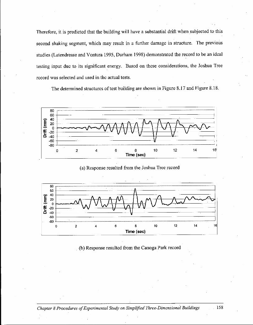
Therefore, it is predicted that the building will have a substantial drift when subjected to this
second shaking segment, which may result in a further damage in structure. The previous
studies (Latendresse and Ventura 1995, Durham 1998) demonstrated the record to be an ideal
testing input due to its significant energy. Based on these considerations, the Joshua Tree
record was selected and used in the actual tests.
The determined structures of test building are shown in Figure 8.17 and Figure 8.18.
80 60
0 2 4 6 8 10 12 14 16 Time (sec)
(a) Response resulted from the Joshua Tree record
80 T
-60 : ;
-80 -I : • : ' 0 2 4 6 8 10 12 14 16
Time (sec)
(b) Response resulted from the Canoga Park record
Chapter 8 Procedures of Experimental Study on Simplified Three-Dimensional Buildings 158
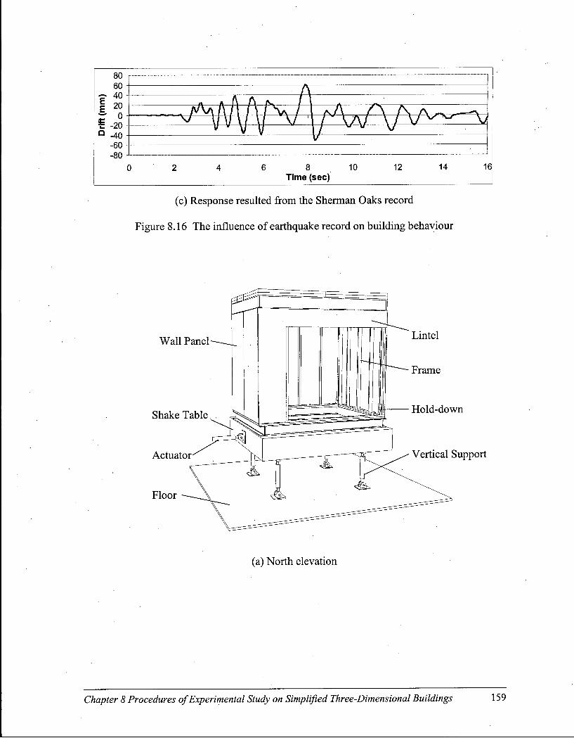
80 60
| 20
1 -20 Q -40
-60 -80
ft « ft A \ / 1 v \ \ \ \ \ / 1
v v v V
8 Time (sec)
10 12 14 16
(c) Response resulted from the Sherman Oaks record
Figure 8.16 The influence of earthquake record on building behaviour
Wall Panel
Shake Table
Actuator
Floor
Lintel
Frame
Hold-down
Vertical Support
(a) North elevation
Chapter 8 Procedures of Experimental Study on Simplified Three-Dimensional Buildings 159
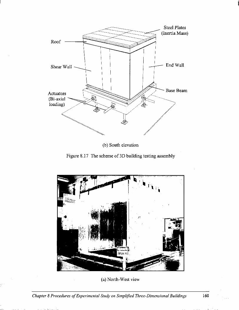
(b) South elevation
Figure 8.17 The scheme of 3D building testing assembly
(a) North-West view
Chapter 8 Procedures of Experimental Study on Simplified Three-Dimensional Buildings 160

(b) South-West view
Figure 8.18 The test building on shake table
The finite element programs were employed prior to testing to predict static and
dynamic response of the model buildings. Comparisons made after the tests were conducted
indicated that these predictions were in good agreement with the results obtained from
testing. The results will be described in Chapters 9 and 10 in detail.
8.3. Experimental procedures
A total of four three-dimensional building tests were carried out. In Test One, the
building was statically loaded, undergoing a monotonic pushover. No dead load was applied
to the building in this test. The test building in the second test was retrofitted from the first
test building by replacing all the panels on shear walls and re-installing all the hold-downs,
whereas the frame members were not changed (inspection showed no damage in frame
members). The steel plates as the dead load were attached to the roof of the test building.
The building was loaded statically in the same scheme as in the first test. In the static tests,
Chapter 8 Procedures of Experimental Study on Simplified Three-Dimensional Buildings 161

the shake table was moved to the west end to provide a 152 mm (6 in) lateral clearance. This
distance was believed to be enough for the test building to reach and go beyond the ultimate
strength level. The loading rate was 0.13 mm/sec in compliance with the tests done
previously at the U B C . The roof of test buildings was connected to the reaction column with
a rigid arm to remain stationary, whereas the base moved with the shake table. After the
second test, this building also served as the model to calibrate the Seismic Shock Simulation
System and the Data Acquisition System in regenerating the earthquake signals and
recording the test signals.
The third and fourth experiments were dynamic tests, with the Joshua Tree Station
records as the input excitation history. The specimen used in the third test was built with
four new walls. In the third test, the excitation was applied only in the x direction, whereas
in the fourth test, the building was subjected to a combination of earthquake components in
both the x and y directions. The specimen in the fourth test was retrofitted from that in the
third test, with all panels on four walls replaced. The sine wave frequency sweep tests were
conducted on both specimens, prior to the destructive earthquake excitations, to determine
the buildings' natural frequencies and corresponding mode shapes.
8.4. Brief description of the two-dimensional shear wall tests
In the last few years, a number of experimental projects have been carried out at the
University of British Columbia to investigate the structural performance of timber shear
walls. The database generated from the projects was capable of providing the required
information in the validation of the current numerical models.
Two types of the previously tested shear walls (Durham et al. 1997) were selected as
examples in this numerical study, which were tested under the both static loading and
Chapter 8 Procedures of Experimental Study on Simplified Three-Dimensional Buildings 162
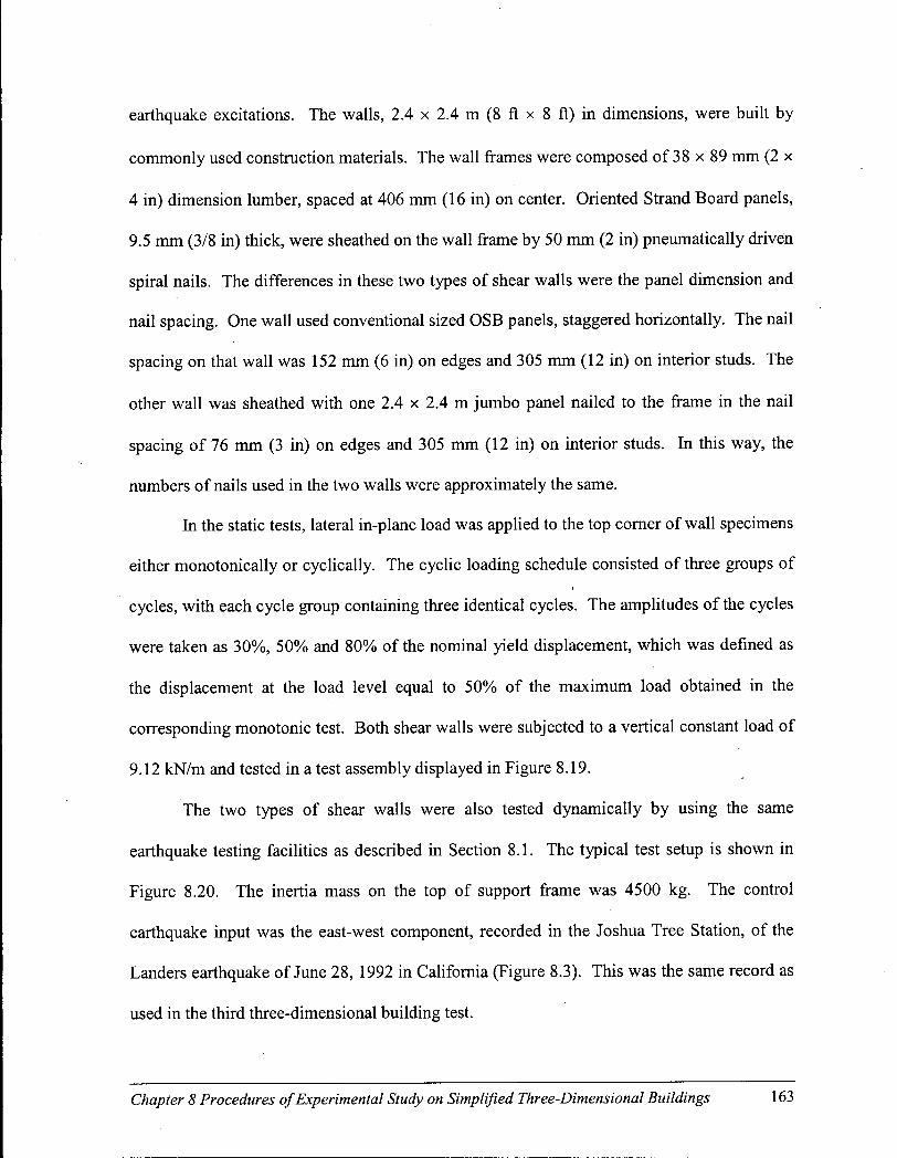
earthquake excitations. The walls, 2.4 x 2.4 m (8 ft x 8 ft) in dimensions, were built by
commonly used construction materials. The wall frames were composed of 38 x 89 mm (2 x
4 in) dimension lumber, spaced at 406 mm (16 in) on center. Oriented Strand Board panels,
9.5 mm (3/8 in) thick, were sheathed on the wall frame by 50 mm (2 in) pneumatically driven
spiral nails. The differences in these two types of shear walls were the panel dimension and
nail spacing. One wall used conventional sized OSB panels, staggered horizontally. The nail
spacing on that wall was 152 mm (6 in) on edges and 305 mm (12 in) on interior studs. The
other wall was sheathed with one 2.4 x 2.4 m jumbo panel nailed to the frame in the nail
spacing of 76 mm (3 in) on edges and 305 mm (12 in) on interior studs. In this way, the
numbers of nails used in the two walls were approximately the same.
In the static tests, lateral in-plane load was applied to the top corner of wall specimens
either monotonically or cyclically. The cyclic loading schedule consisted of three groups of
cycles, with each cycle group containing three identical cycles. The amplitudes of the cycles
were taken as 30%, 50% and 80% of the nominal yield displacement, which was defined as
the displacement at the load level equal to 50% of the maximum load obtained in the
corresponding monotonic test. Both shear walls were subjected to a vertical constant load of
9.12 kN/m and tested in a test assembly displayed in Figure 8.19.
The two types of shear walls were also tested dynamically by using the same
earthquake testing facilities as described in Section 8.1. The typical test setup is shown in
Figure 8.20. The inertia mass on the top of support frame was 4500 kg. The control
earthquake input was the east-west component, recorded in the Joshua Tree Station, of the
Landers earthquake of June 28, 1992 in California (Figure 8.3). This was the same record as
used in the third three-dimensional building test.
Chapter 8 Procedures of Experimental Study on Simplified Three-Dimensional Buildings 163
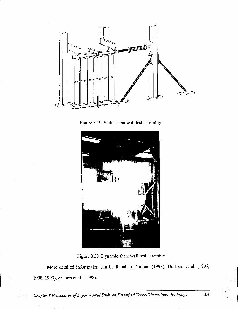
Figure 8.20 Dynamic shear wall test assembly
More detailed information can be found in Durham (1998), Durham et al. (1997,
1998, 1999), or Lam et al. (1998).
Chapter 8 Procedures of Experimental Study on Simplified Three-Dimensional Buildings

In this chapter, the test facilities and procedures are described in detail. The
experimental results will be presented in the next two chapters to better reflect the integrity
of the experimental based verification of the finite element models.
Chapter 8 Procedures of Experimental Study on Simplified Three-Dimensional Buildings 165

CHAPTER 9
EXPERIMENTAL-BASED VERIFICATION OF THE STATIC FINITE ELEMENT MODELS
The second stage of verification of the finite element models by using the
experimental data from the tests described in Chapter 8 is presented in this and the next
chapters. Although they were constructed as idealized models, the test buildings displayed
some of the behaviour found in the actual houses. Among those, the torsional effects,
deformations, and failure modes in the structural components were of much interest. The
finite element programs were operated mainly in the nonlinear range. This range was far
beyond the limitation of the verification presented in Chapter 7, which could only be
conducted for small deformations and in the linear elastic range. Therefore, the verification
described in these two chapters is much more meaningful and critical. Without such a step,
the verification of the finite element models would not be thorough and complete. Because
full size simplified test structures were used, this step can also be seen.as preliminary
application of the programs and study of wood light-frame building systems.
9.1. Experimental results of three-dimensional building under static loading conditions
Two three-dimensional buildings were tested under static unidirectional loading. The
following notations are defined to represent the characteristics of the test buildings obtained
from the tests, which are summarized in Table 9.1.
.Pmax = maximum load carrying capacity of test building, kN.
Chapter 9 Experimental-Based Verification of the Static Finite Element Models 166

A* = ultimate displacement of test building in x direction at the maximum
load P m a x , mm.
Ay = maximum displacement of test building in y direction, mm.
6 = maximum torsional rotation of the roof of test building about the
vertical axis, which passes through the center of mass of the roof diaphragm, rad.
D = dead load applied to test building, kN.
Oc\, ci = uplift displacements measured by dial gauges C l and C2, respectively,
mm. Referring to Figure 8.1, C l was located at the northeast corner of the building and C2
at the southeast corner of the building.
Table 9.1 Summary of static test results of three-dimensional buildings
Test No.
•Pmax (kN)
A , (mm)
A , (mm)
0 (rad)
Oci (mm)
Oci (mm)
D (kN)
1 28.3 96.6 11.3 1.04xl0"2 5.08 10.16 0.0
2 26.8 74.8 9.5 0.84xl0"2 4.57 9.14 71.1
The data from the two static tests were filtered before they could be implemented into
the analysis. Figure 9.1 provides the load-displacement relationship of the building in Test
One. The load reading was given by a load cell (Gl) installed in the rigid arm connecting to
the middle of the short span of the building roof, while the displacement was measured at the
shake table (DI). Figure 9.2 shows the load-displacement relationship of the building in Test
Two. It is notable that the load-displacement curves show a zigzag pattern, which indicate
cracking in the wood medium under the nail compression and failure in panels and frame
members.
Chapter 9 Experimental-Based Verification of the Static Finite Element Models 167
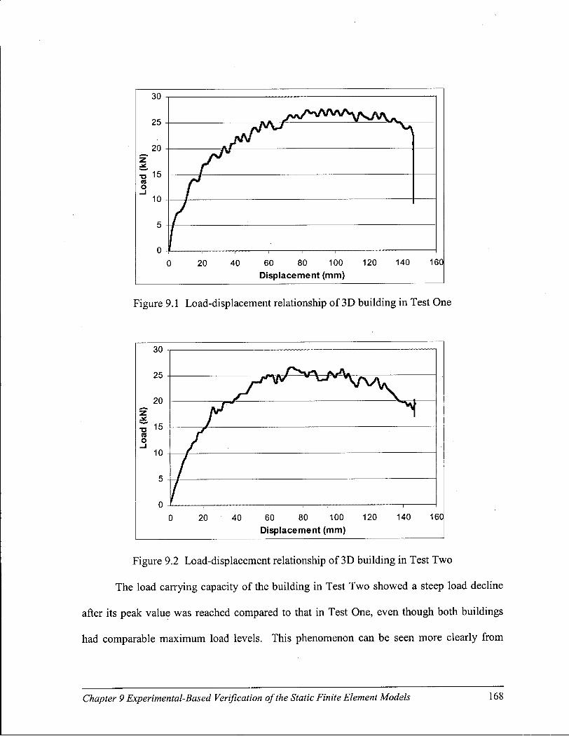
0 20 40 60 80 100 120 140 160 Displacement (mm)
Figure 9.1 Load-displacement relationship of 3D building in Test One
30
ra o 10 J—
7 • o I , , , , - ! , , 1
0 20 40 60 80 100 120 140 160
Displacement (mm)
Figure 9.2 Load-displacement relationship of 3D building in Test Two
The load carrying capacity of the building in Test Two showed a steep load decline
after its peak value was reached compared to that in Test One, even though both buildings
had comparable maximum load levels. This phenomenon can be seen more clearly from
Chapter 9 Experimental-Based Verification of the Static Finite Element Models

Figure 9.3 where two load-displacement curves are presented together. This can be
attributed to the P-A effect caused by the dead load applied to the second test building. The
dead load also resulted in smaller torsional motions and uplifts in the second building,
because the joints between frame members were firmly compressed downwards and,
therefore, resisted separation and rotation. For both tests, the uplift at the southeast corner
(C2) was greater than that at the northeast corner (Cl) . The reason was that the shear wall
without opening had a higher stiffness and therefore carried a higher load. The shear wall
with the opening was undergoing a larger overall lateral deformation, however.
30
25
20
15
10
5
0
Test One /
rf ' V Test Two
0 20 40 60 80 100 120 140 160]
Displacement (mm)
Figure 9.3 Comparison of load carrying capacities of two buildings
9.2. Prediction of behaviour of the three-dimensional buildings under static loading
conditions
The numerical predictions made by the LightFrame3D program on the maximum load
carrying capacities and the maximum torsional motions of the two test buildings are
compared with the static test results. Table 9.2 summarized these results, using the same
Chapter 9 Experimental-Based Verification of the Static Finite Element Models 169

definitions of notations as in Table 9.1. The numerical results from five points on the roof of
the building were recorded to calculate displacement and torsional motions. Among these
points, one was located at the center of the roof to measure the displacement in the x
direction, two respectively at the north and south corners in the x direction, and two
respectively at the east and west corners in the y direction. The difference in the
displacements measured at two opposite points (e.g. the north and south corners) was
calculated and then divided by the span of the roof to obtain the angle of roof rotation. The
rotational results in both x and y directions were similar, but not exactly the same due to
slight change in the roof geometric shape, because the roof was not perfectly rigid.
Table 9.2 Comparison of static test results and numerical predictions
Test Data max A* Ay 0 No. Source (kN) (mm) (mm) (rad)
1 Test 28.3 96.6 11.3 1.04xl0"2
LightFrame3D 27.9 90.0 6.3 0.31xl0"2
2 Test 26.8 74.8 9.5 0.84xl0"2
LightFrame3D 26.4 68.0 6.3 0.34xl0"2
The comparison between the numerical and experimental results indicates that the
finite element program can accurately predict the load-displacement characteristics of the
three-dimensional test buildings under static loading condition, as shown in Figure 9.4 for
Test One and Figure 9.5 for Test Two. The difference between the predicted and the tested
values in both cases was less than 4%. The predicted curves, including the initial stiffness,
closely matched the curves from the two tests.
Chapter 9 Experimental-Based Verification of the Static Finite Element Models 170

/£T Test
jf LightFrame3D
0 20 40 60 80 100 120 140 160
Displacement (mm)
Figure 9.4 Comparison of load-displacement characteristics in Test One
30
Displacement (mm)
Figure 9.5 Comparison of load-displacement characteristics in Test Two
The program predicted the torsional motion of the test buildings in the same pattern
as that shown in the tests. Figure 9.6 displays the roof deformation values in both the x and y
directions obtained from the prediction to the building in Test One.
Chapter 9 Experimental-Based Verification of the Static Finite Element Models 171

ROOF DEFORMATION (mm)
2.51
2.5
80.1 80.1 80.0__
r " l . 7 _ " \ \
85.0j DEFORMATION LINE
2.1 3.0 80.0 ~\
80.0 80.0
3.01 85.0
I 90.0 ' 2.5
LOADING DIRECTION 3 1
8 9 7
89.2 3.1|
_89JJ 2.5
87.5 87.5 87
2:51
2.2 3.11 6 87.6_ _ ] - - - - - " [
* 8 7 ^ 8 7 7 1.7 '
Figure 9.6 Plan view of the displaced position of the top of the test building
The resultant torsional motion is shown on the displaced diaphragm, illustrated by the
dashed lines. The roof experienced a combination of translational and rotational
deformations. The four walls slightly deformed out-of-plane because of the uneven out-of-
plane and in plane displacements as well as different drift values. In the x direction, the north
shear wall was subject to more severe deformation than the south shear wall due to the larger
opening and accordingly, in the y direction the east end wall moved towards the north while
the west end wall moved towards the south. The curved deformations in both the transverse
end walls indicate that the roof in the model was not completely rigid.
The comparisons of torsional motions of test buildings presented in Table 9.2 indicate
that the predicted torsional motions in both buildings were considerably smaller. This
consequence can be partially attributed to the connection model used in the frame element,
which required four three-dimensional beam elements in a frame element to be rigidly
connected. In an actual wood frame building, however, the frame members would usually be
Chapter 9 Experimental-Based Verification of the Static Finite Element Models 172
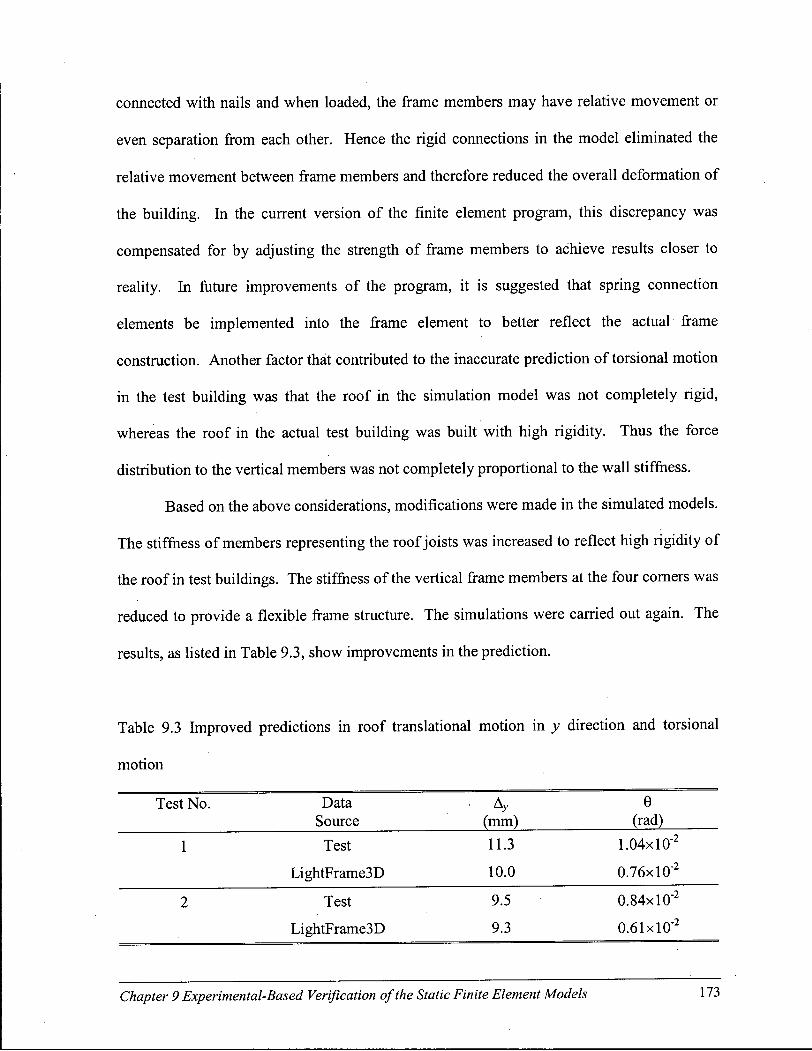
connected with nails and when loaded, the frame members may have relative movement or
even separation from each other. Hence the rigid connections in the model eliminated the
relative movement between frame members and therefore reduced the overall deformation of
the building. In the current version of the finite element program, this discrepancy was
compensated for by adjusting the strength of frame members to achieve results closer to
reality. In future improvements of the program, it is suggested that spring connection
elements be implemented into the frame element to better reflect the actual frame
construction. Another factor that contributed to the inaccurate prediction of torsional motion
in the test building was that the roof in the simulation model was not completely rigid,
whereas the roof in the actual test building was built with high rigidity. Thus the force
distribution to the vertical members was not completely proportional to the wall stiffness.
Based on the above considerations, modifications were made in the simulated models.
The stiffness of members representing the roof joists was increased to reflect high rigidity of
the roof in test buildings. The stiffness of the vertical frame members at the four corners was
reduced to provide a flexible frame structure. The simulations were carried out again. The
results, as listed in Table 9.3, show improvements in the prediction.
Table 9.3 Improved predictions in roof translational motion in y direction and torsional
motion
Test No. Data • A, 0 Source (mm) (rad)
1 Test 11.3 1.04xl0"2
LightFrame3D 10.0 0.76xl0"2
2 Test 9.5 0.84x10"2
LightFrame3D 9.3 0.61 xlO" 2
Chapter 9 Experimental-Based Verification of the Static Finite Element Models 173

During the simulation procedures, it was thought that even i f a better prediction to an
individual test case could be achieved by selecting more carefully calibrated parameters, it is
more important for a researcher to focus on building a robust analytical tool that not only can
simulate some specified cases, but also can successfully predict structures with a wide range
of combinations of material and loading conditions. In testing the finite element program's
capacity, the behaviour of a building subject to a post-peak cyclic loading was predicted, as
shown in Figure 9.7. This example demonstrates the advantage of the computer simulation
over the testing method in terms of cost and time effectiveness. It also indicates that without
performing an actual laboratory test, a structure can be investigated by using different
parameters, as in a parameter study.
40
30
20
Z 10
•a 0 n o -I -10
-20
-30
40
30
20
Z 10
•a 0 n o -I -10
-20
-30
40
30
20
Z 10
•a 0 n o -I -10
-20
-30
40
30
20
Z 10
•a 0 n o -I -10
-20
-30
40
30
20
Z 10
•a 0 n o -I -10
-20
-30
40
30
20
Z 10
•a 0 n o -I -10
-20
-30
40
30
20
Z 10
•a 0 n o -I -10
-20
-30
40
30
20
Z 10
•a 0 n o -I -10
-20
-30
40
30
20
Z 10
•a 0 n o -I -10
-20
-30 - tu
-160 -120 -80 -40 0 40 80 120 160
Displacement (mm)
Figure 9.7 Predicted post-peak cyclic load-displacement behaviour of building in Test One
(with static back bone curves)
9.3. System effects
It is generally agreed that a structural component will behave differently depending
upon whether it is used in a building system or loaded on its own. This is because the system
Chapter 9 Experimental-Based Verification of the Static Finite Element Models 174

effects, including load sharing among components, deformation reassignment, and system
eccentricity, will affect the actual forces and deformations in each individual building
component. The degree of system effects depends mainly on the material, geometric, and
structural layout of a building. For example, an asymmetric arrangement of openings may
generate an uneven distribution of forces in walls, which will cause torsion in the building.
The system effects, however, cannot be detected in two-dimensional component studies. To
reveal the system effects, a preliminary study was performed. From the numerical results
simulating the building in Test One, the forces applied to frame members at floor level are
presented in Figure 9.8.
F O R C E S APPLIED AT F L O O R L E V E L (kN) (NOT INCLUDE F O R C E S L E S S T H A N 0.2 kN)
18.2
6.0 •
4.2_
0.9N
^3.3 2 9 , | / ^ X o ,
3.3„
^ Z 5
1.6
o.sJ 3.2,
1.7
X 0.4s-
19.8
0.4 0.5
0.8^X. 1.7 15.1
0.9̂
1.1
1.3
2.1
0.4
0.8 2.5
o.exL^10
Figure 9.8 Forces in frame members measured at floor level
Figure 9.8 shows that the south shear wall (no opening) carried most of the lateral
load applied in the x direction (loading direction) because of its high stiffness. Sharing the
corner frame members resulted in notable lateral forces in the direction perpendicular to
Chapter 9 Experimental-Based Verification of the Static Finite Element Models 175
loading direction (the y direction) in the frame members of two end walls, even though no
external lateral load was applied on them in that direction. In the finite element models, the
two adjacent walls are connected by assuming that the end studs in the frames of two walls
are sharing a pair of common nodes.
To study the influence of system effect on the deflections of shear walls, the two
shear walls (the south and north shear walls) were loaded individually. The deflection results
were then compared to those when the two shear walls were integrated into a three-
dimensional building system, as the one in the tests. The results, given in Table 9.4, show
that the deflections of a shear wall in a system or loaded individually are substantially
different, which indicates that the appearance of transverse end walls and roof played roles in
adjusting the deformations in shear walls. This phenomenon reveals an important fact that
the system effect or load sharing mechanism can virtually redistribute the stiffness of
components to prevent the weakest one from undergoing excessive deformation, which
implies that the total deformation and load carrying capacity of a system are not simple
addition of those possessed by individual structural components in the system. This may also
explain the reason why some buildings with wide openings could survive in a severe
earthquake ground motion.
Table 9.4 Comparison of the deflection of shear walls with and without system effect
Deflection at P, n a x (mm) South shear wall (No opening) North shear wall (Opening)
Shear walls in 3D 80.0 87.6 building
80.0
Shear walls loaded 68.0 122.0 individually
68.0
It is worth mentioning that the corner studs picked up higher vertical forces than did
Chapter 9 Experimental-Based Verification of the Static Finite Element Models 176
the intermediate studs, as shown in Figure 9.8. A higher tensile force in the southeast corner
stud than that in the northeast one corroborates the results given in Table 9.1 that the
southeast corner stud had a larger uplift than the northeast one (Oci vs. Oci). In the current
version of the programs, it is not possible to quantitatively predict the uplift values. In order
for the program to do so, spring elements containing the same load-deformation
characteristics as the hold-downs have to be implemented in between the frame nodes and
supports. This can be done when the further improvement of the programs is performed.
9.4. Failure modes and relative movement between panel and frame
As discussed earlier, the shear walls in a wood light-frame system are major load-
carrying components. Under lateral loading, the overall performance of the shear wall
mostly depends on qualities of the sheathing panels and the connections attaching the panels
to framing members because the framing on its own has little lateral load carrying capacity.
The panels typically behave as relatively stiff plates, whereas the sheathing-framing
connections typically undergo highly nonlinear inelastic deformations. Surveys of previous
experimental studies and damaged wood frame buildings demonstrate the importance of the
nail connection between panels and frame members because the predominant failure mode
almost always involved the above-mentioned connection.
In the present static tests, failure was also first observed starting from the nail
connections holding the panels to the frame members. This nail connection failure was
mostly located around the edges of sheathing panels. It can be seen that initially the nails
bent and crushed into the frame members when relative movement between panel and frame
occurred. Along with the panel rotating with respect to or separating from the frame, the nail
gradually withdrew from the frame members (Figure 9.9 (a)). As the deformation
Chapter 9 Experimental-Based Verification of the Static Finite Element Models 177

progressed, failure in the form of nail heads embedding into and pulling through the panels
was observed (Figure 9.9 (b)). The tests indicated that the latter failure mode was more
influential because the panel could no longer play any structural role once its connection to
the frame was broken.
(a) Nail withdrawal from frame member (b) Nail pulling though the panel
Figure 9.9 Failure modes of nail connections
The finite element program predicted that the maximum nail forces would first occur
along the bottom panel edges of the shear wall without opening (the south wall) in the early
stage of loading and then progressed along the vertical panel edges of the same wall upwards.
In the end of simulation, the maximum nail forces were mainly located in the top panel
edges. This shift in the maximum nail forces implied a trend of the failure in nail
connections from the bottom to the top of the shear wall, which was the same as observed in
the tests.
Along with the increasing load and propagating nail failure, the sheathing panels
gradually rotated relative to the frame and, at some locations, separated from the frame. The
panels on the north shear wall (with opening) and the south shear wall (without opening)
stopped in positions as shown in Figure 9.10 and Figure 9.11, respectively. As a comparison,
Chapter 9 Experimental-Based Verification of the Static Finite Element Models 178

the panel positions predicted by LightFrame3D program are presented in Figure 9.12 for the
north shear wall and in Figure 9.13 for the south shear wall, respectively. A good agreement
was achieved between the tests and the simulations. Contrary to considerable damage
observed in the two side shear walls, the panels on both end walls did not display any
apparent damage or significant movement. It was because those walls underwent only slight
deformation and most of it was recovered after the load removal.
Figure 9.10 Panel movements of the north shear wall
(a) Top (Panel perimeters are highlighted)
Chapter 9 Experimental-Based Verification of the Static Finite Element Models 179
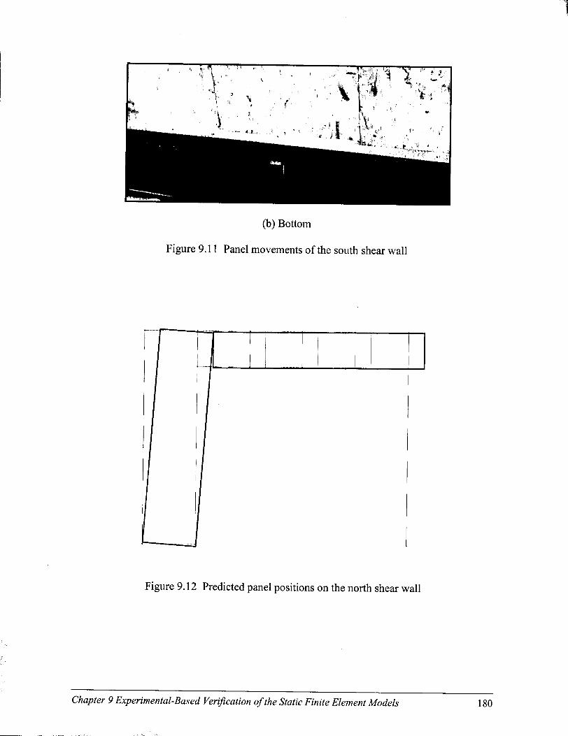
(b) Bottom
Figure 9.11 Panel movements of the south shear wall
Figure 9.12 Predicted panel positions on the north shear wall
Chapter 9 Experimental-Based Verification of the Static Finite Element Models 180
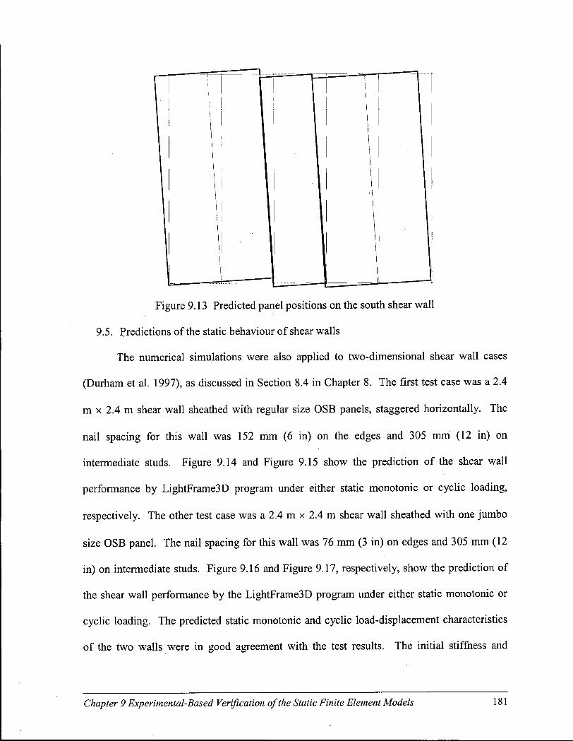
Figure 9.13 Predicted panel positions on the south shear wall
9.5. Predictions of the static behaviour of shear walls
The numerical simulations were also applied to two-dimensional shear wall cases
(Durham et al. 1997), as discussed in Section 8.4 in Chapter 8. The first test case was a 2.4
m x 2.4 m shear wall sheathed with regular size OSB panels, staggered horizontally. The
nail spacing for this wall was 152 mm (6 in) on the edges and 305 mm (12 in) on
intermediate studs. Figure 9.14 and Figure 9.15 show the prediction of the shear wall
performance by LightFrame3D program under either static monotonic or cyclic loading,
respectively. The other test case was a 2.4 m x 2.4 m shear wall sheathed with one jumbo
size OSB panel. The nail spacing for this wall was 76 mm (3 in) on edges and 305 mm (12
in) on intermediate studs. Figure 9.16 and Figure 9.17, respectively, show the prediction of
the shear wall performance by the LightFrame3D program under either static monotonic or
cyclic loading. The predicted static monotonic and cyclic load-displacement characteristics
of the two walls were in good agreement with the test results. The initial stiffness and
Chapter 9 Experimental-Based Verification of the Static Finite Element Models 181
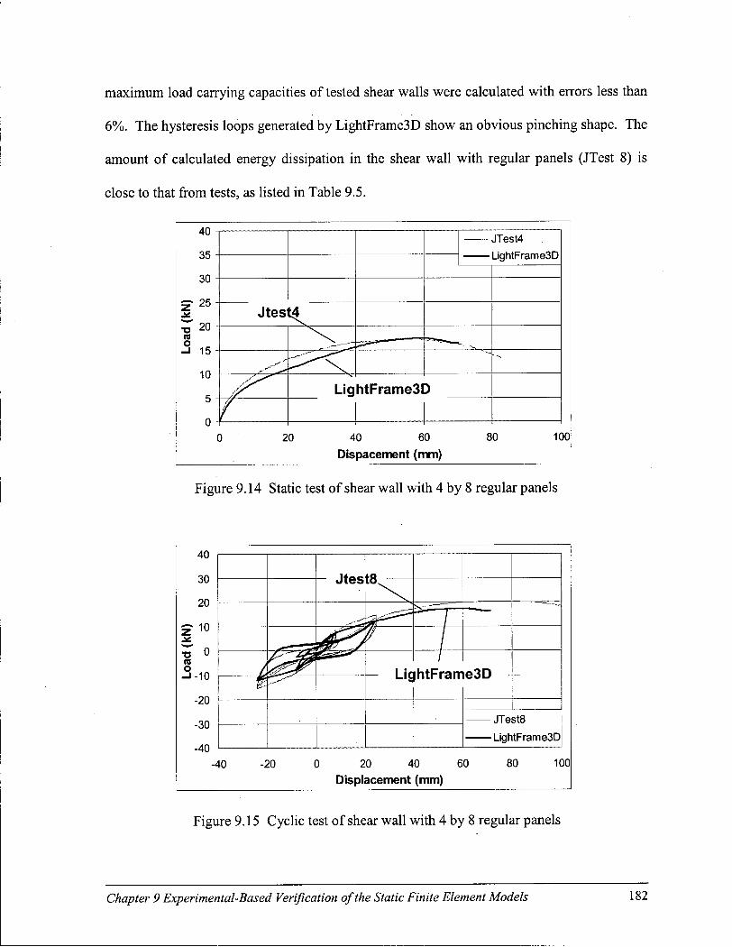
maximum load carrying capacities of tested shear walls were calculated with errors less than
6%. The hysteresis loops generated by LightFrame3D show an obvious pinching shape. The
amount of calculated energy dissipation in the shear wall with regular panels (JTest 8) is
close to that from tests, as listed in Table 9.5.
JTest4 LightFrame3D JTest4 LightFrame3D
Jtest4
— — *
X \ Lig htFrame3D
0 20 40 60 80 100 Dispacement (mm)
Figure 9.14 Static test of shear wall with 4 by 8 regular panels
40
30
20
z 1 0
•o 0 re o -1 -10
-20
-30
-40
1
lO
" /
Lir /
ihtFrarr I G3D
/ ihtFrarr
JTest8 LightFrame3D JTest8 LightFrame3D
-40 -20 0 20 40 Displacement (mm)
60 80 100
Figure 9.15 Cyclic test of shear wall with 4 by 8 regular panels
Chapter 9 Experimental-Based Verification of the Static Finite Element Models 182

40
35
30
z 25
T3 20 ra o _ l 15
10
5
0
f 1 JghtFrarm -3D / _̂
/ I JghtFrarm -3D Jtest3
/ JTest3 LightFrame3D JTest3 LightFrame3D
20 40 60 Displacement (mm)
80 100
Figure 9.16 Static test of shear wall with one jumbo panel
40
30
20
z 10 JL ~o 0 ra o _i -10
-20
-30
-40
/_ Jtest6
4 LightFrame3D
(// w HAS
JTest6
LightFrame3D
-40 -20 0 20 40 60 Displacement (mm)
80 100
Figure 9.17 Cyclic test of shear wall with one jumbo panel
Table 9.5 Comparison of energy dissipation of shear walls under cyclic loading predicted by
LightFrame3D program and measured from tests
Shear Wall Energy Dissi pation (N-m) Error (%)a Shear Wall Test LighfFrame3D
JTest 6 - 2.4x2.4 Jumbo Panel JTest 8 - 1.2x2.4 Regular Panels
3378 1081
2630 1038
28 4
a : E r r o r = Ana.-Test x l Q Q
Ana.
Chapter 9 Experimental-Based Verification of the Static Finite Element Models 183
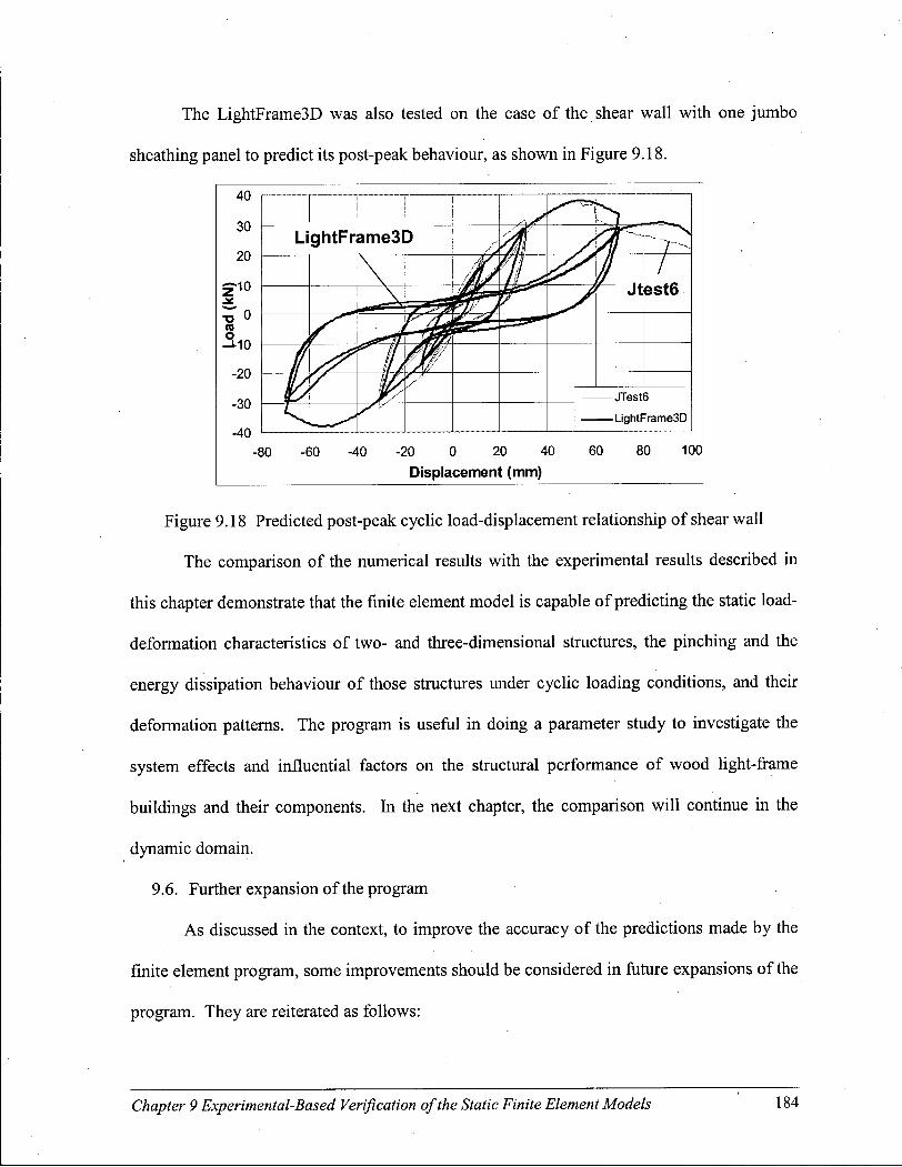
The LightFrame3D was also tested on the case of the shear wall with one jumbo
sheathing panel to predict its post-peak behaviour, as shown in Figure 9.18.
40 30 20
z 1 0
* o ra o
—1-10
-20 -30 -40
LightFrame3D
est6 (rJr\ I w * ^ ' j t est6
JTest6
LightFrame3D
JTest6
LightFrame3D
-80 -60 -40 -20 0 20 40 Displacement (mm)
60 80 100
Figure 9.18 Predicted post-peak cyclic load-displacement relationship of shear wall
The comparison of the numerical results with the experimental results described in
this chapter demonstrate that the finite element model is capable of predicting the static load-
deformation characteristics of two- and three-dimensional structures, the pinching and the
energy dissipation behaviour of those structures under cyclic loading conditions, and their
deformation patterns. The program is useful in doing a parameter study to investigate the
system effects and influential factors on the structural performance of wood light-frame
buildings and their components. In the next chapter, the comparison wil l continue in the
dynamic domain.
9.6. Further expansion of the program
As discussed in the context, to improve the accuracy of the predictions made by the
finite element program, some improvements should be considered in future expansions of the
program. They are reiterated as follows:
Chapter 9 Experimental-Based Verification of the Static Finite Element Models 184

(1) To better reflect the actual frame construction, the rigid connection of frame elements
needs to be changed to a flexible connection, which can be done by implementing
spring elements in the connections of frame elements;
(2) Spring elements representing the actual material properties of the hold-downs can be
added to the frame nodes connecting the support foundation to predict the uplift in the
structure under varied loading schemes.
Chapter 9 Experimental-Based Verification of the Static Finite Element Models 185

CHAPTER 1 0
EXPERIMENTAL-BASED VERIFICATION OF THE DYNAMIC FINITE ELEMENT MODELS
As the continuation of the experimental-based verification of the finite element
models, this chapter focuses on comparing the dynamic response of three-dimensional and
two-dimensional structures obtained from experimental procedures and numerical analyses.
In this chapter, first the test data are presented, followed by the predictions from the
LightFrame3D dynamic finite element program, which are then compared to the test results.
The natural frequencies and corresponding mode shapes, nonlinear dynamic characteristics,
and the failure modes of test systems from both resources are subsequently discussed. Test
Four is also described in this chapter in detail, even though the present program is not
capable of providing predictions to it.
The raw data from the dynamic tests contained high frequency noise components
generated from the electronic apparatus in the test control and signal generation systems.
The noise had to be eliminated before the test data could be implemented into the analysis.
This is usually accomplished using digital data processing techniques, in which the central
step is the Fast Fourier Transform (FFT). The descriptions of the theory and methods in
digital data processing can be found in a number of publications, including the books written
by Bendat and Piersol (1986) and Newland (1986). In the present testing, an integral data
processing routine in both time domain and frequency domain was applied. In the time
Chapter 10 Experimental-Based Verification of the Dynamic Finite Element Models 186
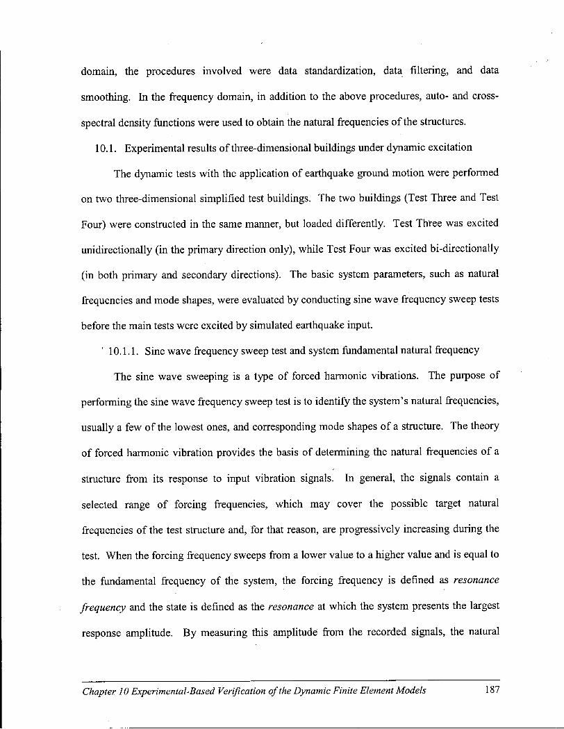
domain, the procedures involved were data standardization, data filtering, and data
smoothing. In the frequency domain, in addition to the above procedures, auto- and cross-
spectral density functions were used to obtain the natural frequencies of the structures.
10.1. Experimental results of three-dimensional buildings under dynamic excitation
The dynamic tests with the application of earthquake ground motion were performed
on two three-dimensional simplified test buildings. The two buildings (Test Three and Test
Four) were constructed in the same manner, but loaded differently. Test Three was excited
unidirectionally (in the primary direction only), while Test Four was excited bi-directionally
(in both primary and secondary directions). The basic system parameters, such as natural
frequencies and mode shapes, were evaluated by conducting sine wave frequency sweep tests
before the main tests were excited by simulated earthquake input.
10.1.1. Sine wave frequency sweep test and system fundamental natural frequency
The sine wave sweeping is a type of forced harmonic vibrations. The purpose of
performing the sine wave frequency sweep test is to identify the system's natural frequencies,
usually a few of the lowest ones, and corresponding mode shapes of a structure. The theory
of forced harmonic vibration provides the basis of determining the natural frequencies of a
structure from its response to input vibration signals. In general, the signals contain a
selected range of forcing frequencies, which may cover the possible target natural
frequencies of the test structure and, for that reason, are progressively increasing during the
test. When the forcing frequency sweeps from a lower value to a higher value and is equal to
the fundamental frequency of the system, the forcing frequency is defined as resonance
frequency and the state is defined as the resonance at which the system presents the largest
response amplitude. By measuring this amplitude from the recorded signals, the natural
Chapter 10 Experimental-Based Verification of the Dynamic Finite Element Models 187
frequency of the system can be determined and the associated damping can be subsequently
calculated. Theoretically, the resonance frequency is slightly different for displacement,
velocity, and acceleration, which, for a damped system, can be described as:
Displacement resonance frequency = co-v/l - 2C2
Velocity resonance frequency = co
Acceleration resonance frequency = co/-\\-2C1
The differences among the three resonance frequencies and the natural frequency are
negligible because the damping in a typical wood structure is well below the 20%, at which a
maximum 4% error is introduced. In the present tests, all system natural frequencies were
determined from the acceleration signals. The obtained results would be slightly larger than
the true natural frequency, but the error was insignificant.
The sine wave sweep tests performed prior to the main earthquake tests in Tests Three
and Four included three forcing frequency ranges to cover the three possible lowest natural
frequencies and mode shapes, representing the two translational motions and the one
rotational motion. With the help of the LightFrame_Eigen program, the three selected ranges
were 0.5 Hz - 6.0 Hz, 4.0 Hz - 10.0 Hz, and 7.0 Hz - 15.0 Hz. During the tests, the sweeps
were at constant displacement with amplitude of 0.5 mm. In determining the natural
frequencies, FFT analysis was applied to the acceleration signals taken from four
accelerometers positioned at three corners and at the center of the top of the test buildings. In
each range, the resultant frequency values from the FFT analysis were averaged to provide
the final natural frequency. The differences among all the measurements were minor. In
determining the mode shapes, the phases and amplitudes of the acceleration signals obtained
from different locations were compared. In the first sine sweep frequency range (0.5 Hz -
Chapter 10 Experimental-Based Verification of the Dynamic Finite Element Models 188

6.0 Hz), the translational motions measured at the two corners (E2 and E3) on the roof had
the same phase in the primary direction (Figure 10.1). The amplitude in the primary
direction was significantly higher than that in the secondary direction (El) (Figure 10.2).
The rotation of the roof was not significant when comparing the phases of signals obtained
from the two corners on the roof (E3 and E4) as shown in Figure 10.3. These results
demonstrated that the mode shape under the first sine sweep excitation was the first mode
shape corresponding to the first natural frequency of the test structure. In the second sine
sweep frequency range (4.0 Hz - 10.0 Hz), the acceleration waves measured at E3 and E4 in
the secondary direction were in the same phase (Figure 10.4). The amplitude in the
secondary direction measured at the center of the roof was much higher than that in the
primary direction measured at the same location, as shown in Figure 10.5. It was the same as
in the first frequency range that the rotation of the roof was not significant when comparing
the signals measured at the two opposite corners (Figure 10.6). From these results, it is
concluded that the structure was undergoing the translational motion in the secondary
direction with the second mode shape corresponding to the second natural frequency. In the
third sine sweep frequency range, the acceleration signals measured at the opposite corners
(E2 vs. E3 and E3 vs. E4) in both directions were in the reverse phases (Figure 10.7 and
Figure 10.8). This phenomenon indicated that the structure was subject to a rotational
motion (The third mode shape) corresponding to the third natural frequency.
Chapter 10 Experimental-Based Verification of the Dynamic Finite Element Models 189

Figure 10.1 Amplitudes in the primary direction in the first frequency range
Figure 10.2 Amplitudes in two directions in the first frequency range
Figure 10.3 Comparison of the phases of two signals in the first frequency range
Chapter JO Experimental-Based Verification of the Dynamic Finite Element Models 190

Time (sec)
Figure 10.4 Amplitudes in the secondary direction in the second frequency range
13 14 15 16 17 18 19 20 Time (sec)
Figure 10.5 Amplitudes in two directions in the second frequency range
< -0.02 J •••
13 14 15 16 17 18 19 20 Time (sec)
Figure 10.6 Comparison of the phases of two signals in the second frequency range
Chapter 10 Experimental-Based Verification of the Dynamic Finite Element Models 191

8 -oi
-0.2 '
17.0 17.5 18.0 18.5 19.0
Time (sec)
Figure 10.7 Phases of two signals in the primary direction in the third frequency range
17.0 17.5 18.0 18.5 19.0
Time (sec)
Figure 10.8 Phases of two signals in the secondary direction in the third frequency range
The natural frequencies and matching mode shapes for two tests are summarized in
Table 10.1. Three natural frequencies of Test Building Three are combined in Figure 10.9,
and those for Test Building Four are in Figure 10.10. These results show that the
fundamental natural frequencies are not well separated. During the data processing, this
incidence was observed. The building in Test Four provided lower natural frequency values
than those in Test Three. The reason for this may be due to the use of a retrofitted test
building in Test Four, in which the sheathing on all four walls from Test Three was replaced
with new panels but the original frame members were reused.
Chapter 10 Experimental-Based Verification of the Dynamic Finite Element Models 192
Table 10.1 Natural frequencies obtained from sine wave sweep tests
Mode Shape Test Three (f, Hz) Test Four (f4, Hz) A=(/3-/ 4)//3 (%)
First (Translation in x) 2.9 2.5 13.8
Second (Translation iny) 5.1 3.8 25.5
Third (Rotation about z) 8.8 8.2 6.8
1.2
•g 1.0 3
I 0 8
D 0.6 O N 5 0.4
2 0.2
0.0
1st, 2.9 Hz 2nd, 5.1Hz 3rd, 8.8 Hz
\ \ \ J
6 8 Frequency(Hz)
10 12 14
Figure 10.9 Three natural frequencies of building in Test Three
1.2
•o 1.0 3
a E
0.8
< T3
0.6 0) .a 1 0.4
o z 0.2
0.0
1st, 2.5 Hz 2nd, 3.8 Hz 3rd, 8.2 Hz
^ ^ 1 J \ 1 V. \ h '1 /•
6 8 Frequency (Hz)
10 12 14
Figure 10.10 Three natural frequencies of building in Test Four
10.1.2. Input acceleration signals
In the two dynamic tests, the earthquake waves in The 1992 Landers, California,
recorded at the Joshua Tree Station were used as the input excitations to the structures. In
Chapter 10 Experimental-Based Verification of the Dynamic Finite Element Models 193
Test Three, the building was excited unidirectionally in the long span with the east-west
acceleration component of the earthquake, and the peak acceleration of the record was scaled
up to a target value of 0.35g. In Test Four, the building was excited bi-directionally in both
the long and short spans. The east-west acceleration component of the earthquake was
applied to the long span, and the north-south component was applied to the short span. The
target peak acceleration was 0.29g, using the original records without scaling. The reason for
using lowered acceleration amplitude in this test was because in Test Three, the building was
subjected to very severe damages in the first pulse of the excitation and lost most of its lateral
load carrying capacity before the second pulse. Therefore, the purpose of investigating the
influence of two pulses on the structural behaviour was not accomplished.
In the tests, the actual peak accelerations of input signals were slightly different from
the target levels, due to accuracy limits in the signal generation apparatus and the electrical
noise introduced in the testing system. To examine i f the shake table can accurately
reproduce the input ground motion without losing acceleration frequency components, a 5%
damped acceleration response spectrum analysis was conducted. From the 5% damped
pseudo-acceleration response spectra (Figure 10.11), it is found that the frequency
components in the input acceleration signal and the shake table feedback in the entire range
were basically the same.
Chapter 10 Experimental-Based Verification of the Dynamic Finite Element Models 194
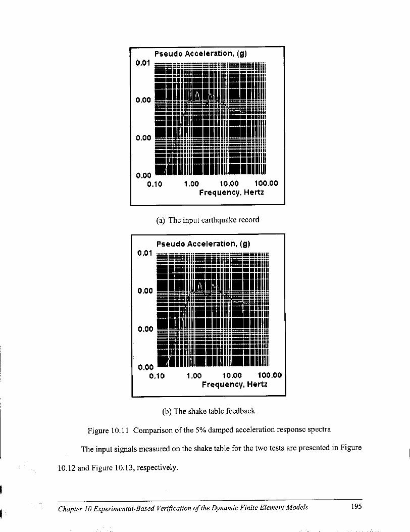
Pseudo Acceleration, (g) 0.01 WMMMHSMMIMMSMSSKMJMMHSSS
• • • • • l i • • • • • • • • I I I
• • I I I W B 1 I I I I I • • • I I I I M H B I I I I • i m i m a i i i i i i
0.00
0.00 S S
• • • ' J I M M H I I I I I I JIIIHHIIIIII
0.00
• • l i n n • I
• • • l l l l • • m i l !
m i n • m i n i I.HIIHB mm n i . a i m ...... !• — • »•»»»!•«
J B I I I I M a a iiiiiiiassiiii;:i mm! •mm i
• • • • • • l l l l
• • • • •un • • •min
0.10 1.00 10.00 100.00 Frequency, Hertz
(a) The input earthquake record
Pseudo Acceleration, (g)
o.oo SI!!!!!
0.00
0 00 ~ " ' " - M ! ! ™ ! 5 5 5 ! V . W m/mmmmmwmt&mmwitm • • — — mm mm m
0.10 1.00 10.00 100.00 Frequency, Hertz
(b) The shake table feedback
Figure 10.11 Comparison of the 5% damped acceleration response spectra
The input signals measured on the shake table for the two tests are presented in Figure
10.12 and Figure 10.13, respectively.
Chapter 10 Experimental-Based Verification of the Dynamic Finite Element Models 195
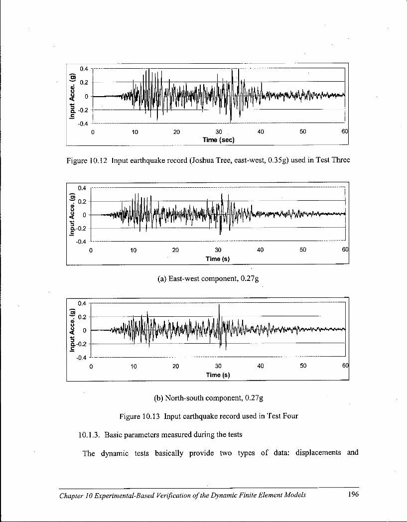
Figure 10.12 Input earthquake record (Joshua Tree, east-west, 0.35g) used in Test Three
(a) East-west component, 0.27g
(b) North-south component, 0.27g
Figure 10.13 Input earthquake record used in Test Four
10.1.3. Basic parameters measured during the tests
The dynamic tests basically provide two types of data: displacements and
Chapter 10 Experimental-Based Verification of the Dynamic Finite Element Models 196

accelerations. These data are recorded as absolute values. In order to extract the building
characteristics of deformations, forces, and failure modes, appropriate processing and
analysis of the saved data sets are necessary. The building deformations are described by
three degrees of freedom defined at the center of mass of the roof. They are the two lateral
displacements in the x and y directions and the one torsional rotation about the vertical axis.
The actual lateral building deformation (relative displacement or drift) is defined as the
difference between the total displacement of the mass of the roof and the displacement of the
ground (shake table). The actual (relative) mass acceleration comes from the same concept
as that for the relative displacement. To define the forces applied to test buildings, the
general equations of motion presented in Chapter 6 are described again:
ma, + ca + fs(a,a)-R = 0 (10.1)
Because
a, = a + a, (10.2)
By changing the order, the general equations of motion (10.1) can be presented as
ma + ca + fs(a,a) = R-ma g =R-P e # (10.3)
The last term Pe_#-(R are dead loads) on the right-hand side of Equation (10.3) represent the
external lateral forces applied to building induced from the earthquake, which are equal to
mass multiplied by the ground acceleration and acts opposite to the acceleration. These
forces are called the effective earthquake forces. The usefulness of this definition is that the
base shear, an essential parameter required in design procedures, can be calculated from the
effective earthquake forces. When only one storey is present, the effective earthquake force
equals the base shear. Based on this definition, when the same earthquake input
accelerogram and mass are applied to the test building and numerical model, the effective
Chapter 10 Experimental-Based Verification of the Dynamic Finite Element Models 197
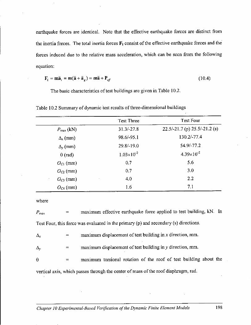
earthquake forces are identical. Note that the effective earthquake forces are distinct from
the inertia forces. The total inertia forces Fi consist of the effective earthquake forces and the
forces induced due to the relative mass acceleration, which can be seen from the following
equation:
F, =ma, =m(a + a g) = ma + Pe# (10.4)
The basic characteristics of test buildings are given in Table 10.2.
Table 10.2 Summary of dynamic test results of three-dimensional buildings
Test Three Test Four
Pmax(kN) 31.3/-27.8 22.5/-21.7(p) 25.5/-21.2 (s)
A* (mm) 98.6/-95.1 130.2/-77.4
Ay (mm) 29.8/-19.0 54.9/-77.2
0 (rad) 1.03xl0"2 4.39x10"2
Oc\ (mm) 0.7 5.6
Oa (mm) 0.7 3.0
OCT, (mm) 4.0 2.2
OCA (mm) 1.6 7.1
where
Pmm = maximum effective earthquake force applied to test building, kN. In
Test Four, this force was evaluated in the primary (p) and secondary (s) directions.
A* = maximum displacement of test building in x direction, mm.
A,, = maximum displacement of test building in y direction, mm.
6 = maximum torsional rotation of the roof of test building about the
vertical axis, which passes through the center of mass of the roof diaphragm, rad.
Chapter 10 Experimental-Based Verification of the Dynamic Finite Element Models 198

Oc\,c2, a, C4 = uplift displacements measured at the corners C l to C4, respectively,
mm (see Figure 8.1). They were located, respectively, at the northeast corner (Cl) , the
southeast corner (C2), the southwest corner (C3), and the northwest corner (C4) of the
building.
Inertia mass applied to the two tests was 7,250 kg.
The data in Table 10.2 reveal that, as expected in Test Four, adding an excitation in
the short span activated strong rotational movement of test building, which was not observed
in Test Three. In addition, the drifts in both directions were greater than those in the building
of Test Three. This result suggests that the damage could be much more destructive when an
eccentric building is struck by the interaction of ground excitations from multiple directions.
The discrepancies in the effective earthquake forces between two tests and within Test Four
were due to different acceleration amplitudes of the input earthquake signals. Uplift
displacements in Test Three were smaller than those in Test Four, and furthermore, uplift
displacements in both dynamic tests were smaller than those in the static tests.
With the help of the time series plots of the test data, the behaviour of test buildings
can be better understood. Figure 10.14 presents the control input and the responses of
building in Test Three, including the shake table acceleration (refer to Figure 10.12), mass
acceleration, relative mass acceleration, shake table displacement, roof displacement
(absolute), and roof relative displacement (drift). The same contents for Test Four in the
primary direction are given in Figure 10.15 and those in the secondary direction are given in
Figure 10.16.
By examining the curves in Figure 10.14, it is logical to conclude that the building in
Test Three responded to the second high amplitude segment with insignificant mass
Chapter 10 Experimental-Based Verification of the Dynamic Finite Element Models 199

acceleration. The roof no longer followed the table displacement after the first pulse; instead,
it moved slowly with smaller amplitude. A l l of these indicate that the building was severely
damaged by the first strong shaking. Its structure was very much softened and therefore lost
most of its lateral load carrying capacity. This interpolation is validated by the observation
of Test Three. As the testing was to provide a database for the purpose of verifying the
developed dynamic finite element models, the premature failure of the test building was not
expected. By applying smaller excitation magnitude in Test Four, when comparing the mass
accelerations from two tests, it can be seen that although the building experienced some
damages, it survived the first pulse and continuously supported the force induced by the
second strong shaking. It was also observed that the stiffness of the building decreased
considerably after the first shaking, as indicated by lower mass acceleration frequencies and
larger building drifts shown in Figure 10.15 and Figure 10.16. By comparing the
deformation of the test building to the displacements of the shake table, it is found that in
some ranges, the building underwent larger movements than the input table movements. The
substantially increased displacements may imply that the vibration of the building was, at
those moments, very close to the resonant frequencies of the input earthquake excitation and,
therefore, the deformation was significantly amplified.
Chapter 10 Experimental-Based Verification of the Dynamic Finite Element Models 200

0.50
-0.50
ui 0.50
g -0.50
10 20 30 40 50 60
10 20 30 40 50 60
150 100 50 0
£ -50 § -100
-150
E E, Q . (A
H j n r ^ -v-V : —
0 10 20 30 40 50 60 ate 10 20 30
Time (s) 40 50 60
Figure 10.14 Response-time history of Test Three
Chapter 10 Experimental-Based Verification of the Dynamic Finite Element Models 201
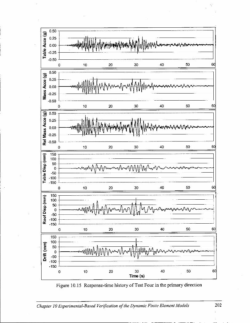
_ 0.50 ^ 0.25
0.00 a> S -0.25 ra
H -0.50
——t^m H 10 20 30 40 50 60
p- 150 E 100
50 0
-50 -100 -150
a w Q o n H
10 20 30 40 50 60
E E, a. to o o
150 100 50 0
-50 -100 -150
10 20 30 40 50 60
E E, £ Q
30 Time (s)
Figure 10.15 Response-time history of Test Four in the primary direction
Chapter 10 Experimental-Based Verification of the Dynamic Finite Element Models 202
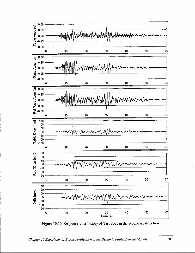
E E. a W a a> ra
150 100 50
0 -50
-100 -150
10 20 30 40 50 60
E E, a. M
O O
150 100 50 0
-50 -100 -150
\~
10 20 30 40 50 60
E E,
Q
Figure 10.16 Response-time history of Test Four in the secondary direction
Chapter 10 Experimental-Based Verification of the Dynamic Finite Element Models 203

10.2. Prediction of the dynamic behaviour of three-dimensional buildings
Because of the limitation of the LightFrame3D programs that the input excitation
history can consider one horizontal and one vertical earthquake components, the prediction
was only applicable to the building in Test Three exposed to a unidirectional ground motion.
The data from Test Four is reserved for future verifications once the program is further
expanded.
10.2.1. Natural frequencies and mode shapes
The predicted three fundamental frequencies using the LightFrame3D_Eigen program
are listed in Table 10.3, compared to the fundamental frequencies obtained from the sine
wave sweep test. Good agreements were achieved. The corresponding mode shapes drawn
from the eigenvectors given by the program are presented in Figure 10.17. These mode
shapes can also be compared to the results obtained from the sine wave sweep tests as
discussed in Section 10.1.1.
Table 10.3 Comparison of natural frequencies obtained from Test Three and predicted by
LightFrame3D program (Hz)
Data Source First Second Third
Test Three 2.9 5.1 8.8
LightFrame3D 2.8 6.1 8.8
Chapter 10 Experimental-Based Verification of the Dynamic Finite Element Models 204

M O D E 1 (fl = 2.8Hz)
M O D E 2 (£2 = 6.1Hz)
M O D E 3 (f3 = 8.8Hz)
Figure 10.17 Predicted three mode shapes
Chapter 10 Experimental-Based Verification of the Dynamic Finite Element Models 205
10.2.2. Comparison of predicted building behaviour and results from Test Three
Table 10.4 gives the peak values of drifts and accelerations during the first and
second large amplitude events from the dynamic tests and the analytical prediction. The
torsional motions and the occurrence times from experimental and analytical data are also
compared. Similar to the static predictions (see Section 9.2 in Chapter 9), the numerical
results from five points on the roof of building were used to calculate drift, relative mass
acceleration, and torsional motions. Among these points, three (one at the center of the roof
and two at the north and south corners) provided data of the drift and relative acceleration of
the building in the x direction, and two (at the east and west corners) provided data in the y
direction. The difference in the displacements measured at two opposite points (e.g. the
north and south corners) was calculated and then divided by the span of the roof to obtain the
angle of roof rotation. The rotational results in both x and y directions were similar, but not
identical due to slight changes in the roof geometric shape, because the roof was not perfectly
rigid. Figure 10.18 compares the drifts and relative mass accelerations of the building,
measured at the center position from the test and the simulation. It can be seen that the
numerically predicted response (drift and mass acceleration) follows the trends of the test
curves very well with similar cyclic frequency and vibration amplitude. The relative mass
accelerations predicted by the program and measured in the tests were processed by FFT to
obtain the acceleration response spectra and to compare the frequency components, as shown
in Figure 10.19. The measured and predicted frequencies corresponding to the maximum
response were 1.37 Hz and 1.39 Hz, respectively. They were very close to the frequency of
the input earthquake excitation (1.35 Hz, see Chapter 8). These results demonstrate that the
LightFrame3D program can predict the dynamic response of a building subjected to
Chapter 10 Experimental-Based Verification of the Dynamic Finite Element Models 206
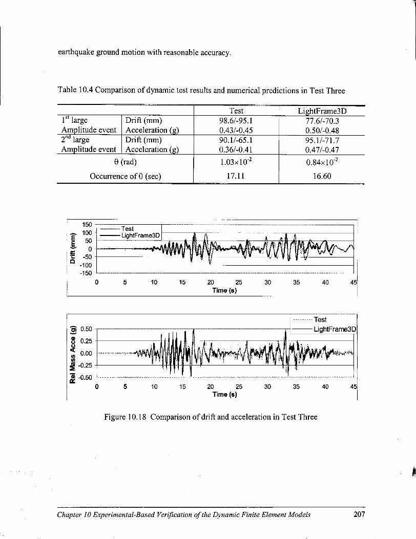
earthquake ground motion with reasonable accuracy.
Table 10.4 Comparison of dynamic test results and numerical predictions in Test Three
Test LightFrame3D 1 s t large Drift (mm) 98.6/-95.1 77.6/-70.3 Amplitude event Acceleration (g) 0.43/-0.45 0.50/-0.48 2 n d large Drift (mm) 90.1/-65.1 95.1/-71.7 Amplitude event Acceleration (g) 0.36/-0.41 0.47/-0.47
0 (rad) 1.03xl0"2 0.84xl0"2
Occurrence of 0 (sec) 17.11 16.60
Chapter 10 Experimental-Based Verification of the Dynamic Finite Element Models 207

0.020 Test LightFrame3D
0 .015 T3
g 0 .010 <
< 0.005
0.000 f
0 2 3 4 5 6 Frequency (Hz)
Figure 10.19 Comparison of acceleration frequency range
Figure 10.20 compares the top drift of all four walls in Test Three to help understand
the deformations in the buildings. Generally speaking, the graphs show that the numerically
predicted deformations in four walls match the test curves very well. When closely
examining the period between the 15th second and the 21st second of the first pulse (Figure
10.20 (a) and (b)), however, it is found that the predicted drifts in the north and south shear
walls were smaller than those obtained from the test. The difference in the north shear wall
with the opening was more significant than that in the south shear wall. The reasons are
believed to be the same as those discussed in the proceeding chapter. The predicted drifts in
the north and south shear walls also led a smaller maximum rotational angle, 6, when
compared to the value from the test, because both of them occurred within the above-
mentioned period. The reason for this discrepancy is likely that in this time period, the
severe strike of the first major component of the earthquake to the building has already
caused the failure of the test building, which was clearly observed in the test. This outcome
exceeded what had been planned for the model verification purpose. Usually, under such an
Chapter 10 Experimental-Based Verification of the Dynamic Finite Element Models 208

extreme condition, finite element programs may be difficult to reach a convergence. The
newly developed program overcame this difficulty successfully and ran through all
designated time steps, owing to the self-adaptive procedures implemented in the program.
However, the program may not accurately predict the actual building performance under this
situation. It is expected, by reviewing other time periods in the prediction, that the program
could provide better results i f the input ground acceleration were not so severe. From the
curves presenting the deformations of two transverse end walls, it can be seen that these two
walls vibrated with higher frequency than the two shear walls. This was an indication that
the movements of the two end walls were excited by the building's second and third natural
frequency and their modal responses therefore contributed mainly to the translation in the
short span and the rotational motion of the test building.
150 1 100 r 50 £ 0 2 -50 § -100 fc -150
— — T e s t 1 I I I » J M 1 LightFrame3D
_» l | | i t& Al l nMJUf t/ IA . A A A j \
* 1 V 1 f V
10 20 30 Time (s)
40 50 60
(a) North shear wall
E E,
Q o &
150 100 50 0
-50 -100 -150
Test LightFrame3D
**\A' /I A (IfIIM/WV \f<%
f V V V V ~ v
10 20 30 Time (s)
40 50 60
(b) South shear wall
Chapter 10 Experimental-Based Verification of the Dynamic Finite Element Models 209

-15 10 20 30
Time (s) 40 50 60
(c) East end wall
(d) West end wall
Figure 10.20 Comparisons of drifts of four walls in Test Three
10.3. Failure modes
Under the seismic loading, similar to the static loading, the observed predominant
failure in test buildings first occurred in the connections between the panels and framing
members. The local deformation zone of a nail connection under the significant seismic
(cyclic in nature) loading, however, showed a different pattern from that under a much
slower static monotonic loading. Under the earthquake excitation, the nail connectors bent
repeatedly in reversed directions and crushed the surrounding wood medium in different
locations. While the nail hole in the framing members was enlarged, a gap between the nail
shank and the wood fiber was formed and propagated, and nail withdrawal from wood
members occurred. This nail deformation impaired the energy dissipation ability of the
system due to the pinching of the hysteresis loops and caused degradation of the stiffness and
Chapter 10 Experimental-Based Verification of the Dynamic Finite Element Models 210

load carrying capacity of the system. At some locations, mostly along the edges of panels,
the nails pulled through the panels. A combination of both nail actions eventually led to the
systematic failure of the entire structure.
The observations from Test Three, under the unidirectional seismic loading, indicated
that the building experienced similar damage to the building in the static Test Two. The
failures were mostly presented in the two shear walls (north and south walls) in the forms of
nail withdrawal from framing and nail pulling through sheathing (Figure 10.21). Although
relative movements between the panels and frame members were observed in the two
transverse walls, permanent structural deformations were insignificant and nail failures did
not occur (Figure 10.22). Whether the failure first originated in the north shear wall with
opening or the south shear wall, however, was inconclusive from the test results owing to the
rapid excitation.
Figure 10.21 Nail withdrawal and pulling through failure modes
Chapter 10 Experimental-Based Verification of the Dynamic Finite Element Models 211
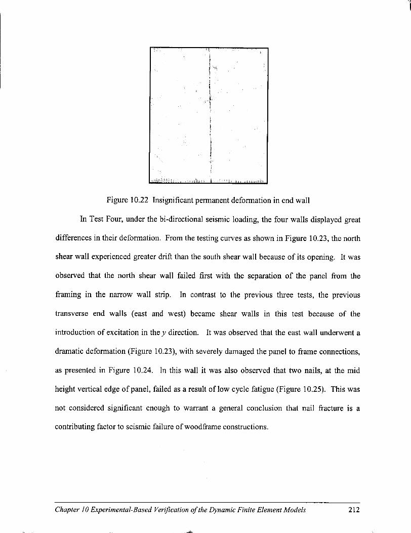
I ! ! : I
Figure 10.22 Insignificant permanent deformation in end wall
In Test Four, under the bi-directional seismic loading, the four walls displayed great
differences in their deformation. From the testing curves as shown in Figure 10.23, the north
shear wall experienced greater drift than the south shear wall because of its opening. It was
observed that the north shear wall failed first with the separation of the panel from the
framing in the narrow wall strip. In contrast to the previous three tests, the previous
transverse end walls (east and west) became shear walls in this test because of the
introduction of excitation in the y direction. It was observed that the east wall underwent a
dramatic deformation (Figure 10.23), with severely damaged the panel to frame connections,
as presented in Figure 10.24. In this wall it was also observed that two nails, at the mid
height vertical edge of panel, failed as a result of low cycle fatigue (Figure 10.25). This was
not considered significant enough to warrant a general conclusion that nail fracture is a
contributing factor to seismic failure of woodframe constructions.
Chapter 10 Experimental-Based Verification of the Dynamic Finite Element Models 212
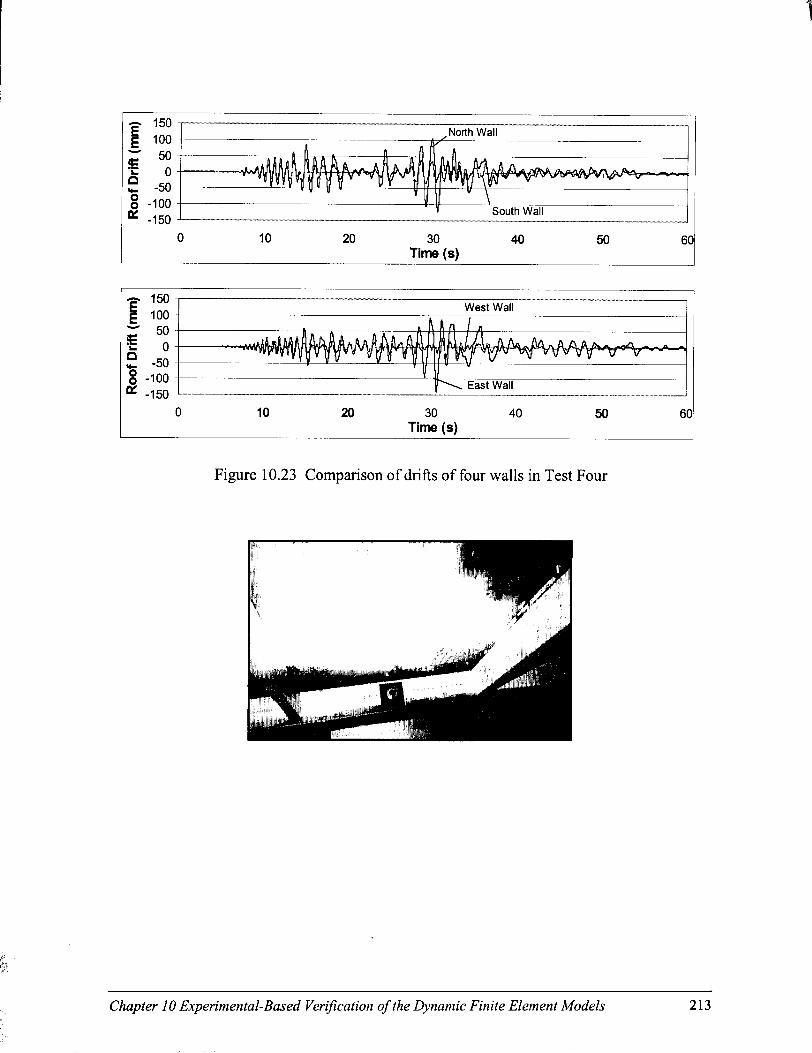
Figure 10.23 Comparison of drifts of four walls in Test Four
Chapter 10 Experimental-Based Verification of the Dynamic Finite Element Models 213
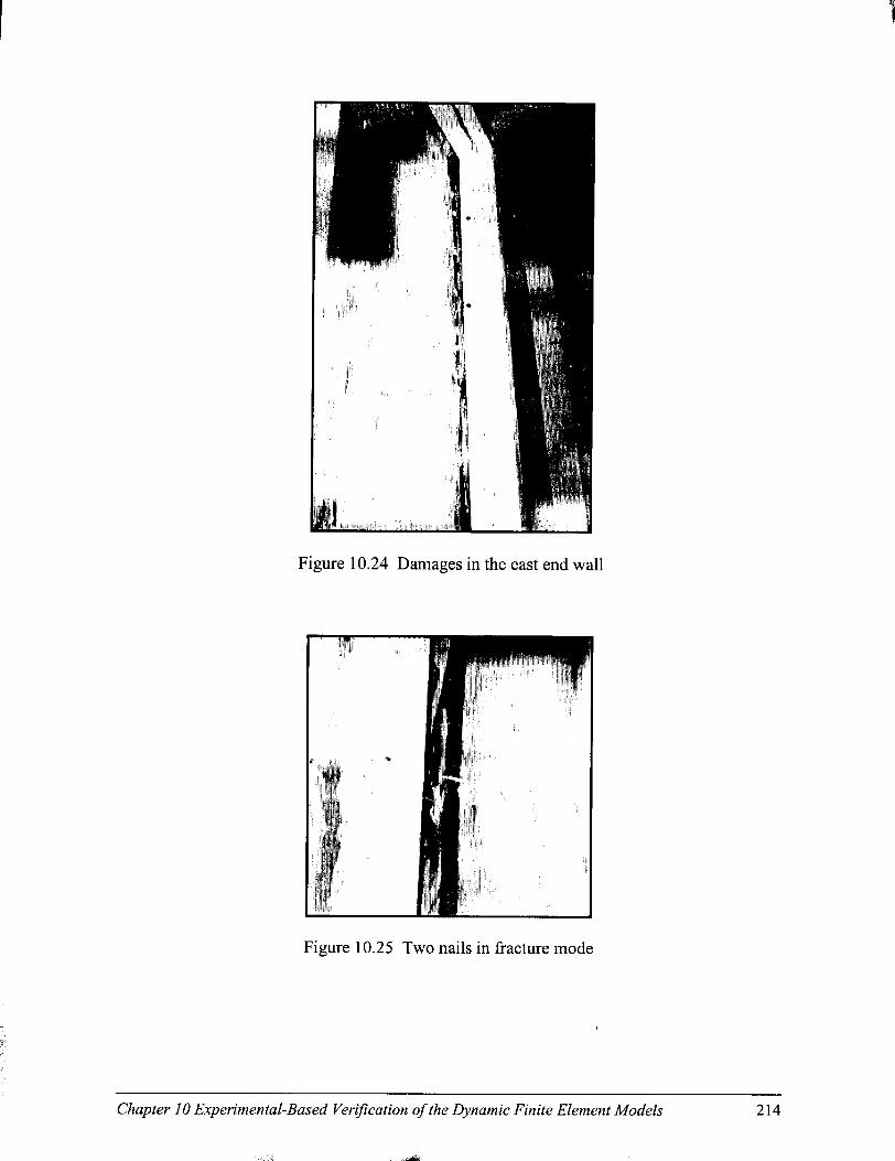
Figure 10.24 Damages in the east end wall
Figure 10.25 Two nails in fracture mode
Chapter 10 Experimental-Based Verification of the Dynamic Finite Element Models 214
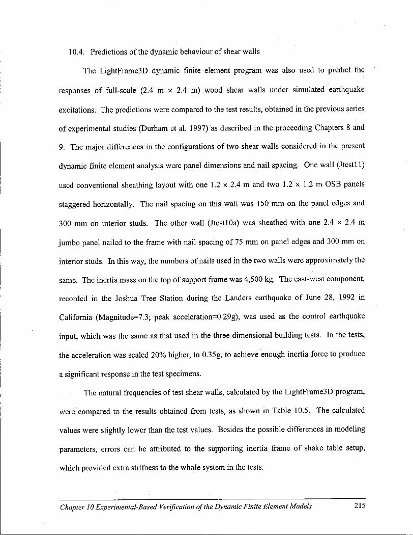
10.4. Predictions of the dynamic behaviour of shear walls
The LightFrame3D dynamic finite element program was also used to predict the
responses of full-scale (2.4 m x 2.4 m) wood shear walls under simulated earthquake
excitations. The predictions were compared to the test results, obtained in the previous series
of experimental studies (Durham et al. 1997) as described in the proceeding Chapters 8 and
9. The major differences in the configurations of two shear walls considered in the present
dynamic finite element analysis were panel dimensions and nail spacing. One wall (Jtestl 1)
used conventional sheathing layout with one 1.2 x 2.4 m and two 1.2 x 1.2 m OSB panels
staggered horizontally. The nail spacing on this wall was 150 mm on the panel edges and
300 mm on interior studs. The other wall (JtestlOa) was sheathed with one 2.4 x 2.4 m
jumbo panel nailed to the frame with nail spacing of 75 mm on panel edges and 300 mm on
interior studs. In this way, the numbers of nails used in the two walls were approximately the
same. The inertia mass on the top of support frame was 4,500 kg. The east-west component,
recorded in the Joshua Tree Station during the Landers earthquake of June 28, 1992 in
California (Magnitude=7.3; peak acceleration^.29g), was used as the control earthquake
input, which was the same as that used in the three-dimensional building tests. In the tests,
the acceleration was scaled 20% higher, to 0.35g, to achieve enough inertia force to produce
a significant response in the test specimens.
The natural frequencies of test shear walls, calculated by the LightFrame3D program,
were compared to the results obtained from tests, as shown in Table 10.5. The calculated
values were slightly lower than the test values. Besides the possible differences in modeling
parameters, errors can be attributed to the supporting inertia frame of shake table setup,
which provided extra stiffness to the whole system in the tests.
Chapter 10 Experimental-Based Verification of the Dynamic Finite Element Models 215
Table 10.5 Comparison of natural frequencies of shear walls predicted by LightFrame3D
program and measured from experiments
Shear Wall Natural frequency (Hz)
Test LightFrame3D
Jtest 11 - 1.2 x 2.4 Regular Panels 3.3 2.9
Jtest 10a - 2.4 x 2.4 Jumbo Panel 4.5 4.0
Table 10.6 gives the peak values of drifts and accelerations in the first and second
large amplitude shakes from the predictions and the tests. Figure 10.26 and Figure 10.27
display the predicted structural responses for both shear walls by the program, compared to
the test results. It is observed that the predicted drifts and relative mass accelerations follow
the test curves very well, with similar cyclic frequencies and vibration amplitudes.
Table 10.6 Comparison of maximum drifts and accelerations of shear walls predicted by
LighfFrame3D program and measured from experiments
Jtest 11 Jtest 10a
Test F E M Test F E M
1 s t large Disp. (mm) 37.3A32.6 26.4A52.4 8.4/-13.0 11.7/-20.0
Amplitude event Acce. (g) 0.42/-0.37 0.43/-0.36 0.47/-0.44 0.40/-0.40
2 n d large Disp. (mm) 51.7/-60.0 43.4/-61.9 14.1/-13.9 15.6/-22.4
Amplitude event Acce. (g) 0.28/-0.35 0.52/-0.37 0.52/-0.51 0.32/-0.39
Chapter 10 Experimental-Based Verification of the Dynamic Finite Element Models 216

15 20 25 Time (s)
30 35 40
Figure 10.26 Dynamic responses of shear wall with 4 by 8 regular panels
60 _ 40 I 20
¥ ° £ -20 ° -40
-60
——— JTestlOa
10 15 20 25 Time (s)
30 35 40
Figure 10.27 Dynamic responses of shear wall with one jumbo panel
The accelerograms on top of shear walls predicted by the program and measured in
the tests were then processed by FFT to obtain the Fourier spectra and to compare the
frequency components, as shown in Figure 10.28 (a) and (b). For shear wall Jtestll, the
maximum normalized amplitudes for both test and prediction have the same frequency of
Chapter 10 Experimental-Based Verification of the Dynamic Finite Element Models 217

1.34 Hz, whereas for shear wall JtestlOa, they are 1.44 Hz and 1.41 Hz, respectively. They
are all very close to the frequency of input earthquake excitation (1.35 Hz, see Chapter 8).
The FFT analysis indicated that the program could accurately predict the behaviour of test
specimens.
03 •o 3
0.020
0.015
E 0.010 < of u o < 0.005
0.000
Jtest11 • LightFrame3D
2 3 4 5
Frequency (Hz)
(a) Shear wall Jtestl 1 -1.2 x 2.4 m OSB sheathing panels
0.05
0.04 0) •o 3 = 0
Q. E < oi 0 o o <
03
.02
0.01
0.00
•JtestlOa • LightFrame3D
2 3 4 Frequency (Hz)
(b) Shear wall JtestlOa - single 2.4 x 2.4 m OSB sheathing panel
Figure 10.28 Comparison of Fourier spectra of shear walls predicted by LightFrame3D
program and from tests
Chapter 10 Experimental-Based Verification of the Dynamic Finite Element Models 218

10.5. Further expansion of the program
In numerical dynamic analysis, it is generally believed that the simulation of a
nonlinear wood light-frame system with a larger number of degrees of freedom is
computationally demanding (Folz et al. 2001). The dynamic finite element program
developed in this study also faces the same problem. The solution for this problem depends
on the developments in two areas. The first area is in computer technology and the second is
in numerical solution method. With the rapid development in computer technology, the
maximum C P U speed has been increased rapidly in recent years. Memory communication
bandwidths are much broader and storage capacities are increasing as well. For example, the
time spent on a dynamic analysis by using a P4 1.7 GHz computer could be 4.25 times
shorter than the time of running the same problem in a PHI 500 M H z computer. In solution
method area, the so-called "parallel processing" technique can be adopted to effectively
reduce computational time. The fundamental concept of parallel processing is that a program
is decomposed so that different data or instructions can be distributed among multiple
processors, allowing simultaneous execution of a program. This technique can be applied at
matrix level or within a do-loop, such as an element do-loop or Gauss point do-loop
(including nail connections). Several commonly used mechanisms in parallel processing are
standardized and are available in computer workstations and clusters. To perform parallel
processing, the program has to be modified to comply with parallel processing requirements.
It is evident that in an actual three-dimensional wood structure, only a few major
components are subject to significant and permanent deformations, while in others, the
deformation is insignificant and recoverable. This provides the possibility to save
computational time by approximating non-critical components, such as transverse walls,
Chapter 10 Experimental-Based Verification of the Dynamic Finite Element Models 219

floors and roofs, as i f they behave linearly. In addition, combining a few smaller elements
into a larger element by redistributing the nail connections to form an equivalent system can
also reduce the number of nodes and elements and, therefore, the computational time. This
method may be more appropriate for non-critical components than for major load carrying
components. The disadvantages of using these two methods in the simplified structural
model are that the solution may not have the required accuracy level and that local
deformation details may be overlooked.
It is believed that some other possible improvements are also important:
(1) In practice, an actual building might be subjected to multiple earthquakes and the
damage might be accumulative over time. To account for this phenomenon, there are
two options. If all the earthquake records are known before the simulation, these records
can be formed into a long record. In case the record that needs to be used in the
simulation is not handy, the program should be modified to be capable of saving data
from one case to another case to satisfy the requirement of multiple earthquake
simulations;
(2) To improve program prediction accuracy and to better reflect the actual behaviour of a
modeled wood-frame structural system, the failure models of frame member, panel, and
especially the nail connection should be investigated and implemented in the program
gradually; and
(3) In preprocessing stage, preparing an input data file for a large problem to be modeled in
the finite element analysis can be very tedious and prone to errors. To increase the data
input accuracy and efficiency, a sophisticated and user-friendly graphic interface in the
preprocessor is essential.
Chapter 10 Experimental-Based Verification of the Dynamic Finite Element Models 220

CHAPTER 1 1
CONCLUSIONS
This thesis describes in detail the development of three-dimensional nonlinear static
and dynamic finite element models for the study of wood light-frame structures, and
addresses the issues related to the behaviour of wood light-frame buildings subjected to
external loading. The experimental investigations of simplified three-dimensional buildings
were integrated into the thesis work. The accomplishments are as follows:
(1) Two three-dimensional nonlinear finite element models were developed. The programs
with the models implemented are capable of predicting the structural behaviour of
general wood light-frame buildings and their components under either static monotonic
and cyclic loading or seismic ground motion. A three-dimensional coordinate
transformation system is introduced into the programs to make the analysis of entire
building possible. "Substructuring" technique increases the effectiveness of the
coordinate transformation procedures and displays the force and deformation fields of
panel elements in a conventional way. The displacement history as one of the input
options is developed in the programs. This function allows the analysis to follow entire
deformation path to trace post-peak behaviour of a structure in a static monotonic
analysis and to study the energy dissipation and stiffness and strength degradation
characteristics of a structure in a static cyclic analysis. The programs were also equipped
Chapter 11 Conclusions 221
with several self-adaptive procedures to handle the difficulties in solution and iteration,
which ensure the programs to be robust and reliable;
(2) The uniqueness of the programs is the implementation of a mechanics based
representation of the load-deformation characteristics of individual panel-to-frame nail
connections in the diaphragm system. This approach believes that the hysteresis
behaviour is the structural response controlled by nonlinear characteristics of nail
connector and the surrounding wood medium. By using finite element approach, the
model simulates the nail connector as elasto-plastic beams acting on a nonlinear
foundation. Differently from other connection models, this model is not a test-dependent
curve-fitting model. It requires only the basic material properties of the connectors and
the embedding characteristics of the surrounding wood medium. This model represents
more accurately the actual hysteresis behaviour of connections and therefore the
programs with this model implemented can provide better predictions on the structural
behaviour of woodframe systems;
(3) One three-dimensional finite element program was developed to predict the fundamental
frequencies and mode shapes of wood structural system, and also provide the damping
coefficient required in the dynamic analysis;
(4) The algorithms of programs were carefully examined and tested step by step to ensure
the fundamental correctness. The models were thoroughly verified by means of
mechanics theories. This verification was carried out mainly in linear elastic range. A l l
of the results testing the beam deflections and stresses given by the models agreed to the
theoretical results with an error margin less than 5%, which tended to decrease with
increasing the number of elements;
Chapter 11 Conclusions 222

(5) Four tests on the full-scale simplified three-dimensional light-frame buildings were
conducted under both static and dynamic loading conditions. The tests provided an
excellent opportunity to observe and investigate the structural performance, system
effects, and failure modes in three-dimensional buildings. They also provided much
information for performing the experimental based model verification; and
(6) The models, combined with the experimental results, were applied to address the issues
in system effects, such as load sharing among the structural components, torsional
motion, and failure modes. The results suggest that the models can well display the
deformation patterns of the system under investigation, but the accuracy needs to be
further improved.
In the study of structural behaviour of three-dimensional wood light-frame buildings
using the newly developed finite element programs and experimental procedures, it was
observed that
(1) Compared to the static experimental results obtained from the three-dimensional building
tests and the previous two-dimensional shear wall tests, the maximum load carrying
capacities and the deflections at the ultimate load predicted by the static finite element
program showed differences less than 6% and 10%, respectively. The finite element
program calculated the test buildings with the same deformation pattern as shown in
tests; however, the predicted torsional rotations of test buildings were smaller than those
in tests. Under the cyclic loading, the finite element program well predicted the pinch
shaped hysteresis loops, energy dissipations, and strength and stiffness degradations in
shear wall systems. The program also successfully performed predictions of post-peak
cyclic behaviour of both three-dimensional building and two-dimensional shear wall;
Chapter 11 Conclusions 223

(2) Compared to the dynamic experimental results obtained from the three-dimensional
building test and the previous two-dimensional shear wall tests, the dynamic finite
element program provided satisfactory accuracy in the results of drifts, relative mass
accelerations, acceleration response spectra, and torsional motions (in 3D cases) of test
systems. The numerically predicted curves followed the test curves very well with
similar cyclical frequencies and amplitudes. It was also demonstrated that the finite
element program can calculate the eigenvalues for the natural frequencies and the
eigenvectors for the mode shapes of the test system, excellently matching the test results;
(3) In the preliminary study of system effects, the results obtained from the finite element
programs suggested that the shear wall with higher stiffness carried most of the lateral
load applied to the building, and the transverse walls perpendicular to the load direction
shared notable lateral forces even though no external load was applied to them directly.
It was also found that the load sharing mechanism can redistribute the stiffness of
components, and therefore the total deformation and load carrying capacity of a system
are not simple addition of those possessed by the individual components in the system;
and
(4) The finite element programs effectively predicted the movements of sheathing and
framing of a test building. The path of nail failure and the maximum forces in nail
connectors were also reasonably calculated. Due to the limitations of the program,
however, the detailed nail failure modes in nail withdrawal from the framing and nail
pulling through the sheathing panel cannot be displayed.
In addition, the following can be concluded for the experimental study:
(1) Under statically applied mono tonic load, the buildings with or without dead load showed
Chapter 11 Conclusions 224
similar load carrying capacity. The ability to sustain load capacity after the ultimate load
level in the building with dead load was less than that in a building without dead load,
which may be explained by the P-A effect caused by the dead load on the top of building;
and
(2) In Test Four where the test building was subject to bi-directional seismic excitations, the
building experienced substantially greater torsional motion with larger drifts in both
directions than the building subjected to only unidirectional seismic loading. This
implies that when a building is subjected to bi- or multi-direction ground motions, the
effect could be cumulative and the damage could be much more severe.
The thesis also discusses the necessary and possible improvements to be implemented
into the newly developed finite element programs. The improvements are mainly focused on
how to promote the efficiency of the programs by saving significant computational time and
how to enhance the ability of the programs to predict the detailed localized deformations with
higher accuracy.
The preliminary application of the static and dynamic nonlinear finite element
programs shows that they can predict the behaviour of wood light-frame structures with good
accuracy and, more importantly, they can suit a wide range of structural, material and loading
variations. The programs are expected to be useful either in analysis of an individual
structure or in construction of response surfaces for reliability assessment of general wood
structures. Such analyses can be used to develop design rules for wood frame systems. It is
also believed that the programs will be useful tools in performing the parametric study of
three-dimensional buildings to provide better understanding of system effects which
influence the overall structural behaviour of wood light-frame systems.
Chapter 11 Conclusions 225
BIBLIOGRAPHY
American Society for Testing and Materials (ASTM) (1996). "Proposed standard method of
cyclic (reversed) load test for shear resistance of framed walls for buildings." Philadelphia,
USA.
American Society for Testing and Materials (ASTM) (1993). "Proposed standard test method
for dynamic properties of connections assembled with mechanical fasteners (3rd Draft)."
Philadelphia, USA.
Andreasson, S. (1999). "Three-dimensional interaction in stabilization of multi-storey timber
frame buildings." Proc. of International Council for Building Research Studies and
Documentation, Working Commission W18 - Timber Structures, Meeting Thirty-Two,
Graz, Austria.
Baber, T. and Wen, Y . K . (1981). "Random vibration of hysteretic degrading systems." J. of
Engrg. Mechanics, A S C E , 107(6), 1069-1089.
Baber, T. and Noori, M . N . (1985). "Random vibration of degrading, pinching systems." J. of
Engrg. Mechanics, A S C E , 111(8), 1010-1026.
Bathe, K-J . (1996). Finite Element Procedures. Prentice-Hall, Inc., New Jersey, NJ.
Bendat, J.S. and Piersol, A . G . (1986). Random data: analysis and measurement procedures.
John Wiley & Sons, Inc. New York, N Y .
Bibliography 226
Boughton, G.N. (1982). "Simulated wind tests on a house: part 1 - description and part 2 -
results." Technical Reports No. 12 and No. 14, Cyclone Testing Station, James Cook
University of North Queensland, Townsville, Australia.
Boughton, G.N. and Reardon, G.F. (1984). "Simulated wind tests on the Tongan hurricane
house." Tech. Rep. No. 23, James Cook Cyclone Structural Testing Station, Townsville,
Queensland, Australia.
Boughton, G.N. (1988). "Full-scale structural testing of houses under cyclonic wind loads."
Proc. 1988 Int. Timber Engrg. Conf, Ed.: Itani, R.Y. , Forest Products Research Society,
Madison, WI, 2:82-87.
Case, P.C., and Isyumov, N . (1995). "Initial study of the performance of a wood structure
with a pitched roof slope of 4:12 under extreme wind loads." Draft Report, BLWTL-SS-
1995, for Canadian Wood Council and American Forest and Paper Association, Faculty of
Engrg. Sci., Univ. of Western Ontario, ON.
Ceccotti, A . , Follesa, M . and Karacabeyli, E. (2000). "3D seismic analysis of multi-storey
wood frame construction." Proc. World Conference on Timber Engineering, Whistler, B.C.
Chehab, M . (1982). "Seismic analysis of a two-story wood framed house using the response
spectrum technique." M.Sc. Dissertation, Dept. of Civi l Engrg, Oregon State Univ.,
Corvallis, OR.
Chopra, A . K . (1995). Dynamics of structures. Prentice-Hill, Inc., New Jersey, NJ.
Comite' Europeen de Normalisation (CEN) (1995). "Timber structures - Test methods -
Cyclic testing of joints made with mechanical fasteners (Draft)." E N TC 124.117,
European Committee for Standardization, Brussels, Belgium.
Cook, R.D., Malkus, D.S., and Plesha, M.E . (1989). Concepts and applications of finite
Bibliography 227
element analysis. 3rd Ed., John Wiley & Sons, New York, N Y .
Dolan, J.D. (1989). "The dynamic response of timber shear walls." Ph.D. Dissertation, Dept.
of Civi l Engineering, Univ. of British Columbia, Vancouver, B.C.
Durham, J., Prion, H.G.L., Lam, F., and He, M . (1997). "Earthquake resistance of shear walls
with oversized sheathing panels." Proc. Recent Advances in Understanding Full-Scale
Behavior in Wood Buildings, Forest Prod. Soc, Madison, WI, 57-64.
Durham, J. (1998). "Seismic response of wood shearwalls with oversized oriented strand
board panels." M.A.Sc. Dissertation, Dept. of Civi l Engineering, Univ. of British
Columbia, Vancouver, B.C.
Durham, J., He, M . , Lam, F., and Prion, H . G.L. (1998). "Seismic resistance of wood shear
walls with oversize sheathing panels." Proc. of 5th World Conf. on Timber Engrg.,
Lausanne, Switzerland, 1:396-403.
Durham, J., Prion, H. G.L., Lam, F., and He, M . (1999). "Earthquake resistance of shearwalls
with oversize sheathing panels." Proc. of 8th Canadian Conf. on Earthquake Engineering,
Vancouver, B.C.
Filiatrault, A. , Uang, C - M . and Seible, F. (2000). "Ongoing seismic testing and analysis
program in the CUREe-Caltech woodframe project in California." Proc. World Conference
on Timber Engineering, Whistler, B.C.
Foliente, G.C. (1993). "Stochastic dynamic response of wood structural systems." Ph.D.
Dissertation, Virginia Polytechnic Ins. and State Univ., Blacksburg, V A .
Foliente, G.C. and Zacher, E.G. (1994). "Performance tests of timber structural systems
under seismic loads." Proc. of a Research Needs Workshop, University of California, CA.
Foliente, G.C. (1995). "Hysteresis modeling of wood joints and structural systems." J. of
Bibliography 228

Struct. Engrg., ASCE, 121(6), 1013-1022.
Foliente, G.C. (1997). "Timber structures in seismic regions: general overview and research
needs." Proc. of E.Q. Performance and Safety of Timber Struc, Forest Prod. Soc,
Madison, WI, 3-23.
Foliente, G . C , Paevere, P., Macindoe, L. , Banks, R. and Kasai, B . (2000). "System effects
and load-sharing in an L-shaped woodframe house." Proc. World Conference on Timber
Engineering, Whistler, B.C.
Folz, B., Filiatrault, A. , Uang, C - M . and Seible, F. (2001). "Blind prediction of the seismic
response of a two-story woodframe house: an international benchmark." Report No. SSRP-
2001/15, Univ. of California, San Diego, La Jolla, CA.
Foschi, R.O. (1974). "Load-slip characteristics of nails." Wood Sci., 7(1), 69-76.
Foschi, R.O. (1977). "Analysis of wood diaphragms and trusses, Part one: Diaphragms."
Can. J. Civ. Eng., 4(3), 345-352.
Foschi, R.O. (1997). "SSP: A general structural analysis for stressed-skin panels." Program
User's Manual prepared for SRI Homes International, Kelowna, B.C. , Dept. of Civil
Engineering, Univ. of British Columbia, Vancouver, B.C.
Foschi, R.O. (2000). "Modeling the hysteretic response of mechanical connections for wood
structrues." Proc. World Conference on Timber Engineering, Whistler, B.C.
Foschi, R.O. and Yao, F. (2000). "Determining embedment response parameters from
connector tests." Proc. World Conference on Timber Engineering, Whistler, B.C.
Gupta, A . K . and Kuo, G.P. (1985). "Behavior of wood-framed shear walls." J. of Struct.
Engrg., A S C E , 111(8), 1722-1733.
Gupta, A . K . and Kuo, G.P. (1987). "Modeling of a wood-frame house." J. of Struct. Engrg.,
Bibliography 229
A S C E , 113(2), 260-278.
Hall, J.F. (2000). "The CUREe-Caltech woodframe project." Proc. World Conference on
Timber Engineering, Whistler, B.C.
He, M . (1997). " A study of wood based shear walls sheathed with oversize oriented strand
board panels." M.A.Sc. Dissertation, Univ. of British Columbia, Vancouver, B.C.
He, M . , Lam, F., and Prion, H.G.L. (1998). "Influence of cyclic test protocols on
performance of wood based shear walls." Can. J. of Civil Engrg., NRC, 25,539-550.
Hirashima, Y . et al. (1981). "Studies on wood-panel construction (II) - loading test of full-
scale house." Bulletin of the Forestry and Forest Products Research Institute, No. 315,
Ibaraki, Japan.
Humar, J.L. and Kumar, P. (1998). "Torsional motion of buildings during earthquakes. II.
Inelastic response." Can. J. Civ. Eng., NRC, 25: 917-934.
Jackson, J.A. (1989). "Gravity load effects on lateral load resistance." M.S. Dissertation,
Washington State University, Pullman, WA.
Karacabeyli, E. (1995). "Lateral resistance of nailed shear walls subjected to static and cyclic
displacements." Proc. FPS 1995 Annual Meeting, Section on Seismic Safety of Timber
Structures, Portland, OR.
Karacabeyli, E. (1996). "Joints made with mechanical fasteners." Meeting notes of ISO TC
165 (Timber Structures) Working Group 7 Meeting, New Orleans, L A .
Kasai, B. , Leichti, R.J., and Itani, R Y . (1994). "Nonlinear finite-element model of complete
light-frame wood structures." J. of Struct. Engrg., ASCE, 120(1), 100-119.
Kasai, B., and Xu, H. (1997). " A mathematical model of connections with nonlinear
nonconservative hysteretic behavior." Proc. of E.Q. Performance and Safety of Timber
Bibliography 230

Struc, Ed.: Foliente, G . C , Forest Prod. Soc., Madison, WI.
Kasai, B., Collins, M . , Foliente, G . C , and Paevere, P. (1999). " A hybrid deterministic and
stochastic approach to inelastic modeling and analysis of light-frame buildings." Proc. 1st
Int. R I L E M Symposium on Timber Eng., Ed: Bostrom, L. , R I L E M publications,
Stockholm, Sweden, 61-77.
Kivell , T., Moss, P J . and Carr, A.J . (1981). "Hysteretic modeling of moment-resisting nailed
timber joints." Bull. New Zealand Nat. Soc. For Earthquake Engrg., Waikanae, New
Zealand, 14(4), 233-243.
Kohara, K . and Miyazawa, K. (1998). "Full-scale shaking table test of two story wooden
dwelling houses." Proc. of the Int. Conf. On Timber Engrg., Montreux, Switzerland, Vol .
2, 548-555.
Krawinkler, H. , Parisi, F., Ibarra, L. , Ayoub, A . and Medina, R. (2001). "Development of a
testing protocol for wood frame structures." Report of Task 1.3.2 of the CUREE-Caltech
Woodframe Project, Dept. of Civil and Env. Engrg., Stanford Univ., C A .
Lam, F., Prion, H.G.L., He, M . and Durham, J. (1998). "Earthquake resistance of wood based
shear walls with oversize sheathing panels." Proc. of Structural Engineering World Wide
1998, Ed: Srivastava, N.K. , Paper T222-4.
Latendresse, V . and Ventura, C E . (1995). "Shake table testing of 'Anti-Rakker' device for
playwood shear walls." Earthquake Engrg., Univ. of British Columbia, Vancouver, B.C.
McCutcheon, W.J. (1985). "Racking deformation in wood shear walls." J. of Struct. Engrg.,
ASCE, 111(2), 257-269.
Newland, D.E. (1986). An introduction to random vibrations and spectral analysis. 2 n d Ed.,
Longman Sci. & Tech., U K .
Bibliography 231

Ohashi, Y . , Sakamoto, I. and Kimura, M . (1998). "Shaking table tests of a real scale wooden
house subjected to Kobe earthquake." Proc. of the Int. Conf. On Timber Engrg., Montreux,
Switzerland, Vol . 2, 556-563.
Phillips, T.L., Itani, R.Y. , and McLean, D.I. (1993). "Lateral load sharing by diaphragms in
wood-framed buildings." J. of Struct. Engrg., A S C E , 119(5), 1556-1571.
Polensek, A . (1983). "Structural analysis of light-frame wood buildings." Proc. of the
Workshop on Structural Wood Research, State-of-the-art' and research needs, Eds, Itani,
R Y . and Faherty, K.F. , ASCE, 189-203.
Popov, E.P. (1952). Mechanics of materials. Prentice-Hall, Inc., New Jersey, NJ.
Pryor, S.E., Taylor, G.W. and Ventura, C E . (2000). "Seismic testing and analysis program
on high aspect ratio wood shear walls." Proc. World Conference on Timber Engineering,
Whistler, B.C.
Rainer, J.H. and Karacabeyli, E. (1998). "Wood-frame building construction in earthquakes."
Special Publication No. SP-40, Forintek Canada Corp., Vancouver, B.C.
Rainer, J.H. and Karacabeyli, E. (2000). "Wood-frame construction in past earthquakes."
Proc. World Conference on Timber Engineering, Whistler, B.C.
Schmidt, R.J. and Moody, R.C. (1989). "Modeling laterally loaded light-frame buildings." J.
of Struct. Engrg., ASCE, 115(1), 201-217.
Stewart, A . H . , Goodman J.R., Kliewer A . and Salsbury E . M . (1988). "Full-scale tests of
manufactured houses under simulated wind loads." Proc. of Int. Timber Engrg. Conf., 2:97-
111, Seattle, WA.
Stewart, W.G., Dean, J.A., and Carr, A.J . (1988). "The earthquake behavior of plywood
sheathed shearwalls." Proc. of Int. Timber Engrg. Conf., Ed.: Itani, R.Y. , Forest Products
Bibliography 232
Research Society, Madison, WI, 2:248-261.
Sugiyama, H. , Andoh, N . , Uchisako, T., Hirano, S., and Nakamura, N . (1988). "Full-scale
test of a Japanese type two-story wooden frame house subjected to lateral load." Proc. of
Int. Timber Engrg. Conf., Ed.: Itani, R.Y. , Forest Products Research Society, Madison, WI,
2:55-61.
Tanaka, Y . , Ohasi, Y . and Sakamoto, I. (1998). "Shaking table test of full-scale wood-framed
house." Proc. of the 10 t h Earthquake Engrg Symposium, Yokohama, Japan, 2487-2492. (In
Japanese)
Tarabia, A . M . and Itani, R .Y. (1997). "Seismic response of light-frame wood buildings." J.
of Struct. Engrg., ASCE, 123(11), 1470-1477.
Tuomi, R.L. and McCutcheon, W.J. (1974). "Testing of a full-scale house under simulated
snowloads and windloads." Res. Paper, FPL 234, U.S. Dept. of Agriculture, Forest Pro.
Lab., Madison, WI.
Timoshenko, S.P., and Woinowsky-Krieger, S. (1959). Theory of plates and shells. 2 n d Ed.,
McGraw-Hill Book, Inc., New York, N Y .
Timoshenko, S.P., and Goodier, J.N. (1970). Theory of elasticity. 3 r d Ed., McGraw-Hill
Book, Inc., New York, N Y .
Yamaguchi, N . and Minowa, C. (1998). "Dynamic performance of wooden bearing walls by
shaking table test." Proc. of the Int. Conf. On Timber Engrg., Montreux, Switzerland, Vol .
2, 26-33.
Yasumura, M . , Murota, T., Nishiyama, I, and Yamaguchi, N . (1988). "Experiments on a
three-storied wooden frame building subjected to horizontal load." Proc. of Int. Timber
Engrg. Conf., Ed. Itani, R.Y. , Forest Products Research Society, Madison, WI, 2:262-275.
Bibliography 233

APPENDIX A
PROGRAM USER'S MANUAL
A.1. Introduction
This user's manual provides the relevant background information for the
LightFrame3D nonlinear finite element programs. The programs are designed to analyze
three-dimensional wood light-frame constructions and their components or subassemblies,
under both static monotonic and cyclic loading (LightFrame3D_Static) and earthquake
excitation (LightFrame3D_Dynamic). Eigenvalues and corresponding eigenvectors can be
calculated by using LightFrame3D_Eigensolver, from which the natural frequencies and
mode shapes of the system can be derived. These programs address the common light-frame
building configurations and loading conditions in a versatile manner.
A.2. Modeling
A basic structural model in the program contains an exterior panel, frames, an
optional interior panel, and nail connections. The panels are connected to four frame
members by nails in a sandwich pattern. The case to be analyzed is meshed into a number of
four-side rectangular element units, which has four nodes with six nodal degrees of freedom
and one element degree of freedom. The nodal degrees of freedom represent three
translations in x, y and z directions (u, v, w), and three rotations about x, y and z axes (Rot-x,
Rot-y, Rot-z). The element degree of freedom is one twist in x-y plane (wxy). Connection
Appendix A Program User's Manual 234

elements have three degrees of freedom at each node (u, v, w). Four-point Gauss quadrature
is used in the programs. The nodes on an element should be numbered in a counterclockwise
direction. The pattern of numbering the entire mesh of a structure, however, should be
carefully decided, because it decides the bandwidth of the stiffness matrix in the problem to
be studied. Bandwidth will tremendously affect the size of the problem and hence the
computational time. A smaller bandwidth is desired.
The optional interior panels may have different material properties from those of the
exterior panels. When an interior panel is present, the space between the exterior and interior
panels may be filled with insulation material (EPS). The insulation is assumed to provide
support.to the sheathing panels when the buckling of the panels produces compression in the
insulation. Within an element, the four frame members may have different material
properties and dimensions. It can also be assumed that there is no frame member on certain
side(s) of the element. On each side of an element, the nail connection can be in different
types, material properties, dimensions and spacings. The analysis also applies to the models
with openings (e.g. doors or windows).
The programs can handle different loading combinations. In the static analysis, in-
plane concentrated loads and out-of-plane distributed loads can be applied simultaneously.
These loads may be constant or incremented individually in fixed or uneven steps. Load
control mode or displacement control mode is used as input history in static monotonic
analysis, whereas only displacement control mode is used in static cyclic analysis. In
dynamic analysis, earthquake excitations can be in horizontal and/or vertical directions. At
the same time, static constant loads can be applied to the structure.
The dynamic modal analysis procedure can be performed on the structure to obtain
Appendix A Program User's Manual 235
the natural frequencies and the corresponding mode shapes before the dynamic time-history
analysis is laid out. The fundamental frequency is needed to decide the damping coefficient
required by the program and is also an indicator in model verification. The inertia mass can
be consistent or lumped at nodes. The mass of panel and frame members may or may not be
considered. When it is considered, the mass of the panel and frame members can also be
consistent or lumped. The mass-proportional Reyleigh damping is used in the program.
The programs are written in Fortran 90. There is no limitation on the problem size
from the programs themselves, because of the use of dynamically allocated arrays. The
actual problem size that can be calculated and the computational time, however, heavily
depend on the computer system used. The minimum system requirement for personal
computers solving small to medium size problems is Pentium III 500 M H z and compatible
processor, 128 M B R A M , and 10GB hard disk drive. For large size problems, a workstation
or computer cluster is recommended.
Any unit system can be used in the programs. The unit should be consistent within
the problem. For example, i f forces are measured in Newton and coordinates in meter, the
stresses must be in N/m 2 , distributed loads in N/m 2 , and acceleration in m/s2.
For more detailed theoretical information, please refer to the context of this thesis.
A. 3. Input and output files
Four input data files may be needed in an analysis:
(1) Input file one: Titles. This file is a batch file containing the names and locations of input
data file, output file, and cyclic protocol file for static cyclic loading or earthquake record
for dynamic loading,
(2) Input file two: Input data. This is a text file containing all the information of the studied
Appendix A Program User's Manual 236

model. This file includes the three-dimensional nodal coordinates, material properties,
loading patterns, and boundary conditions,
(3) Input file three: Cyclic protocol. This file contains the displacement points for scheduled
loading cycles required in the static cyclic analysis, and
(4) Input file four: Time-acceleration history. This file can be a past earthquake record or a
simulated time-acceleration series required in the dynamic analysis.
The preprocessor generates the following files:
(1) A text file containing all the information given by the input data file (Input file two) and
relevant resultant parameters (*.tst),
(2) Files written in Lisp language to graphically present the meshes of panel and frame
elements (Meshtopcover.lsp, Meshframe.lsp, and Meshbtmcover.lsp),
(3) A file containing a new set of time-acceleration history actually used in the calculation
after defining the maximum acceleration increment (Accelerogram), which may not be
the same as the original one, and
(4) A file containing the first 10 lowest eigenvalues and corresponding eigenvectors of a
structure calculated by LightFrame3D_Eigensolver (Eigenvalues) for dynamic analysis.
The postprocessor generates the desired information in the following files:
(1) A text file containing general information of nodal displacements and forces (*.out),
(2) Files containing load-displacement points at specified locations (nodes) (PL*, up to five),
(3) Files containing panel stresses (Panelstress), frame stresses (Framestress), relative
displacements of panel and frame elements (Reladisp), and nail forces (Nailforce),
(4) File generated in Lisp language to graphically present the deformed shapes of the
structure (Defoshape.lsp), and
Appendix A Program User's Manual 237

(5) A script file generating slides which can be displayed in A u t o C A D 1 M and MS
Powerpoint™ software (Slides.scr).
The structures and applications of these files are described in the subsequent sections.
A.4. Structures and control parameters of input files
A.4.1. Input file one - Titles
Line 1. A title describing the problem, which will appear in the output file (*.out) and is up to
80 characters.
Line 2. Index for executive type.
0 - preprocessing.
1 - solving and post-processing.
Line 3. Input data file name.
For example:
D:\anybody\anysubdirectory\anycase.dat
Line 4. Output file name for 0 and 1 in Line 2.
For example:
D:\anybody\anysubdirectory\preproce.tst or
D:\anybody\anysubdirectory\solution.out
Line 5. Index for loading input.
0 - static monotonic loading and no further line in this file is needed.
1 - static cyclic loading.
2 - dynamic loading.
Line 6. If 1 or 2 is chosen in Line 5, give name of the file containing cyclic protocol or
dynamic time-acceleration history.
Appendix A Program User's Manual 238

For example:
D :\anybody\anysubdirectory\Joshua. acc
End of the input file one.
This file should be saved in the same directory where the executable file of the program is
located.
A.4.2. Input file two - Input data
Note: The appearance of characters ST (for static) and D Y (for dynamic) in a line or
following a control parameter indicates that the line or the parameter has to be included in the
corresponding data file for static analysis or dynamic analysis. If not specified, a line should
be in both static and dynamic data files.
Line 1. Number of plotting files, acceleration of gravity (DY). A maximum of five plotting
files can be opened and are automatically named as PL1, PL2, and so on. These files show
the calculated displacement and load results at specified locations (nodes).
MAXPL, GA
Line 2. Overall numbers of elements and nodes. Enter five numbers. They are:
1. Total number of exterior panel elements.
2. Total number of nodes in exterior panel elements.
3. Index for interior panel elements. 0 - No interior panel element; 1 - At least one
interior panel element.
4. If 1 is chosen in number 3, total number of nodes in interior panel elements;
otherwise 0.
5. Total number of frame nodes.
NELEM, NNODET, NELEMB, NNODEB, NNODEF
Line 3. Enter the number of Gaussian integration points along the connector span (x
Appendix A Program User's Manual 239
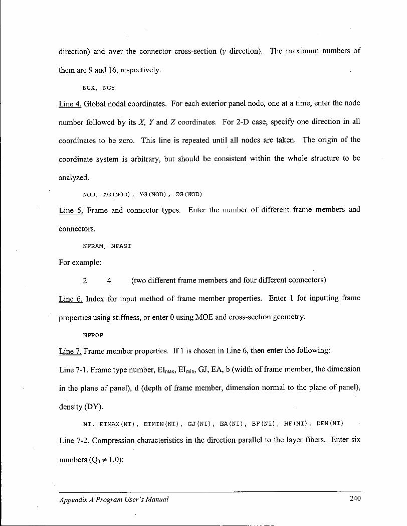
direction) and over the connector cross-section (y direction). The maximum numbers of
them are 9 and 16, respectively.
NGX, NGY
Line 4. Global nodal coordinates. For each exterior panel node, one at a time, enter the node
number followed by its X, Y and Z coordinates. For 2-D case, specify one direction in all
coordinates to be zero. This line is repeated until all nodes are taken. The origin of the
coordinate system is arbitrary, but should be consistent within the whole structure to be
analyzed.
NOD, XG(NOD), YG(NOD), ZG(NOD)
Line 5. Frame and connector types. Enter the number of different frame members and
connectors.
NFRAM, NFAST
For example:
2 4 (two different frame members and four different connectors)
Line 6. Index for input method of frame member properties. Enter 1 for inputting frame
properties using stiffness, or enter 0 using M O E and cross-section geometry.
NPROP
Line 7. Frame member properties. If 1 is chosen in Line 6, then enter the following:
Line 7-1. Frame type number, E I m a x , EI m j n , GJ, EA, b (width of frame member, the dimension
in the plane of panel), d (depth of frame member, dimension normal to the plane of panel),
density (DY).
NI, EIMAX(NI), EIMIN(NI), GJ(NI), EA(NI), BF(NI), HF(NI), DEN(NI)
Line 7-2. Compression characteristics in the direction parallel to the layer fibers. Enter six
numbers ( Q 3 * 1.0):
Appendix A Program User's Manual 240
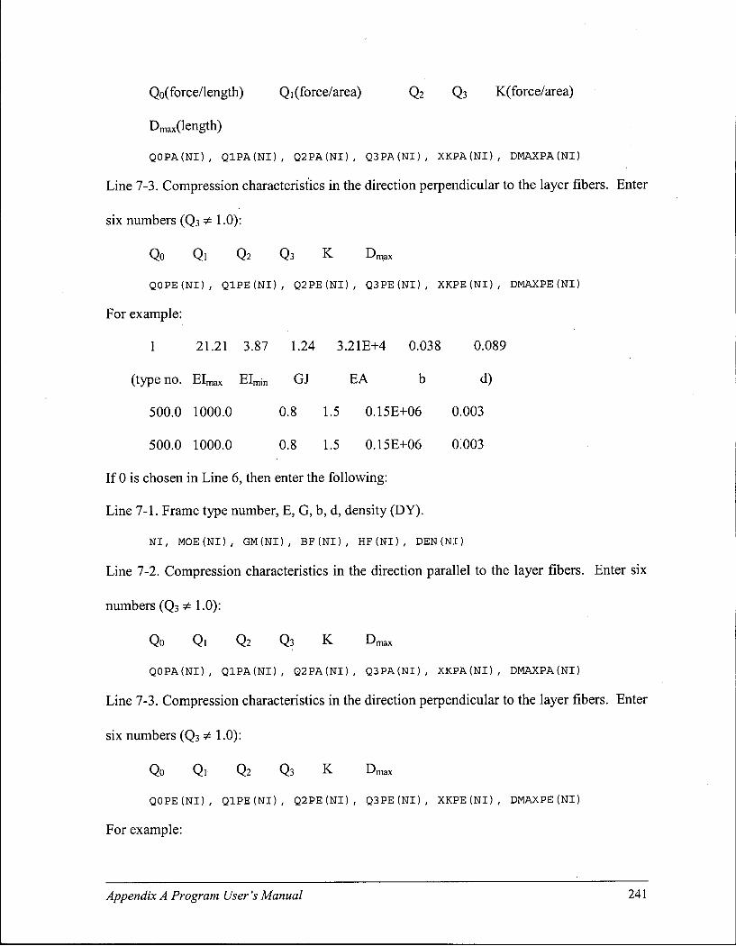
Qo(force/length) Qi (force/area) Q 2 Q3 K(force/area)
Dm a x(length)
QOPA(NI), QIPA(NI), Q2PA(NI), Q3PA(NI), XKPA(NI), DMAXPA(NI)
Line 7-3. Compression characteristics in the direction perpendicular to the layer fibers. Enter
six numbers (Q3 * 1.0):
Qo Qi Q2 Q3 K D m a x
QOPE(NI), QIPE(NI), Q2PE(NI), Q3PE(NI), XKPE(NI), DMAXPE(NI)
For example:
1 21.21 3.87 1.24 3.21E+4 0.038 0.089
(type no. E I m a x E I m i n GJ E A b d)
500.0 1000.0 0.8 1.5 0.15E+06 0.003
500.0 1000.0 0.8 1.5 0.15E+06 0.003
If 0 is chosen in Line 6, then enter the following:
Line 7-1. Frame type number, E, G, b, d, density (DY).
NI, MOE(NI), GM(NI), BF(NI), HF(NI), DEN(NI)
Line 7-2. Compression characteristics in the direction parallel to the layer fibers. Enter six
numbers (Q3 * 1.0):
Qo Qi Q2 Q3 K D m a x
QOPA(NI), QIPA(NI), Q2PA(NI), Q3PA(NI), XKPA(NI), DMAXPA(NI)
Line 7-3. Compression characteristics in the direction perpendicular to the layer fibers. Enter
six numbers (Q3 * 1.0):
Qo Qi Q2 Q3 K D m a x
QOPE(NI), QIPE(NI), Q2PE(NI), Q3PE(NI), XKPE(NI), DMAXPE(NI)
For example:
Appendix A Program User's Manual 241
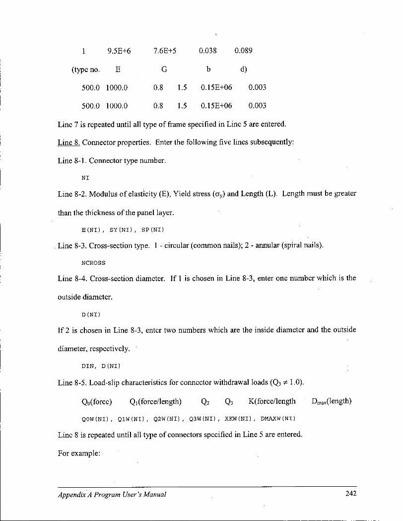
1 9.5E+6 7.6E+5 0.038 0.089
(type no. E G b d)
500.0 1000.0 0.8 1.5 0.15E+06 0.003
500.0 1000.0 0.8 1.5 0.15E+06 0.003
Line 7 is repeated until all type of frame specified in Line 5 are entered.
Line 8. Connector properties. Enter the following five lines subsequently:
Line 8-1. Connector type number.
NI
Line 8-2. Modulus of elasticity (E), Yield stress (ay) and Length (L). Length must be greater
than the thickness of the panel layer.
E(NI) , SY(NI), SP(NI)
Line 8-3. Cross-section type. 1 - circular (common nails); 2 - annular (spiral nails).
NCROSS
Line 8-4. Cross-section diameter. If 1 is chosen in Line 8-3, enter one number which is the
outside diameter.
D(NI)
If 2 is chosen in Line 8-3, enter two numbers which are the inside diameter and the outside
diameter, respectively.
DIN, D(NI)
Line 8-5. Load-slip characteristics for connector withdrawal loads (Q3 ^ 1.0).
Qo(force) Qi (force/length) Q 2 Qj K(force/length Dm a x(length)
QOW(NI), QIW(NI), Q2W(NI), Q3W(NI), XKW(NI), DMAXW(NI)
Line 8 is repeated until all type of connectors specified in Line 5 are entered.
For example:
Appendix A Program User's Manual 242
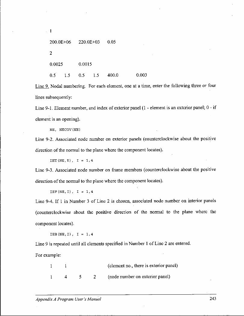
1
200.0E+06 220.0E+03 0.05
2
0.0025 0.0015
0.5 1.5 0.5 1.5 400.0 0.003
Line 9. Nodal numbering. For each element, one at a time, enter the following three or four
lines subsequently:
Line 9-1. Element number, and index of exterior panel (1 - element is an exterior panel; 0 - i f
element is an opening).
NE, NECOV(NE)
Line 9-2. Associated node number on exterior panels (counterclockwise about the positive
direction of the normal to the plane where the component locates).
IET(NE,I) , I = 1, 4
Line 9-3. Associated node number on frame members (counterclockwise about the positive
direction of the normal to the plane where the component locates).
I E F ( N E , I ) , 1 = 1 , 4
Line 9-4. If 1 in Number 3 of Line 2 is chosen, associated node number on interior panels
(counterclockwise about the positive direction of the normal to the plane where the
component locates).
IEB(NE,I) , I = 1, 4
Line 9 is repeated until all elements specified in Number 1 of Line 2 are entered.
For example:
1 1 (element no., there is exterior panel)
1 4 5 2 (node number on exterior panel)
Appendix A Program User's Manual 243

10 13 14 11 (node number on frame member)
(no interior panel here)
Line 10. Thickness of exterior panels.
TP
Line 11. Exterior panel properties. Enter the following numbers:
Line 11-1. E* (Young's modulus in panel longitudinal direction), Ey (Young's modulus in
panel transverse direction), G^, (Shear modulus), vxy (Primary Poisson's ratio),
(Secondary Poisson's ratio, satisfying that vxy Ex - vyx Ey, usually vxy < vyx), density (DY).
EXT, EYT, GXYT, NUYXT, NUXYT, DENTOP
Line 11-2. Compression characteristics in the direction parallel to the panel fibers. Enter six
numbers (Q3 * 1.0):
Qo(force/length) Qi (force/area) Q 2 Q3 K(force/area)
DmaX(length)
QOPA(NFRAM+l), Q1PA(NFRAM+1), Q2PA(NFRAM+1), Q3PA(NFRAM+1),
XKPA(NFRAM+1), DMAXPA(NFRAM+1)
Line 11-3. Compression characteristics in the direction perpendicular to the panel fibers.
Enter six numbers (Q3 * 1.0):
Qo Qi Q2 Q3 K D m a x
QOPE(NFRAM+1), Q1PE(NFRAM+1), Q2PE(NFRAM+1), Q3PE(NFRAM+1),
XKPE(NFRAM+1), DMAXPE(NFRAM+1)
Line 12. Frame type associated with element. For each element, one at a time, enter element
number and then the frame type number associated with the element, as defined in Lines 5
and 7, counterclockwise about the positive direction of the normal to the plane where the
element locates. If there is no frame member on one side of the element, enter 0 for that side.
Appendix A Program User's Manual 244

This line is repeated until all elements are taken.
NE, JMAT(NE,I), 1 = 1 , 4
For example:
1 1 1 0 1 (element 1, sides 1, 2 and 4 /w frame; side 3 no
frame)
2 0 1 1 1
3 1 1 0 1
Line 13. Connections between exterior panels and frame members. For each element, one at
a time, enter element number and then counterclockwise connector type number, as defined
in Lines 5 and 8, associated with the element. Continuing in the same input line, enter the
spacing associated with each connector type, counterclockwise. If there is no connection
because no frame member on a side of an element is shown or a connection has already been
entered as part of another element, enter 0 for connector type number and 0.0 for connector
spacing. This line is repeated until all elements are taken. When there is a nail line, there
must be a frame member.
NE, NCT(NE,J) , J = 1,4, SPT(NE,J) , J = 1,4
For example:
1 1 1 0 1 0.15 0.60 0.00 0.15
2 0 1 1 1 0.00 0.60 0.15 0.15
3 1 1 0 1 0.15 0.15 0.00 0.60
4 0 1 1 1 0.00 0.15 0.15 0.60
(element no. connector type spacings )
Appendix A Program User's Manual 245

Line 14. Numbers of elements in a connection between exterior panel and frame and load
modification factor. Enter the following five numbers in one line:
The first element number for frame, the last element number for frame, the first element
number for panel, the last element number for panel, and finally the load modification factor.
The load modification factor is a factor multiplying to the nail connection force calculated by
the SHYST subroutine. The numbering between the last element number for frame and the
first number for panel must be continuous. The total number of elements cannot exceed ten.
IBEGFR, IFINFR, IBEGPA, IFINPA, FLD
IFINPA
IBEGPA
IFINFR
IBEGFR
For example:
1 6 7 10 1.0
If there is no interior sheathing panel, go to Line 21.
Line 15. The thickness of interior panels.
TB
Line 16. Interior panel properties. Enter the following numbers (referring to Line 11-1 for
definitions):
Line 16-1. E^, Ey, Gxy, vxy, vyx, density (DY)
EXB, EYB, GXYB, NUYXB, NUXYB, DENBOT
Appendix A Program User's Manual 246

Line 16-2. Compression characteristics in the direction parallel to the panel fibers. Enter six
numbers:
Qo Qi Q2 Q3 K D m a x
QOPA(NFRAM+2), Q1PA(NFRAM+2), Q2PA(NFRAM+2), Q3PA(NFRAM+2),
XKPA(NFRAM+2), DMAXPA(NFRAM+2)
Line 16-3. Compression characteristics in the direction perpendicular to the panel fibers.
Enter six numbers:
Qo Qi Q2 Q3 K D m a x
QOPE(NFRAM+2), Q1PE(NFRAM+2), Q2PE(NFRAM+2), Q3PE(NFRAM+2),
XKPE(NFRAM+2), DMAXPE(NFRAM+2)
Line 17. Connections between interior panels and frame members. For each element, one at
a time, enter element number and then counterclockwise the connector type number, as
defined in Lines 5 and 8, associated with the element. Continuing in the same input line,
enter the spacing associated with each connector type, counterclockwise. If there is no
connection because no frame member on a side of an element is shown or a connection has
already been entered as part of another element, enter 0 for connector type number and 0.0
for connector spacing. This line is repeated until all elements are taken.
N E , N C B ( N E , J ) , J = 1 ,4 , S P B ( N E , J ) , J = 1,4
Line 18. Numbers of elements of connections between interior panel and frame and load
modification factor. Enter the following five numbers in one line:
The first element number for frame, the last element number for frame, the first element
number for panel, the last element number for panel, and finally the load modification factor.
The numbering between the last element number for frame and the first number for panel
must be continuous. The total number of elements cannot exceed ten. (See graph in Line
Appendix A Program User's Manual 247

14.)
IBEGFR, IFINFR, IBEGPA, IFINPA, FLD
Line 19. Index for insulation filler. Enter 1 i f there is insulation filler, or 0 i f no such filler.
NFOAM
If 0 is chosen in Line 19, go to Line 21.
Line 20. Properties of insulation filler. Enter the following four lines subsequently:
Line 20-1. Properties in compression, similar to that used in load-slip relationship of
connectors. Enter five numbers:
Qo Qi K D m a x Ke
QOC, QIC, XKC, DMAXC, KEC ,
Line 20-2. Properties in tension. Enter two numbers:
K D m a x
XKT, DMAXT
Line 20-3. Properties in shear. Enter two numbers:
G G m a x
GK, GMAX
Line 20-4. Thickness of the filler. Enter one number:
T f
- TEF
Line 21. Enter the number of nodes with global support conditions.
NNBC
Line 22. Global support conditions (boundary conditions). For each node, one at a time in
one line, enter the following numbers:
1. Node number.
2. Number of support conditions at that node.
Appendix A Program User's Manual 248
3. A list of codes for those support conditions.
U =1
V = 2
W =3
Rot-X = 4
Rot-Y = 5
Rot-Z = 6
4. An index specifying the conditions. 0 - all conditions are zero; 1 - some
conditions are not zero. If 1 is chosen, Line 22-1 is needed to specify the value of
the support conditions.
NBC(I), KBC(I) , I IBC(J) , J=1,KBC(I), KCAS
Line 22-1. Specify the value of support conditions.
B C ( I , J ) , J = 1, KBC(I)
For example:
(1) 20 3 1 2 3 0
(node 20 has 3 support conditions: movements in U, V, and Wdirections all are zero)
(2) 20 3 1 2 3 1
1.0 0.0 0.0
(node 20 has 3 support conditions: displacement in U direction is 1.0 while the movements in
Fand ^directions are zero)
Line 23. Selection of control modes for static monotonic analysis. 1 - load control; 2 -
displacement control. In static cyclic analysis and dynamic analysis, use 2 only.
NCONTR
Line 24. Steps. Enter the number of load or displacement steps in the run (For simplicity,
Appendix A Program User's Manual 249
this line is kept in the dynamic data file). For cyclic loading condition, this parameter is
replaced by the step value given by the file of cyclic protocol automatically.
NSTEPS
Line 25. Enter the number of nodes with concentrated loads. If there is no concentrated load,
enter 0 and go to Line 27.
NCONC
Line 26 (ST). Concentrated loads. For each node, one at a time in the same line, enter the
following five numbers:
1. Loaded node number.
2. Three load components in X, Y, Z directions under global coordinate system.
3. Load increment code. 0 - i f the load is constant; 1 - the load will be increased. If
displacement control mode is chosen in Line 23, this code must be set to 0. If 1 is
chosen, Line 26-1 is needed to specify the value of the load increments.
ICON(I), PCX(I) , PCY (I) , PCZ(I) , KCON(I)
Line 26-1. Specify the load increments in three directions.
STCONX(I), STCONY(I), STCONZ(I)
For example:
(1) 14 -2.0 0.0 0.5 0
(Node 14 has loads constantly acting on. The load components are X = -2.0, Y
= 0.0, and Z = 0.5.)
(2) 12 0.1 2.0 0.0 1 .
1.0 0.0 0.0
(Node 12 has loads acting on. The load component in ̂ direction has initial
value of 0.1 and will increase 1.0 in each step, while those in Y and Z
Appendix A Program User's Manual 250

directions will remain constant during calculation.)
Line 26 (DY). Concentrated loads and masses. For each node, one at a time in the same line,
enter the following six numbers:
1. Node number.
2. Three load components in X, Y, Z directions under global coordinate system (The
program may then convert those specified load values into masses).
3. Index for dead load: 0 - the load is converted to mass only and is not considered
as a dead load; 1 - the load is converted to mass and is also considered as a dead
load.
4. Index for load components: 0 - the load is not converted to mass; 1 - the
component inXdirection is converted to mass; 2 - the component in / direction is
converted to mass; 3 - the component in Z direction is converted to mass.
ICON (I), PCX (I), PCY-(I) , PCZ(I) , KCON(I), ICONMASS(I)
Line 27. Enter the number of elements with distributed loads. If there is no distributed load,
enter 0. If it is under load control, go to Line 30; otherwise go to Line 29.
NDIS
Line 28(ST). Distributed loads. For each element, one at a time, enter the following three
lines:
Line 28-1. Enter three numbers:
1. Loaded element number.
2. Applied load. It is assumed that this load is applied perpendicular to the element
and its positive direction is in the positive direction of the normal of exterior panel
plane where the element locates.
3. Load increment code. 0 - the load is constant; 1 - the load is not constant. If
Appendix A Program User's Manual 251

displacement control mode is chosen in Line 23, this code must be set to 0. If 1 is
chosen, Line 28-3 is needed to specify the value of the load increments.
IDIS (I) , PD (I) , KDIS(I)
Line 28-2. Enter the global coordinates of two points (Pi and Pi) on the diagonal corners of
the loaded area (See the graph below).
Loa<Jea area
Element
XDGl( I ) , YDGl( I ) , ZDGl( I ) , XDG2(I), YDG2(I), ZDG2(I)
Line 28-3. Specify the load increments, i f 1 is chosen in Number 3 of Line 28-1.
STDIS(I)
For example:
(1) 1 -0.01 0
0.0 0.0 0.0 0.4 1.2 0.0
(Element 1 has a constant distributed load, -0.01, acting in the area enclosed
hyPx (0.0, 0.0, 0.0) andP 2 (0.4, 1.2, 0.0).)
(2) 1 -0.01 1
0.0 0.0 0.0 0.4 1.2 0.0
-1.0
(Element 1 has an initial distributed load, -0.01, acting in the area enclosed by
P\ (0.0, 0.0, 0.0) and P2 (0.4, 1.2, 0.0). The will decrease 1.0 in each step.)
Line 28(DY). Distributed loads and masses. For each element, one at a time, enter the
Appendix A Program User's Manual 252

following two lines:
Line 28-1. Enter four numbers:
1. Loaded element number.
2. Applied load. It is assumed that this load is applied perpendicular to the element
and its positive direction is in the positive direction of the normal of exterior panel
plane where the element locates. When the load is considered to be converted
into mass, its direction must along Z direction in a global coordinate system, i.e. it
must be applied to a roof.
3. Index for dead load. 0 - the load is converted to mass only and is not considered
as a dead load; 1 - the load is converted to mass and is also considered as a dead
load.
4. Index for mass conversion. 0 - the load is not converted to mass; 1 - the load is
converted to mass.
IDIS(I) , PD(I), KDIS(I), IDISMASS(I)
Line 28-2. Enter the global coordinates of two points (Pi and P2) on the diagonal corners of
the loaded area (See graph in Line 28(ST)).
XDGl( I ) , YDGl( I ) , ZDGl( I ) , XDG2(I), YDG2(I), ZDG2(I)
If load control mode is chosen in Line 23, go to Line 30.
Line 29. Displacement control. Enter the following three numbers in one line (For
simplicity, this line is kept in the dynamic data file):
1. Node number where displacement is specified.
2. Degree of freedom specified, using codes provided in Line 22.
3. Displacement specified.
NDISP, NNDOF, ADISP
Appendix A Program User's Manual 253

For example:
24 1 0.001
(Node 24 in Udirection is assigned a displacement of 0.001 for each step.)
Line 30. Plot nodal load-displacement results. For each plotting file as specified in Line 1,
one at a time in one line, enter the following two numbers:
1. Node number to be plotted.
2. Degree of freedom to be shown, using codes provided in Line 22.
N M O N ( I ) , K K M O N ( I ) , 1 = 1 , M A X P L
For example:
24 1
(The displacement and load values of Node 24 in U direction will be shown in one plotting
file.)
Line 31. Plot connection deformation results. Enter the following three numbers to decide
the connection location:
1. Element number.
2. Side number.
3. Gauss point number (1-4).
I E L E M T C , I S I D E C , I G P C
Line 32. Enter 1 i f monitoring the panel edge tearing is desired; otherwise enter 0. If 0 is
chosen, go to Line 39.
N T E A C
Line 33. Enter the maximum edge tearing force for exterior panel.
F T M A X
Line 34. Enter the number of elements of exterior panel where tearing is monitored.
Appendix A Program User's Manual 254

NETOP
Line 35. Tearing. For each element, one at a time in one line, enter the following numbers:
1. Element number.
2. Number of sides where tearing is monitored.
3. Corresponding side numbers.
This line is repeated until all elements specified in Line 34 are entered.
NE, NEM, NTEA(J), J = 1, NEM
For example:
2 3 1 2 4
(Element 2 has 3 sides to be monitored for tearing. They are sides 1, 2 and 4.)
If there is no interior panel, go to Line 39.
Line 36. Enter the maximum edge tearing force for interior panel.
FBMAX
Line 37. Enter the number of elements of interior panel where tearing is monitored.
NEBOT
Line 38. Tearing. For each element, one at a time in one line, enter the following numbers:
1. Element number.
2. Number of sides where tearing is monitored.
3. Corresponding side numbers.
This line is repeated until all elements specified in Line 37 are entered.
NE, NEM, NTEA(J), J = 1, NEM
Line 39. Enter 1 i f checking frame bending strength is desired; otherwise enter 0.
NBEND
(ST) If 0 is chosen and only one type of loading, either concentrated loads or distributed
loads, in the load control mode is considered, the static data file is completed. If both types
Appendix A Program User's Manual 255
of loading are considered in the load control mode, go to Line 41.
(DY) If 0 is chosen, go to Line 42.
Line 40. Enter the bending strength of frame members, i f 1 is chosen in Line 39.
SB END
Line 41 (ST). Load step in plotting files. Enter 1, i f the largest load step in concentrated
loads is chosen as the load step in plotting files. Enter 2, i f the largest load step in distributed
loads is chosen as the load step in plotting files. This line is necessary only when both
concentrated loads and distributed loads are considered. The static data file is completed.
NPSTEP
Line 42 (DY). Enter 1 for consistent mass or enter 2 for lumped mass.
LUMPFLAG
Line 43 (DY). Panel and frame masses. Enter the following two parameters:
1. Panel mass. 0 - panel mass is not considered; 1 - panel mass is considered.
2. Frame mass. 0 - frame mass is not considered; 1 - frame mass is considered.
MAS S_PANEL, MAS S_FRAME
Line 44 (DY). Print files. 0 - no output file is printed; 1 - output files are printed. If 0 is
selected, the dynamic data file is completed.
PRT
Line 45 (DY). If 1 is chosen in Line 44, give the step interval between two output prints. The
dynamic data file is completed.
PRTSTEP
For example:
100 (Print the results to the output files once in every 100 steps)
End of the input file two.
Appendix A Program User's Manual 256

It is recommended to perform a preprocessing to verify all of the input parameters
and to obtain the necessary text and graphic information of the case.
To display the graphic mesh from the files generated by the preprocessor, run
AutoCAD™ software (R14 or later version). In the command line, type: appload <Return>.
A window will pop-up. Select and load Meshtopcover.lsp, Meshframe.lsp, or
Meshbtmcover.lsp. Usually these files are saved in the working directory, but exact location
may vary when different Fortran compilers are used.
A.4.3. Input file three - Cyclic protocol
Line 1. Enter the total segments in the cyclic protocol.
N S E G
Line 2. Enter the following three parameters:
1. Starting displacement.
2. Increment.
3. Number of steps.
This line is repeated until all the segments specified in Line 1 are entered.
S T P T , C Y C I N C R , I N C R
For example:
0.001 0.002 10 (Displacement starts from 0.001 and reaches to 0.021 in 10
steps with equal increments of 0.002)
0.022 0.0005 20 (Continuing from the last segment, the displacement starts
from 0.022 and reaches to 0.032 in 20 steps with equal increments of 0.0005)
End of input file three.
This file is sometimes used in static monotonic analysis when the steps are not evenly
incremented. In general, larger steps can be adopted in the beginning of an analysis or in the
Appendix A Program User's Manual 257

case of greater stiffness. When the structure is approaching its maximum capacity or it is
subject to an unloading (flattening), smaller steps should be used thus to achieve a faster
convergence.
A.4.4. Input file four - Time-acceleration history
Line 1. Name of the time-acceleration history.
NAMEACCEFILE
Line 2. Format of the time-acceleration history. Enter 1 i f the time steps in the history are
even and equal, otherwise enter 2.
IFORMAT
Line 3. Basic control parameters. Enter the following parameters in one line:
If 1 is chosen in Line 2:
1. Total steps.
2. Time step.
3. Maximum allowable acceleration increment in one step.
4. Damping coefficient.
5. Amplification factor of acceleration:
NSTEP, TSTEP, ASTEP, ALFA, FA
If 2 is chosen in Line 2:
1. Total steps.
2. Maximum allowable acceleration increment in one step.
3. Damping coefficient.
4. Amplification factor of acceleration.
NSTEP, ASTEP, ALFA, FA
Line 4. Index for horizontal or vertical acceleration components. Enter the following two
Appendix A Program User's Manual 258

parameters in one line:
1. Horizontal acceleration component. 1 - use horizontal record; 0 - no horizontal
record.
2. Vertical acceleration component. 1 - use vertical record; 0 - no vertical record.
At least one parameter is 1.
N A X , N A Y
Line 5. Acceleration points.
If Format 1 is chosen in Line 2, enter the horizontal acceleration point, i f any,
followed by the vertical acceleration point, i f any.
A X ( I ) , A Y ( I )
If Format 2 is chosen in Line 2, enter the time step, the horizontal acceleration point,
i f any, followed by the vertical acceleration point, i f any.
T P T ( I ) , A X ( I ) , A Y ( I )
Line 5 is repeated until the acceleration points specified by Parameter 1 in Line 3 are entered.
The unit of acceleration should be consistent with the unit system used in the whole problem.
For example, i f N and m are used, then the acceleration must be in m/s .
End of input file four.
A.4.5. Examples of input files
1. Static data file
This file describes the data of a conventional light-frame shear wall. The dimension
of the wall is 2.4 m by 2.4 m. The shear wall is sheathed one-side with standard-sized
oriented strand board (OSB) panels. The wall is loaded at one of its top corners with
incremental lateral load. A total of 21.9 k N constant vertical loads is distributed evenly on its
top beam. The mesh is in the X-Yplane with a total of 12 elements.
Appendix A Program User's Manual 259

12 30 0 0 6 10
21
1 0 0000 0 OOOO 0 o o o o 2 0 OOOO 1 2192 0 o o o o 3 0 OOOO 1 2192 0 o o o o 4 0 OOOO 2 4384 0 o o o o 5 0 4064 0 OOOO 0 o o o o 6 0 4064 1 2192 0 o o o o 7 0 4064 1 2192 0 o o o o 8 0 4064 2 4384 0 o o o o 9 0 8128 0 OOOO 0 o o o o
10 0 8128 1 2192 0 o o o o 11 0 8128 1 2192 0 o o o o 12 0 8128 2 4384 0 o o o o 13 1 2192 0 OOOO 0 o o o o 14 1 2192 1 2192 0 o o o o 15 1 2192 1 2192 0 o o o o 16 1 2192 2 4384 0 o o o o 17 1 2192 1 2192 0 o o o o 18 1 2192 2 4384 0 o o o o 19 1 6256 0 OOOO 0 o o o o 20 1 6256 1 2192 0 o o o o 21 1 6256 1 2192 0 o o o o 22 1 6256 2 4384 0 o o o o 23 2 0320 0 OOOO 0 o o o o 24 2 0320 1 2192 0 o o o o 25 2 0320 1 2192 0 o o o o 26 2 0320 2 4384 0 o o o o 27 2 4384 0 OOOO 0 o o o o 28 2 4384 1 2192 0 o o o o 29 2 4384 1 2192 0 o o o o 30 2 4384 2 4384 0 o o o o 2 1 0 1 9500.0E+03 760.0E+03 0.038 0.089
2.0 1000.0 0.002
150.02.8E+04 0.8 1.5 150.0 2.8E+04 0.8 1.5 2 9500.0e-01 760.0e-01 0 150.0 2.8E+04 0.8 1.5 150.0 2.8E + 04 0.8. 1.5 1 0.2000E+09 0.2500E+06 0.05 2 0.002 0.0025 1.00 0.0 0.8 1 1 1 5 6 2 31 34 35 32 2 1 3 7 8 4 32 35 36 33 3 1 5 9 10 6 34 37 38 35 4 1 7 11 12 8
0.40E+06 0.0025 0.40E+06 0.0025 038 0.089 0.4 0E+06 0.0025 0.40E+06 0.0025
Appendix A Program User's Manual 260

35 38 39 36 5 1 9 13 14 10 37 40 41 38 6 1 11 15 16 12 38 41 42 39 7 1 13 19 20 14 40 43 44 41 8 1 17 21 22 18 41 44 45 42 9 1 19 23 24 20 43 46 47 44 10 1 21 25 26 22 44 47 48 45 11 1 23 27 28 24 46 49 50 47 12 1 25 29 30 26 47 50 51 48 0.0095 6400E+03 4700E+03 150.0 2.8E+04 0. 150.0 2.8E+04 0.
1500E+03 8 1.5 0, 8 1.5 0.
0.22 0.3 40E+06 0.0025 40E+06 0.0025
1 1 1 2 1 2 2 1 1 1 3 1 1 2 1 4 2 1 1 1 5 1 1 2 1 6 2 1 1 1 7 1 1 2 1 8 2 1 1 1 9 1 1 2 1
10 2 1 1 1' 11 1 1 2 1 12 2 1 1 1
1 1 1 1 1 0 1524 0 3048 0 1524 0 1524 2 1 1 1 1 0 1524 0 3048 0 1524 0 1524 3 1 1 1 0 0 1524 0 3048 0 1524 0 0000 4 1 1 1 0 0 1524 0 3048 0 1524 0 0000 5 1 1 1 0 0 1524 0 3048 0 1524 0 0000 6 1 1 1 0 0 1524 0 1524 0 1524 0 0000 7 1 1 1 0 0 1524 0 3048 0 1524 0 0000 8 1 1 1 1 0 1524 0 3048 0 1524 0 1524 9 1 1 1 0 0 1524 0 3048 0 1524 0 0000
10 1 1 1 0 0 1524 0 3048 0 1524 0 0000 11 1 1 1 0 0 1524 0 1524 0 1524 0 0000 12 1 1 1 0 0 1524 0 1524 0 1524 0 0000 1 6 7 10 1 0 14 31 6 1 2 3 4 5 6 0 34 3 1 2 3 4 5 6 0
Appendix A Program User's Manual 261

37 3 1 2 3 4 5 6 0 40 3 1 2 3 4 5 6 0 43 3 1 2 3 4 5 6 0 46 3 1 2 3 4 5 6 0 49 3 1 2 3 4 5 6 0 33 1 3 0 36 1 3 0 39 1 3 0 42 1 3 0 45 1 3 0 48 1 3 0 51 1 3 0 2 70 7 33 0 0 -3 .13 0 0 0 36 0 0 -3 . 13 0 0 0 39 0 0 -3 . 13 0 0 0 42 0 0 -3 . 13 0 0 0 45 0 0 -3 . 13 0 0 0 48 0 0 -3 . 13 0 0 0 51 0 0 -3 . 13 0 0 0 0 33 1 0 001 33 1 2 4 4 0 0
2. Dynamic data file
This file describes the data of the same shear wall as in the static data file. The wall
is subject to an earthquake ground motion when an inertia mass of 5,400 kg acts on its top.
The mesh is in X-Z plane with a total of 12 elements.
1 9.81 12 30 0 0 21 6 10
1 0 . oooo 0 . 0000 0 oooo 2 0 . oooo 0 . oooo 1 2192 3 0 . oooo 0 . oooo 1 2192 4 0 . oooo 0 . oooo 2 4384 5 0 . 4064 0 . oooo 0 0000 6 0 . 4064 0 . oooo 1 2192 7 0 . 4064 0 . oooo 1 2192 8 0 . 4064 0 . oooo 2 4384 9 0 . 8128 0 . oooo 0 0000
10 0 . 8128 0 . oooo 1 2192 11 0 . 8128 0 . oooo 1 2192 12 0 . 8128 0 . oooo 2 4384 13 1. 2192 0 . oooo 0 0000 14 1. 2192 0 . oooo 1 2192 15 1. 2192 0 . oooo 1 2192
Appendix A Program User's Manual 262
16 1 2192 0 0000 2 4384 17 1 2192 0 OOOO 1 2192 18 1 2192 0 OOOO 2 4384 19 1 6256 0 OOOO 0 OOOO 20 1 6256 0 OOOO 1 2192 21 1 6256 0 OOOO 1 2192 22 1 6256 0 OOOO 2 4384 23 2 0320 0 OOOO 0 OOOO 24 2 0320 0 o o o o 1 2192 25 2 0320 0 o o o o 1 2192 26 2 0320 0 o o o o 2 4384 27 2 4384 0 o o o o 0 OOOO 28 2 4384 0 o o o o 1 2192 29 2 4384 0 o o o o 1 2192 30 2 4384 0 o o o o 2 4384 3 1 0 1 9500.0E+03 760.0E+03 0.038 0.089 0.4 150.0 2.8E+04 0.8 1.5 0.40E+06 0.0025 150.0 2.8E+04 0.8 1.5 0.40E+06 0.0025 2 9500.0e-01 760.0e-01 0.038 0.089 0.4 150.0 2.8E+04 0.8 1.5 0.40E+06 0.0025 150.0 2.8E+04 0.8 1.5 0.40E+06 0.0025 3 9500.0E+03 760.0E+03 0.076 0.089 0.4 150.0 2.8E+04 0.8 1.5 0.40E+06 0.0025 150.0 2.8E+04 0.8 1.5 0.40E+06 0.0025 1 0.2000E+09 0.2500E+06 0.05 2 0.002 0.0025 1.00 0.0 0.8 2.0 1000.0 0.002 1 1 1 5 6 2 31 34 35 32 2 1 3 7 8 4 32 35 36 33 3 1 5 9 10 6 34 37 38 35 4 1 7 11 12 8 35 38 39 36 5 1 9 13 14 10 37 40 41 38 6 1 11 15 16 12 38 41 42 39 7 1 13 19 20 14 40 43 44 41 8 1 17 21 22 18 41 44 45 42 9 1 19 23 24 20
Appendix A Program User's Manual 263
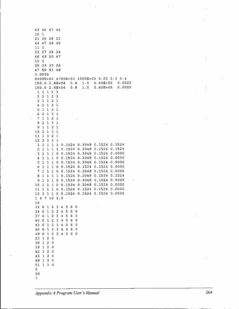
43 46 47 44 10 1 21 25 26 22 44 47 48 45 11 1 23 27 28 24 46 49 50 .47 12 1 25 29 30 26 47 50 51 48 0.0095 6400E+03 4700E+03 1500E+03 0.22 0.3 0.4 150 . 0 2 .8E+04 0.8 1. 5 0 40E+06 0 . 0025 150 . 0 2 .8E+04 0.8 1. 5 0 40E+06 0.0025
1 1 1 2 3 2 2 1 3 3 3 1 1 2 1 4 2 1 3 1 5 1 1 2 1 6 2 1 3 1 7 1 1 2 1 8 2 1 3 1 9 1 1 2 1
10 2 1 3 1 11 1 3 2 1 12 2 3 3 1
1 1 1 1 1 0 . 1524 0 3048 0 1524 0 1524 2 1 1 1 1 0 . 1524 0 3048 0 1524 0 1524 3 1 1 1 0 0 . 1524 0 3048 0 1524 0 0000 4 1 1 1 0 0 . 1524 0 3048 0 1524 0 0000 5 1 1 1 0 0 . 1524 0 3048 0 1524 0 0000 6 1 1 1 0 0 . 1524 0 1524 0 1524 0 0000 7 1 1 1 0 0 . 1524 0 3048 0 1524 0 0000 8 1 1 1 1 0 . 1524 0 3048 0 1524 0 1524 9 1 1 1 0 0 . 1524 0 3048 0 1524 0 0000
10 1 1 1 0 0 . 1524 0 3048 0 1524 0 0000 11 1 1 1 0 0 . 1524 0 1524 0 1524 0 0000 12 1 1 1 0 0 . 1524 0 1524 0 1524 0 0000 1 6 7 10 1 0 14 31 6 1 2 3 4 5 6 0 34 6 1 2 3 4 5 6 0 37 6 1 2 3 4 5 6 0 40 6 1 2 3 4 5 6 0 43 6 1 2 3 4 5 6 0 46 6 1 2 3 4 5 6 0 49 6 1 2 3 4 5 6 0 33 1 2 0 36 1 2 0 39 1 2 0 42 1 2 0 45 1 2 0 48 1 2 0 51 1 2 0 2 60
Appendix A Program User's Manual 264

33 0. 0 0 0 -7 6 1 3 36 0. 0 0 0 -7 6 1 3 39 0. 0 0 0 -7 6 1 3 42 0. 0 0 0 -7 6 1 3 45 0. 0 0 0 -7 6 1 3 48 0. 0 0 0 -7 6 1 3 51 0. 0 0 0 -7 6 1 3 0 33 1 0 001 33 1 2 4 4 0 0 2 0 0 0 0
3. Cyclic protocol file
This file contains three small cycles, three large cycles and one unidirectional push
over. The three small cycles have the same amplitude of 16 mm and the three large cycles
have the same amplitude of 32 mm. The final unidirectional push-over reaches 70 mm.
Another format can be used, in which one line represents one step:
400 0.001 0.0 0 0.002 0.0 0 0.003 0.0 0 0.004 0.0 0 0.005 0.0 0 0.006 0.0 0
14 0 .001 0 .015
-0.015 0 . 015
-0 . 015 0 . 015
-0.015 0 . 031
-0.031 0 . 031
-0,031 0.031
-0.031 0 . 001
0 .001 0 .001 0 .001 0 . 001 0 . 001 0 . 001 0 . 001 0 . 001 0 . 001 0 . 001 0 . 001 0 . 001 0 . 001 0 . 001
15 31 31 31 31 31 47 .63 63 63 63 63 31 69
Appendix A Program User's Manual 265

4. Time-acceleration history file
Format 1.
JOSHUA_jtest 1 1836 0.02D0 0.02D0 0.3D0 1.D0 1 0
0 . 057969329 -0 . 104540805 -0 . 161530065 -0 . 051302433
0 . 059312387 0.055029120
-0 . 183430398 -0 . 270305742
Format 2.
JOSHUA_jtest 1 1836 0.02D0 0.3D0 1.D0 1 0
0 200000E-01 0 579693E-01 0 300000E-01 -0 232857E-01 0 400000E-01 -0 104541E+00 0 600000E-01 -0 161530E+00 0 700000E-01 -0 106416E+00 0 800000E-01 -0 513024E-01 0 900000E-01 0 400498E-02 0 100000E+00 0 593124E-01 0 120000E+00 0 550291E-01 0 126667E+00 -0 244574E-01 0 133333E+00 -0 103944E+00 0 140000E+00 -0 183430E+00 0 160000E+00 -0 270306E+00
A.4.6. Examples of the output file of an eigensystem
This file gives the results of eigenvalues and eigenvectors of a system calculated by
LightFrame3D_Eigen. A total of 10 columns of eigenvectors (Only four of them are shown
here) are corresponding to the 10 eigenvalues. Each eigenvector contains the same rows as
the number of degrees of freedom of the system, from which one of the mode shapes can be
drawn. The a value for the mass-proportional damping at 5% damping ratio is also given.
Job t i t l e : box_open_24e_dy
Appendix A Program User's Manual 266
METHOD 1: SUBSPACE EIGENVALUES AND NATURAL FREQUENCIES
.58978E+03
.92801E+03
.48046E+04
. 77289E+04
.20081E+05
.23376E+05
.68356E+05
.12624E+06
. 14865E + 06
. 14891E + 06 EIGENVECTORS - . 39895E-04 -.74332E-04 -
. 00000E + 00 - . 16845E-05
.00000E+00
.00000E+00
. 00000E+00 - . 38529E-03 -.76884E-04 -
.00000E+00
.21235E-03
.00000E+00
.00000E+00
.00000E+00 -.83255E-04 -.70072E-05 •
.00000E+00 -.47372E-07
.00000E+00
.00000E+00
.00000E+00
.38651E+01
.48484E+01
. 11032E+02
. 13992E+.02
.22554E+02
.24333E+02
.41611E+02
.56547E+02
.61362E+02
.61416E+02
.26714E-05
.10784E-04
.00000E+00
.17431E-06
.00000E+00
.00000E+00
.00000E+00
.11307E-04
.12957E-04
.00000E+00
.73957E-03
.00000E+00
.00000E+00
.00000E+00
.54728E-05
.25562E-04
.00000E+00
.45783E-06
.00000E+00
.00000E+00
.00000E+00
-.77477E-04 -.13077E-03
.00000E+00 -.28189E-05
.00000E+00
.00000E+00
.00000E+00 -.71861E-03 -.13390E-03
.00000E+00 -.16717E-03
.00000E+00
.00000E+00
.00000E+00 -.16150E-03
.87966E-06
.00000E+00 -.62423E-07
.00000E+00
.00000E+00
.00000E+00
.20498E-05
.51672E-06
.00000E+00
.14615E-06
.00000E+00
.00000E+00
.00000E+00
. 83963E-06
. 80311E-06
. 00000E + 00
. 72696E-05
. 00000E + 00
.00000E+00
. 00000E+00
. 37452E-05
. 13786E-05
.00000E+00
.26904E-06
.00000E+00
. 00000E+00
.00000E+00
POSSIBLE ALFA AT 5% DAMPING RATIO IS
.24285E+01
A.5. Viewing graphic files generated by the postprocessor
Two files are generated by the postprocessor for visually displaying the deformed
shape of the structural system being analyzed. One is Defoshape.lsp, which presents the
structural mesh directly in AutoCAD software, and the other is Slides, scr, which is a script
file generated by the LightFrame3D program during its execution to create continuously
running slides showing the structural deformation step by step in both AutoCAD™ and MS
Powerpoint™ software.
Appendix A Program User's Manual 267
To run Defoshape.lsp, start A u t o C A D 1 M (R14 or later version). In the command line,
type: appload <Return>. When a window shows up, select and load Defoshape.lsp from the
working directory (The exact location of this file may vary for different Fortran compilers).
The deformation of the structural system being studied in all recorded steps wil l be displayed
on the screen.
To save slides generated by the LightFrame3D program, it is necessary to create a
directory as C:\slides. The slides are automatically saved in two formats. One format is the
AutoCAD™ slide format with suffix .sld, which is used for slide shows on the AutoCAD™
screen; and the other is the Windows™ metafile with suffix .WMF, which can be load by
many programs, for example, MS Powerpoint™. To present the slides on the AutoCAD™
screen, start AutoCAD™ (R14 or later version) and in the command line, type: script
<Return>. From the window, select and open file Slides.scr, which is in the working
directory. To run a slide show in MS Powerpoint™, start MS Powerpoint™, then use
command: "insert to load slides with suffix .WMF from directory C:\slides and save them
into a new file". Usually, creating a slide show in the Windows metafile format is more
convenient than doing that in the AutoCAD™ slide format (.sld), because MS Powerpoint™
is more commonly found on computers.
Appendix A Program User's Manual 268