numerical calculation of two-dimensional subsea cable

MATEMATIKA: MJIAM, Special Issue, December 2019, 15–32c© Penerbit UTM Press. All rights reserved

Numerical Calculation of Two-Dimensional Subsea Cable Tension

Problem Using Minimization Approach

1Nur Azira Jasman∗, 2Nur Adlin Lina Normisyidi, 3Yeak Sue Hoe,4Ahmad Razin Zainal Abidin and 5Mohd Ridza Mohd Haniffah1,3Department of Mathematical Sciences, Universiti Teknologi Malaysia

81310 UTM Johor Bahru, Malaysia2,4Department of Structure and Materials, Universiti Teknologi Malaysia

81310 UTM Johor Bahru, Malaysia5Department of Water and Environmental Engineering, Universiti Teknologi Malaysia

81310 UTM Johor Bahru, Malaysia

∗Corresponding author: [email protected]

Article historyReceived: 10 November 2019Received in revised form: 21 November 2019Accepted: 23 December 2019

Published online: 31 December 2019

Abstract Subsea cable laying is a risky and challenging operation faced by engineers,

due to many uncertainties arise during the operation. In order to ensure that subseacables are laid out diligently, the analysis of subsea cable tension during the laying

operation is crucial. This study focuses on the fatigue failure of cables that will causelarge hang-off loads based on catenary configuration after laying operation. The presented

problem was addressed using mathematical modelling with consideration for a number ofdefining parameters, which include external forces such as current velocity and design

parameters such as cable diameter. There were two types of subsea cable tension analysesstudied: tensional analysis of catenary configurations and tensional analysis of lazy waveconfigurations. The latter involved a buoyancy module that was incorporated in the

current catenary configuration that reduced subsea cable tension and enhanced subseacable lifespan. Both analyses were solved using minimization through the gradient-

based approach concerning on the tensional analysis of the subsea cable in differentconfigurations. Lazy wave configurations were shown to successfully reduce cable tension,

especially at the hang-off section.

Keywords Two-dimensional, Steady state problem, Catenary configuration, Lazy waveconfiguration, Minimization with gradient-based approach.

Mathematics Subject Classification 65D99, 65K05

1 Introduction

Subsea cable systems have been extensively used worldwide since the mid-19th century.Ever since subsea cable has played an important role in providing communications due to

Special Issue, December 2019 15–32 | www.matematika.utm.my | eISSN 0127-9602 |

Nur Azira Jasman et al. / MATEMATIKA Special Issue, December 2019, 15–32 16

their massive capacity, great reliability, and excellent communication quality. The rapid ofdevelopment of telecommunication systems has led to the exploitation of ocean environmentresources and the intensive deployment of subsea cables. During the subsea cable deploymentprocess, any incorrect manipulation scan cause unrepairable subsea cable damage. Therefore,the tension analysis of subsea cables has been explored by researcher over the past few decades.

Attention have been paid for the last few decades to theoretical studies about the staticand dynamic responses of subsea cables during the deployment process. Zajac [1] was the firstto develop a steady state theory for subsea cables in a typical deployment process in which themodel assumed as a straight line and excluded the effect of transient motions. Followed from thetheory developed by Zajac [1], many studies have considered different analysis approaches forboth static and dynamic subsea cable response [2-3]. After Zajac [1], Patel and Vaz [4] extendedthe steady state model into a two-dimensional model of transient subsea cable behavior in whichthe developed model was used to analyze cable top tension, required pay out rate as a function oftime, and cable configuration whenever a ship accelerates or decelerates. The two-dimensionalmodel was then extended into a three-dimensional model that considered the sheared currentseffect, subsea cable elastic deformation, and vessel speed during the laying process using theconventional finite element method and Runge-Kutta technique [5-10].

The numerical and experimental dynamic behavior results of subsea cables have been a greatinterest to the subsea cable design process. A comparison of the numerical and experimentalresults of this problem have been discussed in past studies in [11-14] in which subsea cablebending stiffness was calculated using the cable shape to determine where the cable experiencedthe greatest stress and thrust from the laying ship. A recent study by Han et al. [15] establisheda mathematical model in which the initial-boundary value problem was addressed using aPartial Differential Equation (PDE). These mathematical models have been used to describethe three-dimensional motion of subsea cables being laid onto the seabed of varying depths.

Subsea cable installation is an extremely important lifetime process that requires very precisecontrol. One of the challenges faced during subsea cable deployment is slack formation asstated by Abidin et al. [16]. Slack formed during the subsea cable laying process increasesthe possibility of the cable being laid too long for planed route,causing a buckling issue at thetouchdown point (TDP). According to Wang et al. [17], the configuration and performance ofsubsea cables are essential to subsea cable installation. A free hanging subsea cable hangs froma floating production vessel to the seabed, forming a catenary shape has a lower manufacturingcost and good ability to resist high temperature. However, this kind of configuration may facebuckling issues at the touchdown zone. Variations in catenary configurations were developedconsidering the existence of buoyancy modules, which are a logical extension of the catenaryshape. These new variations in catenary configurations were modeled by installing buoyancymodules into subsea cables at a certain part to eliminate partial tension. According to Wangand Duan [18], buoyancy modules equipped onto subsea cables tend to decouple catenaryconfigurations from surface dynamics in the touchdown region, which ensures that the strength,fatigue performance, and platform payload of the cable are within acceptable limits.

In summary, most studies have mainly focused on subsea cables without buoyancy modulesto allow for simple and easy subsea cable installation. Hence, this study extends the formulatedmathematical model by including buoyancy modules to provide insight into subsea cablescatenary configurations, which are very sensitive to fatigue and have a high top tension. Theimplementation of buoyancy modules onto subsea cables in past studies only focused on the


pipeline itself to show the buoyancy modules ability to reduce tension along the pipeline. Thus,this study was conducted to provide insight into the work ability of buoyancy modules onsubsea cables as both subsea cables and pipelines are slender structures subject to the similaraccidental impact loads with different local damage mechanisms due to the discrepancies incable diameter, structural configuration, and flexural rigidity.

The problem considered in this study considered subsea cables in the (1) catenaryconfiguration, and (2) lazy wave configuration. The study theory was formulated and usedto solve problems related to subsea cable tension analysis in engineering applications. In thisstudy, subsea cable tension analysis was based on the following assumptions:

• Continuity: Subsea cables were considered continuous in terms of tension and forceanalysis

• Flexibility: Bending stiffness was neglected, and bending was only considered exceptmomentarily at the sea surface node of the top boundary condition

• The subsea cable was assumed to be fully immersed in sea water

• The drag coefficient (CD), lift coefficient (CL), water density (ρw), and cable density (ρc)were considered constant.

2 Theoretical Model

The first model formulated in this paper was based on subsea cables in catenary configurations.The aim of this model was to analyze the position of maximum tension on the subsea cableduring its practical installation in a steady state condition. This model was further enhancedby the installation of a buoyancy module on certain parts of the subsea cable to create a lazywave configuration.

2.1 Equilibrium Equations for the Subsea Cable in Water

The model formulated in this study was based on the Cartesian coordinate system. Thispaper established a two-dimensional subsea cable mathematical model that considered oceanenvironmental effects such as lift force, drag force, and ocean current for steady state cases.When a subsea cable is laid from the floating production vessel to the TDP, the componentsthat contribute to the tensional forces (T ) along the subsea cable can be described as:

• Gravity force (W∆s), which is due to subsea cable self-weight

• Buoyancy force (B), which is equal to the weight of its displaced fluid

• Drag force (D), which is the force a flowing fluid exerts on a body in the flow direction

• Lift force (L), which is the force a flowing fluid exerts on a body in the normal flowdirection

Considering a cable length as an infinitesimal element, with a leftward ∆s and water flowdirection, the possible forces acting on a subsea cable in water is illustrated in Figure 1.


Figure 1: Forces Acting on The Subsea Cable in Water Per Element.

2.2 Mathematical Model of Subsea Cables in Catenary Configurations

Catenary shape of subsea cables can be described as a free hanging subsea cable without abuoyancy module hanging from a floating production vessel to the seabed. It has become apopular configuration for the deployment of subsea cables near platforms as it is a low costalternative to subsea cable design.

In steady state conditions, the subsea cable is considered to be laid onto the seabed andthe last point of the cable touching the seabed is known as the touchdown point (TDP), whichis fixed in place. The TDP is the initial point from which the length of the subsea cable ismeasured to the floating production vessel. The parameter, s (arc length) was introduced todenote the length of the subsea cable. The study model does not consider the sea surface effect(wave) on the subsea cable.

Based on the Cartesian coordinate system, the cable laying ship starts at origin, o. Theship sails and lays the subsea cable from point P along the prescribed lines. The arc length,s is introduced to denote the length of the cable from point P to any point until the desiredcable configuration is achieved. Figure 2 illustrate a subsea cable in a catenary configuration.Based on Figure 2, Vx is the velocity of water (current velocity) and H is the water depth.

Figure 2: Illustration of Subsea Cable in Catenary Configuration.


The two-dimensional subsea cable steady state model was derived based on some physical andmechanical subsea cable laws. This study’s notations are described as follows:

r - The radius of subsea cable, where d = 2r is the diameter of subsea cable.g - Gravitational acceleration.W - Self-weight of a cable per unit length in water.Txi

(s) - Tension force at ith point in the x-direction.Tyi

(s) - Tension force at ith point in the y-direction.ρc - Density of subsea cable.ρw - Density of seawater.ρg∆s - Gravity of cable segment ∆s, ρ = πr2ρc.ρog∆s - Buoyancy of cable segment ∆s, ρo = πr2ρw.Dx - Drag force of seawater in the x-direction.Dy - Drag force of seawater in the y-direction.Lx - Lift force of seawater in the x-direction.Ly - Drag force of seawater in the y-direction.

Generally, the drag force, D and lift force, L were obtained when the upstream velocity (relativeto body) of fluid, V and fluid density, ρf were measured using flow over body using Equation(1) and (2), respectively.

D = CD

ρf

2V 2Ap (1)

L = CL

ρf

2V 2A (2)

CD in Equation (1) denote the total drag coefficient while CL in Equation (2) is the total liftforce. Ap is the frontal area which means the projected area seen by a person looking toward theobject from a direction parallel to the upstream velocity V and variable A is the planform areaseen by a person looking toward the object from a direction normal to the upstream velocityV .

In this study, the water velocity along the y-direction was neglected as it is very smallin the ocean where vy (x, y) = 0. Water velocity along the x-direction was written as vx =

Vx(x, y)~m = (Ux, Uy) was the velocity of the cable segment relative to the water while ~̀ was a

vector of ~̀ = (∆x, ∆y). The drag and lift force in the x-direction and y-direction were defined

using Equation (3) and (4) respectively considering the vector of ~m and ~̀.

Dxi= −KDUxi

∣

∣

∣

~̀i × ~mi

∣

∣

∣

Dyi= −KDUyi

∣

∣

∣

~̀i × ~mi

∣

∣

∣

(3)

Lxi= KLU

∣

∣

∣

~̀i · ~mi

∣

∣

∣

E(1,0)P sgn

(

~̀i · ~mi

)

Lyi= KLU

∣

∣

∣

~̀i · ~mi

∣

∣

∣

E(0,1)P sgn

(

~̀i · ~mi

)

(4)


where the KD and and KL used in Equations (3) and (4) were drag and lift coefficient definedusing Equations (5) and (6) respectively, while parameter E (a, b) was defined using Equation(7)

KD = CD

ρw

2d (5)

KL = CL

ρw

2d (6)

E (a, b)(

U2 − aU2xi− bU2

yi

)

(

a∂x

∂s+ b

∂y

∂s

)

−

[

(1− a)Uxi

∂x

∂s+ (1 − b)Uyi

∂y

∂s

]

(aUxi+ bUyi

) (7)

The direction of the drag and lift forces with respect to the direction of the upstream velocity,V is illustrated in Figure 3.

(a) Direction of Force if ~̀i·~mi ≥ 0

(b) Direction of Force if ~̀i·~mi < 0

Figure 3: Direction of Force with Respect to Upstream Velocities.

The equilibrium equation of a subsea cable in catenary configuration for steady state casesin x-direction and y-direction can be given by Equations (8) and (9) respectively.

Txi+1 cos αi+1 + Txicos αi + Dxi

+ Lxi= 0 (8)

Tyicosβi + Tyi+1 cosβi+1 + Dyi

+ Lyi+ W∆si = 0 (9)

where the angle calculation for the subsea cable elements α(s) and β(s) were obtained by

considering the dot product between vector ~T ,~i, and/or ~j as given in Equation (10).


~Ti ·~i =∣

∣

∣

~Ti

∣

∣

∣

∣

∣

∣

~i∣

∣

∣cos αi,

~Ti ·~j =∣

∣

∣

~Ti

∣

∣

∣

∣

∣

∣

~j∣

∣

∣cosβi,

~Ti+1 ·~i =∣

∣

∣

~Ti+1

∣

∣

∣

∣

∣

∣

~i∣

∣

∣cos αi+1,

~Ti+1 ·~j =∣

∣

∣

~Ti+1

∣

∣

∣

∣

∣

∣

~j∣

∣

∣cos βi+1.

(10)

2.2.1 Boundary Conditions for Subsea Cable Problem in Catenary Configuration

Boundary conditions for subsea cable are important to the analysis process. In this paper,subsea cable were modelled by discretizing them into smaller elements as shown in Figure 4.

Figure 4: Subsea Cable Segment Division.

Based on Figure 4, (x1, y1) denotes TDP and the boundary condition at this point is basedon a single moment of balance at the hanging point in the floating production vessel. Thiscondition was considered as the subsea cable was assumed to have the properties of a rigid bodyelement. The equilibrium force was considered in the clockwise and anti-clockwise directionusing Equation (11) and (12), respectively.

Force in anti-clockwise rotationW · ∆si · rxi

(11)

Force in clockwise rotationForce · Ry (12)

By combining both Equations (11) and (12), while considering drag and lift force, theequilibrium force at TDP from a single moment at sea surface node can be given as Equation(13).


Ns∑

i=1

(W · ∆si · rxi+ Dxi

· ryi+ Lyi

· rxi) = Force · Ry,

F orce =

Ns∑

i=1


· ryi+ Lyi

· rxi)

Ry.

(13)

Boundary condition at TDP can be said as equal to the Force obtained from a single momentat sea surface node (T1 = Force). The boundary condition at the top node was obtained byprojecting the force into the x-direction and y-direction. Total force at the top subsea cablenode was described by Equations (14) and (15). T̄1 in equation (14) denotes the tension atTDP, which was calculated using the the total force based on a single moment at sea surfacepoint.

TxNscosαNs = T̄1 (14)

TyNscos βNs =

Ns∑

2

(W∆si + Lyi) (15)

The input data in this study are tabulated as in Table 1. The parameter values were only formathematical simulation and were not used as a benchmark for any actual problem.

Table 1: Input Data

Parameter Value

Diameter of cable, d 0.023 m

Water depth, H 80 m

Density of cable, ρc 2888 kg/m3

Density of water. ρw 1024.8103 kg/m3

Cable weight in water, W(

π(

d2

)2(ρc − ρw) g

)

kg/ms2

Drag coefficient, CD 1.2

Lift coefficient, CL 0.024

Gravity, g 9.8 m/s2

Relative velocity, V 1.2 m/s

2.3 Mathematical Model for Subsea Cables in a Lazy Wave Configuration

The second model was based on subsea cable in a lazy wave configuration. This model wasdeveloped to reduce slack formation and improve fatigue performance in subsea cable designsin catenary configuration. The model considered in this case illustrated in Figure 5.


Figure 5: Illustration of Subsea Cables with Buoyancy Modules

This mathematical model for subsea cables was obtained by extending the formulationobtained for catenary problem. The equilibrium equation in y-direction was modified to considerthe buoyancy force to the left and right region of the buoyancy module as illustrated in Figure5. The equilibrium equation related to the x-direction was obtained directly from Equation(8). The equilibrium equation for subsea cables with buoyancy module in a two-dimensionalsteady state can be written in the x-direction and y-direction using Equation (16) and (17)respectively.

x−directionTxi+1 cos αi+1 + Txi

cos αi + Dxi+ Lyi

= 0 (16)

y−direction

Tyicosβi + Tyi+1 cosβi+1 + Dyi

+ Lyi+ W∆si = 0

• Left element of the buoyancy module

Ti cos βi +

Left element of

buoyancy module∑

i=1

(W∆si + Lyi) = 0 (17)

• Right element of the buoyancy module

Ti+1 cos βi+1 +

Right element of

buoyancy module∑

i=1

(W∆si + Lyi) = 0

• At the buoyancy module point

Ti cos βi + Ti+1 cosβi+1 − Fbm = 0


Note that the equilibrium equation at the buoyancy module point in Equation (17) wasformulated to determine the buoyancy force of the buoyancy module. The buoyancy force of thebuoyancy module was calculated considering the subsea cable element in which we proposed toimplement the buoyancy module. The equation for calculating the buoyancy force of buoyancymodule was written using Equation (18), where p denotes the desired buoyancy module weightpercentage that will balance the buoyancy module in certain conditions while L denotes thelength of the buoyancy module region.

Buoyancy Force of the buoyancy module, Fbm = L · p (18)

Boundary conditions for this problem were also based on the theory developed for thecatenary configuration with slight modifications.

2.3.1 Boundary Conditions for Subsea Cable in Lazy Wave Configurations

The subsea cable configuration with a buoyancy module was created using an interpolationtechnique that discretized the subsea cable into N segments. For the boundary conditionat TDP, Equation (13) was considered but the calculation was made based on the buoyancymodule region illustrated in Figure 5 to produce Equation (19).

Buoyancy

Node∑

i=1


· ryi+ Lyi

· rxi) = Force · Ry,

F orce =

Buoyancy

Node∑

i=1


· ryi+ Lyi

· rxi)

Ry.

(19)

Next, the boundary condition at the top node was calculated using Equations (14) and (15)but the calculations were only made on the floating production vessel region as shown in Figure5. The equation for the boundary condition at the top node was calculated using Equations(20) and (21) in the x-direction and y-direction respectively.

TxNscosαNs = T̄1 (20)

TyNscos βNs =

Ns∑

Floating

Production

V essel

(W∆si + Lyi) (21)

The data considered for this case shown in Table 1. The effectiveness of the new formulatedmathematical model in steady state condition was validated and compared with previousstudies. A comparison between present and previous model was made using subsea cable tensionanalysis and cable configurations based on different parameters such as cable weight and cablediameter. The cable configuration of this study was similar to Yang et al. [13]. A comparisonof subsea cable tension analysis between this study and previous study showed good agreement


for performance measurements such as cable diameter, water depth and current velocity. Theformulated mathematical subsea cable model in a catenary configurations was then extendedthrough the addition of buoyancy module. The results of both models are discussed in the nextsection.

3 Results and Discussion

The mathematical subsea cable model in this study was developed based on Yang et al. [13]and Han et al. [15]. The formulated model was updated with appropriate boundary conditions.To show the validity of the model, comparisons between the developed model and Yang et al.[13] were conducted as shown in the next section.

3.1 Comparison of Subsea Cable Tension with Past Study

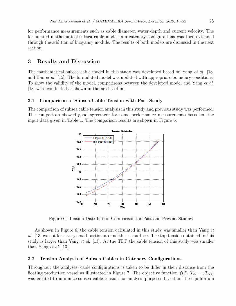
The comparison of subsea cable tension analysis in this study and previous study was performed.The comparison showed good agreement for some performance measurements based on theinput data given in Table 1. The comparison results are shown in Figure 6.

Figure 6: Tension Distribution Comparison for Past and Present Studies

As shown in Figure 6, the cable tension calculated in this study was smaller than Yang etal. [13] except for a very small portion around the sea surface. The top tension obtained in thisstudy is larger than Yang et al. [13]. At the TDP the cable tension of this study was smallerthan Yang et al. [13].

3.2 Tension Analysis of Subsea Cables in Catenary Configurations

Throughout the analyses, cable configurations is taken to be differ in their distance from thefloating production vessel as illustrated in Figure 7. The objective function f(T1, T2, . . . , TNs)was created to minimize subsea cable tension for analysis purposes based on the equilibrium


equation obtained in Equations (8) and (9) as well as boundary conditions of Equations (13)to (15) Table 2 shows the corresponding tensions in each cable element. The objective functionwas written as follows:

Let

netFy =Ns∑

i=2

(W∆si + Lyi)

x−direction

f = f +Ns−1∑

i=2

(

Txi+1cos αxi+1

+ Txicos αxi

+ Dxi+ Lxi

)2

y−direction

f = f +Ns−1∑

i=2

(

Tyicosβyi

+ Tyi+1cosβyi+1

+ +Dyi+ Lyi

+ W∆si

)2

Boundary condition at TDP

f = f +(

T̄1 − Force)2

Boundary condition at top node

f = f +(

Ti cosαi − ~T1

)2

+ (Ti cos βi − netFy)2

Figure 7: Cable Configuration of Different Distances from The Floating Production Vessel


Table 2: Tension Distribution Along Subsea Cables in Catenary Configurations (Starts fromTDP)

For each configuration, tension increases from TDP to its maximum value at the hangingpoint. This is due to a gravitational effect in which the cable element at the TDP is restinghorizontally on the seabed while the cable elements near the hanging point does not havesupport and has to withstand the weight of the cables below. For the cable length in the x-direction of 60m, it can be seen clearly in Table 2 that the tension distribution for the subseacable reached more than 500N. Apart from this, the longer the cable, the higher the tensionat hanging point for each cable. In order to reduce cable tension, a support is needed such asa buoyancy module which will create a lazy wave configuration that will reduce the extremestresses and fatigue of the subsea cable to within an acceptable limit.

3.3 Tension Analysis of Subsea Cables for Lazy Wave Configurations

The tension analysis of subsea cables with a lazy wave configuration problem were based onEquations (16) and (17). The cable configuration for this case was created based on severaldifferent buoyancy module distances from the seabed (30m, 40m and 50m) and from the floatingproduction vessel (20m, 30m and 40m). Note that the x-distance of the cable length was fixedat 60m, so it could be compared to the last column of Table 2 for subsea cable configurationswithout a buoyancy module. The objective function f(T1, T2, . . . , TNs) was created based onthe equilibrium equation obtained in Equations (16), (17), (19), (20) and (21).


3.3.1 Tension Analysis of Subsea Cables with Buoyancy Module 30m from Seabed

The buoyancy module was installed 30m from the seabed illustrated in Figure 8, with differentdistances from the floating production vessel of 20m, 30m and 40m respectively.

(a) (b) (c)

Figure 8: Cable Configuration with Buoyancy Module 30m from Seabed (a)20m, (b)30m and(c)40m distance from floating Production Vessel

Table 3: Tension Distribution Along Subsea Cables With Buoyancy Module 30m from SeabedWith Varying Distances from the Floating Production Vessel.

Table 3 shows the corresponding tensions in each cable element. The buoyancy module pointwas outlined by a black color in Table 3. All the results had an appropriate tension distributionalong the subsea cable that did not exceed the critical value of 500N.


3.3.2 Tension Analysis of Subsea Cables with Buoyancy Module 40m from Seabed

This section discusses on the results for the buoyancy module 40m from the seabed which areshown in Figure 9 with a distance from the floating production vessel of 20m, 30m and 40mrespectively.

(a) (b) (c)

Figure 9: Cable Configuration with Buoyancy Module 40m from Seabed (a)20m, (b)30m and(c)40m distance from floating Production Vessel.

Table 4: Tension Distribution Along Subsea Cable With Buoyancy Module 40m from SeabedWith Varying Distances from Floating Production Vessel

The buoyancy module point was outlined using a black color in Table 4. The cableconfiguration with buoyancy module position of 30m or 40m from the floating productionvessel also had an appropriate tension distribution along the subsea cable less than 500N.


3.3.3 Tension Analysis of Subsea Cable with Buoyancy Module 50m from Seabed

This section discusses the results for the buoyancy module 50m from the seabed as shown inFigure 10 with different distances from the floating production vessel of 20m, 30m and 40mrespectively.

(a) (b) (c)

Figure 10: Cable Configuration with Buoyancy Module 50m from Seabed (a)20m, (b)30m and(c)40m distance from floating Production Vessel.

Table 5: Tension Distribution Along Subsea Cable With Buoyancy Module of 50m fromSeabed With Varying Distances from Floating Production Vessel

The buoyancy module point was outlined by using a black color in Table 5. Based on thethree models, only cable configurations with a buoyancy module position 40m from the floatingproduction vessel had an appropriate tension distribution along the subsea cable that was lessthan 500N.


4 Conclusion and Recommendations

Mathematical models of subsea cable for both catenary and lazy wave configurations weregenerated with assumption that velocity was constant, the seabed was flat, and the effects ofwind and waves were insignificant. Two solutions were presented in this paper: tension analysisfor subsea cables without buoyancy modules (catenary configuration), and tension analysis forsubsea cables with buoyancy modules (lazy wave configuration). Both solutions used the sameunconstrained minimization approach. It can be seen clearly in the report that the tensiondistribution for subsea cables in the catenary configuration was greater than 500N, which willcause a large hang-off load at the floating production vessel.

Buoyancy modules were installed in a suitable section of the catenary cable shape, forming alazy wave configuration that reduced the tension of the subsea cable at the floating productionvessel. From the nine different buoyancy module positions, the best buoyancy module positionwas 30m from the seabed and 30m from the vessel because its tension distribution was thelowest and was below the acceptable limit of 500N. Moreover, the buoyancy force used forthis configuration was also smaller than other configurations. The proposed buoyancy moduleshould have a buoyancy force percentage within 40% of the total subsea cable weight.

In future research, this study suggests researchers to investigate more reliable lazy waveconfigurations since different shapes will produce different amounts of tension along the subseacable. Subsea cable configurations should be developed based on different criteria such asdifferent buoyancy force, buoyancy module distance from the seabed, and buoyancy moduledistances from the floating production vessel.

Acknowledgement

The authors would like to express gratitude to the Ministry of Higher Education Malaysia fortheir financial support through MyBrainSc Scholarship throughout study period.

References

[1] Zajac, E. Dynamics and kinematics of the laying and recovery of submarine cable. TheBell System Technical Journal. 1957. 36(5): 1129-1207.

[2] Yoshizawa, N. and Yabuta, T. Study on submarine cable tension during laying. IEEEJournal of Oceanic Engineering. 1983. 8(4): 293-299.

[3] Burgess, J. Modelling of undersea cable installation with a finite difference method. Paperpresented at the The First International Offshore and Polar Engineering Conference. 1991.

[4] Patel, M. and Vaz, M. The transient behaviour of marine cables being laid—the two-dimensional problem. Applied Ocean Research. 1995. 17(4): 245-258.

[5] Vaz, M., Witz, J. and Patel, M. Three dimensional transient analysis of the installation ofmarine cables. Acta Mechanica. 1997. 124(1-4): 1-26.

[6] Vaz, M. and Patel, M. Three-dimensional behaviour of elastic marine cables in shearedcurrents. Applied Ocean Research. 2000. 22(1): 45-53.


[7] Chucheepsakul, S., Srinil, N. and Petchpeart, P. A variational approach for three-dimensional model of extensible marine cables with specified top tension. AppliedMathematical Modelling. 2003. 27(10): 781-803.

[8] Wang, F., Huang, G.-l. and Deng, D.-h. Steady state analysis of towed marine cables.Journal of Shangsai Jiatong University (Science) 2008. 13(2): 239-244.

[9] Wang, Y., Bian, X., Zhang, X. and Xie, W. A study on the influence of cable tensionon the movement of cable laying ship. Paper presented at the OCEANS 2010 MTS/IEEESEATTLE. 2010.

[10] Yang, N. and Jeng, D.-S. Three-dimensional Analysis of Elastic Marine Cable duringLaying. Paper presented at the The Eleventh ISOPE Pacific/Asia Offshore MechanicsSymposium. 2014.

[11] Dreyer, T. and Van Vuuren, J. H. A comparison between continuous and discrete modellingof cables with bending stiffness. Applied Mathematical Modelling. 1999. 23(7): 527-541.

[12] Park, H., Jung, D. and Koterayama, W. A numerical and experimental study on dynamicsof a towed low tension cable. Applied Ocean Research. 2003. 5(5): 289-299.

[13] Howison, S. Practical Applied Mathematics: Modelling, Analysis, Approximation.Cambridge University Press. 2005.

[14] Yang, N., Jeng, D. and Zhou, X. Tension analysis of submarine cables during layingoperations. Open Civ. Eng. J. 2013. 7(1): 282-291.

[15] Han, H., Li, X. and Zhou, H.-S. 3D mathematical model and numerical simulation forlaying marine cable along prescribed trajectory on seabed. Applied Mathematical Modelling2018. 60: 94-111.

[16] Abidin, A. R. Z., Mustafa, S., Aziz, Z. A. and Ismail, K. Subsea Cable Laying Problem.Matematika. 2018. 34(2): 173-186.

[17] Wang, J., Duan, M., Fan, J. and Liu, Y. Static equilibrium configuration of deepwatersteel lazy-wave riser. Paper presented at the The Twenty-third International Offshore andPolar Engineering Conference. 2013.

[18] Wang, J. and Duan, M. A nonlinear model for deepwater steel lazy-wave riser configurationwith ocean current and internal flow. Ocean Engineering. 2015. 94: 155-162.

numerical calculation of two-dimensional subsea cable

Documents