ntrs.nasa.gov · on the convergence of an iterative formulation of the electromagnetic scattering...
TRANSCRIPT
' 0? kN
•?»*£?$'
https://ntrs.nasa.gov/search.jsp?R=19860018044 2018-08-04T19:28:19+00:00Z
ON THE CONVERGENCE OF AN ITERATIVE FORMULATION
OF THE ELECTROMAGNETIC SCATTERING
FROM AN INFINITE GRATING OF THIN NIRES
by
JERRY C. BRAND
DEPARTMENT OF ELECTRICAL AND COMPUTER ENGINEERING
NORTH CAROLINA STATE UNIVERSITY*
Raleigh, North Carolina
May 1985
This research was supported by the National Aeronautics and SpaceAdministration through grant NSG 1588.
ABSTRACT
Contraction theory is applied to an iterative formulation
of electromagnetic scattering from periodic structures and a
computational method for insuring convergence is developed. A
short history of spectral (or k-space) formulation is presented
with an emphasis on application to periodic surfaces. The
mathematical background for formulating an iterative equation
is covered using straightforward single variable examples
including an extension to vector spaces. To insure a
convergent solution of the iterative equation, a process called
the contraction corrector method is developed. Convergence
properties of previously presented iterative solutions to
one-dimensional problems are examined utilizing contraction
theory and the general conditions for achieving a convergent
solution are explored. The contraction corrector method is
then applied to several scattering problems including an
infinite grating of thin wires with the solution data compared
to previous works. Problems associated with extending the
contraction corrector method to two-dimensional iterative
formulations are outlined including the benefits of applying
this process to difficult practical problems such as knitted
mesh surfaces.

Ill
ACKNOWLEDGEMENTS
The author wishes to thank all the people who have
helped him in the completion of his graduate work. In par-
ticular, he expresses deepest appreciation to his major ad-
visor, Professor J. Frank Kauffman, who was first a friend
and then a mentor in many situations. Special thanks are
extended to the people in the RF Subsystems Section for the
support they offered, and especially to Linda Snyder and
Susan Sanders for their help in typing.
The author also wishes to express his thanks to his
wife who gave so much support in the completion of this
dissertation and for the final typing of the dissertation.
IVTABLE OF CONTENTS
Page
LIST OF TABLES v
LIST OF FIGURES vi
I. INTRODUCTION 1
II. REVIEW OF THE FUNDAMENTAL FORMULATION 4
III. MATHEMATICAL FORMULATION OF ITERATIVE
EQUATIONS, CONTRACTIONS AND FIXED-
POINT THEORY 12
IV. THE PERIODIC STRUCTURE: ' A CANONICAL
CASE AND THE REGIONS OF SOLVABILITY 23
V. THE PROBLEM OF AN INFINITE GRATING OF
THIN WIRES 48
VI. EXTENSION TO TWO-DIMENSIONAL PROBLEMS 61
VII. CONCLUSIONS 74
REFERENCES . 76
APPENDIX A 79
APPENDIX B .' 86
APPENDIX C 90
LIST OF TABLES
Page
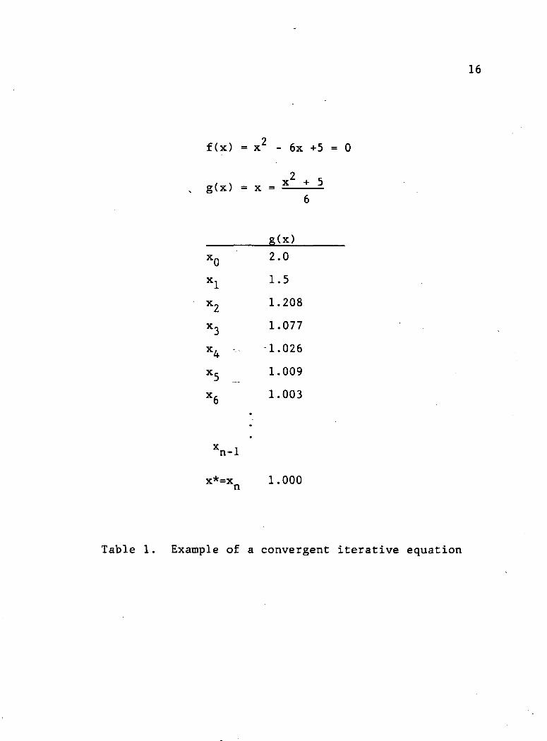
Table 1. Example of a convergent iterative
equation 16
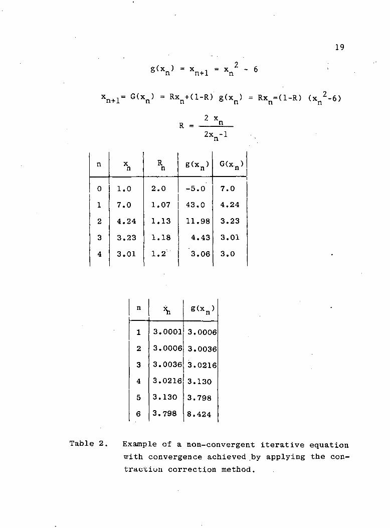
Table 2. Example of a non-convergent iterative
equation with convergence achieved by
applying the contraction corrector
method 19
Table 3. Example of a complex valued iterative
equation and the use of a complex con-
traction corrector o 21
Table 4. Example of a two-variable contraction
corrector method 67
LIST OF FIGURESVI
Page
Figure 1. a) The planar periodic surface indi-
cating electric current density
J over the conducting portion
and K over the aperture portionmn
b) Unit cell definition ... o .... g
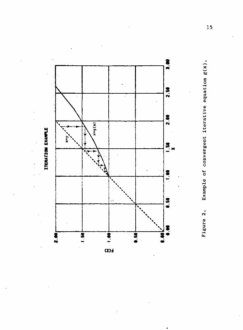
Figure 2. Example of convergent iterative equa-
tion g(x) 15
Figure 3. Free-standing conducting strips with
Floquet cell width a, aperture size
b and conductivity a 32
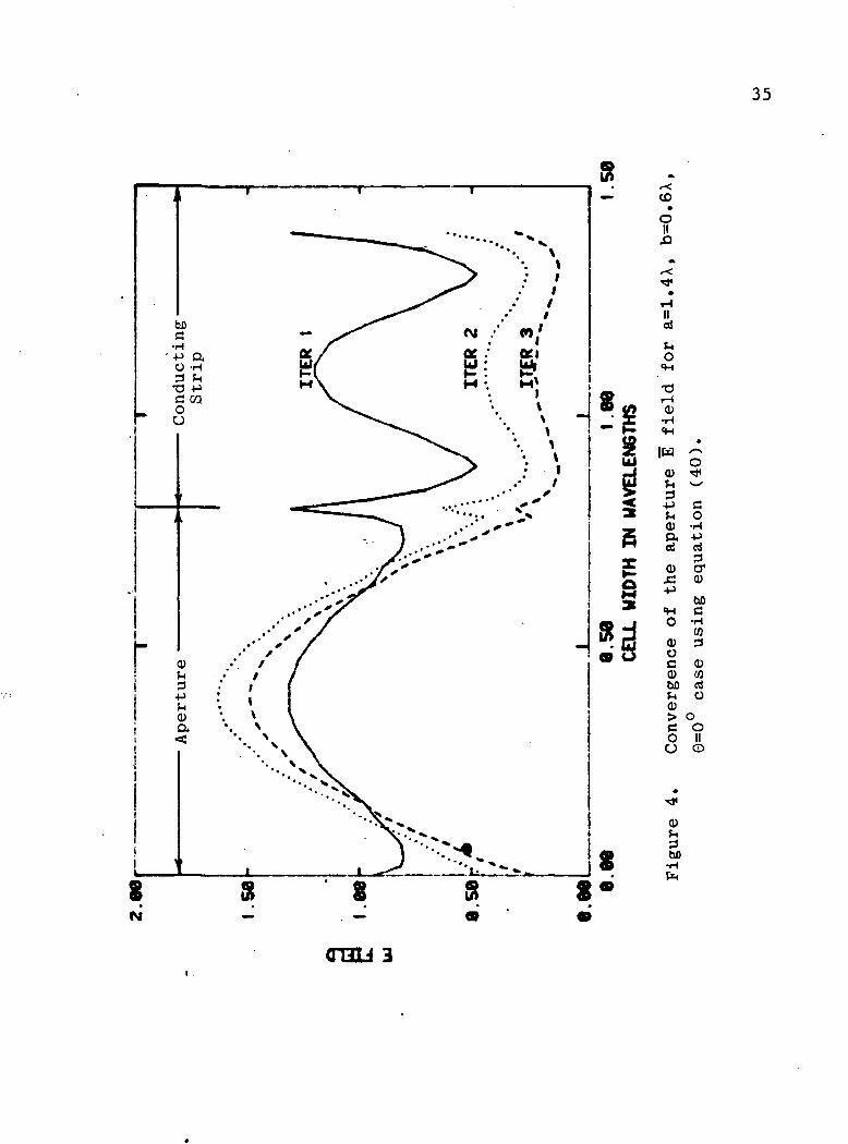
Figure 4. Convergence of the aperture E field
for a=1.4X, b=0.6X, 6=0* case using
equation (40) 35
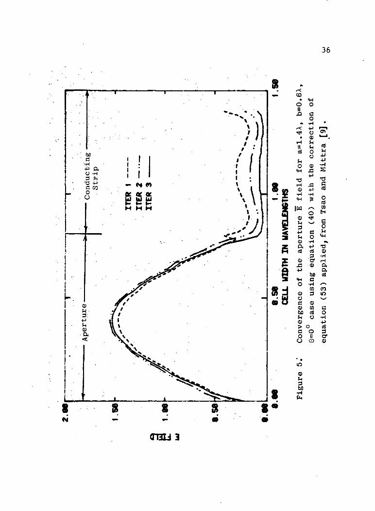
Figure 5. Convergence of the aperture E field
for a=1.4X, b=0.6X, 0=0° case using
equation (40) with the correction of
equation (53) applied/ from Tsao and
Mittra IB] 36
Figure 6. Convergence of the aperture E field
for a=1.4X, b=0.6A» 9=0° case using
equation (42). This is the contrac-
tion corrector method 38
Figure 7. Contraction factor for a cell width of
1.4X, incidence angle 0=0° with H-wave39
polarization and <*>=0°
vii
Page
Figure 8. Contraction factor for a strip width of
0.6x, incidence angle 0=0° with H-wave
polarization and $=0° .......... 40
Figure 9. Contraction factor for a strip width of
0.1X, incidence angle of 0=0° with
H-wave polarization and $=0° . . . . . . ' • 42
Figure 10. Convergence survey using contraction
criteria for 0°<0<90°, $=0°, a=0.9X,
and b=0.4X. .... ........... 43
Figure 11. a) Non-convergent results of the vari-
ational corrected iterative equation
for 0=70° ........ . . . . . . 45
b) Non-convergent results for the basic
iterative equation with 0=70° .... ^g
Figure 12. Convergent results obtained from the
contraction corrector method of equation
(30) with "5=0°, 0=70°, a=1.4X and
b=0.6A .............. ....
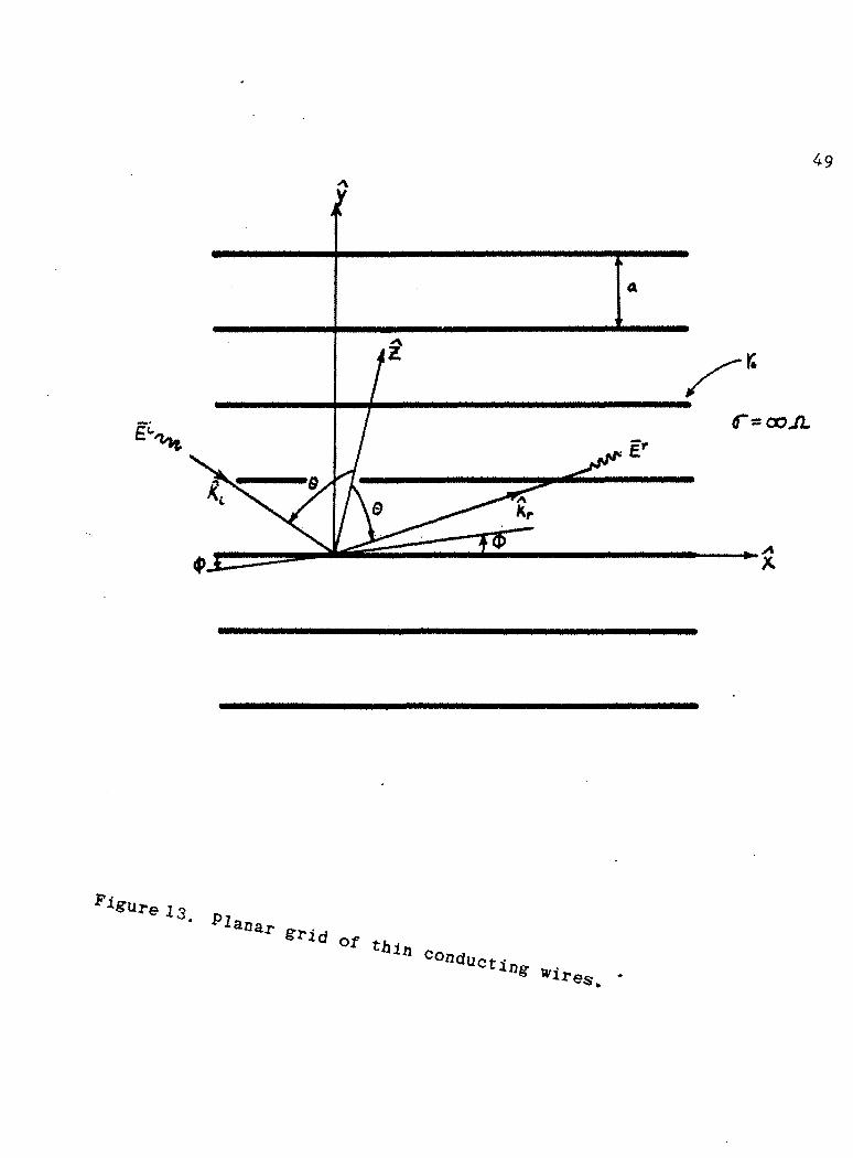
Figure 13. Planar grid of thin conducting wires. . . 49
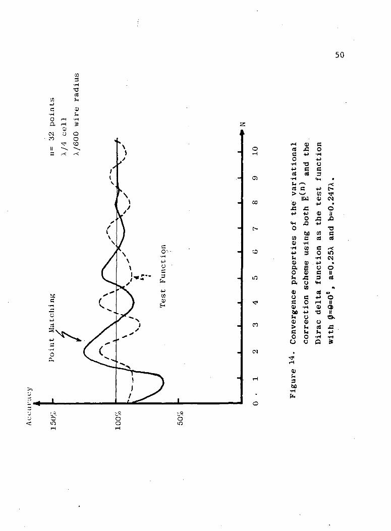
Figure 14. Convergence properties of the variation-
al correction scheme using both E^ ' and
the Dirac delta function as the test
function with 0=$=0°, a=0.25X and
b=0.247X ................. 50
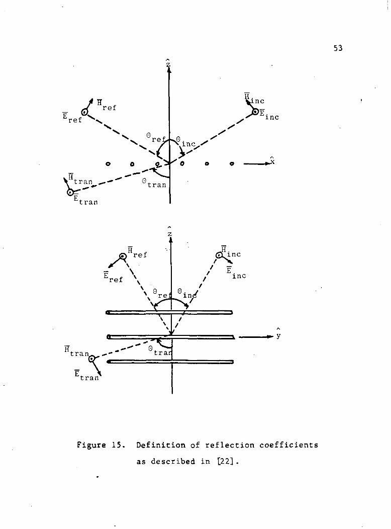
Figure 15. Definition of reflection coefficients as
described in [22l ............ 53
viii
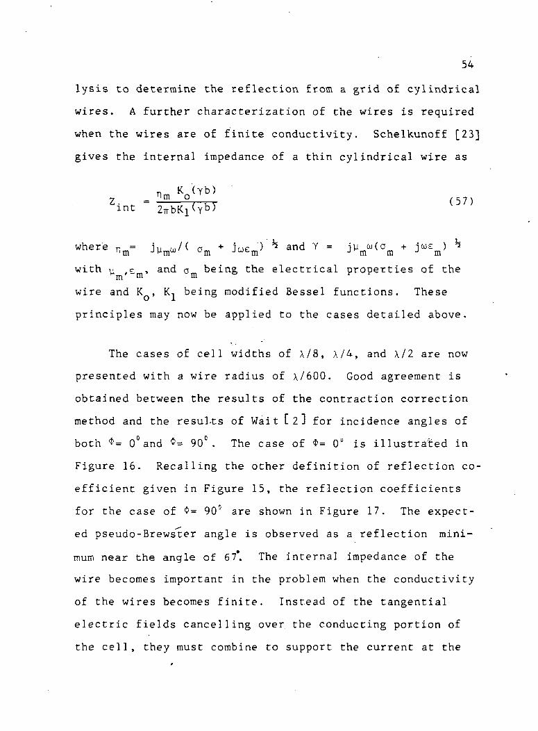
PageFigure 16. Comparison of results obtained from Wait(2j
and equation (30) for various cell widths
with <J>=0° , 0<G< 90°, and o= « S 55
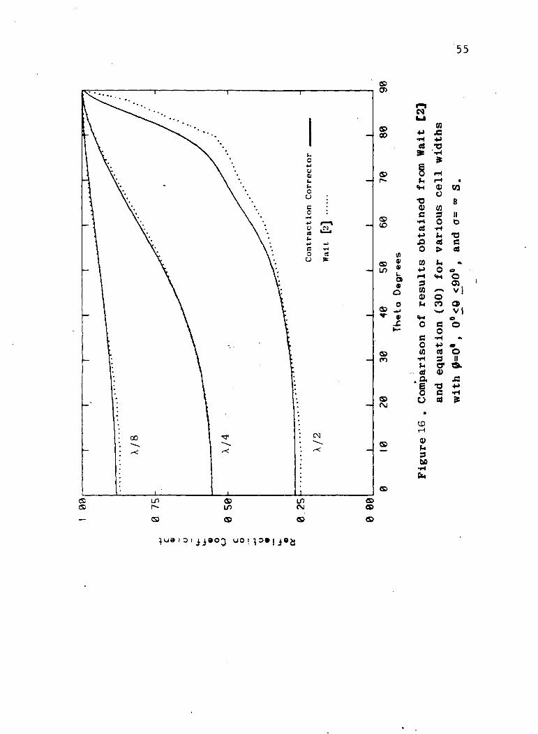
Figure 17. Reflection coefficient as defined in
Figure 15 for $=90°, 0°<0<90°, a=0.247X
and a=°°S
Figure 18. Several cases of finite conductivity
with 0=0°, 0°<G<90°, a=0.25X and
b=0.247X ................. 58
Figure 19. Illustration of converged accuracy for
various number of terms with a=0.25A,
b=0.247X, 0=$=0° and a= « S ........ 60
Figure 20. Actual mesh surface, 69
Figure 21. Floquet cells outlined on the actual
mesh surface 71
Figure 22. Single mesh path of the actual mesh
surface 72
Figure 23= Grid representation of the segmented
single mesh path 73
I. INTRODUCTION
The electromagnetic scattering properties of periodic
structures have been of interest to engineers and scien-
tists for many years and various methods for solving the
scattering problem have been presented [l] - [8] . These
methods include solutions generated from static approxima-
tions, averaged boundry conditions, the method of moments,
physical optics, the geometrical theory of diffraction, and
a combination of these techniques. However, certain fre-
quency regions or certain geometrical configurations (or
both) cause grave difficulties .which cannot be overcome by
the methods mentioned above .
. Tsao and Mittra P] presented a novel iterative
technique based on earlier spectral approaches which
can be traced to original work performed by Bojarski [10] .
This technique, called the spectral-iteration approach, ex-
tended the scattering solution capability to regions pre-
viously untouched by other methods. In particular, Tsao
and Mittra [9] examined the scattering from periodic struc-
tures and their applications to frequency selective sur-
faces. The present author's area of interest is the pro-
blem of determining the reflection propeties of mesh sur-
faces [ill . Mesh surfaces are used in many applications,
but the most current application is for conducting reflec-
tors on space-born antennas. The mesh surface is a complex
2
periodic structure whose reflecting properties are not
readily analyzed by the methods mentioned above. For in-
stance, an attempt to solve the mesh problem by the method
of moments would require a special set of basis functions
as well as an enormous amount of computer memory. Analysis
of the mesh surface by the spectral-iteration technique
would be of great value since the method is essentially in-
dependent of geometry, i.e., does not require explicit
knowledge of appropriate basis functions and does not re-
quire extreme amounts of computer storage. However, the
basic iterative scheme suffers from convergence problems
that are associated with most iterative formulations [12] .
This work treats basic iterative techniques, presents a
background on the convergence problems associated with
iterative techniques, details the formulation of a correc-
tive scheme to ih:sure convergence of the iterative tech-
nique, and applies a version of the corrective scheme to
the specialized problem of a parallel wire grating.
Current techniques for solving complex scattering pro-
blems are limited by the difficulties outlined above. The
technique described herein provides a basis for the further
development of solutions to complex problems. Additionally,
the solution methodology provides a useful concept which
may be applied to problems outside the realm of electromag-
netic scattering.
3
Portions of the background material presented below
follow directly from the referenced works and credits are
listed for these. The notation used herein is self con-
cained with attempts to follow the references as closely as
possible to maintain a common base, but allowing for differ-
ences to insure clarity of the equations. This is included
for consistancy, completeness, and continuity. The reader
is advised to consult the references for greater detail.
II. REVIEW OF THE FUNDAMENTAL FORMULATION
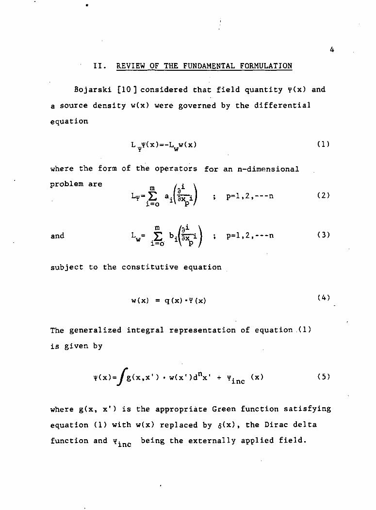
Bojarski [10] considered that field quantity Y(x) and
a source density w(x) were governed by the differential
equation
L y(x)=-L w(x) (1)•f W
where the form of the operators for an n-dimensional
problem are / i \
%-E ailn) 5 P-1.2,— n (2)i=o v P /
and Lw= £ bi(lx ) 5 P-1.2.— n (3)
subject to the constitutive equation
w(x) = q(x)
The generalized integral representation of equation (1)
is given by
w(x')dx' + v. (x) (5)
where g(x, x1) is the appropriate Green function satisfying
equation (1) with w(x) replaced by <s(x), the Dirac delta
function and Hfinc being the externally applied field.
5
Equation (5) is the basic equation which is to be solved by
application of a transform technique.
The Fourier transform of a function f(x) is given as
f(k) = / f(x)ejk*xdx (6)Land the transform pairs formed are noted as f(k) •*•»• f(x).
Thus, by taking the Fourier transform of equations (1), (2),
and (3), the k-space formulation of the problem becomes
L (kmk)=L (k)w(k) (7)T "
£ a.(jk)1 (8)i=o x
mk)-Z Vjk)
where j is the usual imaginary counter-clockwise rotation
operator. The integral equation (5) then becomes
(10)
still subject to the conditions of equation (4). This
approach yields two algebraic equations which may usually
be solved with much less effort than equation (5). With
6
this thought in mind, we now examine the application of
this procedure to the problem of electromagnetic scattering
from a periodic structure.
The electric field E generated from an equivalent mag-
netic source R can be represented by
E(x,y,z)= — VxF(x,y,z) (11)
where F is the associated electric vector potential of the
source and e is the permittivity of the medium [13] . The
relationship between F and K is established with the use of
the position vector r and the free space Green function
A /\
. ' . -j (k-r) =G = - - I (12)
4ir|fl
by -F(r)=/G(r,fI)'K(rl)dr' (13)c=/G(r,fIA
where k and r are the respective unit vectors of the problem.
From this, the magnetic field intensity H can be derived
from Maxwell's equations and is given by
S(x.y.z)— J«e F(x,y,z)+ vy^x.y.z) (14)
where p is the permeability of the medium. For the xy
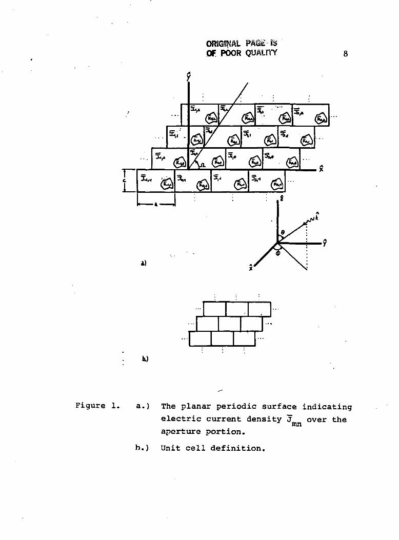
planar set of magnetic currents shown in Figure 1, F =0 is
obtained from equation (13) since z=0 and G is then a
function of x and y only. Allowing the medium to be that
of free space, i.e. e=e oandy=y , and since F =o, equa-
tion (14) is expanded in Cartesian coordinates x and y to
yield for z=0
H (x,y)= -r -s 3 J am
a.3F
2
3.3F,
a,9F,
(15)
where k = 01 :1 e is the propagation constant. The quanti-
ty given by equation (15) is a general representation for
the scattered magnetic field intensity generated from a
planar source of magnetic current in the xy plane.
Consider the planar periodic surface shown in Figure 1
to be the source distribution for che magnetic field of
equation (15). Upon substituting equation (1.3) into equa-
tion (15) and taking the Fourier transform of equation (15)
we obtain
mn
2 2o mn
amn'mn
k 2-K
(16)
B y)'
ORIGINAL PAGE-ISOF POOR QUALfTY 8
Figure 1. a.) The planar periodic surface indicating
electric current density J over themnaperture portion,
h.) Unit cell definition.
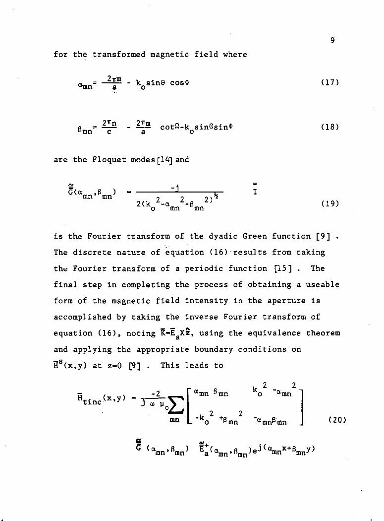
for the transformed magnetic field where
- k sinG cos*a o (17)
a_k sinesin$o (18)
are the Floquet modes [14] and
' CL 8 ^k mn' mn'(19)
is the Fourier transform of the dyadic Green function [9] .
The discrete nature of equation (16) results from taking
the Fourier transform of a periodic function [15] . The
final step in completing the process of obtaining a useable
form of the magnetic field intensity in the aperture is
accomplished by taking the inverse Fourier transform of
equation (16), noting K=E Xz, using the equivalence theorem3.
and applying the appropriate boundary conditions on
Hs(x,y) at z=0 [9] . This leads to
,2 2Htine (x,y) =
-2J
mn
mn amn
(20)
10
where a(a ^mn) "s tne transf°rmed electric field in
the aperture and tinc^x»y^ is the incident tangential mag-
netic field. The inverse of equation (20) is obtained by
extending the operations over the entire unit cell. The ex-
tended operator is necessary to insure the operations in-
dicated by equation (20) are in the domain of the solution.
That is, the boundary conditions of the problem are satis-
fied. This extension is accomplished by including the elec-
tric current density over the conducting portion of the
unit cell. The electric current density is included by in-
troducing the truncation operator and the complement trun-
cation operator defined .as
T(f(f)) = 0 for r on the conductor(21)
T(f(f)) = f(f) for r in the aperture
and
T (f(f)) = 0 for r in the aperture_ (22)
T (f(r)) = f(r) for r on the conductor
This allows equation (20) to be extended over the unit
cell as
am
amn8mn ko2 "amn
112
(23)
with J(x,y) reprsenting the electric current density on the
conductor. Equation (23) is a form which can readily lend
itself to solution by iterative techniques.
12III. MATHEMATICAL FORMULATION OF ITERATIVE EQUATIONS
CONTRACTIONS AND FIXED-POINT THEORY
The use of iterative equations to solve mathematical
problems has been around for many centuries dating back to
B.C. 600 when this technique was used to solve problems
such as determining the square root of three. Beginning
with this early exploration of iterative techniques came
the plights of correct problem formulation and convergence
of the solution. Later methods, such as Newton's method of
solution, alleviated such problems but often forced other
constraints on the problem. One such constraint is that
the initial solution estimate needs to be in a region
reasonably close to the desired solution. Tsao and Mittra
[9] used this spirit of a priori knowledge in the form of
a variational correction to remain near the solution point
in their problem formulation. However, as will be demon-
strated later, the cases presented in their work did not re-
quire such a correction and, indeed, they even noted where
the iteration method failed even using such a correction.
The idea of using the iterative scheme to solve gener-
al scattering problems leads one to seek a way of determin-
ing the criteria for convergence and a way of generating a
convergent iterative formulation. Fixed-point theory and
contractor theory [16, 17] are applied to formulate a con-
13
vergent iterative solution to the scattered fields derived
in Chapter II.
The general idea of fixed-point theory revolves around
finding the solution to an equation such as
f(x) = y = x 2 - 6 x + 5 = (x-5) (x-1) = 0 (24)
This is accomplished by forming an iteration function as
xn+1 = g<V (25)
and finding the intersection y=g(x ) and y=x which yields
the fixed-point and solution to equation (24). This is
accomplished by starting with an initial guess x , substi-
tuting into equation (25) to generate x,, and continuing
this process until x +1=x +e where e is the allowed error.
At this time x=x , is the approximate solution to equation
(25). The conditions for a convergent solution are in
general:
a.) on a closed interval I, g(x) maps I into itself
b.) g(x) is continuous on I
and c.) g(x) is differentiable on I and de(x) < 1
Thus the following theorem may be stated
Theorem 1. Let g(x) satisfy conditions a.), b.), and
c.). Then g(x) has exactly one fixed
point x* in I and starting with any XQ in
I, the sequence x , x, , ... , x generated
by equation (25) converges to x*.
14
The process outlined by the above theorem is illustrated in
Figure 2. The fixed-point x* is often said to be a point
of attraction for g(x). xn+i is also said to contract to
x*.
To illustrate the use of this theory, one root of equa-
tion (24) will be determined. Let
(26)
and find
d g(x) = -* (27)
then, the interval I is defined as xtl and IcC-3,3]. Note
that the known root x=l is in this interval and
-T— g(x) =1/3. We then expect that the iteration function
will converge to the fixed-point x*=l which is the correct
solution. The iterative process is contained in Table 1.
The question then arises, what happens when the sequence
will not converge?
To generate an iterative equation that will convege we
must meet the conditions listed in Theorem 1 above. As an
example, let us examine the roots of
f(x) = x2 - x - 6 = (x+2) (x-3) (28)
15
:\a N
s01
s
8
S•«l
S S S s
X!
bO
Co
ctf
O"
0•*->
c0)bO
<»coo
o<DQ,
X!
CM
0)
3bO•H
16
f(x) = x2 - 6x +5 = 0
x2 + 5g(x) **
X0xl
x2
X3
X4 -
X5
* £
6
g(x)
2.0
1.5
1.208
1.077
1.026
1.009
1.003
xn-l
x*=x 1.000n
Table 1. Example of a convergent iterative equation
17which can be seen to be -2 and 3. By forming the iterative
equation
= xn+l=xn (29)
and noting
(30)
we see that the iterative equation will not converge. How-
ever, by properly forming a new iterative equation G(x)
that has G(x) x=-2<1 or G(x) x= , the roots
may be obtained. Although manipulation of equation (29)
could yield a suitable G(x) [12] we seek a G(x) that can
be formed by a method known as relaxation. The relaxation
process generally uses a portion of the n iteration alongt~Vi
with a portion of the iterated n (i.e. n-t-1) iteration to
"relax" the process. The form of the relaxed iterative
equation is
G(x (l-R)g(xn) (31)
where R is called the relaxation constant. The condition
=0x=x
(32)
nmay be used to determine an optimum R such that convergence
18
of G(x) is assured. Performing the operation of equation
(32) on equation (31) yields
4- G(x)dx = R+U-R) 4- S<x)dxx=x
= 0 (33)
x=xn n
and solving for the linear correction R
where g'(x)= -7— g(xj. This process of finding the optimum
nR is called the contraction corrector (a name to be ex-
plained later in this section) and is used to iteratively
solve for the root x=3. This is illustrated in Table 2.
Equivalence between the contraction corrector and Newton's
method can be shown and is illustrated in Appendix C.
Note that g(x ) would not converge by itself and thus G(x)
is necessary for a correct solution to be obtained. As a
further note on the iterative process, the conditions that
g(x) maps I into itself is not trivial. For instance, note
that
f(x) = x2 + 2 = 0 (35)
will not yield a solution from an interative process unless
x is allowed to be complex and g(x) or G(x) maps into the
complex plane. The iterative equation G(x) may even re-
quire a complex relaxation or complex contraction correc-
tion constant and precautions governing complex algebra
19
- xn+l = xn - 6
x_.,= G(x ) =n = Rxn=
(1-R)
2 xn
n
0
1
2
3
4
Xn
1.0
7.0
4.24
3.23
3.01
Rn
2.0
1.07
1.13
1.18
1.2
n
1
2
3
4
5
6
2x
g(xn)
-5.0
43.0
11.98
4.43
3.06
^3.0001
3.0006
3 . 0036
3.0216
3.130
3.798
G(xn)
7.0
4.24
3.23
3.01
3.0
g(xn)
3.0006
3.0036
3.0216
3.130
3.798
8.424
Table 2. Example of a non-convergent iterative equation
with convergence achieved by applying the con-
traction correction method.
20
and operations must be observed. In particular, the ana-
lytic nature of f(x), g(x), and G(x) in the interval I
should meet the requirements of Theorem 1. An illustration
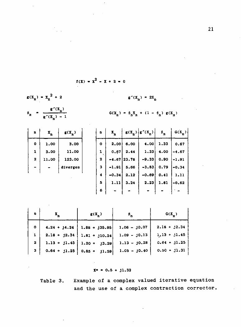
of the nature of these problems is given in Table 3. In
two cases, a real x never maps x into the complex plane
and, as such, never yields a solution. Even applying the
contraction corrector method with a real x does not give a
solution. Only the one case using a complex x and the con-
traction corrector method converges. This follows from the
conditions of Theorem 1. Since problems have been observed
in the simple problems above, a proper choice of action is
to pursue the corrective method in a more general sense.
Stakgold Cl8l has formed a very sound collection of
theorems and definitions on the idea of metric spaces and
their transformations, and the following material is con-
densed from his book with the advice that the reader con-
sult his work for proofs and greater detail.
Definition 1. A transformation L of a metric space
x into itself is Lipschitz continuous
if there exists a p, independent of u
and v, such that
d(Lu,Lv)_< pd(u,v) for all u,v£x
where d(C,£) is a proper metric in x. When the definition
above holds for some fixed \p( <1 , the operation of L is
called a contraction on X.
f(X) - X - X + 2
21
g'(Xn) 2X_
g'(XQ)G<Xn> - 6 X + (1 - B ) g C X i
ff*(X ) — 1 n n n n n
n
0
1
2
-
Xn
1.00
3.00
11.00
-
g(xn>
3.00
11.00
123.00
diverges
n
0
1
2
3
xn
4.24 ••• J4.24
2.18 + J2.34
1.13 + jl.45
0.64 •«• jl.25
n
0
1
2
3
4
5
6
Xn
2.00
0.67
-4.67
-1.91
-0.34
1.11
—
g(xn>
1.88 + J35.95
1.81 •»• J10.24
1.20 * J3.29
0.85 •*• jl.59
g(xn)
6.00
2.44
23.78
5.66
2.12
3.24
—
g'cxn>
4.00
1.33
-9.33
-3.83
-0.69
2.23
—
Bn
1.06 - jO.07
1.09 - jO.13
1.13 - J0.28
1.05 - JO. 40
6n
1.33
4.00
0.90
0.79
0.41
1.81
—
G(Xn)
0.67
-4.67
-1.91
-0.34
1.11
-0.62
-
G(XD)
2.18 •»• J2.34
1.13 + jl.45
0.64 t- jl.25
O.bO * jl.31
X* - 0.5 -f jl.32
Table 3. Example of a complex valued iterative equation
and the use of a complex contraction corrector.
22
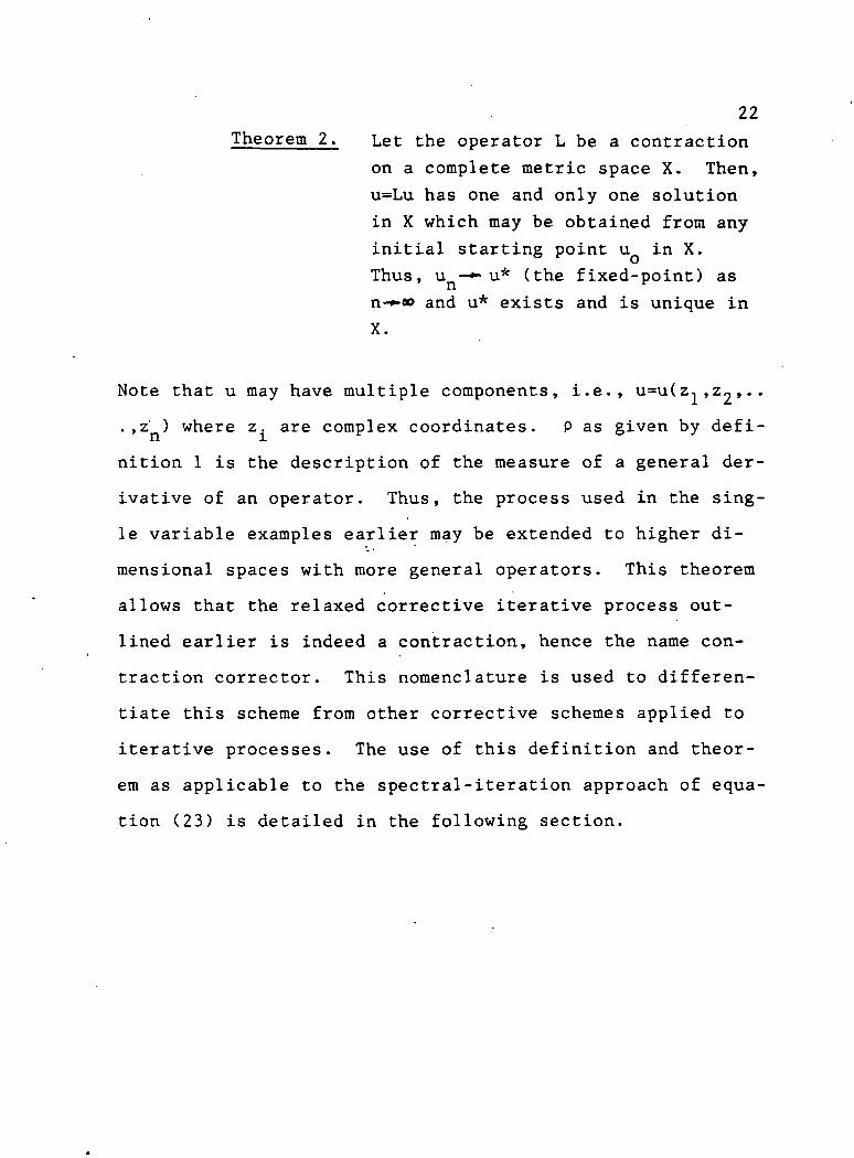
Theorem 2. Let the operator L be a contraction
on a complete metric space X. Then,
u=Lu has one and only one solution
in X which may be obtained from any
initial starting point u in X.
Thus, u -*• u* (the fixed-point) as
n-*-» and u* exists and is unique in
X.
Note that u may have multiple components, i.e., u=u(z,,Z2,..
. ,z ) where z. are complex coordinates. P as given by defi-
nition 1 is the description of the measure of a general der-
ivative of an operator. Thus, the process used in the sing-
le variable examples earlier may be extended to higher di-
mensional spaces with more general operators. This theorem
allows that the relaxed corrective iterative process out-
lined earlier is indeed a contraction, hence the name con-
traction corrector. This nomenclature is used to differen-
tiate this scheme from other corrective schemes applied to
iterative processes. The use of this definition and theor-
em as applicable to the spectral-iteration approach of equa-
tion (23) is detailed in the following section.
23
IV. THE PERIODIC STRUCTURE; A
CANONICAL CASE AND THE REGIONS OF SOLVABILITY
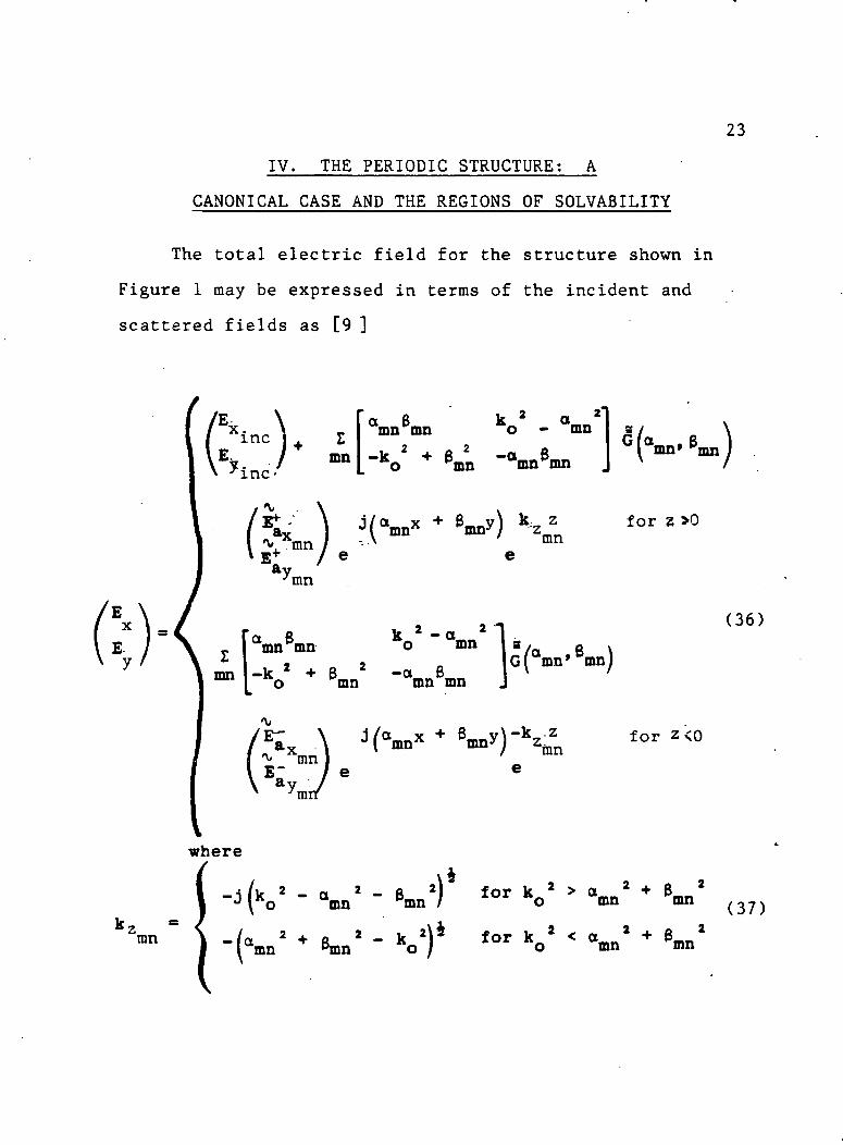
The total electric field for the structure shown in
Figure 1 may be expressed in terms of the incident and
scattered fields as [9 ]
E,Zmn
amn mn o - mn
~°mn mn
v mn
ran
x
ZmnIamn mn B -a Bmn mn
2 1mn Is,
K1mn J
(36)
°mn' mn
mn-k -z
zmne
for z<0
a
wherex
mn
~ mn '°r ko2 » °mn2 + Bmn2
1 tor k.1 < a* + * z(37)
24= =
and E and E represent the transformed electric fielda a r
and are respectively the reflection and transmission coef-
ficients of the Floquet modes. Deriving H from equation
(36) and by enforcing the boundary conditions on the tan-i
gential magnetic fields across the cell at z=0, equation .
(23) is generated again. This exercise is presented to
complete the field description and to illustrate the rela-
tionship between the aperture fields and the reflection and
transmission coefficients as the coefficients will be of
interest later in the section. Equation (23) is the begin-
ning point to cast the problem in an iterative form.
The summation in equation (23) represents a discrete
Fourier series (DPS) for an infinite duration (i.e., peri-
odic) sequence [19] . This representation allows for direct
transformation between the (x,y,z) domain and the (k ,k >k )x y z
domain. Since the functions are represented by sequences
with complex exponentials having a periodicity of 2ir/m and
2ir/n, one period of the aperture distributions, that is one
cell of the structure, can be used to completely specify the
transform. The use of one period to represent a periodic
function in this manner is known as the discrete Fourier
transform (DFT). It is important to note that the trans-
formation mentioned above is exact and this infers that no
aliasing will occur when the DFT is performed. Aliasing
can occur when a non-periodic function is truncated and
25
and transformed with a DFT. Since information about the
original function is lost in the truncation, performing the
inverse transform can never return the original function.
However, when using exactly one period of the periodic func-
tion, the original function can be reconstructed when the
DFT and inverse DFT are performed. The most common form of
DFT algorithm is the fast Fourier transform (FFT) in which
special properties of the DFT are exploited to decrease the
computation time of the transform. Throughout this section,
the DFT and its inverse are represented by F and F re-
spectively. Implicit functional dependence is also used to
present a "cleaner" form of "the equations.
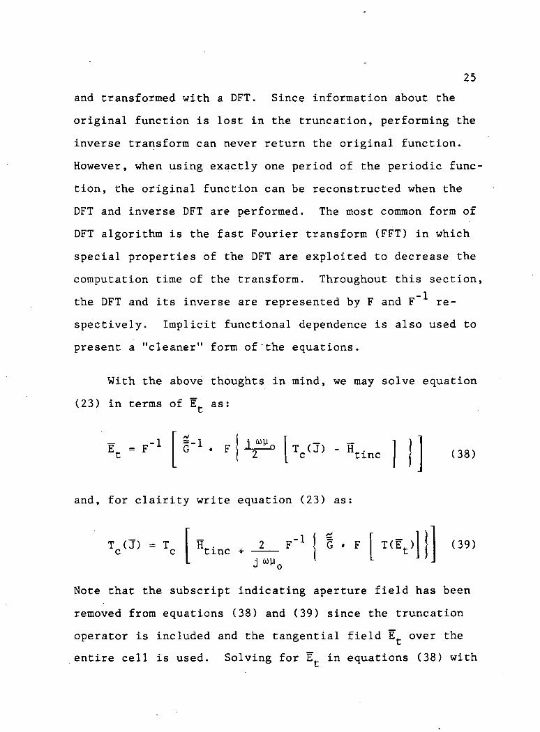
With the above thoughts in mind, we may solve equation
(23) in terms of E~ as:
,-1 G"1 • F VJ) - Htinc (38)
and, for clairity write equation (23) as:
T (J) = Tc ctitine +
,-1 8 T(Et) (39)
Note that the subscript indicating aperture field has been
removed from equations (38) and (39) since the truncation
operator is included and the tangential field E over the
entire cell is used. Solving for E in equations (38) with
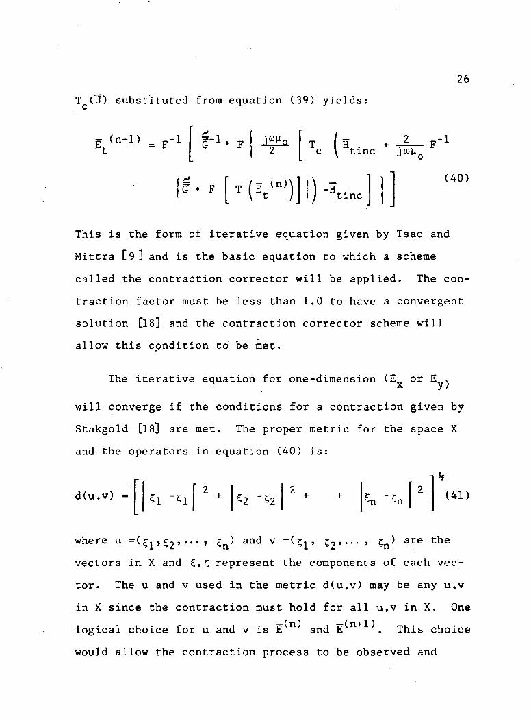
26
T (J) substituted from equation (39) yields
«• (n+1)Et
p= F
-1
*.F [T(lt<»>)] "Htinc
(40)
This is the form of iterative equation given by Tsao and
Mittra [9] and is the basic equation to which a scheme
called the contraction corrector will be applied. The con
traction factor must be less than 1.0 to have a convergent
solution [18] and the contraction corrector scheme will
allow this condition to" be met.
The iterative equation for one-dimension (E or E x y}
will converge if the conditions for a contraction given by
Stakgold [l&] are met. The proper metric for the space X
and the operators in equation (40) is:
d(u,v) = (41)
where u =( > g2, ... , £n> and v =(?1» ?2"" ' are the
vectors in X and Ct z, represent the components of each vec-
tor. The u and v used in the metric d(u,v) may be any u,v
in X since the contraction must hold for all u,v in X. One
This choice
would allow the contraction process to be observed and
logical choice for u and v is E and E
27
would give the relative error between each iteration. This
also allows the regions of convergence to be determined.
That is, for decreasing error, the solution is converging
and for increasing error diverging. Since we are interest-
ed in the contraction to a fixed-point, a wiser choice for
u and v is E and ^E~ + e) where e is some small complex
number. Thus, at each component of E~ we essentially
have the ability to determine the general derivative of the
operator at each element. The contraction corrector is a
vector R with one element for each component of E
The form of R is exactly that of equation (31) for a one-
variable problem extended to an N component one-dimensional
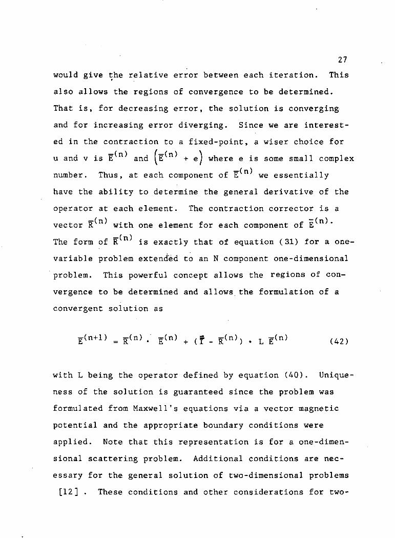
problem. This powerful concept allows the regions of con-
vergence to be determined and allows the formulation of a
convergent solution as
R(n) •' E(n) + (? - R(n)) • L E(n) (42)
with L being the operator defined by equation (40). Unique-
ness of the solution is guaranteed since the problem was
formulated from Maxwell's equations via a vector magnetic
potential and the appropriate boundary conditions were
applied. Note that this representation is for a one-dimen-
sional scattering problem. Additional conditions are nec-
essary for the general solution of two-dimensional problems
[12] . These conditions and other considerations for two-
28
dimensional problems are discussed in Section VI.
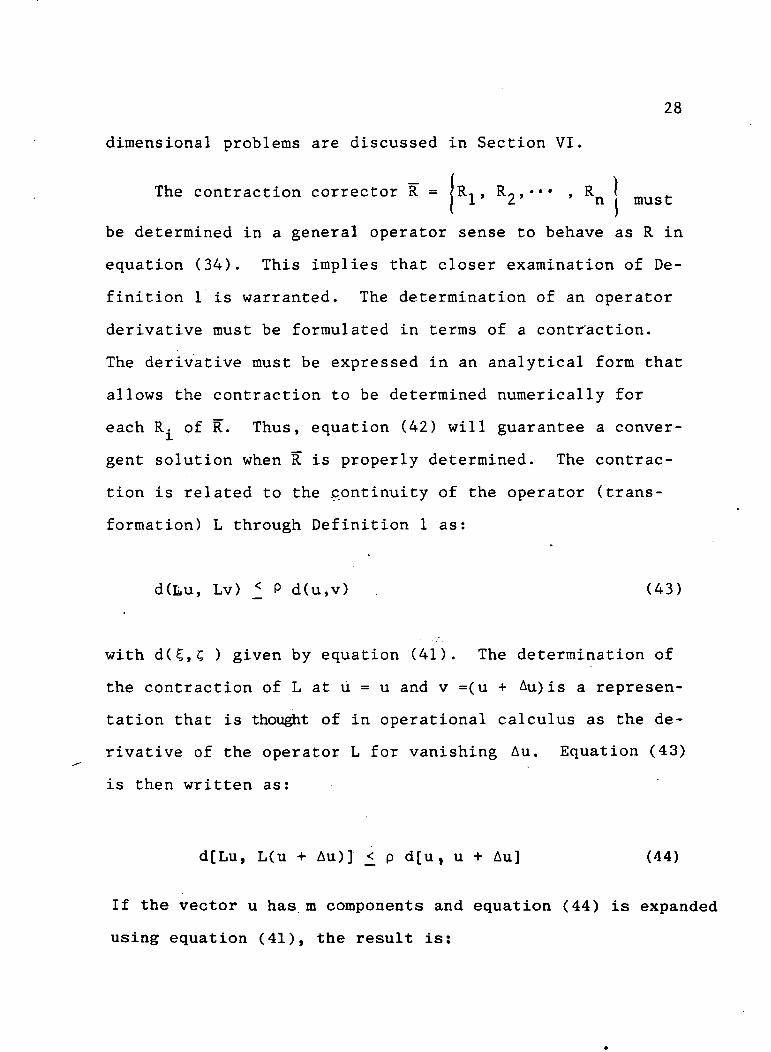
The contraction corrector R = < R i » RO'"' ' Rn must
be determined in a general operator sense to behave as R in
equation (34). This implies that closer examination of De-
finition 1 is warranted. The determination of an operator
derivative must be formulated in terms of a contr'action.
The derivative must be expressed in an analytical form that
allows the contraction to be determined numerically for
each R. of R. Thus, equation (42) will guarantee a conver-
gent solution when R is properly determined. The contrac-
tion is related to the .continuity of the operator (trans-
formation) L through Definition 1 as:
d(Lu, Lv) < P d(u,v) . (43)
with d(C,C ) given by equation (41). The determination of
the contraction of L at u = u and v =(u + Au)is a represen-
tation that is thought of in operational calculus as the de-
rivative of the operator L for vanishing Au. Equation (43)
is then written as:
d[Lu, L(u + Au)] <_ p d[u, u + Au] (44)
If the vector u has m components and equation (44) is expanded
using equation (41), the result is:
29
,. +Au)-Lu, + L(u_+Au) - Lu01 i\ \ 4 A
< P
Ku1+Au)-u1 •J
•(45)
Eliminating terms in the denominator of equation (45) yields
+ . L(u +Au)-Lu_ f< P (46)
m l A u l
Now, since m>l, a stronger condition is written
I2 + |L(u2+Au)-Lu2|2 +.-.+I
P (47)
Consider the following: given
12 ; I 12 Ai[!• "* a2 *—* am (48)
30
Is the inequality true? Squaring both sides yields:
m(49)
m a. m
and the inequality is seen to be valid for non-zero a..
Equation (47) is then written as:
L(u,+Au)-Lu, Au)-Lu L(um+Am)-Lu
Au
< p (50)
and then may obviously be further reduced for each component
t0: L(ui+Au)-Lu11 Pi (51)
Au
noting that -f^P- < P»
From equation (51) it is
be defined and the final form of equation (51) becomes:
From equation (51) it is seen that a complex-valued p mayci
L(u.+Au )-Lu.
Au= P
Ci(52)
This form is the measure of the derivative of the
operator L at each component and may be used to solve for
the contraction corrector R. at each component u- e u.
31
Even though a powerful tool has been developed to
allow the computation of a convergent one-dimensional solu-
tion to electromagnetic scattering, the background problems
surrounding the contraction corrector scheme should be ex-
amined. This.background material is of interest since the
breakdown of prior methods and the reasons for non-conver-
gent solutions gives insight into what particulars of the
scattering problem cause the difficulties. In particular,
known geometrical problem areas are: conductor width, cell
size, aperture size, and the angle of incidence and polari-
zation of the impinging plane wave. The understanding of
the difficulties arising for certain values of those para-
meters can provide vital insight when attempting to extend
the solution to two-dimensinal configurations, especially
when mesh structures are involved. The reference point for
this background investigation is the work of Tsao and Mittra
[9] . A complete iterative flow is detailed in Appendix B.
Consider the case of the free-standing strips shown in
Figure 3. This planar configuration of thin, perfect con-
ductors was the prime example used in the work of Tsao and
Mittra [9] . The case of a cell width of 1.4X , aperture
width of 0.6x , and incidence angle 0=0* was of particular
interest. Although the iteration equation (40), would per-
form adequately, Tsao and Mittra decided to apply a correc-
tion step to the iterative process. The idea of being
"near" the solution in numerical methods (i.e., Newton's
32
ConductingStrips
>H-ncfinc
$5r$• ifi,, v'.-y-»fjff*Kl:- JivjE-S-M
4
X
Figure 3.Free-standing conducting strips with Floquetcell width a, aperture size b and conductivity
o.
33
Method) to either insure or speed convergence is commom
place. The correction step was chosen to be a form of the
Method of Moments [28] .
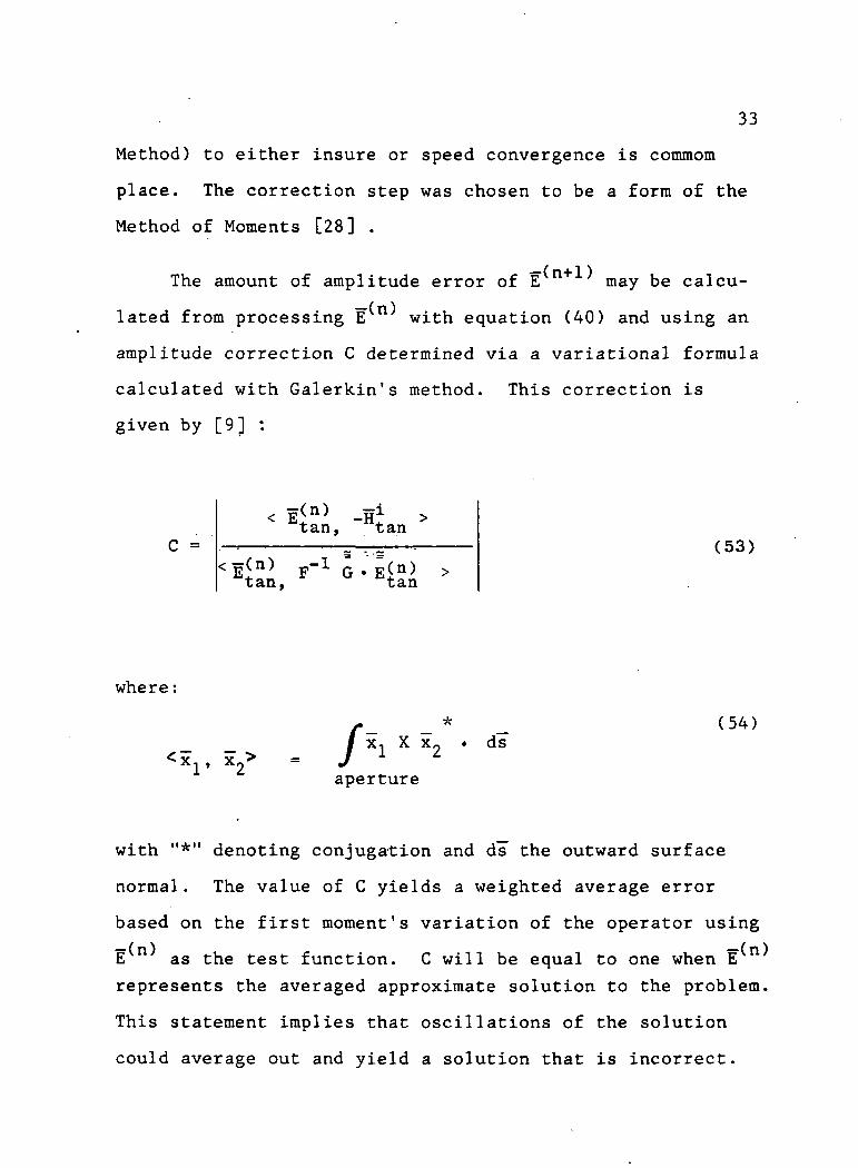
The amount of amplitude error of IT may be calcu-
lated from processing E with equation (40) and using an
amplitude correction C determined via a variational formula
calculated with Galerkin's method. This correction is
given by [9] :
C =tan, tan
tan
(53)
where:
(54)ds
aperture
with "*" denoting conjugation and ds the outward surface
normal. The value of C yields a weighted average error
based on the first moment's variation of the operator using
E n as the test function. C will be equal to one when E
represents the averaged approximate solution to the problem.
This statement implies that oscillations of the solution
could average out and yield a solution that is incorrect.
34
Numerical difficulties could then arise if a problem gener-
ated such a solution from the iterative process. Great
care is then warranted with this type of numerical method
as is true with any numerical scheme. Additionally, as pre-
viously noted for iterative processes, just being near the
correct solution in amplitude does not guarantee a conver-
gent process.
The geometry given in Figure 3 for a=1.4X, b=0.6X, 0=0°
and H-wave (E.. parallel to strip edges) incidence is a11 no
problem that converges by equation (40) without the aid of
the variational correction of equation (53). What then is
the useful purpose of the correction C? The most useful
purpose of C is to speed convergence since an iterative
equation which is a contraction will converge from any ini-
tial estimate and will diverge if not a contraction. Anoth-
er useful (but applied with caution) purpose is the indica-
tion of accuracy of the iterated solution. The problem
above is taken from Tsao and Mittra [9] . The convergence
of the problem is shown in Figure 4. Figure 5 illustrates
the convergence of E of the problem using equation (40)
corrected by C of equation (53). The iterations of both
Figure 4 and Figure 5 are quite similar; however, the E n
shown in Figure 5 are converging more rapidly then the E
in Figure 4 by one iteration. This is a very small difference
in convergence rates and indicates that the methods behave
similarly.
35
bec•H-P 0,O -H3 t-(•a -Pc wOO
0)
0)a
BX
CD O
CO•
OIIft
IIaS
O«H
•H<H
-pJH0)
d
CO•H-P
o*0)
O -HCD
oC <D0) (0
h O<D> oc oO IIo o
•<*a)
bC•Hfe
36
37
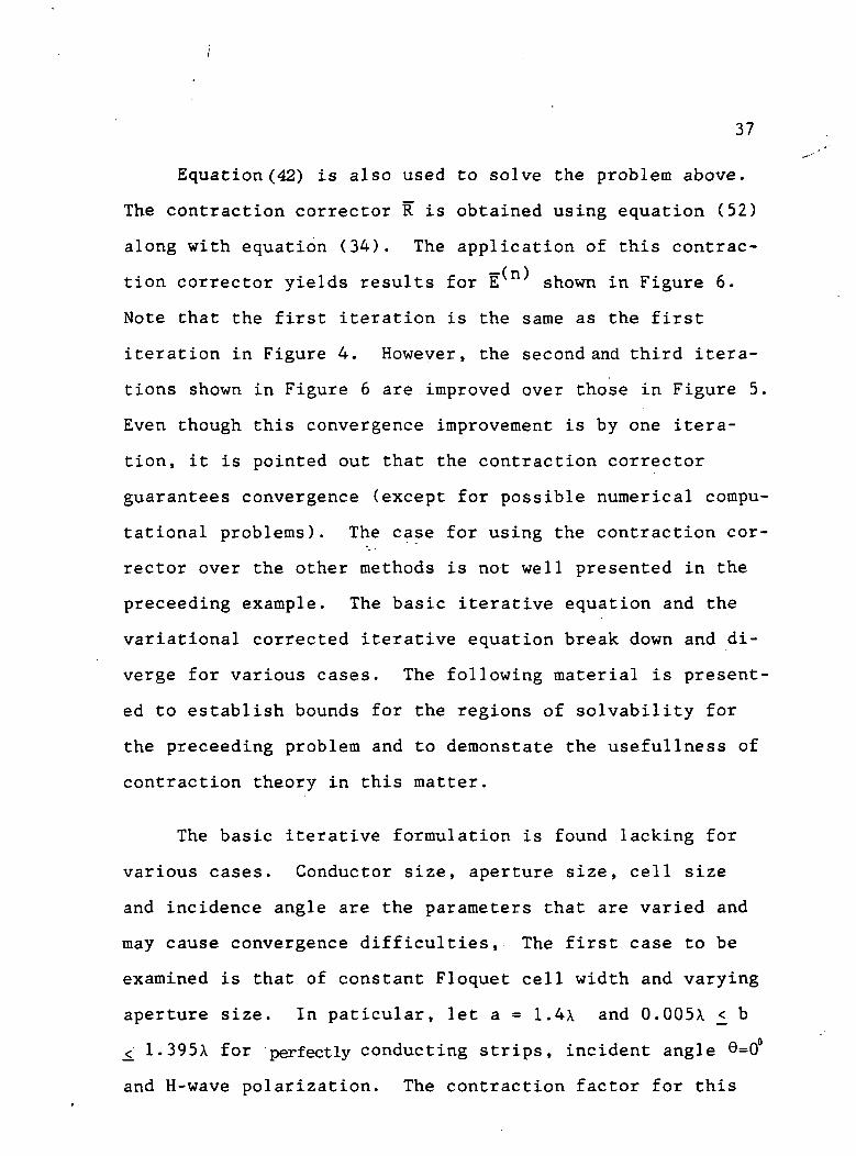
Equation (42) is also used to solve the problem above.
The contraction corrector R is obtained using equation (52)
along with equation (34). The application of this contrac-
tion corrector yields results for E shown in Figure 6.
Note that the first iteration is the same as the first
iteration in Figure 4. However, the second and third itera-
tions shown in Figure 6 are improved over those in Figure 5.
Even though this convergence improvement is by one itera-
tion, it is pointed out that the contraction corrector
guarantees convergence (except for possible numerical compu-
tational problems). The case for using the contraction cor-
rector over the other methods is not well presented in the
preceeding example. The basic iterative equation and the
variational corrected iterative equation break down and di-
verge for various cases. The following material is present-
ed to establish bounds for the regions of solvability for
the preceeding problem and to demonstate the usefullness of
contraction theory in this matter.
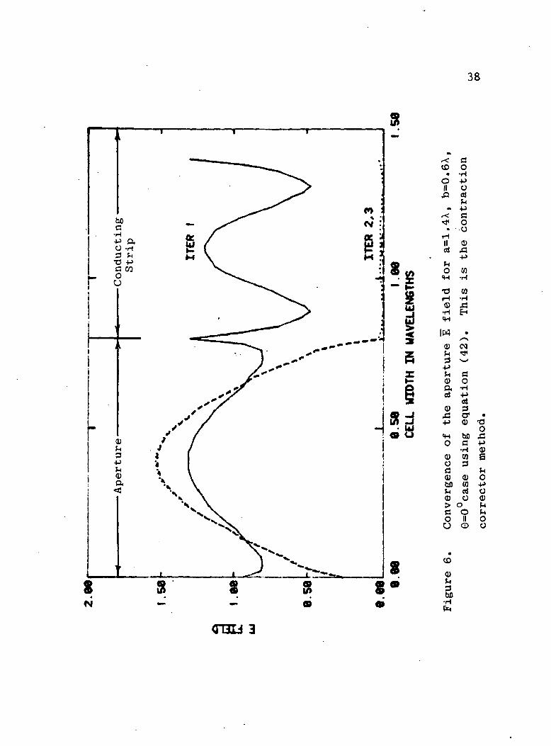
The basic iterative formulation is found lacking for
various cases. Conductor size, aperture size, cell size
and incidence angle are the parameters that are varied and
may cause convergence difficulties, The first case to be
examined is that of constant Floquet cell width and varying
aperture size. In paticular, let a = 1.4X and 0.005A <_ b
_< 1.395X for perfectly conducting strips, incident angle 9=0
and H-wave polarization. The contraction factor for this
38
r< C
CO O• -H
O -PII Of^ QJ
• -P.-< C^fl O• o
II 0-p
CO•H
CO
o<H
73
0•H<H
IW
0fn
0 OD, -Hcd -P
OJ
0 3X! 0« ••P 0 T3
O•H bD SiO G -P
•H 00 CO g
(HO
IM
Ofi0 0M M -PJH OS O0 O 0> O F-iC O MO II Ou o o
CO
0VlbO•H
CT3LJ 3
39
I
8
sa
0)oc
oc
-PTJ
a)o
o<H
o•PocS
«H
Co
ort-Pcoo
t^0)
3to
oII
•3Cat
CO
«51S1•H
rtrHOD,
0)
rf
oIIo
bCCai
POOR QUALrTY
40
»
oc0•o•Hoc
o•
o«Ho
•M•a
-P01
oJ
oOII
Co
03tsl•H
OQ.
c
_ *ȣ 3j "i
,£
•
0
O
0
£c0•H•p0
?H
^Jco0
00
0)
Oj
1K
-P•H?
0
oII0
Q)r-lhflc0*
<*> M
41
case is graphed in Figure 7. Recall that the solution will
diverge for a contraction factor greater than one. These
non-convergent regions are where the contraction corrector
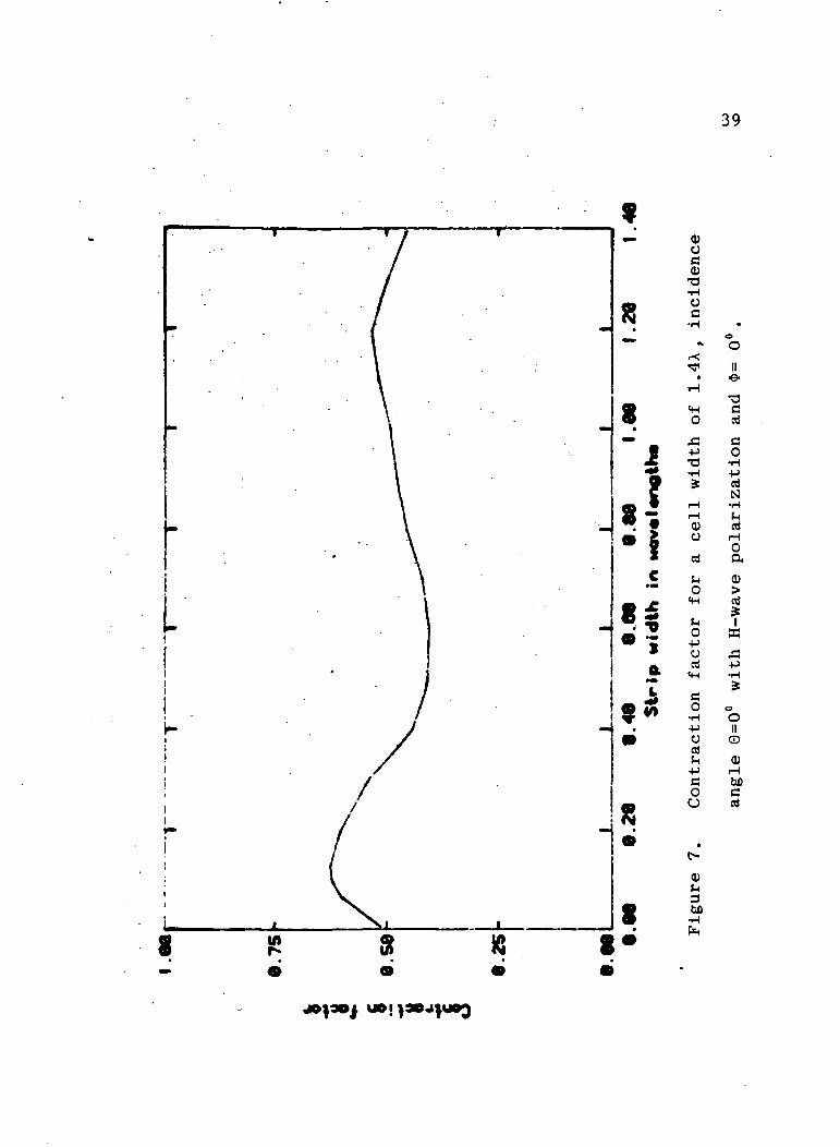
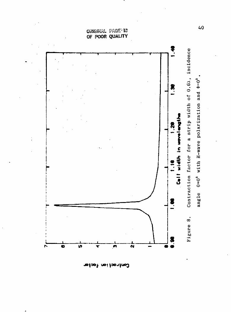
must be applied to insure covnergence. Next, the cell size
is varied as 0.9x <. a <_ 1.4x for constant conductor size,
i.e., (a-b) = constant, and 0= 0° with H-wave polarization.
Figure 8 shows the contraction factor for a conductor size-
0.8X . This last example contained a conducting strip that
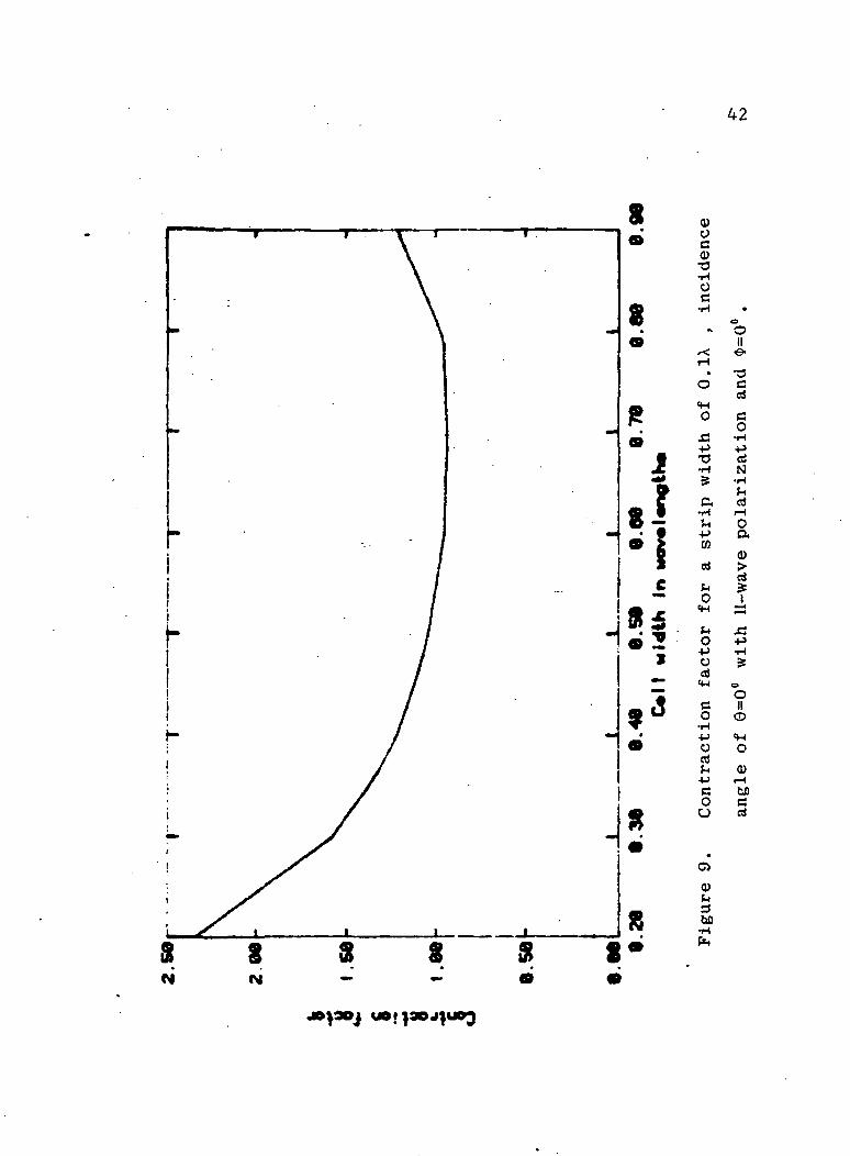
was a large portion of a wavelength. The case of a conduct-
or size 0.1X and cell width 0.2 A _< a _^ 0.9 A for H-wave po-
larization and 0= 0° is presented in Figure 9. This example
represents a small strip and the contraction factor associ-
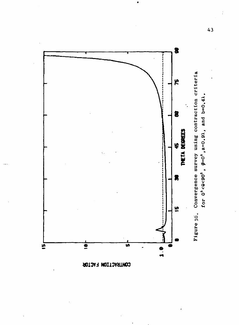
ated with its geometry. The last case to be examined is co-
cerned with the angle of incidence of the impringing plane
wave. A cell width a = 0.9X , conductor width b = 0.4 A
and aperture width 0.5X is chosen for the convergence sur-
vey illustrated in Figure 10. Note that the contraction
factor bumps above 1.0 around 0 = 8 ° and diverges from 1.0
for 0>60°. This indicates that the basic iterative scheme
will have problems with convergence around 0 = 8 ° and wills
not converge for 0>60°. The above examples offer several
cases that point out problem areas in constructing a conver-
gent iterative solution.
The contraction corrector may be applied to construct
a convergent solution when the basic iterative scheme
0)oc<p•o•Hoc•H
<HO
AP•O
•PM
erf
J*O
o•Poerf
CO
oerf
CO
O
-3bC
•e-
Cerf
CO•HPerfN
erf
Oa
erf
1
OIIO
(UtHt£Ccrf
8N
8N
43
8
8
IHCD
c <*O ••H O•p IIO X)cdfn T3•P CC rtOO
.<bO 0)C ••H OCO II9 01
A
>> O
0) O> IIM ©.
COO
0) oO C5C VCU CDW V^ o<u oC (-.o oO «H
0)
hO•Hfa
in IA
44
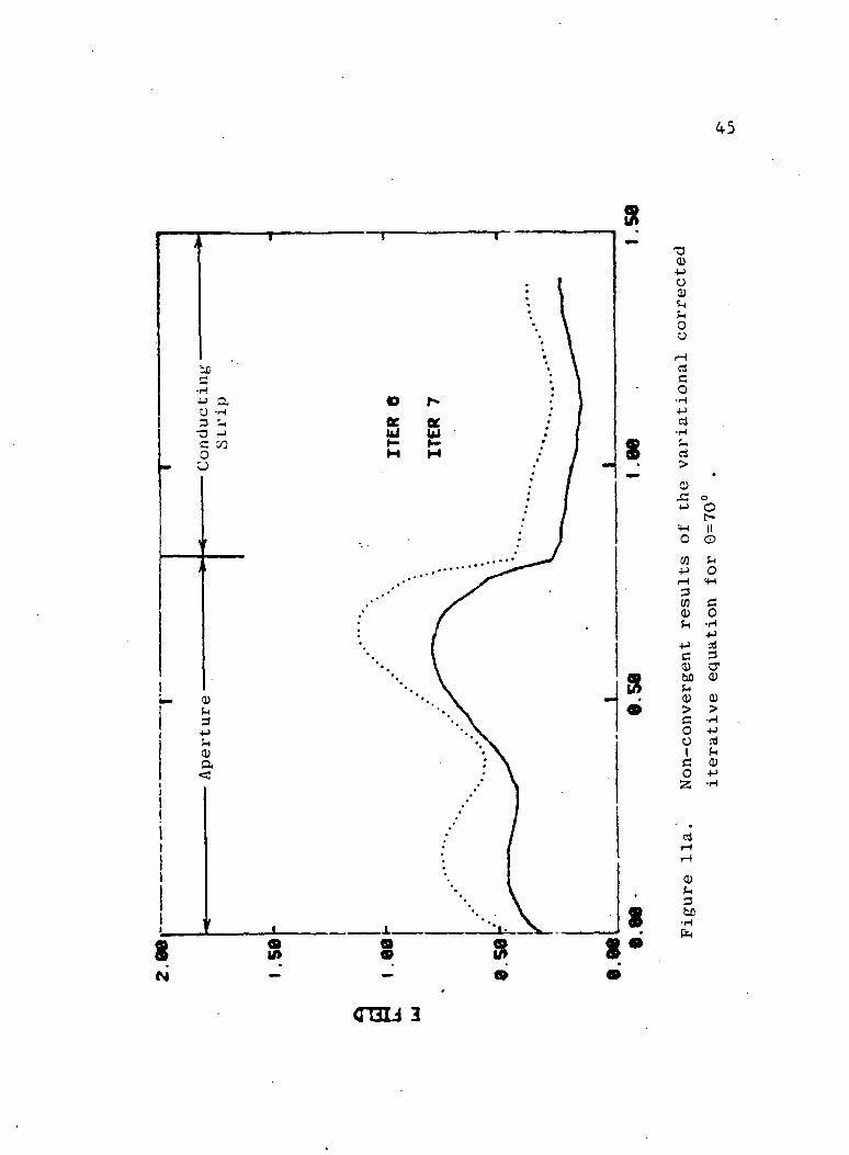
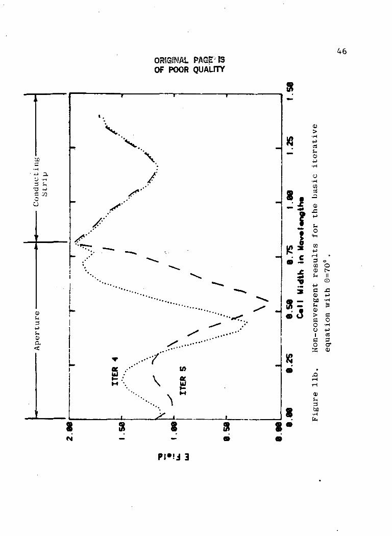
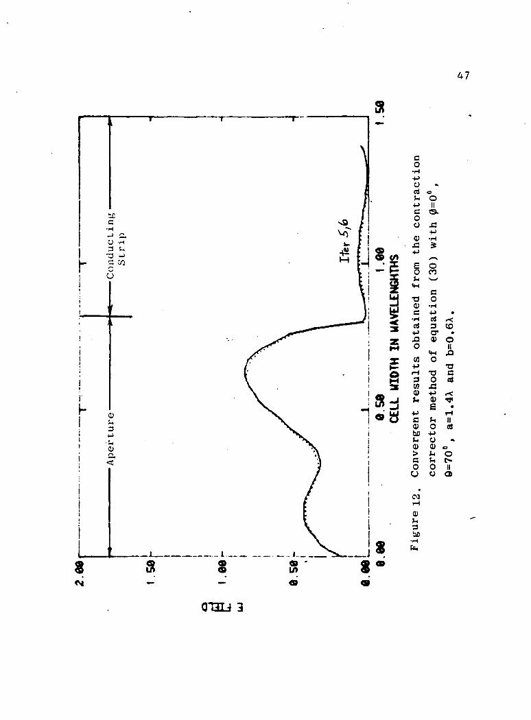
breaks down. Consider the case of Figure 3 with a = 1.4 A,
b = 0.6X and 0= 70° . At this incidence angle, the itera-
tion equation (40) and variational correction of Tsao and
Mittra [9] break down and do not converge. Figure 11 illu-
strates that after six and seve'n iterations respectively,
neither method converges. However, Figure 12 reveals that
the contraction corrector method converges after six itera-
tions and has a small error over the conductor. Herein
lies the reason the contraction corrector method is pre-
ferred. Even when the basic method and variational cor-
rection schemes fail to converge, the contraction cor-
rector method assures that solution can be reached and does
so with reasonable ease.
The foregoing examples have demonstrated the ability
of the contraction criteria to be applied to one-dimensional
scattering problems to determine the regions of solva-
bility. Additionally, the contraction corrector scheme has
been utilized to achieve convergence when the basic itera-
tive schemes failed. The examples presented give indica-
tions that the contraction corrector can be successfully
applied to planar wire surfaces.
0)•PoOJ
oo
aco
• H•Prt
d
O
P ot>
"o oOT fiP Or-l VI
CoCO0)
-pc
CooIc
trf
0)
0>•HPd!H0)
3bfl
M
<TI3Li3
OR5QSNAL PAGE ISOF POOR QUALITY
i
'-,X
•H• JJ 0.
CJ -H3 ^O -iJ
5 "°
O
1
,
i
r i 1
* .
V'V\
/•'/?
^. •jf!
S''//• *
/p'/>fr^-
" .•' "**" ^^ —«^
- ^ ^1 * ^^^^^
'••. «»^
»3•Pf-i0>CX,
I
* , m ^^%
* * * ' » . ^*^
" * * * • * ^^
" "-... ..^ ^ -0-* »*
*^^f • *^r^ • • •
• •
•^••"""f • *
*" « .-••' u> "£ / V *M •. \ UJ
'•• \ M
"••.. )
> 1 I
-
o
iu -*-1. rf
•H
o>r^en
B ^
•J «
1:"S o5 'H
in a a?• c d *
9 .Z 3 oW O
X rti t**; ii^ H II
!S ^ °«5 c ^0) -P
. ^ 0) "*-Xs s §O -HO -P
£5 3o cr
«•
T-t
0)
3
8 tor<
8 a 8 a 8*
PI'U 3
47
I-
txc
O -H3 U•a *->c co
5
0)M
3+J
•s-.ooi
<T
<M
co•H
Vt1 ^+»
c00
0)S3•M
EO«_,W
<H
T3/ItW
C•Hrf
-»->J3O
CO•»-»rH30}0)h•pc0)tt>0>>coo
•
CMr4
0)t .H3U)
O
o.£-(->•rts^>on
o,_jf^-Mrt3O1
0)
C^j*r^o
T3OA•M0E»HO
4->00
fc4
Oo
•f<CO•
oIIrtnU
•acA
»<•
T-l
II
ol
«
0
0C-.IIa
OT3U 3
48
V. THE PROBLEM OF AN INFINITE GRATING
OF THIN WIRES
The structure shown in Figure 13 has been studied over the
years by various techniques to determine the reflection co-
efficient from the grid [1 , 2, 20 ]. The reflection coeffi-
cient may be obtained from the transform of the aperture E
field in the form of the Floquet modes. For the case of
cell widths less than ^/2, this coefficient is obtained
from the n = m = 0 element of the E~ variable for the• mn
case of plane wave incidence as [9]
~(n) -(n) -..F = E- = E+ - E . (55)
The first atempt to solve the problem with a X/'4 cell and
A/600 radius wire was performed with the variational correc-
tion iterative process using E n as a test function in the
variational scheme. This method fails to converge for vari-
ous sampling rates and various numbers of Floquet modes,
and a more suitable test function is sought [21] . The
Dirac delta function is chosen as the test function and
gives acceptable results for small angles of incidence.
The delta function samples the response and allows point
matching to be utilized to improve the variational correc-
tion factor. The convergence properties achieved with these
two test functions are shown in Figure 14. Since the iter-
ation method should be convergent for all incidence angles,
C-COJL
50
CO
co3•H
•a
0)
CO
en
co
0).c
co
x^ tp^
-uT3 OC C
Si
cti C
. IW
•PCO0)
.c .c o•P -M 0) II
o A A«H JQ -PO T3
bfl CO Cco c a at0) -H•H CO C *<•M 3 o m<D D -M •a E o oo v e n!-> J3 3 c3O, O «M
to «0) doO C -*-> OC O (H ||a) -H a> <iMl -P TJ IIti O O>Q) (U O
C )H ^ -PO O -H -HO O Q ^
0)h300
oo
51
the development of a different form of correction is a
logical path to follow.
The iterative process of equation (40) is one derived
for E~ from itself. That is, the E was determined from
E~ with an intermediate step in the iterative process
used to determine the surface current density J . The
iterative process then has two distinct parts and it is
reasoned that two distinct correction factors are required.
By weighting previous iterations of both E ' and 7(n)' lt:
is found that convergence can be obtained for small cell
size and near normal angles of incidence. However, it is
also determined that the stability and speed of convergence
is critically dependent on the weights chosen. It is then
realized that a solution may only be obtained by an "acci-
dent" as mentioned before. The hit-and-miss approach re-
quired by the weighted iterations may allow the determina-
tion of a proper solution but the recursive time required
could be excessive. These facts then drive the iteration
equation toward a solution obtained by the contraction cor-
rector method.
The cases chosen for examination are A/8, A/4, and A/2
cell widths with both TE and TM incidence. The TE case cor-
responds to incidence angles <J> = 0° and 0° _< 0_< 90° while
the TM case corresponds to incidence angles $= 90° and Ou
<_ 9_< 90° , with either E". or H. respectively co-"""" * ~ •!• *• l - i. Lit-
52
polarized to the wires. Since the determination of reflec-
tion from two-dimensional mesh reflector antenna surfaces
is the application toward which this work is directed, the
reflection coefficients must be carefully scrutinized to
ascertain the best definition of reflection. Wait [2] de-
fines a suitable normal reflection coefficient and a com-
parison to his results will be made. The specular reflec-
tion is of interest in antenna work and the construction
of the geometry required is given in Figure 15 [22] . When
E. is entirely co-polarized with the grid wires, the twome °
reflection coefficients agree in definition. With TM polar-
ization (vertical) incident, a pseudo-Brewster angle is ex-
pected at certain incidence angles, Variations of magni-
tude are also expected to occur with changing wire conduct-
ance. Before examining, various cases and comparing the re-
sults to those of previous authors, the wires must be con-
verted into equivalent strips to yield a structure equiva-
lent to that used by the previous authors LI, 2, 20, 27-1 .
Harrington [29 ] relates that equivalence between thin
metallic rectangular strips and small radius wires is ob-
tained if
b = 4w (56)
where b = radius of the wires and w = width of the strips.
Thus, using equation (56), we are able to use the strip ana-
ref
t
VX
O 0
tran
'tran
0 o o
Htran
** >
-me
\\\
.--^*"0trS
fi
(-*• y
Figure 15. Definition of reflection coefficients
as described in [22] .
54
lysis to determine the reflection from a grid of cylindrical
wires. A further characterization of the wires is required
when the wires are of finite conductivity. Schelkunoff [23]
gives the internal impedance of a thin cylindrical wire as
*0(Yb)(
where nm= j /( o^ + jo, )"* and Y = jiy + jcoej **
with ^ ,£_, and a being the electrical properties of them m m
wire and K , K, being modified Bessel functions. These
principles may now be applied to the cases detailed above.
The cases of cell widths of A/8, A/4, and A/2 are now
presented with a wire radius of A/600. Good agreement is
obtained between the results of the contraction correction
method and the resuLts of Wait Czl for incidence angles of
both *= 0°and $= 90°. The case of *= Ou is illustrated in
Figure 16. Recalling the other definition of reflection co
efficient given in Figure 15, the reflection coefficients
for the case of $= 90° are shown in Figure 17. The expect-
ed pseudo-Brewster angle is observed as a reflection mini-
mum near the angle of 67*. The internal impedance of the
wire becomes important in the problem when the conductivity
of the wires becomes finite. Instead of the tangential
electric fields cancelling over the conducting portion of
the cell, they must combine to support the current at the
55
LD CD Lf)(\J
o>
CDoo
s>r-
CDunU)01
ooo
ro
CO•M JC•H +Jat -O
*«w 0) COo
8CO
•O0)
•«->
oCO
W0)
<HO
oCO
O-H
CD<5)
CD
IID
•oe
OO)V )
~ v|o
C Oo•H *•M ort O3 IIo1 e.0)
CJ csJ
0)p3bO
uoi.
56
UJ
1
0 -aJi C3 sS
C CM
0) ,0C•H «<M r<a> m•a esj
•w ort II
cC
C •Q) o•H Oo en
SH V |<H a>0) v|O oo oc «O oti O.•P Oi •O II COHi O-
r-* 8.I*-H h0) O IIjr «H D
0)IH3be
u>
57
surface as
E + F = T 7tine tscat o int (58)
where E = scattered electric field and I = currentU S C 31 O
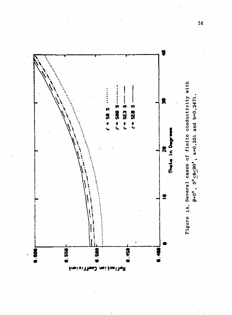
along the conductor. The results of a finite conductivity
are shown in Figure 18 where equation (58) has been included
in the iteration equation. The results resemble that given
by Jordan and Balmain [30] for a lossy ground and follow
the idea that the grid represents a shunt impedance. Over-
all, good agreement is obtained with previously computed and
measured results.
As a final note, some concern has been expressed over
the non-convergence of the iterative technique and over the
fact that increasing the number of Floquet modes not not in-
crease the accuracy of the solution [24] . The first con-
cern has been addressed in the preceeding sections while the
second will be addressed now. When an iterative equation is
in a non-convergent region, the solution may only be arriv-
ed upon by an accident of computation unless special methods
of computation have been included.
The consequence of adding additional Floquet modes is
adding additional points that are in the non-convergent re-
gion. The result of this consequence can range from produ-
cing a large variation in the iterated solution to helping
58
•H rtf> N•H ••P OO II3 J3
T3C T3O CO Oj
•p•HC•H<H
«HO
(00)
rt
f<
CM•
OIIoJ
v|OV|
oo
0) o> O0) II
CO O-•
QO
0)Pi3bo
59
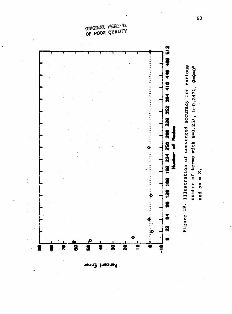
the iterated solution. The control over the results is nil
with a non-convergent iterative scheme. However, when the
contraction corrector method is applied, the expected in-
crease in accuracy with increasing Floquet modes is obtain-
ed. Of course, a limit on accuracy still exists due to the
finite register length of the computing machine used. The
case of a X/4 cell width, X/600 radius wire with infinite
conductivity and $=0=0° is chosen to illustrate the above
comments. A plot of converged accuracy is shown in Figure
19. The usual leveling off accuracy is noted. This is due
to the higher order Floquet modes having less and less
effect on the solution, i.e., the farther away wires con-
tribute less and less to the fundamental cell when a con-
vergent process is used.
60
J l l i T I I f I f
. .
- • ' . . '
» ' . -
'
.
- >^ ^• <8 -•
* . —
• «•'
o -
o -_J±
A, *i ' I Ai i" i i i i f
u>
*V«D
^
5W
W»*r
s.ffi 4» xN £X<9 k.o» ^w •
•siW|Ni«
8S
s8s«»
CD
o•Hhcd>
tio
«H
>,Ocd»H
oocd
•o0)bo»H
0)>Coo
«H0
Co•H+Jcdu>1 %+JCO3iHpH»-t
•OrH
0)^3be•Hfo
oOIIo>II®-
•k
»<f.^<CM•
OII&
«f<mCM•
oIIcdJS•p•HS
CO
0)V
«Hot .M0)
X5
C
•CO
8
G
•oCed
61
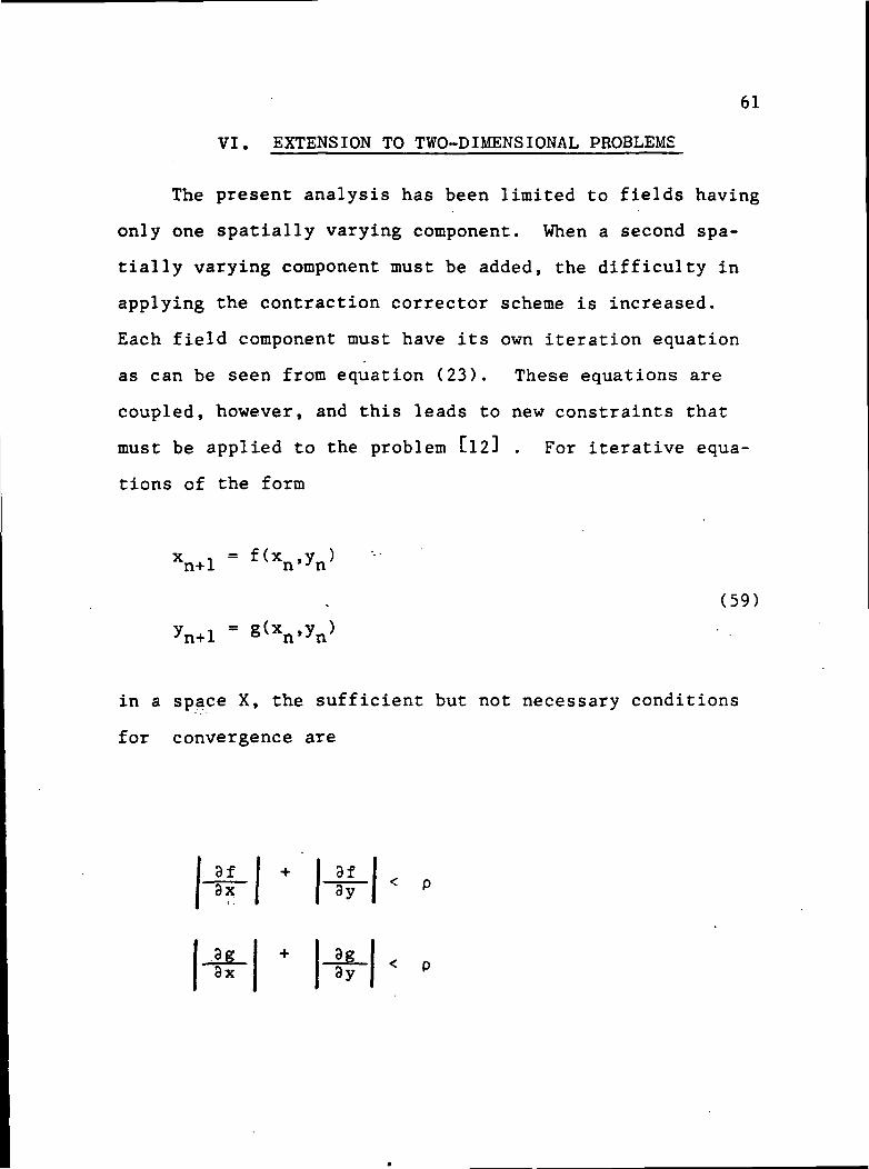
VI. EXTENSION TO TWO-DIMENSIONAL PROBLEMS
The present analysis has been limited to fields having
only one spatially varying component. When a second spa-
tially varying component must be added, the difficulty in
applying the contraction corrector scheme is increased.
Each field component must have its own iteration equation
as can be seen from equation (23). These equations are
coupled, however, and this leads to new constraints that
must be applied to the problem Cl2l . For iterative equa-
tions of the form
xn+l
(59)
in a space X, the sufficient but not necessary conditions
for convergence are
9f + 8f13T -57
_ _ .8x 3y
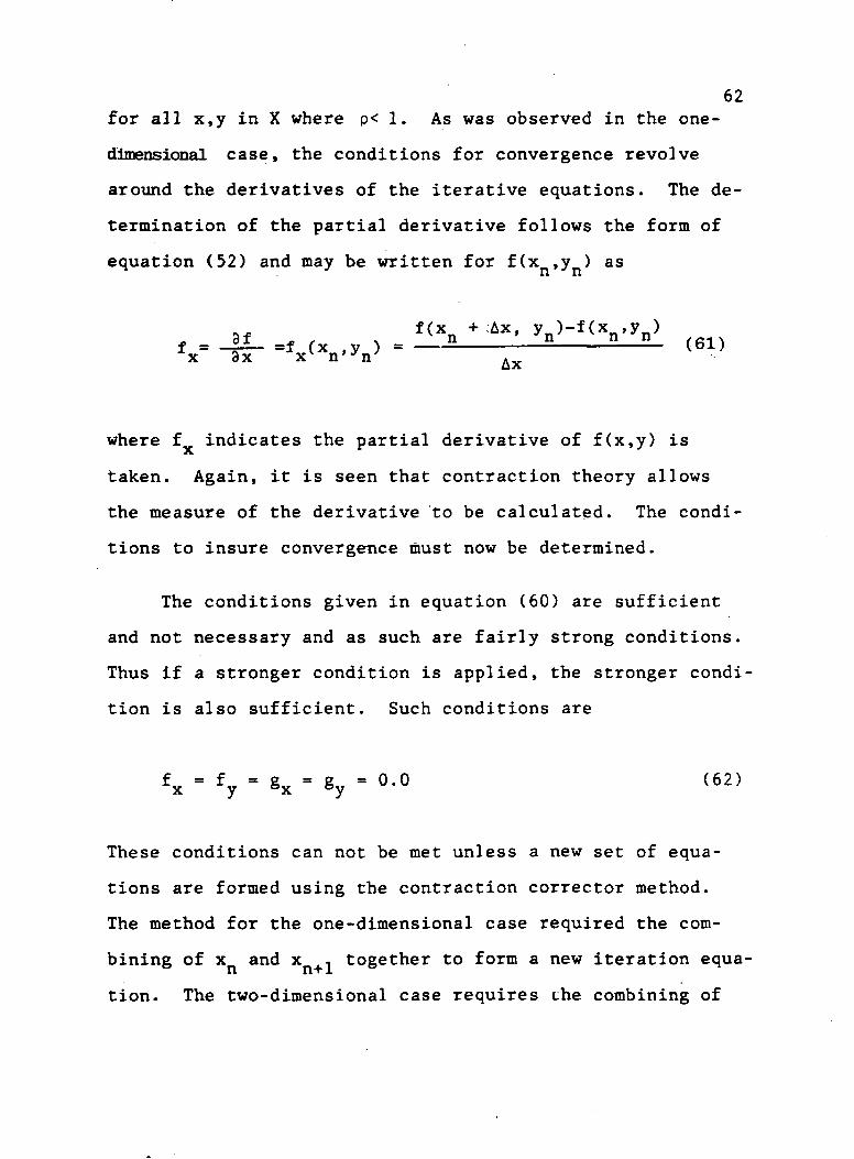
62for all x,y in X where p< 1. As was observed in the one-
dimensional case, the conditions for convergence revolve
around the derivatives of the iterative equations. The de-
termination of the partial derivative follows the form of
equation (52) and may be written for f(x ,y ) asn n
Ax' yn)"f(xn'yn)
where f indicates the partial derivative of f(x,y) isJv
taken. Again, it is seen that contraction theory allows
the measure of the derivative to be calculated. The condi-
tions to insure convergence must now be determined.
The conditions given in equation (60) are sufficient
and not necessary and as such are fairly strong conditions.
Thus if a stronger condition is applied, the stronger condi'
tion is also sufficient. Such conditions are
• fy ' Sx ' 6y - 0.0 (62)
These conditions can not be met unless a new set of equa-
tions are formed using the contraction corrector method.
The method for the one-dimensional case required the com-
bining of x and x , together to form a new iteration equa-
tion. The two-dimensional case requires the combining of
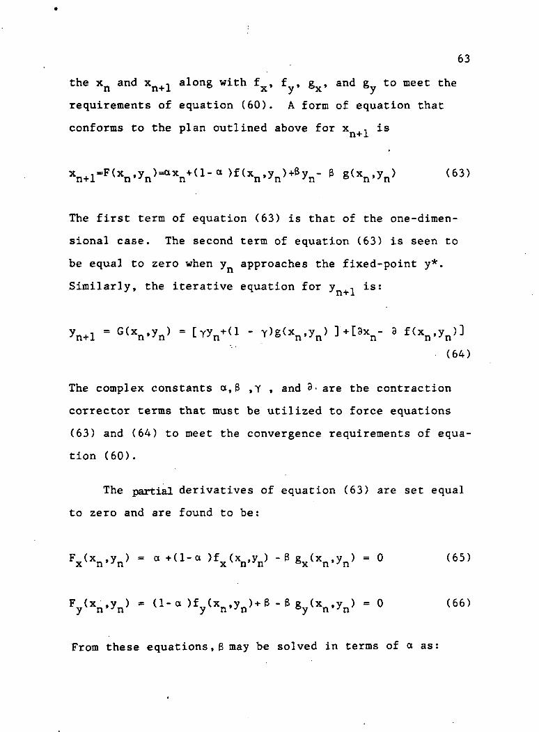
63
the x and x , along with f , f , g , and g to meet then n * x x y x y
requirements of equation (60). A form of equation that
conforms to the plan outlined above for x +, is
-a >f (xn- V+6>V B S(xn-V (63)
The first term of equation (63) is that of the one-dimen-
sional case. The second term of equation (63) is seen to
be equal to zero when y approaches the fixed-point y*.
Similarly, the iterative equation for y +, is:
V ^[3xn- 9 n
(64)
The complex constants a, 3 ,Y * and 3- are the contraction
corrector terms that must be utilized to force equations
(63) and (64) to meet the convergence requirements of equa-
tion (60).
The partial derivatives of equation (63) are set equal
to zero and are found to be :
(65)
yw * (1-<"Wyn)+6-'iy*n,yn> -From these equations, (3 may be solved in terms of a as
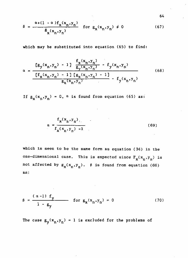
64
1 -a)fx(xn»yn:g (x ,y )x n n
which may be substituted into equation (65) to find:
a = Y " " (68)
If g (x ,y ) =0, a is found from equation (65) as:x TI n
a = (69)
-1
which is seen to be the same form as equation (34) in the
one-dimensional case. This is expected since F (x ,y ) isx n n
not affected by g (x ,y ). 6 is found from equation (66)A il II
as:
( a -1) f
1 - g y
for gx(xn,yn) = 0 (70)
The case g,,(x ,y ) = 1 is excluded for the problems ofy n ' n r
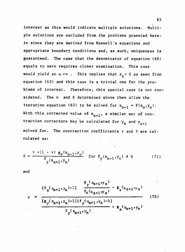
654
interest as this would indicate multiple solutions. Multi-
ple solutions are excluded from the problems prsented here-
in since they are derived frotn Maxwell's equations and
appropriate boundary conditions and, as such, uniqueness is
guaranteed. The case that the denominator of equation (68)
equals to zero requires closer examination. This case
would yield an a •*» . This implies that x = 0 as seen from
equation (63) and this case is a trivial one for the pro-
blems of interest. Therefore, this special case is not con-
sidered. The a and $ determined above then allow the
iteration equation (63) to be solved for x , = F(x ,y ).n+l n J n
With this corrected value of x +, , a similar set of con-
traction correctors may be calculated for y and y
solved for. The contraction coefficients y and 3 are cal-
culated as:
Y +(1 - Y) gw(x^,1 ,y3 --
and
~ gx(xn+l'yn)
(72)
66
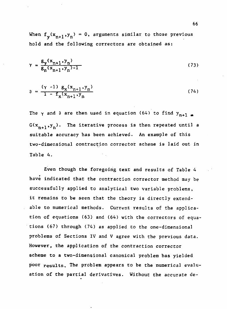
When f (xn+i»yn) = 0» arguments similar to those previous
hold and the following correctors are obtained as:
(73)
(74)
The Y and 9 are then used in equation (64) to find
G(x ,,y ). The iterative process is then repeated until a
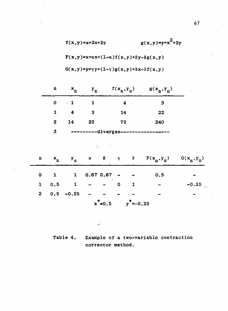
suitable accuracy has been achieved. An example of this
two-dimensional contraction corrector scheme is laid out in
Table 4.
Even though the foregoing text and results of Table 4*
have indicated that the contraction corrector method may be
successfully applied to analytical two variable problems,
it remains to be seen that the theory is directly extend-
able to numerical methods. Current results of the applica-
tion of equations (63) and (64) with the correctors of equa-
tions (67) through (74) as applied to the one-dimensional
problems of Sections IV and V agree with the previous data.
However, the application of the contraction corrector
scheme to a two-dimensional canonical problem has yielded
poor results. The problem appears to be the numerical evalu-
ation of the partial derivatives. Without the accurate de-
67
f(x,y)=x=2x+2y g(x,y)=y=x2+2y
F(x,y)=x=ax+(l-a)f(x,y)+By-$g(x,y)
G(x,y)=y=yy+(l-Y)g(x,y)+Sx-3f(x,y)
n
0
1
2
3
xn
1
4
14
yn
1
3
22
rHv«
^n'V
4
14
72
«<VV
3
22
240
n XQ yn a B y 9 F(xu ,yn) G(x n ,y n )
0 1 1 0.67 0.67 0 . 5
1 0.5 1 - - 0 1 - -0.25
2 0.5 -0.25 -
x =0.5 y =-0.25
Table 4. Example of a two-variable contraction
corrector method.
68
termination of f , f , g , and g , it is doubtful the con-x y x y
traction corrector method will be successful in arriving at
a convergent solution. Another problem that is not readily
apparent is the stringent conditions placed on the partial
derivatives. Invoking such strong conditions as given in
equation (60) may cause computational problems and eased or
adjusted conditions may be necessary uo reach a viable so-
lution method. These problems are being investigated and
useful results are expected in the near term [25] .
The usefulness of the two-dimensinal contraction cor-
rector can not be underestimated. For instance, when a
plane wave strikes a one-dimensional grating at an inci-
dence angle that induces :current along two axes, a cross-
polarized scattered field will be generated. The two-
dimensional nature of the problem must be addressed to ob-
tain the valuable cross-polarized information. The solu-
tion for reflection of waves from actual mesh surfaces is
also of interest and involves the use of the method de-
tailed in this dissertation.
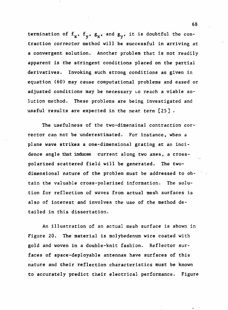
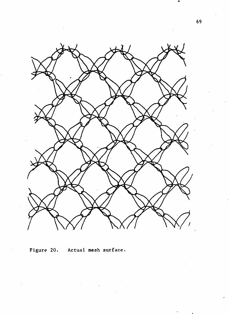
An illustration of an actual mesh surface is shown in
Figure 20. The material is molybedenum wire coated with
gold and woven in a double-knit fashion. Reflector sur-
faces of space-deployable antennas have surfaces of this
nature and their reflection characteristics must be known
to accurately predict their electrical performance. Figure
69
Figure 20. Actual mesh surface.
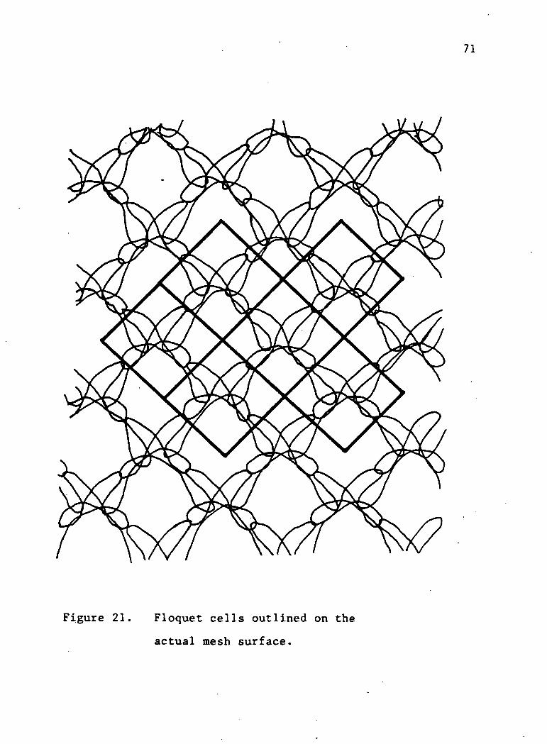
70
21 illustrates the periodic nature of the mesh surface. It
can be seen from the outlined boxes that Floquet cells may
be formed. This periodic nature may be capitalized on and
used to formulate the mesh surface into a suitable problem
for the contraction corrector scheme.
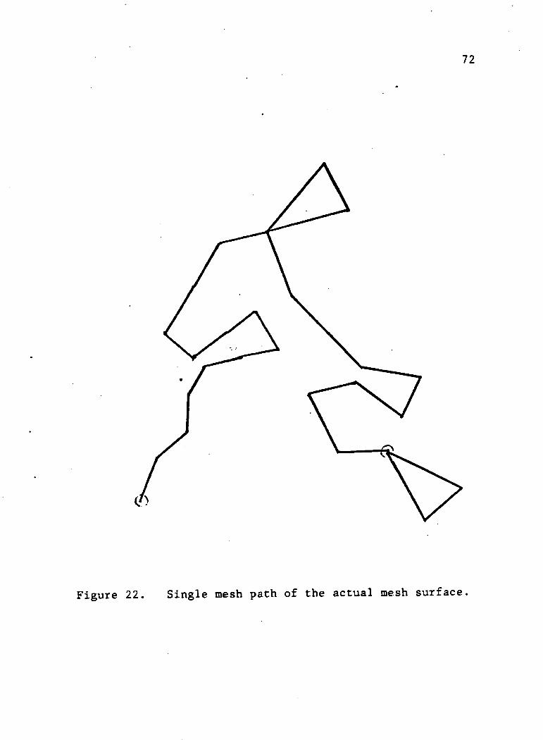
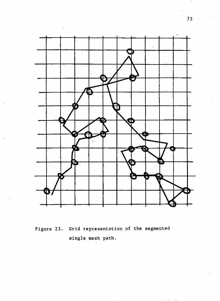
Figure 22 is the discrete representation of one single
mesh path. The discretation of the mesh path is accomp-
lished with twenty-eight, approximately equal length,
straight segments. With these segments defined, it is pos-
sible to overlay a grid onto the segments to achieve a rep-
resentation of the mesh surface. The equally spaced points
on the grid represent the sampled points required for the
Fourier Transform of the solution method. This typical
grid representation of the mesh surface will allow the de-
termination of the reflection characteristics of the sur-
face. Other surface weaves and materials may be placed on
similar grids and their reflection characteristics calcu-
lated. Figure 23 illustrates the application of the grid
to the segmented single mesh path.
71
Figure 21. Floquet cells outlined on the
actual mesh surface.
72
Figure 22. Single mesh path of the actual mesh surface
73
Figure 23. Grid representation of the segmented
single mesh path.
74
VII. CONCLUSIONS
A new method called the contraction corrector method
has been developed to insure the convergence of the one-
dimensional spectral-iteration approach when solving elec-
tromagnetic scattering problems. The method was presented
beginning with basic examples of the iterative method and
progressing to detailed iterative operator theory. Comput-
ed data generated from the scheme was critiqued and compar-
ed to work previously presented and was found to agree well,
The ability to predict the regions of solvability with the
contraction corrector scheme was demonstrated. The method
was then utilized to solve for the reflection coefficients
from an infinite grating of thin wires and the results were
compared to previously published data. The ideas of gener-
alization to a two-dimensional problem were discussed. A
solution technique for the two variable contraction cor-
rector method was developed and numerical difficulties in
applying the method were discussed. A sketch of an actual
mesh surface was presented and the application of the spec-
tral-iteration approach was detailed. A general reference
list and an over-view of both the k-space problem formula-
tion and the spectral-iteration approach were also included.
The material presented in this dissertation gives a
solid foundation for future research, and indicates that a
75suitable method for analyzing scattering from arbitrary
mesh surfaces can be developed. The recommendations for
future research should be directed toward understanding the
the shortcomings of the two-dimensional problem as detailed
in Chapter VI. With the proper constraints placed on the
two-dimensional problem and the correct evaluation of the
partial derivatives, a suitable method of solution is deemed
obtainable. Another alternative is the reformulation of
the problem with another method of attack. Many numerical
methods have yet to be applied to the problem and one may
will be suited for the two-dimensional scattering problem.
76
REFERENCES
[1] G.G. Macfarlane, "Surface impedance of an infiniteparallel wire grid at oblique angles of incidence,"IEE, No. 93, Part III A, pp. 1523-1527, 1946.
[2] J.R. Wait, "Reflection at arbitrary incidence from aparallel wire grid, "App. Sci. Res., Section B, vol.4, pp. 393-400, 1954.
[3] R.E. Collins, Field Theory of Guided Waves, McGraw-Hill, New York, 1960.
[4 ] R.B. Kiebuntz and A. Ishimaru, "Scattering by a peri-odically apertured conducting screen," IRE Trans. Ant.and Prop., vol. AP-9, pp. 506-514, Nov. 1961.
[5] N. Amitay and V. Galindo, "The analysis of circularwaveguide phased arrays," BSTJ, pp. 1903-1932,Nov. 1968.
[6 ] C.C. Chen, "Transmission through a conducting screenperforated periodically with apertures," IEEE MTT,vol. MTT-18, pp. 627-632, Sept. 1970.
[7 ] S.W. Lee, "Scattering by dielectric-loaded screen,"IEEE Trans. Ant. and Prop., vol. AP-19, pp. 656-665,Sept. 1971.
[8 ] J.P. Montgomery, "Scattering by an infinite periodicarray of thin conductors on a dielectric sheet," IEEETrans. Ant. and Prop., vol. AP-23, No. 1, pp. 70-75,January 1975.
[9 ] C.M. Tsao and R. Mittra, "A spectral-iterationapproach for analyzing scattering from frequencyselective surfaces," IEEE Trans. Ant. and Prop., vol.AP-30, No. 2, pp. 303-308, January 1982.
[10 ] N.N. Bojarski, "K-space formulation of the electro-magnetic scattering problem," Tech. Rep. AFAL-TR71-75, March 1971.
[11 ] J.C. Brand and J.F. Kauffman, "Analytic considerationsfor calculating the complex reflection characteristicsof conducting mesh antenna surfaces," Int. Sci. RadioUnion, Albuquerque, NM, May 1982.
[12 ] S.D. Conte and C. DeBoor, Elementary NumericalAnalysis, McGraw-Hill, New York, 1972,.pp.-44 - 50.
77
[13 ] R.F. Harrington, Time-Harmonic Electromagnetic Fields.McGraw-Hill, New York, 1961, pp. 27 - 347 y« - 100.
[14 ] V. Galindo and C.P. Wu, "Numerical solutions for aninfinite phased array of rectangular waveguides withthick walls," IEEE Trans. Ant. and Prop., vol. AP-14,No. 2, pp. 149-158, March 1966.
[15] A.B. Carlson, Communication Theory, McGraw-Hill, NewYork, 1975, pp. 56 - 58.
[16 ] W.M. Patterson, Iterative Methods for the Solution ofa Linear Operator Equation in Hilbert Space-A survey,Lect.Notes in Math, 394,Springer-Verlag, New York,1974.
[17 ] M. Altraan, Contractors and Contractor DirectionsTheory and Application, Marcel Dekkar, New York, 1977.
[18] I. Stakgold, Green's Functions and Boundary ValueProblems. John Wiley, New York, 1979, PP. *** -zo9.
[19] A.V. Oppenhiem and R.W. Schaffer, Digital SignalProcessing, Prentice-Hall, Englewood Cliffs, NJ,1975, Chapter 3.
[20] M.I. Astrakan, "Averaged boundary conditions on thesurface of a lattice with rectangular cells," Radioand Elec. Phys., No. 8, pp. 1239-1241, Aug. 1964.
[21 ] J.C. Brand and J.F. Kauffman, "The application ofthe spectral-iteration approach to conducting meshreflector surfaces," Int. Sci. Radio Union, Houston,TX, 1983.
[22] E.G. Jordan and K.G. Balmain, Electromagnetic Wavesand Radiating Systems, Prentice-Hall, EnglewoodCliffs, NJ, 1968> pp. 144 - 150.
[23] S.A. Schelkunoff, Electromagnetic Waves, Van Nostrand,New York, 1943, pp. 264.
[24] J.P. Mongtomery, "Analysis of frequency selectivesurfaces using the spectral-iteration approach,"Int. Sci. Radio Union, Houston, TX, 1983.
[25] C. Christodolou, J.C. Brand, and J.F. Kauffman, tobe published.
[26] R. Mittra, W. Ko, Y. Rahmat-Samii, "Transform approachto electromagnetic scattering," Proc. IEEE, vol. 67,No. 1, pp. 1486-1503, Nov. 1979.
[27] M. Kontorovich, V. Petrun'Kin, N. Yesepkina, and 78
M. Astrakhan, "The coefficient of reflection ofa plane electromagnetic wave from a plane wire mesh,"Radio Eng., vol. 7, pp. 222-231, 1962.
[28 ] R.F. Harrington, Field Computation by Moment Methods,Reprinted by Roger F. Harrington, Cazenovia, New York,1968, pp. 127 - 131.
[29] R.F. Harrington, Time-Harmonic Electromagnetic Fields,McGraw-Hill, New York, 1961,pp. 223 - 225.
[30] E.G. Jordan and K.G. Balmain. Electromagnetic Wavesand Radiating Systems. Prentice-Hall, EnglewoodCliffs, NJ, 1968, PP. 629 - 635.
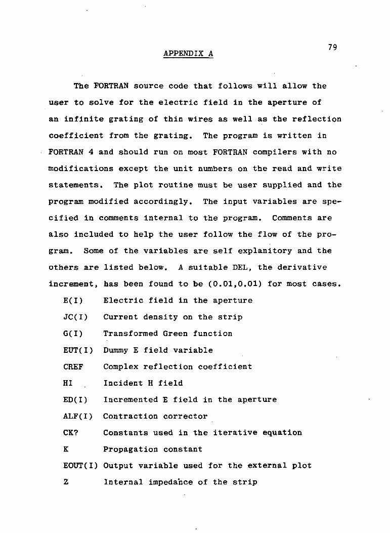
79APPENDIX A
The FORTRAN source code that follows will allow the
user to solve for the electric field in the aperture of
an infinite grating of thin wires as well as the reflection
coefficient from the grating. The program is written in
FORTRAN 4 and should run on most FORTRAN compilers with no
modifications except the unit numbers on the read and write
statements. The plot routine must be user supplied and the
program modified accordingly. The input variables are spe-
cified in comments internal to the program. Comments are
also included to help the user follow the flow of the pro-
gram. Some of the variables are self explanitory and the
others are listed below. A suitable DEL, the derivative
increment, has been found to be (0.01,0.01) for most cases.
E(I) Electric field in the aperture
JC(I) Current density on the strip
G(I) Transformed Green function
EUT(I) Dummy E field variable
CREF Complex reflection coefficient
HI Incident H field
ED(I) Incremented E field in the aperture
ALF(I) Contraction corrector
CK? Constants used in the iterative equation
K Propagation constant
EOUT(I) Output variable used for the external plot
Z Internal impedance of the strip
80
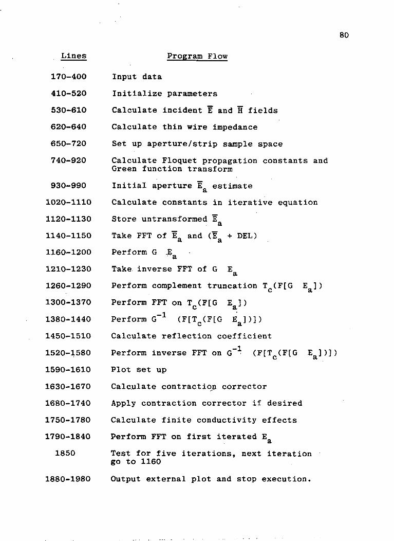
Lines
170-400
410-520
530-610
620-640
650-720
740-920
930-990
1020-1110
1120-1130
1140-1150
1160-1200
1210-1230
1260-1290
1300-1370
1380-1440
1450-1510
1520-1580
1590-1610
1630-1670
1680-1740
1750-1780
1790-1840
1850
Program Flow
Input data
Initialize parameters
Calculate incident E and H fields
Calculate thin wire impedance
Set up aperture/strip sample space
Calculate Floquet propagation constants andGreen function transform
Initial aperture E estimate3.
Calculate constants in iterative equation
Store untransformed EaTake FFT of l"a and (E& + DEL)
Perform G JE£t
Take inverse FFT of G EaPerform complement truncation T (F[G E ])
C 3.
Perform FFT on T (F[G E ])C £L
Perform G"1 (F[T (F[G E ])])C £L
(F[T (F[G El)])C £L
Calculate reflection coefficient
Perform inverse FFT on G~
Plot set up
Calculate contraction corrector
Apply contraction corrector if desired
Calculate finite conductivity effects
Perform FFT on first iterated E81
Test for five iterations, next iterationgo to 1160
1880-1980 Output external plot and stop execution,
PAGE S3Of POOR QUALFTY gl
CC****** F INAL .S **** D E R I V A T I V E C O R R E C T * * * * * *C Author Jerry C* Brznri
D A T E August 12, I^^SAl l rights rese rved
Dirension all arraysC O M P L E X E C 5 1 ? ) , J C ( M 2 > « G ( 5 1 i : ) f E U T ( 5 i ; ) , D E LCOMPLEX PI,CPEF,HICOMPLEX ED(512),ALF(51?),F9If £(512),U1(512) ,E[)UT(5^2)COMPLEX J»CK1(512) ,CK2(5U),CK(512),7DIMENSION ? O U T ( 5 1 2 t I D f ? )R E « L K ,K2
A = Floquet cell dimensionF = Strip size
WRITE(6,*) * INPUT FLOQLET CELL SIZE , STRIP SIZE'URITP(6,*) ' NORMA11TED IN WAVELENGTHS*R£AD(5,*)A,B
FREQ = Freauency in HertzWRITE«5,*) * INPUT F=>EQUENCy IN H£PT?'
MA> = FFT s i2e = Number of sair .cLes per ce l lIW = l O y S C ^ A X ) ; i.e. ^ A X = ? * * 1 UIP = 0 NO clct; IP = 1 »»lot ;NOTE..,,. External plot routine requiredIAC = C No correction;IA!>=1 Contraction corrector scheme applied
WRITE(6,*) 'INPUT ^f LOfaZCN), PLOT OPTION, ADJUST OPTICN*R£AD(5,*> ""AX, IW, IF,!A!i
SIP s Conductance cf stripUAITE(6,«) * INPUT C O N D U C T A N C E OF ST»IP IN SIE-ANS*READC5,*) S1G
TH = Theta angle of incidenceDEL = Comple» increment useo ir derivative routinePH = Phi angle o* Incicence
WRITE(6,*> * INPUT TH£TA ANGLE, DERIVATIVE DELTA, PHI ANGLE'48? Rt*CK 5,*)TH , DEL,PH
URITE(6,<»6) DEL16 F09MATC-',' DEL= ',iE10.4)
2 9 0 FORMATC-',' A D J U S T M E N T U S E DC Initialize routine constants
TPlsPI*2.C*2,997956?+8
ETAsSQRTfUU/FP)ITER=CJ=(D.C,1 .3)
«>D=18C./D1
C Calculate incident electric and magnetic field componentsC for electric field p a r a l l e l to hires, i.e. no cross-
C COlarirat ion includec oiatr^M*. ^I F f P H . L T . 4 5 . ) E I N C » 1 . C J2 ^ l PASEIS
IF fPH.GE.45. ) E I N C = C C S f T H - D S ) W TOOR QUALITYI F C P M . L T . 4 5 . ) S T H = C .IF fPH.GT.45. ) S T H = T H
H l s 1 . / E T A * f C O S ( T H » C R ) + J * S l N ( T H * D R ) )IF fPH.LT .45 . ) w : = 1 . / F T A « C O S ( T H * D P )Z = S Q R T f T P I * F R E O * U U / 2 . / S l G > * ( 1 . ? , 1 . 0 ) / T P I / 6W R I T 5 C 6 . 1 5 ) Z
15 F O R K A T f - * , ' Z = C , ? = 1 C . ? , - f - , E l 0 . 2 f - ) - )C Ca lcu la te number of s a m p l e s on strip and in aperture
NsIFlX(TAU/A*FLOAT(K*.X»
V AX1 = I»«X+1WRITEC6 f?3)
IF(NLGT.MAX) GOTOK=TPI/ALAMP
SK=K*SIN<TH*PR>*COS<°H*l,P)
C C a l c u l a t e Green funct ion t r a n s f o r mDO 4C ISI .^AX
U = T P I * ( I - 1 ) / A - S KG O T O 60
50 U = T P I * f I - M « X - 1 ) / A - S K
I F f U . G E . r 2 ) G C T O 7CG(I) = - J * 5 Q « ? T ( K 2 - U )G O T O 44
?C G(I)=-SQRTfU-K2)4A G(I) = G(D-SStf*SS*:/C(!)4C COK'TINUE
C Initial F fielC estimateDO 32C 1=1,NE(I)=(1.C,r.G)
32C EOCl)sF(I)*DELDO 22C I=N 1,»AXED(i)sCu.OtO.O)
C NOTE.... Iterative for« useo ir this program is x =C Calculate "BM ccrtion ct it e r a t i v e equation
DO 11C 1=1, MAX11C CK1 (I ) = HI*J«W*LU
CALL F F T C C K l t I W , « A X >DO 120 I=N1,»AX
12C CK?(I)=HI*W*UU/JDO IA'0 1=1 ,N
C A L L F F T C C I f 2 t I W , * » A X )DO 13C 1=1, MAX
13C C K ( l ) * ( C r 1 ( I ) - » C K ? ( ] » / 6 ( Z )
00 30C 1 = 1, P»X 833DC U1CI )=E(J)
CALL F F T ( £ D , IU ,MAX3CAIL F F T < E , I U , P ! A X )
Pecin "AX" portion of i t e ra t i ve equationPerfor iB (6*E)80 00 10C 1 = 1, M«X
E O C 1 ) « C O N J G < E D C I > * C C I ) )10C E ( I ) s C C N J G < E ( I ) * G < I ) >Ferfori" inverse t r a n s f e r * ol (G*E)
CALL F F T ( E , I W , M A X )CALL FFT (ED , IW,M*X )W R I T E (3,199) ITER
19S F O R M M C I C X t H O )P e r f o r m t runcat ion opera t i on T ( 6 * t >
00 150 1=1 ,NE D < I ) = C Q . O , C . O )
15C E( I)=(C. 0,0.0)DO 16C I=N1,PAXED C I ) = C O N J P (?D (I)) / M ^ XF.(I) = C C N J G C E < I ) ) / M * X
Ca l cu la te current dens i ty on str ip16C JC(I) = F ( ! ) * J /W/UU-HPer form inverse t r ans fe r * en T ( G * t )
C A L L F F T ( £ , I W , ^ A X )CALL FFT<ED,IW,MAX)
Perform TCG*E)/G and acd constant trO"DO 17C 1 = 1, M«X
EUT(Z)*CCNJG(E<2))/KAX17C CONTINUECalculate reflection cce^ficiert
P I = J * S I N ( S T H * D R ) / C C S ( S T H * L P )
A53 FO«?MAT(6X,* «EF= * , Fl u. = , cGx , 'CRE F= ' , F1 0. 2 ,1 X , F1 C .C Perfcrir irverse t r ansf c r^at ion to obtain first iteratedC electric field
CALL FFTCEUT, IU fPA>)CALL FFT<EPU T»I«,M*X)DO 2CC J =1 ,M«XEDUTCI)=CONJG(EDUT<1))
20C EUT(I) = CONJG<EUT(D)C Flct option
IFClP.LT.Cn GOTO 150CALL JBPLOT (?UT ,l« A ) ,TT t K , tCuT )
180 ITER=IT£P+1C Call subroutine to calculate derivative of operator andC contraction factor
CALL DF3IV(EUT,EDUf ,"AX ,PR IN E , AL F , I AD , D£L ,CO^ )WRITE (6t3iD) CON
34C FOfiMAT(/,1^X,* CON1R«CTICN = *vFlu.^)C Perfcr* ccrrecticn on electric tield; NCT£... If l«D=u
JDRIGINAL'PAGFISC ro adjustment is usec as A L F ( 1 ) = 0 . 0 ^ POOR QUALITY 84
00 350 1=1,N
E U T ( I ) * A L F ( X > * U 1 C X ) * < 1 . - » L F ( X ) ) * E U T C I )
35C EDUTCI)*EUT(I>+DEL310 CONTINUE
C Ca lcu la te f ield on str ip due to f ini te conduct iv i ty00 21C I«Nl t*AXE D U T < I ) = - J C ( T ) * 2 * B
C Perfcr i r t r ans fo rm of E f ie lc tc begin next i terat ionCALL FFT (EUT , IW,« IAX)C A L L F F T ( E D U T , I U , M A X )00 220 I=1 f P»XED(I )=EDUT(I )
2 tC E( I )=EUT( I )I F C 1 T E P . G T . 5 ) G O T O 2<-CG O T O 6C
24C C O N T I N U EDO 777 I=1,M«XP I N D E X = F L O ' T ( I - 1 ) / F L O A T ( V A X - 1 ) * A
C P e r f o r m plot f t r c t i cns 1f-r e x t e r n a l Plot rout ineW R ! T E ( ? 2 , 7 ? f i ) P I N D E X , E O U T C I , 1 , 1 ) , E O U T ( I , 2 f 1 ) , £ O U T ( I , 3 t 1 )
* ,ECUT<1, A , 1 ) f E O U T ( ] , r , 1 )WRITE(23,77£) SINDEX tEOUTU,1,?i,LOUT I I,2,2),EOU*(1,3 , 2)
+ ,ECUT<If4f?),EOUT( I,',2)77F FORMAT(6F8.2)777 CONTINUE
2 6 C F O P K A T C - ' t l T X , * T I * I L Y E X I T * )?9 f W R ! T E ( 6 , ? 9 )? 9 FORM«T( * - * , * E R R O R I N W )
999? S T C PENSSUPROUTIME J °PLOT(* , INT , i T E R t t o u T )COMPLEX «(1)DIMENSION *^P(512) ,EOUT(512,10,2),PHASE(512)N=ITER*1DO 8C J=1,INTAMP(1 ) = C*BS(«(!))
*II»AG(A (I) J
IF(ARS(PHX).LT.I.E-2:) FHX=1.t-2n
PHASE(I)=57.295*AT#NZ(PHY,PHX)EOUT(I,N,1)=AKP(I)EOUT( I,N,2)=PH«SE(1)
80 CONTINUERETURNENDSURROUTINE DERIVCE ,EP,MAX,PKlH5,ALF,IAD,OEL,CON)
C This subroutine calculates tht derivative andC contraction factor ol the operator
COMPLEX E(r*AX) ,ED(rAy)«ALF rn«x) « PRlKF(r.AX) .DELCOK=C.C
PRIME (I)=(FD(D-E(l)?/ntLCOK=CCN+fC*BS(PRIMf(!)*D'L))*"2
85
13 IF(!*D.LT.1> ALF(I)«~.n'CON= SORT (COM FLO AT C M A X > >/C«faS(DEL)RETURNENDSUBROUTINE F F T C A f H f N )
C This is the FFT subroutine tailed from the main programCOMPLEX A(K)fUty,T
j=r00 7 Is1,N«"1IF(I.6E«J) GOTO 5T=»(J)A(J)*ACX>A(I)=T
5 K=NV26 IF(K.GS.J) GOTO ?
GOTO e7 J=J+K
DO 20 L=1t"LE=2**LLE1=LE/E
DO 2? J = 1,I.E1DC 1C I«JtK,L£
7=A(IP.)*UA(IP)=A(!)-T
10 «(I)=A(I)*Tao u=u*w
END
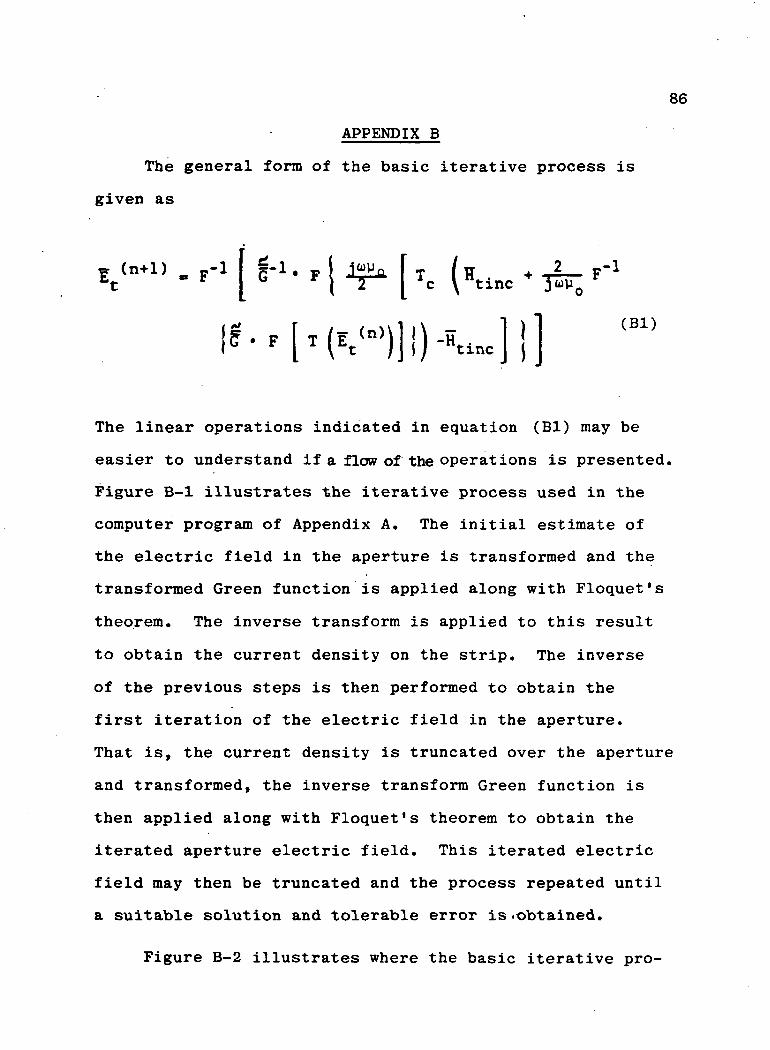
86
APPENDIX B
The general form of the basic iterative process is
given as
(n+1) -.-I
The linear operations indicated in equation (Bl) may be
easier to understand if a flow of the operations is presented.
Figure B-l illustrates the iterative process used in the
computer program of Appendix A. The initial estimate of
the electric field in the aperture is transformed and the
transformed Green function is applied along with Floquet's
theorem. The inverse transform is applied to this result
to obtain the current density on the strip. The inverse
of the previous steps is then performed to obtain the
first iteration of the electric field in the aperture.
That is, the current density is truncated over the aperture
and transformed, the inverse transform Green function is
then applied along with Floquet's theorem to obtain the
iterated aperture electric field. This iterated electric
field may then be truncated and the process repeated until
a suitable solution and tolerable error is-obtained.
Figure B-2 illustrates where the basic iterative pro-
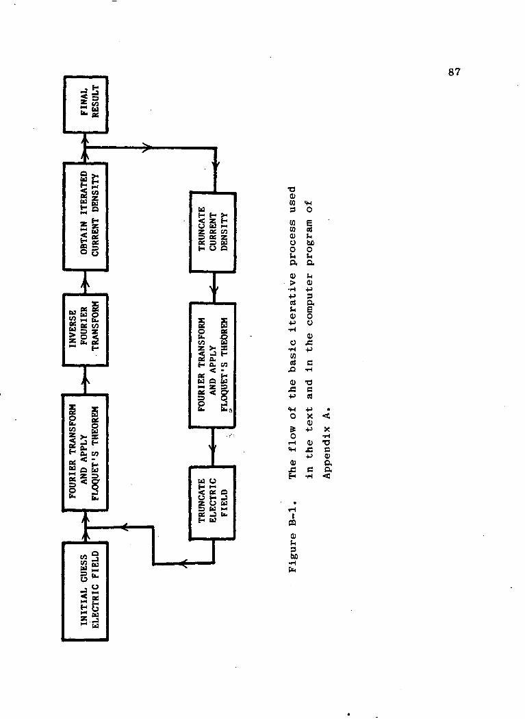
87FI
NA
LR
ESU
LT
*s|u £fc Q
OB
TAIN
1
CURR
ENT
uTR
UN
CAT
CURR
ENT
DEN
SITY
1
NV
ER
SE
I
^
£CO
iH
g•4
ae§tb
FO
UR
IER
1
RA
NS
FOR
M I
fr-
\51
gPO. CO
O U
5I(b
^^N_ Q
CO j
is§*•d2< ae
£ &9 W
£.JM u
igw
fsae£z >• s
sss 1 -tj ft. fft
K *u a u
|<"
>
•
^fl
r
U UH )->< Q- o0 j- J§ e> u
U Mae J u.H U
•a0CO9
COCO0O
0)(HbO
a a0 JH
•H -P•P ?as a>4 E0 o•P o
u x:•H -pCO<& c
•acrt
«HO
0)
tH
CO
0
bD•Hf>H
•pX0•p0
X•H•ac0aa
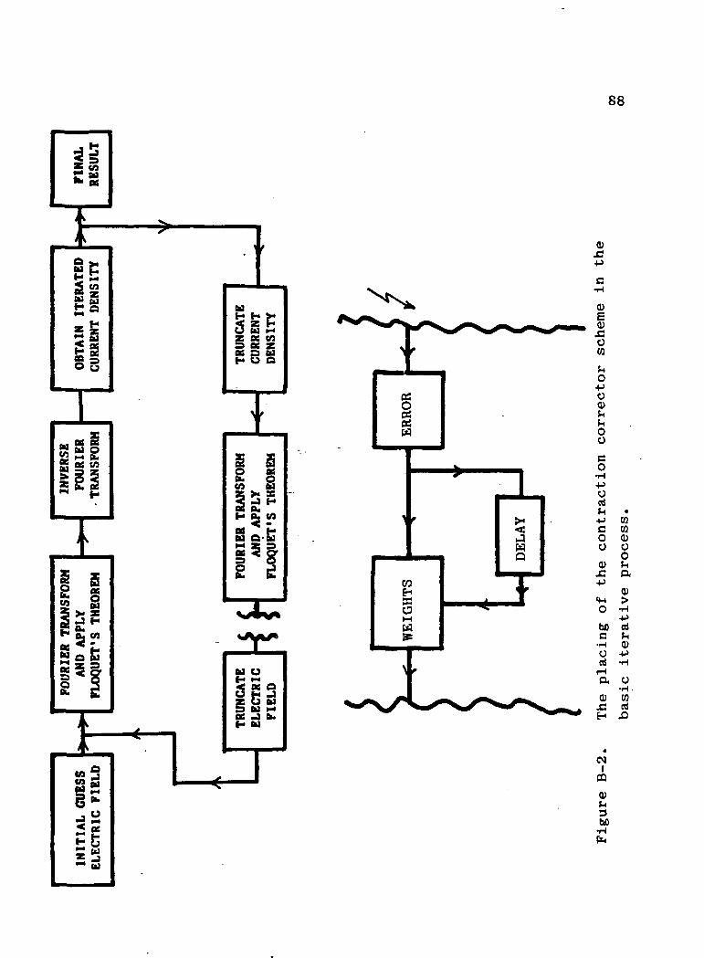
88
^s
at
*iiglH4
Z zi £
II
«
1
[NV
ER
SE
FO
UR
IER
RA
NS
FOR
M
" H
, I,i s2 gto 55 ^ £*" a* ca08 rsitS 25x g
i«°SS w» •-
B **
^2< eeEC« w* -3••« M
M
Hi
fr
iEg ee en
06 Zat p MH O C
>
ssto
^
S§Z >• X^C PM
) H
M O. CA
«^LM Q-OUM Z Sg 5 &
JW4
§
1k^
»^
M UH ••4
: o
1 Mat -3 b.H M
0)JC•p
CSl
CQ
3bD
89
cess may be interupted to accomodate the contraction cor-
rector scheme. This point is chosen since an iterated
solution has been generated. With this iteration and any
previous iterations a filtering process may be employed.
The text pointed out the usefulness of the contraction
corrector scheme since it guarantees a convergent solution.
Thus, the iterative process can be viewed as a feedback
process whereby the errors of processing can be eliminated
and a useful solution of the problem obtained.
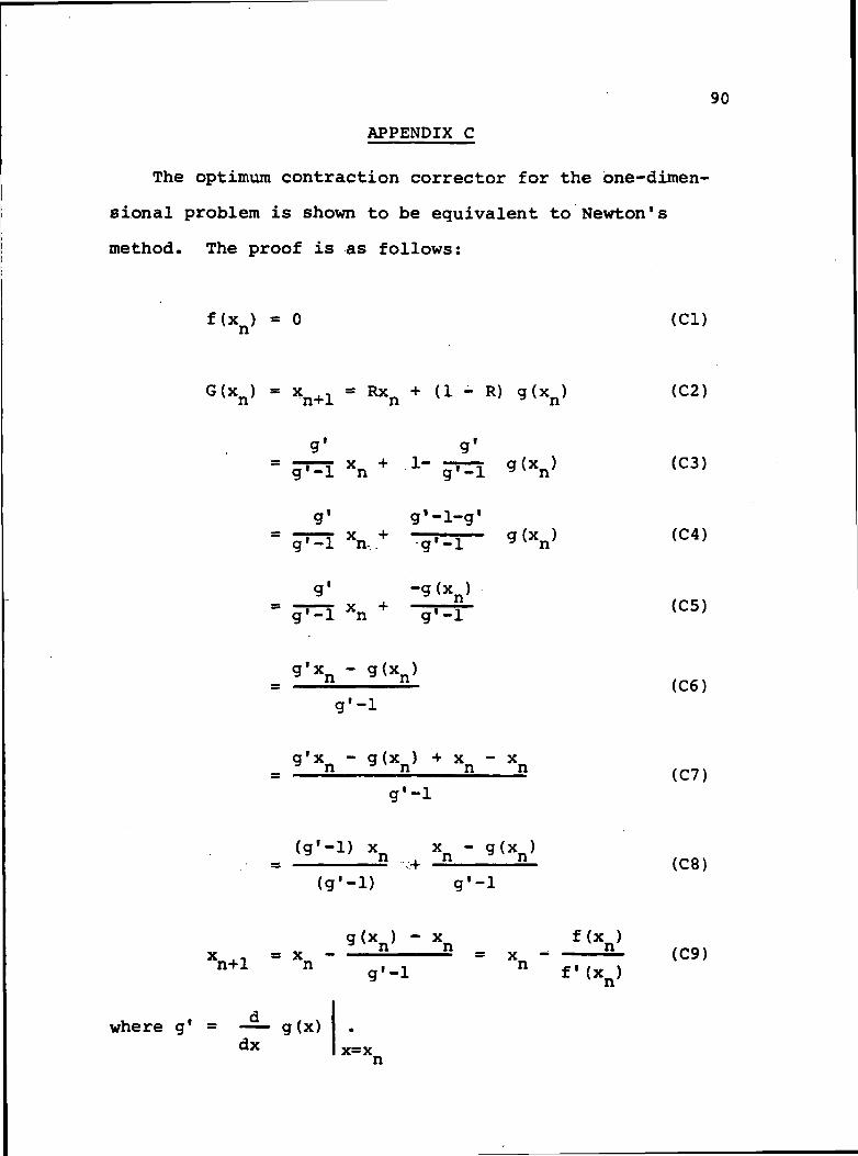
90
APPENDIX C
The optimum contraction corrector for the one-dimen-
sional problem is shown to be equivalent to Newton's
method. The proof is as follows:
f(xn) = 0 (Cl)
G(xn> - xn+l
g'
- R) g(xn)
g'
<C2)
(C3)
g' g'-l-g'x +
g1
n, g'-l
-g(xn)n + g'-l
(C4)
(C5)
g'-l(C6)
g'xn - g(xn)
g'-l(C7)
xn . xn -
(g'-l) g'-l(C8)
" xxn+l = xn *
n
g'-lx -n
where g1 = — g(x)dx x=xn
(C9)