NASA-CR-203326

SYSTEM SYNTHESIS IN PRELIMINARY AIRCRAFT DESIGNUSING STATISTICAL METHODS n

Mr. Daniel DeLaurentis

NASA Multidisciplinary Analysis Fellow

Dr. Dimitri N. Mavris

Assistant Professor & Associate Director ASDL

Dr. Daniel P. SchrageProfessor & Co-Director ASDL

Aerospace Systems Design Laboratory (ASDL)School of Aerospace Engineering

Georgia Institute of Technology;

./,// i / ,, _.J ./- ....

,ti/ 0 (.' ' ' _

U-J<5 ' ;-'/'/

Abstract

This paper documents an approach to conceptual and earlypreliminary aircraft design in which system synthesis isachieved using statistical methods, specifically Design ofExperiments (DOE) and Response Surface Methodology(RSM). These methods are employed in order to moreefficiently search the design space for optimumconfigurations. In particular, a methodologyincorporating three uses of these techniques is presented.First, response surface equations are formed whichrepresent aerodynamic analyses, in the form of regressionpolynomials, which are more sophisticated than generallyavailable in early design stages. Next. a regressionequation for an Overall Evaluation Criterion is constructedfor the purpose of constrained optimization at the systemlevel. This optimization, though achieved in a innovativeway, is still traditional in that it is a point designsolution. The methodology put forward here remedies thisby introducing uncertainty into the problem, resulting insolutions which are probabilistic in nature. DOE/RSM isused for the third time in this setting. The process isdemonstrated through a detailed aero-propulsionoptimization of a High Speed Civil Transport.Fundamental goals of the methodology, then, are tointroduce higher fidelity disciplinary analyses to theconceptual aircraft synthesis and provide a roadmap fortransitioning from point solutions to probabilistic designs(and eventually robust ones).

I. Introduction

Over the past few years, a significant amount ofresearch has taken place on the topic of how to efficientlydesign complex aerospace systems, especially as historicaldatabases (once the centerpiece of conceptual design)

become increasingly obsolete. This obsolescence hasresulted from departures from traditional products(configurations outside historical databases, changingmissions and functionalities, etc.) and processes(manufacturing methods, information exchange, etc.).

I Presented at the 20th Congress of the International Councilof the Aeronautical Sciences, Sorrento. Italy. Sept. 8-13, 1996.

This connection of product and process characterizationsform the heart of Integrated Product and Process Design(IPPD). To truly achieve the "Integrated" part of IPPD.numerous groups have been conducting research under thegeneral term of Multidisciplinary Design Optimization(MDO). MDO has been defined as "'A methodology lotthe design of complex engineering systems that aregoverned by mutually interacting physical phenomena andmade up of distinct interacting subsystems". '_' One of theearliest and most well known approaches to executingMDO was through the Global Sensitivity Equations(GSE) approach, where "what if" questions are answer_through so-called system sensitivity derivatives whichrelate a system response to changes in design variables.including the interactions of the disciplines involvedExamples are seen in References 2 and 3, though there arenumerous others. Reference 4 provides an excellentsurvey of recent work and current tools being utilized b)MDO researchers.

So a key to successful MDO is developing means tointelligently analyze these systems ,_'ith mutuallyinteracting phenomena. The strength of the GSE lies inthe determination of interactions betw, een disciplines in astructured and logical manner. These interactions.represented as sensitivities, can then bc used as gradientinformation in a traditional optimization exercise. TheGSE approach, though, provides only local gradientinformation and some of the derivatives max be difficult

to calculate. Further, the point design paradigm is stillemployed. Thus, others, including the authors inReference 5, have used the GSE approach incombination/coordination with other techniques and toolsin an attempt to improve the prt_ess and give moreinsight to the designer. However, for conceptual levelvehicle synthesis, with numerous interacting disciplines.many design variables (both continuous and discrete), andoften times large deviations from the baseline, an effective

and comprehensive methodology has not emerged.This paper de_ribes new developments which form

the initial execution of an evolving IPPD approach,providing a potential solution to this mcthodologx need.The approach puts vehicle synthesis in its proper role of

https://ntrs.nasa.gov/search.jsp?R=19970009400 2018-05-04T19:39:29+00:00Z

the integrator of the mutually interacting disciplines.Traditional sizing and synthesis is generally performedwith first order tools due to the impracticability ofconnecting complex codes together into an iterative sizingcode. The use of statistical techniques in the proposedmethod allows for more flexibility in searching a designspace by representing large amounts of knowledge (e.g.complex, expensive analysis codes or physicalexperiments) via response surface equations (RSEs).Caveats in the use of statistical approximations in thereplacement of complex analysis include accuracy andscope issues. How well the fitted equations represent thegiven data will be important in determining the validity ofthe results. Also. the RSEs are valid only in the designspace (multidimensional region bounded by the rangeextremes for each design variable considered) for whichthey were formed. These issues will be revisitedthroughout the remainder of this paper.

So then, the approach put forward here addresses amultidisciplinary problem (the synthesis of an aircraft)from an IPPD perspective, where the recompositionportion of synthesis is executed using Design ofExperiments (DOE) and the above mentioned RSEs.These techniques allow for the introduction of moreaccurate contributing analysis into the synthesis andsizing process. RSEs have been used in the aerospacefield over the past several years by several groups. _''7_'_A key development presented here, however, is that asystematic plan for incorporating RSEs directly into avehicle synthesis code as "model" equations has beendeveloped. This process is demonstrated by modeling themission aerodynamics (i.e. vehicle drag as a function ofplanform shape, overall geometry, and flight condition)via RSEs. incorporating these RSEs into a synthesiscode. and then using this modified code to conduct asystem level optimization. The key objective at thesystem level is affordabilit3'.

Finally. the last step of the approach involves therecognition that aircraft design is not truly deterministic innature. Uncertainties, in a variety of forms, existthroughout the design sequence. Thus, a framework forcreating probabilistic solutions is presented whichtransitions from the point design solution to one in theform of a distribution.

II. IPPD Approach to System Recomposition

IPPD specifically brings together design andmanufacturing considerations. Designing aircraft in anIPPD (and Concurrent Engineering) framework could beviewed as designing with a focus on affordability, whichimplies an understanding of how the various discipline,mission, design, and economic variables affect thefeasibility ("can it be built") and viability ("should it bebuilt") of an aircraft. The Georgia Tech IPPDmethodology can best be viewed as a recompositionprocess, employed once the various paris of the problemhave been broken down and analyzed. In order to do thisrecomposition in an meaningful way, Product and Processdesign variables and constraints must be consideredsimultaneously. Product characteristics arc those thatpertain directly to the subject of product design, such as

geometry, materials, propulsion systems, etc. Processcharacteristics, on the other hand, refer to those items

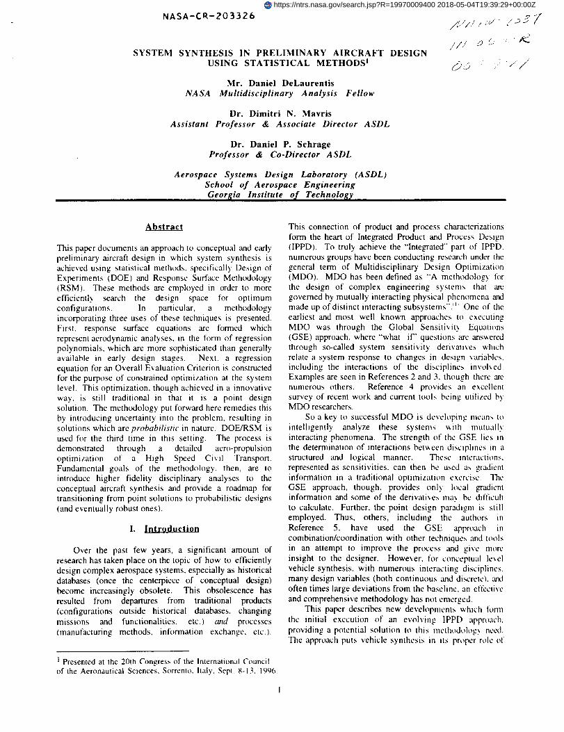
related to how the product is designed, produced, andsustained over its lifetime. A rational approach toexecuting the integration process takes the form of a"Funnel", as illustrated in Figure 1.

Product F ea_ ible C o n_igll rail on P rool_s

Figure 1: Systematic Recomposition-Implementing IPPD for Affordability

In essence, the Funnel represents a concurrentrecomposition process in which all of the variousdisciplinary interactions, ideally, arc accounted for during"synthesis", or recomposition. For this study, theaerodynamic and propulsion disciplines were examined indetail, and structures considerations being limited tocomponent weight estimation based on historical damcompiled in the sizing code FLOPS (FLight OPtimizationSystem) _''. The first level in the funnel representsfundamental design variables in each category. These arethe parameters available to the engineer in formulatingconfigurations. The importance of the next level, theintroduction of RSM, lies in two facts. First, it allows

the formation of response equations which can be used toreplace complex simulation codes needed to arrive at apoint design optimum. Second, as is illustrated at the

bottom of the figure, once economically viablealternatives are synthesized, these RSEs can be used toobtain the discipline metrics, such as L/D or SFC, whichcorrespond to the optimal configuration. After theequations are formed, this discipline level information is

used to perform system synthesis (with appropriateconstraints) through the use of a synthesis ct_c. What isthus obtained arc the various design variable settingswhich correspond to the point design optimum (i.e. oneaircraft configuration) and a corresponding $/RPM value.The $/RPM (average required yield per Revenue Passengcr

Mile)is theselectedOverallEvaluationCriterion(OEC)forcommercialaircraft.Thismetricimplicitlyrepresentstheticketprice,onapermilebasis,thatanairlinemustchargeinordertoachieveaspecifiedreturnoninvestment(ROI) It alsoaccountsfor a requiredROI for themanufactureroftheaircraft.

Unfortunately,thisoptimalOECresultcanneverbeachievedexactly due to economic factors which thedesigner cannot control, such as market and airlineconsiderations. These economic factors introduce

uncertaint 3' to the design process resulting in adistribution for $/RPM. This distribution, or moreprecisely its characteristics (such as mean and variance for

a normal distribution), is subsequently used to determineif economic viability has been achieved based on a the

needs of the airline and manufacturer. If not, a designiteration (see Figure 1) is necessary.

The need for disciplinary approximations becomesevident in Figure 1, as the connection of complicatedanalysis tools (e.g. CFD for aerodynamics, FEM forstructures, cycle analysis for propulsion, etc.) from eachdiscipline would be impractical. Common designvariables, if they exist, between areas can be represented asnoise factors in the formation of particular RSEs. Forexample, the position of the engine nacelles, a decisiongenerally made by the structures and propulsion andengineers, is kept as a variable in the aerodynamic modelequation formation. A brief review of the fundamentals ofDOE/RSM is presented next. More detailed informationcan be obtained from numerous references?"_"_ J_.,t2,,_4_

III. Design of Experiments andthe Response Surface Method

Understanding the characteristics of the design spaceand behavior of the proposed designs as efficiently aspossible is as important to the designer as finding thenumerical optimum. This is particularly true for complexaerospace systems which require multidisciplinaryanalyses, a large investment of computing resources, andintelligent data management. As an alternative to standard

parametric approaches to design space search and complexiterative optimization routines, the DOE/RSM applicationdeveloped here appears to have several advantages. Beforeapplying the methods, the following paragraphs outlinethe fundamentals of DOE/RSM.

The (RSM) comprises a group of statisticaltechniques for empirical model building and exploitation.By careful design and analysis of experiments, it seeks torelate a response, or output variable, to the levels of anumber of predictors, or input variables. In most cases,

the behavior of a measured or computed response isgoverned by certain laws which can be approximated by adeterministic relationship between the response and a setof design variables; thus, it should be possible todetermine the best conditions (levels) of the factors to

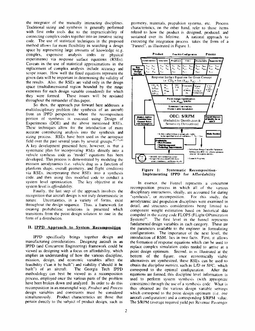
optimize a desired output '_'. Unfortunately, many timesthe relationship between response and predictors is eithertoo complex to determine or unknown, and an empiricalapproach is necessary to determine the behavior. Thestrategy employed in such an approach is the basis of theRSM. In this paper, a second degree model of the selected

responses in k-variables is assumed to exist. A notionalexample of a second order model is displayed in Figure 2for two variables xl and x2.

Figure 2: Second Order Response Surface Model

The second degree RSE takes the form of:

k k k

R=b,, + Zb,,,, + Zb,,x, 2+ ZZb,,x,,,,i_l i=1 I<l

where, bi are regression coefficients for the first degree

terms, bii are coefficients for the pure quadratic terms, bijare coefficients for the cross-product terms (second c_rderinteractions), and b,, is the intercept term. To facilitate thediscussion to follow, the components of equation (I) arcfurther defined. The x i terms are the "main effects", the

xi z terms are the "quadratic effects", and the x_xj are the"'second-order interaction terms".

Since it is in a polynomial form (though other formsare possible, e.g. exponential or logarithmic, through atransformation of both the independent and dependentvariables), the RSE can be used in lieu of more

sophisticated, time consuming computations to predictand/or optimize the response R. If one is optimizing onR, the "'optimal" settings for the design variables areidentified (through any number of techniques) and aconfirmation case is run using the actual simulation codeto verify the results. Since the RSE is a regression curve,though, a set of experimental or computer simulated datamust be available.

One organized way of obtaining these data is theaforementioned DOE, which is used to determine a table

of input variables and combinations of their levelsyielding a response value (but also encompasses otherprocedures, like Analysis of Variance). There are manytypes of DOEs. Table 1 displays a simple full factorialexample for three variables (or factors) at two levels, aminimum and a maximum (sometimes also described as "-1" and "+1" points).

Table 1: Design of Experiment Example for a

two-level, 23 Factorial Design '_1_

Faclor$

Run I 2 3 ResponseI ),_2 + _3 + )_4 + + )_5 + y,6 + + )_7 + + ).8 + + + ,_

Theresponsecanbeanyof avarietyof metrics(suchasthrust,drag,pitchingmoment,weight,etc,),whilethedesignvariablesandtheirrangesdefinethedesignspace.Fortheapproachin thispaper,thefactorsbecomeinputvariablesto theanalysiscode,whilethe responseisgenerallythedesiredoutputoftheprogram.

ThesamefullfactorialDOEapproachcanbeusedforvariablesatthreelevels, requiring more runs but obtainingmore information by going from a linear representation toa quadratic one. On the other hand, evaluation of allpossible combinations of variables at two or three levelsincrefises the number of cases that need to be tested

exponentially, and thus quickly becomes impractical. Infact, testing 12 variables at three levels, their two

extremes and a center point, would take a total of 531,441

cases for a 312 factorial design.

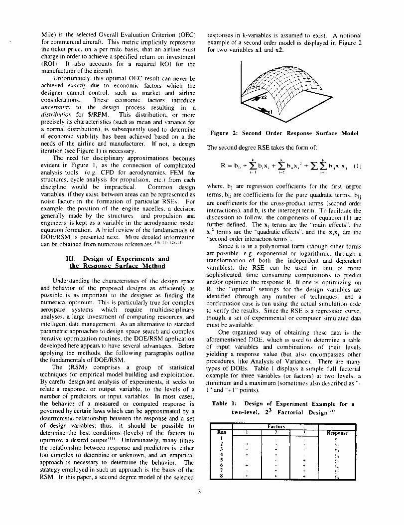
Table 2 illustrates that one way of decreasing thenumber of experiments or simulation runs required is toreduce the number of variables. But as Table 2 also

displays, a 37 full factorial design still requires animpractical 2,187 runs. Hence, fractional factorial andsecond order model designs (of which the CentralComposite is an example) are proposed as a moreplausible means to perform experiments. Table 2provides three examples.

Table 2: Number of Cases for Different DOEs ':_'

DOE

3-level,Full Factorial

Central

CompositeBox- Behnken

D-OptimalDesi[n

7 Varia-bles

2.187

143

62

36

12 Varia-bles

531.441

4,121

2.187

91

Equation

n

3

n

2 +2n+l

(n+l)(n+2)/2

Fractional factorial DOEs use less information to

come up with results similar to full factorial designs.This is accomplished by reducing the model to onlyaccount for parameters of interest. Therefore, fractionalfactorial designs neglect third or higher order interactionsfor an analysis (see RSE in Equation ( 1 )), accounting onlyfor main and quadratic effects and second order interactions.

Thus, a tradeoff exists in fractional factorial designs.The number of experiments or simulations (often referredto as "cases") grows as the increasing degree to whichinteraction and/or high order effects are desired to beestimated. Since generally only a fraction of the fullfactorial design number of cases can be run, high ordereffects and interactions are not estimable. They are said tobe confounded, or indistinguishable, from each other interms of their effect on the response. This aspect offractional factorial designs is described by their resolution.Resolution III implies that main effects are entirelyconfounded with second order interactions. Thus, one

must assume these interactions to be zero or negligible inorder to estimate the main effects. Resolution IV

indicates that all main effects are estimable, though secondorder interactions are confounded with other such

interactions. Resolution V or greater means that bothmain effects and second order interactions are estirnablc

(though for Resolution V designs, third order interactionswould be confounded with second order effects, hence must

be zero) _L''. The example presented in Section IV willemploy a Resolution V design for the RSEs.

Problems in aircraft design typically have many

design variables, complicating sizing and optimization.As a general approach in DOE/RSM, a first DOE isperformed in order to reduce the number of variables byidentifying the significant contributors to the response.This exercise, termed a "screening test", uses a two levelfractional DOE for testing a linear model, thus estimatingthe main effects of the design variables on the response.It allows for an investigation of a high number ofvariables in order to gain an initial understanding of theproblem and the design space.

A visual way to see the results of this screening isthrough a Pareto Chart _L_, displayed in Figure 3. Itidentifies the most significant contributors to the responsebased on the linear equation generated from the DOE data.Bars indicates which variables contribute how much while

a line of cumulative contribution tracks the total response.By defining the percentage of contribution desired, thevariables to be carried along to the RSE generation can bedetermined from the array of variables in the Pareto Chart.

Term

LF

S-Fuel

ROI-A

U-Comp

ProdQ

#Pax

E-TF

LC

ROI-M

U|d

R&S

LabRate

A-TF

Insur

TRT

Mamt

Scaled Eltlmate

-00242133

002019050

001529961

-00093494

-00082122

-00071229

0_90495

0,00495633000471449

-00046931

000347228

0.00252888

-00023878

000090584

000048753

0.00036315

Figure 3: Sample Pareto Chart - Effect of Design

Variables on the Response

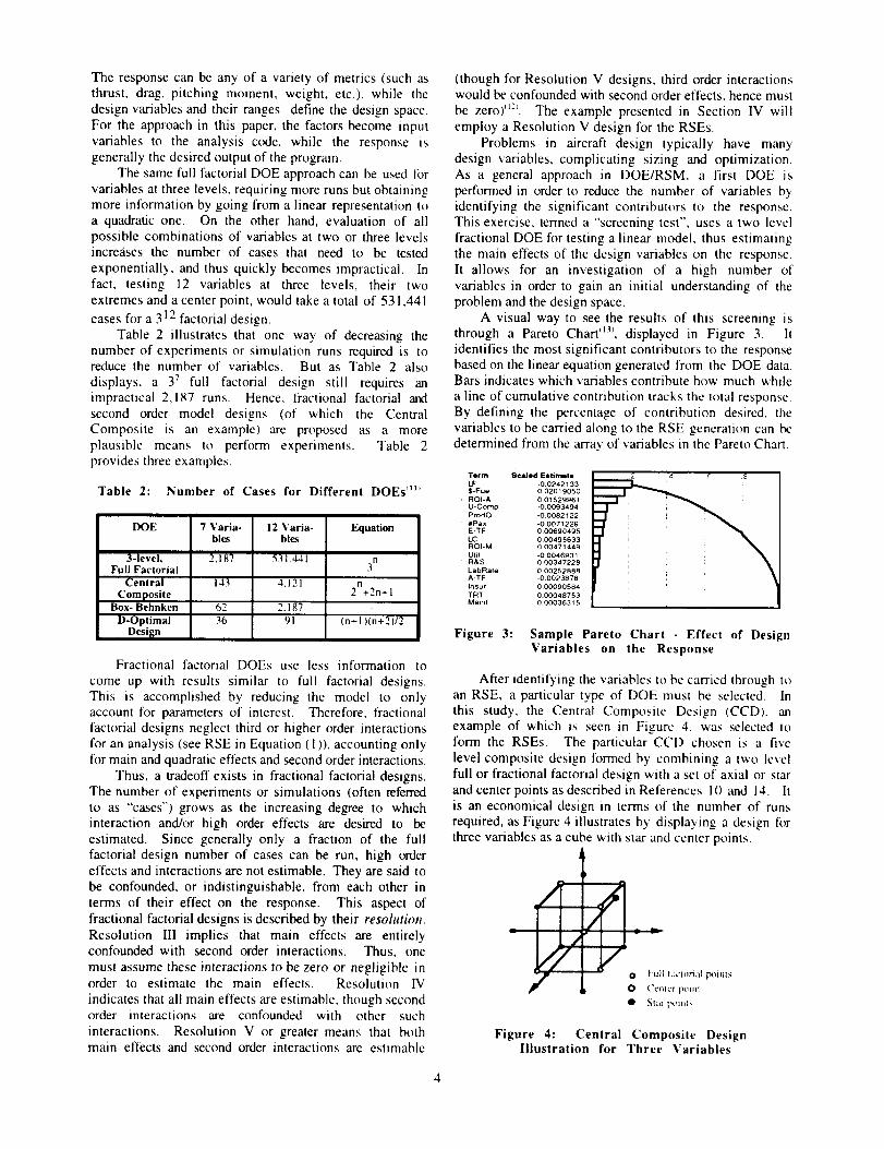
After identifying the variables to be carried through toan RSE, a particular type of DOE must be selected. Inthis study, the Central Composite Design (CCD). anexample of which is seen in Figure 4. was selected toform the RSEs. The particular CCD chosen is a five

level composite design fom_ed by combining a two levelfull or fractional factorial design with a set of axial or starand center points as described in References 10 and 14. Itis an economical design in terms of the number of runsrequired, as Figure 4 illustrates by displaying a design forthree variables as a cube with star and center points.

A L

0 Center point

• Star points

Figure 4: Central Cumposile DesignIllustration for Three Variables

Thedistancebetweenaxialpointsdescribestheextentof the designspace.The centerprovidesmultiplereplicates,for estimatingexperimentalerror,whichisassumednon-existentfor simulation-basedanalysis.Hence,justonereplicateisrequiredforthecenterpoint.

Finally,withtheCentralCompositeDesignin hand,anRSEcanbeobtainedbyusingEquation(1) asamodelfor regressionon thegenerateddata. Unlikefor trueexperiments,astatisticalenvironmentwithoutanyerrorcanbeassumed,sothatall deviationsfromthepredictedvaluesaretruemeasuresof a modelfit. A lackof fitparameterfor themodelexpresseshowgoodthemodelrepresentsthetrueresponse.A smalllackoffit parameterusuallyindicatesexistinghigherorderinteractionsnotaccountedforin themodel.Dependingon thelevelofthislackoffit,anewdesignwithatransformedmodeltoaccountfortheseinteractionsshouldbeused.

IV. Example:Aero-Propulsion Optimization for an H_;_T

With the IPPD method and accompanying DOE/RSMtools described, the approach is now demonstrated via anexample: synthesis and optimization of a High SpeedCivil Transport. Choosing a wing planform shape for asupersonic transport is a task that to this day is still along and tedious one. The need for efficient performanceat both sub- and supersonic cruise conditions exhibitimmediately the presence of conflicting design objectives.Studies by Boeing and Lockheed during the 1970's for theSuperSonic Transport (SST) program looked extensivelyat this issue'_M_% In brief, one resulting conclusion wasthat low aspect ratio, highly swept wings have low drag atsupersonic speeds (since the cranked leading edge serves toprovide subsonic type flow normal to the wing leadingedge). Unfortunately, such planforms are poor insubsonic cruise. The variable sweep wing option hadcomplications involving reduced fuel volume and weightand complexity penalties; thus this concept was neverseriously considered. The so-called double delta emergedas a compromise. Here the outboard panel helps retainsome subsonic performance while keeping acceptablesupersonic cruise efficiency "_'. The study carried out

presently employs a DOE technique which models andexamines planforms ranging from the pure delta (arrow) tothe double delta.

The trades involved in planform selection arecomplicated by other discipline considerations (e.g.propulsion) and the presence of design and performanceconstraints at the system level which are directly related tothe wing. The limit on approach speed, for example, ismostly a function of wing loading. Fuel volumerequirements impact the wing size and shape. Both ofthese issues become sizing criteria and both tend toincrease the wing in size. Of course, increased wing area

brings with it higher induced and skin friction drag.Terminal performance at takeoff and landing (especiallyfield length limitations) also present a challenge.Increasing the low speed aerodynamic performance of thcaircraft will reap benefits for noise control through reducedthrust and more modest climb rates. The HSCT will ne_

its maximum Ct. at takeoff, and the use of high liftdevices will play a major role in making that maximumas high as possible. For this study, a configuration offlap settings was selected for the baseline aircraft based onthe SST studies and the takeoff and landing polars weregenerated using the code AERO2S _'.

Problem Formulation

The problem consists of using the new techniquesoutlined in Sections II and III in synthesizing ardeventually optimizing an HSCT type aircraft for a givenmission. Improved aerodynamic procedures over what iscurrently available in the synthesis code FLOPS arcincorporated via RSEs. Next, an RSE for the overallobjective function ($/RPM) and several performanceconstraints are generated and a constrained, point designoptimal solution (using aerodynamic and propulsiondesign variables) is found. Finally, steps necessary forintroducing and accounting for economic uncertainty arcdescribed. The execution of this uncertainty exercise isdescribed in Reference 8, also for an HSCT.

Forming RSEs for Mission Drag

The goal of introducing RSEs is to replace theexisting drag calculation in the synthesis codc FLOPS.As FLOPS is executing the input mission profile, itrequires calls to an aerodynamics module for drag at thatfight condition (M. h. CL). Ordinarily FLOPSdetermines drag by one of three methods: internalcalculations (based on the EDET aero predictionprogram_'% externally generated drag table, externallygenerated polar equation. Considering the functional tbrmof the drag polar equation:

C D =CDo +k_ _ .C__ l 2 )

RSEs for Co,, and kz, are to be formed as a function ofdesign variables and operational Math number. Thus, thetotal drag for a given aircraft configuration will still bc a

function of Math number and C L as well as configuration

design variables.The first step in forming RSEs is to first conduct a

screening test. Even with the computational advantagesbrought by DOE, an excessive number of design variablescan make the RSE generation expensive/difficult (SecTable 2). The design variables which are to make up theRSE model for vehicle drag must be the ones which have

the most influence on the aerodynamic characteristics ofthe airplane. A screening test is designed to identify thesubset of design variables which contribute most to agiven response (i.e. the variables for which the responsehas the highest sensitivity). For all of the aerodynamic

analyses performed in this study, public domain toolswere used, including the Boeing Design and AnalysisProgram (BDAPt '_' lot supersonic drag due tO liftprediction and skin friction drag. WINGDES '_' foroptimum camber and twist, AERO2S '_'' for subsonic dr_due to lift. and AWAVE '2'' for fuselage area ruling.

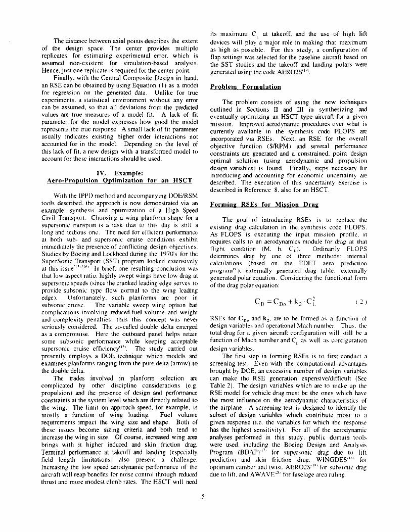
To begin the screening process, a parametric wing

planform definition scheme is selected which encompasses

the variety of wing shapes considered for a supersonic

transport, from a pure arrow wing to a kinked double

delta• A summary of all the design variables selected can

be found in Figure 5.

Other Design Variables ,_., x_,_gfor the Aerodynamic Screemn_. Planh_rmVariables

x_ln_ ( Normahzed b', _.¢1111-snan I

I/c al rot,t

• tic at tip

Nacelle Scahng

Hilrizont'.d Tail Area

CL DeszgnRI×II Alrfllil _ll_.' max th_ckn 1 t

Tip A/rlofl Ik',c max th,:kn I

Nacelle X-Iocath_n

WingRelerenceArea

,x_" t

Figure 5: Aerodynamic Design VariableSelection

Choosing meaningful ranges for the design variables

is critical. On the one hand, the ranges should be

somewhat large to include the largest design space

possible and increase the chances that the eventual optimal

configuration is captured. On the other hand. the range

must not be chosen so large as to reduce the prospects of a

good regression fit of the RSE to the actual highly non-

linear response. Additionally, there are physical

restrictions which limit the range choices. For example,

the wing at its aftmost location with longest root chord

must not interfere with the horizontal tail. Table 3 shows

a summary of all design variables with their chosen

ranges. Recall that planform variables are normalized by

span and their ranges are selected based on review of past

and present concepts. Variable "xwing" is normalized by

fuselage length. Note also that the screening test is a 2-

level (or linear) test. Since we are not interested in

forming an equation just yet, the linear sensitivities are

expected to do just as well in determining which are the

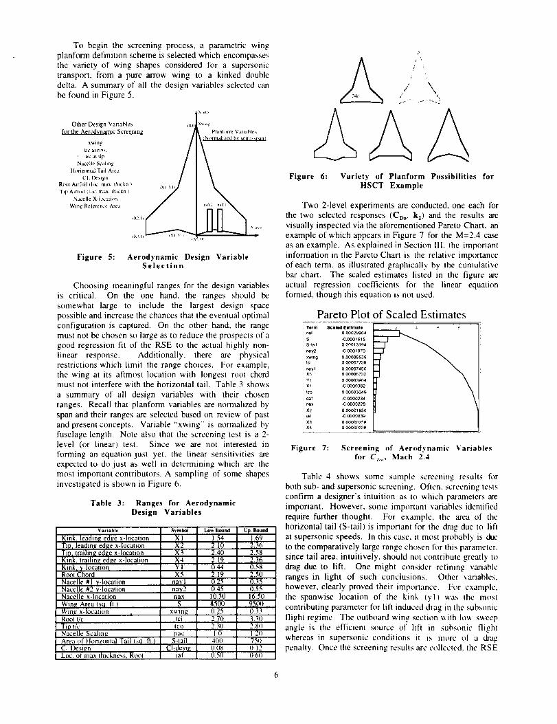
most important contributors. A sampling of some shapes

investigated is shown in Figure 6.

Table 3: Ranges for Aerodynamic

Design Variables

Variable Symbol Lo_ Bound Up. Bound

Kink_ leading edge x-location X I 1.54 1.69Tip, leading e, tge x-location X2 2.10 2.36Tip. trailing ecge x-location X3 2.40 2.58Kink_ trailing q'dge x-location X4 2.19 2.36Kink_ y-location Y 1 0.44 0.58Root Chord X5 2.19 2.50

Nacelle #1 y-location nayl 0.25 0.35Nacelle #2 y-location nay2 0.45 0.55Nacelle x-location nax 1030 16.50

Wing Area !sq ft / S 850t) 95(X)Wing x-location , xwing 0.25 0.33Rom t/c tci 2 7(1 3.3(tTip tic too 2.30 2.8(INacelle Scaling nac 10 120Area of Honzontal Tail tsq ft.) S-tail 4(1t) 750Cj Design CI-desig 008 0 12Loc of max Ihickness. Root iaf 0.50 060

/ \

Figure 6: Variety of Planform Possibilities forHSCT Example

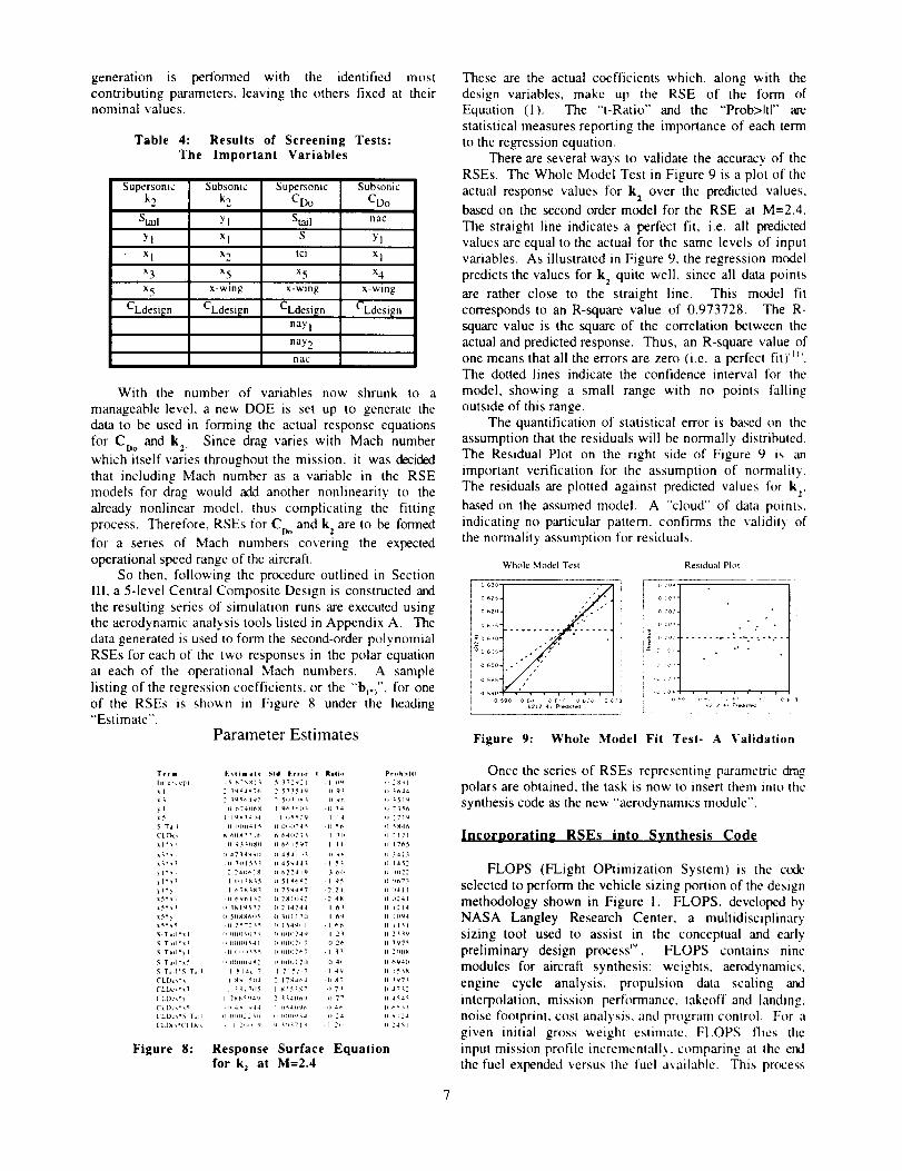
Two 2-level experiments are conducted, one each for

the two selected responses (CDo, k2) and the results are

visually inspected via the aforementioned Pareto Chart, an

example of which appears in Figure 7 for the M=2.4 case

as an example• As explained in Section III, the important

information in the Pareto Chart is the relative importance

of each term, as illustrated graphically by the cumulative

bar chart. The scaled estimates listed in the figure are

actual regression coefficients for the linear equation

formed, though this equation is not used.

Pareto Plot of Scaled EstimatesTerm Scakld ElUmate

hal 0 00029964

S -0.0001615S-tall 0 00013194

r_y'2 -0 0001070

xwlng 0 000085391el 0 00007739

nay1 0 00007450X5 0 00006732

Y 1 0 00003904

Xl -0 0000382

_co 0 00003049

oaf -0 0000234

nax -0 0000228

Y_. 000001856

_1 -0 0000039

x3 000000258

x4 0 00000038

Figure 7: Screening of Aerodynamic Variablesfor C I.... Mach 2.4

Table 4 shows some sample screening results fi_r

both sub- and supersonic screening. Often. screening tests

confirm a designer's intuition as to which parameters are

important. However, some important variables identified

require further thought. For example, the area of the

horizontal tail (S-tail) is important for the drag duc to lift

at supersonic speeds. In this case. it most probably is due

to the comparatively large range chosen fl_r this parameter.

since tail area, intuitively, should not contribute greatly to

drag due to lift. One might consider refining variable

ranges in light of such conclusions. Other variables,

however, clearly proved their importance. For example,

the spanwise location of the kink (vll was the most

contributing parameter lot lilt induced drag in the subsonic

flight regime. The outboard wing section with low sweep

angle is the efficient source of lift in subsonic l'light

whereas in supersonic conditions ii is more of a drag

penalty. Once the screening results arc collected, the RSE

generation is performed with the identified mostcontributing parameters, leaving the others fixed at theirnominal values.

Table 4: Results of Screening Tests:The Important Variables

Supersonic

k 2

Stall

Yl

x I

x 3

x 5

CLdesign

Subsonic

k 2

Yl

x I

x 2

x 5

x-wing

CLdesign

Supersonic

CDo

Stall

tci

x 5

x-wing

CLdesign

nay I

nay 2

nac

Subsonic

CDo

nac

Yl

x I

x 4

x-wing

CLdesi_n

With the number of variables now shrunk to a

manageable level, a new DOE is set up to generate thedata to be used in forming the actual response equations

for Coo and kz. Since drag varies with Mach numberwhich itself varies throughout the mission, it was decidedthat including Mach number as a variable in the RSEmodels for drag would add another nonlinearity to thealready nonlinear model, thus complicating the fitting

process. Therefore, RSEs for C_ and k z are to be formedfor a series of Mach numbers covering the expectedoperational speed range of the aircraft.

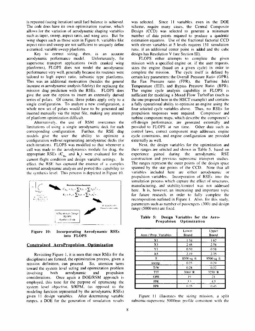
So then, following the procedure outlined in SectionIII, a 5-level Central Composite Design is constructed andthe resulting series of simulation runs are executed usingthe aerodynamic analysis tools listed in Appendix A. Thedata generated is used to form the second-order polynomialRSEs for each of the two responses in the polar equationat each of the operational Math numbers. A sample

listing of the regression coefficients, or the "b(._", for oneof the RSEs is shown in Figure 8 under the heading"Estimate".

Parameter Estimates

These are the actual coefficients which, along with thedesign variables, make up the RSE of the form ofEquation (1). The "t-Ratio" and the "Prob>ltt" arestatistical measures reporting the importance of each termto the regression equation.

There are several ways to validate the accuracy of theRSEs. The Whole Model Test in Figure 9 is a plot of the

actual response values for k 2 over the predicted values,based on the second order model for the RSE at M=2.4.

The straight line indicates a perfect fit, i.e. all predictedvalues are equal to the actual for the same levels of inputvariables. As illustrated in Figure 9, the regression model

predicts the values for k 2 quite well, since all data pointsare rather close to the straight line. This model fitcorresponds to an R-square value of 0.973728. The R-square value is the square of the correlation between theactual and predicted response. Thus, an R-square value ofone means that all the errors are zero (i.e. a perfect fit) '_'The dotted lines indicate the confidence interval for thc

model, showing a small range with no points fallingoutside of this range.

The quantification of statistical error is based on theassumption that the residuals will be normally distributed.The Residual Plot on the right side of Figure 9 is animportant verification for the assumption of normality.

The residuals are plotted against predicted values for k,,.

based on the assumed model. A "cloud" of data points,indicating no particular pattern, confirms the validity ofthe normality assumption for residuals.

Whole Model Test Residual Plot

o 63O , 0 00' .....

0 6_0- ," , _" 0 00.' '

06_" "'" 00c" ' •

O600- ." ,"

059O 06,:' ' _,_Io _tec, o_

Figure 9: Whole Model Fit Test- A Validation

T_rm

hllcr, upr

xl

xl

3,1

x5

S TJII

CLDc_

)l'x_

) ]'),I

xS'xI

_5")I

S Tall'xl

S Ta,I') ]

S Ta_'x_

CLDc,'_ I t 7_¢_5'_,.I'4

('LD_'_ T,IH () _+_HI_'/ &(*

l'i_lima|¢ Std I';rr.r

-5 M7",;4 i _ ;7292]

l 67_¢ _l 75_-I_7

_ (_(_,.14 _2 I_II_*]211

l _¢I_c ? 215¢ 7

! Rati,,

-o la

l 14

.() _

.ll

-2 21

-2 4_

16t

12_

(_ 26

.IJ 1_7

(171

_ 77

'r.h>lll

28ql

1644

7t5r,

271q

_84_

2121

I 7_5

1452

)2t4

2n_)H

.I?:C

24_

Figure 8: Response Surface Equation

for kz at M=2.4

Once the series of RSEs representing parametric dragpolars are obtained, the task is now to insert them into thesynthesis code as the new "'aerodynamics module".

Incorporating RSEs into Sv,¢h_sis Code

FLOPS (FLight OPtimization System) is the code

selected to perform the vehicle sizing portion of the designmethodology shown in Figure i. FLOPS, developed byNASA Langley Research Center, a multidisciplinary

sizing tool used to assist in the conceptual and earlypreliminary design process _. FLOPS contains ninemodules for aircraft synthesis: weights, aerodynamics,engine cycle analysis, propulsion data scaling ard

interpolation, mission performance, takeoff and landing,noise footprint, cost analysis, and program control. For agiven initial gross weight estimate, FLOPS flies theinput mission profile incremenlally, comparing at the endthe fuel expended versus the fuel available. This process

is repeated (sizing iteration) until fuel balance is achieved.

The code does have its own optimization routine, which

allows for the variation of aerodynamic shaping variables

such as taper, sweep, aspect ratio, and wing area. But for

wing shapes such as those seen in Figure 6, variables like

aspect ratio and sweep are not sufficient to uniquely define

a cranked, variable sweep planform.

Key to correct sizing, then, is an accurate

aerodynamic performance model. Unfortunately, for

supersonic transport applications (with cranked wing

planforms), FLOPS does not model the aerodynamic

performance very well, generally because its routines were

tailored to high aspect ratio, subsonic type planforms.

This was an additional motivation (besides the general

increase in aerodynamic analysis fidelity) for replacing the

mission drag prediction with the RSEs. FLOPS does

give the user the option to insert an externally derived

series of polars. Of course, these polars apply only to a

single configuration. To analyze a new configuration, a

whole new set of polars would have to be generated and

inserted manually via the input file, making any attempt

of planform optimization difficult.

Alternatively. the use of RSM overcomes the

limitations of using a single aerodynamic deck for each

corresponding configuration. Further, the RSE drag

models give the user the ability to optimize a

configuration without regenerating aerodynamic decks (foreach iteration)• FLOPS was modified so that whenever a

call was made to the aerodynamics module for drag. the

appropriate RSEs (Coo and k 2) were evaluated for the

current flight condition and design variable settings• In

effect, the RSE has captured the essence of a complex

external aerodynamic analysis and porled this capability to

the synthesis level. This process is depicted in Figure 10.

<1,

• , , _ ,

K 2 = b,, + '_ b+xl +'_bllx_ +

_4,,d,,'+,d fl r_t'_

A PrcIirn_nar} Design f

FLOPS

S,. nthcsls Cudc

was selected. Since !1 variables, even in the DOE

scheme, require many cases, the Central Composite

Design (CCD) was selected to generate a minimum

number of data points required to produce a quadratic

estimation equation. Use of the fractional factorial CCD

with eleven variables at 5 levels requires 151 simulation

runs, if an additional center point is added and the cubc

design has Resolution V (see Section III).

FLOPS either attempts to complete the given

mission with a specified engine or, if the user requests,

sizes the engine (based on a given cycle) in order to

complete the mission. The cycle itself is defined by

certain key parameters: the Overall Pressure Ratio (OPR),

the Fan Pressure ratio (FPR), the Turbine Inlet

Temperature (TIT), and Bypass Pressure Ratio (BPRI.

The engine cycle analysis capability in FLOPS is

sufficient for modeling a Mixed Flow TurboFan (such as

the one proposed here in the HSCT example) and contains

a fully operational ability to optimize an engine using the

four selected cycle variables above. Thus, no RSEs for

propulsion responses were required. Compressor and

turbine component maps, which describe the component's

off-design performance, are generated externally and

provided to FLOPS at run time. Other data such a.s

control laws, correct component map addresses, engine

cycle constraints, and engine configuration are provided

externally as well.

Next, the design variables for the optimization and

their ranges are selected and shown in Table 5, based on

experience gained during the aerodynamic RSE

construction and previous supersonic transport studies.

The ranges represent the outer points of the design space

spanned by the star points of the CCD. Note that all

variables included here are either aerodynamic or

propulsion variables. Incorporation of RSEs into the

simulation process which capture the effect of structures,

manufacturing, and stability/control was not addre_,_ed

here. It is, however, an interesting and important topic

for future research, in order to fully complete the

recomposition outlined in Figure 1. Also, for this study.

parameters such as number of passengers (300) and design

range (5000 nm) are fixed.

Table 5: Design Variables for the Aero-Propulsion Optimization

Figure 10: Incorporating Aerodynamic RSEsinto FLOPS

_on_trained AeroPropulsion Optimization

Revisiting Figure 1, it is seen that once RSEs for the

discipline(s) are formed, the optimization process, given a

mission definition, can proceed. So, attention turns

toward the system level sizing and optimization problem

involving both aerodynamic and propulsion

considerations. Once again a DOE/RSM approach is

employed, this time for the purpose of optimizing the

system level objective, $/RPM, (as opposed to the

modeling function represented by the aerodynamic RSEs)

given 11 design variables. After determining variablc

ranges, a DOE for the generation of simulation results

Aero / Prop. Variables

Lower

BoundUpperBound

XI 1.54 1.62

X3 248 2.58

Y I 0.50 0.58

X5 219 235

xv,,in[z.T/W

8500 sq fl0.25

9500 sq fl0.29

028 0.32

TIT 3(RX)°R 3250 °R

OPR It} 2 I

FPR 3 5 4.5

BPR 035 045

Figure II illustrates the sizing mission, a split

subsonic-supersonic 500Ohm profile consistent with the

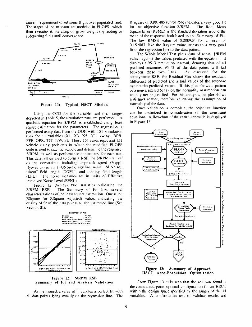
current requirement of subsonic flight over populated land.The stages of the mission are modeled in FLOPS, whichthen executes it, iterating on gross weight (by adding orsubtracting fuel) until convergence.

M = 2 a SM t_w_ n

CRUISE M _ o2'_tHI Iq

_O mm

ISLIMB

ABORT

/'i II_l_w r F = tg_> l= _t $1) t_ Si

SD ,_c;t

'_onm - _bn _,_ 14W_n m 24,'9 n m

q P'

Figure 11: Typical HSCT Mission

Using the CCD for the variables and their rangesdepicted in Table 5, the simulation runs are performed. Aquadratic equation for $/RPM is established using leastsquare estimators for the parameters. The regression isperformed using data from the DOE with 151 simulationruns for 11 variables (XI, X3, X5, YI, xwing, BPR,FPR. OPR, TIT, T/W, S). These 151 cases represent 151vehicle sizing problems in which the modified FLOPScode is used to size the vehicle and determine the response,$/RPM, as well as performance constraints, for each run.This data is then used to form a RSE for $/RPM as well

as the constraints, including approach speed (Vapp),flyover noise in (FONoise), sideline noise (SLNoise),takeoff field length (TOFL), and landing field length(LFL). The noise measures are in units of EffectivePerceived Noise Level (EPNL).

Figure 12 displays two statistics validating the$/RPM RSE. The Summary of Fit lists severalcharacterizations of the least square estimation. One is theRSquare (or RSquare Adjusted) value, indicating thequality of fit of the data points to the estimated line (SeeSection III).

Summar._ of Fit

RSqu,ac _ t_ 1495RSqu_¢ Adl 0 9¢,1_5_

Rt_a¢ Jt.lea, n Square Efft_¢ D IWX_5¢,

Mea_ ol Rcst_n,e (_ 152/_X7

Ob,_:_ _uon s i o[ SUlrl '_. gt _, I"l

() (X)I

• • • m . •

0 (W)I

-(IqWW)

. .'..1.

_+_w_ " "."::.._: :. ":

1,,_ " '.'.:Y """ •

-(I (W)I :, •, o.

I . | . I • i • I , !

fll_)l}l.15( 150{ 1521 1oi I 1_5

PM _t+,ll, h', I

$/RPM RSEFigure 12:Summary of Fit and Analysis Validation

As mentioned, a value of I denotes a perfect fit withall data points lying exactly on the regression line. The

R-square of 0.981485 (0.961956) indicates a very good fitfor the objective function $/RPM. The Root MeanSquare Error (RSME) is the standard deviation around themean of the response, both listed in the Summary of Fit.The low RMSE value of 0.000956 for a mean of

0.152887, like the Rsquare value, attests to a very goodfit of the regression line to the data points.

The Whole Model Test plots data of actual $/RPMvalues against the values predicted with the equation. Itdisplays a 95 _ prediction interval, denoting that of all

predicted outcomes, 95 % of the data points will fallbetween these two lines. As discussed for the

aerodynamic RSE, the Residual Plot shows the residuals(difference of predicted and actual value) of the responseagainst the predicted values. If this plot shows a patternor a non-scattered behavior, the normality assumption canusually not be justified. For this analysis, the plot showsa distinct scatter, therefore validating the assumption ofnormality of the data.

Once validation is complete, the objective functioncan be optimized in consideration of the constraintequations. A flowchart of the entire approach is displayedin Figure 13.

Clmfiguratbor, Dc,,wpl I,,_,

I &er_d_. nam_ RSE_

and ('_

j, I

No _tc_

, r

+Ctm_Uaa_'d JPoinl Dt'_l_n ( _r.llmurn

ln

g/RP_.I TIX.',_'r W R{)]-_, ¢1_ J

Rc_Txm_ Surla_c Fom_alh,r_ IB_x-Behnkcn I_IE

Map,

+.c

3

+z

Figure 13: Summary of ApproachHSCT Aero°Propulsion Optimization

From Figure 13, it is seen that the solution flmnd is

the constrained point optimal configuration for an HSCTwithin the design space specified by the ranges of the 11variables. A confirmation test to validate results and

9

obtain componentweightsis performed. Thesecomponent weights, together with the missionparameters, describe the optimal configuration which ispassed over to the Economic Viability Assessment, whereeconomic uncertainty is inu-oduced and the probability ofmeeting a target for the $/RPM is calculated.

The generation of both the aerodynamic RSEs as wellas the just inixoduced overall objective RSE for $/RPMwas accomplished via UNIX shell scripts, which managedthe process of setting up input files, running the specified

codes, in remote shells, and parsing output files for therequired response values. This process automation saved aconsiderable amount of time over a manual procedure ofrunning hundreds of simulations from the command line.

Results

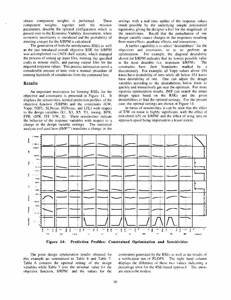
An important motivation for forming RSEs for theobjective and constraints is presented in Figure 14. Itdisplays the sensitivities, termed prediction profiles, of theobjective function ($/RPM) and the constraints (GW,Vapp, TOFL, SLNoise, FONoise, and LFL) with respectto the design variables (XI, X3, X5, YI, xwing, BPR,FPR, OPR, TIT, T/W, S). These sensitivities indicate

the behavior of the response variables with respect to achange in the design variable settings. The statisticalanalysis tool used here (JMP _]_) translates a change in the

settings with a real time update of the response values(made possible by the underlying simple polynomialequations), giving the designer a feel for the magnitude ofthe sensitivities. Recall that the perturbation of onedesign variable causes changes in the responses resultingfrom main effects, quadratic effects, and interactions.

A further capability is to select "desirabilities" for theobjectives and constraints so as to perform anoptimization. For example, the diagonal desirabilityshown for $/RPM indicates that its lowest possible valueis the most desirable (i.e. minimize $/RPM). Theconstraints have their boundaries marked by a

discontinuity. For example, all Vapp values above 154knots have desirability of zero while all below 154 knotshave desirability of one. One can adjust the designvariables according to the desirabilities below them toquickly and interactively get near the optimum. For morerigorous optimization results, JMP can search the entiredesign space based on the RSEs and the givendesirabilities to find the optimal settings. For the presentcase, the optimal settings are shown in Figure 14.

In terms of sensitivities, it can be seen that the effect

of T/W on noise is highly significant, with the effect ofroot chord (x5) on $/RPM and the effect of wing area onapproach speed being important to a lesser extent.

! i

Figure 14: Prediction Profiles: Constrained Optimization and Sensitivities

The point design optimization results obtained forthis example are summarized in Table 6 and Table 7.Table 6 contains the optimal setting of the designvariables while Table 7 lisls the minimal value l_r the

objective function, $/RPM, and the values for the

constraints generated by Ihc RSEs as well as the results ofa verification run of FLOPS. The right hand column

displays the difference of these tv, o values indicating apercentage error for the RSE-based approach The errorsare seen to be modest.

I0

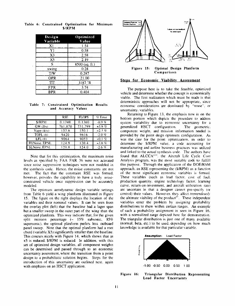
Table 6: Constrained Optimization for Minimum$/RPM

XI 1.54

Y1 0.58

X3 2.58

X5 2.19

xwingT/W

8500 (sq. ft.)

0.28

0.287

OPR 21.00

TIT 3187 °R

FPR 3.74

BPR 0.404

Table 7: Constrained Optimization Resultsand Accuracy Values

RSE

0.1348

Vapp (kts)TOFL (ft)

FLOPS

0.1360

c_ Error

-0.9 ch$/RPM

GW (lbs) 761,870 731,799 +3.9 ck

153.6 150.1 +2.3 %

9616

SLNoise, EPNL

9420 -2.0 ck

LFL tfl) 9064 9053 +0.1%FONoise, EPNL 124.9 120.4 +3.6 %

120.8 124.0 -2.6 c_

Note that for this optimization, the maximum noise

levels as specified by FAA FAR 36 were not activated

since noise suppression techniques were not modeled in

the synthesis code. Hence, the noise constraints are not

met. The fact that the constraint RSE was formed,

however, provides the capability to have a truly noise-

constrained vehicle once suppression can be accuratelymodeled.

The optimum aerodynamic design variable settings

from Table 6 yield a wing planform illustrated in Figure

15. The figure on the right displays the location of thevariables and their nominal values. It can be seen from

the overlay plot (left) that the baseline had a lager span

but a smaller sweep in the outer part of the wing than the

optimized planform. This may indicate that, for the given

split mission percentage (~ 15% subsonic, 85%

supersonic), the optimal planform prefers less outboard

panel sweep. Note that the optimal planform had a root

chord (variable X5) significantly smaller than the baseline.

This concurs nicely with Figure 14, which shows that as

x5 is reduced, $/RPM is reduced. In addition, with this

set of optimized design variables, all component weights

can be determined and passed through to an economic

uncertainty assessment, where the transition from a point

design to a probahilistic solution begins. Steps for the

introduction of this uncertainty are outlined next. again

with emphasis on an HSCT application.

x_,,

Figure 15: Optimal Design Planform

Comparison

Steps for Economic Viability Assessment

The purpose here is to take the feasible, optimized

vehicle and determine whether the concept is economically

viable. The first realization which must be made is that

deterministic approaches will not be appropriate, since

economic considerations are dominated by "noise", or

uncertainty, variables.

Returning to Figure 13, the emphasis now is on the

bottom portion which depicts the procedure to address

system variability due to economic uncertainty for a

generalized HSCT configuration. The geometric,

component weight, and mission information needed is

provided by the point deign optimum configuration. As

was the case for the point optimization, in order to

determine the $/RPM value, a code accounting for

manufacturing and airline business practices was utilized

and linked to the actual synthesis code. The authors have

found that ALCCA c_', the Aircraft Life Cy'cle Cost

Analysis program, was the most suitable code to fulfill

this purpose. Through the application of the DOE/RSM

approach, an RSE representing the ($/RPM) as a function

of the most significant economic variables is formed.

These variables (such as load factor, cost of fuel,

production quantity', engine technology factor, learning

curve, return-on-investment, and aircraft utilization rate)

are uncertain in thal a designer cannot pre-specil_ (or

control) their values. However. they' affect tremen&msh

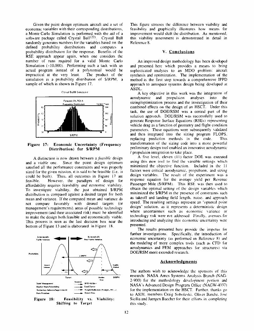
the ultimate viability of the product '_'. These independent

variables enter the problem by assigning probability'

distributions to them within certain ranges. An example

of such a probability assignment is seen in Figure 16,

with a normalized range depicted here for demonstration.

The triangular distribution is just one of many available

(normal, beta, etc.) to be used, depending on how much

knowledge is available for that particular variable.

Assumption: Load Factor

-1.00 -0.50 0.00 0.50 1.00

Figure 16: Triangular Distribution RepresentingLoad Factor Uncertainty

II

Given the point design optimum aircraft and a set ofeconomic variables with their corresponding distributions,a Monte Carlo Simulation is performed with the aid of asoftware package called Crystal Ball (22). Crystal Ballrandomly generates numbers for the variables based on thedefined probability distributions and computes aprobability distribution for the response. Benefits of theRSE approach appear again, when one considers thenumber of runs required for a valid Monte CarloSimulation (-10,000). Performing such a task with anactual program instead of a polynomial would beimpractical at the very least. The product of thesimulation is a probability distribution of $/RPM, asample of which is shown in Figure 17.

CD'stal Ball® Slmulattt,n

Forecast: 5% ROI-A

Frecl_enc Y Distributnon 101000 Trials

03 _ 334

O3 25O

D2 167

0_ 84

O0 0

S_q_,PM

Figure 17: Economic Uncertainty (FrequencyDistribution) for $/RPM

A distinction is now drawn between a feasible designand a viable one. Since the point design optimumsatisfied all the performance constraints and was properlysized for the given mission, it is said to be feasible (i.e. itcould be built). Thus. all outcomes in Figure 17 arefeasible. However. the paradigm of design foraffordabilily requires feasibility and economic viability.To investigate viability, the just obtained $/RPMdistribution is compared against a desired target for bothmean and variance. If the computed mean and variance donot compare favorably with desired targets (ormanagement's requirements), areas of possible technologyimprovement (and their associated risk) must be identifiedto make the design both feasible and economically viable.This process is seen as the last decision box near thebottom of Figure 13 and is elaborated in Figure 18.

b:t_mi¢ilt)

_, ialde _,oluth_ [l_ ['_c+morn knll_*Noo- _, iabl_ _ulkm

\ -Tar_el lu.-li,_ fdRpM

'd._r..,l

% ield M ilall_" me nl _ i(Ol I Airlin* )

MarkH _.bares'_:hed.l_nK _ L,_d l"ad,,r

Fare PT_mium _ Tkke! Prk_

Figure 18: Feasibility vs. Viability:Shifting to Target

This figure stresses the difference between viability andfeasibility and graphically illustrates how means forimprovement would shift the distribution. As mentioned,this viability assessment is demonstrated in detail inReference 8.

V. Conclusions

An improved design methodology has been developed

and presented here which provides a means to bringsophisticated analyses to an MDO problem: aircraftsynthesis and optimization. The implementation of themethod is the first step towards a comprehensive IPPDapproach to aerospace systems design being developed atASDL.

A key objective in this work was the integration ofaerodynamic and propulsion analyses into thesizing/optimization process and the investigation of theircombined effects on the design of an HSCT. Under thistask, the use of DOE/RSM was a central part of the

solution approach. DOE/RSM was successfully used togenerate Response Surface Equations (RSEs) representingvehicle drag as a function of geometry and flight conditionparameters. These equations were subsequently validatedand then integrated into the sizing program FLOPS.replacing prediction methods in the code. Thistransformation of the sizing code into a more powerfulpreliminary design tool enabled an innovative aerodynamic/ propulsion integration to take place.

A five level, eleven (11) factor DOE was executed

using this new tool to find the variable settings whichminimized the objective function. Included in the 11factors were critical aerodynamic, propulsion, and sizingdesign variables. The result of the experiment was aresponse equation for the average yield per RevenuePassenger Mile ($/RPM). This RSE was then used toobtain the optimal setting of the design variables whichminimized the $/RPM in the presence of constraints suchas takeoff and landing field length, noise, and approachspeed. The resulting settings represent an "optimal pointdesign" solution, as it represents a deterministic designwhere uncertainties such as economic variance or

technology risk were not addres_d. Finally, avenues forintroducing and analyzing this economic uncertainty werepresented.

The results presented here provide the impetus forfurther investigations. Specifically, the introduction ofeconomic uncertainty (as performed in Reference 8)the modeling of more complex tools (such as CFD for

aerodynamics and FEM approaches for structuresl viaDOE/RSM merit extended research.

Acknowledgments

The authors wish to acknowledge the sponsors of thisresearch: NASA Ames Systems Analysis Branch (NAG-2-900) for the methodology development portion and

NASA's Advanced Design Program Office (NAGW-4337)for the implementation on the HSCT. Further. thanks goto ASDL members Craig Soboleski, OIb, er Bandte, JoseSicilia and Juergen Baecher lot their cflorts in completingthis study.

12

Referencfs

I. Sobieszczanski-Sobieski, J., "MultidisciplinaryDesign Optimization: An Emerging New EngineeringDiscipline", The World Congress on Optimal Design ofStructural Systems, Rio de Janeiro, Brazil, August 1993.

2. Sobieszczanski-Sobieski, J., "A System Approachto Aircraft Optimization" AGARD Structures andMaterials Panel 72nd Meeting. Bath, United Kingdom,May, 199 I.

3. Dovi, Wren, Barthelemay, Coen."Multidisciplinary Design Integration System for aSupersonic Transport Aircraft", AGARD StructuresMaterials Panel 72ndMeeting, Bath, United Kingdom,May, 199 I.

4. Sobieszczanski-Sobieski, J. and Haftka, R.T.,

"'Multidisciplinary Aerospace Design Optimization:Survey of recent Developments", 34th Aerospace SciencesMeeting and Exhibit. Reno, NV, January 1995. AIAA96-0711.

5. Malone, B. and W. Mason, "MultidisciplinaryOptimization in Aircraft Design Using AnalyticTechnology Models". Journal of Aircraft, Vol. 32 No. 2,March-April 1995.

6. Giunta, A.A., Balabanov, V., Kaufman, M.,

Burgee, S., Grossman, B., Haftka, R.T.. Mason, W.H.,and Watson. L.T., "Variable-Complexity ResponseSurface Design of an HSCT Configuration." inProceedings of ICASE/LaRC Workshop onMultidisciplinary Design Optimization, Hampton, VA,March, 1995.

7. Engelund, W.C., Stanley, D.O., Lepsch, R.A.,McMillian, M.M., "Aerodynamic Configuration DesignUsing Response Surface methodology Analysis," AIAAAircraft Design, Systems, and Operations Meeting,Monterey, CA. 11- 13 August, 1993.

8. Mavris, D. N., Bandte, O., Schrage D.P.,"Economic Uncertainty Assessment of an HSCT using aCombined Design of Experiments / Monte Carlo

Approach," 17th Annual Conference of the ISPA, SanDiego. CA, May 1995.

9. McCullers, L.A. Flight Optimization SystemUser's Guide, Version 5.7, NASA Langley ResearchCenter, 1995.

10. Box, G.E.P., Draper, N.R., Empirical Model-

B0ilding and Response Surfaces, John Wiley & Sons,Inc., New York; 1987.

II. Box, G.E.P., Hunter, W.G.. Hunter, J.S..

Statistics for Experimenters, John Wiley & Sons, Inc..New York, 1978.

12. SAS Institute Inc., JMP Computer Program ce_User's Manual, Cary, NC, 1994.

13. Dieter, G.E., Engineering Design. A Materials

and Processing Approach, 2nd Edition, McGraw HillInc., New York, NY, 1971.

14. Montgomery, D.C., Design and Analysis of

Experiments, John Wiley & Sons, Inc., New York, 1991.

15. Swan, W. "Design Evolution of the Boeing 2707-300 Supersonic Transport". Boeing Commercial AirplaneCompany, No Date Available.

16. Sakata, I.F., and Davis, G.W., "Evaluation of

Structural Design Concepts for Arrow-Wing SupersonicCruise Aircraft," NASA CR-2667, May, 1977.

17. BDAP- Middleton. W.D., Lundry. J.L., "ASystem for Aerodynamic Design and Analysis ofSupersonic Aircraft," NASA-CR-3351, 1980.

18. "WINGDES", Carlson, HW., Walkley, K.B.,"Numerical Methods and a Computer Program forSubsonic and Supersonic Aerodynamic Design andAnalysis of Wings with Attainable ThrustConsiderations", NASA-CR-3803, 1984.

19. Carlson, H.W., Darden, C.M., Mann, M.J.,

"Validation of a Computer Code for Analysis of SubsonicAerodynamic Performance of Wings with Flaps inCombination with a Canard or Horizontal Tail and a

Application to Optimization," (AERO2S), NASA-TP-2961, 1990.

20. "AWAVE User's Guide tor the Revised Wave

Drag Analysis Program, NASA Langley Research Center.September, 1992.

21. Galloway, T.L., and Mavris. D.N., Aircrqfi L(I_'Cycle Cost Analysis (ALCCA) Program, NASA AmesResearch Center. September 1993.

22. Decisioneering, Inc., Crwstal Ball. ComputerProgram and Users Guide, Denver, CO, 1993.

13