NOTES ON INTRODUCTORY COMBINATORICS

bY

Donald R. Woods

STAN-CS-79-732April 1979

COMPUTER SCIENCE DEPARTMENTSchool of Humanities and Sciences

STANFORD UNIVERSITY

N o t e s OH Introductory Cam bhatorics

DollaId R. Woods

Computer Science DepartmentStauford University

Stanford, Califomia 94305

Abstract

In the spring of 1978, Professors George P6lya and Robert Tarjan teamed up to teach CS1504ntroduction to Combinatorics. This report consists primarily of the class notes and otherhandouts produced by the author as teaching assistant for the course.

Among the topics covered are elementary subjects such as combinations and permutations,mathematical tools such as generating functions and P6lya’s Theory of Counting, and analyses ofspecific problems such as Ramsey Theory, matchings, and Hamiltonian and Eulerian paths.

Publication of these notes was supported by a grant from IBM Corporation.

Table of Contents

1. Introduction . . . . . . . . . . . . . . . . . . . . . . . . . . . . . . 1

2. Combinations and Permutations . . . . . . . . . . . . . . . . . . . . . . . 1

3. Generating Functions . . . . . . . . . . . . . . . . . . . . . . . . . . . 7

4. Principle of Inclusion and Exclusion . . . . . . . . . . . . . . . . . . . . . 21

5. St i r l ing Numbers . . . . . . . . . . . . . . . . . . . . . . . . . . . . . 2 6

6. P6lya’s Theory of Count ing . . . . . . . . . . . . . . . . . . . . . . . . . 34

7 . O u t l o o k -54. . >r- . . . . . . . . . . . . . . . . . . . . . . . . . . . .

8 . Midterm Examinat ion . . . . . . . . . . . . . . . . . . . . . . . . . . . 59

9. Ramsey Theory . . . . . . . . . . . . . . . . . . . . . . . . . . . . . 72

10.

Il.

12.

- 13.

14.

15.

16.

Matchings (Stable Marriages) . . . . . . . . . . . . . . . . . . . . . . . . 79

Matchings (Maximum Matchings) . . . . . . . . . . . . . . . . . . . . . . 8 3

Network Flow . . . . . . . . . . . . . . . . . . . . . . . . . . . . . 94

Hamiltonian and Eulerian Paths . . . . . . . . . . . . . . . . . . . . . . 9 7

Planarity and the Four-Color Theorem . . . . . . . . . . . . . . . . . . . 104

Final Examination . . . . . . . . . . . . . . . . . . . . . . . . . . . 112

Bibl iography . . . . . . . . . . . . . . . . . . . . . . . . . . . . . 117

Introduction

For the most part the notes that comprise this report differ only slightly from those provided to thestudents during the course. The notes have been merged into a single paper, a few sections havebeen made more detailed, and various corrigenda have been incorporated. The midterm and finalexaminations are included in their proper chronological places within the text (sections 8 and 15),together with the solutions. The only information omitted from this report is that regarding themechanics of the course-office hours, grading criteria, etc. Homework assignments are included, asthey often led to further discussion in the notes. Lecture dates are included to give a feel for thepace at which material was covered, though it should be noted that much of the material in thenotes was not actually presented in the lectures, being instead drawn from notes provided by theinstructors or supplied by the author as the notes were written.

A brief word of explanation regarding the dual instructorship of the course: Professor P6lyataught the first two-thirds of the course, reflected in sections 2 through ‘I of this report. ProfessorTarjan taught the remainder of the course, as covered in sections 9 through 14.

Though there was no formal text for CS 150, a number of books were made available forreference. These books, along with additional texts used by the author in preparing the notes, arelisted in the bibliography at the end of this report. The [bracketed] abbreviations given there willbe used when referring to one of Polya’s books; the other texts will be referred to by their authors.Though all of the books contain relevant material, not all are specifically referenced in the notes. Inparticular, all mentions of [Harary] refer to Graph Theory and not to A Seminar on Graph Theory.

The author would like to thank Christopher J. Van Wyk for supplying excellent proofreadingassistance, Donald E. Knuth for finding the funds to support publication of the notes and, of course,Professors PcSlya and Tarjan for providing ample source material.

q2 Combinations and Permutations

January 5. This was an introductory lecture in which P6lya discussed in general terms just whatcombinatorics is about: The study of counting various combinations or configurations. He startedwith a problem based on the mystical sign known, appropriately, as an “abracadabra”.

eA

RBRBRA A A A

c c c c cADADAOADADA

ABABABAR R

A

The question is, how many different ways are there to spell out “abracadabra”, always going fromone letter to an adjacent letter? Due to the way some letters (especially C and D) are found only incertain rows, it turns out the only ways to spell “abracadabra” start with the topmost ‘A’ and zig-zagdown to the bottommost ‘A’. If we think of the letters as points, then any spelling of “abracadabra”specifies a sequence of points forming a crooked line from the top to the bottom. One such line isshown on the following page.

- 2 -

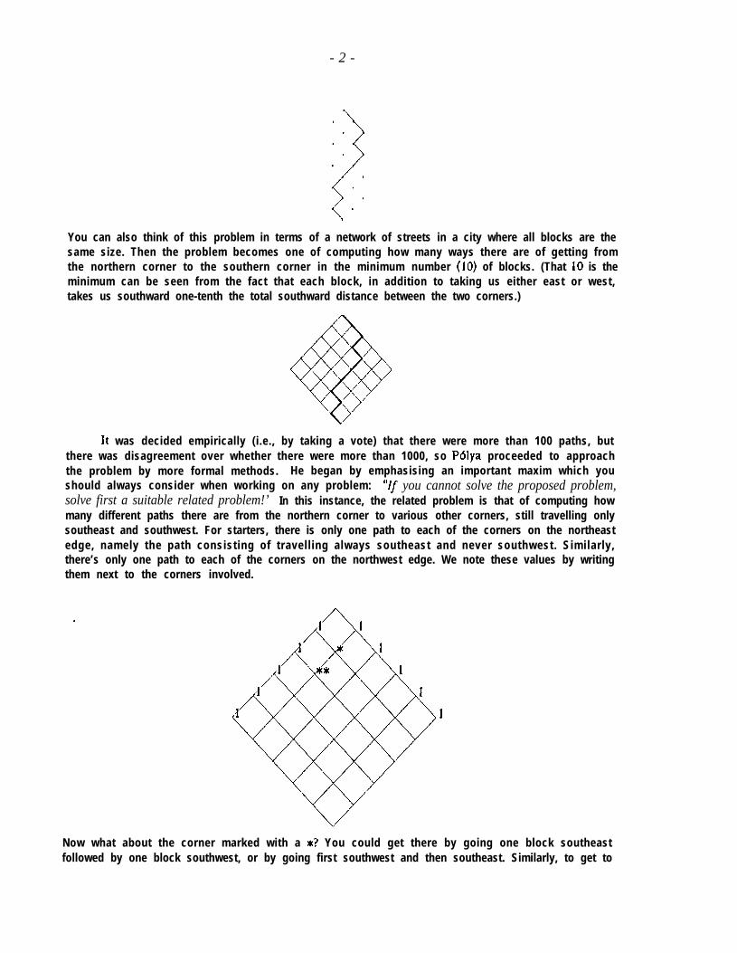
You can also think of this problem in terms of a network of streets in a city where all blocks are thesame size. Then the problem becomes one of computing how many ways there are of getting fromthe northern corner to the southern corner in the minimum number (IO) of blocks. (That 10 is theminimum can be seen from the fact that each block, in addition to taking us either east or west,takes us southward one-tenth the total southward distance between the two corners.)

It was decided empirically (i.e., by taking a vote) that there were more than 100 paths, butthere was disagreement over whether there were more than 1000, so P6lya proceeded to approachthe problem by more formal methods. He began by emphasising an important maxim which youshould always consider when working on any problem:solve first a suitable related problem!’

“If you cannot solve the proposed problem,In this instance, the related problem is that of computing how

many different paths there are from the northern corner to various other corners, still travelling onlysoutheast and southwest. For starters, there is only one path to each of the corners on the northeastedge, namely the path consisting of travelling always southeast and never southwest. Similarly,there’s only one path to each of the corners on the northwest edge. We note these values by writingthem next to the corners involved.

Now what about the corner marked with a *? You could get there by going one block southeastfollowed by one block southwest, or by going first southwest and then southeast. Similarly, to get to

-3-

the corner marked x*, you could go southeast, then southwest twice, or you could go southwest, thensoutheast, then southwest, or you could go southwest twice and then southeast. Moving down thediagonal this way, and (by symmetry) the corresponding diagonal on the eastern side, we can fili insome more values.

1

Had we tried to go much further like this, it would probably have gotten tiresome, so insteadwe came up with a general observation regarding an arbitrary corner, such as the one marked zabove. If we know that there are x ways to get to the corner just northwest of z, and y ways to getto the corner northeast of z, then there are xty ways to get to z, since to get there we must first get toeither x or y, after which there’s only one way to continue on to z. For instance, there are 3+3=6paths to the corner marked rlc. This general rule provides us with an easy way to finish computingthe number of paths to the southern corner. The first homework assignment was to complete thiscomputation. Not surprisingly, everyone got it right. For the record, here it is.

The numbers we’ve been computing are known as binomial coefficients, for reasons we’ll getto eventually. The arrangement of numbers, when cut off by any horizontal line so as to form atriangular pattern, is known as Pascal’s trianqie. (Pascal referred to it as “the arithmetical triangle”.)The numbers are uniquely defined by the boundary condition (the I’s along the edges) together withthe recursion formula (each number not on the edge is the sum of the two above it). In addition tothis recursion formula, which defines each number in terms of earlier ones, there is another way tolook at the situation. Here’s a small chunk of the street network we’ve been working with:

-4-

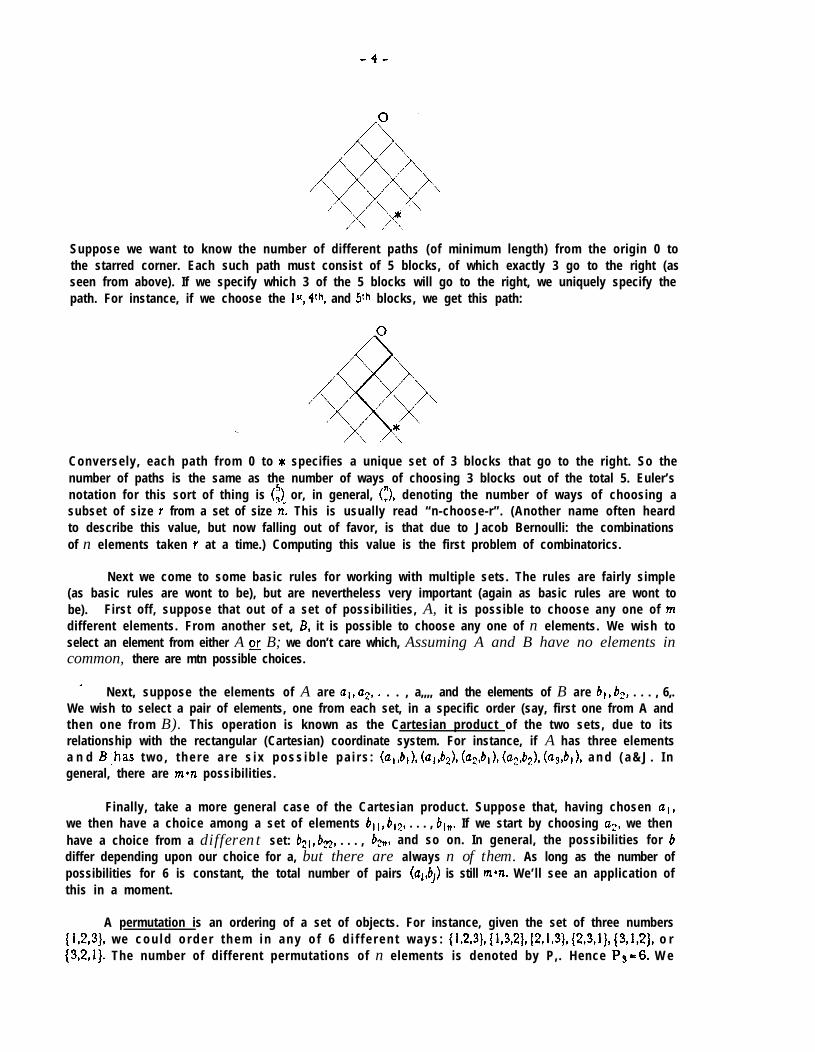
Suppose we want to know the number of different paths (of minimum length) from the origin 0 tothe starred corner. Each such path must consist of 5 blocks, of which exactly 3 go to the right (asseen from above). If we specify which 3 of the 5 blocks will go to the right, we uniquely specify thepath. For instance, if we choose the I&t, Qth, and 5th blocks, we get this path:

Conversely, each path from 0 to * specifies a unique set of 3 blocks that go to the right. So thenumber of paths is the same as the number of ways of choosing 3 blocks out of the total 5. Euler’snotation for this sort of thing is (4, or, in general, (r), denoting the number of ways of choosing asubset of size r from a set of size n’. This is usually read “n-choose-r”. (Another name often heardto describe this value, but now falling out of favor, is that due to Jacob Bernoulli: the combinationsof n elements taken Y at a time.) Computing this value is the first problem of combinatorics.

Next we come to some basic rules for working with multiple sets. The rules are fairly simple(as basic rules are wont to be), but are nevertheless very important (again as basic rules are wont tobe). First off, suppose that out of a set of possibilities, A, it is possible to choose any one of mdifferent elements. From another set, B, it is possible to choose any one of n elements. We wish toselect an element from either A or B; we don’t care which, Assuming A and B have no elements incommon, there are mtn possible choices.

-Next, suppose the elements of A are al, a2,. . . , a,,,, and the elements of B are b,, b2, . . . , 6,.

We wish to select a pair of elements, one from each set, in a specific order (say, first one from A andthen one from B). This operation is known as the Cartesian product of the two sets, due to itsrelationship with the rectangular (Cartesian) coordinate system. For instance, if A has three elementsa n d B -has t w o , t h e r e a r e s i x p o s s i b l e p a i r s : (a,,bJ (a&), (up,bI), (aZ,bZ), (~,b,), a n d ( a & J . I ngeneral, there are men possibilities.

Finally, take a more general case of the Cartesian product. Suppose that, having chosen aI,we then have a choice among a set of elements 6, ,, b12, . . . , b,,. If we start by choosing a2, we thenhave a choice from a different set: bZI, bZ2, . . . , b:,, and so on. In general, the possibilities for bdiffer depending upon our choice for a, but there are always n of them. As long as the number ofpossibilities for 6 is constant, the total number of pairs (al,6,) is still men. We’ll see an application ofthis in a moment.

A permutation is an ordering of a set of objects. For instance, given the set of three numbers(1,2,3}, w e c o u l d o r d e r t h e m i n a n y o f 6 d i f f e r e n t w a y s : {1,2,3), (1,3,2), (2,1,3), (2,3,1), (3,&Z], o r(3,2,1]. The number of different permutations of n elements is denoted by P,. Hence P3 - 6. W e

-5-

a l s o s e e f a i r l y e a s i l y t h a t Pi = I a n d Pz = 2. At this point Polya brought up another impor tantmaxim: “The beginning of most discoveries is to recognise a pattern.” There is a pattern to the threenumbers we’ve got so far; to make it more apparent, we can rewrite them as follows:

P,=l=lP? - 2s I@2Ps=6= 1*2*3* .

We conjecture that P, = I l 2 l 3 l . . . l n. This product is called n factorial and is usually writtentt (99

p:+;Now we need to prove our conjecture. Well, suppose it’s true that P, = n!. Then what would

be? It is the number of ways of ordering nt 1 objects. The ntP object could be in any one ofn+ 1 positions. Whichever position we choose for it, the remaining n objects can be ordered in anyof P, ways. Using the generaiisation of the Cartesian product rule, we conclude that the totalnumber o f ways we can order n+i objects is (nt l)*P,. Therefore, if P, = I l 2 l 3 l . . . l n, thenP n+l = 1 l 2*3*... l n l (n+ I) = (n+i)!. But we know that P9 = 3!, so taking n=3 we conclude thatP4 = 4!. Knowing this, we can take n-4 and conclude that P5 = 5!, and so on. For any finite n, wecan prove that P, = n! by starting at PI\ and chugging away for a while. This method of proof,which Polya describes as “a diabolic way of proving things”, is called mathematical induction. It isextremely useful since it saves you from having to figure out the formula you’re proving. If you canmake a “lucky guess” as to what the answer is, you may be able to prove it by induction.

January 10. Polya began the lecture by reviewing the material from the previous lecture. In doingso he brought out some points that hadn’t been explicitly stated before. First, there’s the formaldefinition of the binomial coefficients:

B o u n d a r y c o n d i t i o n : (:) = (,“) - 1

Recursion: c:‘, = (.n,) + q. [n and Y integers, O<r<nt 11

Similarly, P, can be defined by boundary conditions and recursion:

B o u n d a r y c o n d i t i o n : P i - l! = 1

Recursion: P, = n! = nP,,i.

If we apply this recursion formula with n=i, we find that Pi = l*PO. Hence we define PO = O! = 1.-

From here, we move on to look at something called a “variation”, a word you may immediatelyforget. It is defined as follows. Given a set of n objects, we wish to choose Y of them in some order.That is, choosing the first object and then the second would be considered different from choosingthe second and then the first. How many such variations are there? One approach is to start by

* choosing some object to be the first one selected. There are n choices. For each choice, there aren-l choices for the second object. Thus, by the product rule, there are n(n-I) choices for the firsttwo objects together. For each such pair, there are (n-2) objects remaining from which to choose thethird object. So there are n(n-l)(n-2) choices for the first three objects. Continuing in this manner,we find that there are n(n- l)(n-2) . . . (n-r+ I) variations.

We can often learn something by solving a problem in two different ways, so here’s a secondapproach. We first choose the subset of Y objects from among the n, We know there are (:) ways todo this. We then choose the ordering for the t objects. We know how many ways there are to dothis, too; it’s P,. So there are (:)*P, variations. But this answer must be the same as the one we gotthe other way. Therefore (:)*P, = n(n-l)(n-2). . . (n-rtl). Thus we learn something new:

- 6 -

( n ) p n(n-l)(n-2) . . . (n-r+ 1)r

Y!

= n(n- l)(n-2) . . . (n-r+ 1)14*3v..*r ’

(Note that, in the second form, the sum of ‘corresponding’ terms in the numerator and denominatoris always n+ 1; this is a useful mnemonic for remembering what the last term in the numerator is.)For example, the number that we computed for the first homework assignment is (‘,3, which is(10*9*8*7*6)/( I l 2*3*4*5) = (10*9*7*6)/( 1*3*5) = (2*9*7*6)/3 = 2*9*7*2 = 252. It’s always a good idea totest out a formula on some special cases where we already know the answer, so let’s look at (,“) and(i). W e h a v e

(n) e: n(n-l)(n-2) . . . 1n lC+3~..d

which, since the numerator and denominator have all the same factors, albeit in different orders,indeed equals 1. (i), however, poses a bit of a problem, since the numerator has no factors. Bydefining the product of zero factors to be equal to 1 (just as O! = I) we find that (i) - I as expected.

Another way to get this explicit form for the binomial coefficients is by using mathematicalinduction. We assume it’s true for small n (we can check this by hand) and then show that, if it’strue for n, it’s true for nt 1. The first problem on the second homework assignment was to carry outthis proof. Here it is: We assume that, for some value of n,

(n) = n(n- l)(n-2) . . . (n-w 11r 1 *2*3*,./r

for all values of t. Substituting r-l for I, we find

( 7t ) ID n(n-1X72-2) . . e (n-r+21r-l 1 l 2 * 3 l . . . l (r-l) *

By the definition of the binomial coefficients, we know that

t”:‘, = (,“J + t:,= n(n-l)(n-2) . . . (n-rt2) + n(n-l)(n-2) . . . (n-r+ 1)

1 l 2 l 3 l . . . ’ (r-l) 1*2*3v..*r

= n(n-i)(n-2) . . . (n-rt2) l r + n(n-l)(n-2) . .I . (n-r+ I)I l 2*3*...+-l)*r I l 2,3*...*r

= n(n-l)(n-2) . . . (n-M) l (Y t n-7+ 1)I l 2 ’ 3 l . . . l (Y-l) l Y

L: (n+ l)n(n-l)(n-2) . . . (n-rt2)I *2*3*,./r ’

which is the formula we’re trying to prove (with nt 1 substituted for n). Hence, if the formula istrue for n, it’s true for nt 1. This, combined with the fact that it’s true for n=l, means it is true forall finite n. (Actually, there’s a minor flaw in this proof. To wit, the recursion formula cannot beused to compute (L) or (:), since it would involve coefficients outside the range 0 < Y 5 n. However ,we’ve already shown separately that these two special cases satisfy the formula, so we’re all right.)

A more compact way to write the formula for the binomial coefficient can be derived bymultiplying both the numerator and denominator by the factors (n-r), (n-r-l), and so on down to 1.

-7.

(n) = n(n- l)(n-2) . . . (n-r+ 1) * (n-r)(n-r-l) . . . 2 e 1r (1 Q~3~..*r)(l 4*...4n-r-l)*((n-r))

=-IL-r!(n-r)!

Notice that, by this formula, it is immediately apparent that (:) = (,,rr). This was to be expected,since by the method of its construction Pascal’s triangle Is clearly symmetric.

Next, we consider n houses. They are built identically, because it’s easier that way. But then,to make them look different, they are painted different colors: Y of them are painted red, s of themyellow, and the remaining t of them green. In how many ways can we assign the colors to thehouses? We first choose which houses will be painted red; there are <:) ways to make this choice.Whatever choice we make, there are n-r houses left, of which we choose s to be painted yellow; thereare (“,-‘) ways to do this. At this point we have no choices left to make, since all the rest must begreen (that is, rts+t=n). So what do we have? By the product rule, there are (:,(“;‘) ways to paintthe houses, Using the formula we worked out a moment ago, we find

(;)(n;‘) = n! . (n-r)!r!( n-r)! s!( n-r-s)! l

But n-r-s-t, and the (n-r)! factors cancel, leaving us with

n!

which is, fortunately, symmetric with respect to Y, s, and t. (The alternative to its being symmetricwould be for it to be wrong, since the original problem was symmetric.) This sort of formula iscalled a multinomial coefficient.

rl3 Generating Functions

Generating functions are a general mathematical tool developed by de Moivre, Stirling, and Euler inthe 18th century, and are used often in combinatorics. As usual, we start with a concrete example:In how many ways can you change a dollar? We’ll assume we’re dealing with only five types of

- coins-pennies, nickels, dimes, quarters, and half dollars.

We first consider how many pennies to use. We could use one, or two, or three, etc., and ofcourse we could use none. We can show these choices pictorially:

Similarly, we have an infinite number of choices as to how many nickels we use (although for almostall such choices we’ll have more than a dollar already), and how many dimes, and so on:

-8-

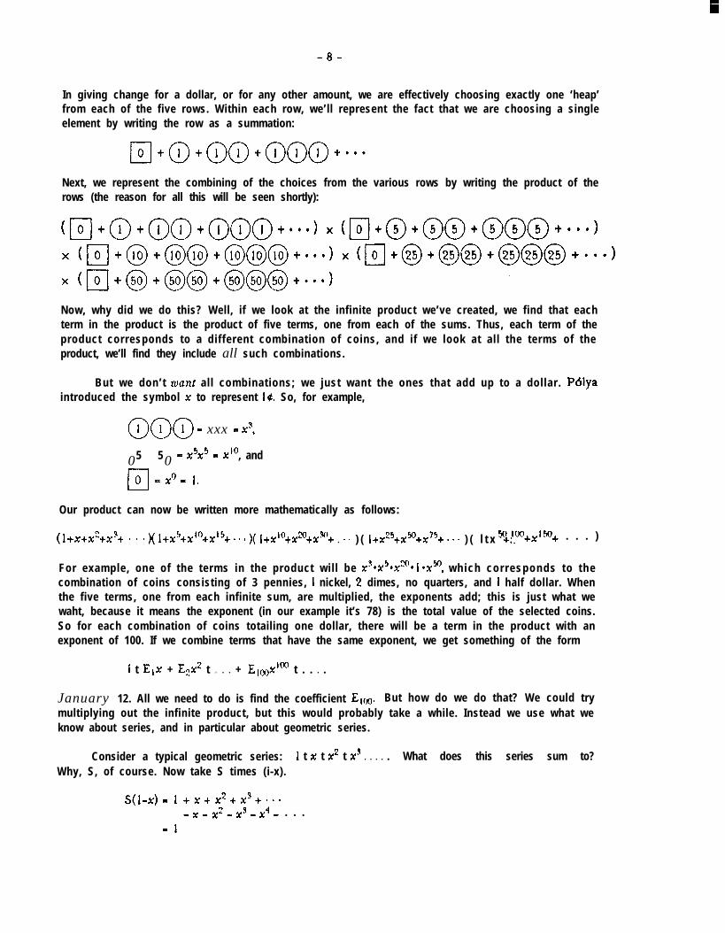
In giving change for a dollar, or for any other amount, we are effectively choosing exactly one ‘heap’from each of the five rows. Within each row, we’ll represent the fact that we are choosing a singleelement by writing the row as a summation:

Next, we represent the combining of the choices from the various rows by writing the product of therows (the reason for all this will be seen shortly):

Now, why did we do this? Well, if we look at the infinite product we’ve created, we find that eachterm in the product is the product of five terms, one from each of the sums. Thus, each term of theproduct corresponds to a different combination of coins, and if we look at all the terms of theproduct, we’ll find they include all such combinations.

But we don’t want all combinations; we just want the ones that add up to a dollar. Pblyaintroduced the symbol x to represent I#. So, for example,

@(i-J@ = xxx = 2,

0 05 5 0 x5x5 E X’O, and

Our product can now be written more mathematically as follows:

(l+xtx”tx”+ ’ ’ ’ )( ltx5tx’otx’5t ’ ’ ’ )( 1+x’“+x~tx% l ’ ’ ) ( ltX2%X%X’5t * * * ) ( l t x .+xfJf-’ ‘fJQp+ . . . )

For example, one of the terms in the product will be x3*x5~x~‘* l*xcn, which corresponds to thecombination of coins consisting of 3 pennies, I nickel, 2 dimes, no quarters, and 1 half dollar. Whenthe five terms, one from each infinite sum, are multiplied, the exponents add; this is just what wewaht, because it means the exponent (in our example it’s 78) is the total value of the selected coins.So for each combination of coins totailing one dollar, there will be a term in the product with anexponent of 100. If we combine terms that have the same exponent, we get something of the form

1 t E,x + Ezx2 t . l l + EiOOxlM t . . l .

January 12. All we need to do is find the coefficient Elm. But how do we do that? We could trymultiplying out the infinite product, but this would probably take a while. Instead we use what weknow about series, and in particular about geometric series.

Consider a typical geometric series: 1 t x t x2 t x3 t l l l . What does this series sum to?Why, S, of course. Now take S times (i-x).

S(l-x)= 1 txtx2tx3t'**- x - x2 - x3 - f' - . . .

= 1

S o S = 1/(1-x). S i m i l a r l y , 1 t x5 t x” t x I5 t ’ + 9 = I/( l-x”). Our infinite product thus simplifies tothe somewhat more compact form

I( l -x) ( i-x5)( i-x”‘){ I-x”)( l-xW) ’

which we can turn back into a series in powers of x, even though we don’t yet know the coefficientsn u m e r i c a l l y , a s

ii E,x”.n-0

Such a summation, in either form, is called the generating function for the sequence Eo, El, EZ, . . . .

So far so good, but we don’t seem to be any closer to computing Eloo than we were before.Once again we’ll try first solving an easier related problem. In fact, we’ll set up a sequence ofproblems leading to the one we’re interested in.

1( l - x ) ( l - x ” ) = jio Bnxn

1( l - x ) ( l-x5)( 1-p) = :. cnxn

I( l - x ) ( l-x5)( l-x’“){ l-x2’) = :o DnXn

We a l ready know that A , = 1 for all n L 0. What about Bn? We take the secondand multiply both sides by l-x5. The left side becomes 1/(1-x), which is series A.

-

$ Anxnn=O

= (l-x5)(: Bnxn)n-0

= (F(, Bnx”) - ( 2 B,x”+~)n=O

equation above

What does it mean for these two sums to be equal? Since they must be equal for all values of x, itmeans that the coefficients of x” must be equal for all n. On the left side the coefficient is simplyAn- On the right side, the first summation contributes a term of Bnxn’ and the second summationcontributes -B n-5x” (coming from multiplying (-x5) by Bn-5xn-5). Therefore

An = Bn - Bn-5

or, rearranging things,

Bn = An + Bn-5*

- io-

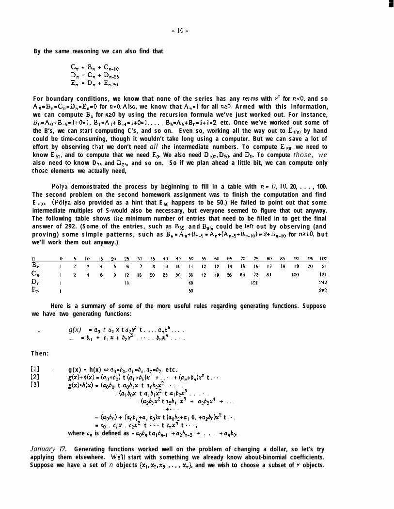
By the same reasoning we can also find that

cn = Bn + %I0

Dn r cn + Dn-25

En = Dn + En-w-

For boundary conditions, we know that none of the series has any terms with x” for n<O, and soAn=Bn=Cn=Dn=En=O for n<O. Also, we know that An=1 for all nr0. Armed wi th th is in format ion,we can compute B, for nr0 by using the recursion formula we’ve just worked out. For instance,+A (,+EL5= ltO=l, B,=A,tB,.,=itO=l,..., B5=A5tBO=ltl=2, etc. Once we’ve worked out some ofthe B’s, we can seat-t computing C’s, and so on. Even so, working all the way out to Eloo by handcould be time-consuming, though it wouldn’t take long using a computer. But we can save a lot ofeffort by observing that we don’t need all the intermediate numbers. To compute Elm we need toknow En, and to compute that we need Eo. We also need Dloo, Dw, and Do. To compute those, wealso need to know D f5 and Dz5, and so on. So if we plan ahead a little bit, we can compute onlythose elements we actually need,

P6iya demonstrated the process by beginning to fill in a table with n = 0, IO, 20, . . . , 100.The second problem on the second homework assignment was to finish the computation and findE Im. (Pdiya also provided as a hint that E 5. happens to be 50.) He failed to point out that someintermediate multiples of S-would also be necessary, but everyone seemed to figure that out anyway.The following table shows the minimum number of entries that need to be filled in to get the finalanswer of 292. (Some of the entries, such as BB5 a n d Bg5, could be left out by observ ing (andp r o v i n g ) s o m e s i m p l e p a t t e r n s , s u c h a s Bn = AntBn-5 = Ant(A+5tBn-,O) = 2tBn-,0 for m10, b u twe’ll work them out anyway.)

n 0 5 IO 15 20 25 30 35 40 45 50 55 60 65 70 75 80 85 90 95 100

Bn I 2 3 4 5 6 7 8 9 IO II 12 I3 ‘4 ‘5 I6 ‘7 ‘8 19 20 21

cn I 2 4 6 9 12 I6 20 25 flo 36 42 49 56 64 f2 81 I@0 ‘2’

Dn I I3 49 I21 242En I 50 292

Here is a summary of some of the more useful rules regarding generating functions. Supposewe have two generating functions:

g(x) = a0 t al x t a2x2 t . l l t a,x” t l . l

h(X) = 60 + 6, x t 62~’ + * * l t 6,X" t l * l

T h e n :

g ( x ) = h (x) e ao=:bo, al =b,, a2=b2, e t c .g(X)+h(X) = (aotbo) t (ul+bl)X t l l * t (Gntbn)x’ t l s 0g(x)+(x) = (aobo t ao6,x t aob2x2 t s l a )

t (albox t u,6,x2 t qbzxJ t l . + )

t (~~260~ t u:bl x3 t ~262~~ t l l l )

+ * . .

= (Qo) + (@I +a, 6,4x t (aob2tu, 6, tu2bo)x2 t l 9 l

= co t C�X t +x2 t ’ ’ ’ t CnXR t * ’ * ’where Cn is defined as = aObn t Ulbn,) t Q26n-2 t . . . t anbo.

January 17. Generating functions worked well on the problem of changing a dollar, so let’s tryapplying them elsewhere. We’ll start with something we already know about-binomial coefficients.Suppose we have a set of n objects (xl, x2, x3, , . , , x,), and we wish co choose a subset of Y objects.

- 11 -

We either choose xi or we don’t. As before, we’ll represent this choice by a sum of the possibilities,(xIo+xi ‘), or s imply (1+x,). S imi lar ly we have (I+x~), (1+x&, and SO o n . W e a g a i n r e p r e s e n t t h ecombination of choices by a product:

(1+x,)( 1+x2)( 1+x9) . . . (1+x,).

Each term of this product constitutes a selection of exactly one term from each of the n s u m s ,corresponding to a selection of some number (not necessarily Y) of objects from the original set. Forinstance, if we choose the xi from the first sum and the I from each of the others, we get the terma~. The product comes out to

1 + XI + x2 + XQ + ' ' ' + x,

+ XIX2 + XlXQ t x2x3 t � l t ⌧,,p,

t Xpt23cQ t xp~xq t ' * ' t x,,2x,,p,

t #&+3 * . . x,.

The number of ways of choosing, say, two x’s is the number of terms that contain exactly two x’s.So le t a l l the x1 be equal ; that is , le t xl = 3c2 = x3 - l s a = x, - x. T h e n

(1+x,)( 1+x2)( 1-q). . , (Itx,) = ( ItX)n = a0 + up t up2 + ’ ’ ’ t a#.

a0 is clearly 1; what about a,? It is equal to the number of terms in the product that contain exactlyo n e X, which is therefore the number of d i f ferent subsets of s ize 1. H e n c e al = (y). S i m i l a r l y ,a2 = the number of different subsets of size 2 = (i), and so on. For that matter, a0 = 1 - (i). We cansummarise all this in one handy equation:

n( ltX)n = c <y.

k=O

This is called the “binomial formula” (because Itx is the “basic” polynomial of two terms); hence thename “binomial coefficients”.

Polya next brought up a third maxim: “If you have a general formulu, try it out on somespecial cases,” One special case is x - 1. This gives us-

2” = $9 + <�I�, + (;I + � l � + q,

which is the number of subsets of all sizes from a set of size n. This checks, since for each objectwe have two choices-either it is in the subset or it isn’t. We have n such choices, and by the

. product rule the total number of possibilities is therefore the product of n 2’s.

Another interesting special case, which didn’t come up in the lecture, is that of x - -1:

on = (g) - (Y) t Q - * ’ ’ t (-I)“(;).

That this sum should be zero is obvious when n is odd, due to the symmetry of Pascal’s triangle.When n is even, however, the above result is less obvious, so this identity is worth noting. Note inparticular that, substituting the value n=O, we can deduce 0’ must equal 1.

Next, let’s consider the combinations of n objects with repetition taken t at a time, which we’lldenote by R,(‘? We can also think of it as having n kinds of objects, with an unlimited supply of

- l2-

each, from which we wish to select Y objects. Let’s find the generating function for this.

Just as when we were looking at ways to break a dollar, we can have no xi’s, or one XI, ortwo, or three, etc., and we’ll write this as the sum It#,t#I#It#I#I#~t 0 . . , and similarly for each x inthe set. We take the product,

(lt#~t#~#~t#~#~#~t ” ‘) l (l+#2+#2#2+#2#2#2+ get ’ ) l * *. ’ (l+#~t#~#~t#~#~#~+ ” ’ ),

so that, as usual, each term of the product corresponds to one of the possible selections. W e ’ r einterested in the selections that include exactly Y x’s (not necessarily different x’s), and we don’t wantto distinguish among the x’s, so we let xl = x2 - 0 l l - x, - #, and get

(lt#t#‘t#~t * * * )“.

Each term that selects exactly Y x’s contributes 1 to the coefficient of #‘, so that’s the coefficient wewant. Well, we know what the geometric series sums to, so what we’ve got is

Let us digress for a moment and examine a useful generalisation of binomial coefficients.Newton defined (T) for non-integer oc as

(“) = c&c-l)(oc-2) . . * (c7xt 1)r 14?*3*...*r

and claimed that, if Ixlcl,

b)(1+x)” = c Q#”

k-0

for all CL Newton didn’t actually prove this (rigorous proofs were not recognised as being necessaryin his day), but Gauss proved it in 1812. We won’ t bother to show the proof here . Using th isresult, we find

( l - x ) ‘ ” = iit (-,“,W.k=O

Since R$“) is the coefficient of x’ in this sum, we find

Rp) = (-r’)*(-l)r

p (-n)(-n-1)(-n-2) . . . (-n-Y+ 1) (-1)’1 l 2*3*...*r ’

Combining the Y factors of -1 with the Y terms in the numerator, we get

R(n) - n(nt l)(ntt?) . . . (ntr-i)r 1 l 2*3*. . .*r

6 (“+;-I),

a perfectly ordinary binomial coefficient.

As usual, we’ll try to confirm this by proving it another way. Suppose we have n k inds ofobjects , xl, x2, . . . , x,. We select r objects, and set them down in order of increasing subscript, with

- 130

“separation points” every time we come to a different kind of object, For example:

Even if we have no x1 for some i, we’ll include the separation point:

Thus we always have Y objects plus n-l separation points. Once we place the separation points,we’ve completely determined the set being selected. Everything ahead of the first separation pointconsists of x,‘s, everything between the first and second points is x2, and so forth. Thus there are asmany subsets of size Y (with repetition) as there are ways of selecting n-l separr+anti,on points fromamong rtn-1 possible positions (without repetition). This number is, of course, ( ,,-; ), which by thesymmetry of binomial coefficients (i.e., (‘T)=(p,)> is equal to our earlier answer.

At this point P6lya assigned as “non-obligatory homework” two observations that had nothingat all to do with generating functions, but were simply things that people might find interesting toinvestigate. Consider Pascal’s triangle, shown (in part) below.

1 4 6 4 11 5 10 10 5 1

1 6 15 20 15 6 11 7 21 35 35 21 7 1

1 8 28 56 78 56 28 0 11 9 36 84 126 126 84 36 9 1

1 18 45 120 218 252 210 128 45 10 1

(Please pardon us for not showing ail of Pascal’s triangle; infinite tables use up too much paper.)The first observation was that, for certain values of n, all of the values in row n (remembering thatthe top row is row 0) except the first and last elements are divisible by n. For instance, in row 7, wehave 7, 21, and 35. Polya pointed out that this happens whenever n is prime, and suggested it as a

- topic for further thought. Well, let’s think about it.

Why should (F) be divisible by p whenever p is prime and O<r<p? For the answer, look atthe formula for cfr,.

(P) 6 p(p- I)&-2) . . . (fi-rt 1)r 1 c2*3*...*r

Note the factor of p in the numerator. Since p is prime, it’s not going to cancel out against anythingin the denominator unless it’s another p, And the denominator won’t include a factor of p unlessY = p. ( A t t h e o t h e r e n d , i f Y = 0, the numerator has zero factors, so the factor of p never occurs atall.) Hence for Ocr<p, the factor of p cannot be cancelled out, so the resulting value must still havea factor of p. (This is somewhat informal, but a more rigorous proof would require a bit too muchnumber theory.)

An interesting corollary to this is that, for p prime, the sum of all the elements of row p mustbe 2 greater than a- multiple of p, since all the numbers except the two l’s are multiples of p. Butwe already know what the sum is; it’s 2p. So we’ve proven that

3

- 14-

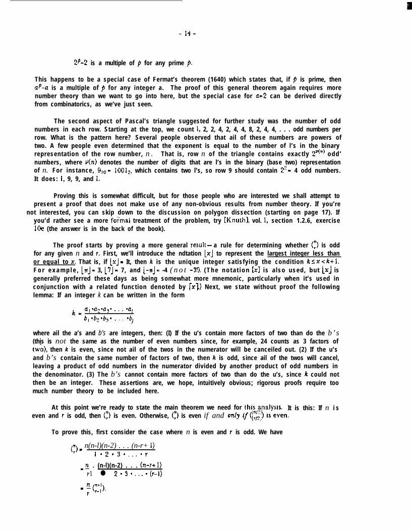
2P-2 is a multiple of p for any prime p.

This happens to be a special case of Fermat’s theorem (1640) which states that, if p is prime, thena&z is a multiple of p for any integer a. The proof of this general theorem again requires morenumber theory than we want to go into here, but the special case for a=2 can be derived directlyfrom combinatorics, as we’ve just seen.

The second aspect of Pascal’s triangle suggested for further study was the number of oddnumbers in each row. Starting at the top, we count I, 2, 2, 4, 2, 4, 4, 8, 2, 4, 4, . . . odd numbers perrow. What is the pattern here? Several people observed that ail of these numbers are powers oftwo. A few people even determined that the exponent is equal to the number of l’s in the binaryrepresentation of the row number, n . That is, row n of the triangle contains exactly 2y’n’ odd ’numbers, where v(n) denotes the number of digits that are l’s in the binary (base two) representationof n. For instance, glo = 10012, which contains two l’s, so row 9 should contain 2’ = 4 odd numbers.It does: 1, 9, 9, and I.

Proving this is somewhat difficult, but for those people who are interested we shall attempt topresent a proof that does not make use of any non-obvious results from number theory. If you’re

not interested, you can skip down to the discussion on polygon dissection (starting on page 17). Ifyou’d rather see a more fo?mai treatment of the problem, try IKnuthI, vol. 1, section 1.2.6, exercisel0e (the answer is in the back of the book).

The proof starts by proving a more general result- a rule for determining whether (:) is oddfor any given n and Y. First, we’ll introduce the ndtation lx] to represent the largest integer less thanor equal to x. That is, if [xj - It, then k is the unique integer satisfying the condition k s x < kt 1.F o r e x a m p l e , LnJ - 3, [7J - 7, and I-nJ - -4 ( n o t -3!). ( T h e n o t a t i o n [xl is a lso used, but [xJ isgenerally preferred these days as being somewhat more mnemonic, particularly when it’s used inconjunction with a related function denoted by [xl.) Next, we state without proof the followinglemma: If an integer k can be written in the form

where ail the a’s and b’s are integers, then: (I) If the u’s contain more factors of two than do the b’s(this is not the same as the number of even numbers since, for example, 24 counts as 3 factors oftwb), then k is even, since not ail of the twos in the numerator will be canceiled out. (2) If the u’sand b’s contain the same number of factors of two, then k is odd, since ail of the twos will cancel,leaving a product of odd numbers in the numerator divided by another product of odd numbers inthe denominator. (3) The b’s cannot contain more factors of two than do the u’s, since It could notthen be an integer. These assertions are, we hope, intuitively obvious; rigorous proofs require toomuch number theory to be included here.

At this point we’re ready to state the main theorem we need foreven and Y is odd, then (z) is even. Otherwise, (r) is even if and onky

It is this: If n i s

To prove this, first consider the case where n is even and Y is odd. We have

(n) E n(n-l)(n-2) . . . (n-r+ 1)r 1 *2*3*,./r

E n . (n-l)(n-2) . . . (n-r+ 1)Y 1 l 2*3*...*(r-1)

- 15-

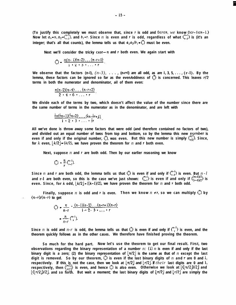
(To justify this completely we must observe that, since Y is odd and O<r<n, we know O<r-kn-I.)Now let a, =n, u2=(r$, and b,=r. Since n is even and Y is odd, regardless of what (:I:) is (it’s aninteger; that’s all that counts), the lemma tells us that ulu2/bl - (r) must be even.

Next we’ll consider the tricky case- n and Y both even. We again start with

(77) E n(n- l)(n-2) . . . (n-r+ I>’r

We observe that the factors (n-l), (n-3), . . . , (n-r+l) are all odd, as are 1, 3, 5, . . . , (r-l). By thelemma, these factors can be ignored so far as the even/oddness of (r) is concerned. This leaves r/2terms in both the numerator and denominator, ail of them even:

n(n-2)(n-4) . . . (n-r+2)2*4*6*.,/r ’

We divide each of the terms by two, which doesn’t affect the value of the number since there arethe same number of terms in the numerator as in the denominator, and are left with

h&z-l)(in-2) , . , (tn-Cy+ j)1*2*3*...+ ’

All we’ve done is throw away some factors that were odd (and therefore contained no factors of two),and divided out an equal number of twos from top and bottom, so by the lemma this new noumber iseven if and only if the original number, (f), was even. But this new number is simply ($. Since,for k even, Lk/2J - (k/2), we have proven the theorem for n and Y both even.

Next, suppose n and Y are both odd. Then by our earlier reasoning we know

Since n and Y are both odd, the lemma tells us that (r) is even if and only if (:I:) is even. But n - land r-l are both even, so this is the case we’ve just shown: (:I:) is even if and only if (‘(F$$ iseven. S ince, for k odd, lk/2J - ((k-1)/2), we have proven the theorem for n and Y both odd.

Finally, suppose n is odd and Y is even. T h e n w e k n o w n # Y, so we can multiply (:) b y- (n-r>/+) to get

(;) E n l (n-lj(n;2) ’ 3’ (n-rt,l;n-r)n - r . . * . * .

6 2.L (“;‘).n-r

Since n is odd and n-r is odd, the lemma tells us that (r) is even if and only if (“,I) is even, and thetheorem quickly follows as in the other cases. We therefore have finished proving the theorem.

So much for the hard part. Now let’s use the theorem to get our final result. First, twoobservations regarding the binary representation of a number n: (I) n is even if and only if the lastbinary digit is a zero; (2) the binary representation of [n/2J is the same as that of n except the lastdigit is removed. So by our theorem, (r) is even if the last binary digits of n a n d Y are 0 and 1,respectively. If this is not the case, then we look at ln/(rJ and [r/2J. If their last digits are 0 and 1,respectively, then (i$‘)l<Lr/2J)/2J, and so forth.

is even, and hence (r) is also even. Otherwise we look at [(Ln/2j)/2j andBut wait a moment; the last binary digits of [n/2j and Lrl2j are simply the

- 16-

next-to-last digits of n a n d Y, and the last digits of 1(172/2J)/2J and [(lr/~J)/2J are the third-to-lastdigits of n and Y, and so on. So (F) is even if, in any digit position, the binary representations of nand Y contain a 0 and 1, respectively. And what if they don’t? Then we continue discarding digitsoff the ends of the binary representations, and eventually are left with nothing but zeroes. Since(,“, - 1, which is odd, (r) must also be odd.

F o r e x a m p l e , 4510 = 101 lOi,, a n d 20io - 101002. S ince the la t ter conta ins a 1 in the fifthdigit from the right, whereas the corresponding digit in the first number is a 0, we know that (li) iseven. On the other hand, since Q. = 1 IOO,, which contains zeroes wherever 45 does, we know that(:z) is odd. (Feel free to check these results; we did!)

Okay, we’re almost done (finally!). How many numbers in row n of Pascal’s triangle are odd?This is the same as asking how many numbers Y between 0 and n (inclusive) have zeroes wherevern has zeroes in binary notation. How many such Y are there? Well, Y’S binary representation musthave zeroes wherever n’s does. Wherever n contains a 1, however, Y can contain either a I or a 0.We don’t have to worry about making Y larger than n since, even if we put l’s in uU such positions,all we get is n itself, and that’s the largest we can possibly make Y. So, letting V(n) represent thenumber of l’s in the binary representation of n, there are exactly v(n) binary digits in Y that can beeither 0 or 1, and the rest of the digits must be 0. By the product rule we have 2P(n) possible valuesfor Y, and therefore there are exactly that many odd numbers in row n of the triangle.

There’s a completely different approach to this problem. It involves looking at the pattern ofeven and odd numbers. I f we represent an odd number by a e and an even number by a blank,then the top 64 rows of the triangle look like this:

Notice that the pattern in the top 32 rows is duplicated on both sides in the next 32 rows, withnothing but even numbers in between. You might like to give some thought to how you might goabout (a) proving this replication pattern in general and (b) using it to prove that row n contains2”(“) odd numbers .

Enough already about Pascal’s triangle! Let us proceed with the course notes.

- 17-

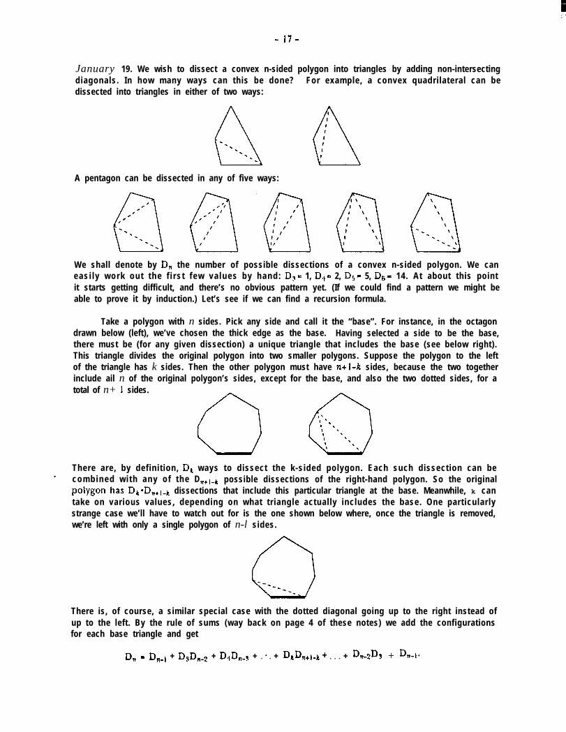
January 19. We wish to dissect a convex n-sided polygon into triangles by adding non-intersectingdiagonals. In how many ways can this be done? For example, a convex quadrilateral can bedissected into triangles in either of two ways:

A pentagon can be dissected in any of five ways:

We shall denote by D, the number of possible dissections of a convex n-sided polygon. We caneasi ly work out the f i rs t few va lues by hand: Ds = 1, D., - 2, D5 = 5, D6 = 14. At about this pointit starts getting difficult, and there’s no obvious pattern yet. (If we could find a pattern we might beable to prove it by induction.) Let’s see if we can find a recursion formula.

Take a polygon with n sides. Pick any side and call it the “base”. For instance, in the octagondrawn below (left), we’ve chosen the thick edge as the base. Having selected a side to be the base,there must be (for any given dissection) a unique triangle that includes the base (see below right).This triangle divides the original polygon into two smaller polygons. Suppose the polygon to the leftof the triangle has k sides. Then the other polygon must have n+l-k sides, because the two togetherinclude ail n of the original polygon’s sides, except for the base, and also the two dotted sides, for atotal of n+ 1 sides.

There are, by definition, Dk ways to dissect the k-sided polygon. Each such dissection can be- combined wi th any of the Dn+l-k possible dissections of the right-hand polygon. So the original

polygon has Dk*Dn+l-k dissections that include this particular triangle at the base. Meanwhile, k cantake on various values, depending on what triangle actually includes the base. One particularlystrange case we’ll have to watch out for is the one shown below where, once the triangle is removed,we’re left with only a single polygon of n-l sides.

0-- -- -- --There is, of course, a similar special case with the dotted diagonal going up to the right instead ofup to the left. By the rule of sums (way back on page 4 of these notes) we add the configurationsfor each base triangle and get

D” - D,,, + DsD,,-? + D4Dnw3 + l * l + D~Dn+l-k + l l l + Dn-zD3 + Dw

- 18-

This would be sufficient if ail we wanted to do was program a computer to evaluate D,, butfrom an aesthetic standpoint it’s not pleasing. Suppose we consider a single edge to be a polygon of2 sides-up the edge and back along the same edge-and let D2 - 1. Then our equat ion becomessomewhat more regular.

D?l = D2D,-, + DJDns2 t D4Dnw3 t l . e t DaDn+,mk t l l - t Dnm2DS t D,mlD2 (*)

Now then, this section is supposed to be about generating functions (in spite of ail that stuffabout Pascal’s triangle), so let’s make use of them. We’ll define

g(x)= D& D3x3++ Dkx’t....

(P6iya describes this as “putting ail the D’s in a ‘bag’.“) Recalling the formula for products ofgenerating functions, we take a look at the square of g.

☯g(⌧)l� = ( 2 &,⌧� ) l ( 2 IQ� >

k=? f-2

= jj2 /$ wPk+i4= D2D2x4 t(D2D3tD3D2)x5t ~~~t(D2Dm-,tD3D~-2t.~~tDm-l D2)xm+’ + l . s

But from our recursion equation (*), we know

D4 = D2D3 + D3D2..

D, = &D m-l + D3D,,,s2 t l l 9 + &l-ID2

and therefore

[g(x)]’ - D3x4 t Dqx5 t l m 6 t D,xm+’ t . a 0

- = -Dgx3 t D2x3 t D3x4 t D4x5 t l l a t D,x”‘+’ t q . 9 .

S i n c e D2 = 1, we arrive at

rg(x)lZ = -x3 t xg(x).

Now to solve this quadratic equation. (We’ll write g instead of g(x) just to make things morereadable.) P6iya’s approach was to multiply through by 4, add x2 to both sides, and move the xgterm over, with the following results.

4g2 - 4gxt x2- x2- 4x3

(Zg-x)2 - x2(1-4x)

2g - x - *x(1-4x+

g - ;r[l*(L4r)~l

- 19-

What sign do we want to choose for the *? If we choose ‘t’, then we get into trouble, because thebinomial theorem tells us that

I Wl/2 k( 1 try- 1 t c (h)Z,

L=l

so the leading term of g would be 4x( 1+ I) = x, But we know that g doesn’t have any terms ahead ofx2, so we choose ,-’ instead.

g - ix[ l-( 1-4r)bl

Now let’s take a moment to manipulate that square root some more.

( l-4$ - I t 5 ( ‘3(-4#)kk-l

= I -2x + kx2O9 #‘I(-I)(-3) . . . (1-2kt2) 4k,p(-Iys 1 *2*3*...*k

-_ w- 1 - 2xt &Ix2

2’*(- 1). 1 l 3*5* . . . l (2k-3) .pe 1 *2.3*,./k

Hence

g - tx[2x t 2 j2 [(2/2)(6/3)( lO/4) . s s ((4k-6)/k)lx’l.e

If we let kt l -n ,

g - x2 t fq [(2/2)(6/3x10/4) . . . ((4n-lO)/(n-lb”.-.

Since D, is the coefficient of x” in g, we have-

D, - (2/2)*(6/3)*( lO/4)*( l4/5)* . . . l ((4n-10)/b-18,

from which we can easily compute D, for any particular value of n. If we are computing severalconsecutive Dn, we can take advantage of the observation that

D “+, u 4n-6D ntn

and thus compute successive values in roughly constant t ime. [Note: This problem is in [MPRI,vol. 1, page 102, ex. 7, 8, and 9.1

One student included on his homework paper a continuation of the above analysis. Rewritingthe formula as

Dn a2*6*10*. . . l (4n-10)2 l 3 l 4 l . . . l (n-1) ’

E

- 20 -

he decided to look for a more compact equivalent formula. He started by extracting a factor of 2from each of the terms in the numerator, while tossing a factor of i into the denominator.

Dn a1 l 3*5* . . . l (2n-5)*2n’2

I l 2 l 3 l 4 l . . . l (n-l)

Next he multiplied the numerator by the product 2 l 4 * 6 l . . . l (2n-4), and the denominator by1 l 2 l 3 * . . . l (n-2) l 2n-2, which is, of course, the same quantity.

Dn a1*3*5, . . . *(2n-5)*2n’2 2 * 4 * 6 9,. , l (2n-4)I l 2 l 3 l 4 * . . . l (n-l) l I +3* . . . •(71-2)Q”-~

The powers of two cancel, and by rearranging the terms in the numerator we can see that

Dn =(2n-4)!

(n- l)!(n-2)!

a . (2n-3)!I2n-3 (n- l)!(n-2)!

- & l t;-fl.

Various other similar formulas are also possible, such as

This technique of multiplying by a factorial and a power of two in order to “fill in the gaps” in aproduct of odd numbers is often useful in simplifying products, and is well worth remembering.

A summary of the problem-solving rules of thumb we have encountered so far:

Cl1 Start by working out the first few “smaii” cases, and look for a pattern. If you can guess theanswer, you may be able to prove it by induction.

[21 If you can’t spot the pattern, try for a recursion formula. That is, try to come up with a way ofsolving any given instance of the problem by solving one or more smaller instances of the sameproblem.

131 If you’ve got a recursion formula but aren’t sure what to do with it, or if you’re unable to find arecursion formula at ail, try introducing a generating function whose coefficients are the valuesyou’re interested in, and see whether you can manipulate it to your advantage.

With that, we’ll move on to the next section.

People who are interested in learning more about generating functions should read IKnuthJ,vol. I, section 1.2.9. Knuth gives additional rules for manipulating generating functions, and alsodiscusses the question of convergence. For example, Itx+x2t l . q = I/( l-x) if and only if 1x1~ 1. Tworemarks f rom Knuth are par t icu lar ly worth not ing: “ . . . i t o f t e n d o e s n o t pay to worry aboutconvergence of the series when we work with generating functions, since we are only exploringpossible approaches to the solution of some problem. When we discover the solution by any means,however sloppy they might be, it may be possible to justify the solution independently” (for instanceby mathematical induction). “Furthermore it can be shown that most (if not all) of the operations wedo with generating functions can be rigorously justified without regard to the convergence of theseries.”

-21-

Principle of Inclusion and ExclusionI I

Suppose we have a set of N objects that have various properties CT, 0, “I, . . . , A. Each of the objectsmay have any or none of the properties. Let N, be the number of objects that have property c~.Some of these objects may have other properties in addition to property u; that doesn’t matter. (Infact, that’s the whole idea!) Similarly, let Ng be the number of objects that have property 0, and soon. Let N,@ be the number of objects that have both property CT and property 8, N,, the number.that have properties a and ‘Y, etc. N,b,,.h is the number of objects with atl the properties. Givenail this information, we wish to find No, the number of objects that have none of the properties.

The general formula for this is called the Principle of Inclusion and Exclusion (or sometimesPIE for short), and is the following:

No - N - No - N/j - N, - . . - - Nht N,/g t N,, t N/jr t l -. t NIh

- N,flr - Nags - a l l

.

.

.

We will eventually prove this (in two different ways, no less!), but first let’s take a look at someexamples. After all, it looks as though we need to know a heck of a lot of information in order tocompute N,,; wouldn’t it be easier to compute it directly? As we’ll see, it is sometimes much easier tocompute the various Na than it is to compute No.

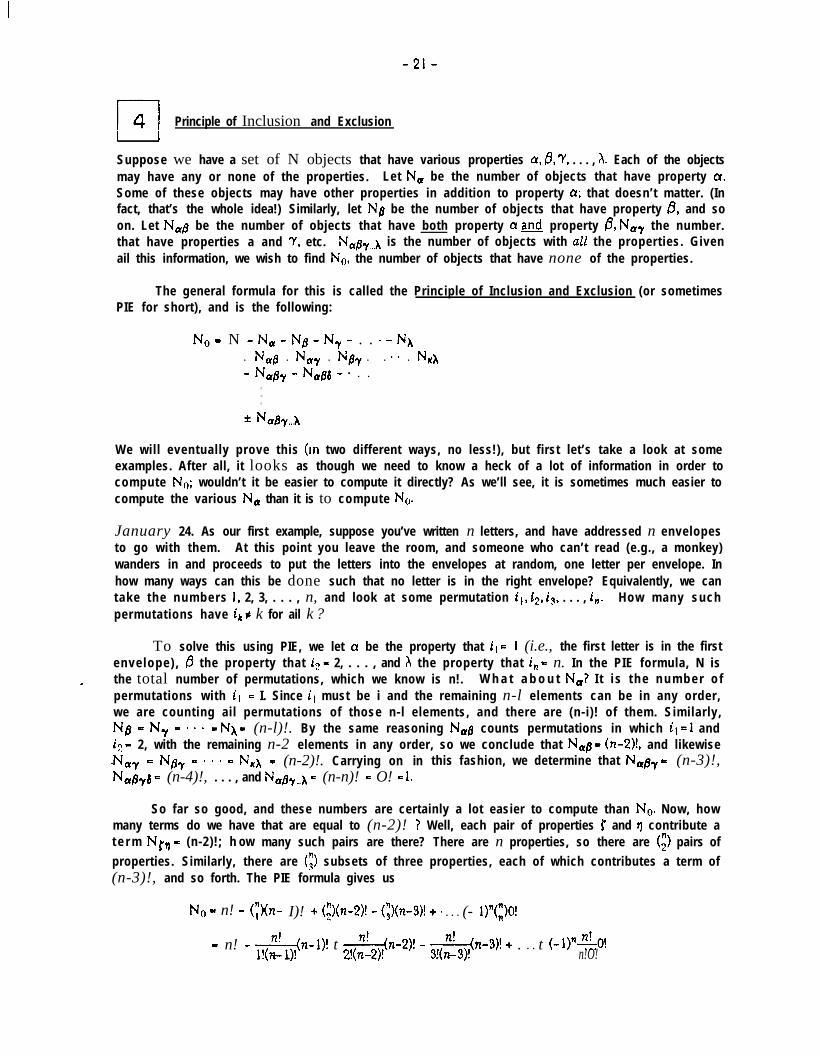
January 24. As our first example, suppose you’ve written n letters, and have addressed n envelopesto go with them. At this point you leave the room, and someone who can’t read (e.g., a monkey)wanders in and proceeds to put the letters into the envelopes at random, one letter per envelope. Inhow many ways can this be done such that no letter is in the right envelope? Equivalently, we cantake the numbers 1, 2, 3, . . . , n, and look at some permutation ill ip, i3, . . . , in. How many suchpermutations have ik # k for ail k ?

To solve this using PIE, we let a be the property that il = I (i.e., the first letter is in the firstenvelope) , 0 the property that i2 = 2, . . . , and x the property that in = n. In the PIE formula, N is

- the total number of permutations, which we know is n!. W h a t a b o u t Nd? I t i s t h e n u m b e r o fpermutations with il = I. Since i, must be i and the remaining n-l elements can be in any order,we are counting ail permutations of those n-l elements, and there are (n-i)! of them. Similarly,Ng - N, = n e - = Nh - (n-l)!. By the same reasoning Ncva counts permutations in which ii = 1 and& - 2, with the remaining n-2 elements in any order, so we conclude that Nap - (n-2)!, and likewise.N - N/jr - - a e - N,h = (n-2)!. Carrying on inNzi+ = (n-4)!, . . . , and N,or..,h = (n-n)! = O! = I.

this fashion, we determine that N,ov = (n-3)!,

So far so good, and these numbers are certainly a lot easier to compute than No. Now, howmany terms do we have that are equal to (n-2)! ? Well, each pair of properties r and t] contribute at e r m Ny, - (n-2)!; h ow many such pairs are there? There are n properties, so there are (i) pairs ofproperties. Similarly, there are (i) subsets of three properties, each of which contributes a term of(n-3)!, and so forth. The PIE formula gives us

No - n! - (YKn- I)! + @n-2)! - ($(n-3)! t 0 l l t (- l)“(:)O!

- n! - ~-j$$n-I)! t &(n-2)! - $f-$z-3)! t . l l t (- I)“-@-O!. - . . - * . - . n!O!

- 22 -

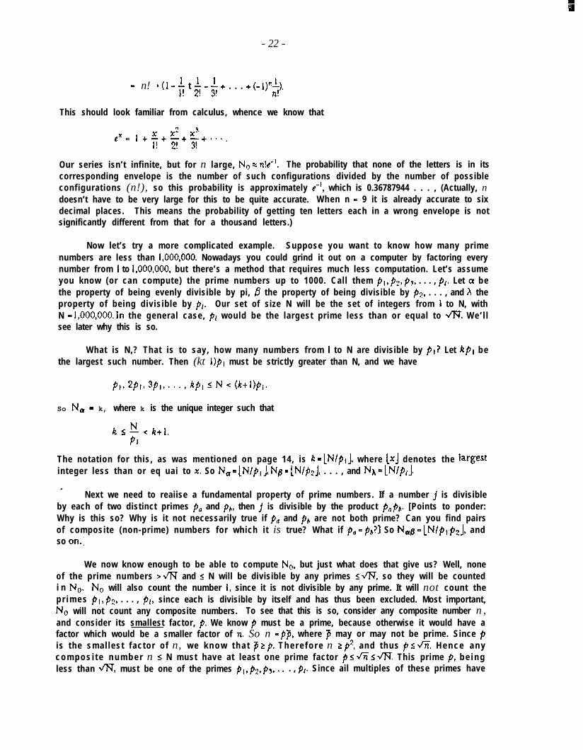
= n! + (I - h t $ - $ + . . . + (-l)+.

This should look familiar from calculus, whence we know that

e’=lt Et-t-t...*x2 x3I! 2! 3!

Our series isn’t infinite, but for n large, No z n!e”. The probability that none of the letters is in itscorresponding envelope is the number of such configurations divided by the number of possibleconfigurations (n!), so this probability is approximately e”, which is 0.36787944 . . . , (Actually, ndoesn’t have to be very large for this to be quite accurate. When n = 9 it is already accurate to sixdecimal places. This means the probability of getting ten letters each in a wrong envelope is notsignificantly different from that for a thousand letters.)

Now let’s try a more complicated example. Suppose you want to know how many primenumbers are less than l,OOO,OOO. Nowadays you could grind it out on a computer by factoring everynumber from I to 1,000,000, but there’s a method that requires much less computation. Let’s assumeyou know (or can compute) the prime numbers up to 1000. Call them pi, p2, p,, . . . , #+. Let a bethe property of being evenly divisible by pi, 0 the property of being divisible by p2, . . . , and A theproperty of being divisible by p,. Our set of size N will be the set of integers from 1 to N, withN - l,OOO,OOO. In the general case, p1 would be the largest prime less than or equal to m. We’ l lsee later why this is so.

What is N,? That is to say, how many numbers from 1 to N are divisible by pr? Let k/q bethe largest such number. Then (kt l)p, must be strictly greater than N, and we have

PI, 2p,, 3/q,. . . , kp, s N < W)p,.

So Nat - k, where k is the unique integer such that

k<%ktl.PI

The notation for this, as was mentioned on page 14, is k = LNIprJ, where [xj denotes the largestinteger less than or eq uai to x. So N, = [N/Pi j, Nc~ - [N/j+j, . . . , and Nh = [N/p/J.

Next we need to reaiise a fundamental property of prime numbers. If a number j is divisibleby each of two distinct primes PO and ph, then j is divisible by the product p,,pb. [Points to ponder:Why is this so? Why is it not necessarily true if p,, and p, are not both prime? Can you find pairsof composite (non-prime) numbers for which it is true? What if p,, = pb?] So N,p - [NIpIp2J, andso on.1

We now know enough to be able to compute No, but just what does that give us? Well, noneof the prime numbers > V% and 6 N will be divisible by any primes ,< fl, so they will be countedi n No. No will also count the number I, since it is not divisible by any prime. It will not count thep r i m e s PI, p2, . . . , pl, since each is divisible by itself and has thus been excluded. Most important,No will not count any composite numbers. To see that this is so, consider any composite number n,and consider its smallest factor, p. We know p must be a prime, because otherwise it would have afactor which would be a smaller factor of n, So n - pp, where $5 may or may not be prime. Since pis the smal lest factor of n, w e k n o w t h a t p 2 p. T h e r e f o r e n 2 p2, and thus p < 6. H e n c e a n yc o m p o s i t e n u m b e r n I N must have at least one prime factor p I fi 5 m. This prime p, b e i n gless than m, must be one of the primes p,, p2, p3,. . . , PI. Since ail multiples of these primes have

- 23 -

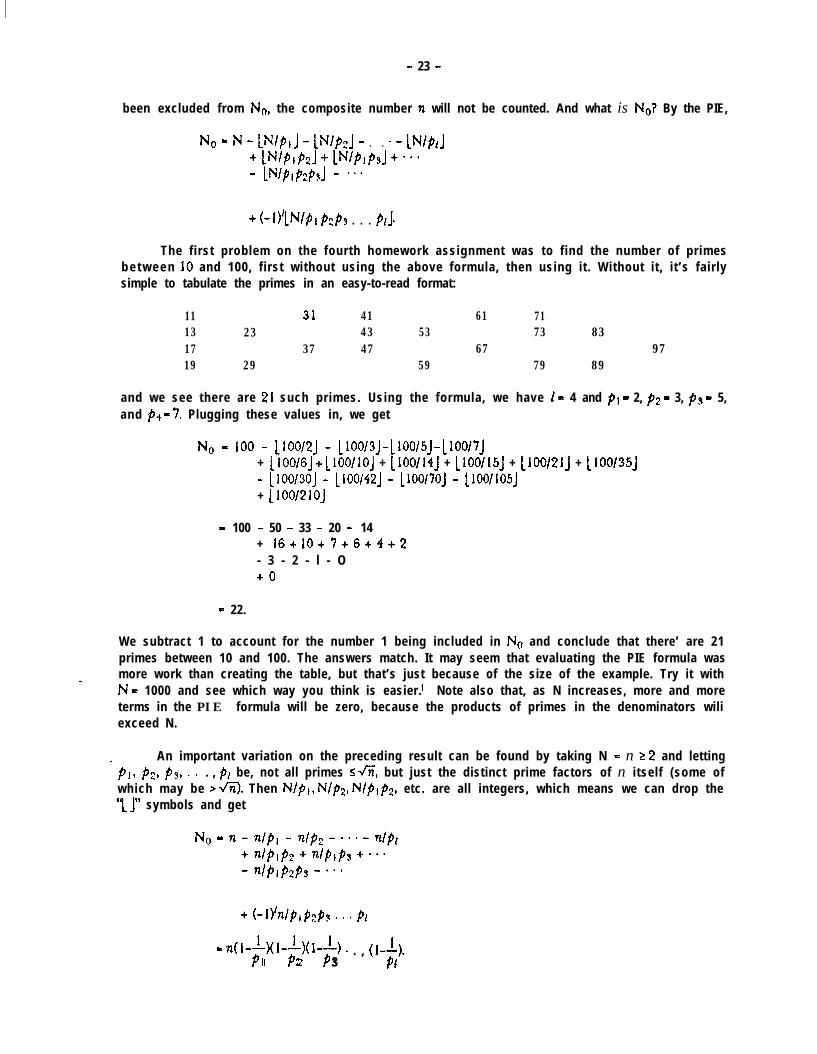
been excluded from No, the composite number n will not be counted. And what is No? By the PIE,

No = N - lN/p,☺ - ☯Nlp2] - l l 0 - lNIpl]

+lNIP,P,J+lNIP,p,J+"*- lNIPIP2Pd - ***

+ (-1)‘lNl#+ p2p, . . . p,J.

The first problem on the fourth homework assignment was to find the number of primesb e t w e e n 10 and 100, first without using the above formula, then using it. Without it, it ’s fairlysimple to tabulate the primes in an easy-to-read format:

11 31 41 61 7113 23 43 53 73 8317 37 47 67 9719 29 59 79 89

and we see there are 21 such primes. Using the formula, we have I - 4 and p, - 2, p2 - 3, ps - 5,and ps - 7. Plugging these values in, we get

No - HI0 - 1100/2J - ~100/3J - [100/5J - 1100/7J+ 1100/6J + [~oo/loJ + 1100/14J + 1100/15J + [100/21J + 1100/35J- 1100/30] - [lOO/42j - 1100/70] - 1100/105j+ ~100/21oJ

= 100 - 50 - 33 - 20 - 14+ l6+ 10+7+6+4+2- 3 - 2 - l - O+O

= 22.

We subtract 1 to account for the number 1 being included in No and conclude that there’ are 21primes between 10 and 100. The answers match. It may seem that evaluating the PIE formula was

- more work than creating the table, but that’s just because of the size of the example. Try it withN = 1000 and see which way you think is easier.1 Note also that, as N increases, more and moreterms in the PIE formula will be zero, because the products of primes in the denominators wiliexceed N.

An important variation on the preceding result can be found by taking N = n 2 2 and letting- p,, p2, ps, ’ ’ . , PI be, not all primes s fi, but just the distinct prime factors of n itself (some of

which may be > m. Then N/p,, N/p2, N/pIpZ, etc. are all integers, which means we can drop the“1 J” symbols and get

+ W’nlp&p3 . . . pi

- n(l-+I-$)(1-t). . , (l--$I 2 3 1

- 24 -

This is the number of integers from 1 to n that are relatively prime to n, i.e., have no factors incommon with n. This is sometimes called the Euler-totient function, or simply the totient; Euler’snotation for it was p(n). For example, the prime factors of 36 are 2 and 3, so

~(36) = 36(@) - I223 ’

which tells us that there are 12 numbers between 1 and 36 that are relatively prime to 36. We cancheck this: the numbers are 1, 5, 7, 11, 13, 17, 19, 23, 25, 29, 31, and 35.

Now that we’ve seen how PIE can be useful, how about a proof? We promised two proofseventually; here’s the first. Consider an object that has k of the properties. N counts it once.N,+N4+Ny+ - - l +Nh counts it exactly k times. N,b+N,,+ a . l tN,h counts it once for each way ofselecting two properties from among the k, which is just (z) times. NaaS,+Nags+ l v m counts it once

for each way of selecting three of the k properties, which ii (t) times, and so on. Altogether the PIEformula will count it 1 - k + ($ - (i) + e s .u-v,

f (i) times. But by the binomial theorem this is simplywhich is zero if k 1 I. So any object with one or more properties is counted exactly zero

times in No, which is what we want. What if k = 0, i.e., the object has none of the properties? Inthat case, N counts it once, and none of the other terms counts it at all, so No counts it exactly once.That completes our proof.

The above proof is valid, but it’s not aesthetically pleasing. The Principle of Inclusion andExclusion is an extremely important result in set theory; surely it deserves to be proved using settheory instead of combinatorics! Very well, but first we must define a bit of formal logic.

January 26. Formal logic dates back to Aristotle, and is based on syllogisms. For instance, if weaccept the premises “if A then B” and “if B then C”, where A, B, and C represent assertions, then itfollows that “if A then C”. This line of reasoning is a syllogism. We can see it pictorially. First welook at the set of objects for which A is true.

Now, “if A then B” means that anything in the set A must also be in the set B, as shown below.

Similarly, anything in the set B must also be in the set C:

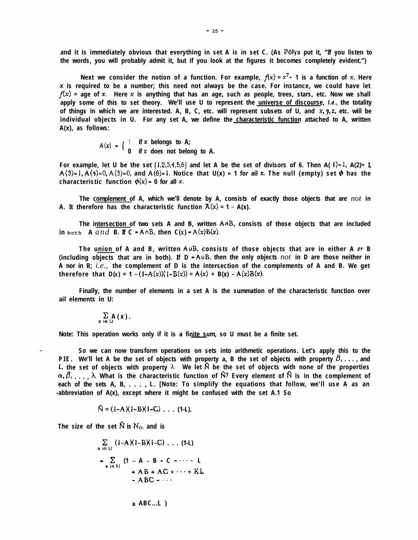
- 25 -

and it is immediately obvious that everything in set A is in set C. (As Polya put it, “If you listen tothe words, you will probably admit it, but if you look at the figures it becomes completely evident.“)

Next we consider the notion of a function. For example, f(x) = x2- 1 is a function of x. Herex is required to be a number; this need not always be the case. For instance, we could have letf(x) = age of x, Here x is anything that has an age, such as people, trees, stars, etc. Now we shallapply some of this to set theory. We’ll use U to represent the universe of discourse, i.e., the totalityof things in which we are interested. A, B, C, etc. will represent subsets of U, and X, y, Z, etc. will beindividual objects in U. For any set A, we define the characteristic function attached to A, writtenA(x), as follows:

A(x) = { 1 if x belongs to A;0 if x does not belong to A.

For example, let U be the set (1,2,3,4,5,6j and let A be the set of divisors of 6. Then A( l)=l, A(2)= I,A(3)=1, A(4)=0, A(5)=0, and A(6)=1. Notice that U(x) = 1 for ail x. The nul l (empty) set $ has thecharacteristic function 6(x) = 0 for all X.

The complement of A, which we’ll denote by A, consists of exactly those objects that are not inA. It therefore has the characteristic function A(x) = 1 - A(x).

The intersection of two sets A and B, written AnB, consists of those objects that are includedin both A and B. If C = AnB, then C(X ) = A(x)B(x).

The union of A and B, wr i t ten AuB, consists of those objects that are in either A OY B(including objects that are in both). If D = AuB, then the only objects not in D are those neither inA nor in B; i.e., the complement of D is the intersection of the complements of A and B. We gettherefore that D(X ) = 1 - (I-A(%))( I-B(x)) = A(x) + B(x) - A(x)B(x).

Finally, the number of elements in a set A is the summation of the characteristic function overail elements in U:

c A ( x ) .x rn U

Note: This operation works only if it is a finite sum, so U must be a finite set.

- So we can now transform operations on sets into arithmetic operations. Let’s apply this to theP I E . We’ll let A be the set of objects with property a, B the set of objects with property 0, . . . , andL the set of objects with property A. We let fi be the set of objects with none of the propertiesa, 6, . . . , A. What is the characteristic function of 147 Every element of fi is in the complement ofeach of the sets A, B, . . . , L. [Note: To simplify the equations that follow, we’ll use A as an

-abbreviation of A(x), except where it might be confused with the set A.1 So

fl = (I-A)(l-B)(l-C) . . . (1-L).

The size of the set fi is NO, and is

c (I-A)(l-B)(i-C) . . . (1-L)x In U

= .zu (1 - A - B - C - se*- L

+AB+ACt~~~tKL-ABC-...

* ABC...L )

- 26 -

= c 1 - c A - c B -..ax in U x In U x in U

txzUAB +..e..

i r iFu ABC.. .L .

Since r ,zu AB, for example, is the size of the set AnB, which in turn is the set of objects with both

properties a and 0, this is the same as N,B in our earlier notation. So we find that

Cx in U

n(x) = No = N - N, - Ng - N, - 0.. - NX

t N,4 t N,, + N/jr + - l l + N,⌧

- N,flr - Nap - . . *

.

.

.

That’s it for PIE. We’ll be seeing more of it later on.

q -_5 Stirling Numbers

We now come to a somewhat esoteric set of numbers called Stirling numbers (after mathematician,James Stirling). There are two kinds of Stirling numbers; they are called, appropriately enough,Stirl ing numbers of the first kind and Stirlinp numbers of the second kind. We’ll start with thesecond kind.

We def ine SL to be the number of ways to divide a set of size n into k n o n - o v e r l a p p i n g ,non-empty subsets whose union is the whole set. Such a division is called a partition into k subsets.

Incidentally, you should be warned that there is no “standard” notation for Stirling numbers.The notation we’ll be using is one of the more common ones, but if you read any texts on thissubject you should be prepared to see various other notations.are $ (confusing!) and {l].

Among the more common notations

Let’s look at a few sample values to get a feel for these numbers. First we observe that Si = 0unless 1 s k I n. (Obviously, we cannot partition n objects into fewer than 1 set, nor can we formmore than n subsets and still have all the sets non-empty.) We also observe that, if k = 1, there’sonly one way to “divide” the set. The same is true if k = n; each object must belong to a differen?tsubset, and the order of the subsets is not being considered. So the first complicated value is S,.T h e s e t {a,b,c) can be d iv ided in to {a,b) and {c), or (a,c) and (b), or (b,c} and (a) . S o S: = 3 . W h a tabout Sl? If we are going to partition a set of 4 objects into 2 subsets, the subsets must be either ofsizes 3 and 1 or of sizes 2 and 2. In the first case, there are 4 choices for the element in the set ofsize 1. The second case is a bit tricky-we’re tempted to say that there are (i) = 6 choices for thepair of objects to be placed in the first subset, but this would be incorrect. Choosing (a,b) for thefirst subset is equivalent to choosing (c,n}, since the order of the two subsets is irrelevant. Thecorrect way to count these partitions is to look at some element, say a. It must be in one or the othersubset, and it doesn’t matter which since the two are symmetrically equivalent. Whichever it’s in,there are 3 choices for the other element of that subset. Having made that choice, we’ve completelydetermined the partition, since the other two elements must go in the yther subset. So there arethree partitions of 4 objects into two subsets of size 2. Altogether then, S, = 7.

- 27 -

For Sl, the subsets must be of sizes 2, 1, and 1. There are (i) = 6 ways to choose the subset ofsize 2, and each such choice completely determines the partition. (Note that, unlike the situationencountered in the previous paragraph, all 6 cases are now different.) So S: = 6.b

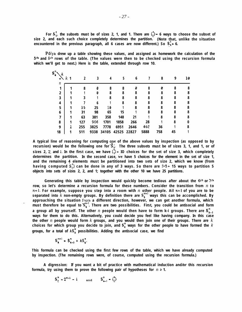
P6lya drew up a table showing these values, and assigned as homework the calculation of the5th and 6th rows of the table. (The values were then to be checked using the recursion formulawhich we’ll get to next.) Here is the table, extended through row 10.

Sii\ k 1 2 3 4 5 6 7 8 9 18n1 1 8 0 8 8 0 8 0 8 82 1 1 8 8 8 8 8 8 8 83 1 3 1 8 8 8 8 8 8 84 1 7 6 1 8 8 8 8 8 85 1 15 25 10 1 8 8 8 8 86 1 31 98 65 15 1 8 8 8 87 1 63 381 358 148 21 1 8 8 88 1 127 9G6 1701 1858 266 28 1 8 09 -1 255 3825 7778 6951 2646 4G2 36 1 8

18 1 511 9338 34105 42525 22827 5888 758 45 1

A typical line of reasoning for computing o;e of the above values by inspection (as opposed to byrecursion) would be the following one for S,. The three subsets must be of sizes 3, 1, and 1, or ofsizes 2, 2, and 1. In the first case, we have (:) = IO choices for the set of size 3, which completelydetermines the partition. In the second case, we have 5 choices for the element in the set of size 1,and the remaining 4 elements must be partitioned into two sets of size 2, which we know (fromh a v i n g c o m p u t e d Sl) can be done in any of 3 ways. So there are 3*5 = 15 ways to partition 5objects into sets of sizes 2, 2, and 1; together with the other 10 we have 25 partitions.

Generating this table by inspection would quickly become tedious after about the 6th or ‘7throw, so let’s determine a recursion formula for these numbers. Consider the transition from n t ont I. For example, suppose you step into a room with n other people. Ail nt I of you are to beseparated into k non-empty groups. By definition there are Sit’ ways this can be accomplished. By

- approaching the situation fr;+y a different direction, however, we can get another formula, whichmust therefore be equal to S, . There are two possibilities. First, you could be antisocial and forma group all by yourself. The other n people would then have to form k-i groups. There are S%,ways for them to do this. Alternatively, you could decide you feel like having company. In this casethe other n people would form k groups, and you would then join one of their groups. There are kchoices for which group you decide to join, and S: ways for the other people to have formed the kgroups, for a total of kSi possibilities. Adding the antisocial case, we find

S;+’ = S;-, t kS,“.

This formula can be checked using the first few rows of the table, which we have already computedby inspection. (The remaining rows were, of course, computed using the recursion formula.)

A digression: If you want a bit of practice with mathematical induction and/or this recursionformula, try using them to prove the following pair of hypotheses for n L 1.

s,: E y-1 - 1 and SE-, = (i)

- 28 -

January 31. As an example, suppose we have k different colors of paint, and we wish to paint nhouses. (Each house is to be painted a single color.) In how many ways can we do this?

The first house can be painted in any of k di f ferent ways. Independent of the color wechoose for the first house, the second house can also be painted in any of k different ways, and soon for each house. So there are k*k*k* . . . l k = k” ways. But this includes cases where not ail of thek colors are used; e.g., all the houses might be painted blue. How many ways actually use all kcolors?

This looks like a job for PIE. Let CT be the property that no house is painted with the 1stcolor, fi the property that no house is painted with the 2nd color, . . . , and x the property that nohouse is painted with the kth color. We want the number of ways to paint the houses such that allthe colors are used, i.e., color assignments with none of the properties a, 0, . . . , A. We recall fromthe previous section that

N we know is k”. Nar is the number of ways to paint the houses without using color *l. Since eachhouse can be any of (k-l) colors, No = (k-l)“. The same goes for No, N,, etc., for a total of k s u c hterms. Similarly, N,4 = (k-2)“, since each house can be any of (k-2) colors. There are (i) suchterms. Carrying on in this fashion, we find

No = k” - (;)*(k-1)” t @(k-2)” - @(k-3)” t a 9 l t (- l)‘(:)*O”.

As usual, we’ll check this formula on a few special cases, just to see whether we’ve made anyobvious mistakes. For instance, if k = 1 and n 2 1, there should be only one way to paint the housesusing the s ingle ava i lab le co lor . The formula y ie lds No = 1’ - (#On = 1 . I t checks. How aboutn = 1 and k L 2? There’s no way to paint one house so as to use two or more colors (since we’rerestricting ourselves to a single color per house), so the formula should yield zero.

N,, - k - (+(k- 1) t (@k-2) - @(k-3) + 9 l 9 t (-l)‘(;)*O.

= ;(; (- 1 )Yf)e(k-S)

* 5’ k!(lt-J) (-1)’370 s! (k-J)!

[the last term In the previous line = 0 and is omitted from the summattonl

u y ke(k;‘)+l)ss=o

= k ;; (‘;‘)*(-1)’I

= k 9 ( 1 - l ) “ ’

- 29 -

So if k 2 2, this indeed comes out zero. Note that, if k = I, we once again find ourselves relying onO0 being equal to 1. As a final special case, consider tl = 0. Since 0’ = 1, the formula turns into

No - 1 - (;, + (;, - (“,, + a - a + (-I)~(:).

= ( l - l ) ‘ ,

which equals zero i f It 2 I. Since there is no way to paint zero houses so as to use one or morecolors, this checks. If k - 0, we find there is exactly one way to paint zero houses using zero colors,which sounds reasonable, too.

Okay, so the formula looks good. Let’s approach the problem in a different way and see if wecan learn anything. When we paint the n houses, we could do it by first partitioning the housesinto It sets-the set of houses painted the 1st color, the set painted the 2nd color, etc. We require thateach of these sets be non-empty, since each color is to be used on at least one house. Thereforethere are Si ways to partition the houses. Having done so, we then have K! ways to assign the k

colors to the k sets, so there are Sz*k! ways to paint the houses using ail k colors. But this meansthat

S;*k! = k” - (+(k- 1)” + (942-2)” - (;)+z-3)” + . . . + (-#(:).o”. (*O

(Checking this formula for n = 5 and 6 was assigned as homework. It is a fairly straightforwardprocedure given the table for SI which we produced earlier, so we won’t go into it here.)

For our next bit of fun, let’s try to turn this into a generating function. It turns out that agenerating function in which SI is the coefficient of 2” is awkward. This often happens when thecoefficients increase particularly rapidly; though we don’t normally need to worry about whether agenerating function converges, it helps if it converges for at least settle non-zero values of x. If thecoefficients of the generating function are growing faster than the powers of z can shrink (for r<l>,then it will not converge (i.e., the sum will be infinite). When this sort of problem arises, it oftenpays to divide the coefficients by something that itself grows very quickly, namely n!. So, given aparticular value of k, we let n vary and take the summation

-S i n c e SL I: 0 for 0 I n < It and since the formula (*) holds there also, we can extend the summationto start at zero instead of k.

Remembering that

we get

O” XRc - - i+X+-+2+...-ex,x2

n=O n! l! 2! 3!

. . . t (- 1 )k(:)eol

- 30-

That’s enough for now with regard to Stirling numbers of the second kind. Let’s take a lookat the first kind. Those of the second kind were defined using partitions of a set; those of the firstkind are defined using cycles of a permutation. So it’s time to define a few more terms.

Consider any permutation of n objects. We’ve been thinking of it as an ordering of theobjects, one of n! possible orderings. We can instead represent it by writing the numbers 1 throughn to denote the n objects, and writing below k the number of the lath element of the ordering. Forinstance, if the first element of the set is placed fifth in the particular permutation, then we write 1below 5. The general notation for this will be

(1 2 3 4 . . . ryeii i2 is i4 . . . in

For example, for n - 6, one possible permutation is

Here’s the important concept: We can think of this as a function mapping the set (1,2,3,4,5,6)onto itself. For this particular permutation, fcl) = 3, f(2) = 5, . . . , and f(6) = 1. Th is funct iona linterpretation of permutations will become more significant in the next section. For now, we’re onlyinterested in the cycles of the function. These are easier to understand if we look at the functiongraphically. Extending our earlier example, we can represent the function f by using arrows toindicate the operation; e.g., 1 --t 3 indicatesfil) - 3.

2

The graph becomes easier to read if we separate it into its independent parts.

6

Each of these parts is called a cvcie. A cycle of k elements (also called a “cycle of order &“) representsa portion of th e permutation that, if applied k times, restores the original ordering to those elements.In our example, there is a cycle of order 3 containing the elements 1, 3, and 6. This tells us thatml>)) - 1, fvv(3))) - 3, and m6))) - 6. Similarly, fv(2)) - 2, f(f(5)) = 5, and f(4) - 4. Note theadvantage of thinking of the permutation as a function, which permits us to perform it multipletimes, an operation that might be hard to visuaiise in terms of reordering elements of a set. (As wementioned before, we’ll see more of this in the next section.)

A permutation can be completely specified by showing the cycles. The usual notation for this

- 31 -

involves putting each cycle’s elements inside a set of parentheses; our example would be written as

(1 3 6)(2 5)(4).

This represents the mapping

(I --t 3, 3 +- 6, 6 -+- I) (2 -t 5, 5 --t 2) (4 -t 4)

Note that the cycle notation is not unique. The above permutation could also be written as, forinstance, (2 5)(4)(3 6 1). But (2 5)(4)(3 1 6) is a different permutation, since it implies 3 -+- 1instead of 1 +- 3.

The number of permutations of n elements that consist of precisely k cycles is the Stirlingnumber of the first kind, which we’ll write as & (Another common notation is [il. Also, somereferences use S for Stirling numbers of the first kind and J for those of the second kind, and otherreferences use u or other esoteric characters. As Knuth puts it, “There is absolutely no agreementtoday on notation for Stirling’s numbers.” Any good reference will therefore go to great pains todescribe the notation being used; look for this description any time you’re reading up on Stirlingnumbers.)

To repeat then, we’ll be using A,” for Stirling numbers of the first kind. Let’s look at a fewexamples. For instance, when n = 1, the:e is only one permutation, namely 1 +- 1, and it has asingle cycle (of order one). Therefore 8, = 1 . When n = 2 , there are two permutat ions. One ofthem has 1 --t I and 2 --t 2; in cycle notation this is (l)(2). The other has 1 +- 2 and 2 +- 1,which in cxcie nptation is (1 2). So there is one permutation with one cycle and one with two cycles,a n d t h u s 8; = ,& - 1 .L.

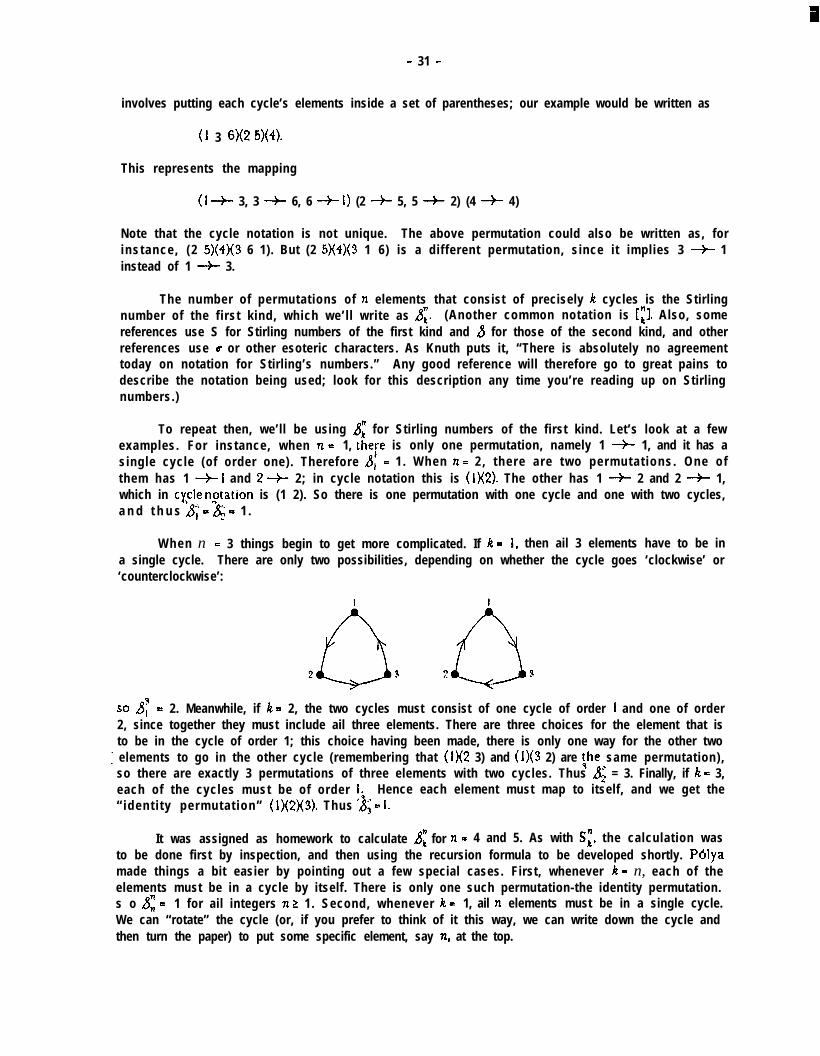
When n = 3 things begin to get more complicated. If 12 - 1, then ail 3 elements have to be ina single cycle. There are only two possibilities, depending on whether the cycle goes ‘clockwise’ or‘counterclockwise’:

so s; = 2. Meanwhile, if ft = 2, the two cycles must consist of one cycle of order 1 and one of order2, since together they must include ail three elements. There are three choices for the element that isto be in the cycle of order 1; this choice having been made, there is only one way for the other two

; elements to go in the other cycle (remembering that (1)(2 3) and (1)(3 2) are the same permutation),so there are exactly 3 permutations of three elements with two cycles. Thus ,& = 3. Finally, if k = 3,each of the cycles must be of order l6 Hence each element must map to itself, and we get the“ ident i ty permutat ion” (l)(2)(3). Thus A; = 1.

It was assigned as homework to calculate fi: for n = 4 and 5. As with SL, the calculation wasto be done first by inspection, and then using the recursion formula to be developed shortly. Pdiyamade things a bit easier by pointing out a few special cases. First, whenever k = n, each of theelements must be in a cycle by itself. There is only one such permutation-the identity permutation.s o 8; = 1 for ail integers n 1 1. Second, whenever & = 1, ail n elements must be in a single cycle.We can “rotate” the cycle (or, if you prefer to think of it this way, we can write down the cycle andthen turn the paper) to put some specific element, say n, at the top.

- 32 -

Having established this fixed point of view, we can then place the remaining n-i elements in anyorder. Each such cycle will be different from the others, so we find that 8; = (n-l)! for ail n 2 1.

The third and last ‘hint’ supplied to aid in doing the homework was that, if we count ail thepermutations with one cycle, and also those with two cycles, and those with three, four, etc., we endup counting all permutations. But we know how many permutations there are altogether. Hence

for ail positive integers n.

As before, we won’t go into ail the details here regarding the computation by inspection of 8:for n = 4 and 5. One typical value is 4, which we can compute as follows. The two cycles musteither be one of order 3 and one of order 2, or else one of order 4 and one of order 1. In the lattercase, there are 5 choices for the element in the order-l cycle, and for each choice there are (by ourearlier reasoning regarding &) (4-l)! = 6 ways to arrange the order-4 cycle. In the other case, wehave (l) = 10 choices for the order-2 cycle, and for each choice there are 2 ways to arrange the otherelements in the order-3 cycle. So 4 = 5’6 t lOa2 = 50. The following table shows fi: for n 5 8.

4 it\n1234a5678

1 2 3 4 5 6 7 8

1 0 8 8 8 8 0 81 1 8 8 6 8 8 82 3 1 8 0 8 0 86 11 6 1 8 8 8 8

24 58 35 18 1 8 8 8128 274 225 85 15 1 8 87 2 8 1 7 6 4 1 6 2 4 735 175 21 1 8

5 8 4 8 1 3 8 6 8 1 3 1 3 2 6 7 6 9 1 9 6 8 322 28 1

Now let’s try to find a recursion formula for these numbers. Suppose you enter a room andfind n people already arranged in cycles. If you want to be alone, you can form a cycle by yourself.If there are to be k cycles altogether, then the other n people must be in k-1 cycles, and there are

X-l ways this can be done. But if you want to be sociable, you can join an existing cycle. In thiscase there must be k cycles already formed, and there are 8; ways this can be done. For each sucharrangement, how many ways are there for you to join one of the cycles? Well, for any particularcycle, you could step between any adjacent pair of people, so there are as many ways for you to joinas there are people already in the cycle. So ail told there are n ways for you to join the other npeople . (Basica l ly , you can step in f ront o f any of the n people.) Adding the two cases, we get therecursion formula

- 33 -

Compare this to the recursion formula for S:

Note the different coefficients on the second terms. You might also want to test out the formula for18 by using it to prove the special cases JF = (n-l)! and &-, - (:).

February 2. We’ve looked at a generating function for Stirling numbers of the second kind. Whatabout those of the first kind? For any particular value of n, we’ll define

(Note that we’re taking n as fixed this time instead of k. We could also let k be fixed and sum overail values of n, getting a very different generating function, but we won’t go into that in these notes.)We’ll start by looking at the first few such functions and trying to spot a pattern.

g,(x) = xg&c) = x t x2g&x) i.2 2 X t 3x2 t 2

Hmm, not much of a pattern there, or is there? Let’s try factoring them.

grw = x =Xg&c) = x t x2 = x(1+x)g&d = 2% + 3x2 t xJ = x(1+x)(2+x)

Ah, that’s much better! It looks as though

g,(x) = x(x+ l)(xt2)(x+3) . . . (xtn-I).

Let’s see if we can prove this conjecture. Some parts of it we can check at once. The coefficient ofx” will always be 1, which is indeed 4,“. The coefficient of 3c will be I l 2,3* . . . *(n-l) = (n-l)!, whichi s $y. So it looks good; how do we prove it in general? Well, it’s correct for n = I, 2, and 3, so let’s

- try mathematical induction. W e ’ l l a s s u m e t h a t g,(X) - x(x+ 1)(x+2) . . . (x+n-I) for some value of fitand try to prove that g,+,(x) = x(x+ 1)(x+2) . . . (xtn).

⌧ ( ⌧ + 1)(⌧+2) l l l (xtn) = [g,(x)J*(z+n)

S i n c e n& = n*(n-l)! = n! = &*‘, and JI = 1 = &$ and (most important ly ) ,&+n& = &*I by t h erecursion formula, we find

X(x+ 1)(x+2) . . . (xtn) = S:*‘X + g+‘x2 + &+I$ + . . . + &+txn + J’~~Xn+t

- 34 -

This generating function is most often shown in a slightly different form, which we can deriveby substituting (-X) for x and multiplying both sides by (-1)“:

(-l)“~;<-X> t (-l)“&X)? t * * ’6. t (-l)‘$$(-x)” = ( -x ) ( -x+ 1)(-x+2) . . . (-xtn- 1)*(-l)”

I ~3)” - .8~-,x”-’ t &2xn-2 - * l . t (- 1)“~‘@ = x(x-1)(x-2) . . . (x-n+ 1) I

Note that the right-hand side can be rewritten as (z)n!.

Let’s go back for another look at SL. Suppose we’re painting n houses and have x colorsavailable. In how many ways can we do this, not neceJsarily using ail x colors? One way to look atit is to say that there are x choices for the color of the first house, and independent of that there arex choices for the color of the second, and so on for a total of xn possibilities. Another way to took atit is to start by asking how many ways there are to paint the houses using exactly one color fromamong the x colors available. Obviously there are x ways. How many ways use exactly two colors?We first partition the houses into two subsets. We then choose any color (x possibilities) and paintail the houses in the first subset using that color. We then pick any other color (x-l possibilities)and use it to paint the remaining houses. So there are S$&c-1) ways to paint the houses usingexactly two of the x colors. Similarly, we can deduce that there are Syx(x-1)(x-2) ways to paint themusing exactly three colors, and so forth. We conclude that:

I xn = SIX t S$t(x- I) t Szx(x-1)(x-2) t e e . t SIx(x-1Xx-2) . . . (x-n+ 1) I

Compare this formula with the previous one; the two are in some vague sense symmetric. Thefirst one represents numbers of the form (i)k! in terms of powers of x, whereas the second representspowers of x in terms of numbers of the form (i)k!. It was in this form that Stirling originallydeveloped these numbers. The expressions (i)k! play a significant role in interpolation methods,which is one reason why Stirling numbers are considered worth investigating.

That’s it for Stirling numbers, and section 5 of these notes. For more information on Stirlingnumbers, you may refer to [P-St] vol. 1, pp. 42-45 and pp. 224-229. (The former pages containvarious exercises, while the latter discuss the solutions.)

r-l6 P6lya’s Theory of Counting

February 2. P6iya’s tit le for this section was actually “Counting Configurations Non-Equivalentwith Respect to a Given Permutation Group”. Just about everybody else calls it “P6iya’s Theory ofCounting”. This latter title is somewhat easier to remember, though not as indicative of the content.We’ll stick to the simpler title; for the content, read on!

Since we’re going to be dealing in this section with permutation groups, we’ll start by coveringa b i t o f Group Theory . You’ll recall from the previous section that we have ceased thinking of apermutation as merely an ordering of n objet!. It can be more generally thought of as a function, atransformation of n elements. For instance, (!, G f) is a function, call it f(x), such that f( 1) = 2,f(2) = 3,and f (3 ) = 1. A second permutation, say (, J 2 ,’ “j represents another function, g(x), such that g(l) - 1,g(2) = 3, and g(3) = 2. We shall use the notation

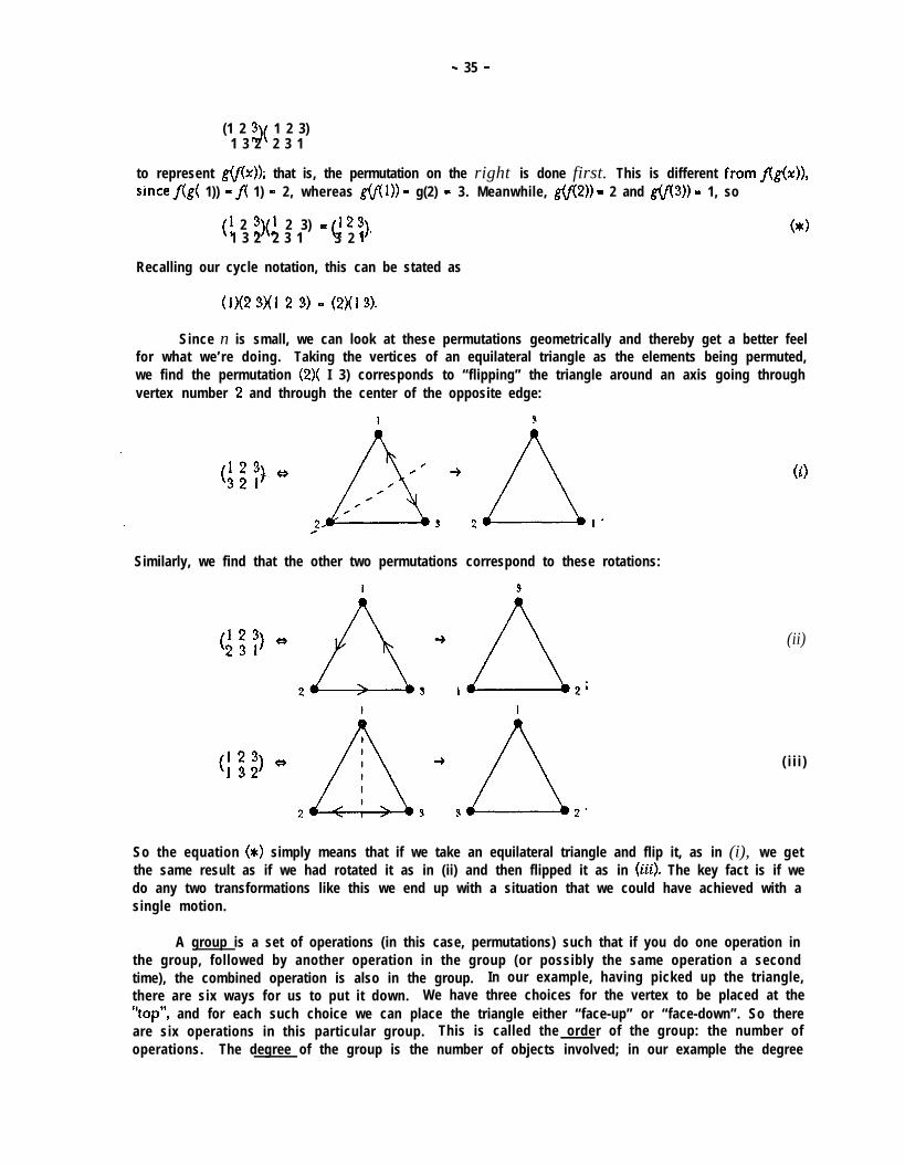
- 35 -

(1 2 3)( 1 2 3)1 3 2 2 3 1

to represent g(f(x)); that is, the permutation on the right is done first. This is different from&(x)),sinceflg( 1)) = f( 1) = 2, whereas Ml)) = g(2) = 3. Meanwhile, gv(2)) = 2 and m3)) - 1, so

(1 2 3x1 2 3) e (1 2 3).1 3 2 2 3 1 3 2 1

(*c)

Recalling our cycle notation, this can be stated as

(1)(2 3)(1 2 3) = (2X1 3).

Since n is small, we can look at these permutations geometrically and thereby get a better feelfor what we’re doing. Taking the vertices of an equilateral triangle as the elements being permuted,we find the permutation (2)( I 3) corresponds to “flipping” the triangle around an axis going throughvertex number 2 and through the center of the opposite edge:

Similarly, we find that the other two permutations correspond to these rotations:

(0

(ii)

( i i i )

So the equation (*) simply means that if we take an equilateral triangle and flip it, as in (i), we getthe same result as if we had rotated it as in (ii) and then flipped it as in (iii). The key fact is if wedo any two transformations like this we end up with a situation that we could have achieved with asingle motion.

A group is a set of operations (in this case, permutations) such that if you do one operation inthe group, followed by another operation in the group (or possibly the same operation a secondtime), the combined operation is also in the group. In our example, having picked up the triangle,there are six ways for us to put it down. We have three choices for the vertex to be placed at the“top”’ and for each such choice we can place the triangle either “face-up” or “face-down”. So thereare six operations in this particular group. This is called the order of the group: the number ofoperations. The degree of the group is the number of objects involved; in our example the degree

- 36 -

is three.

Of the six operations in this particular group, one involves “standing still”:

(’ 23)123 e 2A3+2Ay.Three operations involve holding a vertex fixed and interchanging the other two (as in (i) and (iii)on the preceding page), and the remaining two operations involve rotation 120” in one direction orthe other about the center (as in (ii)). So we have one case of the form (a)(b)(c) in cycle notation,three cases of the form (a)(b c), and two of the form (a b c). We shall represent a cycle of order k b ythe variable jh. (Some texts use other notations.) A combination of cycles will be represented by aproduct; hence (1)(2 3) is denoted by flf2 and (l)(2)(3) by fl ‘. Finally, we add together the productscorresponding to the various permutations, and divide by the total number of permutations in thegroup. Since there is one permutation of the form fl ‘, three of the form flf2, and two of the formfs, we come up with

This is called the cycle index of the permutation group. We’ll be defining this more precisely lateron. It is perhaps the most important single concept in this course.

February 7. As a somewhat more interesting example, consider the rotations of a regular hexagon.A hexagon can be rotated in various ways such that it “coincides with itself”. By “coincides” wemean that, if the hexagon is not iabeiied in some way, there is no way to distinguish the originalposition from the rotated position. Thus, for example, we do not include the rotation

On the other hand, we can rotate the hexagon as indicated by the arrows (below left), or we can liftit out of the plane and rotate it 180’ about either of the axes shown in dotted lines (below centerand right).

- 0 1 . .We wish to find the cycle index for this group. Well, to begin with, how many operations are

in the group ? That is, in how many different ways can we rotate a regular hexagon such that itcoincides with itself? We pick some vertex and rotate the hexagon to place that vertex in theposition of our choice; there are six possible positions. Having chosen where to place that vertex,we still have a decision left to make-we can place the hexagon “face up” or “face down”. That is,we could flip the hexagon over or we could choose not to. Hence the totat number of positions for

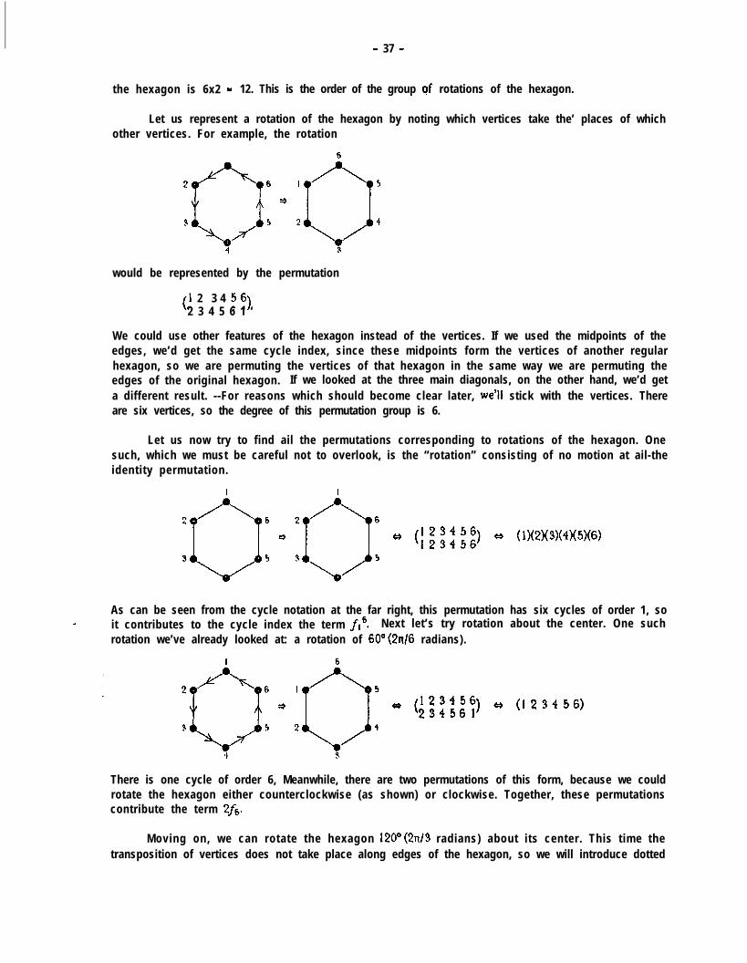
- 37 -

the hexagon is 6x2 = 12. This is the order of the group crf rotations of the hexagon.

Let us represent a rotation of the hexagon by noting which vertices take the’ places of whichother vertices. For example, the rotation

2

s

:I’z4

6 I

5 2

6

0

5

4

3

would be represented by the permutation

(1 2 3 4 56)2 3 4 5 6 1 ’

We could use other features of the hexagon instead of the vertices. If we used the midpoints of theedges, we’d get the same cycle index, since these midpoints form the vertices of another regularhexagon, so we are permuting the vertices of that hexagon in the same way we are permuting theedges of the original hexagon. If we looked at the three main diagonals, on the other hand, we’d geta different result. --For reasons which should become clear later, we% stick with the vertices. Thereare six vertices, so the degree of this permutation group is 6.

Let us now try to find ail the permutations corresponding to rotations of the hexagon. Onesuch, which we must be careful not to overlook, is the “rotation” consisting of no motion at ail-theidentity permutation.

As can be seen from the cycle notation at the far right, this permutation has six cycles of order 1, so- it contributes to the cycle index the term fl’. Next let’s try rotation about the center. One such

rotation we’ve already looked at: a rotation of 60” (2n/6 radians).

There is one cycle of order 6, Meanwhile, there are two permutations of this form, because we couldrotate the hexagon either counterclockwise (as shown) or clockwise. Together, these permutationscontribute the term 2fs.

Moving on, we can rotate the hexagon 120” (2n/3 radians) about its center. This time thetransposition of vertices does not take place along edges of the hexagon, so we will introduce dotted

- 38 -

lines to indicate where the vertices end up.

6 6

(1 3 5)(246)

As before, we could perform this rotation either clockwise or counterclockwise, so we get the term2f 32.

Finally, we could rotate the hexagon 18OO. In this case, there is no choice of clockwise versuscounterclockwise, since rotation in either of the two directions yields the same permutation.

Here we end up with three pairs of vertices being interchanged. Each such interchange is a cycle oforder 2, so we get the termf2?

So much for rotations about the center, We could also rotate the hexagon about an axisdrawn through two opposing vertices. In this case the rotation must be through 180’; otherwise thehexagon will not end up in the same plane surface in which it started. (We could, of course, rotateit O”, but this is the same as a 0’ rotation about any other axis, so we’ve already counted that case.)

d

4 4

Here the axis was taken to be through the vertices iabeiied I and 4. We couldchosen it to be through any other pair of opposing vertices. Since there are sixthere are three distinct pairs of opposing vertices. Each yields a permutat ion.

just as easily havevertices altogether,that , l ike the one

shown above, contains two cycles of order 1 and two of order 2. Hence we get the term 3fr2fz2.

There’s one other type of axis to consider, one drawn through the midpoints of two opposingedges. Again we must rotate the hexagon through 180’.

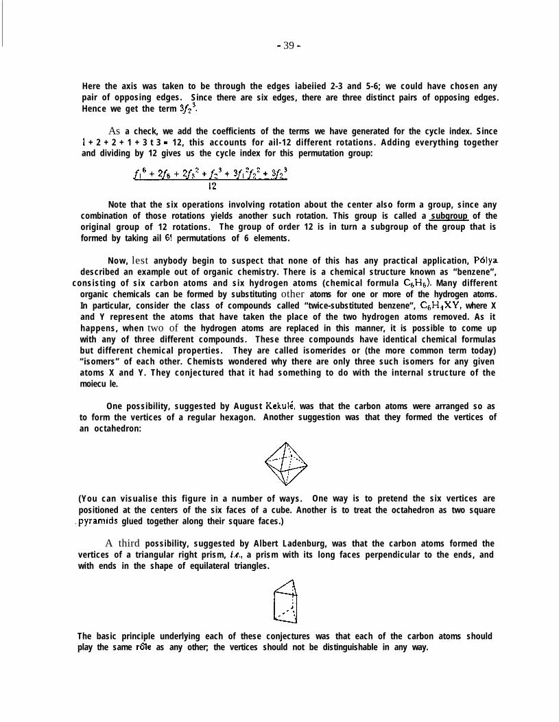
- 39 -

Here the axis was taken to be through the edges iabeiied 2-3 and 5-6; we could have chosen anypair of opposing edges. Since there are six edges, there are three distinct pairs of opposing edges.Hence we get the term 3f:?

As a check, we add the coefficients of the terms we have generated for the cycle index. Since1 + 2 + 2 + 1 + 3 t 3 = 12, this accounts for ail-12 different rotations. Adding everything togetherand dividing by 12 gives us the cycle index for this permutation group:

Note that the six operations involving rotation about the center also form a group, since anycombination of those rotations yields another such rotation. This group is called a subgroup of theoriginal group of 12 rotations. The group of order 12 is in turn a subgroup of the group that isformed by taking ail 6! permutations of 6 elements.

Now, lest anybody begin to suspect that none of this has any practical application, Poiyadescribed an example out of organic chemistry. There is a chemical structure known as “benzene”,

consisting of six carbon atoms and six hydrogen atoms (chemical formula C6H6). Many differentorganic chemicals can be formed by substituting other atoms for one or more of the hydrogen atoms.In particular, consider the class of compounds called “twice-substituted benzene”, C6H4XY, where Xand Y represent the atoms that have taken the place of the two hydrogen atoms removed. As ithappens, when two of the hydrogen atoms are replaced in this manner, it is possible to come upwith any of three different compounds. These three compounds have identical chemical formulasbut different chemical properties. They are called isomerides or (the more common term today)“isomers” of each other. Chemists wondered why there are only three such isomers for any givenatoms X and Y. They conjectured that it had something to do with the internal structure of themoiecu le.

One possibility, suggested by August Kekui6, was that the carbon atoms were arranged so asto form the vertices of a regular hexagon. Another suggestion was that they formed the vertices ofan octahedron:

(You can visualise this figure in a number of ways. One way is to pretend the six vertices arepositioned at the centers of the six faces of a cube. Another is to treat the octahedron as two square

-pyramids glued together along their square faces.)

A third possibility, suggested by Albert Ladenburg, was that the carbon atoms formed thevertices of a triangular right prism, i.e., a prism with its long faces perpendicular to the ends, andwith ends in the shape of equilateral triangles.

The basic principle underlying each of these conjectures was that each of the carbon atoms shouldplay the same r&e as any other; the vertices should not be distinguishable in any way.

- 40 -

How can we decide which model (if any) is right? We’ll represent the X atom by a dark circle(0) and Y by a light circle (0). How many different configurations are there? in each model, thecarbon atoms are indistinguishable, so it makes no difference where we attach the X atom. In how.many distinct ways can we attach the Y? For the hexagonal model, there are three ways.

0. 0The other two positions for the Y atom are the same as the first two, merely flipped over. Theoctahedral model has only two ways to place the Y atom.

The other three positions are identical to the first, except rotated about a vertical axis.

The third model is a bit trickier. No two of the five possible positions for the Y atom can berotated into each other without moving the X atom to a different position, so all five cases aredifferent.

The reason this case is tricky is that the last two cases are exact “mirror images” of the first two.That is, if you reflect the last two in a mirror, they will come out looking exactly like the first two.The question is, are mirror images chemically distinct? The answer is: they are. Two chemicalsthat are mirror images of each other will have slightly different chemical properties. (In fact, if yourbody were reflected like this on the molecular level, your reflected body would not be capable ofdigesting ordinary food! Your food would have to be specially prepared to consist of mirror-imageproteins and other reflected chemicals.)

So what have we established? If the carbon atoms were arranged as in an octahedron, therewould be only two possible isomers of C6H4XY. If they were arranged as in a triangular pr i sm ,there would be five isomers. In reality, chemists were able to find only three; therefore these twomodels are wrong. We haven’t actually proven that the hexagonal model is correct, but we havecircumstantial evidence in its favor. (Various other methods have backed this up, and modernchemists are essentially certain that the carbon atoms of benzene do indeed form a regular hexagon,at least insofar as chemical bonds maintain any rigid shape.)

This analysis, which enabled us to choose among the three available models, was fairly easy.Suppose it had been C6H2XY& or some other exotic set of compounds? The intent of this sectionis to come up with a mathematical method for doing this sort of analysis.

The preceding computation by which we arrived at the cycle index for the rotations of theregular hexagon, can be summarised by the following chart.

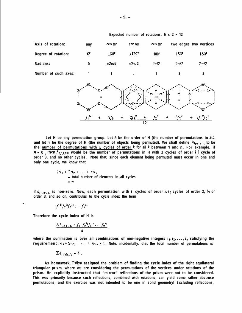
-4i-

Expected number of rotations: 6 x 2 = 12

Axis of rotation: any ten ter ten ter ten ter two edges two vertices

Degree of rotation: O0 k60° f 120° 180” 180’ 180’

Radians: 0 *2nl6 *2nl3 2nl2 2nl2 2nl2

Number of such axes: 1 1 1 1 3 3

fl 6 -I- 3 + 3f,2f22

12

Let H be any permutation group. Let h be the order of H (the number of permutations in H),and let n be the degree of H {the number of objects being permuted). We shall define hl,lziJ.,~l, to bethe number of permutations with ik cycles of order k for ail It between 1 and n. For example, ifn - 5 , then ~Z,O,I,O,O would be the number of permutations in H with 2 cycles of order 1, i cycle oforder 3, and no other cycles. Note that, since each element being permuted must occur in one andonly one cycle, we know that

i*i, + 2*i, + e l s + nd,= total number of elements in ail cycles=n

if hi,lT13,,,ln is non-zero. Now, each permutation with i, cycles of order 1, i2 cycles of order 2, is oforder 3, and so on, contributes to the cycle index the term

Therefore the cycle index of H is

where the summation is over ail combinations of non-negative integers i,, i:, . . . , i, satisfying ther e q u i r e m e n t i*ir + !2d2 + e 0 - + vi, = R. Note, incidentally, that the total number of permutations is

Ch =!I.t If:f?...f,

As homework, Wya assigned the problem of finding the cycle index of the right equilateraltriangular prism, where we are considering the permutations of the vertices under rotations of theprism. He explicitly instructed that “mirror” reflections of the prism were not to be considered.This was primarily because such reflections, combined with rotations, can yield some rather abstrusepermutations, and the exercise was not intended to be one in solid geometry! Excluding reflections,

- 42 -

we deduce that the group should be of order six, since there are six possible orientations for theprism. (We can choose any vertex to place at, say, the far left vertex of the upper face, and in sochoosing we establish the position of ail the other vertices as well. If mirror images were allowed, wewould still have the choice of whether or not to reflect the prism through a plane running throughthe upper-left vertex and the middle of the opposing face, so there would be twelve permutations.)There are two types of axes we need to worry about. One is the axis running vertically through thecenters of the two triangular faces. The others each rue horizontally through the center of a verticaledge and the center of the opposing face.

There are three such axes. Without further ado, here is the calculation of the cycle index forrotations of the prism.

Axis of rotation:

Degree of rotation:

Radians:

Number of such axes:

any

O0

0

--

Expected number of rotations: 6

vertical

*120”

*2nl3

1

edge/face

180”

2nl2

3

Just to see what we mean by “abstruse” rotations, let’s take a look at what happens if we includereflect the prismions in the permutation group. We can refiect across a horizontal plane (below left)or a vertical plane (below right). There are three such vertical planes, but only one permissible

6

horizontal plane {if the horizontal plane isn’t exactly midway between the two triangular faces, thereflection won’t cause the prism to coincide with itself), so we get four additional permutations. But’this gives us a total of only ten permutations, and we have already observed that there should betwelve. We cleverly deduce that we are missing two permutations, and after a bit of hunting wefind that we can combine a reflection with a rotation to yield a new permutation. Specifically, if wereflect the prism through the horizontal plane, we can then rotate it about the vertical axis. This isbest observed by numbering the vertices and watching what happens to them.

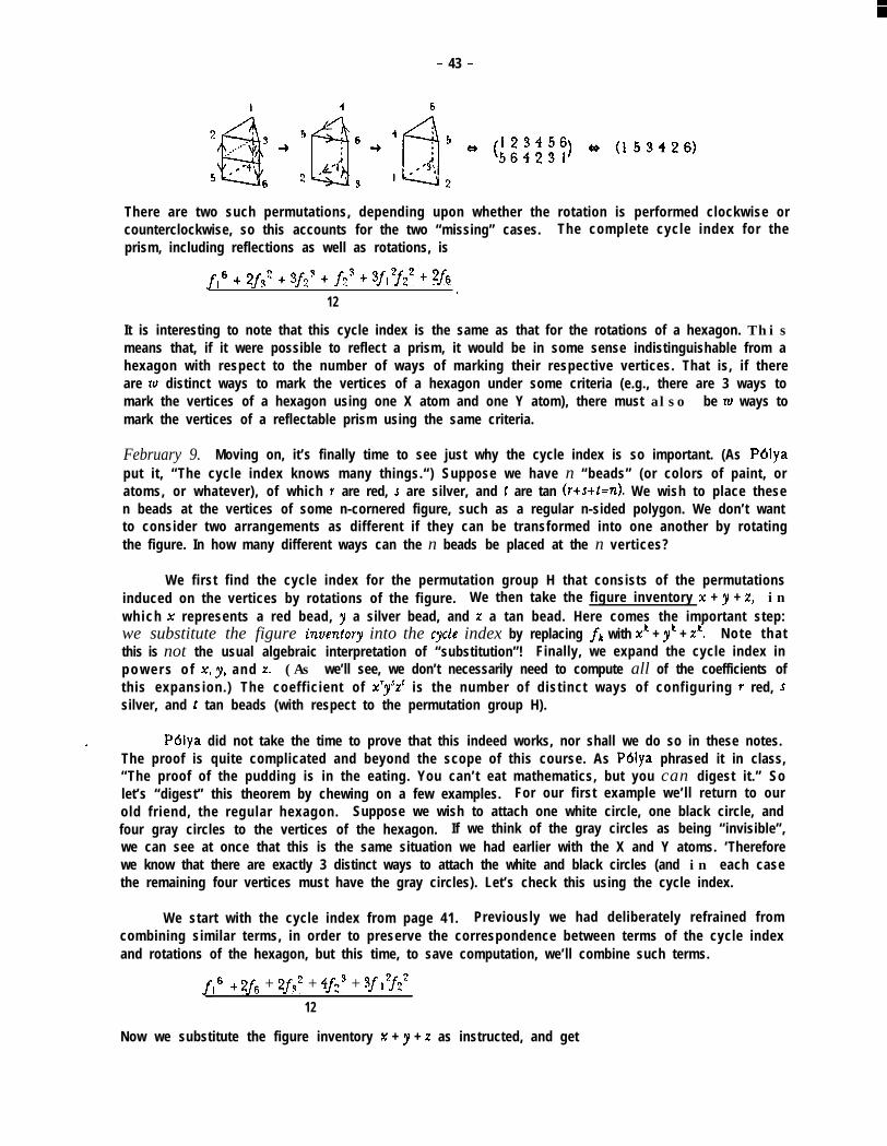
- 43 -

There are two such permutations, depending upon whether the rotation is performed clockwise orcounterclockwise, so this accounts for the two “missing” cases. The complete cycle index for theprism, including reflections as well as rotations, is

fl” + 2fy2 + 39 + fz3 + 3f12f2’ + 2f6.

12

It is interesting to note that this cycle index is the same as that for the rotations of a hexagon. Thismeans that, if it were possible to reflect a prism, it would be in some sense indistinguishable from ahexagon with respect to the number of ways of marking their respective vertices. That is, if thereare zu distinct ways to mark the vertices of a hexagon under some criteria (e.g., there are 3 ways tomark the vertices of a hexagon using one X atom and one Y atom), there must also be ru ways tomark the vertices of a reflectable prism using the same criteria.

February 9. Moving on, it’s finally time to see just why the cycle index is so important. (As P6iyaput it, “The cycle index knows many things.“) Suppose we have n “beads” (or colors of paint, oratoms, or whatever), of which Y are red, s are silver, and t are tan (rtstf=n). We wish to place thesen beads at the vertices of some n-cornered figure, such as a regular n-sided polygon. We don’t wantto consider two arrangements as different if they can be transformed into one another by rotatingthe figure. In how many different ways can the n beads be placed at the n vertices?

We first find the cycle index for the permutation group H that consists of the permutationsinduced on the vertices by rotations of the figure. We then take the figure inventory x + y + x, inwhich x represents a red bead, JI a silver bead, and z a tan bead. Here comes the important step:we substitute the figure inventory into the cycle index by replacing Jk with x’ + y’ + z! Note thatthis is not the usual algebraic interpretation of “substitution”! Finally, we expand the cycle index inp o w e r s o f 3c, y, and z. (As we’ll see, we don’t necessarily need to compute all of the coefficients ofthis expansion.) The coefficient of X’J’Z’ is the number of distinct ways of configuring r red, fsilver, and t tan beads (with respect to the permutation group H).

- P6iya did not take the time to prove that this indeed works, nor shall we do so in these notes.The proof is quite complicated and beyond the scope of this course. As P6iya phrased it in class,“The proof of the pudding is in the eating. You can’t eat mathematics, but you can digest it.” Solet’s “digest” this theorem by chewing on a few examples. For our first example we’ll return to ourold friend, the regular hexagon. Suppose we wish to attach one white circle, one black circle, andfour gray circles to the vertices of the hexagon. If we think of the gray circles as being “invisible”,we can see at once that this is the same situation we had earlier with the X and Y atoms. ‘Thereforewe know that there are exactly 3 distinct ways to attach the white and black circles (and in each casethe remaining four vertices must have the gray circles). Let’s check this using the cycle index.

We start with the cycle index from page 41. Previously we had deliberately refrained fromcombining similar terms, in order to preserve the correspondence between terms of the cycle indexand rotations of the hexagon, but this time, to save computation, we’ll combine such terms.

I 6 + 2y-s + 2fy2 + 4f2’ + 3f 12fz212

Now we substitute the figure inventory x + y + r as instructed, and get

- 44 -

(X+ytr)6 + 2(x6+y6tz6) + 2(x9+yJ+x")2 + 4(xz+y'+z')3 + 3(xtytz)‘(x~+y’+z~)~,12

Expanding this expression into powers of x, y, and x is not a tempting prospect. Fortunately, weneedn’t expand very much of it . Instead we can take advantage of an extension of the BinomialTheorem, to wit, the Muitinomiai Theorem (shown here for three variables-the generaiisation tomore than three variables should be obvious):

b+y+d” = ,+zrE, -$fyzr *. . .6!So, for example, the coefficient of #yz4 in (x+y+# is * which equals 30. 2(x6+$‘+z”) has. . .

no term of the form k*~yz~, nor does the third term, nor the fourth. The last term is

The only #J,z~ term coming out of that comes from 2xy*r4 which, multiplied by the outer coefficient3, gives a coefficient of 6. So the coefficient of J& in the expanded cycle index (with the figureinventory substituted in) is just 30 + 6 - 36. We now divide by the 12 and get a final answer of 3,which checks.

It was assigned as homework to use the cycle index of the prism to check the number of waysof placing one X atom and one Y atom thereon. We already know that the answer should be 5.Substituting the figure inventory into the cycle index shown on page 42, we get

(x+y+@ + 2(xJty"tzyt 3(x2+yw)3 .6

Once again we’re looking for the coefficient of #yz4. The first term yields a coefficient of 30 asbefore, and the other two expansions yield no xyz4 terms. So the coefficient of xyzJ in the expandedcycle index is 30, which when divided by 6 gives the expected answer, 5.

Another example: suppose we have three colors of paint, and we wish to paint the corners ofan equilateral triangle. In how many ways can we do this? First, we find the cycle index. We,computed this back on page 36, so we won’t do it here. We substitute the figure inventory x + y + 2,representing the three different colors of paint, into the cycle index to get

(x+y+z)" + 3(x+y+z)(x~+~~+z') + 2(xJ+yY+zY)6

This time we haven’t specified which combination of colors we’re interested in, so we’d bestcompute ail the coefficients in the expansion. Even so, it’s not as difficult as it looks, because theexpression is symmetric with respect to x, y, and z. Thus it suffices to look at the coefficients of x3,x’J,, and xyz. Every other term is symmetrically equivalent to one of these; for instance, ~‘2 has thesame coefficient as x2y. So we proceed to fill out a little table showing the coefficients of the threedifferent kinds of terms in each part of the expansion.

x3 v(xtg+r)s 3!.j L-3 3!=6

3!0!0! 2! 1 !O! l!i!i!

3(x+y+z)(x2yZ+z2) 3 3 0

2 0 0

- 450

Adding up each column and dividing through by 6, we find that every coefficient is I. It’s time foranother of Polya’s maxims: "if you see a fact, try to see it as intuitively as possible.” What does itmean for every coefficient to be l? It means that each combination of colors can be applied inexactly one way. We’ll see later why this should be the case.

.

The n! possible permutations of n elements form a group, since if you reorder n objects once,and then reorder them again, you get yet another ordering. This group has degree n and order n!,and is called the symmetric group. We shall denote it by S,. Let’s try to find the cycle index of thisgroup.

February 14. Consider any single permutation. Suppose it has i, cycles of order 1, i2 of order2 * * I andn-&t be

i, of order n. The total number of elements in these cycles, as we’ve observed before,

14, + 2*i2 + e - a + nei, = n .

What is 4,/*13..ffl 3 (The following proof is due to Cauchy.) We consider any permutation, broken upinto its component cycles. First we show the cycles of order I, representing each by a square.

We then show the cycles of order 2, representing each by two squares.

mm.,,[-IWe carry on in this fashion until we’ve shown all the cycles.

4.12 i3 i, (= 0 or 1)

oo...o m... im..: .a. rrrmTl

Having put the permutation into this form, we note that there must be exactly n s q u a r e sinvolved. So we proceed to write any permutation of th~Qn~u~r$~r;,l to n inside the squares. Forinstance, suppose n = 9, and start with the permutation (., ; 9, 26 s 5 5). In the cycle notation this is(6)(1 4)(3 9)(2 7 8 5) so our “square” drawing looks like this:

nmmr .We then take an arbitrary permutation of the numbers I through 9 and plunk the numbers into thesquares. For instance, let’s use the permutation: 5 9 1 2 7 4 3 6 8.

If we inter-fret this as a collection of cycles, we get (5)(9 I)(2 ‘1)(4 3 6 8), which can also be written as( i p i “1 :z i ,, y). In other words, by taking various permutations of the integers 1 through n andplacing them in the squares, we can obtain a mapping from those permutations onto the set of

- 46 -

permutations with this particular cycle form. Of course, more than one permutation, when placed inthe squares, may yield the same result. For example, consider the permutation: 5 7 2 9 1 8 4 3 6.Placed in the squares, this produces

which is again the permutation ((I, 6 s 58 :, ,’ ’ s 4 5 6 ‘8 a). Consider any permutation P with this cycle form. Ifwe plug each of the n! permutations into the squares, how many times do we produce PI If P has iicycles of order 1, then in order to produce P the i, elements contained in those cycles must be placedin the il squares representing cycles of order 1. However, they can be placed in any order withinthose squares, so there are i,! ways to do it. Meanwhile, if P has iT cycles of order 2, then toproduce P the iz pairs of elements in those cycles have to be placed in the iT pairs of squaresrepresenting cycles of order 2. The pairs may be placed in any of 1%.7 orders, and furthermore eachpair can be rotated; that is, the cycle (a b) can also be written (b a). Since there are i, cycles, each ofwhich can be rotated into either of two forms, we get a factor of 2**. In general, suppose P has ikcycles of order k. Then these cycles can be arranrotated into any of k forms, so we get a factor of ik.k H

ed in any of ik! ways, and each cycle can be1 h. Altogether, therefore, there are

i,!l’l 6 i2!2’2 l i9!313 l , , , l i,!n’”.

permutations that, when placed in the squares, yield the cycles of P. If we plug every one of the n!possible permutations into the squares, each permutation with this particular cycle form is generatedexactly that many times. But we “know” how many permutations have this form; at least, we’vegiven it a name. So we conclude that

4 ,f*f ?...f, l i,!l�l l i2!2’? l i9!3f3 * , , , l i,!nfn 0 n!

and that the cycle index of the symmetric group S, is therefore

- $1 c n!i,!P ’l i2!P 0 t11.3* I i3 ,

. . . l i,!nln f,‘pf~‘3 . . t fn’“.

Recall that this summation is over all values of the i’s such that 14, + 24, + l l - + vi, - n. Thereis-a trick we can use to find all such values. We observe that

In other words, each set of values for i, through i, corresponds to a unique way of representing thenumber n as a sum of positive integers. So if we look at all sets of positive integers that sum to n,we can compute from them all possible values for the I’s

Let ’s see how th is works by look ing a t the case n - 3. We can write 3 as 1+ 1+1, w h i c hcorresponds to the case i, - 3, i2 - 0, is - 0. We can also write 3 as 1+2, or we could simply write itas 3. These cases are tabulated on the following page.

3

- 47 -

cycle form cycle index coefficient

311+1+1

3=1+2

3=3

f?

0 flf2

f.9

3! P 13!1”

3! -3z-i$

3! 2iiT

(We’ve omitted factors of O!k" from the denominators in the last column.) So the cycle index of S3 is

This should look familiar-it’s the cycle index for rotations of a triangle. This explains whythere’s only one way to paint the vertices of a triangle with any given set of colors; if we try to applythe same colors to the vertices in some other order, we can always permute the vertices back to thefirst order, because no matter what the rotation is it must be in the symmetric group.

What about St? Does its cycle index correspond to anything tangible, such as rotations of asquare or tetrahedron? Well, yes, but it’s neither of those. The square has 8 rotations, while thetetrahedron has 12: The symmetric group, on the other hand, has 4! = 24 permutations, so it can’tcorrespond to either of those figures. Let’s work it out and see what it looks like. We must firstfind all possible ways of representing 4 as a sum of positive integers. If the positive integers includea 1, then the remaining integers sum to 3, and we already know there are three cases. If the.positiveintegers do not include a 1, then we can have 2-t-2, or simply 4. Here we go then with another table:

4 i2 i3 i4 cycle form cycle index coefficient

4=1+1+1+1 4

4=1+1+2 2 1

f14

0 f fI2 2

4! 14!14=

4! 62!1'1!21-

4=1+3 1 0 1 0 ff I 3 4! 4i7i-m

4=2+2 0 2 0 0 fz2 4! cl32!2"

4=4 0 0 0 1 f4 4! 6iT=

i As a check, the coefficients should sum to 4!. 1 + 6 + 8 + 3 + 6 - 24 = 4!. So S4 has the cycle index

I 4 + 6f12f2 t 8f ,fs + 3fc2 t 6f4.

24

It turns out this is the cycle index for rotations of the diagonals of a cube, as was discoveredon the midterm. {We’ll have more to say about this in the solution to the midterm, which is insection 8.)

Now we come to the grand finale for this section, but don’t hold your breath-it’s a l o n gfinale! So far we’ve only considered figure inventories of a rather limited form: the sum of distinctvariables. When we had k possible choices from which to pick a “value” to be assigned to each ofthe elements being permuted, we associated a unique variable with each choice and took the figure

- 48 -

inventory to be the sum of those variables. For example, if we were coloring the vertices of thetriangle using three colors, we associated each color with a variable and took the sum: x + y + z.There is a more general form of the figure inventory, which we shall now examine.

The basic idea is that we associate with each choice a value that is not necessarily a uniquevariable. One of the suggested references ([Liu], pages 145-146) has a good example that introducesthis concept; it is presented here with the permission of the author. Suppose you have three ballsyou wish to paint. You have three types of paint available- a cheap red paint, an expensive redpaint, and a blue paint. In how many ways can you paint the balls? We wish to count as differentthe cases where the same paints are used but in different orders; that is, the case where the first twoballs are painted blue and the last one cheap red is to be counted separately from the case where thefirst ball is painted cheap red and the other two blue, and so forth. Hence we are not allowing anypermutations other than the identity permutation, and the cycle index is simply f I !

We can represent the three kinds of paint by three variables, rl (expensive red), r2 (cheapred), and b (blue). The figure inventory is rl t y2 + b. Substituting this into the cycle index yields

(Y, + r2 + b)’ = Y,' + r2’ + b” + 3~,~y~ t ~Y,Y~~ t 3~,~b + 3y2’b t 3y,b2 + 3y,b2 + 6r,y2b.

Thus, for instance, the term 3rlrz2 means that there are three ways to paint the balls using theexpensive red paint on one ball and the cheap red paint on the other two. Suppose, however, thatwe were to represent both the cheap red paint and the expensive red paint by the same variable, Y.It is clear that the coefficient of, say, y’b, will be the sum of the coefficients of y,‘b, yly2b, and y22b.In other words, the coefficient of y2b will be the number of ways of painting the balls using a n ycombination of the red paints on two balls and blue paint on the remaining ball.

(Y + Y + b)> = (2~ t b)’ = 8~’ t 12r2b t 6rb2 + b”

We observe, for example, that there are 8 ways to paint all three balls red. This makes sense, sincefor each ball we can choose either of the two red paints.

Let’s take a closer look at what we’ve just done. Instead of saying that we had three kinds ofpaint, we said we had only two kinds, but that there were two paints of the first kind and one of thesecond. If we had had five kinds of red paint, three kinds of blue paint, and two kinds of greenpaint, we would have used the figure inventory 5~ t 36 t 2g, We can generalise this stil l further.Suppose we wish to place colored beads at the vertices of a regular hexagon. Each bead can be anyof three colors, but there are different kinds of beads for each color. For instance, there may beround red beads, cubical red beads, and elongated red beads, and similarly let us suppose there arethree kinds of blue beads and three kinds of green beads. Then we would use the fi3r + 36 + 3g. If we were to substitute this into the cycle index, the coefficient of y’b!g H

ure inventorywould be the

number of ways of placing i red beads, j blue beads, and k green beads on the vertices of thehexagon, where two ways are considered different if they use differently shaped beads. This isessentially the same sort of thing as what we did with the different kinds of paint in the previousexample. Now for that next step: Suppose, for simplicity, that there is only one shape for each colorof bead, but that we are placing chters of beads at each vertex. We’ll assume each cluster must beone of a finite number of possibilities. For instance, we can place two red beads and a blue beadtogether at a vertex, or we can place three green beads, or we can place a blue bead and a greenbead. No other combinations are allowed. Then we shall represent this by the figure inventoryy2b + g’ + bg. If we substitute this figure inventory into the cycle index, the resulting coefficient ofr’b’g’ is the number of distinct ways of placing clusters of beads such that exactly i red beads, j bluebeads, and k green beads are used.

The general form of the figure inventory is defined to be

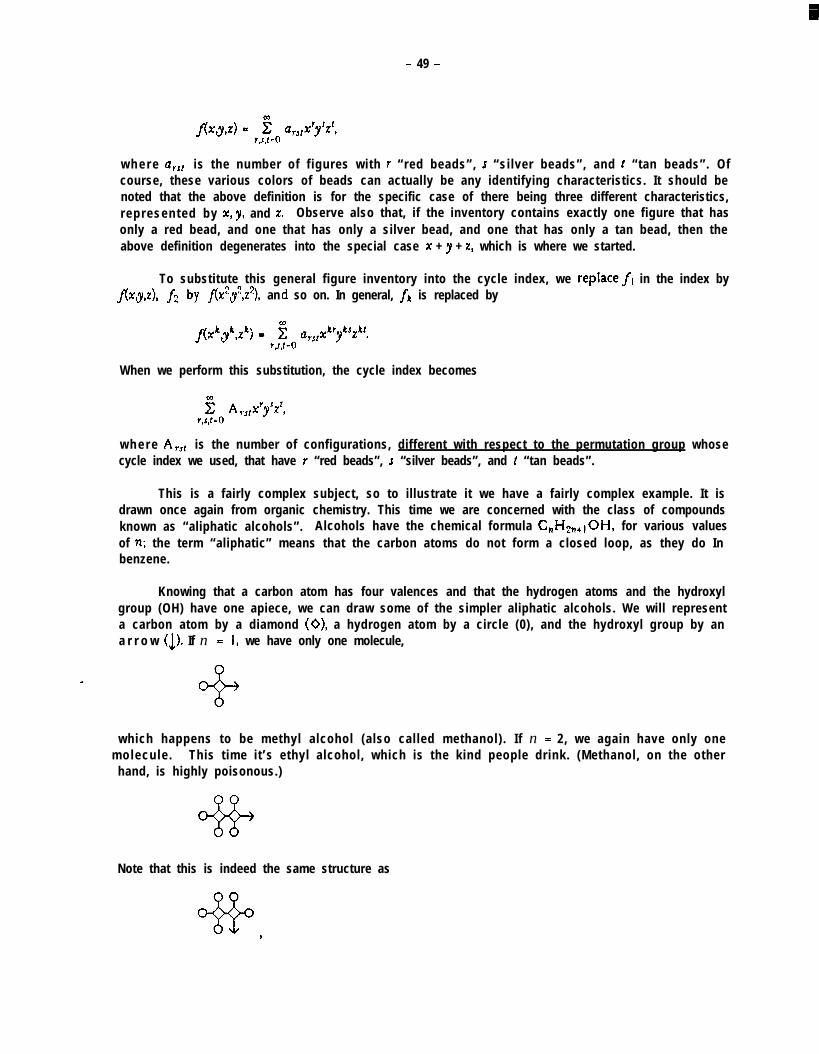
- 49 -

w h e r e a,,, is the number of f igures with Y “red beads”, J “silver beads”, and t “tan beads”. Ofcourse, these various colors of beads can actually be any identifying characteristics. It should benoted that the above definition is for the specific case of there being three different characteristics,represented by x, y, and x. Observe also that, if the inventory contains exactly one figure that hasonly a red bead, and one that has only a silver bead, and one that has only a tan bead, then theabove definition degenerates into the special case x + y + z, which is where we started.

To substitute this general figure inventory into the cycle index, we replaceft in the index byfky,dt f2 by f(x2,y2d, and so on. In general, fk is replaced by

When we perform this substitution, the cycle index becomes

w h e r e ArJt is the number of configurations, different with respect to the permutation group whosecycle index we used, that have Y “red beads”, J “silver beads”, and t “tan beads”.

This is a fairly complex subject, so to illustrate it we have a fairly complex example. It isdrawn once again from organic chemistry. This time we are concerned with the class of compoundsknown as “aliphatic alcohols”. Alcohols have the chemical formula CnH2,+r0H, for various valuesof n; the term “aliphatic” means that the carbon atoms do not form a closed loop, as they do Inbenzene.

Knowing that a carbon atom has four valences and that the hydrogen atoms and the hydroxylgroup (OH) have one apiece, we can draw some of the simpler aliphatic alcohols. We will representa carbon atom by a diamond (0)) a hydrogen atom by a circle (0), and the hydroxyl group by ana r r o w (1>. If n = 1, we have only one molecule,

which happens to be methyl alcohol (also called methanol). I f n = 2, we again have only onemolecule . This time it’s ethyl alcohol, which is the kind people drink. (Methanol, on the other

hand, is highly poisonous.)

Note that this is indeed the same structure as

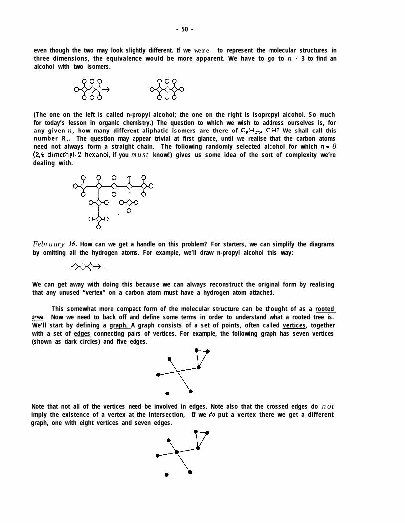
- 50 -

even though the two may look slightly different. If we were to represent the molecular structures inthree dimensions, the equivalence would be more apparent. We have to go to n = 3 to find analcohol with two isomers.

(The one on the left is called n-propyl alcohol; the one on the right is isopropyl alcohol. So muchfor today’s lesson in organic chemistry.) The question to which we wish to address ourselves is, forany g iven n, how many different aliphatic isomers are there of C,Hz,+lOH? We shall call thisn u m b e r R , . The question may appear trivial at first glance, until we realise that the carbon atomsneed not always form a straight chain. The following randomly selected alcohol for which n - 8(2,4-dimethyl-2-hexanol, if you must know!) gives us some idea of the sort of complexity we’redealing with.

February lb. How can we get a handle on this problem? For starters, we can simplify the diagramsby omitting all the hydrogen atoms. For example, we’ll draw n-propyl alcohol this way:

We can get away with doing this because we can always reconstruct the original form by realisingthat any unused “vertex” on a carbon atom must have a hydrogen atom attached.

This somewhat more compact form of the molecular structure can be thought of as a rootedtree2 Now we need to back off and define some terms in order to understand what a rooted tree is.We’ll start by defining a graph. A graph consists of a set of points, often called vertices, togetherwith a set of edges connecting pairs of vertices. For example, the following graph has seven vertices(shown as dark circles) and five edges.

Note that not all of the vertices need be involved in edges. Note also that the crossed edges do notimply the existence of a vertex at the intersection, If we do put a vertex there we get a differentgraph, one with eight vertices and seven edges.

- 51 -

A sequence of edges forming a closed loop, such as the triangle in the preceding graphs, iscalled a circuit. A graph is said to be connected if it is possible to get from any vertex to everyother vertex by following the edges. Neither of the preceding graphs is connected, because there isno way to get to the isolated vertex from any other vertex. A graph that is connected and that has’no circuits is called a tree. Of the three graphs shown below, only the rightmost one is a tree. (Theleftmost one isn’t connected, whereas the center one has a circuit.)

One noteworthy feature of trees, which you might try proving, is that in any tree the numberof vertices is one greater than the number of edges. In a tree, an “endpoint” (that is, a vertex withonly one edge) is called a leaf. In general, the number of edges entering a vertex is called the orderor degree of that vertex. Thus the tree shown above has one vertex of degree 3, four of degree 2,and three of degree 1. (These last three are therefore leaves.) If one of the vertices in a tree isdistinguished from the others in some manner (e.g., by marking it with an arrow), that vertex iscalled the root of thg tree, and the tree is called a rooted tree.

Now that we’ve defined what we mean by a rooted tree, let’s get back to chemistry. In analiphatic alcohol, the carbon atoms must certainly be connected; otherwise we’d have two smallermolecules. Furthermore, by the definition of the term “aliphatic”, there can be no closed loops.Hence the carbon atoms form a tree. We’ll let the carbon atom that is connected to the hydroxylgroup (OH) be the root of the tree. We observe that no carbon atom can be bonded to more thanfour other carbon atoms (or four of any kind of atoms, for that matter), and that the root can beconnected to at most three other carbon atoms, since one of its valences is being used to bond withthe hydroxyl group. This means that the carbon atoms form a rooted tree in which each vertex hasdegree < 4 and the root has degree < 3. Conversely, any rooted tree meeting these criteria regardingthe degrees of the vertices corresponds to a unique aliphatic alcohol. We have therefore succeededin transforming our chemical problem into the mathematical one of determining the number of suchrooted trees with a given number of vertices.

Chemists solved this problem by trial and error for some small values of n. Our job is tofind the solution mathematically. As usual, we’ll start by inspecting the simplest cases and lookingfor a pattern. We can create all the trees with n vertices by taking each tree with n-l vertices andattaching another vertex in all possible ways. (Some n-vertex ,trees may be generated more thanonce, in which case we’ll eliminate the duplicates.)

n 1

P

Rn 1

2

8

1

3

I42

There’s no immediately obvious pattern. We might guess that R, is always a power of two, but we’dbe wrong. As it turns out, R5 noes happen to be 8, but R6 is 17. Though it’s always a good idea tolook for a pattern, patterns can sometimes be deceiving!

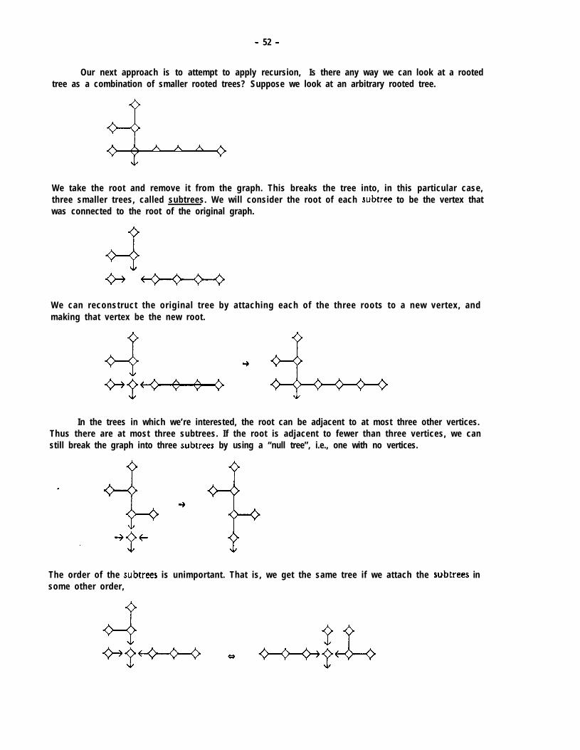
- 52 -

Our next approach is to attempt to apply recursion, Is there any way we can look at a rootedtree as a combination of smaller rooted trees? Suppose we look at an arbitrary rooted tree.

A A A

We take the root and remove it from the graph. This breaks the tree into, in this particular case,three smaller trees, called subtrees. We will consider the root of each subtree to be the vertex thatwas connected to the root of the original graph.

We can reconstruct the original tree by attaching each of the three roots to a new vertex, andmaking that vertex be the new root.

In the trees in which we’re interested, the root can be adjacent to at most three other vertices.Thus there are at most three subtrees. If the root is adjacent to fewer than three vertices, we canstill break the graph into three subtrees by using a “null tree”, i.e., one with no vertices.

The order of the subtrees is unimportant. That is, we get the same tree if we attach the subtrees insome other order,

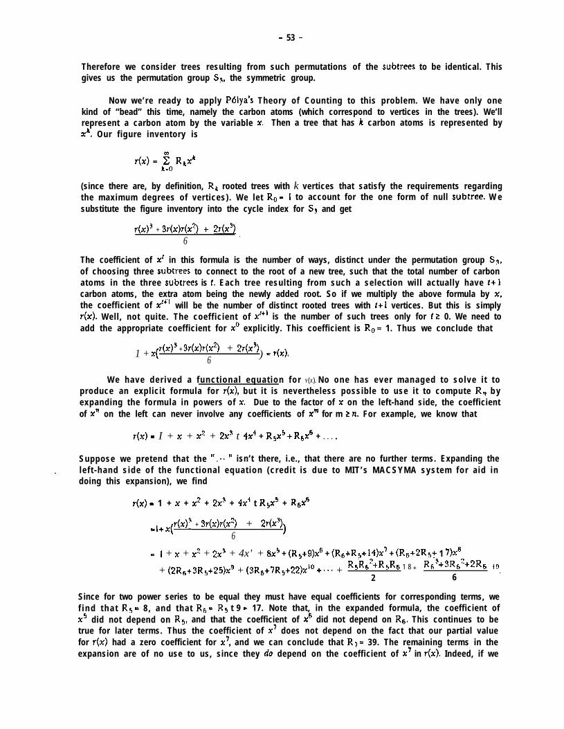
- 53 -

Therefore we consider trees resulting from such permutations of the subtrees to be identical. Thisgives us the permutation group Sy, the symmetric group.

Now we’re ready to apply Pblya’s Theory of Counting to this problem. We have only onekind of “bead” this time, namely the carbon atoms (which correspond to vertices in the trees). We’llrepresent a carbon atom by the variable X. Then a tree that has k carbon atoms is represented byxk. Our figure inventory is

(since there are, by definition, Rh rooted trees with k vertices that satisfy the requirements regardingthe maximum degrees of vertices). We let R0 - I to account for the one form of null subtree. W esubstitute the figure inventory into the cycle index for S3 and get

Y(# + 3r(x)r(x4 + 2r(x3) .6

The coefficient of x’ in this formula is the number of ways, distinct under the permutation group Ss,of choosing three subtrees to connect to the root of a new tree, such that the total number of carbonatoms in the three subtrees is t. Each tree resulting from such a selection will actually have t+lcarbon atoms, the extra atom being the newly added root. So if we multiply the above formula by 3c,the coefficient of xii’ will be the number of distinct rooted trees with 1t I vertices. But this is simplyY(X). Well, not quite. The coefficient of x’+’ is the number of such trees only for t L 0. We need toadd the appropriate coefficient for x0 explicitly. This coefficient is R. = 1. Thus we conclude that

1 + x( Y($ + 3r(x)r(x2) + 2r(x96 ) = y(x).

We have der ived a funct iona l equat ion for Y(X). No one has ever managed to solve i t toproduce an explicit formula for Y(X), but it is nevertheless possible to use it to compute R, b yexpanding the formula in powers of X. Due to the factor of x on the left-hand side, the coefficientof x” on the left can never involve any coefficients of x”’ for m 2 tl. For example, we know that

Y(X) = I + x + x2 + 2x3 t 4x4 + Rsx5 + Rsx6 + l l l .

Suppose we pretend that the ” l e n ” isn’t there, i.e., that there are no further terms. Expanding the- le f t -hand s ide of the funct ional equat ion (credi t is due to MIT’s MACSYMA system for a id in

doing this expansion), we find

Y(X) = 1 + x + x2 + 2x” + 4x4 t R5x5 + R6x”

- 1 + x(Y(Y)3 + 3r(x)r(x2) + 2r(x")6 1

e 1 + x + x2 + 2x' + 4x' + 8x5 + (R5t9)X6 + (R6+R5+ 14)x’ + (R6+2R5+ 1 7)X8

+ (2R6t3R5+25)#' + (3&j+7R5+22)d0 + * * * + R5R62+R5R6 1 8 + R63+3R62+2R6 ICJl

2 6

Since for two power series to be equal they must have equal coefficients for corresponding terms, wef i n d t h a t R!, = 8 , and that R6 = R5 t 9 = 17. Note that, in the expanded formula, the coefficient ofx5 did not depend on R5, and that the coefficient of x6 did not depend on R6. This continues to betrue for later terms. Thus the coefficient of X’ does not depend on the fact that our partial valuefor Y(X) had a zero coefficient for x7, and we can conclude that R7 = 39. The remaining terms in theexpansion are of no use to us, since they clo depend on the coefficient of x7 in Y(X). Indeed, if we

- 54 -

were doing th is by hand (MACSYMA, in case you don’ t recognise the name, is a computerisedsystem for doing sophisticated symbolic mathematical manipulations), we wouldn’t have botheredcomputing any terms beyond X? Having found R5, R6, and RT, we could extend our partial powerseries for Y(X), re-expand the functional equation, and evaluate a few more coefficients.

That’s all we have to say about Pblya’s Theory of Counting. For further reading, just aboutany good book on combinatorics will suffice, though most make use of rather complex mathematicalnotations. Chapter 5 of [Liul is probably as good as-any other. The analysis involving aliphaticalcohols is included in the December, 1956, issue of the American Mathematical Monthly. For theavid reader, chapters 4 and 5 of (Balaban] discuss methods, including P6lya’s theory, for countingvarious acyclic and cyclic chemical compounds, including unsubstituted alkanes (&Hz,+? as opposedto C&H 2n+10H), stereo-isomers (in which mirror images are counted as distinct molecules), and othercomplex structures.

cl7 Outlook

Everything we’ve been doing in the preceding sections has been counting combinatorics, that is,combinatorics in which we compute the number of configurations meeting certain criteria. Suchproblems make up one branch of combinatorics; there are two other classes of problems on which wehaven’t even touched. In this section we take a brief look at these other branches of combinatorics.Some of the subjects introduced here will be covered in greater depth by Tarjan in later sections.

One of the other branches is existential combinatorics. In existential problems we no longerwish to count anything; we just want to know whether any configuration exists meeting certaincriteria. For example, suppose there are n people at a party. We’ll assume n is at least 2 (otherwiseit’s not much of a party). Some people are acquainted with others, where “being acquainted” is amutual relationship. That is, if a person x is acquainted with another person y, then y is likewiseacquainted with X. Then we claim that Jome true people at the party have exactly the same numberof acquaintances at the party. We don’t know who the two people are; we don’t know how manyacquaintances they have; we don’t know whether there are more than two people with the samenumber of acquaintances. But we claim that some two people have the same number. This sort ofclaim is in the domain of existential combinatorics.

s The preceding claim is easy enough to prove. Each person at the party has some number ofacquaintances. No person can have fewer than zero acquaintances, and no person can have morethan n-l acquaintances. (We’re assuming the relationship of “acquaintance with” does not apply tooneself. If we instead assume that everyone is acquainted with himself, it just adds 1 to eachperson’s number of acquaintances, and so does not affect the result.) Therefore there are exactly npossibilities for the number of acquaintances a person has. Suppose the claim is wrong; suppose notwo of the n people have the same number of acquaintances. Then there must be exactly oneperson with no acquaintances, one with one acquaintance, one with two,. . . , and one with n - iacquaintances. This person who has n-l acquaintances must be acquainted with each of the othern-l people. But one of those people is supposed to have no acquaintances. This is a contradiction;hence the claim must be correct.

The third branch of combinatorics is called constructive combinatorics. This area deals withproblems where we don’t care how many configurations exist meeting some criterion, nor whetherthey exist (usually it’s obvious from the statement of the problem that some configuration exists), butrather we wish tofinn one such configuration. For example, suppose you own a number of shops inSan Francisco. Each shop is run by one employee, who lives somewhere in the city. There are

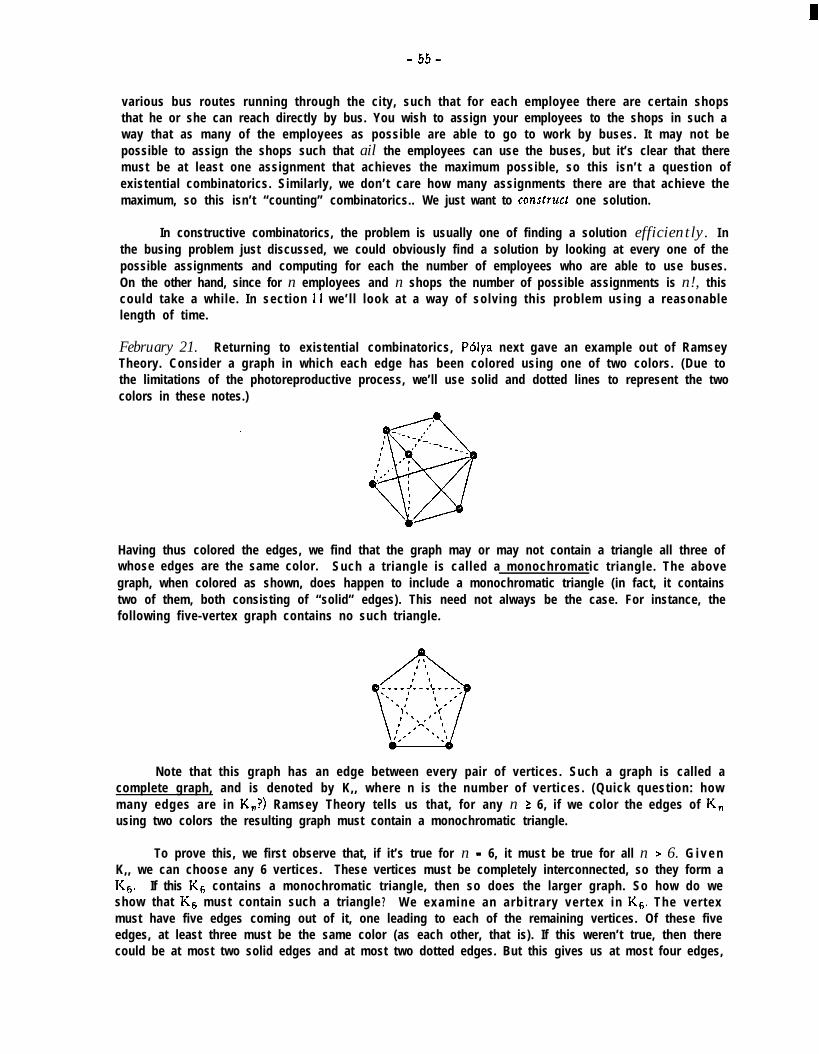
- 55-

various bus routes running through the city, such that for each employee there are certain shopsthat he or she can reach directly by bus. You wish to assign your employees to the shops in such away that as many of the employees as possible are able to go to work by buses. It may not bepossible to assign the shops such that ail the employees can use the buses, but it’s clear that theremust be at least one assignment that achieves the maximum possible, so this isn’t a question ofexistential combinatorics. Similarly, we don’t care how many assignments there are that achieve themaximum, so this isn’t “counting” combinatorics.. We just want to con~tru.ct one solution.

In constructive combinatorics, the problem is usually one of finding a solution efficiently. I nthe busing problem just discussed, we could obviously find a solution by looking at every one of thepossible assignments and computing for each the number of employees who are able to use buses.On the other hand, since for n employees and n shops the number of possible assignments is n!, thiscould take a while. In section 11 we’ll look at a way of solving this problem using a reasonablelength of time.

February 21. Returning to existential combinatorics, P6lya next gave an example out of RamseyTheory. Consider a graph in which each edge has been colored using one of two colors. (Due tothe limitations of the photoreproductive process, we’ll use solid and dotted lines to represent the twocolors in these notes.)

--

Having thus colored the edges, we find that the graph may or may not contain a triangle all three ofwhose edges are the same color. Such a triangle is called a monochromatic triangle. The abovegraph, when colored as shown, does happen to include a monochromatic triangle (in fact, it containstwo of them, both consisting of “solid” edges). This need not always be the case. For instance, thefollowing five-vertex graph contains no such triangle.

Note that this graph has an edge between every pair of vertices. Such a graph is called acomplete graph, and is denoted by K,, where n is the number of vertices. (Quick question: howmany edges are in K,?) Ramsey Theory tells us that, for any n L 6, if we color the edges of K,using two colors the resulting graph must contain a monochromatic triangle.

To prove this, we first observe that, if it’s true for n = 6, it must be true for all n > 6. G i v e nK,, we can choose any 6 vertices. These vertices must be completely interconnected, so they form aI&. If this KG contains a monochromatic triangle, then so does the larger graph. So how do weshow that K6 must contain such a triangle ? We examine an arb i t rary ver tex in K6. The vertexmust have five edges coming out of it, one leading to each of the remaining vertices. Of these fiveedges, at least three must be the same color (as each other, that is). If this weren’t true, then therecould be at most two solid edges and at most two dotted edges. But this gives us at most four edges,

- 56 -

and there are supposed to be five. So we have either three solid edges or three dotted edges. (Wecould have more than three, but we don’t care about that.) Without loss of generality, let’s assumethe three edges are all solid.

0

Now consider the three vertices at the “other ends” of those edges. There must be edgesbetween every pair of vertices, since this is a complete graph. If any two of these three vertices areconnected by a solid edge, we’ve got a solid triangle. If no two of the three are connected by a solidedge, then they must be connected by dotted edges, and we’ve got a dotted triangle as shown below.

Notice that a triangle is simply a complete graph with three vertices. Suppose we wished toprove that, for some sufficiently large n, I<, cannot be colored with two colors wrthout producing amonochromatic IL,? It’s not too difficult to prove that, for any J, there is some number n sufficientlyl a r g e t h a t K, must, if colored with two colors, contain a monochromatic I<,. Unfortunately, nogeneral method is known for finding that number! We’ll look at this and related problems insection 9.

Existential combinatorics need not always deal with conclusions of the form, “Such-and-suchexists.” Sometimes the result can be probabilistic. For example, Erd6s has proved several resultsinvolving randomly-generated graphs. We won’t attempt to prove any of these results here, but willsimply mention one such result as an example of this sort of problem. Suppose you generate agraph by the following method. You start with n vertices and no edges. You then repeatedly pickany two vertices that are not yet joined by an edge, and add that edge to the graph. Your selectionof which edge to add each time is completely random; any edge not yet in the graph is as likely to bechosen as any other edge. Stop adding edges as soon as you add an edge that makes the graphconnected (as defined on page 51). How many edges are in the graph? Obviously, the number ofedges ‘wil l vary depending on the order in which you choose to add them to the graph; if youhappen never to choose an edge involving some particular vertex (until, of course, there are noother edges from which to choose), then there will be many edges indeed. On the other hand, thegraph could be connected after as few as n-l edges have been chosen (in which case the graphwould be a tree). Erdas has proved that, for any constant Iz, the probability that the graph hasfewer than kn+bzlog,n edges approaches em*-’ as n goes to infinity.

This result may sound rather far-fetched, but it has some simple corollaries. For instance, ifyou select a graph at random from among those with n vertices and d5 edges, where n is fairlylarge, the graph will almost certainly be connected. This is because d5 is, for sufficiently large n ,greater than kn+hlog,n for any constant le. So we can let k=lOO (for instance) and deduce that theprobability is roughly e-“-“I’ x 1 that lOOn+hlog,n edges are enough to connect the graph, and n’*5

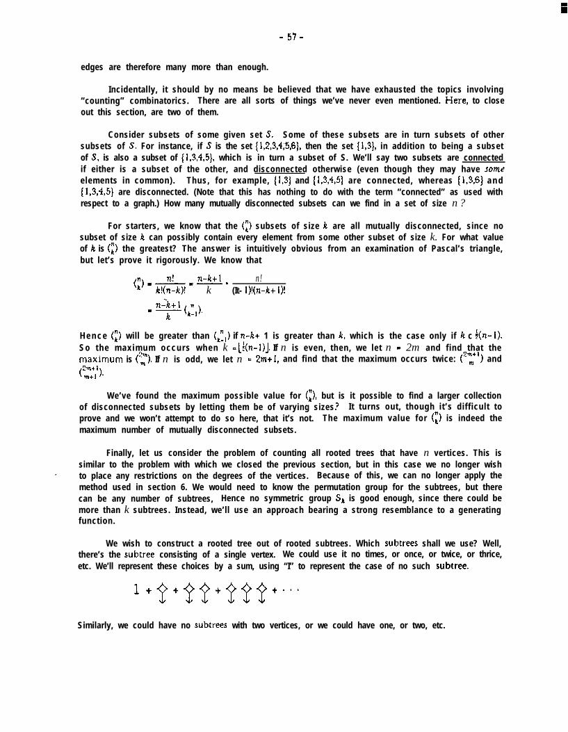
- 57-

edges are therefore many more than enough.

Incidentally, it should by no means be believed that we have exhausted the topics involving“counting” combinatorics. There are all sorts of things we’ve never even mentioned. H,ere, to closeout this section, are two of them.

Consider subsets of some given set S. Some of these subsets are in turn subsets of othersubsets of S. For instance, if S is the set { 1,2,3,4;5,6], then the set {1,3j, in addition to being a subsetof S, is also a subset of (1,3,4,5), which is in turn a subset of S. We’ll say two subsets are connectedif either is a subset of the other, and disconnected otherwise (even though they may have ~07neelements in common). Thus, for example, (i,3j and {1,3,4,5) are connected, whereas (1,3,6) a n d(1,3,4,5) are disconnected. (Note that this has nothing to do with the term “connected” as used withrespect to a graph.) How many mutually disconnected subsets can we find in a set of size n ?

For starters, we know that the (z) subsets of size k are all mutually disconnected, since nosubset of size k can possibly contain every element from some other subset of size k. For what valueof k is (z) the greatest? The answer is intuitively obvious from an examination of Pascal’s triangle,but let’s prove it rigorously. We know that

n-k+ 1(i) = n! ‘= - * n!It!(n-k)! k (It- i)!(n-)tt i)!

H e n c e (l) will be greater than (,1,) if n-ltt 1 is greater than k, which is the case only if K c f(n-1).So the maximum occurs when k - [!(n-i)j. If n is even, then, we let n = 2m and find that thema.ximum is (T). If n is odd, we let n - 2mti, and find that the maximum occurs twice: (2”,+1) and

(C,i’ ,.

We’ve found the maximum possible value for (i), but is it possible to find a larger collectionof disconnected subsets by letting them be of varying sizes.7 It turns out, though it’s difficult toprove and we won’t attempt to do so here, that it’s not. The maximum value for (L) is indeed themaximum number of mutually disconnected subsets.

Finally, let us consider the problem of counting all rooted trees that have n vertices. This issimilar to the problem with which we closed the previous section, but in this case we no longer wish

- to place any restrictions on the degrees of the vertices. Because of this, we can no longer apply themethod used in section 6. We would need to know the permutation group for the subtrees, but therecan be any number of subtrees, Hence no symmetric group Sk is good enough, since there could bemore than k subtrees. Instead, we’ll use an approach bearing a strong resemblance to a generatingfunction.

We wish to construct a rooted tree out of rooted subtrees. Which subtrees shall we use? Well,there’s the subtree consisting of a single vertex. We could use it no times, or once, or twice, or thrice,etc. We’ll represent these choices by a sum, using “I” to represent the case of no such subtree.

Similarly, we could have no subtrees with two vertices, or we could have one, or two, etc.

- 58 -

We have similar choices for how many times to use each of the two subtrees with three vertices.

We do this for each of the infinity of possible subtrees. Then we take the product of all these sums.Each term of the product will correspond to a selection of one term from each of the sums, andhence to a unique rooted tree, namely the one that has the selected terms as its subtrees.

If we substitute xL in place of every tree of size k, we get

( i+x+x2+x3+ ’ ’ * ) l (l+x2+x4+x”+ ’ ’ ’ ) * ( i+x”+x6+x9+ ’ ’ ’ ) l ( i+x~+x6+x9+ l ’ l ) l . . . .

Each factor in this infinite product will have the form

(I tXk+X2b+X3k+*-+

Notice that the factor for 12 = 3 occurs twice-once for each of the two possible subtrees of size 3.How many times does the factor for k = J occur? It occurs as many times as there are subtrees ofsize J. Let’s call that number T,. Our infinite product of infinite sums is thus

(1+⌧+⌧2+ � l � y-1 � ( 1 +x2+x4+ � * � )T2 � ( 1+⌧3+⌧6+ l l � )T� l . . , l (I +☺p+$+ . . . )Th . , , ,

r: (1~$‘I( 1+y-2( ]-Xy-3 * * , ( 1-X”)-T” 1 . . .

- The coefficient of xf in this product is the number of ways to choose subtrees that have a totalof 1 vertices. Thus this coefficient is also the number of rooted trees that have t+l vertices, sinceany combination of subtrees totailing t vertices can be put together to form a unique tree with t+ivertices, the additional vertex being the new root. As in the aliphatic alcohol problem, we multiplyby x and conclude

x( ] +$l‘l( ] -$)-T~( i-#-3 . * . ( i-X”)-T’ . . . = Tix + T2x2 + T$ + . a . + T# + . . l .

(We could also add one to the left-hand side and add To on the right, but that isn’t particularlyimportant.) As in the case of the aliphatic alcohols, we can now plug in the values of the first fewT’s, expand the left-hand side in powers of X, and thereby compute the next few T’s Pluggingthem in, we can then re-expand the power series and compute a few more, and so forth.

Actually, there is nothing to prevent us from computing any (finite) number of additionalcoefficients after each new expansion; we need only treat the unknown Tk as variables and solve forthem after the expansion. For example, we can let Tl through T4 be variables, pretending that Tkis zero for all It > 4. We find that

- 59 -

#( 1 #-I( 1 ,$)-Ty 1 ,xs)-T?( 1 .&J-4

= x + Trx’ + (TZ+!TI’+;Tl)x3 +6Ts+6TITZ+TIs+3TIZ+2TI A

6

+24T4+24T,T~ti2T~(T=+T,%T,+i)+T,4+6T,s+ilT,2+6TI qX‘ + . . . ,

24

Since the coefficient of x does not involve any T’s, we can deduce that TI - 1. From that we canc o m p u t e t h e c o e f f i c i e n t o f x2, n a m e l y I, a n d t h e n T$ = i+&+k = 2, T4 = (6*2+6+1+3+2)/6 = 4 , a n d(since we can show that the coefficient of x5 is independent of our assumption that T5 was zero)T5 = [24*4+24*2+ 12*( i+l+ i+i)+i+6+ I I+61124 = 9 . For the curious, we turn once again to MIT’sMACSYMA and find that the first several terms of the expansion are

where by comparison the generating function for the aliphatic alcohols begins

I -t x + 2x’ + 4x’ + 8x’ + I 7x5 + 39x6 t 89x’ + 21 ix8 + 507x’ + 1238~‘~ + 3057x’ I + 9 . - .

So much for our “outlook”, and so much for P6lya’s portion of the course. Starting withsection 9 we will be discussing material presented by Tarjan.

cl8 Mid term Ex amination

This section contains the midterm exam and the solutions thereto. The exam was open book and“take home”; students were given one week to work on it. They were advised they would find theexam somewhat “open-ended”. They were not required to do problems lc and 26, though they werestrongly encouraged to do so. It was stated that extra credit would be given to those who attemptedthose problems.

At the time the midterm was presented, course notes had not yet been prepared for sections 6and 7, though the material had been covered in class. The table on page 41, summaris ing thecomputation of the cycle index for the hexagonal permutation group, was included in the midtermhandout for reference.

e

The following note by P6lya was included at the end of the instructions for the exam, and sowell epitomises what is desired from students taking any exam that we must include it here as well:

Good presentation counts! It should be correct, complete, concise, and clear.

P r o b l e m 1 (50 points total).

The rotations that transform a cube into itself form a group (usually called the octahedralgroup; see below). The rotations of this group permute

(I) the vertices of the cube,(2) the midpoints of the faces of the cube (vertices of an octahedron), and(3) the diagonals of the cube,

and so generate three permutation groups, of degrees 8, 6, and 4, respectively. (Note: By “diagonal”is meant a three-dimensional or “space” diagonal, which connects two opposite vertices. No singleface of the cube touches both endpoints of such a diagonal.)

- 60 -

Part ‘a’ (30 points). Write down the cycle indices of the three permutation groups, combined withfurther appropriate data (such as the axes and degrees of rotation) in a we&planned format so thatthe relations of the three groups to each other and to the figure (faces, vertices, and edges of thecube, or of the octahedron) are easily visible.

Part ‘b’ (20 points). “Substitute” into the three cycle indices the “figure inventory”

x+y+r

(representing three beads of different colors) and verify some of the resulting combinatorial numbers“by inspection”.

Part ‘c’ (extra credit, points auarded as warranted). Note any pertinent remarks (on the relationsdisplayed in (a), on matters treated -or not treated-during the course, observed patterns, guesses,possibly proofs, etc.

Problem 2 (20 points total).

Part ‘a’ (20 points). Prove the useful formula,

Part ‘b’ (extra credit, points auardd as warranted). Using (a), find a formula for

Your formula should be a polynomial in n, or perhaps the sum of t such polynomials. (You mayalready know the formulas for t=l and t&!. The one for t=3 is also worth noting.)

Problem 3 (30 points total).

Consider the decimal integers that have n digits, for n 2 2. For example, for n = 3, the numbers are100 through 999. (We are pot allowing “leading zeroes”, as in 007.) As a function of tl, h o w m a n ysuch numbers have no two adjacent digits alike? I.e,, we wish to include numbers like 747 but344. Prove your answer two ways-with and without using PIE.

S O L U T I O N S

Problem 1 (50 points total).

Part ‘a’ (30 points). Regardless of what part of the cube we are looking at, be it the vertices, thefaces, or the diagonals, there are 24 possible positions for the cube and hence 24 permutations in the

not

group. We can see that there are 24 positions by observing that there are six faces, any of whichcan be positioned at the top, and that for each choice there are then four faces any of which can bepositioned at the “front”. The 24 rotations involve three kinds of axes. The axis can go throughthe centers of two opposing faces, or through the centers of two opposing edges, or through twoopposing vertices. (In this last case the axis is a diagonal of the cube.) We know that these are theonly axes we need to consider because the rotations about these axes yield 24 permutations, which

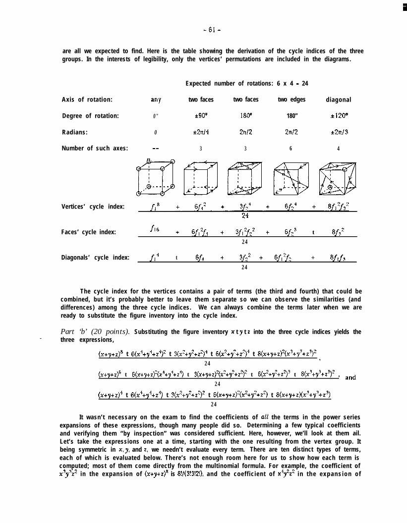
-61-

are all we expected to find. Here is the table showing the derivation of the cycle indices of the threegroups. In the interests of legibility, only the vertices’ permutations are included in the diagrams.

Expected number of rotations: 6 x 4 = 24

Axis of rotation:

Degree of rotation:

Radians:

Number of such axes:

Vertices’ cycle index:

Faces’ cycle index:

Diagonals’ cycle index:

any

0"

0

n

two faces two faces two edges diagonal

k90” 180' 180” i120”

*2n/4 2n12 2n12 *2n/3

3 3 6 4

fi 6 t 6f12f4 f 3fl L.*fn* + 6fz9 t 8f3*24

f14 t q-4 t 3fz2 t 6fr2f? +24

The cycle index for the vertices contains a pair of terms (the third and fourth) that could becombined, but it’s probably better to leave them separate so we can observe the similarities (anddifferences) among the three cycle indices. We can always combine the terms later when we areready to substitute the figure inventory into the cycle index.

Part ‘b’ (20 points). Substituting the figure inventory x t J t z into the three cycle indices yields thee three expressions,

(x+,3tz)8 t 6(x”ty4+z”)” t 3(x’tly”tz2)” t 6(x2t+2)4 t 8(x+ytz)2(x’t$tz3)=24

9

(xtytz)6 t 6(xty+z)*(x4ty4tz4) t 3(Xt~tZ)2(X2t~2tZ2)2 t 6(x"ty2tz2)3 t 8(X3t$kZ3)" , and24

(xtytz)” t 6(x4ty'tz4) t 3(x2t$tz2)2 t 6(xtytz)+c2ty%r2) t 8(xtytz)(x’+y’+z’)24

It wasn’t necessary on the exam to find the coefficients of at1 the terms in the power seriesexpansions of these expressions, though many people did so. Determining a few typical coefficientsand verifying them “by inspection” was considered sufficient. Here, however, we’ll look at them ail.Let’s take the expressions one at a time, starting with the one resulting from the vertex group. Itbeing symmetric in X, y, and z, we needn’t evaluate every term. There are ten distinct types of terms,each of which is evaluated below. There’s not enough room here for us to show how each term iscomputed; most of them come directly from the multinomial formula. For example, the coefficient ofx’J&* in the expansion of (rtytz)8 is 8!/(3!3!2!), and the coefficient of x4r2zT in the expansion of

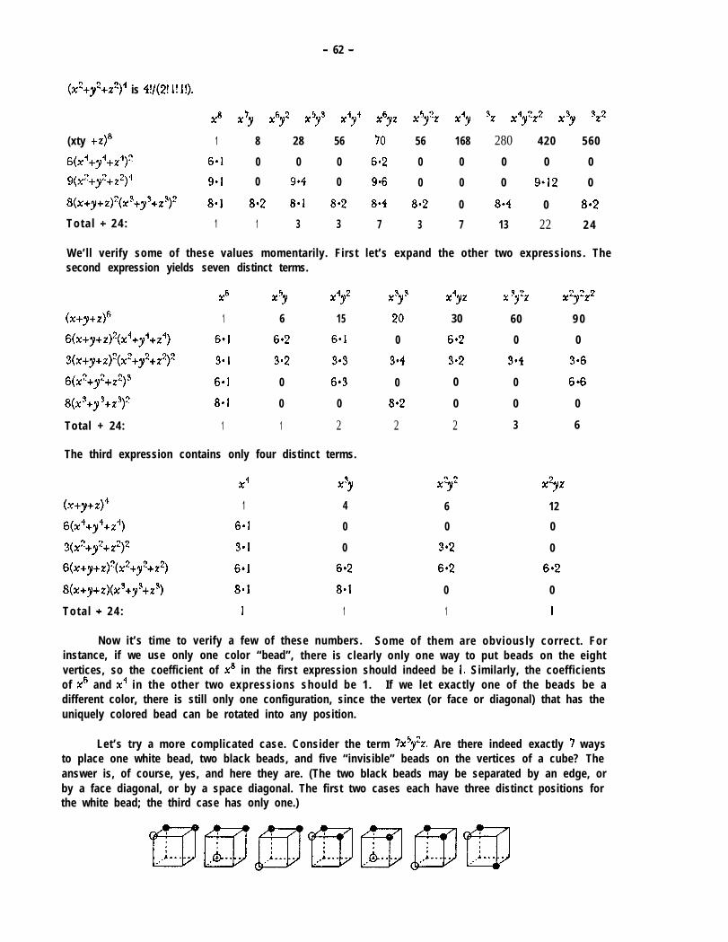
- 62 -

(x2+y2tz2)4 is 4!/(2! l! l!).

$3 x’y #by* x5y3 x4y4 xbyz x5y:r x4y % x4y?z2 x3y 3%*

(xty +zj8 1 8 28 56 70 56 168 280 420 560

G(x’+y’+z”) 6*1 0 0 0 6.2 0 0 0 0 0

9(x2+y’+z2)” 9*1 0 9*4 0 9*6 0 0 0 9*12 0

8(x+y+z)“(xJ+yJ+z’)’ 8*1 8*2 8.1 8*2 8*4 8*2 0 8*4 0 8*2

Tota l t 24 : 1 1 3 3 7 3 7 13 22 2 4

We’ll verify some of these values momentarily. First let’s expand the other two expressions. Thesecond expression yields seven distinct terms.

x6 x5y x4y*

(xty-@ 1 6 15

~(x+~+z)+c~+~~+z’) 6*1 6*2 6.1

3(Xtytz)~(X~ty*tz~)2 3*1 3.2 3*3

6(x’ty%zz)J 6*1 0 6*3

8(&y 3+z3)2 8*1 0 0

Total + 24: 1 1 2

The third expression contains only four distinct terms.

x4 X3J

(xtyt%)4 1 4

6(x4ty4tz4) 6*1 0

3(X%y*trq2 3.1 0

6(se+y+z)“(x2ty2tz2) 6*1 6*2

8(xtytz)(x%y%z’) 8.1 8*1

Tota l + 24 : 1 1

Now it’s time to verify a few of these numbers.

X3Y3 X4YZ X $22 x2Y2z220 30 60 9 0

0 6.2 0 0

3*4 3*2 3*4 3*6

0 0 0 666

8+2 0 0 0

2 2 3 6

X2Y2 x*yr

6 12

0 0

362 0

662 6*2

0 0

1 I

Some of them are obviously correct. Forinstance, if we use only one color “bead”, there is clearly only one way to put beads on the eightvertices, so the coefficient of x8 in the first expression should indeed be 1. Similarly, the coefficientsof x6 and x4 in the other two expressions should be 1. If we let exactly one of the beads be adifferent color, there is still only one configuration, since the vertex (or face or diagonal) that has theuniquely colored bead can be rotated into any position.

Let’s try a more complicated case. Consider the term 7x5y’z. Are there indeed exactly 7 waysto place one white bead, two black beads, and five “invisible” beads on the vertices of a cube? Theanswer is, of course, yes, and here they are. (The two black beads may be separated by an edge, orby a face diagonal, or by a space diagonal. The first two cases each have three distinct positions forthe white bead; the third case has only one.)

- 63 -

What about, in the second expression, the term 2x’yz? If we paint one face white and oneface black (and leave the other four unpainted), there are indeed two distinct configurations. Eitherthe two faces touch along one edge, or they do not touch.

What can we say about the third expression? Each of the coefficients is I; does this makesense? Notice that there are 24 ways we can rotate the cube, and that each rotation permutes thediagonals in a different way. Since there are 4. diagonals, there are only 4! = 24 different ways inwhich they can be permuted. Therefore any permutation of the diagonals can be accomplished bysome rotation in the group, and so any given combination of colors can be applied in only one way.Any other configuration using the same colors can be permuted into the first by one of the 24rotations.

That’s enough “inspection“. Let’s move on to the “open-ended” section.

Part ‘c’ (extra credit, points awarded as rclarranted). One of the very first things we should notice(though, disappointingly, few people did) is that the cycle index for the diagonals is the same as thatfor the symmetric group S4, and that therefore the diagonals’ permutation group must in fact be thesymmetric group. (In the second paragraph above we described the implications of this.) We coulddouble-check this using the formula for finding the cycle index of a symmetric group, but thiswould essentially duplicate page 47 of the notes, so we won’t bother.

Some observations that we can make, but from which it is difficult to deduce any generalprinciples, include the fact that the vertex group included two terms, generated by rotations aboutdifferent types of axes, that had the same cycle form, whereas this did not occur in the other twogroups. Also, each term in the vertex group yields the same coefficient for x5y’ as for x6yz As wesaid, it is not clear what the implications are of these similarities within the vertex group, but theyare certainly worth noting.

We have already pointed out that the number of rotations remains the same regardless of theelements being permuted. We can extend this observation by noting that the number of rotationsabout any given type of axis, or about any single specific axis, is invariant among the three groups.This may appear to be a case of stating the obvious, but it is an important property nevertheless.

One person noted that the fact that the midpoints of the faces of a cube form the vertices ofan octahedron was merely a particular instance of a general useful phenomenon. When two sets

- correspond to one another in this fashion, they will necessarily have the same cycle index under anygiven form of permutat ion . Thus, for instance, if we were to work out the cycle index for thepermutations of the faces of a cube under both rotation and reflection, we would simultaneouslyproduce the cycle index for the vertices of an octahedron under rotation and reflection.

One very significant observation is the correlation between the degree of rotation (expressedin radians) and the corresponding cycle index term. In every instance (at least, every instance in thisparticular problem), a rotation of 2n/k radians yields a permutation whose largest cycle is of order k .In fact, the permutation consists of one or more cycles of order k and perhaps some cycles of order 1,and no others. It is clear why this should be the case. A cycle of order k indicates an operationthat, if performed k times, restores the original state. The operation of rotating an object throughan angle of 2rt/k radians, if performed k times, does indeed restore the object to its original position.Furthermore, repeating the operation fewer than k times will not restore the original position, sothere should be no cycles of order k-l or smaller, except that a cycle can be of order 1, indicating anelement that is not affected at all by this particular rotation.

Having explained why a rotation through 2n/k radians should always yield at least one cycleof order k and no cycles of orders other than 1 and k, we should point out that this is not strictly

- 64 -

true. For one thing, it’s true only of physical rotations of physical objects whose shapes are notsubject to change, That is, if we rotate one part of the object 180°, there mustn’t be some other partthat changes position by only 120”. For another, there are times when a rotation of less than 360’may restore the original position. For instance, if we were to consider the diaEonais of a rotatinghexagon (considering only the three diagonals that join opposing pairs of vertices), we would findthat a 180” rotation causes ail three diagonals to land back in their original positions. This sort ofthing is probably a pathological case, however. In most cases the observation in the precedingparagraph is a valid and useful one.

theOne person pointed

figure inventory beout a useful special case of the general figure inventory. Specifically, let

fW = fi a,x’ = 3 x .Y=O

Since there is only one variable, it means we are dealing with a single “property“, such as “anycolor”. The coefficient, which could be any positive integer constant, is the number of variations onthe property, such as the number of different colors. Substituting this figure inventory into the cycleindex, we find that ail the terms involve xd, where n is the degree of the group. The coefficient of3~~ is the number of distinct configurations in which each element being permuted has been assignedone of the variations on the property. E.g., substituting this figure inventory into the cycle index forthe faces of the cube wouib result in the single term 57x”, indicating that there are 57 distinct waysof painting the faces of a cube, where each face can be painted any of 3 available colors.

One brave soul attempted to present a rough idea of zuhy substituting the figure inventoryinto the cycle index works the way it does. He did a reasonable job, considering the difficulty of theundertaking. Since he was moved to try explaining the theory behind all this, can we do less?Probably. But let’s see what we can do. We won’t try to prove anything here, but we’ll endeavor topresent some insights on what’s happening when the figure inventory is substituted into the cycleindex, and why it might be reasonable to expect it to yield the results it does. If this explanation istoo confusing, then skip it, but we feel it’s worth the try.

Consider the cycle index for rotations of the vertices of a regular hexagon. As we saw insection 6, this cycle index is

f,” t 2f6 t 2fy2 t f0“ t 3f,*fO’t 3fn’- 12

.

We’ll use the figure inventory x t y, representing two types of object. We’ll denote the two types inthe diagrams that follow by circling vertices of one type and leaving the others empty. Let’s supposewe want to find the number of configurations in which exactly two vertices are of type x (circled).We know there are three such configurations.

We don’t have any systematic formula that counts just these three configurations, so insteadwe’ll count something similar, We‘ll count each configuration, rotated in every possible way. Forexample, the center configuration on the preceding page can be rotated according to each of the 12permutations in the group, yielding the 12 configurations shown below. The top left configurationcomes from the identity permutation, the other five in the top row come from rotations around the

- 65 -

center, the leftmost three in the second row result from rotations about axes drawn throughopposing vertices, and the remaining three result from axes drawn through two opposing edges.

ok”dooo

two

As you can see, not all of these configurations “look” different. That is, different rotations can yieldthe same configuration. (The actual rotations are not identical, however. it is only this particularconfiguration that is indistinguishable under these rotations.) We wish to count ail 12 of theseconfigurations, even though some of them look identical to others. If we can count ail 12 of themand likewise count all 12 rotations of each of the other configurations for two circles, we can thendivide by the total number of rotations and we will have the answer we wanted. So let’s see how wecan go about counting these 12 configurations.

W e sta.rt by separating the I2 configurations into two sets. The first set contains as manyconfigurations as possible such that no two of them “look” alike, and the second set contains the rest.In this particular example, the first set could contain the top row of six configurations, and thesecond set the second row. In general, however, the two sets need not be the same site. What doesit mean for a configuration to be in the second set? It means there is a configuration in the first setthat looks the same, i.e., has the same vertices circled. This means there are two distinct rotationsthat permute the “original” orientation (upper left corner of the twelve above) into this form. (Wecan see that the two rotations are indeed distinct, and hence the resulting look-alike configurationsare in fact different, by numbering ail six vertices instead of merely circling two of them.) Since thetwo rotations are distinct, there must be a rotation, not the identity permutation, that maps theconfiguration in the first set into that in the second set. For instance, the bottom left configurationabove, which resulted from a rotation about an axis drawn through the top and bottom vertices,“looks” the same as one in the top row, which resulted from a 120” rotation counterclockwise aboutthe center. This latter configuration can be permuted into the former by rotating it about an axisdrawn through the upper left and lower right vertices, as shown below.

Each configuration in the second set, then, can be derived by taking a configuration in thefirst set and applying a rotation that doesn‘t change the “appearance” of the configuration. Whenwe perform a rotation that interchanges the two circles, the appearance is unchanged even thoughwe have generated a different configuration. Furthermore, if we have any rotation that doesn‘tchange the appearance of some configuration, and the configuration is in the first set, we can applythe rotation to that configuration and come up with another configuration, which must be in thesecond set. Therefore we have established a one-to-one correspondence between the configurationsin the second set and rotations that do not change the appearance of some configuration.

Observe that, if we consider all distinct configurations (in this case there are 3 of them) andlook at all their rotations, the resulting set of configurations must include all possible combinations

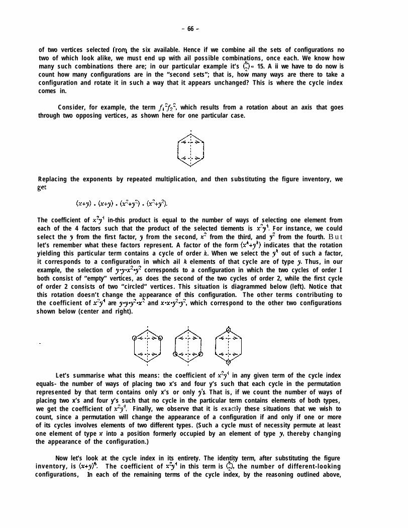
- 66 -

of two vertices selected fronl the six available. Hence if we combine ail the sets of configurations notwo of which look alike, we must end up with ail possible combinations, once each. We know howmany such combinations there are; in our particular example it’s (9) = 15. A ii we have to do now iscount how many configurations are in the “second sets”; that is, how many ways are there to take aconfiguration and rotate it in such a way that it appears unchanged? This is where the cycle indexcomes in.

Consider, for example, the term fl:f22, which results from a rotation about an axis that goesthrough two opposing vertices, as shown here for one particular case.

Replacing the exponents by repeated multiplication, and then substituting the figure inventory, we

get

(sty) l (⌧ty) l (⌧2ty2) l (⌧2ty2).

The coefficient of x’$ in-this product is equal to the number of ways of selecting one element fromeach of the 4 factors such that the product of the selected tiements is x’j! For instance, we couldselect the y from the first factor, y from the second, x’ from the third, and y* from the fourth. B u tlet’s remember what these factors represent. A factor of the form (x’tf’) indicates that the rotationyielding this particular term contains a cycle of order k. When we select the yk out of such a factor,it corresponds to a configuration in which ail k elements of that cycle are of type y. Thus, in ourexample, the selection of y7&yz corresponds to a configuration in which the two cycles of order Iboth consist of “empty” vertices, as does the second of the two cycles of order 2, while the first cycleof order 2 consists of two “circled” vertices. This situation is diagrammed below (left). Notice thatthis rotation doesn’t change the athe coefficient of x?y’ are y3’sy’*x !

pearance of this configuration. The other terms contributing toand a~$*~~, which correspond to the other two configurations

shown below (center and right).

-@@@

,

Let’s summarise what this means: the coefficient of ~‘9’ in any given term of the cycle indexequals- the number of ways of placing two x’s and four y’s such that each cycle in the permutationrepresented by that term contains only x’s or only y’s, That is, if we count the number of ways ofplacing two x’s and four y’s such that no cycle in the particular term contains elements of both types,we get the coefficient of &y’. Finally, we observe that it is exactiy these situations that we wish tocount, since a permutation will change the appearance of a configuration if and only if one or moreof its cycles involves elements of two different types. (Such a cycle must of necessity permute at leastone element of type x into a position formerly occupied by an element of type y, thereby changingthe appearance of the configuration.)

Now let’s look at the cycle index in its entirety. The identity term, after substituting the figureinventory , is (x+y)“.configurations,

The coefficient of x’y” in this term is ($, the number of d i f ferent - lookingIn each of the remaining terms of the cycle index, by the reasoning outlined above,

- 67 -

the coefficient of x2$ is equal to the number of ways in which the rotation corresponding to thatparticular term can transform one of these (9) configurations into another configuration that looksthe same but is really a different permutation of the six vertices. When we sum over all the termsin the cycle Index, the coefficient of x2$ thus comes out to be the number of distinct configurations(in our example, 3), multiplied by the number of rotations that can be applied to each of theseconfigurations (in our example, 12). We divide by the number of rotations and there’s our answer.

We hope the preceding discussion provides some faint illumination as to the inner workingsof Polya’s Theory o f Count ing . This is really the sort of thing that should be discussed in muchgreater detail, with much greater formality, and in the interactive setting of a classroom. Lackingthe time for this, however, we hope that this has given you at least some insight into the theoryunderlying the method.

Problem 2 (20 points total).

Part ‘a’ (20 points). The identity to be proved in this problem is actually true only when m and nare non-nega.tive integers. Fortunately, everybody seemed to reaiise this, so our failure to mention iton the midterm handout didn’t lead to any difficulties. Three different forms of “proof” showed up

among the papers handed in. One of these methods is not quite valid, and a few points werededucted for using-it. We’ll present it here in order to be able to point out what’s wrong with it.

It typically ran something like this. We know, by the recursive definition of the binomialcoefficients, that

(“:‘, = (,_n,) + t:,for any integers n a n d r such that 0 < r < ntl. This equation continues to hold even if r > n+l( a s s u m i n g nt l>O), if we assume (i) = 0 whenever J and t are integers and 0 I 5 < t. T h i s i s areasonable assumption to make, since after all there are zero ways to choose a subset of C elementsfrom a set with fewer than t elements. By repeated application of this formula, we deduce that

($1 - (;) + &R+,)- t:,, + c’y, + (1;:)- t;, + T’y, + Ti2) + (i;:,..- ($+ (y) + (n;2) + ’ ’ ’ + (Z, + (mo+,).

- A s s u m i n g m L 0, (,“,,) must be zero, so we find that

(:‘,I, = (i) t r;‘) t (n;2, t ’ ’ * t cp, - i: (i,,k=Owhich is the desired identity. The problem with this “proof” is that it’s not really a formal proof,since it involves an indefinite number of steps. The above argument would suffice in an informaldiscussion, or perhaps as an answer to a request to “show” instead of “prove”, but in a proof youshould be a bit more cautious. One reason this was emphasised so much in grading the midterm isthat, if you’re not careful, such an approach can result in “proving” things that are in fact false!The problem can arise in two ways. You may fail to observe that one of the steps glossed over inthe “ . . . ” is a special case for which the general equation doesn’t apply, or you might attempt to usethe “ . . . ” to represent an infinite sequence of steps. Mathematical induction, which is the formal

- 68 -

representation for this sort of proof, proves things only for any finite number of repetitions of theinductive step. It is not difficult to find statements that are true for any finite n, and can be provedby induction, but are false if n is infinite.

Anyway, that’s enough about that. Here’s the formal proof using induction. We first consider‘the case n - 0. In this case,

t:yJ I= (,) - Q + !,“,,, = Q = 2 tklk - 0 m

(since (,9,) - 0). So the formula is true for ail m when n - 0. Now we assume that it’s true for allnon-negative integers n s J for some value s. We need to show that the formula is then true forn - 54.

t;‘+“) - t;;, = cp’, + (Z’,, [by the recursion formula]

- c:‘, + i (;Ik=O

s+ I- c (i,

k=O

[by the induction hypothesis1

By induction, then, the formula is true for any finite integer n L 0.

One never knows what interesting things will turn up on an examination paper. Two peoplefound a completely different way of approaching this problem. Their method is quite valid and ’reasonable, and it is interesting enough to warrant our reproducing it here. It uses generatingfunctions instead of induction. (These are, after ail, the two most common ways of dealing with anarbitrarily large sequence of values.) We introduce the following generating function involving m asthe exponent:

g<x, - 2 (i tk)) Xrn*m=O k=O m

We first interchange the order of the two summations.

g(x) = 5 i? (‘) Xrnk-0 mr0 mThe terms for m > k are zero, so we can apply the binomial theorem and find

g(x) = E ( wk,k=Owhich is simply a geometric series. We know what the sum of a geometric series is-we encounteredit in section 3 of the notes (pages 8-9). So

&) - 1 - ( l+X)n+'

1 - (Itx)

p (I+$+' - 1

x

- x-'[ (5; (",", xk) - I].tc

In this new summation, the term for k - 0 is (ni’)xo - 1, so we can cancel this against the “-1” thatfollows the summation.

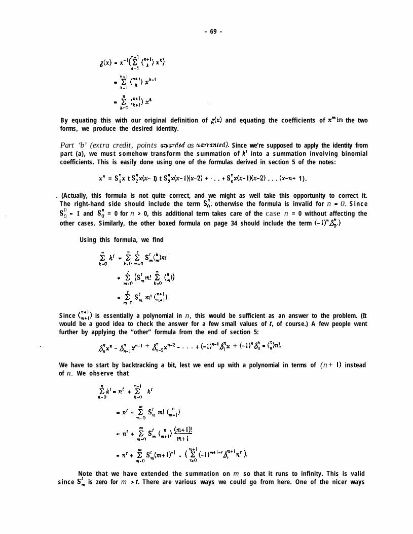
- 69 -

- 2’ cql) %k-l

k-l

By equating this with our original definition of g(x) and equating the coefficients of xrn in the twoforms, we produce the desired identity.

Part ‘b’ (extra credit, points awarded as ruarranted). Since we’re supposed to apply the identity frompart (a), we must somehow transform the summation of k’ into a summation involving binomialcoefficients. This is easily done using one of the formulas derived in section 5 of the notes:

x” = Syx t SL@x- I) t Qc(x- 1)(x-2) + e . . t SIX-1)(x-2) . . . (x-n+ 1 ) .

. (Actually, this formula is not quite correct, and we might as well take this opportunity to correct it.The right-hand side should include the term S:; otherwise the formula is invalid for n = 0. S i n c eSE - I and S: = 0 for n > 0, this additional term takes care of the case n = 0 without affecting theother cases. Similarly, the other boxed formula on page 34 should include the term (-1)“,$.)

Using this formula, we find

i kf = 5 i Sk(,)m!k=O k-0 me0

u i (Sfp! kio (i,>m=O cz

Since (i’,)) is essentially a polynomial in n, this would be sufficient as an answer to the problem. (Itwould be a good idea to check the answer for a few small values of 1, of course.) A few people wentfurther by applying the “other” formula from the end of section 5:

- gp _ ~~-lx~-l + f2p-2 - . . . + (-l)n-i&t + (-l)“& - ()z!.

We have to start by backtracking a bit, lest we end up with a polynomial in terms of (n+ 1) insteadof n. We observe that

3 k’ = n’ t r!i k’k=O= 72’ + m!Zo St, m! (,1,)

= n’ t mto Sa(mt I)” l ( y( (-l)m+‘-r~~+‘nr 1.e

Note that we have extended the summation on m so that it runs to infinity. This is validsince St, is zero for m > t. There are various ways we could go from here. One of the nicer ways

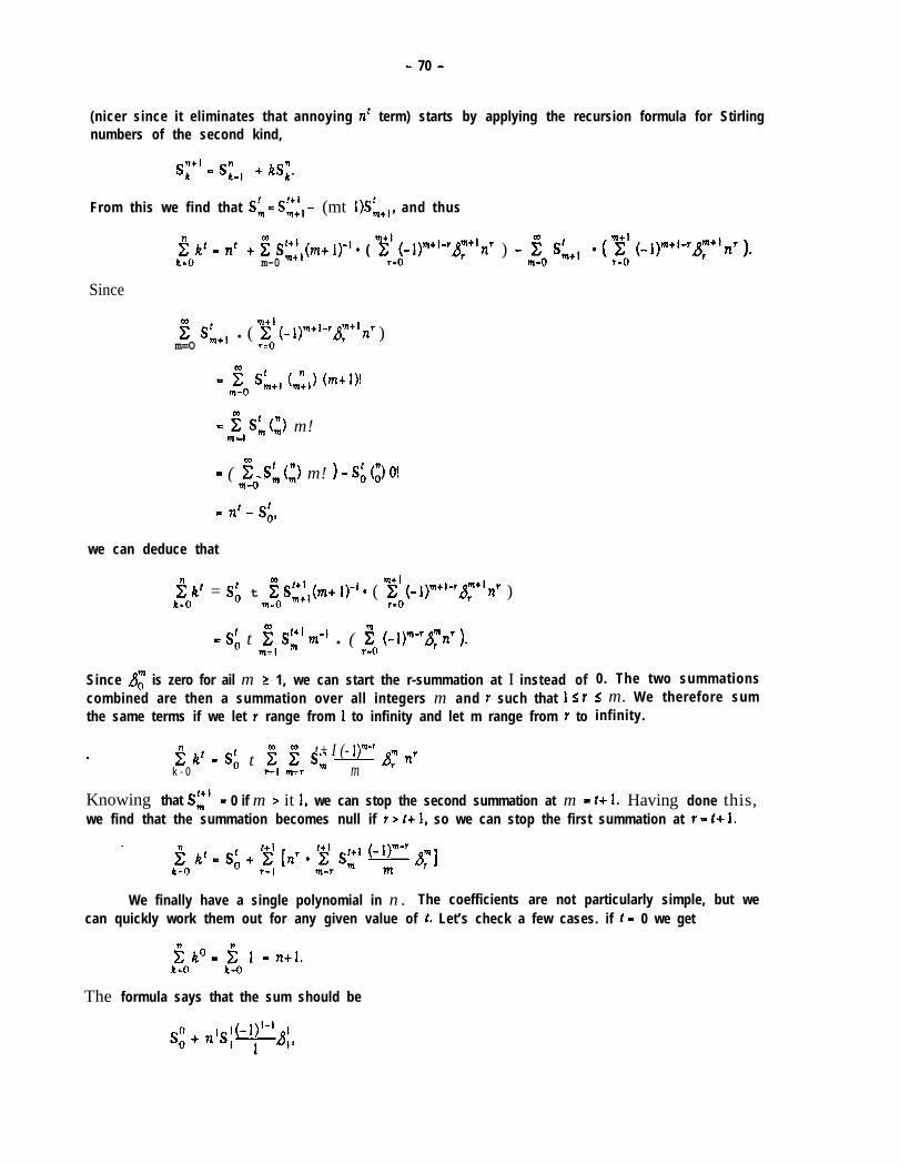
- 70 -

(nicer since it eliminates that annoying n’ term) starts by applying the recursion formula for Stirlingnumbers of the second kind,

s;+’ = s;-, t ks;.

From this we find that SL = Sag, - (mt l)S’,+,, and thus

Since

f It’ - n’ t : SEi,(mt I)” * ( 5’ (-l)m’iwr$“n’ ) - i. SL+,k-0 m-0 r-0

5 %l+lm=Ol ( y$i (-l)m+‘-rJ~+‘nr )

= IE, Sk+, <,“,J h+O

= jt, Si (fJ m!L

= ( j$S~ (z) m! ) - Sb (z) O!e

= n’ - s;,

we can deduce that

3 kr = Si t E S~~,(mt I)” e ( y’ (-l)m’i*r#+‘nr )k=O m-0 r=O= Si t mtl Si’ m-I l ( jfio (-l)a-r&32’ ).e

Since fi: is zero for ail m 2 1, we can start the r-summation at I instead ofcombined are then a summation over all integers m and Y such that I s Y

the same terms if we let Y range from I to infinity and let m range from Y to

t+ I (- l)m-ri k’ = S; t rt, m$r S, -k - 0

s,” n’- - m

0. The two summationsI m. We therefore suminfinity.

Knowing that Sz’ = 0 if m > it I, we can stop the second summation at m = tt I. Having done this,we find that the summation becomes null if Y > tt I, so we can stop the first summation at Y = t+l.

We finally have a single polynomial in n . The coefficients are not particularly simple, but wecan quickly work them out for any given value of t. Let’s check a few cases. if t = 0 we get

5 k”-k$c’l =ntl.k=O -

The formula says that the sum should be

- 71 -

which does indeed equal nt 1. For t - I we know that

$. k’ = 5 (f, - (‘f;‘)k=O 4

by using the formula from part (a). We expect this to equal

= 0 t tn t tn2 I

which again checks. The formulas for i = 2 and t - 3 work out to be

5k-0 k2uot!!t~t~en(nt~~2nt~) 6 2 3

a n d k$$o k” = 0 t 092 t -t ”n2r 4

Tt $= (f k)2,k=Owhich also turn out to be correct.

One person computed some of the individual coefficients. The coefficient of n’+’ (which isthe highest power of n for which the coefficient is non-zero} is always l/(tti). More surprisingly,for t > 0, the coefficient of n’ is always !, independent of Z. This person went on to comment, “Itturns out that following coefficients can be expressed in terms of Bernoulli numbers, but this isprobably beyond the scope of the midterm.” She was quite right-on both counts.

Problem 3 (30 points total).

Let us denote the n digits in any particular n-digit number by the variables d,, d2, . . . , dn. H o wmany such numbers do not start with a zero and have no adjacent pairs of digits alike? Let us findthe answer first without using PIE.

The first digit (d,) can be any digit other than a zero. Thus it has 9 possible values. Thesecond digit, d,, can be any digit different from dl. Thus, for each possible value of d,, d2 also has9 possible values. Similarly, for any digit d, there are 9 possible values, regardless of the values of

- the other digits. (The 9 possible values depend on the values of the other digits, but there arealways 9 of them.) By the product rule from way back in section 2, then, the total number ofcombinations must be

ii 9,I=’

which is simply 9”. That was easy; now for the hard part! (Even though this problem is easier tosolve without PIE than with it, we felt it was worth including on the midterm. It’s not particularlycomplicated even using PIE, and it lets you check your result using the non-PIE approach.)

Most people did fairly well applying PIE to this problem. Those who didn’t seemed confusedas to exactly how PIE works. Several people simply defined Ndl, Ng, etc., without specifying exactlywhat a , b, e tc . , were . One particularly popular mistake was defining Na to be the number ofn-digit numbers with at least one pair of adjacent digits alike, No the number of numbers withsome three adjacent digits alike, and so forth. This approach quickly runs into trouble when itcomes time to define Na4. People who somehow managed to hedge past this found that numberssuch as “3344”, containing two different pairs of matching digits, were counted twice by No but not

- 72 -

at a l l by N4, N , , etc., resulting in an answer that was too small for n L 4.

Here are some rules of thumb to keep in mind any time you intend to use PIE:

111 Start b y establishing exactly what you intend to have as the properties a, 0, etc.

I23 The union of these properties (that is, the union of the sets of elements having each property)must consist of precisely those elements that you’ do not wish to count.

[33 Try to choose properties that are “interchangeable”. That is, try to arrange things so thatNdl = Ng = l l . = Nh, and NQb = N,, = N8? = . e e , and so forth. This sort of symmetry willmake the PIE formula much simpler to evaluate.

[4l Choose 01, 0, and the other properties such that the individual terms (N,, No, . . . , N,o, etc.)are easy to evaluate.

For this particular problem, we will let aI be the property that d, is the same as dl, a2 theproperty that ds is the same as d:, . . . , and in general at the property that d,,, is the same as d,.There are a total of n-l such properties. This clearly follows rules El3 and 121 above; we’ll soon seethat 131 and [4] are also met.

Consider any combinat ion of k proper t ies: cq,, afs,. . . , af4. How many n-dig i t numbershave this particular set of properties? That is, what is N(al,,u12,...,al,)? (Pardon our not usingsubscripts on the N, but subscripts on subscripts on subscripts are absolutely illegible!) The firstdigit, d,, can still be any digit other than zero. Each of the remaining n-l digits can be any of theten decimal digits, except that exactly k of them are constrained to be the same as their immediate1preceding digits. Thus there are 9*10n”‘k Ysuch n-digit numbers, and N(ar,,al,,...,ai,) - 9*10n-‘- .Furthermore, since there are n-l properties, there are (“ii) such terms. This formula is valid evenwhen k - 0; that is, there are a total of 9’10”” n-digit numbers.

Applying the PIE formula, we find

No - 9’10”’ . (n-l)egel()n’2 + (n;‘)~g~~On-9 - . . . f (~-~)+elO”m

I g e 1%; (";I) (-l)k l(y"'k

e

a

= 9 l (lO-l)n-’

by the binomial theorem. So No = 9” as expected.

rl9 Ramsey Theory

Februury 23. This was Tarjan’s first lecture, and he started by announcing what he intended tocover during his seven lectures. Specifically, he said he would be discussing miscellaneous problemsin existential and constructive combinatorics, with the emphasis being on the constructive side. Thissection, on the other hand, deals almost entirely with existential combinatorics, although some of theproofs are constructive.

We encountered Ramsey Theory briefly in section 7, where we looked at one of its simplestcases. If there are six people at a party, either there are three people who know each other or there

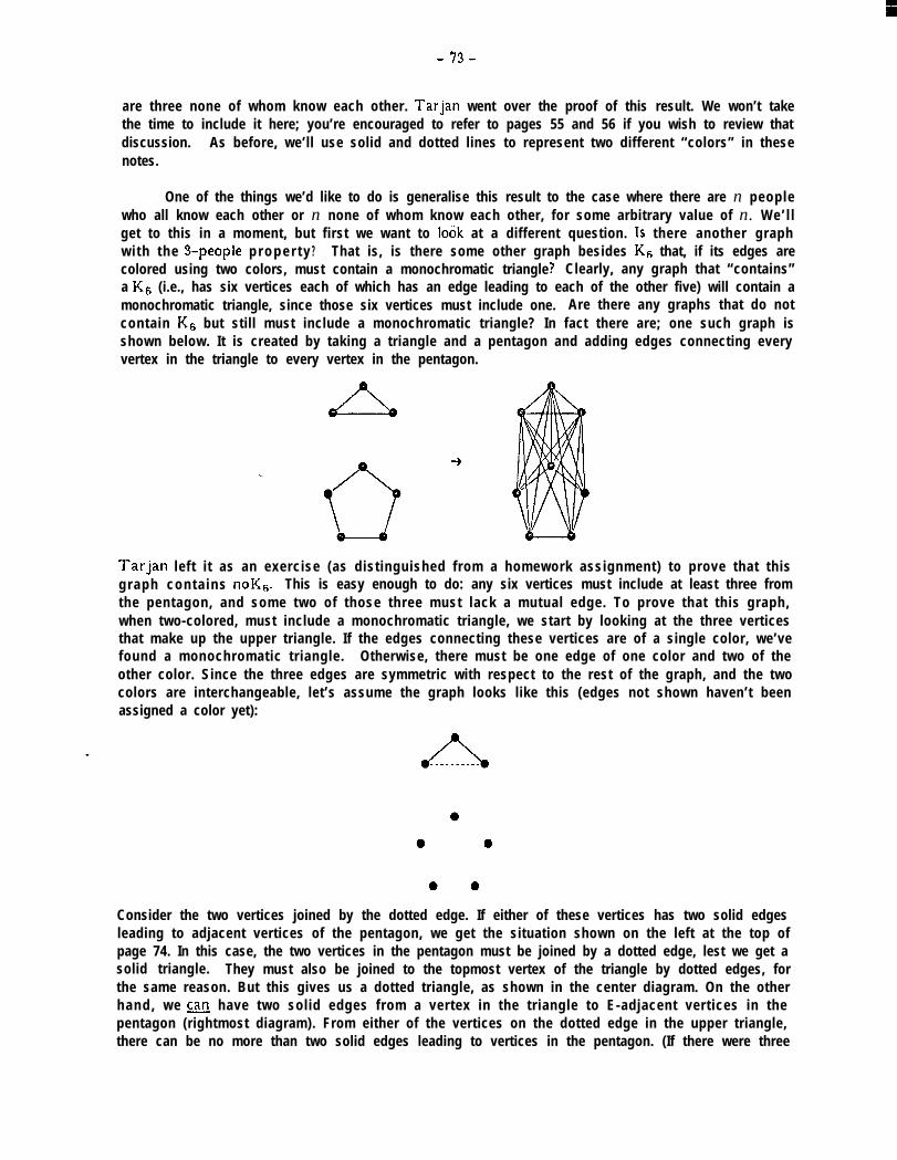
- 73-

are three none of whom know each other. Tarjan went over the proof of this result. We won’t takethe time to include it here; you’re encouraged to refer to pages 55 and 56 if you wish to review thatdiscussion. As before, we’ll use solid and dotted lines to represent two different “colors” in thesenotes.

One of the things we’d like to do is generalise this result to the case where there are n peoplewho all know each other or n none of whom know each other, for some arbitrary value of n. We’l lget to this in a moment, but first we want to look at a different question. Is there another graphwith the 3-people p r o p e r t y ? That is, is there some other graph besides K6 that, if its edges arecolored using two colors, must contain a monochromatic triangle ? Clearly, any graph that “contains”a K6 (i.e., has six vertices each of which has an edge leading to each of the other five) will contain amonochromatic triangle, since those six vertices must include one. Are there any graphs that do notcontain K6 but still must include a monochromatic triangle? In fact there are; one such graph isshown below. It is created by taking a triangle and a pentagon and adding edges connecting everyvertex in the triangle to every vertex in the pentagon.

Tarjan left it as an exercise (as distinguished from a homework assignment) to prove that thisgraph conta ins no Kg. This is easy enough to do: any six vertices must include at least three fromthe pentagon, and some two of those three must lack a mutual edge. To prove that this graph,when two-colored, must include a monochromatic triangle, we start by looking at the three verticesthat make up the upper triangle. If the edges connecting these vertices are of a single color, we’vefound a monochromatic triangle. Otherwise, there must be one edge of one color and two of theother color. Since the three edges are symmetric with respect to the rest of the graph, and the twocolors are interchangeable, let’s assume the graph looks like this (edges not shown haven’t beenassigned a color yet):

Consider the two vertices joined by the dotted edge. If either of these vertices has two solid edgesleading to adjacent vertices of the pentagon, we get the situation shown on the left at the top ofpage 74. In this case, the two vertices in the pentagon must be joined by a dotted edge, lest we get asolid triangle. They must also be joined to the topmost vertex of the triangle by dotted edges, forthe same reason. But this gives us a dotted triangle, as shown in the center diagram. On the otherhand, we can have two solid edges from a vertex in the triangle to E-adjacent vertices in thepentagon (rightmost diagram). From either of the vertices on the dotted edge in the upper triangle,there can be no more than two solid edges leading to vertices in the pentagon. (If there were three

- 74 -

solid edges they would necessarily include two leading to adjacent vertices.) Thus each of these twovertices in the triangle has at least three dotted edges leading to the pentagon. This makes a total of

0 0 0 0 0 0

six dotted edges, so at least two of them must go to the same vertex in the pentagon. These twoedges, together with the dotted edge in the upper triangle, form a.monochromatic triangle.

As homework, Tarjan asked for a proof that if the edges of K6 are two-colored there must beat least two monochromatic triangles. The resulting homework papers included almost as manydifferent proofs as there were papers. Here is a typical proof. We start by taking advantage of thefact that we already know there must be at least one such triangle. Let’s assume it’s solid, and drawthe graph with those three vertices at the top, as shown on the left below. Each vertex of thetriangle must have at J&t one additional solid edge. (Jf any vertex of the triangle has ail threeremaining edges dotted, we get the situation shown in the center diagram below, in which case eitherthe three bottom vertices are ail connected by solid edges, creating a second triangle, or some two ofthem are connected by a dotted edge, creating a dotted triangle.) If any vertex in the first trianglehas more than one additional solid edge, we get the situation shown on the right below, in which weeither have a dotted triangle as shown, or one of the edges shown as dotted must instead be solid,giving a solid triangle. Thus, for each of the points of the first triangle, the three remaining edges

0 0

0

must include exactly one solid edge and two dotted edges. In addition, each of the three additionalsolid edges (one from each vertex of the triangle) must go to a different vertex, lest we get anothersolid triangle (below left). Since the three lower vertices are indistinguishable at this point, we getthe situation shown in the center diagram below. If we are to avoid having another solid triangle,certain edges must be dotted, as shown on the right below, But then, if we are to avoid getting adotted triangle, each edge connecting two of the three lower vertices must be solid. This gives us asecond solid monochromatic triangle. This construction also shows that it is possible to two-color aKG so as to have exactly two monochromatic triangles. It is not known, for general n, what theminimum number of monochromatic triangles is in a two-colored K,.

Getting back to the case of proving the existence of a single monochromatic triangle in K6,how can we generaiise this result and its proof? How large must a graph be so that when its edges

- 75 -

are two-colored there is a complete monochromatic subgraph of k vertices? (A triangle, of course, isa complete graph of 3 vertices.) This time it was Tarjan’s turn to come up with a problem-solvingaphorism: “Sometimes to get a result you have to ask a more general question.” in order to prove thata sufficiently large graph always exists, we must generaiise the problem still more.

We def ine R(m,n,2) to be the minimum integer such that, if IV 2 Y?(m,n,2) and each edge ofJcN is “colored” solid or dotted, then there is either a solid K, or a dotted K,. (The “2” denotesthat we’re coloring edges, which correspond to p’airs of vertices. This will be important later.) Jt isassumed that m and n are positive integers. We saw in section 7 that it is possible to two-color a KI,graph without getting any monochromatic triangles, and that a two-colored I& always has such atriangle, so we know that %(3,3,2) = 6. What other values of Y? can we readily ascertain? Consider‘R(m,2,2). If we have a K,, 1 graph, we can color ail its edges solid, and we will have neither a solidK, nor a dotted KF. If we two-color the edges of K,, however, then either we have a dotted edge(which would be a dotted K:, since Kz is a single edge) or else ail the edges are solid, giving us asol id K,n. Therefore R(m,2,2) = m. Simi lar ly , Yl(2,n,2) - n. ( In general, Y?(m,n,2) = gZ(n,m,2), sincethe definition is symmetric with respect to rn and n.)

We now come to Ramsey’s Theorem, version 1: For ail m a n d n 2 2, R(m,n,2) exists andsatisfies the relation

R(m,n,2) 5 Yl(m,n- I,21 + Wm- h2)

for ail m and n r: 3.

The proof is by induction on the suln m+n. We know, when m and n are 2 3 and m+n = 6,that we must have m = n - 3 , and that R(3,3,2) = 6 5 3 + 3 - !9(3,2,2) + YI(2,3,2). S o f a r s o g o o d .Now suppose the theorem is true for mtn c t, and consider the case when mtn = t. Suppose thatN L R(m,n-1,2) t Yl(m-i,n,2) and that the edges of KN are colored solid or dotted. Pick any vertex;it is connected to every other vertex, and there are at least Y?(m,n-1,2) t YR(m-l,n,2) - I of them. Oft h e s e R(m,n-1,2) + R(m-l,n,2) - 1 edges, either at least Y!R(m,n-1,2) of them are dotted, or at leastR(m-l,n,2) of them are solid. Why is this? Well, if it weren’t so, then there would be at most!R(m,n-1,2) - I dotted edges, and at most !J&-l,n,2) - I solid edges. But this would give a total ofat most R(m,n-1,2) t R(m-I,@) - 2 edges, and we’ve said there must be at least one more than that.So suppose !R(m-l,n,2) of the edges are solid. Consider the vertices at the “other ends” of theseedges. (Remember that ail these edges are coming from a single vertex.) According to our inductionhypothesis, these R(m-l,n,2) vertices and their interconnecting edges must include either a solid K,,,

- or a dotted J<,. If the latter, we’re done, since the original K,,, contains this same K,. If there’s asol id K m+ t h e n t h e origina. KN contains a solid K, consisting of these m-l vertices together withthe vertex we selected at the start, since that vertex is known to be connected by solid edges to eachof the m-1 vertices. The case when the vertex we start with has R(m,n-1,2) dotted edges is handledsimilarly, and is left as an exercise.

You should be sure you understand the above proof before proceeding; the same approachwill be used to prove the more general versions of Ramsey’s Theorem later on. Notice how thisproof generaiises the method used to determine R(3,3,2). Note also that the proof forces us toconsider Y?(m,n,2) for m # n.

Using this theorem, we can compute upper bounds on the values of the Ramsey numbersY?(m,n,2). Here’s a table showing these bounds for the first few values of m and n.

.

- 76 -

j-+%

These values should look familiar-they are simply‘ the binomial coefficients. This isn’t terriblysurprising, since the upper bound given by the theorem is the same as the recursive definition of thebinomial coefficients. Ramsey’s Theorem (version 1) tells us that R(m,n,2) < (“i_“;‘). On the otherhand, certain Ramsey numbers (not many) are known precisely. The following table, taken from[Hararyl, shows all the values currentty known (not counting cases where m or n = 2, and omittingsome values which are identical to others by symmetry).

Ytbm2)

j-p+

Notice that the bound given by the theorem gets progressively worse. There is no general methodknown for finding these (and hence additional) numbers. Computing a few more entries for theabove table is usually sufficient for a thesis; finding a general method would bring instant fame (at

.ieast within the world of mathematics).

How can we generaiise this idea still further? We’ve pointed out that, in coloring the edges,we’re actually assigning a color to each pair of vertices (where two pairs sharing a common vertexdoes not imply that the two pairs must be assigned the same color; it is the pairings that are beingassigned colors, not the individual vertices). Suppose we instead assign a color to every possiblesubset consisting of Y vertices? We shall call such a set an r-subset.

We define R(m,n,r) to be the minimum integer such that, if each r-subset of a set containingN r: R(m,n,r) elements is colored either solid or dotted, then either there is an m-subset ail of whoser-subsets are solid, or there is an n-subset ail of whose r-subsets are dotted. As an example, let T be

-3, and suppose we have a set of five elements, {a,b,c,d,ej. There are (,“, = 10 3-subsets. If we let thesix subsets (a&c), (a,B,d), (a,c,n), (a,c,e), (a&e}, and (c,&e} be “solid”, and the remaining four 3-subsets“dotted”, then there is a 4-subset, (a,c,d,ej, such that ail 3-subsets of this 4-subset are solid. On theother hand, it is certainly possible to assign “colors” to the 3-subsets in such a way that there is nosuch 4-subset, so R(4,4,3) is not 5. (In fact, no one knows what the value of R(4,4,3) is!)

Let’s look at some special cases for which the values of Y?(m,n,r) are known. For instance,what about R(m,r,r)? We claim R(m,r,r) = m. (It is obvious that jR(m,r,r) cannot be less than m.) Ifwe have a set of m (or more) elements, then either there is at least one dotted r-subset, in which casethose Y elements form an r-subset “ail of whose r-subsets are dotted” (an r-subset has only oner-subset, namely itself), or else ail of the r-subsets are solid, in which case we have m elements ail ofwhose r-subsets are solid. Similarly, by symmetry, $R(r,n,r) = n. Suppose Y = I? In this case we aresimply coloring each of the vertices individually. We claim !J?(m,n,l) = m+n- 1 for ail m and n 1 1.If a set has this many elements, and each is colored either solid or dotted, then we must have eitherm solid or n dotted elements. If we didn’t, then we could have at most m-l solid and n-l dottedelements, which accounts for only mtn-2 of them. This special case of Ramsey’s Theorem (whichwe’re about to state in its general form) is called the pigeonhole principle: if we distribute mtn-1

- 77 -

objects into two categories, either the first category contains m or more objects or else the secondcategory contains n or more objects. There’s another form of the pigeonhole principle; we’ll come toit eventually.

We’re now ready to look at Ramsey’s Theorem, version 2: For ail m and n 2 Y 1 I, ?R(m,n,r)exists and satisfies the relation

Wmr) S WR(m,n- l,r),!l?(m- l,n,r),r- 1) + 1

for ail m and n > Y > 1.

Before proving this theorem, let’s check it for the case Y = 2. According to the theorem,R(m,n,2) s !R(R( m,n-1,2),R(m-],@),I) t 1 - [~(m,n-1,2)t~(m-1,n,2)-1~ t 1 ( a c c o r d i n g t o o u r f o r m u l afor !R(m,n,l) ), so this checks against the first version of the theorem. How can we prove this newtheorem in general?

L e t p = !R(m- l,n,r) and q = R(m,n-l,r), and assume N 2 R(p,q,r-1)t 1. Suppose S is a set of IVelements, and that the r-subsets of S have been colored solid and dotted. Pick any element v in Sand consider the r-subsets that contain v. Each one corresponds to an (r-l&subset of the N-lelements that do not include v. (Let SO represent the subset S-(v), which is the same as S except thatv has been removed.) A coloring of the r-subsets of S that include v corresponds to a coloring ofthe (r-l&subsets of‘& that do not include v. Since N-1 L Y?(p,q,r-I), we know that there is either asubset of p elements of S ,-,, ail of whose (Y-I)-subsets are solid, or there is a subset of q elements ofSo, ail of whose (r-I)-subsets are dotted. The two cases are similar; consider the first. In this casewe have p = J?(m-l,n,r) elements, each of whose (r-I)-subsets is solid. This corresponds to thecoloring of the r-subsets of S in which each (r-l)-subset of the p elements, when taken together withv, forms an r-subset that is solid. Meanwhile, by the definition of R(m-l,n,r), there must be eitheran (m-I)-subset of the p, ail of whose r-subsets are solid, or else an n-subset ail of whose r-subsetsare dotted. In the latter case, we’re done. In the former case, we take the m-l elements together withv, and thereby find an m-subset ail of whose r-subsets are solid.

Finally, let’s generaiise to include the situation where there are more than two colors. Wedefine W(n, ,n2, . . . ,n,,r) to be the minimum integer such that, if each r-subset of a set containingN 2 !R(nl ,n?, . . . ,n,,r) elements is colored with one of t colors, then there is some i such that someq-subset has ail its r-subsets colored using the ith color.

- One more time! This time it’s Ramsey’s Theorem, version 3: For ail nl, n2, . . . , n, L Y 2 1,!R(ni,n2, . . , ,n,,r) exists and satisfies the relation

R(nl ,n2, . . . ,n,,r) I !R(!R(n I ,112, . e . ,n,-1 ,r),n,,d

- f o r t > 2 .

To prove this, we group the colors into two categories. The first category contains the first t-lcolors and the second category the last color. Given a set of N 1 Y?(Y?(nI,n2, . . . ,n,+r),n,,r) elementswhose r-subsets have been colored using t colors, we take every r-subset that has been colored usingany of the first t-l colors and color it “solid” instead. By the definition of the two-color case, weknow that either there is an q-subset ail of whose r-subsets are dotted, or else there is a subset ofRh ,nz, . . . ,ntwl,r) elements ail of whose r-subsets have been colored using only the first t-l colors.The theorem follows by induction.

For instance, we can get the following bound on the value of ?RCW,2):

- 78 -

R(3,3,3,2) s R(R(3,3,2L3,2) = YWt392) - 18.

(The earlier versions of the theorem told us only that !J?(6,3,2) was I: 21, but it has in fact beenfound that it is 18, so we can get a slightly better bound on the value of $?(3,3,3,2).) The ac tua lvalue of R(3,3,3,2) is known to be 17. There’ll be more to say about that on the final exam.

As a special case, we find !R(2,2,2, . . . ,2,1) = ttj (where there are t co lors) . Th is is anothercase of the pigeonhole principle: if we distribute it 1 objects into 1 categories, some category mustcontain two or more objects. Ramsey Theory is in a sense just a generaiisation of the pigeonholeprinciple.

For people interested in further reading concerning Ramsey Theory, Tarjan suggested threereferences: [Hail], pp. 54-57, [Ryserl, pp. 38-46, and [Hararyl, pp. 15- 17.

Before moving on to section 10, let’s look at some applications of Ramsey Theory. (Thismaterial was not covered in the lecture. This section of the notes is based on some lecture notesprepared by Tarjan that he never found time to present.)

A finite semigroup is a finite set on which a binary associative operation is defined. Theoperation is referred to as “multiplication”, although in fact it may not be the ordinary arithmeticmultiplication operation. For instance, given any finite set S, we can take the collection of ail subsetsof S, together with the operation of set union, and that will form a finite semigroup. (We could alsouse set intersection as the semigroup operation.) We will use ‘,*” to denote the operation of thesemigroup. An idempotent is an element e such that e’e I: e. It is claimed that any finite semigroupmust have an idempotent.

To prove this using Ramsey Theory, we let a be an arbitrary element of the semigroup. Let nbe the size (also called the order) of the semigroup, i.e., the number of elements in the set, and letN - %(3,3,3, . . . ,3,2), where there are n 3’s. Consider forming the product of N copies of a,

\ I

N

which we shall denote by a! (Similarly, ar is the product of t copies of a, for any t.) We take thecomplete graph J<,,, and color the edges using n colors, where each color corresponds to a distinctelement of the semigroup. We color the edge linking vertices i and j (where i<j) using the colorcorresponding to the element 8 I-* According to Ramsey’s Theorem, there must be a monochromatic.tr ian ie, i.e., there must be some i, j, and k (i+k) such that @i-r - a’-* = ak? Define e - &‘. Sinceakh -i7 = ak”, we have e’e - e. Thus e is the desired idempotent.

‘For an alternate proof, we consider the powers of a . Since the semigroup is finite, we musteventually find two powers that are the same element; that is, there must be some positive integers iand j such that a’+ = a? This implies by induction that ak’+j = ai for ail positive k. Choose some ks u c h t h a t ki >I. T h e n ki-We f ind that akt+j+kfd 1= a’+

is positive, and thus we can muitipi‘9, which means aTk’ = aLi and e = ak Y

both sides of the equation by ski?is an idempotent.

For another situation where Ramsey Theory can, rather unexpectedly, be applied, we turn toplane geometry. A region in a plane is said to be convex if every straight line connecting two pointsin the region lies entirely within the region. It is claimed that, for any n, there is a number N(n)such that any planar set of N(n) points, no three in a straight line, contains a convex n-sidedpolygon (n-gon).

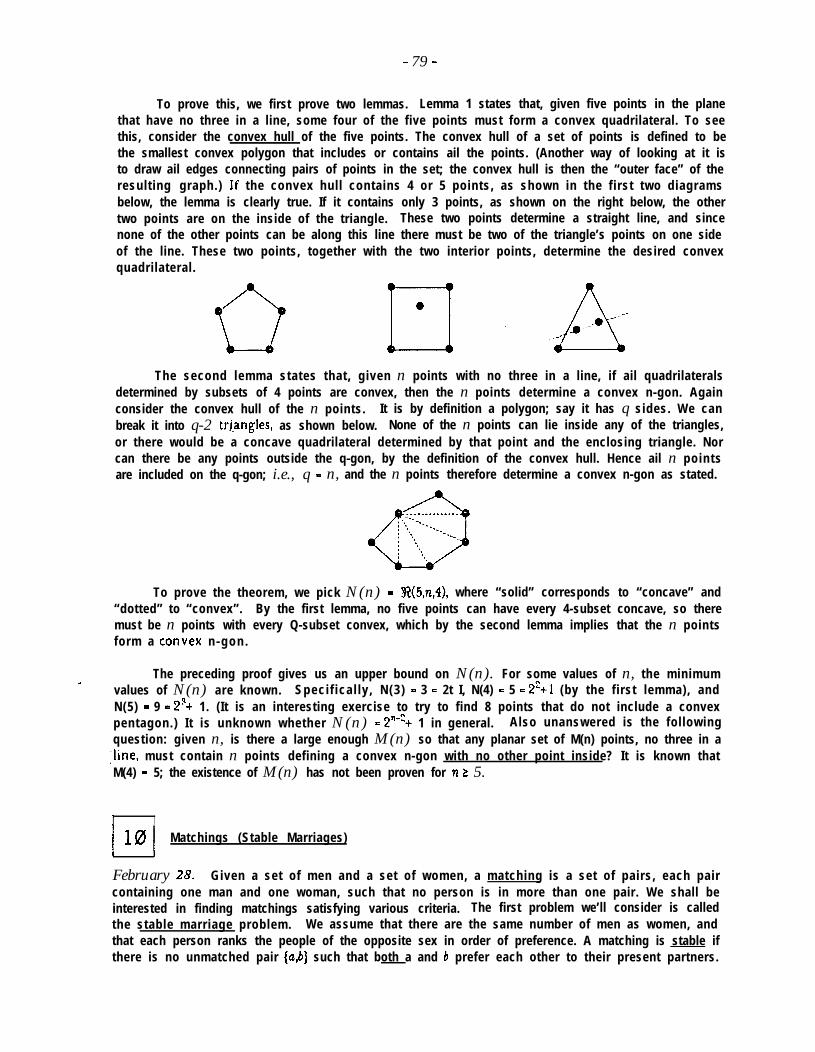
- 79 -

To prove this, we first prove two lemmas. Lemma 1 states that, given five points in the planethat have no three in a line, some four of the five points must form a convex quadrilateral. To seethis, consider the convex hull of the five points. The convex hull of a set of points is defined to bethe smallest convex polygon that includes or contains ail the points. (Another way of looking at it isto draw ail edges connecting pairs of points in the set; the convex hull is then the “outer face” of theresulting graph.) If the convex hull contains 4 or 5 points, as shown in the first two diagramsbelow, the lemma is clearly true. If it contains only 3 points, as shown on the right below, the othertwo points are on the inside of the triangle. These two points determine a straight line, and sincenone of the other points can be along this line there must be two of the triangle’s points on one sideof the line. These two points, together with the two interior points, determine the desired convexquadrilateral.

0 Aeo.---* -----___

The second lemma states that, given n points with no three in a line, if ail quadrilateralsdetermined by subsets of 4 points are convex, then the n points determine a convex n-gon. Againconsider the convex hull of the n points. It is by definition a polygon; say it has q sides. We canbreak it into q-2 trjangies, as shown below. None of the n points can lie inside any of the triangles,or there would be a concave quadrilateral determined by that point and the enclosing triangle. Norcan there be any points outside the q-gon, by the definition of the convex hull. Hence ail n pointsare included on the q-gon; i.e., q = n, and the n points therefore determine a convex n-gon as stated.

. . . . . . . . . . . . . .-_4’. --..-I .

0

‘,: .( --._ --: ‘, ---‘5 : ‘3

To prove the theorem, we pick N(n) = R(S,n,4), where “solid” corresponds to “concave” and“dotted” to “convex”. By the first lemma, no five points can have every 4-subset concave, so theremust be n points with every Q-subset convex, which by the second lemma implies that the n pointsform a con+ex n -gon.

The preceding proof gives us an upper bound on N(n). For some values of n, the minimum-values of N(n) are known. Speci f ica l ly , N(3) = 3 = 2t I, N(4) = 5 = 2% I (by the first lemma), andN(5) = 9 = 2% 1. (It is an interesting exercise to try to find 8 points that do not include a convexpentagon.) It is unknown whether N(n) = 2% 1 in general. Also unanswered is the followingquestion: given n, is there a large enough M(n) so that any planar set of M(n) points, no three in ailine, must contain n points defining a convex n-gon with no other point inside? It is known thatM(4) = 5; the existence of M(n) has not been proven for n L 5.

I I

I I10 Matchings (Stable Marriages)

February 25. Given a set of men and a set of women, a matching is a set of pairs, each paircontaining one man and one woman, such that no person is in more than one pair. We shall beinterested in finding matchings satisfying various criteria. The first problem we’ll consider is calledthe stable marriage problem. We assume that there are the same number of men as women, andthat each person ranks the people of the opposite sex in order of preference. A matching is stable ifthere is no unmatched pair {a,61 such that both a and 6 prefer each other to their present partners.

- 80 -

(If such a pair existed, they would run off together.) Although we speak of men and women, this isactually a rather facetious viewpoint; this problem is more often applied to relationships somewhatmore pragmatic than marriage, such as roommate assignments, dormitory room assignments, anduniversity admissions. Nevertheless, here we’ll discuss the problem in terms of marriages betweenmen and women.

For example, let’s designate the men with lower-case letters and the women with upper-case.Suppose the preference lists are as follows:

a: ABC A: batb: BAC B: cbac : ACB C: a c b

Suppose we take the matching {aB,bC,cAJ. Is this stable? No, because a prefers A over B, and Aprefers a over c, so a and A will run off together. Is there a stable matching for these people? Yes;here’s one: (aA,bB,cCj. In this matching, a and b have their top choices and therefore will not wantto run off with anyone else; c would prefer A, but A doesn’t prefer c. This matching is thereforestable. So is this one: {aC,bA,cBj. It turns out that, no matter what the people’s preferences are,there always exists at least one stable matching. We wish not only to prove this, but also to give amethod for finding one. (This is thus a case of constructive combinatorics.)

The method we’re about to present works something like this. The first man will propose tothe first woman on his list. She, having no better offer at this point, will accept. The second manwill then propose to his first choice, and so on. Eventually it may happen that a man proposes to awoman who already has a partner. She will compare the new offer to her current partner and willaccept whoever is higher on her list. The man she rejects will then go back to his list and proposeto his second choice, third choice, and so forth until he comes to a woman who accepts his offer. (Ifthis woman already had a partner, then the old partner gets rejected and he in turn starts proposingto women further down his list.) Eventually everything gets sorted out. Now let’s make this a bitmore formal.

A laorithm:

Each person starts out with no people “canceiled” from his or her list. People will becancelled from lists as the algorithm progresses.

For each man m, do propose(m), as defined below.

propose(m):Let W be the first uncancelled woman on m’s preference list.Do: refuse(PV,m), as defined below.

refuse(W,m):Let m’ be W’s current partner (if any).If W prefers m’ to m, then she rejects m, in which case:

(1) cancel m off W’s list and W off m’s list;(2) do: propose(m). (Now m must propose to someone else.)

Otherwise, W accepts m as her new partner, in which case:(1) cancel m’ off W’s list and W off m”s list;(2) do: propose( (Now m’ must propose to someone else.)

Let’s step through this algorithm using our earlier example. (This is the sort of thing bestdone at a blackboard, but we’ll see what we can do.) We first do propose(a). a’s top choice is A, so

-81 -

we do refuse(A,a). She has no current partner, so she accepts a. We proceed to the next man, b,whose first choice is B. She too accepts. Finally, we do propose(c), which in turn causes us to dorefuse(A,c). Since A’s current partner is IL, and she prefers a over c, she rejects c. We cross A off o fc’s list, and cross c off of A’s list, and do propose(c) again. This time, since A has been cancelledfrom his list, he proposes to C, who accepts. We have found a matching, and we have seen alreadythat this particular matching is stable.

Let’s look at a slightly more complex example. Consider the following preference lists.

a: DACB A: acdbb: ACDB B: dabcc : CDBA C: cbdad: D A C B D: bdca

Let’s step through the algorithm using these lists. First a proposes to D, who accepts. Then bproposes to A, who accepts, and c proposes to C, who accepts, Finally, n proposes to D, and the funbegins: D accepts n’s proposal and rejects a; a then proposes to A, who accepts a and rejects 6; bproposes to C, but C is happy and rejects him, so b next proposes to D. Now D rejects n in favor ofb, so d proposes to A . She rejects him, and he proposes to C, who also rejects him. Finally, lzproposes to B, who accepts. The final matching is: (aA,bD,cC,dB}. Note that someone can end upwith a despised paRner (B was n’s last choice) and the matching can still be stable. Note also thatthe algorithm can be run “the other way”, with the women proposing to the men. If we were to dothat in this particular example, we’d get the same solution with much less work.

Now let’s prove a few things about this algorithm. First of all, is it an algorithm? That is,does it necessarily terminate? Yes it does, because no man ever proposes twice to the same woman.Next, is a matching generated? Yes: once a woman has a partner, she always has one (she may“trade” for a better one, but she’ll never be without one). If there is an unmatched man, there mustalso be an unmatched woman. But an unmatched man will keep proposing until he has proposed toevery woma.n, so he must eventually propose to the unmatched woman, and she will accept. Soeveryone ends up in the matching.

Now we come to the interesting part- is the matching stable? Well, suppose it isn’t. Thenthere’s some pair, say aB, who are not matched to each other, such that each prefers the other overhis or her current partner. Let’s assume a is paired with A and B with b. So a prefers B to A and B

a prefers a to b. Since B appears ahead of A on a’s list, and a ended up proposing to A, we know thata must have proposed to B at some point. So why did B reject a ? The only reason for B to reject awould be if she were paired at that point with someone she preferred over a. But if this were thecase, she couldn’t possibly have ended up with b as her partner, since each woman’s partner can onlyimprove.

Next, we wish to show that the solution found by the algorithm is male optimal, i.e., that noman can do any better than he does in the matching found by the algorithm. Since each man endsup matched with the first woman on his list who hasn’t been cancelled, this is the same as sayingthat every time a woman W gets cancelled from a man m’s list, it implies that no stable matchingincludes the pair mW. Consider such a cancellation. W has proposals from m and m’, and sherejects m. Suppose the pair mW occurs in some stable matching. In this matching, m’ is paired withsome other woman, W’. If IV precedes W’ in m”s list, then m’ and W prefer each other over theirassigned partners, and the matching isn’t stable. Meanwhile, if W’ precedes W in m”s list, then W’was cancelled off m”s list by the algorithm, and so we have yet another cancellation that must be inour hypothetical matching. Since each cancelled pair included in the matching implies that anothersuch pair must also be in the matching, we have by induction that there must be an arbitrarily largenumber of pairs, cancelled by the algorithm, that are in this new matching. But that’s impossible,

- 82 -

because there aren’t an arbitrarily large number of men and women in the sets. Hence our initialassumption, that there was at least one cancelled pair mW that could occur in some stable matching,must be wrong. Hence the matching found by the algorithm is male optimal.

Finally, we wish to show that the solution found by the algorithm is female pessimal, i.e., thatno woman does worse in any other stable matching. Suppose some woman W is paired, in somestable matching S, with a man m' whom she ranks lower than the partner m assigned to her by thealgorithm. Then W prefers m over m'. But, by male optimality, the man m prefers W to whomeverhe gets in the matching S. Hence S is unstable.

Polya raised the question of whether there were any sort of global criteria of “goodness” whichcould be used to decide which of two matchings was “better”. Such a crrterion would presumablyrate any stable matching as being better than any unstable one, and would rate stable matchings thatwere female pessimal (or male pessimal) lower than stable matchings that were more “balanced”.Such a measurement would indeed be nice to have, but none such seems to exist in general. We’llget back to this issue later.

What about partial preference lists? That is, suppose that for each person there are somepeople they dislike so intensely that they’d rather remain single than be paired with those people. Inthis case there need not be a solution (obviously, since one person could refuse to marry anybody).Given a collection of partial preference lists, we wish to determine whether there is in fact a stablematching in which all the men and women are paired.

March 2. To solve this problem, we introduce one additional “dummy” man and one “dummy”woman. We’ll denote them by m and W, For each man, we add W at the end of his partial list,followecl by all the “real” women not already on his list. Similarly, we add m to each woman’s list,followed by all real men not on the list. We also create preference lists for the two dummies. T h eorder of the real men and women on these two lists is irrelevant; the only important feature is thatW is m’s !as~ choice, and m is W’s last choice. For instance, given the partial lists

a: DA A: acb: ACD B: d a bc: c c: cii: D A C B D: bdca

we would transform them into the following:

a : D A W B C A: acmbdb: A C D W B B: dabmcc : C W A B D C: cmabdd: D A C B W D: bdcamm A B C D W W: abcdm

By our earlier analysis we know that there must be a stable matching for this set of lists, since now.everybody lists a complete set of preferences. However, this stable matching might have someonematched to a person to whom he or she refuses to be married. We claim that there is a complete,stable matching for the original problem if and only if there is a stable matching for the newproblem in which m is paired with W .

Suppose we have a stable matching that includes the pair mW. Removing m and W can’tmake the matching unstable, since doing so can only reduce the number of possible alternatives foreveryone. So all we need show is that no person prefers being single over being paired with his orher partner. Suppose some man a prefers being single to being married to his partner, A. Then a

- 83 -

prefers W over A. But W prefers a to m, so this wasn’t really a stable matching to begin with. Thesame argument applies if there is some woman who would prefer being single. The “only if” part ofthe claim is trivial and is left as an exercise.

W e can go one step further and claim that, if some stable matching for the new problemincludes the pair mW, then they &l do. This follows directly from the male optimal solution, w h i c hwe can find using our algorithm. If this solution.includes the pair mW, then alJ stable matchings do,since m can’t do any better, and W was his last choice. On the other hand, if the male opt imalsolution doesn’t include mW, then no stable matching does, since this solution is female pessimal,implying that W can’t do worse than whomever she’s got in this matching.

Finally, suppose each person ranks all the others? (This is the sort of thing that might arisein, say, roommate assignments, since any person might be paired with any other.) For instance,consider the following preferences:

A: BCDB: ACDC: ADBD: CAB

which have the complete, stable matching: {AB,CD). Unfortunately, most of the results that weproved regarding the bipartite case (“bipartite” means that there were two independent sets, andeach pair included one element from each set) no longer apply. In particular, there need not be astable matching, and there is no efficient method known for finding one if it exists.

Tarjan assigned as homework the problem of finding a set of preference lists for four peoplesuch that there was no stable matching. This isn’t too difficult to do. Some people even managed toprove the uniqueness of the answer. Such a set of lists is the following:

A: BCDB: CADC: ABDD: (arbitrary)

Any set of lists of this form (that is, equivalent except for some interchanging of names) will haveno stable matching, and these are the only such lists for four people. (We won’t bother to prove thatahere.) There are 48 “unstable” sets of lists, out of a total of (3!)’ - 1296 possible sets.

I. I1 1 Matchings (Maximum Matchings)I IMarch 2. In the preceding section we mentioned the problem of coming up with a “global criterion”for deciding whether one matching is better than another, We noted that no such criterion appearsto exist in general. Nevertheless, there are some cases where a reasonably simple criterion suffices.For instance, if each possible pairing is either permitted or not permitted, with no other relativepreferences given, then we have no trouble. This is known as the maximum matching problem.

Stated precisely, the maximum matching problem is the following. (As in section 10, we’lldiscuss it in terms of men and women. A typical “real-life” application might involve assigningpeople to jobs. See also the “busing problem” mentioned on page 55.) We are given a set M of menand a set W of women. We are also given a set of “legal” pairs (a,b), where a is in M and b is in W.

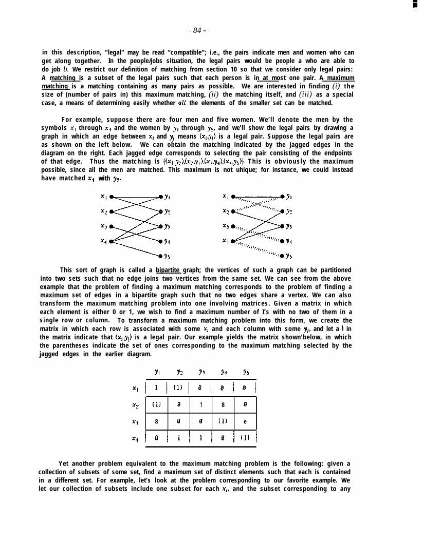
- 84 -

in this description, “legal” may be read “compatible”; i.e., the pairs indicate men and women who canget along together. In the people/jobs situation, the legal pairs would be people a who are able todo job b. We restrict our definition of matching from section 10 so that we consider only legal pairs:A matching is a subset of the legal pairs such that each person is in at most one pair. A maximummatching is a matching containing as many pairs as possible. We are interested in finding (i) t h esize of (number of pairs in) this maximum matching, (ii) the matching itself, and (iii) as a specialcase, a means of determining easily whether all the elements of the smaller set can be matched.

For example, suppose there are four men and five women. We’ll denote the men by thesymbols xl through x4 and the women by yl through y5, and we’ll show the legal pairs by drawing agraph in which an edge between x1 and yr means (x~J,) is a legal pair. Suppose the legal pairs areas shown on the left below. We can obtain the matching indicated by the jagged edges in thediagram on the right. Each jagged edge corresponds to selecting the pair consisting of the endpointsof that edge. Thus the matching is {(xl ,~~),(x~,~,),(x~,~~),(x.~,~~)~. Th is is obviously the maximumpossible, since all the men are matched. This maximum is not uhique; for instance, we could insteadhave matched x4 with ys.

This sort of graph is called a bipartite graph; the vertices of such a graph can be partitionedinto two sets such that no edge joins two vertices from the same set. We can see from the aboveexample that the problem of finding a maximum matching corresponds to the problem of finding amaximum set of edges in a bipartite graph such that no two edges share a vertex. We can alsotransform the maximum matching problem into one involving matrices. Given a matrix in whicheach element is either 0 or 1, we wish to find a maximum number of I’s with no two of them in asingle row or column. To transform a maximum matching problem into this form, we create thematrix in which each row is associated with some xi and each column with some yr, and let a 1 inthe matrix indicate that (zQ,$ is a legal pair. Our example yields the matrix shown’below, in whichthe parentheses indicate the set of ones corresponding to the maximum matching selected by thejagged edges in the earlier diagram.

YI Y2 Y.9 Y4 95

xi I l I( * I 0 I 8 I(1) 0 1 8 0

8 6 0 (1) e

Yet another problem equivalent to the maximum matching problem is the following: given acollection of subsets of some set, find a maximum set of distinct elements such that each is containedin a different set. For example, let’s look at the problem corresponding to our favorite example. Welet our collection of subsets include one subset for each xl, and the subset corresponding to any

- 85 -

par t icu lar x1 will consist of those y1 that form legal pairs with x1. Thus we have four subsets :etch], @i,~s], cr.,], and @Zl’ys,‘ysj. The maximum matching we’ve been us ing as a so lut ion in theprevious examples corresponds to selecting yZ from the first set, yI from the second, ys from thethird, and y5 from the fourth. When, as in this case, the selected elements include one from each set(as opposed to leaving some sets unrepresented), the set of elements selected is called a system ofdistinct representatives. This is often abbreviated to SDR.

Since all of these classes of problems- maximum matching, disjoint edges, matrix elementselection, and SDR-are equivalent (we haven’t actually shown that, but the transformations justdescribed can obviously be performed in either direction), a method for solving a.ny one of them canbe applied to get solutions to the others. So we’ll look at the problem of finding disjoint edges in abipartite graph. How do we go about finding the largest such set of edges? We start by defining afew more terms. We’ll use “matching” to refer to the set of edges selected, since any such selectioncorresponds to a matching in the original formulation of the problem.

A free vertex is one not contained in any edge of the matching. A path in a graph (we don’tseem to have defined this term before) is a sequence of edges u~z$, z$$, v~v.~, . . . , vk,tvk. (Whilewe’re at it, we’ll define a cycle (also called a circuit; we defined it informally on page 51) to be a pathin which the last vertex, vk’ is the same as the first, vI, We’ll be talking more about cycles later.) Apath is allowed to go through a vertex or vertices more than once; if it doesn’t it is called a simplepath. (Some texts use “path” and “walk” instead of “simple path” and “path”. We will occasionallyuse “path” to refer to a simple path when the non-repetition of vertices is obvious or unimportant.)Getting back to the problem at hand, we define an alternating path as a simple path consisting ofalternating matched and unmatched edges. If an alternating path connects two free vertices, it iscalled an augmenting path. If an augmenting path exists, the size of the matching can be increasedby one by switching the matched and unmatched edges along the path, as shown below. (As before,jagged edges indicate edges in the matching.)

augmenting path increased matchinga-* -dvvo-* -vv/‘*---~ awvv*-~vvve---l) vvv*

Note that we needn’t have restricted ourselves to simple paths, but if any vertex were repeated in anaugmenting path we could remove the cycle thus formed and still have an augmenting path, so it’seasier to consider only simple paths from the start.

This leads us to the following method for finding a maximum matching. This isn’t really ana algorithm, due to the vagueness of the second step.

Step I: Begin with any matching (e.g., the empty set).

Step 2: Look for an augmenting path. If one is found, increase the size of the matchingaccordingly. Repeat this step until no augmenting path is found.

We’ll ignore for the moment the problem of finding augmenting paths. First let’s prove that thismethod does indeed yield the maximum possible matching. Suppose it doesn’t; suppose the realmaximum is larger . Let M be a matching generated by the above method, and let MO be anym a x i m u m matchin

f. We’ll denote the size of M (the number of edges in M) by IMl. We want to

show that, if In-l1 < MJ, there must be an augmenting path in M.

We define M@&, by

M@Mo - (MUMf-J - (hIrIM&= (M-M(l) u o&dw’

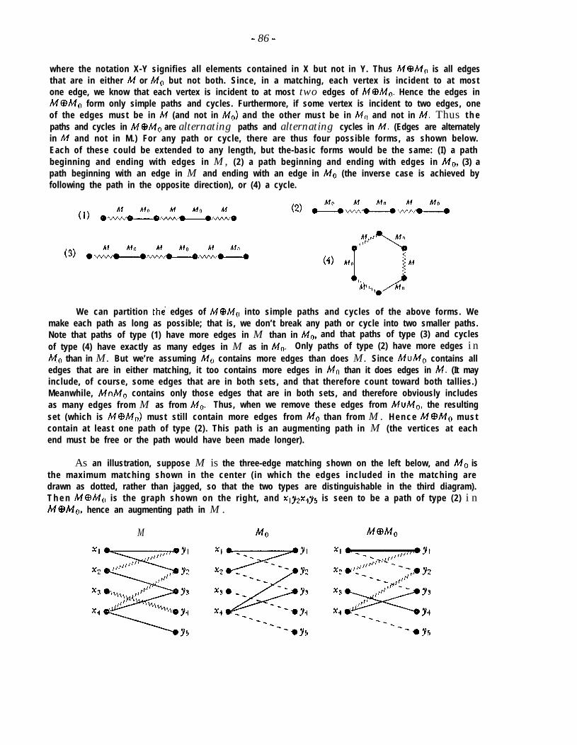
- 86 -

where the notation X-Y signifies all elements contained in X but not in Y. Thus M@MO is all edgesthat are in either M or M0 but not both. Since, in a matching, each vertex is incident to at mostone edge, we know that each vertex is incident to at most two edges of M@Mo. Hence the edges inM@Mo form only simple paths and cycles. Furthermore, if some vertex is incident to two edges, oneof the edges must be in M (and not in M,) and the other must be in M0 and not in M. Thus t h epaths and cycles in M$Mo are alternating paths and alternating cycles in M. (Edges are alternatelyin M and not in M.) For any path or cycle, there are thus four possible forms, as shown below.Each of these could be extended to any length, but the-basic forms would be the same: (I) a pathbeginning and ending with edges in M, (2) a path beginning and ending with edges in Mot (3) apath beginning with an edge in M and ending with an edge in MO (the inverse case is achieved byfollowing the path in the opposite direction), or (4) a cycle.

We can partition thi edges of M$&, into simple paths and cycles of the above forms. Wemake each path as long as possible; that is, we don’t break any path or cycle into two smaller paths.Note that paths of type (1) have more edges in M than in A&,, and that paths of type (3) and cyclesof type (4) have exactly as many edges in M as in MO. Only paths of type (2) have more edges i nM0 than in M. But we’re assuming MC, contains more edges than does M. Since MUM* contains alledges that are in either matching, it too contains more edges in MO than it does edges in M. (It mayinclude, of course, some edges that are in both sets, and that therefore count toward both tallies.)Meanwhile, MnMo contains only those edges that are in both sets, and therefore obviously includesas many edges from M as from MO. Thus, when we remove these edges from MUM,, the resultingset (which is M$Mo) must still contain more edges from MO than from M. H e n c e M@MO mustcontain at least one path of type (2). This path is an augmenting path in M (the vertices at eachend must be free or the path would have been made longer).

As an illustration, suppose M is the three-edge matching shown on the left below, and M. isthe maximum matching shown in the center (in which the edges included in the matching aredrawn as dotted, rather than jagged, so that the two types are distinguishable in the third diagram).T h e n M@Mo is the graph shown on the right, and qy2x4y~ is seen to be a path of type (2) i nM@Mo, hence an augmenting path in M .

M MO M@Mo

- 87 -

March 7 . Now that we’ve shown that the augment ing path method wi l l indeed f ind maximummatchings, let’s return to the question of how to find the augmenting paths. There is an algorithmfor doing this; it is called the labellinp: algorithm because it labels the men and women as they arereached via alternating paths. The labels indicate not only that the people have been reached, butalso where the path came from that reached them. The rules for labelling vertices of the graph areshown below. Labels are written inside brackets.

(i) Label any unlabelled free man with the label L-1, indicating the beginning of an alternatingpath.

(ii) If b is an unlabelled woman joined by an unmatched edge to a labelled man a, then label b with[al.

(iii) If a is an unlabelled man joined by a matched edge to a labelled woman b, then label a with Lb].

Notice that these rules take advantage of the bipartite nature of the graph. We’ll see later how theproblem becomes more difficult when the graph is not known to be bipartite. In the bipartite case,the labelling algorithm for finding augmenting paths is:

Apply the above labelling rules repeatedly until either(1) a free._woman is labelled, or(2) nothing more can be labelled.

In case (I), an augmenting path has been found, and the number of edges in the matchingcan be increased accordingly. (The path may be determined by tracing back through thelabels.) In case (2), there is no augmenting path and the matching is therefore maximum.

To see better how this algorithm works, let’s apply it to the non-maximum matching shown on theleft at the bottom of page 86. There is only one free man, namely xl, which by rule (i) is labelledr-1. Rule (ii) then permits us to label yI and y: with the label [x,1 (see leftmost diagram below). Byrule (iii) we can then label 3~: with [y,] and x4 with [y,J. At this point (center diagram below) wecould label yY with either 1~~1 or [x4] using rule (ii), or we could label y5 with [x~~J. We choose tolabel ys with [x,1; having labelled a free woman, we are done (rightmost diagram). We can find theaugmenting path by starting at the labelled free woman, y3, and looking at her label, which is [x4].We then look at q’s label, which is [y21. The label on yz, is [x1], and q’s label is L-1, indicating thebeginning of the path. The augmenting path is therefore x1y2x4yt\.

-[-IX,

x2

x3

x4

Y,k J

Y&I 1

Y&43

Y*l

Ys

If we increase the matching using this augmenting path, we get the matching shown on theleft on the following page. This matching is maximum, and if we try applying the algorithm it haltsimmediately, because there are no free men to be labelled using rule (i). We could also run thealgorithm “backwards”, treating the y’s as men and the x’s as women. In this case, we would label y5with l-1, and the algorithm would eventually finish with the graph labelled as shown on the right.Since nothing more can be labelled, and no free x has been labelled, the algorithm tells us thematching is maximum.

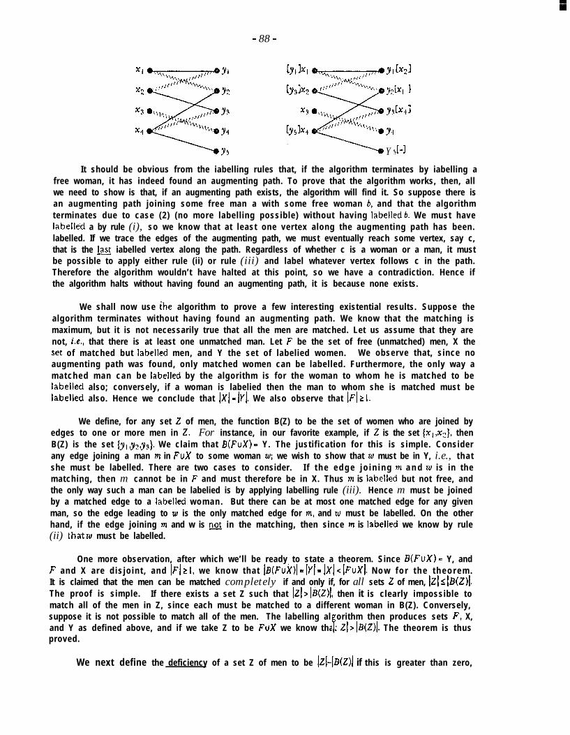
e

- 88 -

YIW

Y&Q 3

Y&d

Yl

Y sE-1It should be obvious from the iabelling rules that, if the algorithm terminates by iabelling a

free woman, it has indeed found an augmenting path. To prove that the algorithm works, then, allwe need to show is that, if an augmenting path exists, the algorithm will find it. So suppose there isan augmenting path joining some free man a with some free woman 6, and that the algorithmterminates due to case (2) (no more labell ing possible) without having labelled b. We must havelabelled a by rule (i), so we know that at least one vertex along the augmenting path has been.labelled. If we trace the edges of the augmenting path, we must eventually reach some vertex, say c,that is the & iabelled vertex along the path. Regardless of whether c is a woman or a man, it mustbe possible to apply either rule (ii) or rule (iii) and label whatever vertex follows c in the path.Therefore the algorithm wouldn’t have halted at this point, so we have a contradiction. Hence ifthe algorithm halts without having found an augmenting path, it is because none exists.

We shall now use the algorithm to prove a few interesting existential results. Suppose thealgorithm terminates without having found an augmenting path. We know that the matching ismaximum, but it is not necessarily true that all the men are matched. Let us assume that they arenot, i.e., that there is at least one unmatched man. Let F be the set of free (unmatched) men, X theset of matched but labelled men, and Y the set of labelied women. We observe that, since noaugmenting path was found, only matched women can be labelled. Furthermore, the only way amatched man can be labelled by the algorithm is for the woman to whom he is matched to belabelled also; conversely, if a woman is labelied then the man to whom she is matched must belabelled also. Hence we conclude that 1x1 - IYl. We also observe that IFI 2 I.

We define, for any set 2 of men, the function B(Z) to be the set of women who are joined byedges to one or more men in 2. For instance, in our favorite example, if 2 is the set (x1,x2>, thenB(Z) is the set {~~,,y~,y~}. We claim that B(FuX) - Y. The justification for this is simple. Considerany edge joining a man m in FuX to some woman zu; we wish to show that I(I must be in Y, i.e., thatshe must be labelled. There are two cases to consider. I f t h e e d g e j o i n i n g m a n d IU is in thematching, then m cannot be in F and must therefore be in X. Thus m is labelled but not free, andthe only way such a man can be labelied is by applying labelling rule (iii). Hence m must be joinedby a matched edge to a labelled woman. But there can be at most one matched edge for any givenman, so the edge leading to 10 is the only matched edge for M, and IU must be labelled. On the otherhand, if the edge joining m and w is pot in the matching, then since m is labelled we know by rule(ii) tha-t zu must be labelled.

One more observation, after which we’ll be ready to state a theorem. Since B(FuX) = Y, andF and X are d is jo int , and IFI L I, we know that IB(FuX)I = IY] - 1x1 < IFUX~. N o w f o r t h e t h e o r e m .It is claimed that the men can be matched completely if and only if, for all sets 2 of men, 1~1 I IB(z>~.The proof is simple. If there exists a set Z such that 1~1 > IB(z>~, then it is clearly impossible tomatch all of the men in Z, since each must be matched to a different woman in B(Z). Conversely,suppose it is not possible to match all of the men. The labelling al orithm then produces sets F, X,and Y as defined above, and if we take Z to be FuX we know that ZI > IB(z>~. The theorem is thus&proved.

We next define the deficiency of a set Z of men to be ~zI-IB(z)I if this is greater than zero,

- 89 -

and zero otherwise. The maximum deficiency is the maximum, taken over all sets Z of men, of thedeficiency of Z. We claim (here comes another theorem) that the size of a maximum matchingequals the number of men minus the maximum deficiency.

This theorem is obviously true if the maximum deficiency is zero, since in that case we knowfrom the previous theorem that we can get a complete matching. Also, since a set of men Z with apositive deficiency IzI-IB(z)I cannot have more than IBM of its men matched in any matching, it isclear that the size of a maximum matching must be less than or equal to the total number of menminus the maximum deficiency. We need only show that the size of the matching is also greaterthan or equal to the number of men minus the maximum deficiency; this will imply equality. Fromour earlier analysis we know that, in any maximum matching, IFUX~-~B(FUX)~ = <I~~+]xI)-IYI = IFI.Since the maximum deficiency is, by definition, at least as great as the deficiency of any particularset, we know that it is greater than or equal to IFUX~-~B(FUX>~ (since this is simply the deficiency ofthe set FuX). Hence the number of unmatched men (i.e., IFI) is less than or equal to the maximumdeficiency. The theorem follows.

A few pages back we defined what we meant by a system of distinct representatives (SDR).Since finding an SDR is equivalent to finding a complete matching, it makes sense that there shouldbe for SDRs a parallel to the theorem regarding complete matchings. This parallel theorem isknown as Hall’s Theorem, and it states that an SDR exists for a collection of subsets if and only if,for every k, any collection of k of the subsets contains at least k different elements. For example,suppose we look at-the SDR problem corresponding to the matching problem we’ve been using.There are four subsets, each of which consists of the women who are joined to a given man. Thesets are therefore @~,y:l, ~~,y~j, && and b2,yY,ys). It is easy to see that each set contains at leastone element, each pair of sets contains at least two different elements, and so on. Since the ith set isequiva lent to B({xJ), it is clear that Hall’s Theorem is equivalent to the theorem we’ve alreadyproven, which stated that a complete matching exists if and only if 1~1 ,< IBM for all sets of men Z.

Continuing the process of referencing the second previous theorem, Tarjan next presented acorollary to the theorem that related the size of a maximum matching to the maximum deficiency.The corollary states that, if every man is joined to at least k women, and every woman to at most kmen, then the men can be completely matched. To see this, we let Z be any set of men. Since eachman is joined to at least k women, there must be at least klZl edges coming from men in Z. To howmany different women do these edges lead? Each woman can account for at most k edges, so theremust be at least (klZl)+k women involved. Hence IBM > klZl+k = 1~1.

From the preceding corollary we can derive another, which we shall state without proof. (Theproof is trivial and is left as an exercise.) If there are fewer men than women, and each man isjoined to the same number of women, and each woman is joined to the same number of men, thenthe men can be completely matched.

We can use these results to prove Sperner’s Theorem, which we encountered in section 7(though we didn’t give it a name then). It concerned the problem of finding the largest collection ofsubsets of a given set, subject to the condition that none of the subsets should be a subset of anotherof the subsets. (In section 7 we used P6lya’s terminology and called such sets “disconnected”. Here,to avoid possible conflict with the term as it applies to graphs, we’ll switch to Tarjan’s terminologyand call the sets “incomparable”.) Sperner’s Theorem states that the maximum is achieved by takinghalf the size of the original set and letting the collection consist of all subsets of that size. Thusthere are (l,$J, subsets in the collection. For instance, if the original set is {a&c& it is not possibleto have more than (2, = 6 subsets without one of them being contained in another, and it is possibleto have exactly 6 such subsets, namely (a,b), (a,& (a,d), (b,c), (b,R}, and (c,n].

You wouldn’t expect maximum matchings to have any application to this problem, but it

- 90 -

turns out we can use some of the results we’ve just proven to prove Sperner’s Theorem. Thoughthis proof is non-trivial, it is considerably simpler than most (perhaps even all) other proofs of thetheorem. We shall consider any arbitrary collection of incomparable subsets and show that it can besystematically modified, without decreasing its size (i.e., the number of subsets), until it contains onlysubsets of size [n/2].

Let i be the size of the smallest subset, and let J be that of the largest. There are three cases(the first two are not mutually exclusive): (1) i < [n/Q, (2)j > [n/2], or (3) i = j = [n/2J. Supposei < Ln/2j. We construct a matching problem in which the “men” are all possible subsets of size i, the“women” are all possible subsets of size i+ I, and a set x of size i is joined by an edge to a set y ofsize i+ I if and only if x is a subset of y. We will show that there is a complete matching for the setsof size i; we can then replace each incomparable set of size i by its matching set of size i+ 1. In sodoing, we cannot affect the incomparability of the sets, since we are only increasing the size of thesmallest sets. (That is, adding an element to a set cannot make it a subset of another set, and thereare no smaller sets which could be subsets of this one.) How do we know that a complete matchingexists? Each set x of size i is joined to n-i sets of size i+l (one for each element not in x), while eachset y of size i+i is joined to it I sets of size i (one for each element in y). Since i < [n/2j, w h i c himplies i 5 (n- i)/2, we know that n-i 1 (nt I)/2 1 it I, so the first corollary from page 89 tells us thata complete matching must exist. (The second corollary could also be applied.) The casej > ln/2j ishandled similarly and is left as an exercise.

As homework, Tarjan assigned a problem involving what is called a system of simultaneousrepresentatives. Given a set S that has been partitioned into n subsets in two different ways, thus:

(where “lj” denotes the union of disjoint sets), a system of simultaneous representatives (SSR) is a setof n distinct elements xl, x2, . . . , x, that contains one element from each of the Ai and also containsone from each Bi. That is, the n elements form an SDR for the Ai, and the same n elements forman SDR for the Bi. The assignment was to prove that the following is a necessary and sufficientcondition for the existence of an SSR: for every k from I to n, no union of k of the A! is containedin the union of fewer than k of the Bt. For example, suppose S is the set (a,b,c,c&e& n = 3, t h eA-sets are (a,b), {c,n), and (ef), and the B-sets are (a&j, {dJ), and {e) . There is an SSR, namely(a,d,e). But if instead the B-sets w e r e {a,b,c,d), cfl, and (e), then there would be a union of twoA-sets, namely AIuAZ, that was contained in a single B-set, namely BI, so there would be no SSR.

This should have been a trivial assignment, but a remarkable number of students managed toturn it into an extremely complicated task. The necessity of the condition is easy to prove using anyof a number of approaches, but proving sufficiency by, say, induction can be quite tricky. Few ofthose who tried such an approach managed to come up with a valid proof. On the other hand,haven’t these people ever heard of the idea of using one result to prove another? We’ve proven anumber of theorems already; why should we have to start from scratch every time we want to proveanother result? Clearly, we shouldn’t. To prove that the above condition is necessary and sufficient,we construct a matching problem as follows. Let the “men” be the sets At, AZ, . . . , A,, and let the“women” be the sets B,, B:, . , . , 8,. T w o s e t s Ai and B, are a legal pair if and only if theirintersection AtnBj is not empty; i.e., the two sets have at least one element in common. If a completematching exists, then we can use it to construct an SSR by taking, for each pa.ir (Ai,Bj) in t h ematching, any element from A@ and placing it in the SSR. Since each of the A-sets and each o fthe B-sets occurs exactly once in a complete matching, this process yields n distinct elements formingan SDR both for the A-sets and for the B-sets. Conversely, suppose an SSR exists; we can use it tofind a complete matching. By definition, the SSR is a set of elements xl, xg, . . . , x, such that each3~~ is contained in a different AI from the others, and is also contained in a diffkrent B, from the

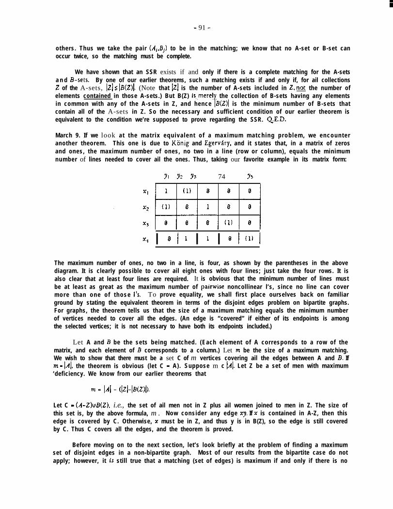
- 91 -

others. Thus we take the pair (Ai&,) to be in the matching; we know that no A-set or B-set canoccur twice, so the matching must be complete.

We have shown that an SSR exists if and only if there is a complete matching for the A-setsa n d B-sets. By one of our earlier theorems, such a matching exists if and only if, for ail collections2 of the A-sets, 121 s IB(Z)l. (Note that 1~1 is the number of A-sets included in 2, pot the number ofelements contained in those A-sets.) But B(Z) is..mereiy the collection of B-sets having any elementsin common with any of the A-sets in Z, and hence Ia(z)l is the minimum number of B-sets thatcontain all of the A-sets in Z. So the necessary and sufficient condition of our earlier theorem isequivalent to the condition we’re supposed to prove regarding the SSR. QED.

March 9. If we look at the matr ix equiva lent o f a maximum matching problem, we encounteranother theorem. This one is due to K6nig and Egerviry, and it states that, in a matrix of zerosand ones, the maximum number of ones, no two in a l ine (row or column), equals the minimumnumber of lines needed to cover ail the ones. Thus, taking our favorite example in its matrix form:

?I 7: 73 74 Y5

I 8 I l I l I 8 I(l)IThe maximum number of ones, no two in a line, is four, as shown by the parentheses in the abovediagram. It is clearly possible to cover ail eight ones with four lines; just take the four rows. It isalso clear that at least four lines are required. It is obvious that the minimum number of lines mustbe at least as great as the maximum number of pairwise noncollinear l’s, since no line can covermore than one of those 1’s. To prove equality, we shall first place ourselves back on familiarground by stating the equivalent theorem in terms of the disjoint edges problem on bipartite graphs.For graphs, the theorem tells us that the size of a maximum matching equals the minimum numberof vertices needed to cover all the edges. (An edge is “covered” if either of its endpoints is amongthe selected vertices; it is not necessary to have both its endpoints included.)

Let A and B be the sets being matched. (Each element of A corresponds to a row of thematrix, and each element of B corresponds to a column.) Let )~t be the size of a maximum matching.We wish to show that there must be a set C of m vertices covering ail the edges between A and B. If-m = 1~1, the theorem is obvious (let C = A). Suppose m c 1~1. Let Z be a set of men with maximum‘deficiency. We know from our earlier theorems that

m = I4 - <I4-llscmLet C = (A-Z)uB(Z), i.e., the set of ail men not in Z plus ail women joined to men in Z. The size ofthis set is, by the above formula, m . Now consider any edge xy. If x is contained in A-Z, then thisedge is covered by C. Otherwise, x must be in Z, and thus y is in B(Z), so the edge is still coveredby C. Thus C covers all the edges, and the theorem is proved.

Before moving on to the next section, let’s look briefly at the problem of finding a maximumset of disjoint edges in a non-bipartite graph. Most of our results from the bipartite case do notapply; however, it ts still true that a matching (set of edges) is maximum if and only if there is no

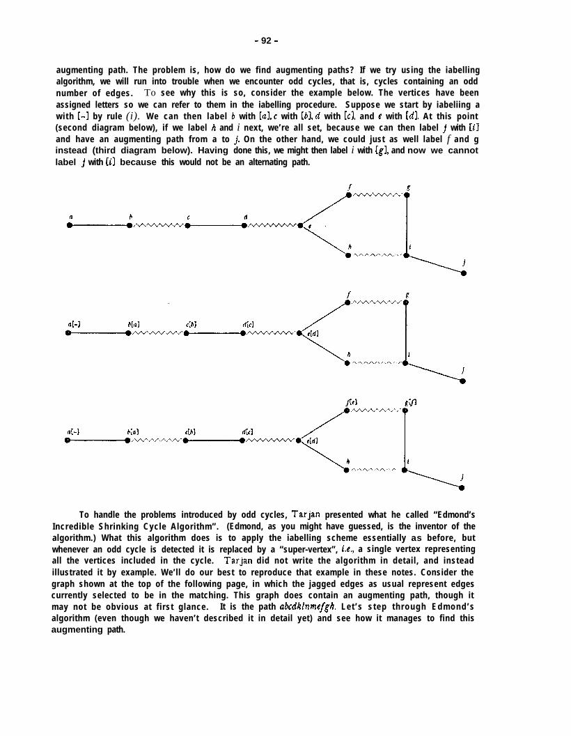
- 92 -

augmenting path. The problem is, how do we find augmenting paths? If we try using the iabellingalgorithm, we will run into trouble when we encounter odd cycles, that is, cycles containing an oddnumber of edges. To see why this is so, consider the example below. The vertices have beenassigned letters so we can refer to them in the iabelling procedure. Suppose we start by iabeliing awith [-I by rule (i). We can then label b with [al, c with E6J, n with EC], and e with Ml. At this point(second diagram below), if we label h and i next, we’re all set, because we can then label 1 with CiJand have an augmenting path from a to j. On the other hand, we could just as well label f and ginstead (third diagram below). Having done this, we might then label i with EgJ, and now we cannotlabel j with [iJ because this would not be an alternating path.

To handle the problems introduced by odd cycles, Tarjan presented what he called “Edmond’sIncredible Shrinking Cycle Algorithm”. (Edmond, as you might have guessed, is the inventor of thealgorithm.) What this algorithm does is to apply the iabelling scheme essentially as before, butwhenever an odd cycle is detected it is replaced by a “super-vertex”, i.e., a single vertex representingall the vertices included in the cycle. Tarjan did not write the algorithm in detail, and insteadillustrated it by example. We’ll do our best to reproduce that example in these notes. Consider thegraph shown at the top of the following page, in which the jagged edges as usual represent edgescurrently selected to be in the matching. This graph does contain an augmenting path, though itmay not be obvious at first glance. It is the path abcdklnmefgh. Let ’s s tep through Edmond’salgorithm (even though we haven’t described it in detail yet) and see how it manages to find thisaugmenting path.

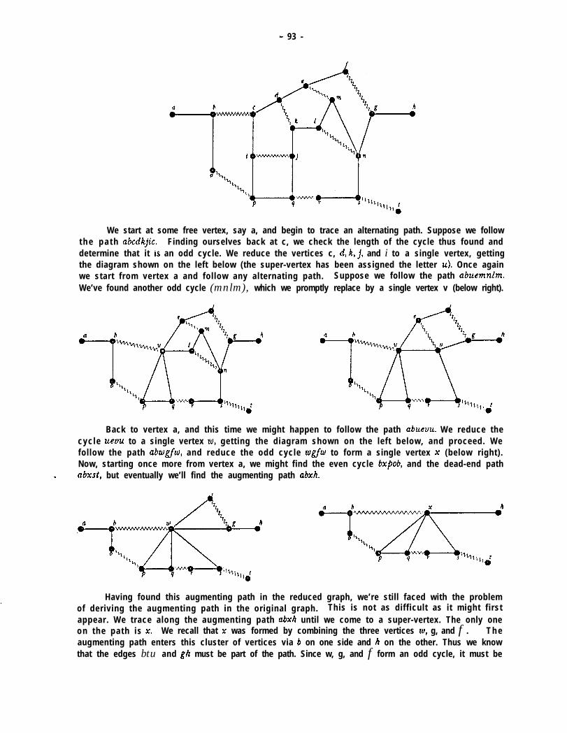
- 93 -

We start at some free vertex, say a, and begin to trace an alternating path. Suppose we followt h e p a t h abcdkjic. Finding ourselves back at c, we check the length of the cycle thus found anddetermine that it Is an odd cycle. We reduce the vertices c, n, k, j, and i to a single vertex, gettingthe diagram shown on the left below (the super-vertex has been assigned the letter IA). Once againwe start from vertex a and follow any alternating path. Suppose we follow the path abuemnlm.We’ve found another odd cycle (mnlm), which we promptly replace by a single vertex v (below right).

Back to vertex a, and this time we might happen to follow the path ubuevu. We reduce thecycle uevu to a single vertex ZU, getting the diagram shown on the left below, and proceed. Wefollow the path abrugfru, and reduce the odd cycle wgfru to form a single vertex x (below right).Now, starting once more from vertex a, we might find the even cycle bxpob, and the dead-end path

- abxsl, but eventually we’ll find the augmenting path abxh.

Having found this augmenting path in the reduced graph, we’re still faced with the problemof deriving the augmenting path in the original graph. This is not as difficult as it might firstappear. We trace along the augmenting path abxh until we come to a super-vertex. The only oneon the path is X. We recall that x was formed by combining the three vertices ru, g, and f. T h eaugmenting path enters this cluster of vertices via 6 on one side and h on the other. Thus we knowthat the edges btu and gh must be part of the path. Since w, g, and f form an odd cycle, it must be

- 94 -

possible to follow the cycle in one direction or the other to “link up” the path. It turns out that thedirection to follow is via f. So we have converted the path ab~h into the path abrufgh. We examinethis new path for super-vertices, and find w. We expand it to reintroduce the vertices u, e, and v,and find that b enters this cluster via the edge bu while f enters via ef. Again, there must be onedirection around the cycle forming an alternating path; it’s the direction that goes through v. Wenow have the path abuvefgh. Expanding u and v in similar fashion produces the augmenting pathwe want.

rl1 2 Network FlowI I

Network flow problems are usually stated in terms of directed graphs. A directed graph is the sameas the graphs we’ve been working with, except that each edge is assigned a direction. A nothercommon way of stating the distinction is that, whereas in an undirected graph each edge is a pair ofvertices, in a directed graph each edge is an ordered pair of vertices.

In a network flow problem, each edge has a capacity, indicating the maximum quantity (ofwhatever is flowing, such as oil or traffic) that can flow along that edge (in the direction of theedge). For instance, consider the graph below (left). The dotted lines will be explained later. Thedirection of the edges is indicated by arrows, and each edge is marked with its capacity. The vertexmarked J is called the source, and the vertex marked t is the sinkT h e s o u r c e i s a s s u m e d t o h a v eLan infinite supply of whatever it is that is flowing, and the sink has an infinite capacity. (It is easyto modify the graph (using additional vertices and edges) if we wish to impose limits on the sourceand sink, or have multiple sources and sinks, etc.) The objective of the network flow problem is tofind the maximum flow from the source to the sink subject to the conditions that (i) flow throughan edge must not exceed its capacity and (ii) flow at each vertex (except 3 and t) is conserved. Theflow out of J is, of course, equal to the flow into f. Either of these flows is called the value of theflow. In the example below, the maximum flow is 3 “units”,flow through the various edges be as shown on the right.

which can be achieved by letting the

A cut is a line or set of lines that completely severs ail connections between the source and thesink. Each of the two dotted lines shown in the diagram on the left above indicates a possible cut inthis network. The capacity of a cut is the sum of the capacities of all edges crossing the cut from thesource’s side to the sink?. Thus the capacities of the two cuts shown above are 4 (for the cut thatcrosses only two edges) and 3 (for the other, which crosses three “forward” edges and one “backward”edge; the backward edge is ignored). There is a classic theorem in network flow theory, which wasfirst formulated by Ford and Fuikerson. It is usually called the Max Flow Min Cut theorem, and itstates (appropriately enough) that the value of the maximum flow is equal to the capacity of theminimum cut As usual, we shall prove this theorem by constructing an algorithm, proving that itworks, and then using it to prove the theorem,

Once again we shall employ an augmenting scheme. Before describing it, let’s look at someexamples to get an idea as to what the augmenting paths look like. Suppose, in the example we’ve

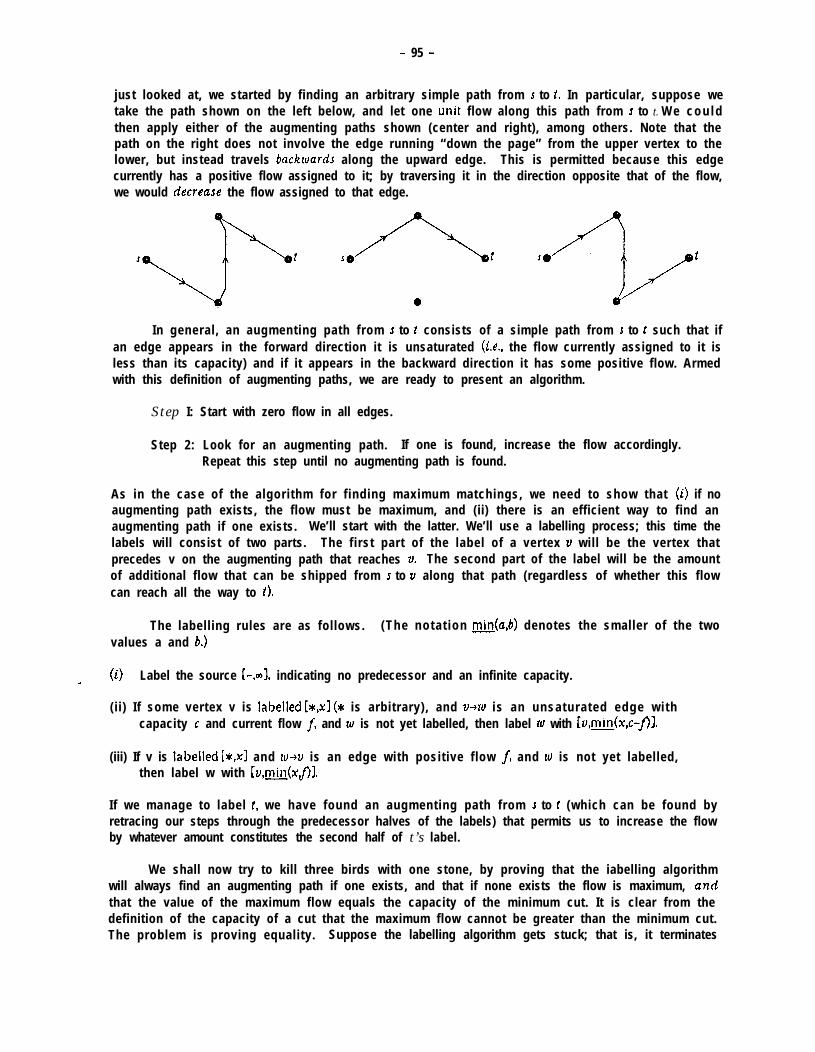
- 95 -

just looked at, we started by finding an arbitrary simple path from 5 to t. In particular, suppose wetake the path shown on the left below, and let one unit flow along this path from s to t. W e c o u l dthen apply either of the augmenting paths shown (center and right), among others. Note that thepath on the right does not involve the edge running “down the page” from the upper vertex to thelower, but instead travels bnckruar& along the upward edge. This is permitted because this edgecurrently has a positive flow assigned to it; by traversing it in the direction opposite that of the flow,we would decrease the flow assigned to that edge.

In general, an augmenting path from J to t consists of a simple path from J to t such that ifan edge appears in the forward direction it is unsaturated (i*e., the flow currently assigned to it isless than its capacity) and if it appears in the backward direction it has some positive flow. Armedwith this definition of augmenting paths, we are ready to present an algorithm.

Step I: Start with zero flow in all edges.

Step 2: Look for an augmenting path. If one is found, increase the flow accordingly.Repeat this step until no augmenting path is found.

As in the case of the algorithm for finding maximum matchings, we need to show that (i) if noaugmenting path exists, the flow must be maximum, and (ii) there is an efficient way to find anaugmenting path if one exists. We’ll start with the latter. We’ll use a labelling process; this time thelabels will consist of two parts. The first part of the label of a vertex 11 will be the vertex thatprecedes v on the augmenting path that reaches v. The second part of the label will be the amountof additional flow that can be shipped from J to v along that path (regardless of whether this flowcan reach all the way to t).

The labelling rules are as follows. (The notat ion n&(&,6) denotes the smaller of the twovalues a and 6.)

(i)- Label the source [-,~a], indicating no predecessor and an infinite capacity.

(i i) If some vertex v is labelled [x,x] (8 is arbitrary), and V-UU is an unsaturated edge wi thcapacity c and current flow J and zu is not yet labelled, then label w with [v,min(x,c-f)].

(iii) If v is labelled [*,x1 and zu+v is an edge with positive flow f, and IO is not yet labelled,then label w with [v,min(xf)].

If we manage to label t, we have found an augmenting path from 5 to t (which can be found byretracing our steps through the predecessor halves of the labels) that permits us to increase the flowby whatever amount constitutes the second half of t’s label.

We shall now try to kill three birds with one stone, by proving that the iabelling algorithmwill always find an augmenting path if one exists, and that if none exists the flow is maximum, am-lthat the value of the maximum flow equals the capacity of the minimum cut. It is clear from thedefinition of the capacity of a cut that the maximum flow cannot be greater than the minimum cut.The problem is proving equality. Suppose the labelling algorithm gets stuck; that is, it terminates

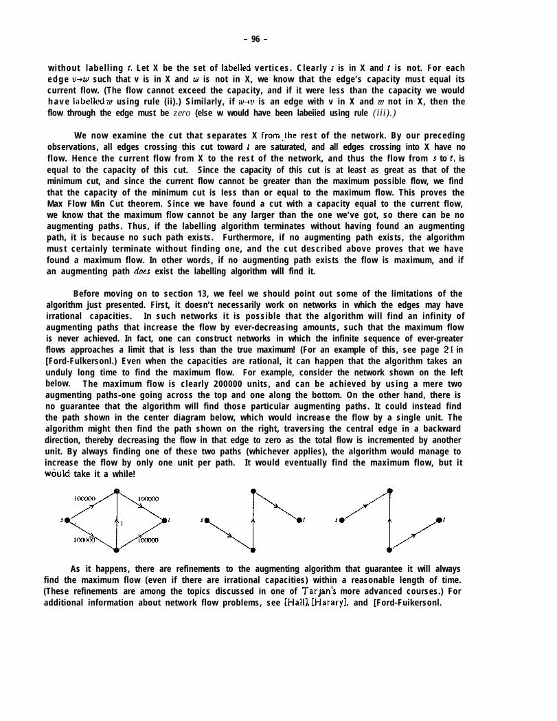
- 96 -

wi thout label l ing t. Let X be the set of labelled ver t ices. Clear ly s is in X and t is not. For eache d g e V-UU such that v is in X and IU is not in X, we know that the edge’s capacity must equal itscurrent flow. (The flow cannot exceed the capacity, and if it were less than the capacity we wouldh a v e labelled 1u using rule (ii).) Similarly, if IU+V is an edge with v in X and zu not in X, then theflow through the edge must be zero (else w would have been labeiied using rule (iii).)

We now examine the cut that separates X from.Jhe rest of the network. By our precedingobservations, all edges crossing this cut toward t are saturated, and all edges crossing into X have noflow. Hence the current flow from X to the rest of the network, and thus the flow from 5 to t, isequal to the capacity of this cut. Since the capacity of this cut is at least as great as that of theminimum cut, and since the current flow cannot be greater than the maximum possible flow, we findthat the capacity of the minimum cut is less than or equal to the maximum flow. This proves theMax Flow Min Cut theorem. Since we have found a cut with a capacity equal to the current flow,we know that the maximum flow cannot be any larger than the one we’ve got, so there can be noaugmenting paths. Thus, if the labelling algorithm terminates without having found an augmentingpath, it is because no such path exists. Furthermore, if no augmenting path exists, the algorithmmust certainly terminate without finding one, and the cut described above proves that we havefound a maximum flow. In other words, if no augmenting path exists the flow is maximum, and ifan augmenting path doe3 exist the labelling algorithm will find it.

Before moving on to section 13, we feel we should point out some of the limitations of thealgorithm just presented. First, it doesn’t necessarily work on networks in which the edges may haveirrational capacities. In such networks it is possible that the algorithm will f ind an infinity ofaugmenting paths that increase the flow by ever-decreasing amounts, such that the maximum flowis never achieved. In fact, one can construct networks in which the infinite sequence of ever-greaterflows approaches a limit that is less than the true maximum! (For an example of this, see page 21 in[Ford-Fulkersonl.) Even when the capacities are rational, it can happen that the algorithm takes anunduly long time to find the maximum flow. For example, consider the network shown on the leftbelow. The maximum flow is clearly 200000 units, and can be achieved by using a mere twoaugmenting paths-one going across the top and one along the bottom. On the other hand, there isno guarantee that the algorithm will find those particular augmenting paths. It could instead findthe path shown in the center diagram below, which would increase the flow by a single unit. Thealgorithm might then find the path shown on the right, traversing the central edge in a backwarddirection, thereby decreasing the flow in that edge to zero as the total flow is incremented by anotherunit. By always finding one of these two paths (whichever applies), the algorithm would manage toincrease the flow by only one unit per path. It would eventually find the maximum flow, but itw&id take it a while!

As it happens, there are refinements to the augmenting algorithm that guarantee it will alwaysfind the maximum flow (even if there are irrational capacities) within a reasonable length of time.(These refinements are among the topics discussed in one of Tarjan’s more advanced courses.) Foradditional information about network flow problems, see EI-Iaill, [Hararyl, and [Ford-Fuikersonl.

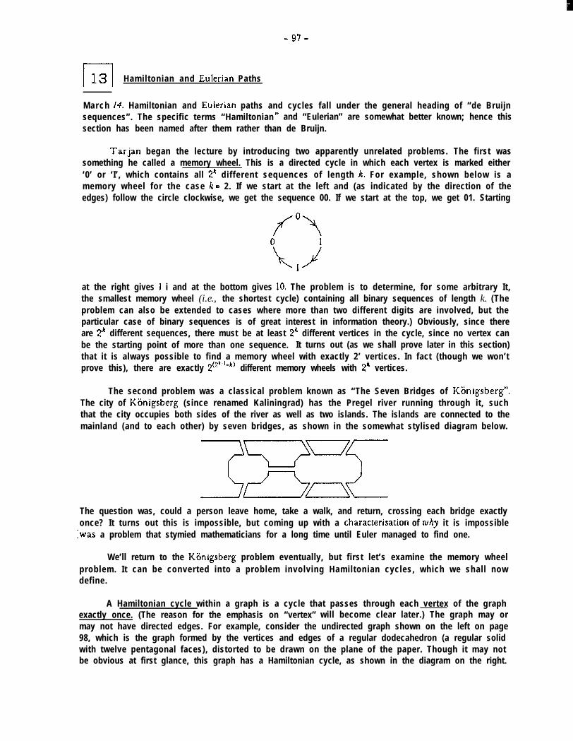
- 97 -

Hamiltonian and Eulerian Paths

March 24. Hamiltonian and Eulerian paths and cycles fall under the general heading of “de Bruijnsequences”. The specific terms “Hamiltonian ” and “Eulerian” are somewhat better known; hence thissection has been named after them rather than de Bruijn.

Tarjan began the lecture by introducing two apparently unrelated problems. The first wassomething he called a memory wheel. This is a directed cycle in which each vertex is marked either‘0’ or ‘I’, which contains all 2’ different sequences of length ic. For example, shown below is amemory wheel for the case k - 2. If we start at the left and (as indicated by the direction of theedges) follow the circle clockwise, we get the sequence 00. If we start at the top, we get 01. Starting

at the right gives I i and at the bottom gives 10. The problem is to determine, for some arbitrary It,the smallest memory wheel (i.e., the shortest cycle) containing all binary sequences of length k. (Theproblem can also be extended to cases where more than two different digits are involved, but theparticular case of binary sequences is of great interest in information theory.) Obviously, since thereare 2’ different sequences, there must be at least 2’ different vertices in the cycle, since no vertex canbe the starting point of more than one sequence. It turns out (as we shall prove later in this section)that it is always possible to find a memory wheel with exactly 2’ vertices. In fact (though we won’tprove this), there are exactly 2(2”-‘-k) different memory wheels with 2k vertices.

The second problem was a classical problem known as “The Seven Bridges of KSnigsberg”.The city of Kiinigsberg (since renamed Kaliningrad) has the Pregel river running through it, suchthat the city occupies both sides of the river as well as two islands. The islands are connected to themainland (and to each other) by seven bridges, as shown in the somewhat stylised diagram below.

The question was, could a person leave home, take a walk, and return, crossing each bridge exactlyonce? It turns out this is impossible, but coming up with a characterisation of ru@ it is impossible

Iwas a problem that stymied mathematicians for a long time until Euler managed to find one.

We’ll return to the Kiinigsberg problem eventually, but first let’s examine the memory wheelproblem. It can be converted into a problem involving Hamiltonian cycles, which we shall nowdefine.

A Hamiltonian cycle within a graph is a cycle that passes through each vertex of the graphexactly once. (The reason for the emphasis on “vertex” will become clear later.) The graph may ormay not have directed edges. For example, consider the undirected graph shown on the left on page98, which is the graph formed by the vertices and edges of a regular dodecahedron (a regular solidwith twelve pentagonal faces), distorted to be drawn on the plane of the paper. Though it may notbe obvious at first glance, this graph has a Hamiltonian cycle, as shown in the diagram on the right.

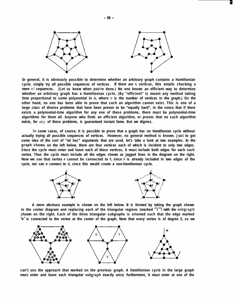
- 98 -

In general, it is obviously possible to determine whether an arbitrary graph contains a Hamiltoniancycle; simply try all possible sequences of vertices. If there are n vertices, this entails checking amere n! sequences. (Let us know when you’re done.) No one knows an efficient way to determinewhether an arbitrary graph has a Hamiltonian cycle, (By “efficient” is meant any method takingtime proportional to some polynomial in n, where n is the number of vertices in the graph.) On theother hand, no one has been able to prove that such an algorithm cannot exist. This is one of alarge class of diverse problems that have been proven to be “equally hard”, in the sense that if thereexists a polynomial-time algorithm for any one of these problems, there must be polynomial-timealgorithms for them all. Anyone who finds an efficient algorithm, or proves that no such algorithmexists, for any of these problems, is guaranteed instant fame. But we digress.-_

In some cases, of course, it is possible to prove that a graph has no Hamiltonian cycle withoutactually trying all possible sequences of vertices. However, no general method is known. Just to getsome idea of the sort of “ad hoc” arguments that are used, let’s take a look at two examples. In thegraph show n on the left below, there are four vertices each of which is incident to only two edges.Since the cycle must enter and leave each of these vertices, it must include both edges for each suchvertex. Thus the cycle must include all the edges shown as jagged lines in the diagram on the right.Now we see that vertex e cannot be connected to b, since b is already included in two edges of thecycle, nor can e connect to d, since this would create a non-Hamiltonian cycle.

A more abstruse example is shown on the left below. It is formed by taking the graph shownin the center diagram and replacing each of the triangular regions (marked “T”) with the subgraphshown on the right. Each of the three triangular subgraphs is oriented such that the edge marked‘*’ is connected to the vertex at the center of the graph. Note that every vertex is of degree 3, so we

can’t use the approach that worked on the previous graph. A Hamiltonian cycle in the large graphmust enter and leave each triangular subgraph exactly once; furthermore, it must enter at one of the

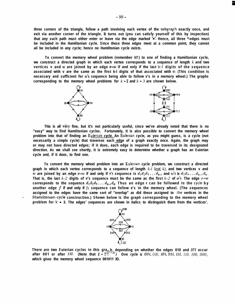
- 99 -

three corners of the triangle, follow a path involving each vertex of the subgraph exactly once, andexit via another corner of the triangle. It turns out (you can satisfy yourself of this by inspection)that any such path must either enter or leave via the edge marked ‘*‘. Hence, ail three *-edges mustbe included in the Hamiltonian cycle. Since these three edges meet at a common point, they cannotail be included in any cycle; hence no Hamiltonian cycle exists.

To convert the memory wheel problem (remember it?) to one of finding a Hamiltonian cycle,we construct a directed graph in which each vertex corresponds to a sequence of length k and twover t ices v and zu are joined by an edge v+w if and only if the last k-l d i g i t s o f t h e s e q u e n c eassociated with v are the same as the first k-l digits of that associated with W. (This condition isnecessary and sufficient for W’S sequence being able to follow v’s in a memory wheel.) The graphscorresponding to the memory wheel problems for k = 2 and k = 3 are shown below.

IO

00QI I

01

This is all v6ry fine, but it’s not particularly useful, since we’ve already noted that there is no“easy” way to find Hamiltonian cycles. Fortunately, it is also possible to convert the memory wheelproblem into that of finding an Eulerian cycle. An Eulerian cycle, as you might guess, is a cycle (notnecessarily a simple cycle) that traverses each edge of a graph exactly once. Again, the graph mayor may not have directed edges; if it does, each edge is required to be traversed in its designateddirection. As we shall see shortly, it is extremely easy to determine whether a graph has an Euieriancycle and, if it does, to find one.

To convert the memory wheel problem into an Eulerian cycle problem, we construct a directedgraph in which each vertex corresponds to a sequence of length k-l (not k), and two vertices v andw are joined by an edge V+YU if and only if U’S sequence is d,d& . . . dk-l and W’S is n$, . . . &-I&That is, the last k-2 digits of v’s sequence must be the same as the first k-2 of YU’S. The edge v+zucorresponds to the sequence d&& . . . &-l~k, T h u s a n e d g e e can be fo l lowed in the cycle b yanother edge f if and only if fs sequence can follow e’s in the memory wheel. (The sequencesassigned to the edges have the same sort of “overlap” as did those assigned to ,the vertices in the

- Ha.miltonian-cycle construction.) Shown below is the graph corresponding to the memory wheelproblem for k - 3. The edges’ sequences are shown in italics to distinguish them from the vertices’.

IO

00Cw?100 0 0 1

0 1 0

I+01

11001

011

I I111

There are two Euierian cycles in this gra h, depending on whether the edges 010 and 101 occurafter 0 0 1 or after 110. (Note that 2 = 2’ f ‘-‘-‘) .) One cycle is 001, OJO, 101, 011, 111, 110, 100, 000,which gives the memory wheel sequence 001011 IO.

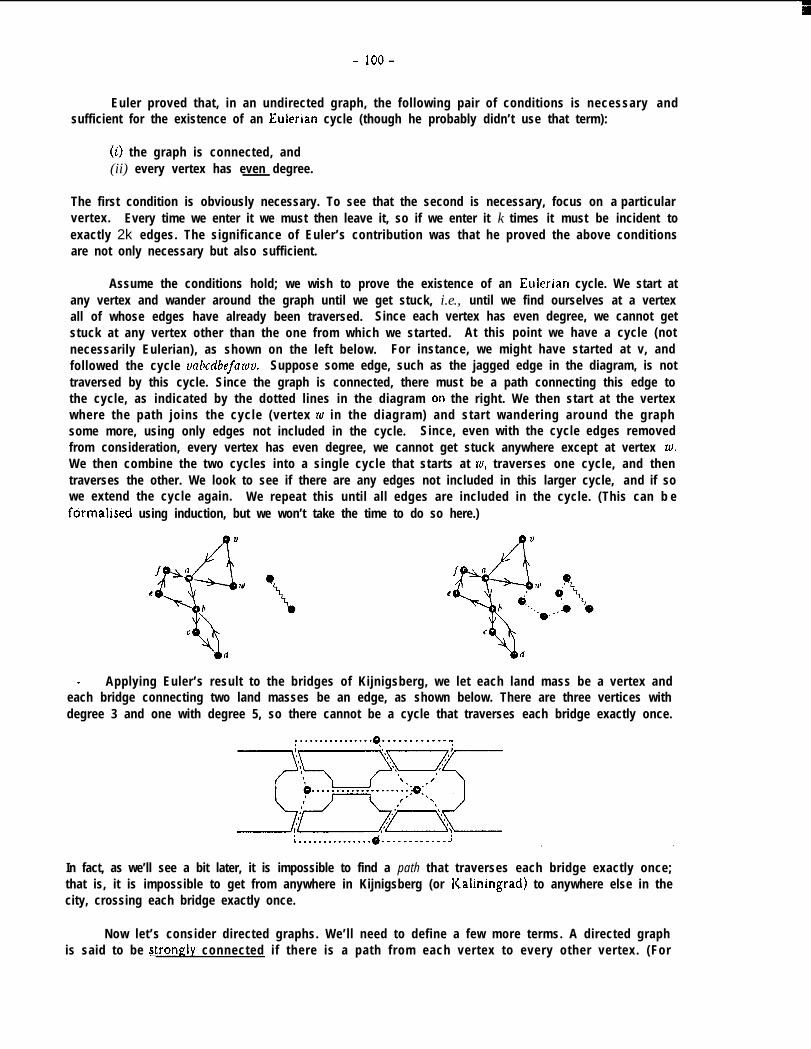
- loo-

Euler proved that, in an undirected graph, the following pair of conditions is necessary andsufficient for the existence of an Eulerian cycle (though he probably didn’t use that term):

(i) the graph is connected, and(ii) every vertex has even degree.

The first condition is obviously necessary. To see that the second is necessary, focus on a particularvertex. Every time we enter it we must then leave it, so if we enter it k times it must be incident toexactly 2k edges. The significance of Euler’s contribution was that he proved the above conditionsare not only necessary but also sufficient.

Assume the conditions hold; we wish to prove the existence of an Eulerian cycle. We start atany vertex and wander around the graph until we get stuck, i.e., until we find ourselves at a vertexall of whose edges have already been traversed. Since each vertex has even degree, we cannot getstuck at any vertex other than the one from which we started. At this point we have a cycle (notnecessarily Eulerian), as shown on the left below. For instance, we might have started at v, andfollowed the cycle vabcdbefaruv. Suppose some edge, such as the jagged edge in the diagram, is nottraversed by this cycle. Since the graph is connected, there must be a path connecting this edge tothe cycle, as indicated by the dotted lines in the diagram on the right. We then start at the vertexwhere the path joins the cycle (vertex zu in the diagram) and start wandering around the graphsome more, using only edges not included in the cycle. Since, even with the cycle edges removedfrom consideration, every vertex has even degree, we cannot get stuck anywhere except at vertex 10.We then combine the two cycles into a single cycle that starts at 10, traverses one cycle, and thentraverses the other. We look to see if there are any edges not included in this larger cycle, and if sowe extend the cycle again. We repeat this until all edges are included in the cycle. (This can b eformalised using induction, but we won’t take the time to do so here.)

- Applying Euler’s result to the bridges of Kijnigsberg, we let each land mass be a vertex andeach bridge connecting two land masses be an edge, as shown below. There are three vertices withdegree 3 and one with degree 5, so there cannot be a cycle that traverses each bridge exactly once.

In fact, as we’ll see a bit later, it is impossible to find a path that traverses each bridge exactly once;that is, it is impossible to get from anywhere in Kijnigsberg (or Kaliningrad) to anywhere else in thecity, crossing each bridge exactly once.

Now let’s consider directed graphs. We’ll need to define a few more terms. A directed graphis said to be stron& connected if there is a path from each vertex to every other vertex. (For

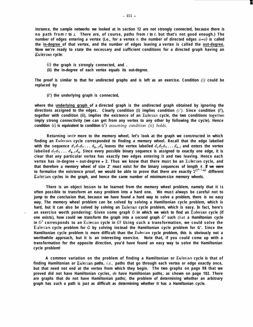
- 101 -

instance, the sample networks we looked at in section 12 are not strongly connected, because there isn o p a t h f r o m t to s. There are, of course, paths from J to t, but that’s not good enough.) Thenumber of edges entering a vertex (Le., for a vertex v, the number of directed edges WV) is calledthe in-degree of that vertex, and the number of edges leaving a vertex is called the out-degree.Now we’re ready to state the necessary and sufficient conditions for a directed graph having anEulerian cycle:

(i) the graph is strongly connected, and .(ii) the in-degree of each vertex equals its out-degree.

The proof is similar to that for undirected graphs and is left as an exercise. Condition (i) could bereplaced by

(i’) the underlying graph is connected,

where the underlying graph of a directed graph is the undirected graph obtained by ignoring thedirections assigned to the edges. Clearly condition (i) implies condition (i’). Since condition (i’),together with condition (ii), implies the existence of an Eulerian cycle, the two conditions togethelimply strong connectivity (we can get from any vertex to any other by following the cycle). Hencecondition (i) is equivalent to condition (i’) assuming condition (ii) holds.

Returning onle more to the memory wheel, let’s look at the graph we constructed in whichfinding an Eulerian cycle corresponded to finding a memory wheel. Recall that the edge labeliedwith the sequence +Q+, . . . n,-,n, leaves the vertex labeiled d&& . . . &,, and enters the vertexlabei ied && . . . &,dk. Since every possible binary sequence is assigned to exactly one edge, it isclear that any particular vertex has exactly two edges entering it and two leaving. Hence eachvertex has in-degree = out-degree c 2. Thus we know that there must be an Eulerian cycle, andthat therefore a memory wheel of size 2’ must exist for the binary sequences of length k. If we wereto formaiise the existence proof, we would be able to prove that there are exactly 2(“-‘-k) differentEulerian cycles in the graph, and hence the same number of minimum-size memory wheels.

There is an object lesson to be learned from the memory wheel problem, namely that it i soften possible to transform an easy problem into a hard one. We must always be careful not tojump to the conclusion that, because we have found a hard way to solve a problem, there is no easyway. The memory wheel problem can be solved by solving a Hamiltonian cycle problem, which ishard, but it can also be solved by solving an Eulerian cycle problem, which is easy. In fact, here’s

- an exercise worth pondering: Given some graph C in which we wish to find an Eulerian cycle (ifone exists), how could we transform the graph into a second graph C’ such .that a Hamiltonian cyclein G’ corresponds to an Eulerian cycle in G? Using such a t ransformat ion, we could solve theEulerian cycle problem for C by solving instead the Hamiltonian cycle problem for G’. Since theHamiltonian cycle problem is more difficult than the Eulerian cycle problem, this is obviously not aworthwhile approach, but it is an interesting exercise. Note that, if you could come up with atransformation for the opposite direction, you’d have found an easy way to solve the Hamiltoniancycle problem!

A common variation on the problem of f inding a Hamiltonian or Eulerian cycle is that o ffinding Hamiltonian or Eulerian paths, i.e., paths that go through each vertex or edge exactly once,but that need not end at the vertex from which they begin. The two graphs on page 98 that weproved did not have Hamiltonian cycles, no have Hamiltonian paths, as shown on page 102. Thereare graphs that do not have Hamiltonian paths; the problem of determining whether an arbitrarygraph has such a path is just as difficult as determining whether it has a Hamiltonian cycle.

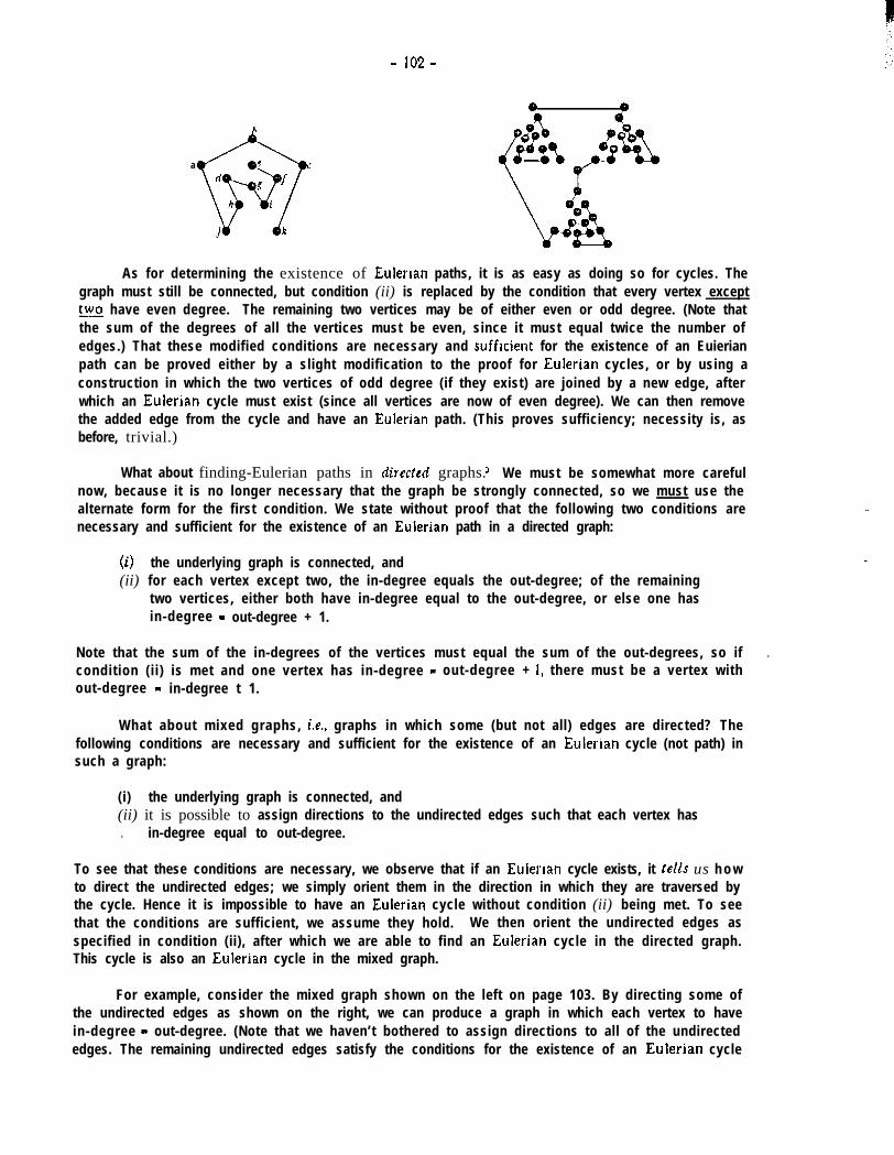
- 102-

a

As for determining the existence of Eulerian paths, it is as easy as doing so for cycles. Thegraph must still be connected, but condition (ii) is replaced by the condition that every vertex excepttwo have even degree. The remaining two vertices may be of either even or odd degree. (Note thatthe sum of the degrees of all the vertices must be even, since it must equal twice the number ofedges.) That these modified conditions are necessary and sufficient for the existence of an Euierianpath can be proved either by a slight modification to the proof for Eulerian cycles, or by using aconstruction in which the two vertices of odd degree (if they exist) are joined by a new edge, afterwhich an Eulerian cycle must exist (since all vertices are now of even degree). We can then removethe added edge from the cycle and have an Eulerian path. (This proves sufficiency; necessity is, asbefore, trivial.)

What about finding-Eulerian paths in directed graphs.7 We must be somewhat more carefulnow, because it is no longer necessary that the graph be strongly connected, so we must use thealternate form for the first condition. We state without proof that the following two conditions arenecessary and sufficient for the existence of an Eulerian path in a directed graph:

(i) the underlying graph is connected, and(ii) for each vertex except two, the in-degree equals the out-degree; of the remaining

two vertices, either both have in-degree equal to the out-degree, or else one hasin-degree = out-degree + 1.

Note that the sum of the in-degrees of the vertices must equal the sum of the out-degrees, so if .condition (i i) is met and one vertex has in-degree = out-degree + 1, there must be a vertex without-degree = in-degree t 1.

What about mixed graphs, i.e., graphs in which some (but not all) edges are directed? Thefollowing conditions are necessary and sufficient for the existence of an Eulerian cycle (not path) insuch a graph:

(i) the underlying graph is connected, and(ii) it is possible to assign directions to the undirected edges such that each vertex has

. in-degree equal to out-degree.

To see that these conditions are necessary, we observe that if an Eulerian cycle exists, it tell3 us h o wto direct the undirected edges; we simply orient them in the direction in which they are traversed bythe cycle. Hence it is impossible to have an Eulerian cycle without condition (ii) being met. To seethat the conditions are sufficient, we assume they hold. We then orient the undirected edges asspecified in condition (ii), after which we are able to find an Eulerian cycle in the directed graph.This cycle is also an Eulerian cycle in the mixed graph.

For example, consider the mixed graph shown on the left on page 103. By directing some ofthe undirected edges as shown on the right, we can produce a graph in which each vertex to havein-degree = out-degree. (Note that we haven’t bothered to assign directions to all of the undirectededges. The remaining undirected edges satisfy the conditions for the existence of an Eulerian cycle

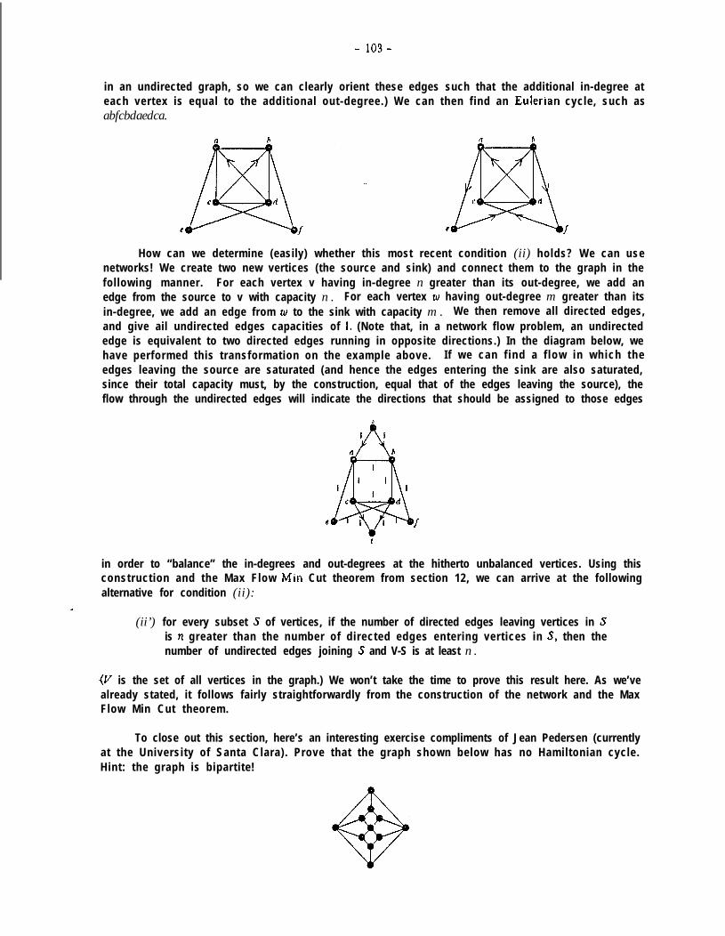
- 103-

in an undirected graph, so we can clearly orient these edges such that the additional in-degree ateach vertex is equal to the additional out-degree.) We can then find an Eulerian cycle, such asabfcbdaedca.

How can we determine (easily) whether this most recent condition (ii) holds? We can usenetworks! We create two new vertices (the source and sink) and connect them to the graph in thefollowing manner. For each vertex v having in-degree n greater than its out-degree, we add anedge from the source to v with capacity n . For each vertex w having out-degree m greater than itsin-degree, we add an edge from zu to the sink with capacity m . We then remove all directed edges,and give ail undirected edges capacities of 1. (Note that, in a network flow problem, an undirectededge is equivalent to two directed edges running in opposite directions.) In the diagram below, wehave performed this transformation on the example above. I f we can f ind a f low in which theedges leaving the source are saturated (and hence the edges entering the sink are also saturated,since their total capacity must, by the construction, equal that of the edges leaving the source), theflow through the undirected edges will indicate the directions that should be assigned to those edges

in order to “balance” the in-degrees and out-degrees at the hitherto unbalanced vertices. Using thisconstruction and the Max Flow Min Cut theorem from section 12, we can arrive at the followingalternative for condition (ii):

(ii’) for every subset S of vertices, if the number of directed edges leaving vertices in Sis n greater than the number of directed edges entering vertices in S, then thenumber of undirected edges joining S and V-S is at least n .

(V is the set of all vertices in the graph.) We won’t take the time to prove this result here. As we’vealready stated, it follows fairly straightforwardly from the construction of the network and the MaxFlow Min Cut theorem.

To close out this section, here’s an interesting exercise compliments of Jean Pedersen (currentlyat the University of Santa Clara). Prove that the graph shown below has no Hamiltonian cycle.Hint: the graph is bipartite!

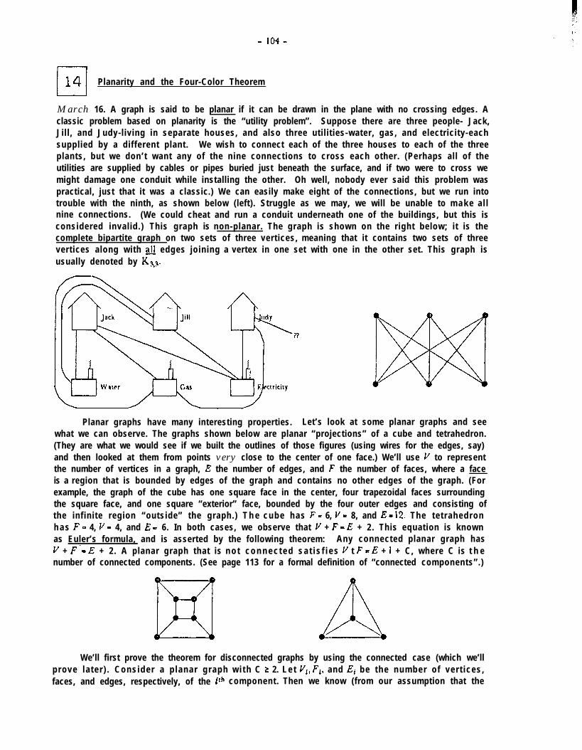
- 104-

cl14 Planarity and the Four-Color Theorem

March 16. A graph is said to be planar if it can be drawn in the plane with no crossing edges. Aclassic problem based on planarity is the “utility problem”. Suppose there are three people- Jack,Jil l , and Judy-living in separate houses, and also three util it ies-water, gas, and electricity-eachsupplied by a different plant. We wish to connect each of the three houses to each of the threeplants, but we don’t want any of the nine connections to cross each other. (Perhaps all of theutilities are supplied by cables or pipes buried just beneath the surface, and if two were to cross wemight damage one conduit while installing the other. Oh well, nobody ever said this problem waspractical, just that it was a classic.) We can easily make eight of the connections, but we run intotrouble with the ninth, as shown below (left). Struggle as we may, we will be unable to m a k e a l lnine connections. (We could cheat and run a conduit underneath one of the buildings, but this isconsidered invalid.) This graph is non-planar. The graph is shown on the right below; it is thecomplete bipartite graph on two sets of three vertices, meaning that it contains two sets of threevertices along with fi edges joining a vertex in one set with one in the other set. This graph isusually denoted by KI\,$.

Planar graphs have many interesting properties. Let’s look at some planar graphs and seewhat we can observe. The graphs shown below are planar “projections” of a cube and tetrahedron.(They are what we would see if we built the outlines of those figures (using wires for the edges, say)and then looked at them from points very close to the center of one face.) We’ll use V to representthe number of vertices in a graph, E the number of edges, and F the number of faces, where a faceis a region that is bounded by edges of the graph and contains no other edges of the graph. (Forexample, the graph of the cube has one square face in the center, four trapezoidal faces surroundingthe square face, and one square “exterior” face, bounded by the four outer edges and consisting ofthe infinite region “outside” the graph.) T h e cube has F = 6, V - 8, and E = 12. The tetrahedronh a s F - 4, V = 4, and E = 6. In both cases, we observe that V + F - E + 2. This equation is knownas Euler’s formula, and is asserted by the following theorem: Any connected planar graph hasV + F‘= E + 2. A planar graph that is n o t c o n n e c t e d s a t i s f i e s V t F = E + 1 + C, where C is t h enumber of connected components. (See page 113 for a formal definition of “connected components”.)

We’ll first prove the theorem for disconnected graphs by using the connected case (which we’llprove la ter ) . Consider a p lanar graph w i t h C L 2. L e t I$, F1, and Ei be the number of ver t ices ,faces, and edges, respectively, of the 1‘th component. Then we know (from our assumption that the

- 105-

theorem is true for connected graphs) that

v, + F, = E, + 2V, + F: = E:, t 2

..

and hence

(V,+Vz+ " ' +V,) + ( F , tF:+ ’ ’ ’ +Fc) = (E,+E:+ ’ ’ ’ +Ec) + 2 c .

C l e a r l y , (VI+Vz+ l . . +Vc) = V a n d (EltE2+ s l l +&) = E. When we sum the F1, however, we counteach interior face exactly once, but we count the exterior face C times. (The exterior face of adisconnected graph is an infinite region with two or more “holes” in it, one per component of thegraph. ) S ince F only counts this region once, we find that (FI+Fz+ l e a +Fc) = F + (C-l). Thus

v + F + ( C - l ) = E + 2c,

and the theorem follows.

Now we shart prove the theorem for connected graphs by induction on the number of edges.We start the induction by considering the graph with one vertex and no edges. (We cannot havemore than one vertex and no edges, since the graph is supposed to be connected.) This graph hasone face, namely the exterior face. So V = 1, F = 1, and E = 0. Since 1 + 1 = 0 + 2, the theoremholds. Now we perform the induction by seeing what happens when an edge is added to the graph.There are two cases: (1) the edge could lead to a vertex not previously included in the graph, or (2)the edge could join two old vertices. (The new edge cannot join two vertices neither of which wasyet in the graph, because this would result in a disconnected graph.)

In case (I), the new edge (the dotted edge in the diagram on the left below) does not create anynew faces. (The new edge becomes part of an existing face, the border of which includes both . I“sides” of the edge.) So if the graph prior to the addition of the dotted edge had V vertices, F faces,and E edges, then the graph including the dotted edge has V’ = V + I vertices, F’ = F faces, andE’ = E + I edges. By the induction hypothesis, we know that V + F = E + 2; hence we concludeV’ + F’ = V + 1 + F = E + 2 t I = E’ + 2. In case (2), the new edge divides an existing face into

- exactly two faces, as shown in the center diagram below. (The new edge cannot divide more thanone face without crossing another edge, as in the diagram on the right, and this is forbidden sincet h e g r a p h i s p l a n a r . ) T h e r e f o r e V’ = V, F’ = F t 1, a n d E ’ = E + 1, a n d w e a g a i n f i n d t h a t t h einduct ion hypothes is (V + F = E + 2) implies V’ + F’ = E’ t 2. The theorem is proved.

_--l!x

,I,’,,Note that, if we consider the boundaries of all the faces of a graph, each edge appears twice,

once for each “side” of the edge. In general each edge will appear in two different faces, but thereare exceptions. For example, consider the graph shown at the top of page 106. This graph hasthree faces: there are two triangular faces- abca and nefrl-and an exterior f a c e - a c d e f d c b a - w h i c h

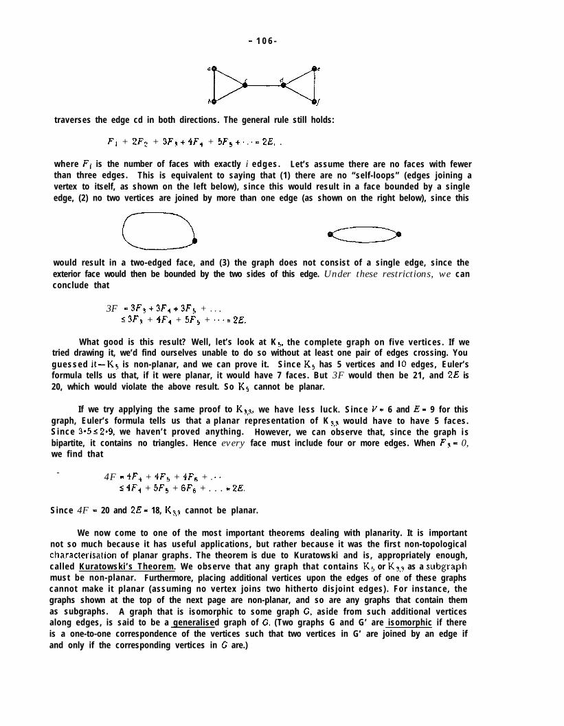
- 1 0 6 -

traverses the edge cd in both directions. The general rule still holds:

F, + 2F2 + 3F> t 4F., + 5F5 t m l a = 2E, .

where Fi is the number of faces with exactly i edges . Let’s assume there are no faces with fewerthan three edges. This is equivalent to saying that (1) there are no “self-loops” (edges joining avertex to itself, as shown on the left below), since this would result in a face bounded by a singleedge, (2) no two vertices are joined by more than one edge (as shown on the right below), since this

would result in a two-edged face, and (3) the graph does not consist of a single edge, since theexterior face would then be bounded by the two sides of this edge. Under these restrictions, we canconclude that

3F = 3F9 t 3F., t 3F5 + l l .6 3Fy + 4F., + 5FS + e -. e 2E.

What good is this result? Well, let’s look at K 5, the complete graph on five vertices. If wetried drawing it, we’d find ourselves unable to do so without at least one pair of edges crossing. Youguessed it-Kg is non-planar, and we can prove it. Since K5 has 5 vertices and 10 edges, Euler’sformula tells us that, if it were planar, it would have 7 faces. But 3F would then be 21, and 2E is20, which would violate the above result. So KI, cannot be planar.

If we try applying the same proof to Ks,s, we have less luck. Since V = 6 and E = 9 for thisgraph, Euler’s formula tells us that a planar representation of K 3,3 would have to have 5 faces.Since 3*5 ,< 2*9, we haven’t proved anything. However, we can observe that, since the graph i sbipartite, it contains no triangles. Hence every face must include four or more edges. When Fy - 0,we find that

4F = 4F., + 4FS + 4FG + l -.s 4F4 + 5F5 + 6FG + . . . = 2E.

Since 4F = 20 and 2E = 18, K3,s cannot be planar.

We now come to one of the most important theorems dealing with planarity. It is importantnot so much because it has useful applications, but rather because it was the first non-topologicalcharacterisation of planar graphs. The theorem is due to Kuratowski and is, appropriately enough,called Kuratowski’s Theorem. We observe that any graph that contains K1, or K9,y as a subgraphmust be non-planar. Furthermore, placing additional vertices upon the edges of one of these graphscannot make it planar (assuming no vertex joins two hitherto disjoint edges). For instance, thegraphs shown at the top of the next page are non-planar, and so are any graphs that contain themas subgraphs. A graph that is isomorphic to some graph G, aside from such additional verticesalong edges, is said to be a generalised graph of C. (Two graphs G and G’ are isomorphic if thereis a one-to-one correspondence of the vertices such that two vertices in G’ are joined by an edge ifand only if the corresponding vertices in C are.)

- 107-

Kuratowski’s Theorem states that euery n&-planar graph contains either a generalised K5 ora generalised K Y,s as a subgrap h. Generalised Ks’s and K Y,II’s are often referred to as Kuratowskisubgraphs. For example, consider the graph shown on the left below, which is known as “Petersen’sgraph”. This graph is non-planar, and so it must contain a Kuratowski subgraph. Indeed it does,as indicated in the diagram on the right. The graph is a generalised K3,3; the two sets of verticesforming the vertices of the bipartite graph are shown as dark and light circles, and the nine pathsforming the “edges” of the generalised graph are drawn solid (the remaining edges being dotted).

Unfortunately, the proof of Kuratowski’s Theorem is much too involved for us to attempt topresent in these notes. If you’re interested, you can find proofs in [Liu], pp. 212-220, and [Harary],pp. 109-l 12. The theorem is mathematically elegant but, as we have already noted, it is not veryuseful in practice. The most efficient algorithms for testing whether graphs are planar involveactually embedding the edges of the graphs in the plane. When such an algorithm determines thata given graph is non-planar, it is not necessarily clear how to go about isolating a Kuratowskisubgraph within that graph, although one is known to exist.

Returning to our earlier results, we can manipulate the formulas involving V, F, and E t ocome up with some additional theorems. For example, since V + F = E + 2 and 3F s 2E, we c a nconclude that

E + 2 s V + 2E/3

a and hence

E I 3V - 6.

This means that, given the restriction against one- and two-sided faces,,,no planar graph can have-more than 3V - 6 edges. Since, among V vertices, it is possible to have (0) = (V’-r/)/2 edges, this canbe interpreted as saying that planar graphs must have relatively few edges compared to most graphs.Note that K5 has E > 3V - 6, so we have again verified its non-planarity. If we know there are notriangular faces, the above result becomes E I 2V - 4, which verifies the non-planarity of Ks,Y.

We now look at a concept known as the dual of a planar graph. The dual is a graph thatconsists of one vertex for each face of the original graph, with edges connecting two vertices in thedual if and only if the corresponding faces shared an edge in the original graph. The diagram onthe following page shows the graph of the cube (dark circles and solid lines) together with its dual(white circles and dotted lines). Note that the dual is always itself planar, and that the dual of thedual is the original graph. We can set up a one-to-one correspondence between features of the twographs; each face in the original graph corresponds to a unique vertex in the dual, and vice versa,

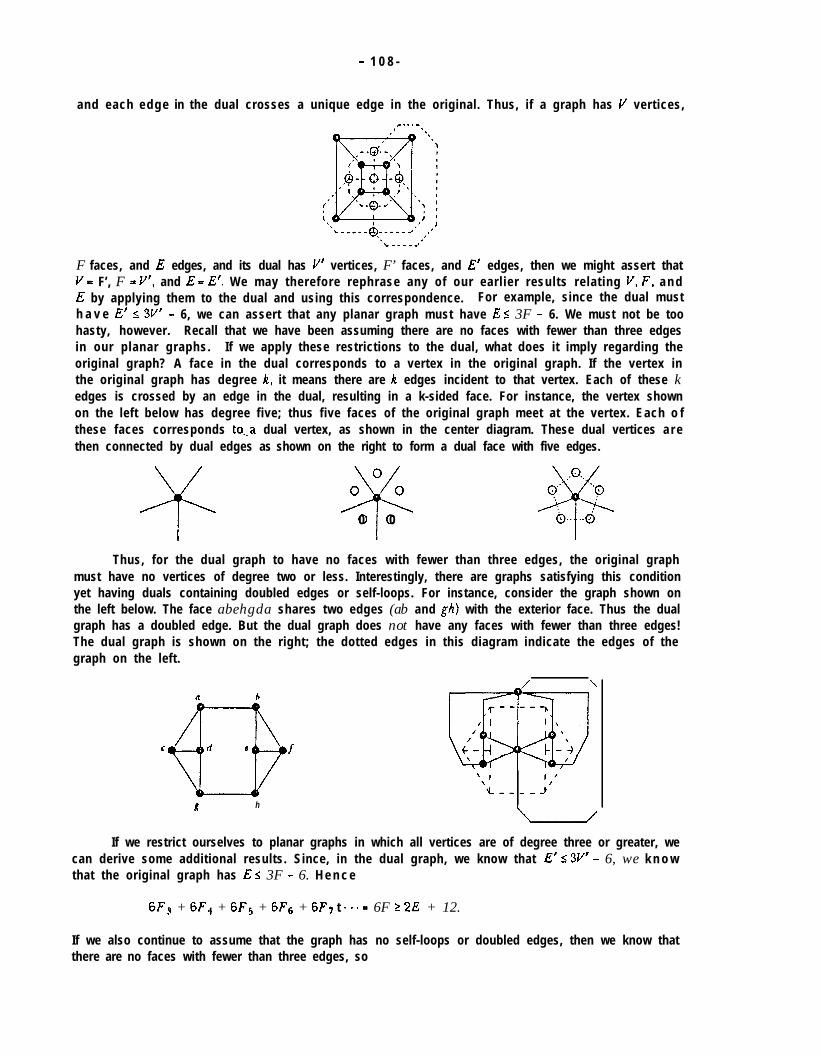
- 1 0 8 -

and each edge in the dual crosses a unique edge in the original. Thus, if a graph has V vertices,

F faces, and E edges, and its dual has V’ vertices, F’ faces, and E’ edges, then we might assert thatV I= F’, F = V’, and E = E’. We may therefore rephrase any of our earlier results relating V, F, a n dE by applying them to the dual and using this correspondence. For example, since the dual musth a v e E’ s 3V’ - 6, we can assert that any planar graph must have E I 3F - 6. We must not be toohasty, however. Recall that we have been assuming there are no faces with fewer than three edgesin our planar graphs. If we apply these restrictions to the dual, what does it imply regarding theoriginal graph? A face in the dual corresponds to a vertex in the original graph. If the vertex inthe original graph has degree k, it means there are k edges incident to that vertex. Each of these kedges is crossed by an edge in the dual, resulting in a k-sided face. For instance, the vertex shownon the left below has degree five; thus five faces of the original graph meet at the vertex. Each o fthese faces corresponds to--a dual vertex, as shown in the center diagram. These dual vertices a r ethen connected by dual edges as shown on the right to form a dual face with five edges.

00 0-?;‘-0 0

Thus, for the dual graph to have no faces with fewer than three edges, the original graphmust have no vertices of degree two or less. Interestingly, there are graphs satisfying this conditionyet having duals containing doubled edges or self-loops. For instance, consider the graph shown onthe left below. The face abehgda shares two edges (ab and gh) with the exterior face. Thus the dualgraph has a doubled edge. But the dual graph does not have any faces with fewer than three edges!The dual graph is shown on the right; the dotted edges in this diagram indicate the edges of thegraph on the left.

n h

6 h

If we restrict ourselves to planar graphs in which all vertices are of degree three or greater, wecan derive some additional results. Since, in the dual graph, we know that E’ s 3V’ - 6, we k n o wthat the original graph has E s 3F - 6. H e n c e

6F9 + 6F4 + 6F5 + 6F(j + 6F7 t ” ’ = 6F r 2E + 12.

If we also continue to assume that the graph has no self-loops or doubled edges, then we know thatthere are no faces with fewer than three edges, so

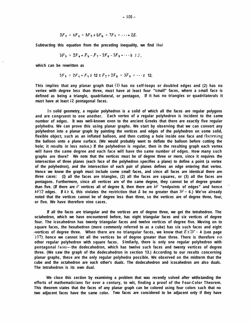
- 109-

3Fy + 4F4 + 5F5 + 6FG + 7F, + qm. = 2E.

Subtracting this equation from the preceding inequality, we find that

3Fy + 2F4 t F5 - F7 - 2F8 - 3F9 - 0 0. r 1 2 ,

which can be rewritten as

3F9 + 2F, -I- F5 2 12 t F7 + 2Fs + 3Fg + a 0. r 12.

This implies that any planar graph that (I) has no self- loops or doubled edges and (2) has novertex with degree less than three, must have at least four “small” faces, where a small face isdefined as being a triangle, quadrilateral, or pentagon, If it has no triangles or quadrilaterals itmust have at least 12 pentagonal faces.

In solid geometry, a regular polyhedron is a solid of which all the faces are regular polygonsand are congruent to one another. Each vertex of a regular polyhedron is incident to the samenumber of edges. It was well-known even to the ancient Greeks that there are exactly five regularpolyhedra. We can prove this using planar graphs. We start by observing that we can convert anypolyhedron into a planar graph by painting the vertices and edges of the polyhedron on some solid,flexible object, such as an inflated balloon, and then cutting a hole inside one face and fla.tteningthe balloon onto a plane surface. (We would probably want to deflate the balloon before cutting thehole; it results in less noise.) If the polyhedron is regular, then in the resulting graph each vertexwill have the same degree and each face will have the same number of edges. How many suchgraphs are there? We note that the vertices must be of degree three or more, since it requires theintersection of three planes (each face of the polyhedron specifies a plane) to define a point (a vertexof the polyhedron), and the intersection of each pair of planes defines an edge entering that vertex.Hence we know the graph must include some small faces, and since all faces are identical there arethree cases: (I) all the faces are triangles, (2) all the faces are squares, or (3) all the faces arepentagons. Furthermore, since all vertices are of the same degree, they cannot be of degree greaterthan five. (If there are I/ vertices all of degree It, then there are kV “endpoints of edges” and hence ’&V/2 edges. If k 2 6, this violates the restriction that E be no greater than 3V - 6.) We’ve alreadynoted that the vertices cannot be of degree less than three, so the vertices are of degree three, four,or five. We have therefore nine cases.

If all the faces are triangular and the vertices are of degree three, we get the tetrahedron. Theoctahedron, which we have encountered before, has eight triangular faces and six vertices of degreefour. The icosahedron has twenty triangular faces and twelve vertices of degree five. Moving on tosquare faces, the hexahedron (more commonly referred to as a cube) has six such faces and eight-vertices of degree three. When there are no triangular faces, we know that E I 2V - 4 (see page-10’7); hence we cannot let all the vertices be of degree greater than three. There is therefore noother regular polyhedron with square faces. Similarly, there is only one regular polyhedron withpentagonal faces- the dodecahedron, which has twelve such faces and twenty vertices of degreethree. (We saw the graph of the dodecahedron in section 13.) According to our results concerningplanar graphs, these are the only regular polyhedra possible. We observed on the midterm that thecube and the octahedron are each other’s duals. The dodecahedron and icosahedron are also duals.The tetrahedron is its own dual.

We close this section by examining a problem that was recently solved after withstanding theefforts of mathematicians for over a century, to wit, f inding a proof of the Four-Color Theorem.This theorem states that the faces of any planar graph can be colored using four colors such that notwo adjacent faces have the same color. Two faces are considered to be adjacent only if they have

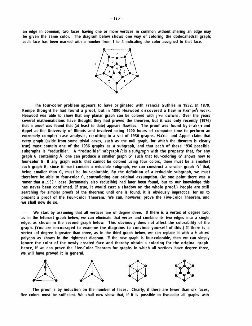
- IIO-

an edge in common; two faces having one or more vertices in common without sharing an edge maybe given the same color. The diagram below shows one way of coloring the dodecahedral graph;each face has been marked with a number from 1 to 4 indicating the color assigned to that face.

The four-color problem appears to have originated with Francis Guthrie in 1852. In 1879,Kempe thought he had found a proof, but in 1890 Heawood discovered a f law in Kempe’s work .Heawood was able to show that any planar graph can be colored with five colors. Over the yearsseveral mathematicians have thought they had proved the theorem, but it was only recently (1976)that a proof was found that (at least to date) appears flawless. The proof was found by Haken andAppel at the University of Illinois and involved using 1200 hours of computer time to perform anextremely complex case analysis, resulting in a set of 1936 graphs. Haken and Appel claim thatevery graph (aside from some trivial cases, such as the null graph, for which the theorem is clearlytrue) must contain one of the 1936 graphs as a subgraph, and that each of these 1936 possiblesubgraphs is “reducible”. A “reducib le” subgraph R is a subgraph with the property that, for anygraph G containing R, one can produce a smaller graph G’ such that four-coloring G’ shows how tofour-color G. If any graph exists that cannot be colored using four colors, there must be a smallestsuch graph G; since it must contain a reducible subgraph, we can construct a smaller graph G’ that,being smaller than G, must be four-colorable. By the definition of a reducible subgraph, we musttherefore be able to four-color C, contradicting our original assumption. (At one point there was arumor that a 193’7th case (fortunately also reducible) had later been found, but to our knowledge thishas never been confirmed. If true, it would cast a shadow on the whole proof.) People are stil lsearching for simpler proofs of the theorem; until one is found, it is obviously impractical for us topresent a proof of the Four-Color Theorem. We can, however, prove the Five-Color Theorem, andwe shall now do so.

- We start by assuming that all vertices are of degree three. If there is a vertex of degree two,as in the leftmost graph below, we can eliminate that vertex and combine its two edges into a singleedge, as shown in the second graph below. This obviously does not affect the colorability of thegraph. (You are encouraged to examine the diagrams to convince yourself of this.) If there is avertex -of degree k greater than three, as in the third graph below, we can replace it with a k-sidedpolygon as shown in the rightmost diagram. If the new graph is four-colorable, then we can simplyignore the color of the newly created face and thereby obtain a coloring for the original graph.Hence, if we can prove the Five-Color Theorem for graphs in which all vertices have degree three,we will have proved it in general.

The proof is by induction on the number of faces. Clearly, if there are fewer than six faces,five colors must be sufficient. We shall now show that, if it is possible to five-color all graphs with

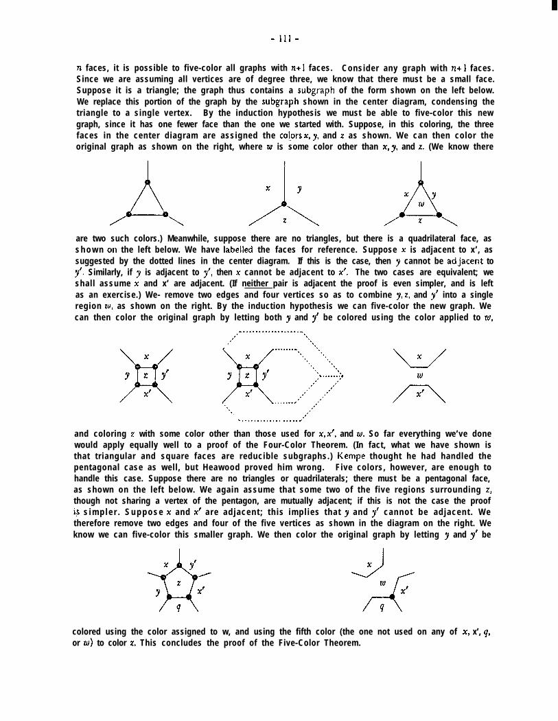
- Ill-

n faces, it is possible to five-color all graphs with nt 1 faces. Consider any graph with 72+1 faces.Since we are assuming all vertices are of degree three, we know that there must be a small face.Suppose it is a triangle; the graph thus contains a subgraph of the form shown on the left below.We replace this portion of the graph by the subgraph shown in the center diagram, condensing thetriangle to a single vertex. By the induction hypothesis we must be able to five-color this newgraph, since it has one fewer face than the one we started with. Suppose, in this coloring, the threefaces in the center diagram are assigned the co@-s X, y, and r as shown. We can then color theoriginal graph as shown on the right, where zu is some color other than x, y, and z. (We know there

are two such colors.) Meanwhile, suppose there are no triangles, but there is a quadrilateral face, ass h o w n on the left below. We have labelled the faces for reference. Suppose x is adjacent to x’, assuggested by the dotted lines in the center diagram. If this is the case, then y cannot be adja.cent toy’. Similarly, if y is adjacent to y’, then x cannot be adjacent to 3~‘. The two cases are equivalent; weshall assume x and x’ are adjacent. (If neither pair is adjacent the proof is even simpler, and is leftas an exercise.) We- remove two edges and four vertices so as to combine y, z, and y’ into a singleregion 10, as shown on the right. By the induction hypothesis we can five-color the new graph. Wecan then color the original graph by letting both y and y’ be colored using the color applied to IU,

x /xiY 2! Y’x’ \

A

.I.x

Y 2 Y’

x’. . .-. ‘.

. . . . . . . . . . . . . . .-...d

and coloring 2 with some color other than those used for X, x’, and ZU. So far everything we’ve donewould apply equally well to a proof of the Four-Color Theorem. (In fact, what we have shown isthat triangular and square faces are reducible subgraphs.) Kempe thought he had handled thepentagonal case as well, but Heawood proved him wrong. Five colors, however, are enough tohandle this case. Suppose there are no triangles or quadrilaterals; there must be a pentagonal face,as shown on the left below. We again assume that some two of the five regions surrounding 2,though not sharing a vertex of the pentagon, are mutually adjacent; if this is not the case the proofis s i m p l e r . S u p p o s e x and x’ are adjacent ; th is impl ies that y and y’ cannot be adjacent . Wetherefore remove two edges and four of the five vertices as shown in the diagram on the right. Weknow we can five-color this smaller graph. We then color the original graph by letting y and y’ be

colored using the color assigned to w, and using the fifth color (the one not used on any of X, x’, q,or zu) to color z. This concludes the proof of the Five-Color Theorem.

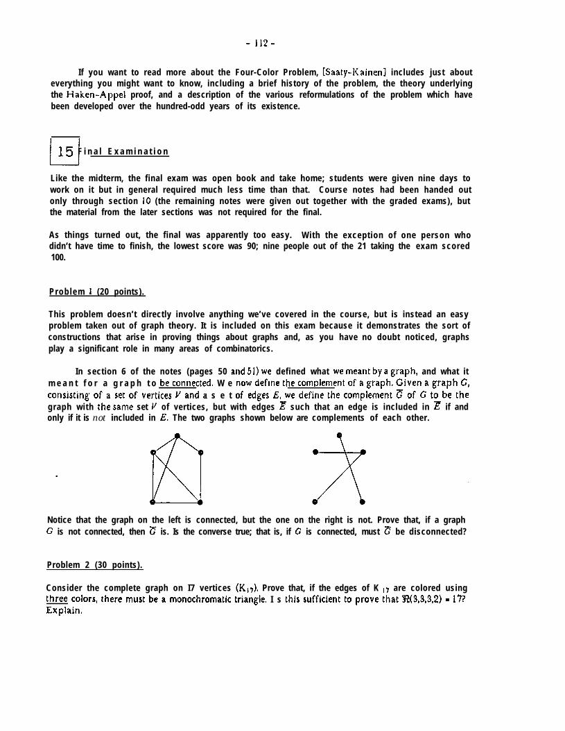
- 112-

If you want to read more about the Four-Color Problem, [Saaty-Kainenl includes just abouteverything you might want to know, including a brief history of the problem, the theory underlyingthe Haken-Appel proof, and a description of the various reformulations of the problem which havebeen developed over the hundred-odd years of its existence.

LJ15 F i n a l E x a m i n a t i o n

Like the midterm, the final exam was open book and take home; students were given nine days towork on it but in general required much less time than that. Course notes had been handed outonly through section 10 (the remaining notes were given out together with the graded exams), butthe material from the later sections was not required for the final.

As things turned out, the final was apparently too easy. With the exception of one person whodidn’t have time to finish, the lowest score was 90; nine people out of the 21 taking the exam scored100.

Problem 1 (20 points).

This problem doesn’t directly involve anything we’ve covered in the course, but is instead an easyproblem taken out of graph theory. It is included on this exam because it demonstrates the sort ofconstructions that arise in proving things about graphs and, as you have no doubt noticed, graphsplay a significant role in many areas of combinatorics.

In section 6 of the notes (pages 50 and 51) we defined what we meant by a graph, and what itm e a n t f o r a g r a p h t o be connected. W e now define the complement of a graph. Given a graph G,consisting of a set of vertices I/ and a s e t of edges E, we define the complement c of G to be thegraph with the same set V of vertices, but with edges E such that an edge is included in z if andonly if it is not included in E. The two graphs shown below are complements of each other.

Notice that the graph on the left is connected, but the one on the right is not. Prove that, if a graphC is not connected, then c is. Is the converse true; that is, if C is connected, must c be disconnected?

Problem 2 (30 points).

Consider the complete graph on I7 vertices (K,,). Prove that, if the edges of K i7 are colored usingthree colors, there must be a monochromatic triangle. I s this sufficient to prove that R(3,3,3,2) - 171Explain,

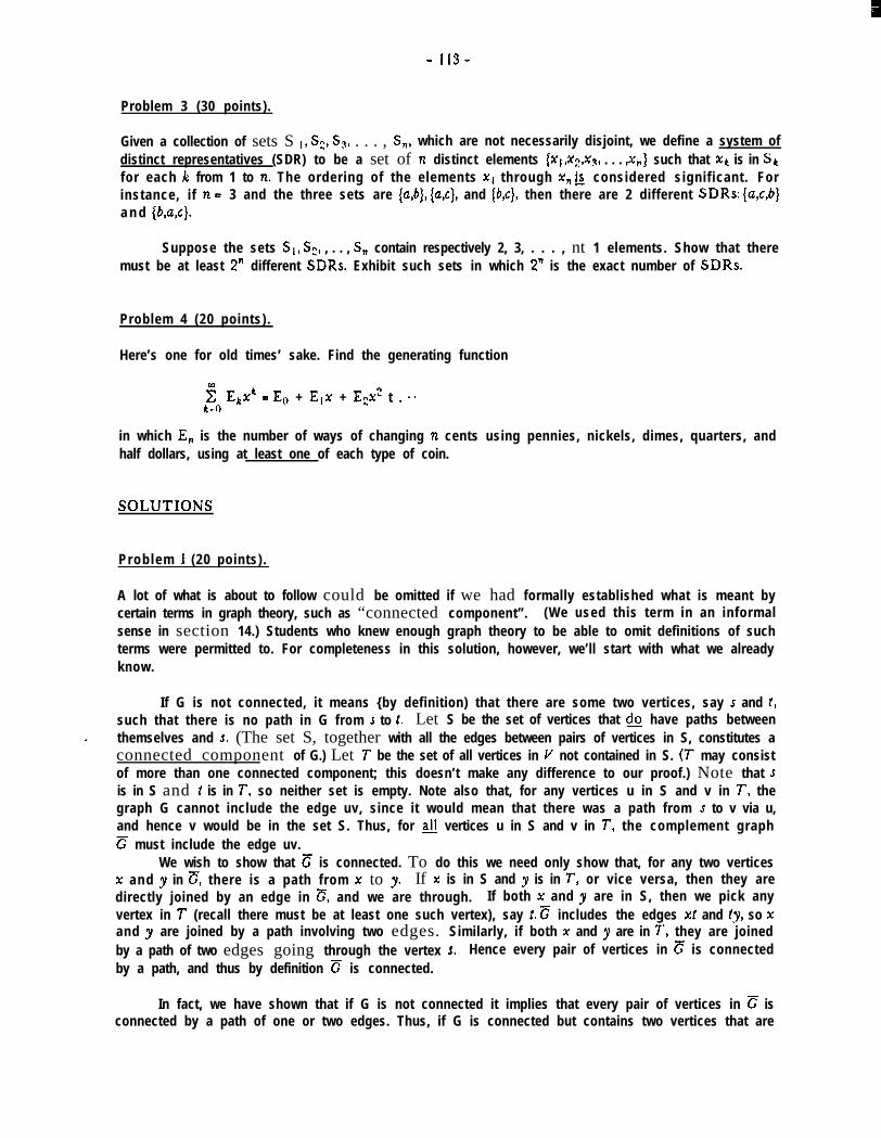
- 113-

Problem 3 (30 points).

Given a collection of sets S ,, S:, S3, . . . , S,, which are not necessarily disjoint, we define a system ofdistinct representatives (SDR) to be a set of n distinct elements {xi,xz,x9, . . . J,) such that xk is in SI:for each It from 1 to n. The ordering of the elements xl through x, k considered significant. Forinstance, if n - 3 and the three sets are {a,bj, (a,c), and {b,c), then there are 2 different SDRs: (a,~&a n d (b,a,c).

Suppose the sets Si, S=, , . . , S, contain respectively 2, 3, . . . , nt 1 elements. Show that theremust be at least 2” different SDRs. Exhibit such sets in which 2” is the exact number of SDRs.

Problem 4 (20 points).

Here’s one for old times’ sake. Find the generating function

$ Ehx’kr0

= Et, + E,x + E$ t . a n

in which E, is the number of ways of changing n cents using pennies, nickels, dimes, quarters, andhalf dollars, using at least one of each type of coin.

SOLUTIONS

Problem 1 (20 points).

A lot of what is about to follow could be omitted if we had formally established what is meant bycertain terms in graph theory, such as “connected component”. (We used this term in an informalsense in section 14.) Students who knew enough graph theory to be able to omit definitions of suchterms were permitted to. For completeness in this solution, however, we’ll start with what we alreadyknow.

If G is not connected, it means {by definition) that there are some two vertices, say 5 and t,such that there is no path in G from J to 2. Let S be the set of vertices that do have paths between

a themselves and J. (The set S, together with all the edges between pairs of vertices in S, constitutes aconnected component of G.) Let T be the set of all vertices in V not contained in S. (T may consistof more than one connected component; this doesn’t make any difference to our proof.) Note that 5is in S and i is in T, so neither set is empty. Note also that, for any vertices u in S and v in T, thegraph G cannot include the edge uv, since it would mean that there was a path from s to v via u,and hence v would be in the set S. Thus, for fi vertices u in S and v in T, the complement graphc must include the edge uv.

We wish to show that c is connected. To do this we need only show that, for any two verticesx and y in c, there is a path from x to y. If x is in S and y is in T, or vice versa, then they aredirectly joined by an edge in c, and we are through. If both x and y are in S, then we pick anyvertex in T (recall there must be at least one such vertex), say t. c includes the edges xr and ry, so SCand y are joined by a path involving two edges. Similarly, if both x and y are in T, they are joinedby a path of two edges going through the vertex s. Hence every pair of vertices in c is connectedby a path, and thus by definition c is connected.

In fact, we have shown that if G is not connected it implies that every pair of vertices in c isconnected by a path of one or two edges. Thus, if G is connected but contains two vertices that are

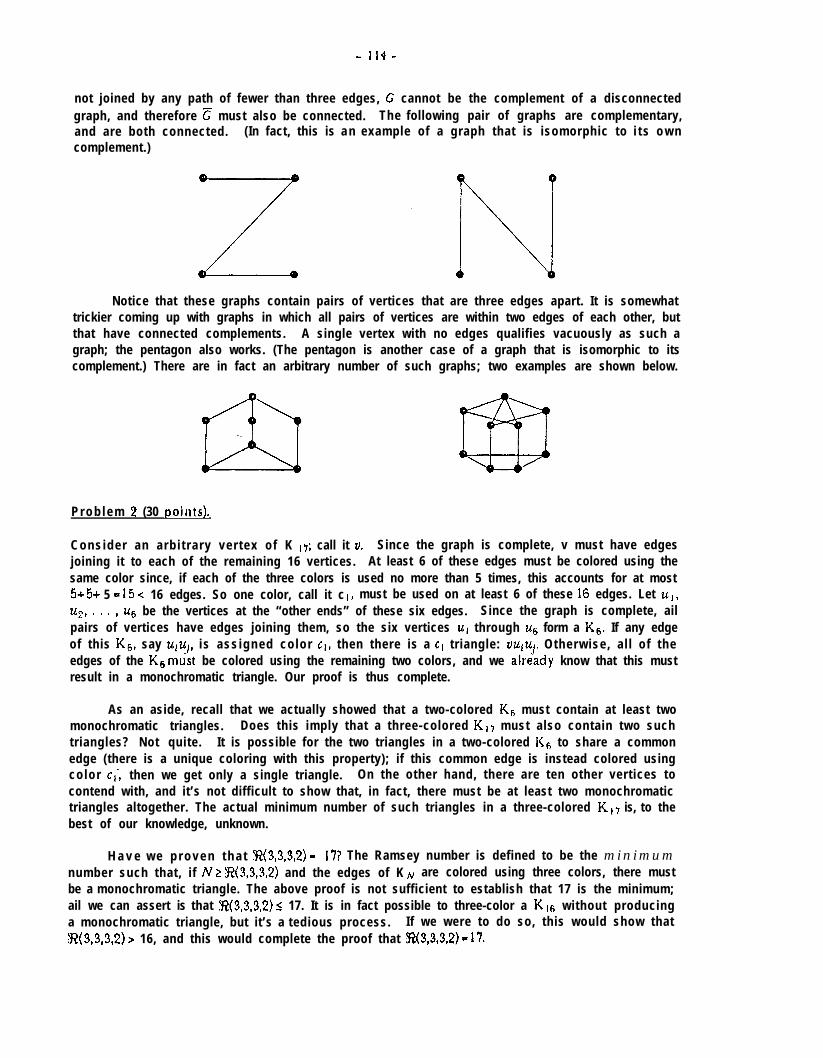
- 114-

not joined by any path of fewer than three edges, G cannot be the complement of a disconnectedgraph, and therefore c must also be connected. The following pair of graphs are complementary,and are both connected. (In fact, this is a n example of a graph that is isomorphic to i t s o w ncomplement.)

Notice that these graphs contain pairs of vertices that are three edges apart. It is somewhattrickier coming up with graphs in which all pairs of vertices are within two edges of each other, butthat have connected complements. A single vertex with no edges qualifies vacuously as such agraph; the pentagon also works. (The pentagon is another case of a graph that is isomorphic to itscomplement.) There are in fact an arbitrary number of such graphs; two examples are shown below.

P r o b l e m 2 (30 poillts).

Consider an arb i t rary ver tex of K ,f; call it v. Since the graph is complete, v must have edgesjoining it to each of the remaining 16 vertices. At least 6 of these edges must be colored using thesame color since, if each of the three colors is used no more than 5 times, this accounts for at most5+5+ 5 = 15 < 16 edges. So one color, call it c I, must be used on at least 6 of these 16 edges. Let uI,u2, * ’ ’ I u6 be the vertices at the “other ends” of these six edges. Since the graph is complete, ailpairs of vertices have edges joining them, so the six vertices uI through u-6 form a Kg. If any edgeof this K6, say ufuI, is ass igned co lor cl, then there is a cl triangle: vuiuI. Otherwise, a l l of theedges of the K6 m&t be colored using the remaining two colors, and we aire‘ady know that this mustresult in a monochromatic triangle. Our proof is thus complete.

As an aside, recall that we actually showed that a two-colored Kfi must contain at least twomonochromatic triangles. Does this imply that a three-colored K,t must also contain two suchtriangles? Not quite. It is possible for the two triangles in a two-colored Kh to share a commonedge (there is a unique coloring with this property); if this common edge is instead colored usingcolor c,‘, then we get only a single triangle. On the other hand, there are ten other vertices tocontend with, and it’s not difficult to show that, in fact, there must be at least two monochromatictriangles altogether. The actual minimum number of such triangles in a three-colored KI, is, to thebest of our knowledge, unknown.

H a v e w e p r o v e n t h a t 9?(3,3,3,2) = 171 The Ramsey number is defined to be the m i n i m u mnumber such that, if /V 2 Y?(3,3,3,2) and the edges of K ,,, are colored using three colors, there mustbe a monochromatic triangle. The above proof is not sufficient to establish that 17 is the minimum;ail we can assert is that R(3,3,3,2) ,( 17. It is in fact possible to three-color a K16 without producinga monochromatic triangle, but it’s a tedious process. If we were to do so, this would show that%(3,3,3,2) > 16, and this would complete the proof that R(3,3,3,2) - 17.

- 115-

Problem 3 (30 points).

Some people approached this problem by first asserting something to the effect of, “The minimumnumber of distinct SDRs is achieved when there is maximum containment among the sets, i.e., whens, cs~c&c.**cs,.” These people then proceeded to show that, in this situation, there areexactly 2” SDRs, and claimed that therefore there are always at least that many. This is going aboutit backwards. How do we know that the minimum occurs when there is maximum containment? Itmay be intuitively obvious, but that’s not a pro& In fact, the most reasonable way to prove it is toshow that maximum containment results in 2” SDRs and that there are always at least 2” SDRs, andconclude that the minimum occurs when there is maximum containment. Just to claim that theminimum occurs with maximum containment, and use this claim to conclude that there are always atleast 2” SDRs, is circular logic. So let’s prove this the right way!

If n = 1, then S, consists of two elements, xl and x2, and there are obviously 2’ = 2 possibleSDRs, namely (x,) and (x,>. So the result is true for n = 1. We’ll use induction to prove it is truefor any finite n .

Suppose the result is true for n-l. That is, given n-l sets containing respectively 2, 3, . . . , nelements, there are at least 2”-’ different SDRs. Now consider the situation when another set, withn+ 1 elements, is added to the collection. We know, by the induction hypothesis, that there are atleast 2”-’ ways to cbloose n-l distinct elements, one from each of the first n-l sets (where the order ofselection is considered to be significant). For each such choice, there are at least two choices for theelement to represent the last set. Why? The set contains n+l elements, and at most n-i of them canbe included among the elements already in the SDR. Therefore there are at least 2 elements thathave not yet been chosen and are therefore eligible to represent this set. Since there are at least 2R-’ways to choose the first n-l elements and, for each choice, at least 2 ways to choose the last element,there are at least 202”~’ = 2” ways to choose the n elements of the SDR.

Ifs, c scl c s, c***c s,, then there are again exactly 2 SDRs for the single set S,. Thistime, however, khen ‘we add the 71th set to the collection, there are, for each possible SDR for thefirst n-l sets, exactly two choices for the element that will represent S,. This is because, no matterwhich elements are chosen to represent the first n-l sets, these n-l elements must be contained in S,,and thus exact ly n-l of the ntl elements in Sn are ineligible to represent it, leaving exactly twochoices. Thus, by induction, there are exactly 2” SDRs for these sets. One specific example of sucha case is the collection of sets (a,b), (a&), {a&&). There are exactly eight distinct SDRs for thesesets, n a m e l y (a,b,c), (a,W}, {a,c,b), {a,c,dJ, (b,w), {had}, (ka}, and {k@a

Problem 4 (20 points).

-The only real difficulty with this problem seemed to be some confusion over exactly what constitutes-a “generating function”. The summation

: Ekxkk - 0

= Er, t E,x t E=x2 + a m m

is a generating function for the sequence Eo, El, EZ, etc., but is not very useful in this form. Forinstance, in section 3 of the notes, we found a generating function that could be written in the aboveform, where En was the number of ways of changing n cents using five types of coins (without therestriction that each type be used at least once). However, writing the function as a summation likethis is not useful, since it does not help us find the coefficients En. On the other hand, the set ofrecursion formulas that we proceeded to find for computing En were not themselves a generatingfunction; they were simply a means for computing the coefficients of the generating function. The

- 116-

function itself w a s

(I-x)( I-x5)( I-x’“)( j+F5)( I-P) *

The whole idea of using a generating function is that we want to be able to deal with the infinitesequence as a s’ngie unit; we want a finite form that “embodies” the infinite sequence. The infinitesummation tells us what the generating function “IS” ‘n the sense that it tells us what it represents.The finite formula shown above tells us what the generating function “is” in the sense that it givesus a mathematical means for expressrng it. Since the infinite summation is trivial to specify (and i nfact was given as part of the statement of the problem), it is obviously the finite formula that iscalled for.

There are two “easy” ways to f’nd the desired function- using either the method or the resultfrom section 3 of the notes. Using the result is easier, so let’s do it that way first. We observe thatone way to provide change for n cents, using at least one of each type of coin, is to start by settingaside the five required coins, after which we may use any combination of coins for the remainingamount. T h e five required coins have a value of 1+5+10+25+50 = 91 cents. Thus, to change ncents, we set aside 91 cents and then change n-91 cents using any coins we wish. Let E’, representthe number of ways of changing n cents, without the restriction that at least one of each type of coin.be used. W e know f rom sect’on 3 that

i! E’kX’ = - 1k - 0 ( 1 -x)( 1 -x5)( I-x I”)( 1 gJ)( j-p) *

Meanwhi le , we have just shown that En = E’+gl. Hence

= fii E’kq,,Xkk-0’

(since we know E’, = 0 for ail n < 0). W e then let j - k-91 on the righthand side and f i n d

g Ekxk = ; E’pl*c”k4 .1-C’

which is the desired result.

Meanwhile, we could also have started from scratch and used the method described in section3. We would find that we could use one penny, or two, or three, etc., but not zero, and would writethese choices as the in f in i te sum, x t x2 t xJ t l 9 B .t h r e e , e t c . , g i v i n g t h e s u m x5 t x’(’ t xl5 t e l 9 .

Similarly, we could have one nickel, or two, orContinuing in this fashion, we would eventually

take the product of these sums, thus:

(x+3c2+xSt * * - )(x5++x'o+x'5+ - * * )(x'"+x20tpt * ' ' )(x25tx50+x'5t ' ' * )(xwtx'Dotx'w+ ' * ' ) .

- 117-

Each term of the product with an exponent of n corresponds to one way of selecting a term fromeach sum such that the exponents sum to n. Now, since

(and similarly for the other sums), we would find that the desired generating function is

x x5 x II) $5 $8-.-.

jg l j-g jmx10 1_x’5 l i-p 9

which is equivalent to our earlier answer.

Q, Aiexandru T. Baiaban (editor), Chemical Applications of Graph Theory.

0 Claude Berge, Principes de Combinatoire,

e Lester Ford, Jr.,.and Deibert Fuikerson, Florus in Netruorks.

Q Marshall Hail, Jr., Combinatorial Theory.

0 Frank Harary, Graph Theory .

@ Frank Harary (editor), A Seminar on Graph Theory.

@ Donald E. Knuth, The Art of Computer Programming.

Q C. L. Liu, introduction to Combinatorial Mathematics.

o E. Netto, Lehrbuch de Combinatorik (2nd edition, 1927).

Q George Pbiya, Hozu to Solve It. [HSI]

Qp George P6iya, Mathematical Discovery. [MD]

0 George P6iya, Mathematics and Plausible Reasoning. EMPRI

0 George P6iya and Gabor Szegij, Problems and Theorems in Analysis. EP-SzJ

0 John Riordan, An Introduction to Combinatorial Analysis.

0 Herbert J. Ryser, Combinatorial Mathematics.

0 Thomas L. Saaty and Paul C. Kainen, The Four-Color Problem.

I

1

I

I

I

I

,’

,’