notes for course ee1.1 circuit analysis 2004-05 topic 8

Notes for course EE1.1 Circuit Analysis 2004-05

TOPIC 8 – DEPENDENT SOURCES

Objectives

To introduce dependent sources

To study active sub-circuits containing dependent sources

To perform nodal analysis of circuits with dependent sources

1 INTRODUCTION TO DEPENDENT SOURCES

1.1 General

The elements we have introduced so far are the resistor, the capacitor, the inductor, the independentvoltage source and the independent current source.

These are all 2-terminal elements

The power absorbed by a resistor is non-negative at all times, that is it is always positive or zero

The inductor and capacitor can absorb power or deliver power at different time instants, but theaverage power over a period of an AC steady state signal must be zero; these elements are calledlossless.

Since the resistor, inductor and capacitor cannot deliver net power, they are passive elements.

The independent voltage source and current source can deliver power into a suitable load, such as aresistor.

The independent voltage and current source are active elements.

In many situations, we separate the sources from the circuit and refer to them as excitations to thecircuit.

If we do this, our circuit elements are all passive.

In this topic, we introduce four new elements which we describe as dependent (or controlled)sources.

Like independent sources, dependent sources are either voltage sources or current sources.

However, unlike independent sources, they receive a stimulus from somewhere else in the circuitand that stimulus may also be a voltage or a current, leading to four versions of the element

Dependent sources are considered part of the circuit rather than the excitation and have the functionof providing circuit elements which are active; they can be used to model transistors and operationalamplifiers.

Since there are two source terminals and also two terminals where the stimulus exists, dependentsources are in general 4-terminal elements.

1.2 An Intuitive Analogy for Dependent Sources

The basic idea of the voltage-controlled voltage source can be illustrated by considering a voltagesource vc connected between two nodes and a voltmeter connected between two different nodesbetween which there exists a voltage difference vx:

Topic 8 – Dependent Sources

2

The voltmeter measures the voltage vx and then controls the voltage source such that vc = µvx.

Since the electrical equivalent of an ideal voltmeter is an open circuit, we can represent the elementas follows:

The basic idea of the current-controlled current source can be illustrated by considering a currentsource ic connected between two nodes and an ammeter connected between two different nodesbetween which a current ix flows:

The ammeter measures the current ix and then controls the current source such that ic = βix.

Since the electrical equivalent of an ideal ammeter is a short circuit, we can represent the element asfollows:

In these examples, the output variable vc or ic is called the controlled variable and the input variablevx or ix is called the controlling variable.

The remaining two source types are obtained by combining controlled and controlling variables indifferent ways.

For instance, the voltage-controlled current source combines open-circuit voltage measurement witha current source at the output; it is described by ic = gmvx:

The current-controlled voltage source combines short-circuit current measurement with a voltagesource at the output; it is described by vc = rmix:

Thus the four types of dependent sources are as follows:


3

VCVS VCCS CCVS CCCS

Dependent (or controlled) sources can be thought of intuitively as amplifiers, where the input andoutput variables can both be either a voltage or a current.

In many cases, there is some flexibility over which type of source can be used.

For example, when the load is resistive, it may be driven by a voltage source or a current sourcebecause the voltage and current are related by Ohm's law.

1.3 The Dependent Voltage Source

Although dependent sources are strictly 4-terminal elements, we can show them simply as a voltageor current source and write next to it an expression for the voltage or current as a function ofanother voltage or current defined elsewhere in the circuit.

Using this notation, the symbol for a dependent voltage source is as follows:

where vx and ix are defined elsewhere in the circuit.

Its outline is a diamond shape to show that it is a dependent source and to distinguish it from theround-shaped independent voltage source.

Inside the diamond shape, a pair of '+' and '–' signs denote the positive reference for the voltagegenerated.

The terminal voltage v of the dependent voltage source, when plotted as a function of its terminalcurrent i, is exactly the same as that of an independent voltage source:

This plot shows that vc is independent of i. However, whereas for an independent voltage source,the voltage is also constant with time, in the case of the dependent voltage source, the voltagedepends upon either a voltage vx or a current ix somewhere else in the circuit and is therefore not, ingeneral, constant with time.

Voltage vc is referred to as the controlled voltage (or dependent voltage).

When the controlling variable is a voltage, the dependent voltage source is called a voltage-controlled voltage source, or VCVS; the dependency relationship has the form:

vc = µvxThe parameter µ is a unit-less real constant called the voltage gain.

When the controlling variable is a current, the dependent voltage source is called a current-controlled voltage source (or CCVS); the linear dependency relationship takes the form


4

vc = rmixThe real constant rm has units of Ohms and is called the trans-resistance.

The prefix "trans" is used because the dependent source "transfers" the effect of a currentsomewhere else in the circuit to the dependent voltage source; the term "resistance" is used becauseit multiplies that current by a constant having the unit of Ω to turn it into a voltage.

The subscript "m" denotes "mutual" which is a synonym for "trans".

The CCVS, however, is quite different from the resistor element because the current in a resistorelement must be defined in the same element as that across which the voltage is defined.

We could say that a resistor has self-resistance (or just resistance) and that a CCVS has mutualresistance or trans-resistance.

1.4 The Dependent Current Source

The symbol for a dependent current source is as follows:

It has the same diamond shape as that of the dependent voltage source, but instead of '+' and '–'signs, it has an arrow denoting the positive current reference for the controlled current ic.

The v-i characteristic has the following form:

It has the same terminal behaviour as that of an independent current source, but the value of thecontrolled current ic depends upon either a voltage vx or a current ix somewhere else in the circuitand will therefore in general vary with time.

When the controlling variable is a voltage, we refer to the dependent i-source as a VCCS, forvoltage-controlled current source; the dependency relationship is:

ic = gmvxThe real constant gm has units of Siemens and is therefore called the trans-conductance.

When the controlling variable is a current,, we refer to the dependent i-source as a CCCS, forcurrent-controlled current source; the dependency relationship is:

ic = βixThe real unit-less constant β is called the current gain.

We develop a method for analysing a circuit containing dependent sources by considering someexamples.

1.5 Dependent Source Examples

Example 5.1: Find the value of current i in the circuit shown which contains a CCCS:


5

Solution

Note that the current-controlled current source is defined by ic = 2ix, where ix is the current in the 6Ω resistor.

Note that for a dependent source, the polarities for the controlling variable and controlled variableare inter-related and neither should be changed separately.

We treat the dependent source constraint relationship ic = 2ix as a label on the source.

We temporarily cover this label with a small piece of tape on which we write the symbol ic; we callthis procedure taping the dependent source.

This leads to the following:

We now treat ic as if it was an independent current source, just like the 9 A current source.

The current divider rule leads to:

i = − 9 + ic( ) 63+ 6

= −6 − 23ic

If ic was an independent current source, we would be through; however, for a dependent sourcethere is a further stage:

We next un-tape the dependent source and express its controlled variable ic in terms of itscontrolling variable:

ic = 2ixWe then express the controlling variable in terms of our analysis variables, in this case the unknowncurrent i.

Using KCL, we have:

ic = 2ix = 2 9 + i + ic( )Note that ic appears on both sides of the equation. We can now solve the two equations:

ic = 2 9 + i + ic( ) = 18 + 2i + 2icic = −18 − 2i

i = −6 −23ic = −6 +

23

18 + 2i( ) = 6 +43i

i = −−61 3

= −18 A

We can state the general method of analysis as follows:

1) Tape all dependent sources, thus treating them temporarily as independent sources.


6

2) Analyze the circuit for the unknown variable or variables you have chosen using theanalysis technique of your choice.

3) Un-tape the dependent sources and express their values in terms of the unknowns you havechosen to use in step 2.

4) Solve the resulting equations.

Example 5.2: Find the voltage v in the following circuit which contains a CCVS:

Solution

We show the circuit also with the dependent source taped.

We can use voltage division to compute v:

v = 44 + 6

vc − 24( ) = 25vc −

485

If vc were a known quantity, we would be through.

As it is not, we un-tape the dependent source and express its value in terms of the unknown voltagev:

vc = 2ix = 2 24 − vc10

⎛⎝⎜

⎞⎠⎟=

245

−vc5

6vc = 24 vc = 4 V

Then we use the previous equation to obtain v:

v = 25× 4 −

485

= −8 V

2 ACTIVE SUB-CIRCUITS

2.1 General

In this section, we use hand analysis techniques to look at unusual behaviour of circuits containingdependent sources and at their Thevenin and Norton equivalents.

In the following section we will cover the extension of the systematic nodal analysis method toinclude dependent sources.

2.2 Unusual behaviour of sub-circuits containing dependent sources

Active subcircuits may be defined as any subcircuit containing one or more dependent sources.

Circuits consisting of passive elements and independent voltage and current sources always have asolution, provided we avoid some obviously problematical situations, such as a loop of voltagesources or a cut-set of current sources.

An example of a loop of voltages sources is as follows:


7

Circuit De-activated circuit

A cut-set of current sources describes the situation where de-activating current sources divides thecircuit into two separate parts:

Circuit De-activated circuit

If we avoid these situations, any circuit with any element values is soluble.

In the case of active circuits containing dependent sources, this is not the case and it is very easy togenerate circuits which do not have any solution; in practice, they are unstable; there is no uniqueset of finite nodal voltages and branch currents which satisfies Kirchhoff's laws.

We now give some examples of such behaviour.

Consider the simple subcircuit shown:

The circuit consists of a CCVS whose controlling variable ix is equal to the terminal current i.

Analysis of the circuit to find its v–i relationship gives:

v = −2ivi= −2

where we have used the normal polarity conventions for v and i.

We see that this subcircuit is equivalent to a resistor; however, the resistance value is negative.

The power absorbed by the subcircuit is:

P = v × i = −2i( ) × i = −2i2

which is negative if the current is nonzero.

Hence, the energy (the time integral of power) is also negative and the negative resistor can deliverenergy to the external circuit; the subcircuit is clearly an active one.

Consider a slightly more complicated subcircuit:


8

We have just added an ordinary resistor element in series with the same CCVS with trans-resistancerm.

We know from our preceding discussion that the CCVS is equivalent to a negative resistor whosevalue is –rm.

Thus the equivalent subcircuit is as shown above.

Now, if rm is set equal to R, then the equivalent resistance is zero! This means that the subcircuit isequivalent to a short circuit.

So, if this sub-circuit was connected across a voltage source, there would be a conflict of voltagesand the circuit would not be soluble, even though this is not obvious from the circuit topology.

2.3 Thevenin and Norton equivalents for circuits containing dependent sources

We explore this topic by considering an example.

Example 5.4: For the 2-terminal subcircuit shown:

a. Find the Thevenin and Norton equivalents for general values of β.

b. Evaluate the parameters of these equivalents for β = 1 and β = 2.

Solution

Note that this circuit contains a CCCS controlled by the current in the 2 Ω resistor.

We start by taping the dependent source:

We have attached an independent current source to the terminals as a test source.


9

We have drawn an imaginary closed surface around the dependent source and its parallel resistor tohelp understand the derivation of the following KCL equation:

ix = is + i

Furthermore, KCL applied to the node at the junction of the applied test source and the dependentsource gives a current of i – ic through the resistor inside the surface.

Thus, by KVL around the loop consisting of the two resistors and the applied test source, we have

v = 2 i + is( ) + 2 i − ic( )We next un-tape the dependent source:

ic = βix = β i + is( )Using this in the other equation gives:

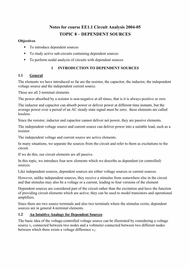
v = 2 i + is( ) + 2 i − ic( ) = 2 i + is( ) + 2i − 2β i + is( ) = 2 1− β( )is + 2 2 − β( )iSince v has a constant part and a part proportional to i, we can now identify the Theveninparameters, leading to the Thevenin equivalent circuit:

The Norton equivalent obtained by rearranging the equation for v in terms of i:

i = −1− β2 − β

is +1

2 2 − β( ) v

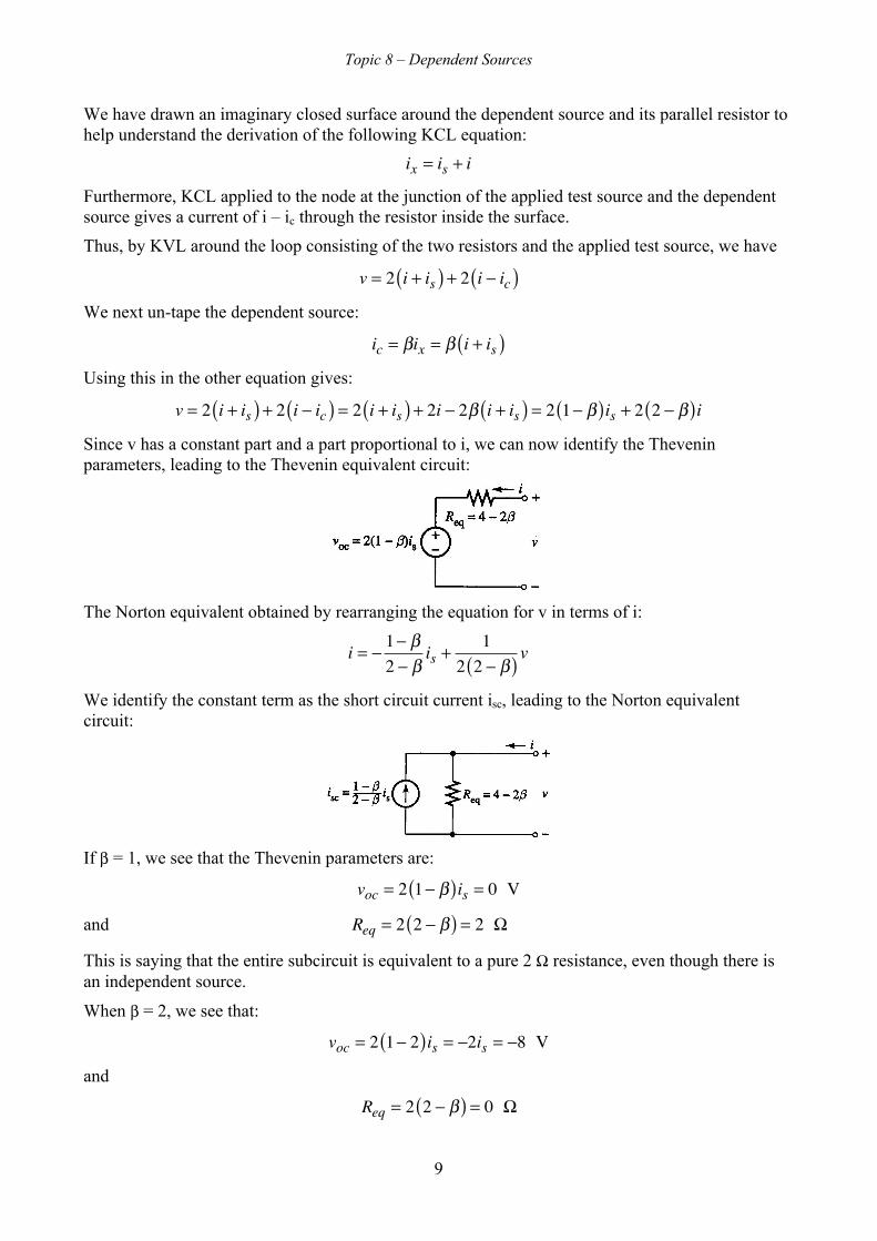
We identify the constant term as the short circuit current isc, leading to the Norton equivalentcircuit:

If β = 1, we see that the Thevenin parameters are:

voc = 2 1− β( )is = 0 V

and Req = 2 2 − β( ) = 2 Ω

This is saying that the entire subcircuit is equivalent to a pure 2 Ω resistance, even though there isan independent source.

When β = 2, we see that:

voc = 2 1− 2( )is = −2is = −8 V

and

Req = 2 2 − β( ) = 0 Ω


10

Thus, we have two completely different Thevenin equivalent circuits for different β values:

β = 1 β = 2

Example 5.6: Consider the circuit shown:

a) If β = 0.5, find the value of R that results in maximum power absorbed by R.

b) If β = 1.5, find the value of R that results in maximum power absorbed by R.

Solution

The first step is to tape the dependent source; we also attach a test source in the place of the resistorR:

We have shown the resistor currents obtained by applying KCL to the top and middle nodes.

KVL now implies that:

v = 4 i + is( ) + 4 i + is + ic( ) = 8is + 4ic + 8iUn-taping the dependent source, we obtain:

ic = 0.5ix = 0.5 i + is + ic( )Solving this last equation for ic and using the resulting value in the previous equation gives:

v = 24 +12iThus, we know that Req = 12 Ω and we must therefore make R = 12 Ω for maximum power transfer.

If we let β = 1.5 when we un-tape, the resulting equation (5.2-37) becomes

ic = 1.5ix = 1.5 i + is + ic( )Solving for ic and using the resulting value above now gives:

v = −8 − 4iThe equivalent resistance is now negative and the original derivation of the maximum powertransfer condition, which assumed positive resistor values, is no longer valid.


11

For example, if we make R = 4 Ω, then an infinite current will flow and the power transferred willbe infinite!

3 NODAL ANALYSIS OF CIRCUITS WITH DEPENDENT SOURCES

We have stated that dependent sources have exactly the same v-i characteristics as theirindependent cousins; the only difference is that there is an added algebraic constraint requiring thattheir values be proportional to some other voltage or current in the circuit.

We will now use this observation to extend our techniques of nodal and mesh analysis to activecircuits with the following step-by-step algorithm.

1) Tape all the dependent sources, thus temporarily treating them as independent sources.

2) Perform nodal analysis in order to determine the nodal equations or write them byinspection.

3) Un-tape the dependent sources and express the value of each in terms of the node voltages.

4) Solve the resulting modified nodal equations for the node voltages.

The procedure for nodal analysis for circuits with dependent sources are similar to those for circuitswithout them.

Therefore we will illustrating the method by means of examples.

In these examples, the dependent source parameter values are such that a unique solution exists.

Example 5.7: Find the value of i in the circuit in the following circuit using nodal analysis:

Solution

Our first step is to tape the single dependent source and to prepare the circuit for nodal analysis byassigning a reference node and labelling the non-reference nodes with node voltage symbols:

KCL can be applied at the two labelled essential nodes.

Alternatively, the inspection method yields the matrix form of the nodal equations:

14+16

−16

−16

18+16

⎡

⎣

⎢⎢⎢⎢

⎤

⎦

⎥⎥⎥⎥

v1v2⎡

⎣⎢

⎤

⎦⎥ =

15 − icic

⎡

⎣⎢

⎤

⎦⎥


12

Next, we un-tape the dependent source and express its value in terms of the unknown node voltagesv1 and v2:

ic = 2ia = 2v14=v12

Inserting this in the nodal equation gives:

14+16

−16

−16

18+16

⎡

⎣

⎢⎢⎢⎢

⎤

⎦

⎥⎥⎥⎥

v1v2⎡

⎣⎢

⎤

⎦⎥ =

15 − v12

v12

⎡

⎣

⎢⎢⎢⎢

⎤

⎦

⎥⎥⎥⎥

The v1 terms on the RHS of the equation really belong on the LHS and they can be simplytransferred across:

14+16+12

−16

−16−12

18+16

⎡

⎣

⎢⎢⎢⎢

⎤

⎦

⎥⎥⎥⎥

v1v2⎡

⎣⎢

⎤

⎦⎥ =

150

⎡

⎣⎢

⎤

⎦⎥

Notice that it is only the elements in the first column that are multiplied by v1 that are modified bythis transfer. Note that the terms proportional to v1 on the RHS disappear leaving only constants.

The solution is: v1 = 28 V, v2 = 64 V

Referring to the circuit diagram, we have: i = –v2/8 = –8 A

Example 5.9: Find the value of v in the following circuit using nodal analysis.

Solution

The circuit prepared for nodal analysis is as follows:

Both dependent sources have been taped.

We have identified a supernode (shown shaded) and an essential node (also shaded).

The matrix equations may be written using the by-inspection method:


13

14+12+12

−12

−12

14+12

⎡

⎣

⎢⎢⎢⎢

⎤

⎦

⎥⎥⎥⎥

v1v2⎡

⎣⎢

⎤

⎦⎥ =

−5 − ic −162−vc2

5 + vc2

⎡

⎣

⎢⎢⎢⎢

⎤

⎦

⎥⎥⎥⎥

Un-taping the CCVS, we have:

vc = 8ix = −8 v1 +162

= −4v1 − 64

Un-taping the VCCS, we have:

ic =34vy =

34v2 − v1 + vc( )⎡⎣ ⎤⎦ =

34v2 +

94v1 + 48

The un-taped nodal equations are now:

14+12+12

−12

−12

14+12

⎡

⎣

⎢⎢⎢⎢

⎤

⎦

⎥⎥⎥⎥

v1v2⎡

⎣⎢

⎤

⎦⎥ =

−29 − 14v1 −

34v2

−27 − 2v1

⎡

⎣

⎢⎢

⎤

⎦

⎥⎥

Moving the terms involving the node voltages on the RHS to the LHS yields:

14+12+12+14

−12+34

−12+ 2 1

4+12

⎡

⎣

⎢⎢⎢⎢

⎤

⎦

⎥⎥⎥⎥

v1v2⎡

⎣⎢

⎤

⎦⎥ =

−29−27⎡

⎣⎢

⎤

⎦⎥

This may be tidied up:

32

14

32

34

⎡

⎣

⎢⎢⎢⎢

⎤

⎦

⎥⎥⎥⎥

v1v2⎡

⎣⎢

⎤

⎦⎥ =

−29−27⎡

⎣⎢

⎤

⎦⎥

The solution is v1 = –20 V and v2 = 4 V. Hence, v = v2 = 4 V.

For a passive circuit, we noticed that the nodal conductance matrix was always symmetrical.

We can see form the examples in this section that the effect of introducing dependent sources into acircuit is to change the admittance matrix from a symmetrical one to an unsymmetrical one.

If a conductance matrix is unsymmetrical, then it must be the conductance matrix for an activecircuit containing dependent sources.

4 CONCLUSIONS

We have introduced the dependent sources as a new type of element that has 4 terminals and isactive, ie it can deliver power to other elements.

We have studied active sub-circuits containing dependent sources and shown that they can realisenegative resistance and that circuits using dependent sources may not always be soluble.

Finally, we found that the systematic by-inspection method of nodal analysis can be extended in astraightforward way to analyse circuits with dependent sources

notes for course ee1.1 circuit analysis 2004-05 topic 8

Documents