normalized cuts and image segmentation amir lev-tov idc, herzliya advanced topics in computer vision
TRANSCRIPT

Normalized Cuts and Normalized Cuts and Image SegmentationImage Segmentation
Amir Lev-TovAmir Lev-TovIDC, HerzliyaIDC, Herzliya
Advanced Topics in Computer Vision
[1] Normalized Cuts and Image [1] Normalized Cuts and Image Segmentation, Shi and Malik, IEEE Conf. Segmentation, Shi and Malik, IEEE Conf. Computer Vision and Pattern Recognition, Computer Vision and Pattern Recognition, 1997.1997.
[2] Normalized Cuts and Image [2] Normalized Cuts and Image Segmentation, Shi and Malik, IEEE Segmentation, Shi and Malik, IEEE Transactions on pattern analysis and Transactions on pattern analysis and machine intelligence, Vol 22, No 8, 2000machine intelligence, Vol 22, No 8, 2000
Main ReferencesMain References

More ReferencesMore References
[3] Weiss Y[3] Weiss Y. . Segmentation using eigenvectorsSegmentation using eigenvectors: : a a unifying viewunifying view.. Proceedings IEEE International Proceedings IEEE International Conference on Computer Vision, 1999.Conference on Computer Vision, 1999.
[4] Ng A.Y., Jordan , M.I., and Weiss Y, On [4] Ng A.Y., Jordan , M.I., and Weiss Y, On Spectral Clustering: Analysis and an algorithm, Spectral Clustering: Analysis and an algorithm, NIPS 2001 NIPS 2001
[5] Rayleigh’s Quotient, Nail Gumerov, 2003[5] Rayleigh’s Quotient, Nail Gumerov, 2003 [6] Wu and Leahy, an optimal graph theoretic [6] Wu and Leahy, an optimal graph theoretic
approach to data clustering, PAMI, 1993approach to data clustering, PAMI, 1993

Mathematical IntroductionMathematical Introduction
Definition: is an Definition: is an Eigen Value Eigen Value of n x n of n x n matrix A, if there exist a non-trivial vector matrix A, if there exist a non-trivial vector
such that: such that: That vector is called That vector is called Eigen VectorEigen Vector of A of A
corresponding to the Eigen Value corresponding to the Eigen Value All Eigenvectors correspond to different All Eigenvectors correspond to different
Eigenvalues, are mutually linearlly Eigenvalues, are mutually linearlly independent (Orthogonal set).independent (Orthogonal set).
0v Av v
v

Mathematical IntroductionMathematical Introduction
Matrix A is called Matrix A is called HermitianHermitian if if Where A* is the Where A* is the conjugate transpose conjugate transpose of A:of A:
Real matrix is Hermitian Real matrix is Hermitian Symmetric Symmetric Let A be a Hermitian matrix.Let A be a Hermitian matrix.
Then Then
is called the is called the Rayleigh’s QuotientRayleigh’s Quotient of A. of A.
* tA A
*A A
*
*( , )
v AvR A v
v v

Mathematical IntroductionMathematical Introduction
For real matrices the definition becomes:For real matrices the definition becomes:
Where A is just symmetric.Where A is just symmetric.
( , )t
t
v AvR A v
v v

Mathematical IntroductionMathematical Introduction
TheoremTheorem: Rayleigh’s Quotient gets its : Rayleigh’s Quotient gets its minimum value at A’s minimal eigenvalue,minimum value at A’s minimal eigenvalue,
and the corresponding eigenvector and the corresponding eigenvector
achieve this minimum.achieve this minimum. Moreover: if A has n eigenvalues Moreover: if A has n eigenvalues
then R(A,v) has n stationary points then R(A,v) has n stationary points achieved at their eigenvectorsachieved at their eigenvectors respectively.respectively.
11v
1{ ,..., }n
1{ ,..., }nv v
Mathematical IntroductionMathematical Introduction
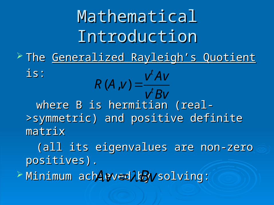
The The Generalized Rayleigh’s QuotientGeneralized Rayleigh’s Quotient
is:is:
where B is hermitian (real->symmetric) where B is hermitian (real->symmetric) and positive definite matrixand positive definite matrix
(all its eigenvalues are non-zero positives).(all its eigenvalues are non-zero positives). Minimum achieved by solvingMinimum achieved by solving::
( , )t
t
v AvR A v
v Bv
Av Bv

Segmentation IntroductionSegmentation Introduction

Segmentation IntroductionSegmentation Introduction
Problem: Divide an image into subsets of Problem: Divide an image into subsets of pixels (Segments).pixels (Segments).
Some methods: Some methods: ThresholdingThresholding Region GrowingRegion Growing KK--meansmeans MeanMean--ShiftShift Use of changes in color, texture etc.Use of changes in color, texture etc. ContoursContours

Segmentation IntroductionSegmentation Introduction
The problem is not very well defined, for The problem is not very well defined, for example, how many groups are in the example, how many groups are in the picture? 4? Maybe 3 ? 2? Or even every Xpicture? 4? Maybe 3 ? 2? Or even every X
Segmentation IntroductionSegmentation Introduction
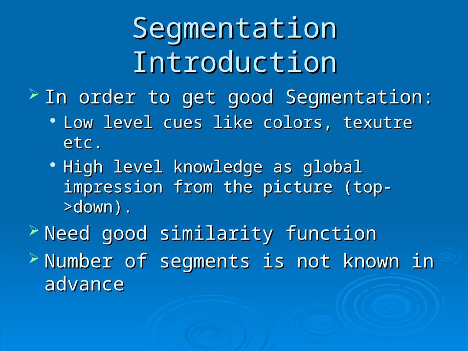
In order to get good Segmentation:In order to get good Segmentation: Low level cues like colors, texutre etc.Low level cues like colors, texutre etc. High level knowledge as global impression High level knowledge as global impression
from the picture (top->down).from the picture (top->down). Need good similarity functionNeed good similarity function Number of segments is not known in Number of segments is not known in
advanceadvance
The Graph partitioning methodThe Graph partitioning method
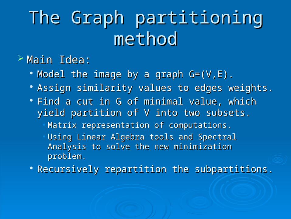
Main Idea:Main Idea: Model the image by a graph G=(V,E).Model the image by a graph G=(V,E). Assign similarity values to edges weights.Assign similarity values to edges weights. Find a cut in G of minimal value, which yield Find a cut in G of minimal value, which yield
partition of V into two subsets.partition of V into two subsets.• Matrix representation of computations.Matrix representation of computations.• Using Linear Algebra tools and Spectral Analysis Using Linear Algebra tools and Spectral Analysis
to solve the new minimization problem.to solve the new minimization problem. Recursively repartition the subpartitions.Recursively repartition the subpartitions.

Graph ModelingGraph Modeling
The Graph G=(V,E)The Graph G=(V,E) Nodes:Nodes:
• PixelsPixels• Some other higher level featuresSome other higher level features
Edges:Edges:• Between every pair of nodes in VBetween every pair of nodes in V
WeightsWeights::• Weight w(i,j) is function of similarity between node Weight w(i,j) is function of similarity between node
i and j.i and j.

Graph ModelingGraph Modeling
Objective Objective Partition the set of vertices into disjoint setsPartition the set of vertices into disjoint sets
Number of segments m is not known.Number of segments m is not known. Cut:Cut:
• Case of m=2, Bi-partition of V into A and B:Case of m=2, Bi-partition of V into A and B:The Cut Value is:The Cut Value is:
• The optimal cut is the one that minimizes its valueThe optimal cut is the one that minimizes its value
1 2 1{ , ,..., }: ,
m
m i j iiV V V i j V V V V
,
( , ) ( , )u A v B
cut A B w u v
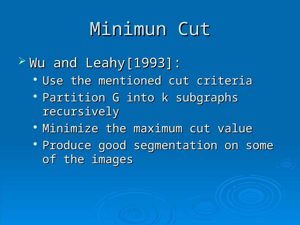
Minimun CutMinimun Cut
Wu and Leahy[1993]:Wu and Leahy[1993]: Use the mentioned cut criteriaUse the mentioned cut criteria Partition G into k subgraphs recursivelyPartition G into k subgraphs recursively Minimize the maximum cut valueMinimize the maximum cut value Produce good segmentation on some of the Produce good segmentation on some of the
imagesimages

Min Cut - The ProblemMin Cut - The Problem
It is not the best cut !It is not the best cut ! Favors cutting small sets of isolated nodes:Favors cutting small sets of isolated nodes:

Normalized Cut [Shi,Malick,1997]Normalized Cut [Shi,Malick,1997]
Normalize the cut value with the volume of Normalize the cut value with the volume of the partition:the partition:
Where Where
( , ) ( , )( , )
( , ) ( , )
cut A B cut A BNcut A B
asso A V asso B V
,
( , ) ( , )u A v V
asso A V w u v

Normalized CutNormalized Cut
Properties:Properties: Sets with weak connections Sets with weak connections Get low Ncut value. Get low Ncut value. High Association within Sets High Association within Sets Get low Ncut value. Get low Ncut value. But - small sets are panalized with high Ncut value.But - small sets are panalized with high Ncut value.
( , ) ( , )( , )
( , ) ( , )
cut A B cut A BNcut A B
asso A V asso B V
,
( , ) ( , )u A v V
asso A V w u v

Normalized AssociationNormalized Association
Normalized Association:Normalized Association:
Naturally related criterions:Naturally related criterions:
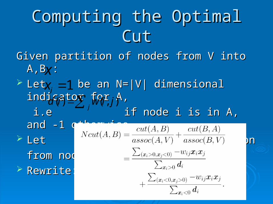
Computing the Optimal CutComputing the Optimal Cut
Given partition of nodes from V into A,B :Given partition of nodes from V into A,B : Let be an N=|V| dimensional indicator for A,Let be an N=|V| dimensional indicator for A,
i.ei.e if node i is in A, and -1 otherwise if node i is in A, and -1 otherwise Let Let be the total connection be the total connection
from node i to all other nodes.from node i to all other nodes. Rewrite:Rewrite:
1ix x
( ) ( , )j
d i w i j

Computing the Optimal CutComputing the Optimal Cut
Objective: TransformObjective: Transform
into Rayleigh’s Quotient-like expression:into Rayleigh’s Quotient-like expression:

Matrix RepresentationMatrix Representation Let D be an N x N diagonal matrix Let D be an N x N diagonal matrix
with d on its diagonal:with d on its diagonal:
Let W be an N x N symmetrical affinity matrix withLet W be an N x N symmetrical affinity matrix with
1
2
0 0
0
0
0 0 N
d
dD
d
( , ) ijW i j w
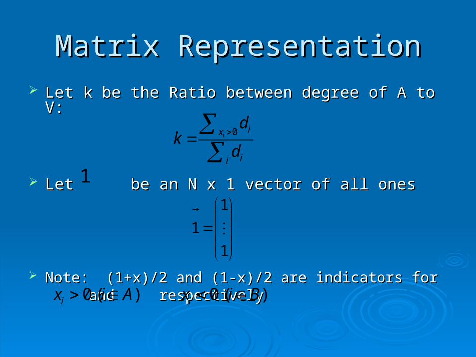
Matrix RepresentationMatrix Representation Let k be the Ratio between degree of A to V:Let k be the Ratio between degree of A to V:
Let be an N x 1 vector of all onesLet be an N x 1 vector of all ones
Note: (1+x)/2 and (1-x)/2 are indicators forNote: (1+x)/2 and (1-x)/2 are indicators for andand respectively respectively0 ( )ix i A
0iix
ii
dk
d
1
1
1
1
0 ( )ix i B
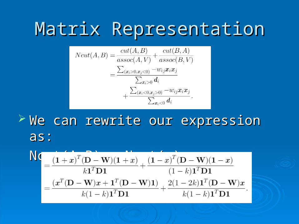
Matrix RepresentationMatrix Representation
We can rewrite our expression as:We can rewrite our expression as:
Ncut(A,B) = Ncut(x) =Ncut(A,B) = Ncut(x) =
Matrix RepresentationMatrix Representation
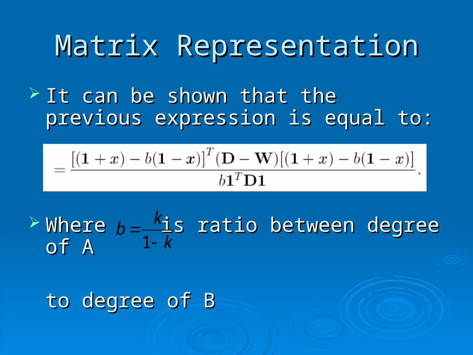
It can be shown that the previous It can be shown that the previous expression is equal to:expression is equal to:
Where Where is ratio between degree of is ratio between degree of A A
to degree of Bto degree of B
1
kb
k
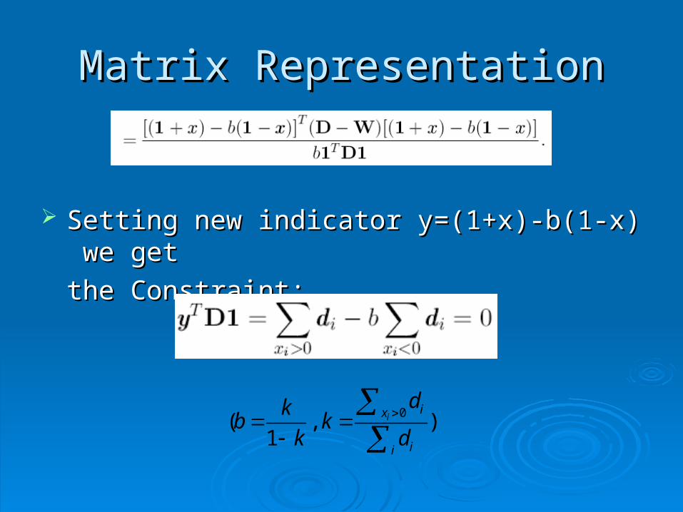
Matrix RepresentationMatrix Representation
Setting new indicator y=(1+x)-b(1-x)Setting new indicator y=(1+x)-b(1-x) we get we get
the Constraint:the Constraint:
0( , )1
iix
ii
dkb k
k d

Matrix RepresentationMatrix Representation
Denominator:Denominator:

Finding the MinimumFinding the Minimum
Putting the last two expression together we getPutting the last two expression together we getthe Rayleigh’s quotient:the Rayleigh’s quotient:
With the conditions: With the conditions: Minimum achieved by finding the minimal Eigenvalue of Minimum achieved by finding the minimal Eigenvalue of
the system(1) (relaxing y to take on real values)the system(1) (relaxing y to take on real values)
Corresponding Eigenvector will be in fact indicator vector Corresponding Eigenvector will be in fact indicator vector for nodes in the segment (A)for nodes in the segment (A)
{1, } 1 0Tiy b and y D

Finding the MinimumFinding the Minimum
But – we have two constraints:But – we have two constraints:
We’ll see that the first one is satisfied:We’ll see that the first one is satisfied: Replacing y byReplacing y by we get the standard we get the standard
eigensystem (2): eigensystem (2):
is an eigenvector of it,with an eigenvalue is an eigenvector of it,with an eigenvalue
of 0.of 0. Since the Laplaician matrix (D-W) is symmetric semi-Since the Laplaician matrix (D-W) is symmetric semi-
positive definite, so that the new system positive definite, so that the new system
1 0Ty D {1, }iy b
12
z D y
12
0 1z D
Finding the MinimumFinding the Minimum
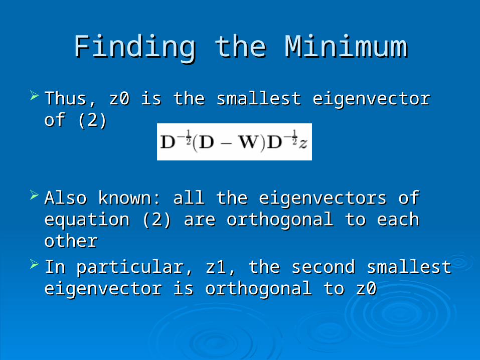
Thus, z0 is the smallest eigenvector of (2)Thus, z0 is the smallest eigenvector of (2)
Also known: all the eigenvectors of Also known: all the eigenvectors of equation (2) are orthogonal to each otherequation (2) are orthogonal to each other
In particular, z1, the second smallest In particular, z1, the second smallest eigenvector is orthogonal to z0eigenvector is orthogonal to z0

Finding the MinimumFinding the Minimum
In terms of our original systemIn terms of our original system))1):1): Is the smallest eigenvector with Is the smallest eigenvector with Where y1 is the 2Where y1 is the 2ndnd
smallest smallest
eigenvector of (1)eigenvector of (1)
The 1The 1stst constraint is automatically satisfied: constraint is automatically satisfied:
0 1y
0
1 0 1 10 T Tz z y D
1 0Ty D
Finding the MinimumFinding the Minimum
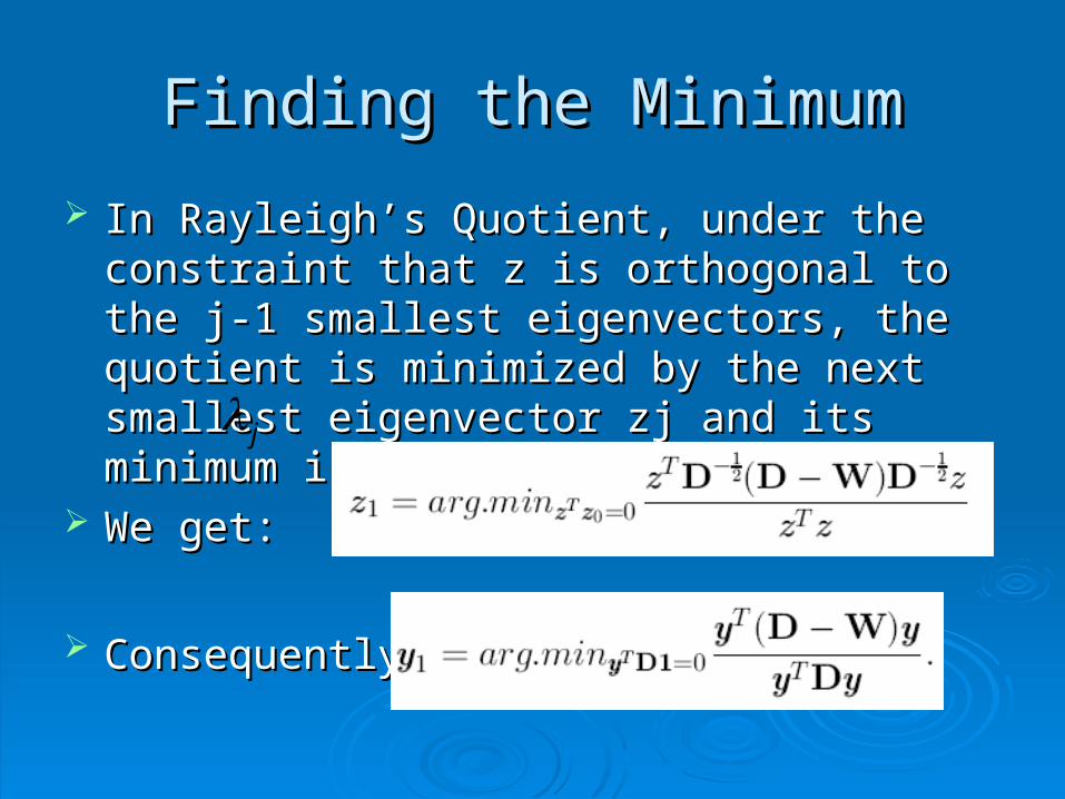
In Rayleigh’s Quotient, under the constraint that In Rayleigh’s Quotient, under the constraint that z is orthogonal to the j-1 smallest eigenvectors, z is orthogonal to the j-1 smallest eigenvectors, the quotient is minimized by the next smallest the quotient is minimized by the next smallest eigenvector zj and its minimum is the eigen eigenvector zj and its minimum is the eigen value value
We get:We get:
Consequently:Consequently:
j

Finding the MinimumFinding the Minimum
Conclusion: the 2Conclusion: the 2ndnd smallest eigenvector of (1) smallest eigenvector of (1)
is the real solution to our Normalized Cut is the real solution to our Normalized Cut problem.problem.
What about the 2What about the 2ndnd constraint that y takes on constraint that y takes on discrete values??discrete values?? Solving the discrete problem is NP-CompleteSolving the discrete problem is NP-Complete Solution – approximate the continuous solution by Solution – approximate the continuous solution by
splitting the vector coordinates at different splitting the vector coordinates at different thresholds, choosing the one that gives the best thresholds, choosing the one that gives the best NCut value.NCut value.
{1, }iy b
ComplexityComplexity
Wait! Wait!
What about the original graph problem ?What about the original graph problem ? MinCut – Has Polynomial-Time algorithmMinCut – Has Polynomial-Time algorithm
by the MaxFlow algorithm. by the MaxFlow algorithm. Impractical for imagesImpractical for images
Normalized Cut – NP-CompleteNormalized Cut – NP-Complete Need fast approximationsNeed fast approximations
5( )O n

ComplexityComplexity
Solving standard eigenvalue problem Solving standard eigenvalue problem Impractical for segmenting large number of Impractical for segmenting large number of
pixelspixels Special properties of our problem:Special properties of our problem:
The graph often locally connected=>sparse The graph often locally connected=>sparse matrixmatrix
Only the top eigenvectors are neededOnly the top eigenvectors are needed Low precision requirementsLow precision requirements
Using Lanczos eigensolver - Using Lanczos eigensolver -
3( )O n
112( )O n

RepartitioningRepartitioning
Recursively apply the above method to each of Recursively apply the above method to each of the partitionsthe partitions Subject to some “stability” criteria:Subject to some “stability” criteria:
• Create sub partitions by varying the splitting point around the Create sub partitions by varying the splitting point around the optimal value and check if Ncut value change muchoptimal value and check if Ncut value change much
Until certain Ncut threshold exceededUntil certain Ncut threshold exceeded
Another approach: Use high order eigenvectorsAnother approach: Use high order eigenvectors Pros: more discriminative informationPros: more discriminative information Cons: according to Shi&Malik, Approximation error Cons: according to Shi&Malik, Approximation error
accumulates with every eigenvector takenaccumulates with every eigenvector taken

Summary of the AlgorithmSummary of the Algorithm
1.1. Given features, construct the graphGiven features, construct the graph2.2. SolveSolve for eigenvectors with the for eigenvectors with the
smallest eigenvaluessmallest eigenvalues3.3. Use the eigenvector with the 2Use the eigenvector with the 2ndnd smallest smallest
eigenvalue to bipartition the grapheigenvalue to bipartition the graph Find the splitting point that minimizes NcutFind the splitting point that minimizes Ncut
4.4. Check stability and Ncut threshold to decide Check stability and Ncut threshold to decide whether whether to divide the current partition.to divide the current partition.
5.5. Recursively repartition the segmented parts if Recursively repartition the segmented parts if necessarynecessary

ExperimentsExperiments
Pixels as Graph nodesPixels as Graph nodes Weight Function:Weight Function:
X(i) – Spatial location of node IX(i) – Spatial location of node I F(i) – Feature vector based on Intensity, Color F(i) – Feature vector based on Intensity, Color
or Texture information at node i or Texture information at node i
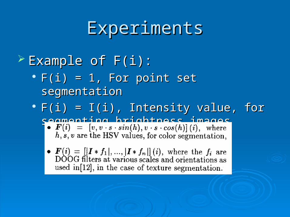
ExperimentsExperiments
Example of F(i):Example of F(i): F(i) = 1, For point set segmentationF(i) = 1, For point set segmentation F(i) = I(i), Intensity value, for segmenting F(i) = I(i), Intensity value, for segmenting
brightness imagesbrightness images

ExperimentsExperiments
Point setPoint set
Taken from [1]

ExperimentsExperiments
Synthetic image of cornerSynthetic image of corner
Taken from [1]

ExperimentsExperiments
Taken from [1]

ExperimentsExperiments
““Color” imageColor” image
Taken from [1]
ExperimentsExperiments
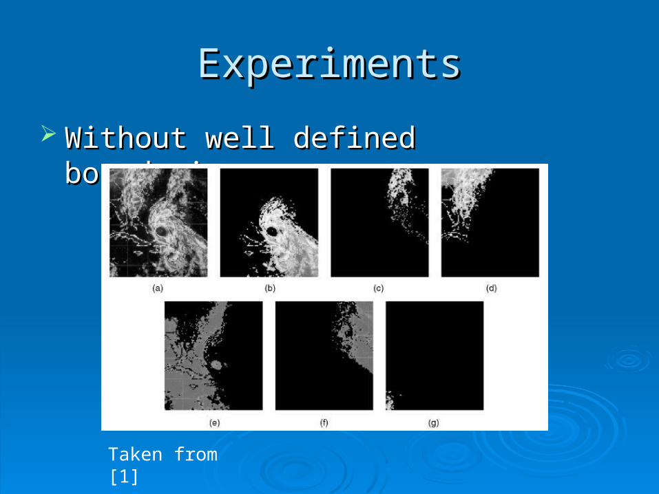
Without well defined boundaries:Without well defined boundaries:
Taken from [1]
ExperimentsExperiments
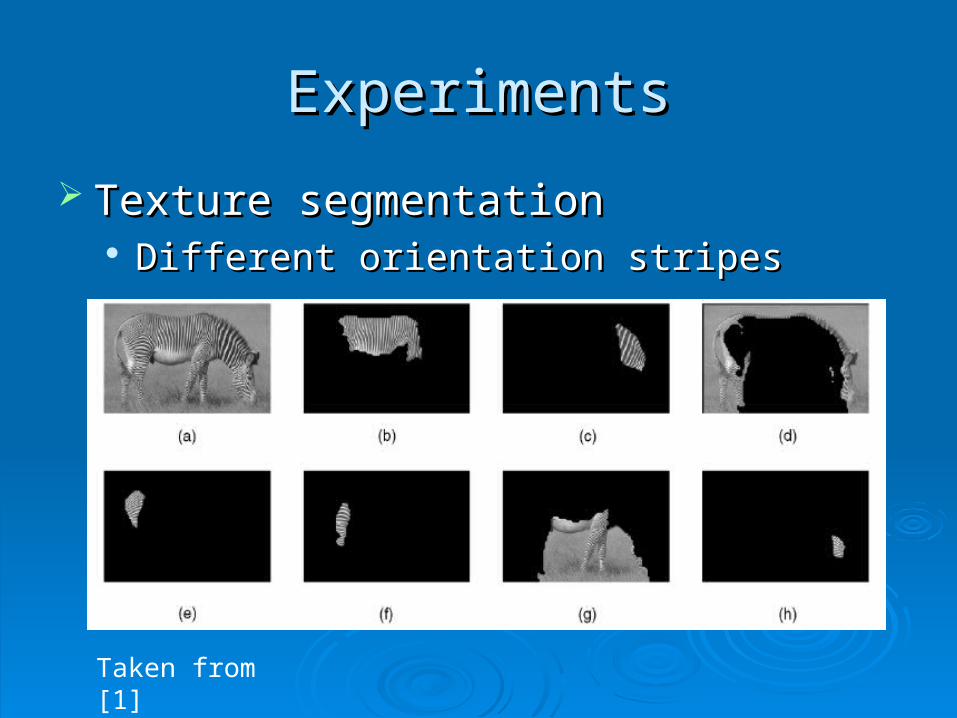
Texture segmentationTexture segmentation Different orientation stripesDifferent orientation stripes
Taken from [1]

A little bit moreA little bit more....
Taken from [2]

A little bit moreA little bit more....
High order eigenvectorsHigh order eigenvectors
Taken from [2]

High order eigenvectorsHigh order eigenvectors
Taken from [2]

11stst Vs 2 Vs 2ndnd Eigenvectors Eigenvectors
Taken from [3]

SummerySummery Treat the problem as graph partitioningTreat the problem as graph partitioning The new idea:The new idea:
Normalized Cut instead of Regular CutNormalized Cut instead of Regular Cut NCut criteria measures both:NCut criteria measures both:
Dissimilarity between groupsDissimilarity between groups Similarity within a groupSimilarity within a group
Global impression extraction of the imageGlobal impression extraction of the image Spectral Analysis in favor of segmenting imagesSpectral Analysis in favor of segmenting images Generalized eigenvalue system gives real Generalized eigenvalue system gives real
solution=>”segmenting” this data provide solution=>”segmenting” this data provide clustering of the original imageclustering of the original image

Thanks!Thanks!