Nonstationary covariance structures II

NRCSE

Drawbacks with deformation approach

Oversmoothing of large areas

Local deformations not local part of global fits

Covariance shape does not change over space

Limited class of nonstationary covariances

Nonstationary spatial covariance:

Basic idea: the parameters of a local variogram model–-nugget, range, sill, and anisotropy–vary spatially.

Consider some pictures of applications from recent methodology publications.

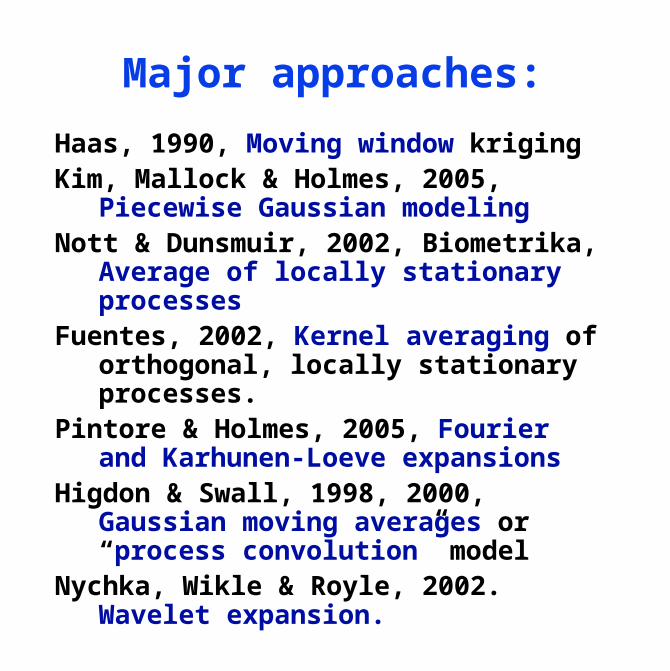
Major approaches:

Haas, 1990, Moving window krigingKim, Mallock & Holmes, 2005, Piecewise

Gaussian modelingNott & Dunsmuir, 2002, Biometrika,

Average of locally stationary processesFuentes, 2002, Kernel averaging of

orthogonal, locally stationary processes.

Pintore & Holmes, 2005, Fourier and Karhunen-Loeve expansions

Higdon & Swall, 1998, 2000, Gaussian moving averages or “process convolution” model

Nychka, Wikle & Royle, 2002. Wavelet expansion.

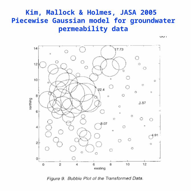
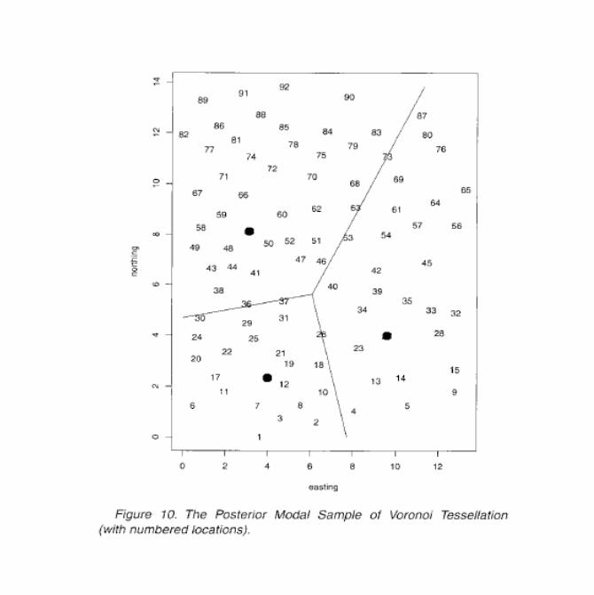
Kim, Mallock & Holmes, JASA 2005 Piecewise Gaussian model for groundwater

permeability data

QuickTime™ and a decompressor

are needed to see this picture.

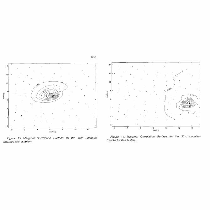
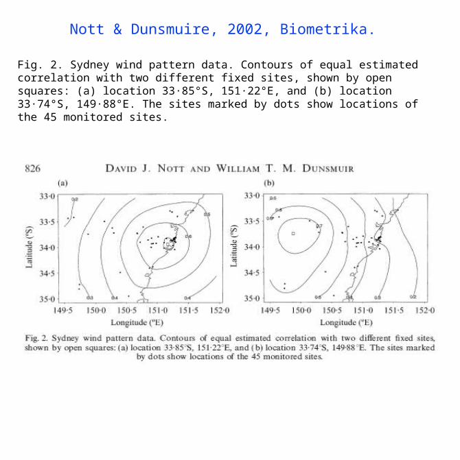
Fig. 2. Sydney wind pattern data. Contours of equal estimated correlation with two different fixed sites, shown by open squares: (a) location 33·85°S, 151·22°E, and (b) location 33·74°S, 149·88°E. The sites marked by dots show locations of the 45 monitored sites.

Nott & Dunsmuire, 2002, Biometrika.

QuickTime™ and a decompressor

are needed to see this picture.

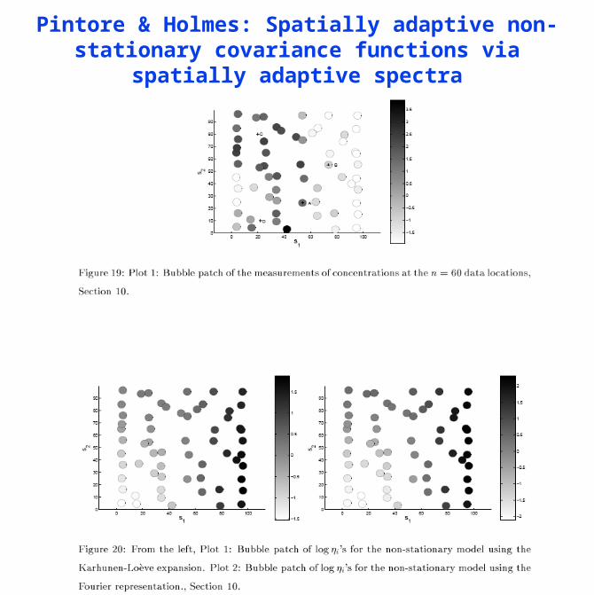
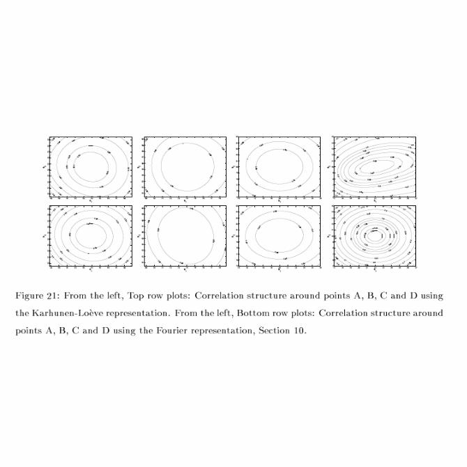
Pintore & Holmes: Spatially adaptive non-stationary covariance functions via spatially adaptive spectra

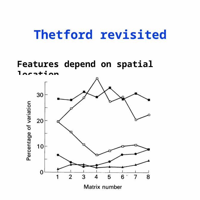
Thetford revisited

Features depend on spatial location

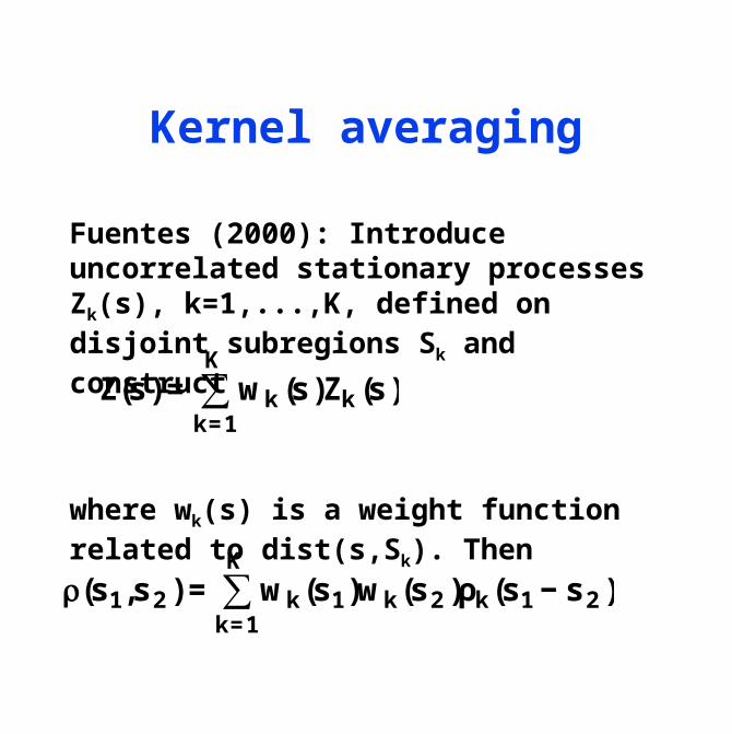
Kernel averaging

Fuentes (2000): Introduce uncorrelated stationary processes Zk(s), k=1,...,K, defined on disjoint subregions Sk and construct

where wk(s) is a weight function related to dist(s,Sk). Then

€

Z(s) = wk (s)Zk (s)k=1

K

∑

€

ρ(s1,s2 ) = wk(s1)wk(s2 )ρkk=1

K

∑ (s1 − s2 )

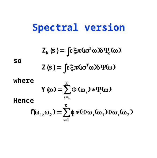
Spectral version

so

where

Hence

Zk (s) = exp(isTω)dYk∫ (ω)

Z(s) = exp(isTω)dY(ω)∫

Y(ω) = F (wi )∗Yi (ω)

i=1

K

∑

f(ω1,ω2 ) = fi

i=1

K

∑ ∗(F wi (ω1)F wi (ω2 )

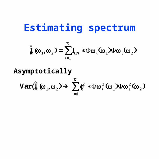
Estimating spectrum

Asymptotically

IN (ω1,ω2 ) = Ii,N ∗F wi (ω1)F wi (ω2 )

i=1

K

∑

Var(IN (ω1,ω2 ) → fi

2 ∗F wi2 (ω1)F wi

2 (ω2 )i=1

K

∑

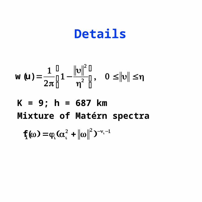
Details

K = 9; h = 687 km

Mixture of Matérn spectra

w(u) =12π

1−u

2

h2

⎛

⎝⎜

⎞

⎠⎟ , 0 ≤ u ≤h

fi (ω) =φi (α i2 + ω 2 )−νi−1

An example

QuickTime™ and aTIFF (LZW) decompressor

are needed to see this picture.

Models-3 output, 81x87 grid, 36km x 36km. Hourly averaged nitric acid concentration week of 950711.

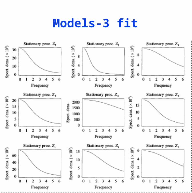
Models-3 fit

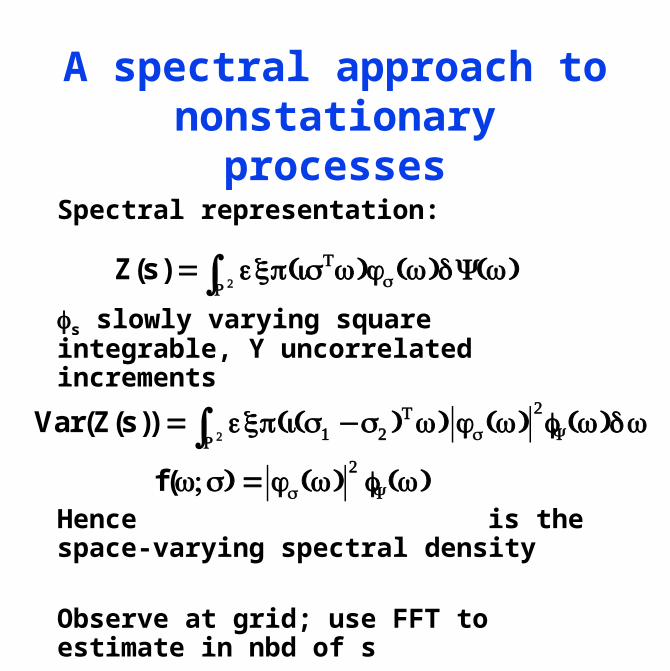
A spectral approach to nonstationary processes

Spectral representation:

s slowly varying square integrable, Y uncorrelated increments

Hence is the space-varying spectral density

Observe at grid; use FFT to estimate in nbd of s

Z(s) = exp(isTω)φs (ω)dY(ω)R2∫

Var(Z(s)) = exp(i(s1 −s2 )Tω) φs (ω)

2

R2∫ fY (ω)dω

f(ω;s) = φs (ω)2fY (ω)

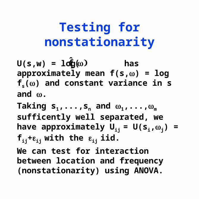
Testing for nonstationarity

U(s,w) = log has approximately mean f(s,ω) = log fs(ω) and constant variance in s and ω.

Taking s1,...,sn and ω1,...,ωm sufficently well separated, we have approximately Uij = U(si,ωj) = fij+ij with the ij iid.

We can test for interaction between location and frequency (nonstationarity) using ANOVA.

fs (ω)

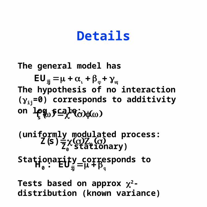
Details

The general model has

The hypothesis of no interaction (ij=0) corresponds to additivity on log scale:

(uniformly modulated process:

Z0 stationary)

Stationarity corresponds to

Tests based on approx 2-distribution (known variance)

EUij =μ + α i + β j + ij

fs (ω) =c2 (s)f(ω)

Z(s) =c(s)Z0 (s)

H0 : EUij =μ +β j

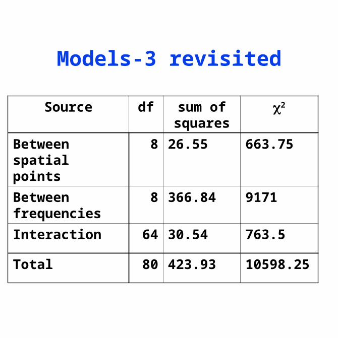
Models-3 revisited

Source df sum of squares

2

Between spatial points

8 26.55 663.75

Between frequencies

8 366.84 9171

Interaction 64 30.54 763.5

Total 80 423.93 10598.25

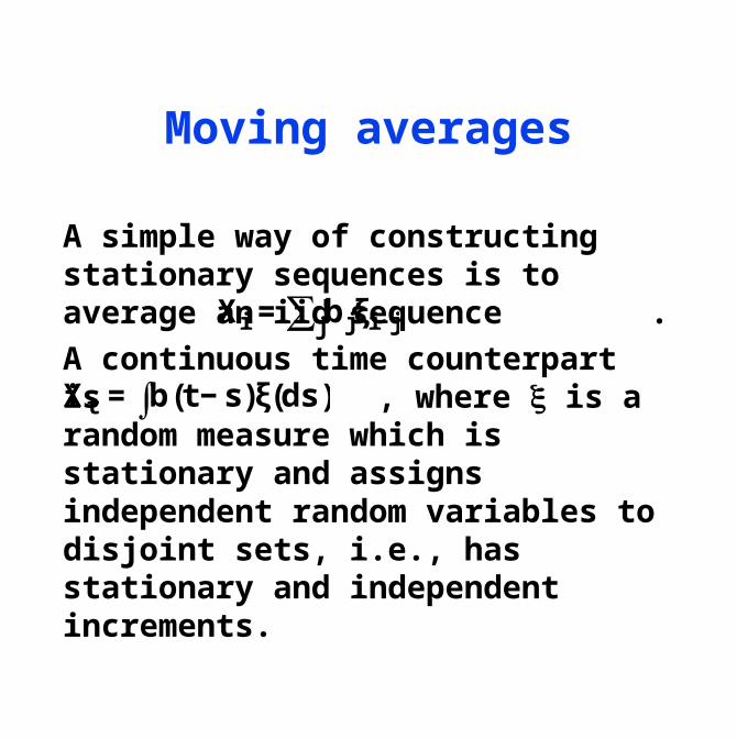
Moving averages

A simple way of constructing stationary sequences is to average an iid sequence .

A continuous time counterpart is , where is a random

measure which is stationary and assigns independent random variables to disjoint sets, i.e., has stationary and independent increments.

Xi = bjξi−jj∑

Xt = b(t−s)ξ(ds)∫

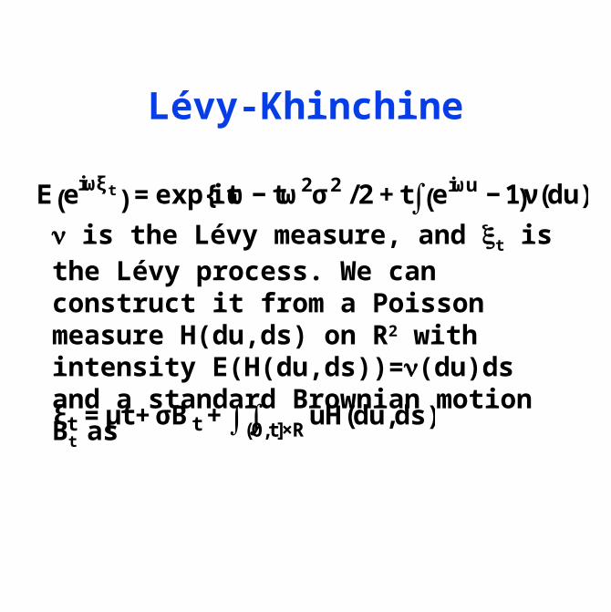
Lévy-Khinchine

ν is the Lévy measure, and t is the Lévy process. We can construct it from a Poisson measure H(du,ds) on R2 with intensity E(H(du,ds))=ν(du)ds and a standard Brownian motion Bt as

E eiωξt( )=exp{itω−tω2σ2 /2+t eiωu−1( )∫ ν(du)

ξt =μt+σBt+ uH(du,ds)(0,t]×R∫∫

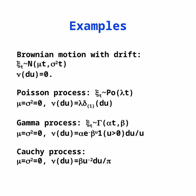
Examples

Brownian motion with drift: t~N(μt,2t)ν(du)=0.

Poisson process: t~Po(t)μ=2=0, ν(du)={1}(du)

Gamma process: t~(αt,β)μ=2=0, ν(du)=αe-βu1(u>0)du/u

Cauchy process:μ=2=0, ν(du)=βu-2du/π

Spatial moving averages

We can replace R for t with R2 (or a general metric space)

We can replace R for s with R2 (or a general metric space)

We can replace b(t-s) by bt(s) to relax stationarity

We can let the intensity measure for H be an arbitrary measure ν(ds,du)

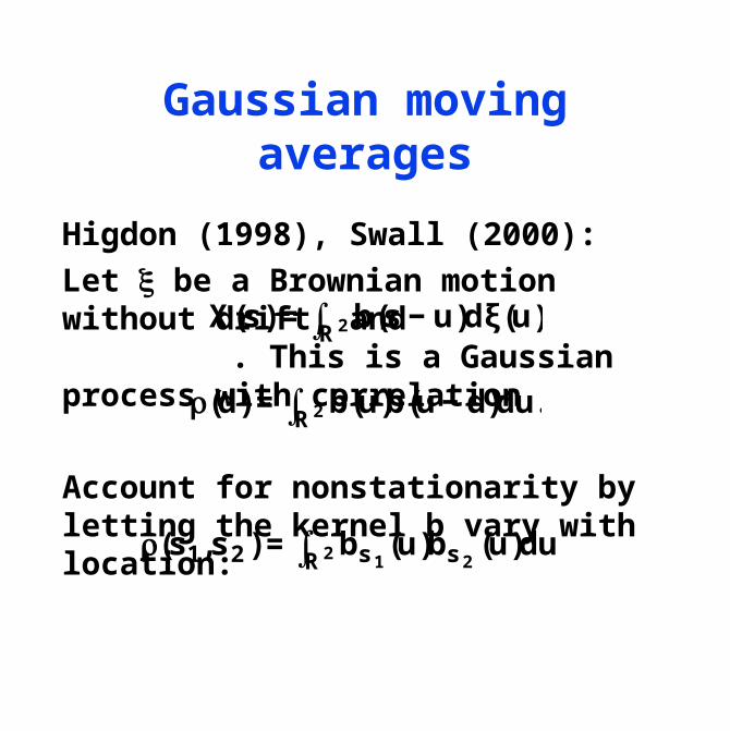
Gaussian moving averages

Higdon (1998), Swall (2000):

Let be a Brownian motion without drift, and . This is a Gaussian process with correlation

Account for nonstationarity by letting the kernel b vary with location:

€

X(s) = b(s − u)dξ (u)R2∫

€

ρ(d) = b(u)R2∫ b(u − d)du.

€

ρ(s1,s2 ) = bs 1R2∫ (u)bs 2(u)du

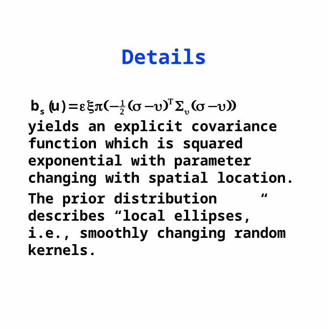
Details

yields an explicit covariance function which is squared exponential with parameter changing with spatial location.

The prior distribution describes “local ellipses,” i.e., smoothly changing random kernels.

bs (u) =exp(−12 (s −u)TΣu(s −u))

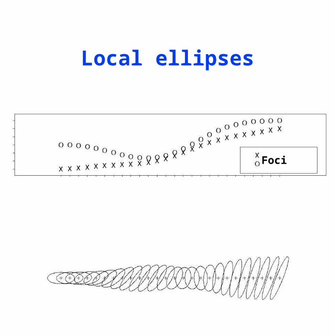
Local ellipses

Foci

Prior parametrization

Foci chosen independently Gaussian with isotropic squared exponential covariance

Another parameter describes the range of influence of a given ellipse. Prior gamma.

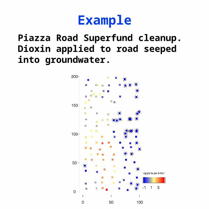
ExamplePiazza Road Superfund cleanup. Dioxin applied to road seeped into groundwater.

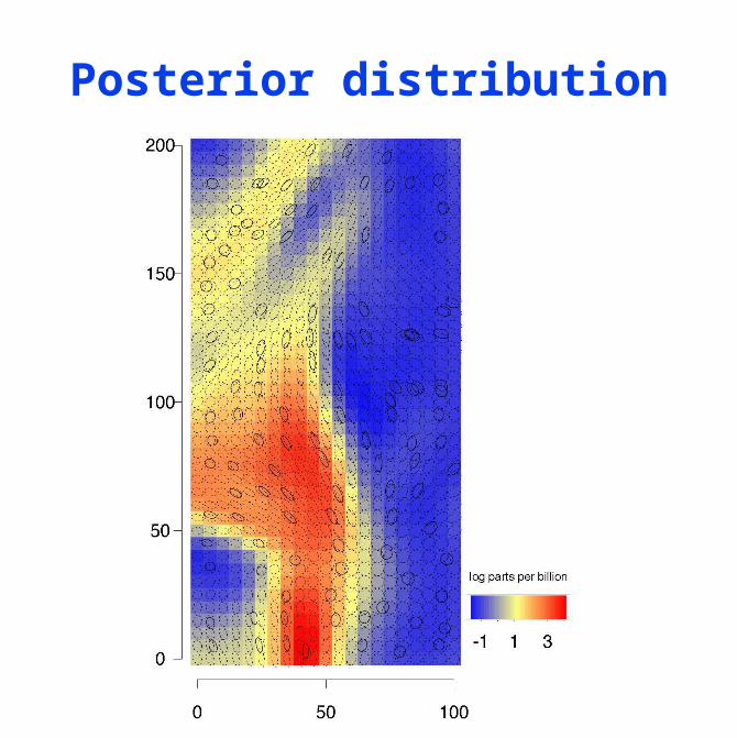
Posterior distribution