nonlinear state estimation and modeling of a helicopter uav
TRANSCRIPT

University of Alberta
Nonlinear State Estimation and Modeling of a Helicopter UAV
by
Martin Barczyk
A thesis submitted to the Faculty of Graduate Studies and Researchin partial fulfillment of the requirements for the degree of
Doctor of Philosophy
in
Control Systems
Department of Electrical and Computer Engineering
c©Martin BarczykSpring 2012
Edmonton, Alberta
Permission is hereby granted to the University of Alberta Libraries to reproduce single copies ofthis thesis and to lend or sell such copies for private, scholarly or scientific research purposes only.Where the thesis is converted to, or otherwise made available in digital form, the University of
Alberta will advise potential users of the thesis of these terms.
The author reserves all other publication and other rights in association with the copyright in thethesis and, except as herein before provided, neither the thesis nor any substantial portion thereofmay be printed or otherwise reproduced in any material form whatsoever without the author’s
prior written permission.

Abstract
Experimentally-validated nonlinear flight control of a helicopter UAV has two nec-
essary conditions: an estimate of the vehicle’s states from noisy multirate output
measurements, and a nonlinear dynamics model with minimum complexity, physi-
cally controllable inputs and experimentally identified parameter values. This thesis
addresses both these objectives for the Applied Nonlinear Controls Lab (ANCL)’s
helicopter UAV project. A magnetometer-plus-GPS aided Inertial Navigation Sys-
tem (INS) for outdoor flight as well as an Attitude and Heading Reference System
(AHRS) for indoor testing are designed, implemented and experimentally validated
employing an Extended Kalman Filter (EKF), using a novel calibration technique
for the magnetometer aiding sensor added to remove the limitations of an earlier
GPS-only aiding design. Next the recently-developed nonlinear observer design
methodology of invariant observers is adapted to the aided INS and AHRS exam-
ples, employing a rotation matrix representation for the state manifold to obtain
designs amenable to global stability analysis, obtaining a direct nonlinear design
for gains of the AHRS observer, modifying the previously-proposed Invariant EKF
systematic method for computing gains, and culminating in simulation and exper-
imental validation of the observers. Lastly a nonlinear control-oriented model of
the helicopter UAV is derived from first principles, using a rigid-body dynamics
formulation augmented with models of the on-board subsystems: main rotor forces
and blade flapping dynamics, the Bell-Hiller system and flybar flapping dynamics,
tail rotor forces, tail gyro unit, engine and rotor speed, servo operation, fuselage
drag, and tail stabilizer forces. The parameter values in the resulting models are
identified experimentally. Using these the model is further simplified to be tractable
for model-based control design.

Table of Contents
1 Introduction 1
1.1 Background . . . . . . . . . . . . . . . . . . . . . . . . . . . . . . . . 11.1.1 Motivation of Research . . . . . . . . . . . . . . . . . . . . . 3
1.2 Literature Survey . . . . . . . . . . . . . . . . . . . . . . . . . . . . . 41.2.1 Aided Navigation . . . . . . . . . . . . . . . . . . . . . . . . . 41.2.2 Invariant Observers . . . . . . . . . . . . . . . . . . . . . . . 41.2.3 Helicopter Modeling and Identification . . . . . . . . . . . . . 5
1.3 Outline of Thesis . . . . . . . . . . . . . . . . . . . . . . . . . . . . . 51.3.1 Statement of Contributions . . . . . . . . . . . . . . . . . . . 6
2 Mathematical Preliminaries 8
2.1 Rotation Matrices . . . . . . . . . . . . . . . . . . . . . . . . . . . . 82.2 Cross-Product and Skew-Symmetric Matrices . . . . . . . . . . . . . 102.3 Rotation Kinematics . . . . . . . . . . . . . . . . . . . . . . . . . . . 112.4 Navigation Dynamics . . . . . . . . . . . . . . . . . . . . . . . . . . . 132.5 Parameterizing the Rotation Matrix . . . . . . . . . . . . . . . . . . 152.6 Euler Angles Parametrization . . . . . . . . . . . . . . . . . . . . . . 182.7 Quaternions . . . . . . . . . . . . . . . . . . . . . . . . . . . . . . . . 222.8 Earth’s Magnetic Field . . . . . . . . . . . . . . . . . . . . . . . . . . 28
2.8.1 Computing Yaw . . . . . . . . . . . . . . . . . . . . . . . . . 302.9 Magnetometer Calibration . . . . . . . . . . . . . . . . . . . . . . . . 31
3 Extended Kalman Filter Design for Aided Navigation 35
3.1 Overview of EKF . . . . . . . . . . . . . . . . . . . . . . . . . . . . . 353.2 EKF Design . . . . . . . . . . . . . . . . . . . . . . . . . . . . . . . . 36
3.2.1 Complementary Filter Topology . . . . . . . . . . . . . . . . 363.2.2 Sensor Models . . . . . . . . . . . . . . . . . . . . . . . . . . 383.2.3 Dynamics and Output Equations . . . . . . . . . . . . . . . . 393.2.4 Numerical Integration . . . . . . . . . . . . . . . . . . . . . . 403.2.5 Linearized Error Dynamics . . . . . . . . . . . . . . . . . . . 423.2.6 Observability Analysis . . . . . . . . . . . . . . . . . . . . . . 453.2.7 Discretization . . . . . . . . . . . . . . . . . . . . . . . . . . . 483.2.8 Kalman Filter . . . . . . . . . . . . . . . . . . . . . . . . . . . 513.2.9 Extended Kalman Filter . . . . . . . . . . . . . . . . . . . . . 523.2.10 EKF Implementation . . . . . . . . . . . . . . . . . . . . . . 523.2.11 Initialization . . . . . . . . . . . . . . . . . . . . . . . . . . . 54
3.3 AHRS Testing . . . . . . . . . . . . . . . . . . . . . . . . . . . . . . 56

3.3.1 Simulation Results . . . . . . . . . . . . . . . . . . . . . . . . 563.3.2 Experimental Results . . . . . . . . . . . . . . . . . . . . . . 57
3.4 Aided INS Testing . . . . . . . . . . . . . . . . . . . . . . . . . . . . 583.4.1 Simulation Results . . . . . . . . . . . . . . . . . . . . . . . . 583.4.2 Experimental Ground Test Results . . . . . . . . . . . . . . . 613.4.3 Experimental Flight Results . . . . . . . . . . . . . . . . . . . 64
4 Invariant Observer Design for Aided Navigation 69
4.1 Overview . . . . . . . . . . . . . . . . . . . . . . . . . . . . . . . . . 694.2 Motivating Example . . . . . . . . . . . . . . . . . . . . . . . . . . . 704.3 System Symmetries . . . . . . . . . . . . . . . . . . . . . . . . . . . . 72
4.3.1 Lie Group Actions . . . . . . . . . . . . . . . . . . . . . . . . 744.4 AHRS symmetries . . . . . . . . . . . . . . . . . . . . . . . . . . . . 75
4.4.1 Ground frame symmetries . . . . . . . . . . . . . . . . . . . . 754.4.2 Combined symmetries . . . . . . . . . . . . . . . . . . . . . . 76
4.5 Aided INS Symmetries . . . . . . . . . . . . . . . . . . . . . . . . . . 784.6 Invariant Observer Theory . . . . . . . . . . . . . . . . . . . . . . . . 82
4.6.1 Invariants and Moving Frame . . . . . . . . . . . . . . . . . . 824.6.2 Invariant Frame . . . . . . . . . . . . . . . . . . . . . . . . . 854.6.3 Invariant Observer, Invariant Output Error . . . . . . . . . . 87
4.7 Invariant Observer Design . . . . . . . . . . . . . . . . . . . . . . . . 914.7.1 Invariant AHRS Design . . . . . . . . . . . . . . . . . . . . . 914.7.2 Invariant Aided INS Design . . . . . . . . . . . . . . . . . . . 97
4.8 Nonlinear Observer Gain Design . . . . . . . . . . . . . . . . . . . . 1044.9 Invariant Extended Kalman Filter . . . . . . . . . . . . . . . . . . . 106
4.9.1 Invariant EKF Overview . . . . . . . . . . . . . . . . . . . . . 1074.9.2 Invariant AHRS EKF design . . . . . . . . . . . . . . . . . . 1084.9.3 Invariant Aided INS EKF design . . . . . . . . . . . . . . . . 113
4.10 Invariant AHRS testing . . . . . . . . . . . . . . . . . . . . . . . . . 1214.10.1 Implementation Details . . . . . . . . . . . . . . . . . . . . . 1214.10.2 Simulation Results . . . . . . . . . . . . . . . . . . . . . . . . 1234.10.3 Experimental Results . . . . . . . . . . . . . . . . . . . . . . 126
4.11 Invariant Aided INS testing . . . . . . . . . . . . . . . . . . . . . . . 1304.11.1 Implementation details . . . . . . . . . . . . . . . . . . . . . . 1304.11.2 Simulation results . . . . . . . . . . . . . . . . . . . . . . . . 1324.11.3 Experimental results . . . . . . . . . . . . . . . . . . . . . . . 135
5 Nonlinear Model of a Helicopter UAV 139
5.1 Overview . . . . . . . . . . . . . . . . . . . . . . . . . . . . . . . . . 1395.2 Rigid-Body Model . . . . . . . . . . . . . . . . . . . . . . . . . . . . 139
5.2.1 Torsional Pendulum . . . . . . . . . . . . . . . . . . . . . . . 1445.2.2 Extended Moment Equation . . . . . . . . . . . . . . . . . . . 146
5.3 Aerodynamics and Subsystem Modeling . . . . . . . . . . . . . . . . 1485.3.1 Main Rotor . . . . . . . . . . . . . . . . . . . . . . . . . . . . 1485.3.2 Rotor Head . . . . . . . . . . . . . . . . . . . . . . . . . . . . 1685.3.3 Tail Rotor . . . . . . . . . . . . . . . . . . . . . . . . . . . . . 1765.3.4 Rotor Speed and Engine . . . . . . . . . . . . . . . . . . . . . 1815.3.5 Servo Commands . . . . . . . . . . . . . . . . . . . . . . . . . 182

5.3.6 Fuselage Drag . . . . . . . . . . . . . . . . . . . . . . . . . . . 1845.3.7 Tail Stabilizers . . . . . . . . . . . . . . . . . . . . . . . . . . 185
5.4 Dynamics Model Summary . . . . . . . . . . . . . . . . . . . . . . . 1885.4.1 Hover Model . . . . . . . . . . . . . . . . . . . . . . . . . . . 189
5.5 Identified Parameter Values . . . . . . . . . . . . . . . . . . . . . . . 191
6 Conclusions 194
6.1 Review of Results . . . . . . . . . . . . . . . . . . . . . . . . . . . . . 1946.1.1 Magnetometer Integration . . . . . . . . . . . . . . . . . . . . 1946.1.2 Invariant Observers . . . . . . . . . . . . . . . . . . . . . . . 1946.1.3 Modeling and Identification . . . . . . . . . . . . . . . . . . . 195
6.2 Future Work . . . . . . . . . . . . . . . . . . . . . . . . . . . . . . . 1966.2.1 Engine-on Noise Characteristics . . . . . . . . . . . . . . . . . 1966.2.2 Nonlinear Gain Design for Invariant Aided INS Observer . . 1976.2.3 Experimental Testing of Nonlinear Model . . . . . . . . . . . 197
Bibliography 198

List of Tables
2.1 Magnetometer Calibration Constants . . . . . . . . . . . . . . . . . . 34
3.1 Identified Noise Parameters – Engine Off [75] . . . . . . . . . . . . . 383.2 Modified Noise Parameters – Engine On . . . . . . . . . . . . . . . . 65
4.1 Engine-on Invariant Aided INS observer parameters . . . . . . . . . 137
List of Figures
1.1 ANCL helicopter UAV in flight [75]; note the underslung avionicsenclosure and tail-mounted GPS antenna . . . . . . . . . . . . . . . 2
2.1 Three-frame schematic; frame origins offset for clarity . . . . . . . . 102.2 Rigid Body Rotation About Fixed Origin . . . . . . . . . . . . . . . 122.3 Body, Navigation and ECEF frames . . . . . . . . . . . . . . . . . . 142.4 Elementary rotations about n1, n2 and n3 . . . . . . . . . . . . . . . 182.5 Roll-Pitch-Yaw sequence of rotations, φ = −π/2, θ = π/2, ψ = π . . 212.6 Alternative Roll-Pitch-Yaw sequence of rotations, φ = −π, θ = π/2,
ψ = π/2 . . . . . . . . . . . . . . . . . . . . . . . . . . . . . . . . . . 212.7 Earth’s Magnetic Field . . . . . . . . . . . . . . . . . . . . . . . . . . 292.8 Magnetometer Calibration, Engine Off: Raw Sensor Readings, Hard-
Iron Compensated, Fully Compensated . . . . . . . . . . . . . . . . . 33
3.1 Topology of AHRS; signal rate inversely proportional to dot spacing 373.2 Topology of Aided INS; signal rate inversely proportional to dot spacing 373.3 AHRS simulation: estimated states (—), reference states (- - -). . . . 563.4 AHRS simulation: error between estimated and reference attitude
angles . . . . . . . . . . . . . . . . . . . . . . . . . . . . . . . . . . . 573.5 AHRS experiment: estimated states (—), Vicon attitudes (- - -). . . . 573.6 AHRS experiment: error between AHRS and Vicon attitudes; ‖ya‖ . 583.7 State Estimates: Simulated Hover . . . . . . . . . . . . . . . . . . . 593.8 State Estimates: Simulated Hover, GPS-only Aiding . . . . . . . . . 593.9 State Estimates: Simulated figure-8 . . . . . . . . . . . . . . . . . . . 603.10 State Estimates: Simulated figure-8, GPS-only Aiding . . . . . . . . 613.11 State Estimation Errors: Simulated figure-8, Mag-plus-GPS vs GPS-
only Aiding . . . . . . . . . . . . . . . . . . . . . . . . . . . . . . . . 613.12 State Estimates: Ground Test, 3-Axis Mag Aiding . . . . . . . . . . 623.13 State Estimates: Ground Test, Yaw-Only Mag Aiding . . . . . . . . 633.14 Magnetometer Calibration Comparison, Ground Test, Yaw-Only Mag
Aiding: Overhead Position; Yaw Angle . . . . . . . . . . . . . . . . . 643.15 State Estimates: Flight Test, 3-Axis Mag Aiding . . . . . . . . . . . 653.16 State Estimates: Flight Test, Yaw-Only Mag Aiding . . . . . . . . . 663.17 Magnetometer Calibration Comparison, Flight Test, 3-Axis Mag Aid-
ing: Estimated Attitude . . . . . . . . . . . . . . . . . . . . . . . . . 67
4.1 Orbits of SO(2) on R2 and cross-section K . . . . . . . . . . . . . . 84

4.2 Invariant AHRS Simulation: Body-Frame Symmetry Observer (4.15)using gains from nonlinear design (left); Invariant EKF (right) . . . 124
4.3 Invariant AHRS Simulation: Ground-Frame Symmetry Observer (4.16)using gains from nonlinear design (left); Invariant EKF (right) . . . 125
4.4 Invariant AHRS Simulation: Comparison of estimation errors . . . . 1264.5 Invariant AHRS Experiment: Body-Frame Symmetry Observer (4.15)
using gains from nonlinear design (left); Invariant EKF (right) . . . 1274.6 Invariant AHRS Experiment: Ground-Frame Symmetry Observer (4.16)
using gains from nonlinear design (left); Invariant EKF (right) . . . 1284.7 Invariant AHRS Experiment: Comparison of attitude estimation errors1294.8 Body-Frame Invariant Aided INS: Simulated Hover . . . . . . . . . . 1334.9 Ground-Frame Invariant Aided INS: Simulated Hover . . . . . . . . 1334.10 Body-Frame Invariant Aided INS: Simulated Figure-8 flight . . . . . 1344.11 Ground-Frame Invariant Aided INS: Simulated Figure-8 flight . . . . 1344.12 Invariant Aided INS: Simulated Figure-8 flight estimation errors: Body-
frame symmetry; Ground-frame symmetry . . . . . . . . . . . . . . . 1344.13 Body-Frame Invariant Aided INS: Experimental engine-off walk . . . 1354.14 Ground-Frame Invariant Aided INS: Experimental engine-off walk . 1354.15 Invariant Aided INS: Experimental engine-off walk comparison: Body-
frame symmetry; Ground-frame symmetry . . . . . . . . . . . . . . . 1364.16 Body-Frame Invariant Aided INS: Experimental engine-on hover . . 1374.17 Ground-Frame Invariant Aided INS: Experimental engine-on hover . 1384.18 Invariant Aided INS: Pre-takeoff estimated position zoom-in view . . 138
5.1 Helicopter Model: Overall View [59] . . . . . . . . . . . . . . . . . . 1405.2 Navigation and Body Frames on Helicopter . . . . . . . . . . . . . . 1405.3 Helicopter UAV with identified CM location . . . . . . . . . . . . . . 1445.4 Torsional pendulum schematic . . . . . . . . . . . . . . . . . . . . . 1445.5 Geometry of support cable; disk rotated by θ . . . . . . . . . . . . . 1455.6 Experimental measurement of J using a torsional pendulum [53]:
pitch axis, roll axis. . . . . . . . . . . . . . . . . . . . . . . . . . . . . 1465.7 Rigid body with body frame fixed at arbitrary point o . . . . . . . . 1475.8 Rotor inflow in hover . . . . . . . . . . . . . . . . . . . . . . . . . . . 1495.9 Rotor inflow in fast forward flight . . . . . . . . . . . . . . . . . . . . 1505.10 Rotor inflow in general flight . . . . . . . . . . . . . . . . . . . . . . 1515.11 Blade cross-section . . . . . . . . . . . . . . . . . . . . . . . . . . . . 1525.12 NACA 0014 data from JavaFoil: Coefficients of lift and drag vs angle
of attack . . . . . . . . . . . . . . . . . . . . . . . . . . . . . . . . . . 1535.13 Main Rotor: Blade free-body diagram . . . . . . . . . . . . . . . . . 1545.14 Blade flapping kinematics . . . . . . . . . . . . . . . . . . . . . . . . 1555.15 Main rotor kβ identification: experiment setup; restoring torque τ
versus flapping angle β . . . . . . . . . . . . . . . . . . . . . . . . . . 1685.16 Bell-Hiller system schematic [76] for ψ = 0, ψf = 90; δc omitted for
clarity. . . . . . . . . . . . . . . . . . . . . . . . . . . . . . . . . . . . 1685.17 Flybar ratio KF identification: experiment setup; blade pitch Θ ver-
sus flybar tilt βf . . . . . . . . . . . . . . . . . . . . . . . . . . . . . 1705.18 Flybar Kinematics . . . . . . . . . . . . . . . . . . . . . . . . . . . . 1715.19 Rotor head system diagram — roll channel . . . . . . . . . . . . . . 176

5.20 Helicopter tail: Side view (left), Overhead view (right) . . . . . . . . 1775.21 Throttle-pitch curves: Stock (left), Full-payload (right) . . . . . . . . 1825.22 Duty Cycles ∆c, ∆r for collective and roll stick sweeps . . . . . . . . 1845.23 Tail zoom-in; note main blades overhang horizontal stabilizer . . . . 1865.24 Topology of helicopter dynamics model . . . . . . . . . . . . . . . . . 188

Chapter 1
Introduction
1.1 Background
The helicopter (rotary-wing vehicle) platform offers a number of advantages overthe airplane (fixed-wing vehicle) one, namely in-place hover, low-speed flight inany direction and vertical take-off and landing1, in addition to fast forward flightcapability. The price is much greater complexity in the piloting, mechanical designand maintenance, as well as dynamics modeling in the rotary-wing configuration incomparison to the fixed-wing case. This explains why helicopters were introducedmuch later than airplanes: the first production helicopter using the single mainrotor configuration was the Sikorsky R-4 delivered to the US Army in May 1942 [44,p. 108], while the first radio-controlled helicopter was the fixed-pitch Bell HueyCobra successfully flown in April 1970 [121, p. 8].
Academic interest in autonomous helicopter flight control can be traced backto 1991, the first year of the International Aerial Robotics Competition createdby Prof. Robert Michelson from Georgia Tech. The competition consists of a pre-specified “mission” which must be executed in a fully autonomous fashion. The firstmission required moving a metal disk between two designated locations separated bya three-foot high central barrier on an outdoor field, and was successfully completedin 1995 by a team from Stanford University [133]. As of 2011 the competition is onits sixth mission, which requires entering a building, swapping a USB flash drive ona desk with a replica and leaving with the original, all the while avoiding detectionfrom walking guards and surveillance equipment at the site.
The University of Alberta’s Applied Nonlinear Controls Lab (ANCL) helicopterUAV project began with the work of [75] who designed and built an avionics suitefor a stock radio-controlled Bergen Industrial Twin helicopter, popular for aerial cin-ematography due to its considerable payload capacity (9.1 kg) and flight endurance(30 min). A picture of the UAV in flight is shown in Figure 1.1. The avionics con-sist of an Ampro ReadyBoard 800 single-board computer equipped with a PentiumM 1.4 GHz CPU and 512 MB of RAM running the QNX real-time operating sys-tem; a Microhard VIP2400 2.4 GHz radio modem providing Ethernet and RS-232communication with the ground station; a Microstrain 3DM-GX1 Inertial Measure-ment Unit (IMU) providing triaxial magnetometer, accelerometer and rate gyromeasurements at up to 333 Hz; a NovAtel OEM4-G2 carrier phase differential GPS
1Available to a very small subset of fixed-wing vehicles such as the Harrier and F-35.
1

capable of centimeter-level accuracy position measurements at 10 Hz; two Measure-ment Computing CTR10HD counter/timer boards used to respectively log RC pilotinputs and control the helicopter’s servos; and a takeover board used to switchbetween manual and autonomous flight control. A GPS-aided inertial navigationsystem (INS) was implemented and experimentally validated on this system. ThisUAV platform has motivated research work presented in this thesis, further detailedin Section 1.1.1.
Figure 1.1: ANCL helicopter UAV in flight [75]; note the underslung avionics enclo-sure and tail-mounted GPS antenna
The current trend among UAV research groups seems to be the small electricquadrotor vehicle, e.g. [68, 102, 66]. However an outdoor heavy-lift helicopter re-mains the best choice for applications such as powerline inspection, a current jointresearch project between ANCL and BC Hydro [85, 128], which requires carryinginfrared and ultraviolet cameras used to detect existing or imminent damage inhigh-voltage transmission lines. Employing a UAV for this task is dramatically lessrisky for the inspection crews as exemplified by the following anecdote from [44,p. 244]:
Five years earlier I rode in a small helicopter while an electrician onboard worked on a live transmission line in Pennsylvania. We wereeighty feet off the ground, and pilot Mark Campolong had to hold hismachine next to a thumb-thick aluminum-steel cable carrying 230,000volts of electricity. His job, simply stated, was to keep electrician JeffPigott close enough to the cable to do his work, but not so close as totangle his ship with the line. New pilots need a football field or largerwhen learning to maneuver; Campolong had no more than sixteen inchesof tolerable error (In such a situation, the pilot is conscious of two risksin particular: an engine failure or accidentally bringing the tail rotoragainst the cable. Either would lead to a crash). I watched his glovedhands cope with the light and variable winds: his hand on the cyclic wasas economical of motion as a bicyclist who is cruising down the street.After we banked and flew back to the fueling truck, he said that hismother-in-law asked why his work was so tiring. In her opinion, all hedid was sit around all day.
2

1.1.1 Motivation of Research
There are two necessary though not sufficient conditions to achieve experimentally-validated nonlinear autonomous flight control on a UAV: an observer to estimate thestate of the vehicle from noisy, multi-rate measurements; and a dynamics model withminimum complexity, physically controllable inputs and experimentally-identifiedparameter values. These two goals have motivated and been successfully achievedwith the research work presented in this thesis.
The earliest stage of work involved adding magnetometer readings as an aidingmeasurement to the existing GPS-only aided INS [75] which had been found to giveincorrect heading angle estimates in hover but correct ones in forward flight exper-iments. It turns out the heading angle in a GPS-aided INS is only observable if thevehicle has non-zero lateral acceleration, i.e. is manoeuvering; of course adding adirect measurement of this angle resolves this issue. The work is reported in Chap-ter 3 including the mathematical derivation, hardware implementation and extensivesimulation and experimental validation of the resulting system. Using experienceacquired during this work, an Attitude and Heading Reference System (AHRS) wasalso designed and implemented. In contrast to the Aided INS’ position, velocityand attitude estimates the AHRS provides only attitude information, however itdoes not use GPS aiding and hence is useful for prototyping attitude-stabilizationalgorithms in our indoor laboratory. The AHRS derivation, implementation andtesting is provided alongside the Aided INS in Chapter 3.
Aided navigation, with Mag-plus-GPS Aided INS and AHRS as specific exam-ples, is fundamentally a nonlinear observer design problem due to the presence ofrigid-body attitude dynamics (c.f. Section 2.4). The conventional design approachto this class of systems is the Extended Kalman Filter (EKF), which is based on re-linearization of the system about its latest estimate. This method is universally usedin the aerospace industry c.f. [49, 51] and works very well in practice as demonstratedin Chapter 3. However, a direct nonlinear observer design is of interest for at leasttwo reasons other than its intrinsic elegance: first, the EKF is unable to guaranteeglobal stability due to its reliance on (re)linearization of the system equations; andsecond, the EKF algorithm is computationally expensive due to its requirementsof linearizing the system and propagating the estimation error covariance matrixat every aiding measurement. The research focused on the Invariant (Symmetry-Preserving) Observer method [27, 28] due to its novelty and successful applicationto aided navigation examples [25, 91] whose dynamics possess the necessary sym-metries (formally defined in Section 4.3). This work is documented in Chapter 4,using the AHRS and Aided INS examples from Chapter 3, with successful validationof the results in simulation and experiment. This part of the research required asubstantial investment of time to learn the tools of differential geometry, and madefull use of the experience gained from designing the conventional EKF systems.
Accurate estimates of vehicle’s state enable non-model based control — namelyPID— but a dynamic model is required for more sophisticated control schemes, boththose based on linearization (e.g. H∞ [46]) and nonlinear methods (e.g. MPC [5]).Since the model is used for control, it must possess the following characteristics:system equations of sufficiently low order and complexity to be usable yet whichadequately capture the physics of the vehicle; physically controllable inputs, whichrequires modeling of the mechanization of the helicopter controls including servo
3

operation, the Bell-Hiller system and the tail gyro unit; and parameter values iden-tified specifically for our UAV platform, i.e. not available from the literature. Sucha model is developed throughout Chapter 5 using a first-principles approach to ex-plain which assumptions are being made, and making extensive use of simplificationsbased on identified parameter values, e.g. neglecting servo dynamics based on theirmeasured performance c.f. Section 5.3.5. The result is a nonlinear model of thehelicopter capturing the full flight envelope (hover, climb and fast forward flight)and its simplification to the case of hover useful for a first version of model-basedcontrol design.
We mention the highly simplified model introduced in [79] popularly used forsimulation studies of nonlinear helicopter control e.g. [80, 87, 56, 71, 86, 57, 89].The model itself is unsuitable for experimental implementation due to a numberof unrealistic assumptions (c.f. [59, p. 56]): instantaneous control of main and tailrotor thrusts and rotor disc tilt angles, whose amplitudes are unaffected by thesystem’s state and cannot saturate; ignoring the mappings between servo inputsand the above actuation mechanisms, which are non-trivial due to the Bell-Hillermechanism and tail gyro unit equipped on UAV helicopters; and neglecting statefeedback effects such as translational lift, fuselage drag and rotor-fuselage couplingwhich strongly affect the performance of real helicopters. It is hoped the modeldeveloped and identified in Chapter 5, in particular the simplified hover modelmentioned above, can act as a bridge between the nonlinear control techniquesdeveloped in the literature and experimentally-validated designs.
1.2 Literature Survey
1.2.1 Aided Navigation
A comprehensive survey of algorithms which have been employed for experimentally-validated aided navigation is provided in [49] including the Extended Kalman Filter,H∞ methods, unscented filters, particle filters, as well as a selection of nonlinearobservers. The EKF method, first employed in the early 1960’s by NASA for theApollo lunar landing program [97], remains the most widely-used tool for aidednavigation design [51, 119]; textbook references to the EKF method include [34,123, 48]. In particular research groups employing outdoor UAV helicopters [122, 74,45, 59, 132, 21, 3, 134] have all used the EKF for state estimation.
1.2.2 Invariant Observers
Invariant Observers, also known as Symmetry-Preserving Observers are a novel ap-proach to nonlinear observer design. The method is described in [27, 28] with pre-liminary versions having appeared in [30, 25, 26]. It provides a systematic method tobuild a nonlinear observer structure which possesses the same symmetries (formallydefined in Section 4.3) as the original system, guaranteeing a reduced-complexityestimation error dynamics (c.f. Section 4.6.3) which simplifies gain selection andstability analysis. The existence of symmetries in dynamical system under statefeedback was previously studied in [129, 63] and for the observer case in [64]. Ex-ploiting system symmetries for design first appeared in the context of tracking con-trollers [120], continued in [90] and more recently [47]; using symmetries for observer
4

design was first seen in [10, 11]. The invariant observer design method was appliedto aided navigation examples in [91, 93, 92, 94, 95].
1.2.3 Helicopter Modeling and Identification
References for full-sized helicopter modeling include [61, 72, 126, 115, 113, 33].Radio-controlled (RC) helicopters [121] such as the Bergen Industrial Twin employedby the ANCL UAV project operate on the same principles, but have a number ofcharacteristics which distinguish them from the full-sized versions [101, Chap. 5]including much higher thrust-to-weight ratios and head speeds, hingeless blades,and the inclusion of a Bell-Hiller mechanism and tail gyro to ease pilot workload.Modeling specific to RC helicopters includes [60, 76, 81, 101, 21, 36, 116]. Highlysimplified models used for simulation of nonlinear control methods (c.f. Section 1.1.1)are developed in [80, 131, 37].
Model identification is a broad subject. Frequency-domain system identificationof full-sized helicopters is treated in [127] and the references therein. Applicationof frequency-domain methods to UAV-sized helicopters is found in [122, 81, 101].Such approaches necessarily provide linear models which are valid around the oper-ating point where the identification data was collected. An alternative time-domainmethod is used in [7, 6, 5] which combines nonlinear rigid-body dynamics togetherwith simple linear parameterizations of force and moment components as functionsof system state and pilot inputs. These parameters are identified using logged flightdata and a least-squares minimization between measured and predicted accelera-tions. The third approach is to identify a model’s parameters using direct mea-surements and experimental tests as done by [59, 21, 77]. This approach may re-quire further tuning of the parameters to match the simulated and experimentaldata [65, 22] but provides a single nonlinear model for the full flight envelope ofthe helicopter. This is the approach taken in this thesis, and the specific methodsemployed for parameter identification will be referenced throughout Chapter 5.
1.3 Outline of Thesis
This Chapter provided a background of the ANCL helicopter UAV project andthe motivations for undertaking the research presented in this thesis, followed by asurvey of existing literature. An itemized statement of contributions will be providedin Section 1.3.1.
Chapter 2 is a collection of mathematical results used throughout the rest ofthe thesis. We first review rotation matrices, their use for changing basis vectorsand measuring the attitude of a vehicle, then the R
3 cross-product and its rela-tion to skew-symmetric matrices. These are used to obtain rotational kinematics,the nonlinear dynamics of rotation matrices resp. vehicle attitude. We use thesetools to derive the system equations of aided inertial navigation. Next we coverthe parametrization of rotation matrices using in turn axis-angle, Euler angles andunit quaternions. Finally we review the Earth’s magnetic field, the calculation ofheading angle using the measurements from a triaxial magnetometer, and the prob-lem of magnetometer calibration whose importance will become clear at the end ofChapter 3, specifically Sections 3.4.2 and 3.4.3 describing experimental testing ofthe aided inertial navigation system.
5

In Chapter 3 we cover the design of the Extended Kalman Filter (EKF), theconventional approach to designing observers for aided navigation problems. Weperform the design steps using two examples relevant to our project, an Attitudeand Heading Reference System (AHRS) and a Magnetometer-plus-GPS-aided In-ertial Navigation System (Aided INS): models of sensor signals, bias and noise;nonlinear system equations and their numerical integration; linearized error dynam-ics used by the Kalman observer and their observability properties; discretization;the Kalman Filter and its adaptation to nonlinear systems, the Extended KalmanFilter; and implementation details including initialization and aiding criteria. Theresulting AHRS and Aided INS designs are then extensively tested and validated insimulation and experiment, demonstrating excellent performance and showing howthe deficiencies of the previous GPS-only Aided INS have been resolved.
Chapter 4 treats Invariant (Symmetry-Preserving) Observers, a novel approachto nonlinear observer design. Using the AHRS example we intuitively demonstratethe existence of system symmetries. These are then formally defined using thecoordinate-free language of differential geometry, and their existence in the AHRSand Aided INS examples in Chapter 3 is shown. We review the method of invariantobserver design including the proofs of key results, then apply the method to designinvariant observers for the two examples above. For the AHRS observer, a nonlin-ear gain design is found which guarantees almost-global stability, although not forthe (more complicated) Aided INS case. For this reason we employ the InvariantEKF [23, 29], a systematic approach to design the gains of the invariant observerbased on re-linearizing its invariant estimation error dynamics. This method isapplied to both the AHRS and Aided INS systems. Finally a comprehensive simu-lation and experimental evaluation of the AHRS and Aided INS invariant observersis made including comparing the performance of the nonlinear gain design versusthe Invariant EKF method.
Chapter 5 develops a nonlinear model of the helicopter UAV and experimentallyidentifies its parameter values. The aim of the model is to be of sufficiently loworder and complexity to be tractable, yet to accurately model the real helicoptere.g. the mechanization of the control inputs. We first derive the rigid-body dynamicsof the helicopter using tools from Chapter 2, then perform subsystem-by-subsystemmodeling of its components: the main rotor and blade flapping dynamics, rotor headconstruction and the Bell-Hiller mechanism, tail rotor and the tail gyro unit, rotorspeed and engine, servos, fuselage drag and tail stabilizers. The resulting nonlinearmodel is also simplified to the case of hover, c.f. Section 1.1.1. The parameter valuesof the nonlinear model are experimentally identified throughout and are summarizedtogether at the end of this chapter.
Chapter 6 summarizes the work done in the thesis and the resulting findings.Possible future research tasks which build on the present thesis are discussed.
1.3.1 Statement of Contributions
The following items are claimed as research contributions of this thesis (listed inorder of appearance):
• Integrating the magnetometer calibration proposed in [54] (described in Sec-tion 2.9) into the Aided INS design and experimentally demonstrating the
6

resulting improvement in performance over the conventional (hard-iron cali-bration) method and the uncompensated case, as well as resolving the short-comings of the previous GPS-only version of the aided navigation system [75,Chap. 5]. This work was reported in conference proceedings [15] and journalpaper [17].
• Implementing an AHRS system for indoor testing of attitude-stabilization al-gorithms. The design inherits features developed for the Aided INS designincluding magnetometer calibration, an orthogonality-preserving attitude up-date (c.f. Section 3.2.5) and accurately-identified sensor noise and bias char-acteristics (c.f. Section 3.2.2). The design was experimentally validated usingan indoor motion-capture system as described in Section 3.3.2. The work wasreported in conference proceedings [16].
• Design and validation of invariant observers for the AHRS and Aided INSexamples. Specific contributions are: designing the observers in terms of R ∈SO(3) making them amenable to global stability analysis, c.f. [38]; findinga set of gains for the invariant AHRS guaranteeing almost-global stability(Section 4.8); improving the Invariant EKF method [23, 29] by removing therequirement for invariant noise and rendering the Aided INS invariant observercase tractable, c.f. Section 4.9.1; and validating the designs in both simulationand experiment. The Aided INS invariant observer was published in conferenceproceedings [18] while the AHRS invariant observer was submitted as journalpublication [19].
• Developing an identified nonlinear dynamics model of the helicopter UAV fromfirst principles for the purpose of control. Specific contributions include an el-egant derivation of the rigid-body and flapping dynamics in the style of [105];simplification of the main rotor and flybar flapping dynamics based on experi-mentally identified parameter values, c.f. Sections 5.3.1.4 and 5.3.2.1, the latterincluding a mathematical analysis of the Bell-Hiller mechanism as a deriva-tive action stability augmentation system; a simplified version of the nonlin-ear model to the case of hover provided in Section 5.4.1 which removes theneed for an iterative solution of induced velocity vi (c.f. Section 5.3.1.5) andanalytically explains the rotor-fuselage coupling characteristic of helicopterUAVs [101, 59, 127]; and obtaining the numerical values of the model param-eters, tabulated in Section 5.5 with identification details provided throughoutthe chapter.
7

Chapter 2
Mathematical Preliminaries
This chapter presents a number of mathematical results used throughout the restof the thesis. Derivations are included in order to make the thesis self-contained.
2.1 Rotation Matrices
We typically make use of two coordinate frames (a set of orthonormal vectors span-ning R
3): a ground-fixed navigation frame with basis vectors n1, n2, n3, and abody-fixed body frame using basis vectors b1, b2, b3. The basis vectors for bothframes are orthonormal and follow the right-handed convention, i.e. n1 × n2 = n3and b1 × b2 = b3 where × denotes the R
3 cross-product. Note that the navigationframe is stationary, making it an inertial frame where Newton’s Laws can be applied.By contrast, the body-fixed frame moves with the body which may be acceleratingand/or rotating, making the body frame a non-inertial frame.
In order to describe the orientation of the body with respect to the ground, weexpress the body frame basis vectors in the navigation frame basis. Using the dotproduct · for projection, we have
bi = (bi · n1)n1 + (bi · n2)n2 + (bi · n3)n3, i = 1, 2, 3.
For a given point p we define pB = [pB,1 pB,2 pB,3]T ∈ R
3 as its coordinates inthe body frame and pN = [pN,1 pN,2 pN,3]
T ∈ R3 in the navigation frame. The
coordinates are related as follows:
p = pB,1b1 + pB,2b2 + pB,3b3
= pB,1[(b1 · n1)n1 + (b1 · n2)n2 + (b1 · n3)n3
]
+ pB,2[(b2 · n1)n1 + (b2 · n2)n2 + (b2 · n3)n3
]
+ pB,3[(b3 · n1)n1 + (b3 · n2)n2 + (b3 · n3)n3
]
=[pB,1(b1 · n1) + pB,2(b2 · n1) + pB,3(b3 · n1)
]n1
+[pB,1(b1 · n2) + pB,2(b2 · n2) + pB,3(b3 · n2)
]n2
+[pB,1(b1 · n3) + pB,2(b2 · n3) + pB,3(b3 · n3)
]n3
= pN,1n1 + pN,2n2 + pN,3n3.
8

The above can be written aspN,1pN,2pN,3
︸ ︷︷ ︸pN
=
b1 · n1 b2 · n1 b3 · n1b1 · n2 b2 · n2 b3 · n2b1 · n3 b2 · n3 b3 · n3
︸ ︷︷ ︸R
pB,1pB,2pB,3
︸ ︷︷ ︸pB
,
where R is known as the rotation matrix. By construction, the columns of R rep-resent the coordinates of each bi in the navigation frame. Since b1, b2, b3 areorthonormal, the columns of R are automatically orthonormal as well, making Ran orthogonal matrix, i.e. R−1 = RT and |R| = ±1. Further, b1, b2, b3 obey theright-handed convention, from which it follows that |R| = +1. This subset of orthog-onal matrices generates the special orthogonal group SO(3), to which all rotationmatrices belong to:
R ∈ SO(3) =⇒ R ∈ R3×3, RRT = RTR = I, |R| = 1.
The rotation matrix measures the orientation of the body relative to the ground.In general motion, as the body rotates, the entries of R change with time which wedenote as R = R(t).
The above ideas can be applied to the case of three or more frames, leading tothe composition of rotations. Consider again the fixed point p and the frames N ,B and C, illustrated in Figure 2.1 with offset origins for clarity (i.e. there is notranslation between the frames, only rotation). There exist three possible changesof coordinates between the frames:
pN = RBNpB (2.1a)
pB = RCBpC (2.1b)
pN = RCNpC , (2.1c)
with, for instance, RBN denoting a transformation from frame B to the frame N . Itcan also be interpreted as the rotation of frame B with respect to the base frameN . Substituting (2.1b) into (2.1a) and comparing with (2.1c), we see that
pN = RBNRCBpC ,
i.e. the C → N transformation can be performed in two steps, C → B then B → N ,in that order. The composition of rotations will be used extensively in Section 2.6.
Consider the inverse transformation case. From (2.1a) above,
pN = RBNpB =⇒ pB =(RBN)TpN ,
and so (RBN)T
= RNB ,
the transformation from frame N to frame B.
9

N
B
C
RCN
RBN
RCB
p
Figure 2.1: Three-frame schematic; frame origins offset for clarity
2.2 Cross-Product and Skew-Symmetric Matrices
Let x =[x1 x2 x3
]Tand y =
[y1 y2 y3
]Tbe two vectors in R
3. By definitionof the cross-product,
x× y =
x2y3 − x3y2x3y1 − x1y3x1y2 − x2y1
,
× being an anti-commutative, homogenous, distributive and non-associative opera-tion. The cross-product can be expressed as a matrix multiplication:
x× y =
0 −x3 x2x3 0 −x1−x2 x1 0
︸ ︷︷ ︸S(x)
y1y2y3
︸ ︷︷ ︸y
. (2.2)
Remark that S(x) is a skew-symmetric matrix, i.e. S(x)T = −S(x). All R3×3
skew-symmetric matrices can be parameterized using three scalars, or equivalentlyS(x), x ∈ R
3 generates all possible skew-symmetric matrices within R3×3.
10

We show that S(x)S(y)−S(y)S(x) = S(x× y) by expanding the left-hand side:
=
0 −x3 x2x3 0 −x1−x2 x1 0
0 −y3 y2y3 0 −y1−y2 y1 0
−
0 −y3 y2y3 0 −y1−y2 y1 0
0 −x3 x2x3 0 −x1−x2 x1 0
=
−x3y3 − x2y2 x2y1 x3y1
x1y2 −x3y3 − x1y1 x3y2x1y3 x2y3 −x2y2 + x1y1
−
−x3y3 − x2y2 x1y2 x1y3
x2y1 −x3y3 − x1y1 x2y3x3y1 x3y2 −x2y2 + x1y1
=
0 x2y1 − x1y2 x3y1 − x1y3x1y2 − x2y1 0 x3y2 − x2y3x1y3 − x3y1 x2y3 − x3y2 0
= S(x2y3 − x3y2, x3y1 − x1y3, x1y2 − x2y1) = S(x× y).
Next we develop a property of R ∈ SO(3) and the cross-product. Recall that thecolumns of R are the coordinates of the body frame basis vectors bi in the navigationframe, i.e.
R =[b1N b2N b3N
],
with biN ∈ R3, i = 1, 2, 3 orthonormal and obeying the right-handed convention
b1N × b2N = b3N . We compute:
Rx×Ry = (x1b1N + x2b2N + x3b3N )× (y1b1N + y2b2N + y3b3N )
= x1y1b1N × b1N + x1y2b1N × b2N + x1y3b1N × b3N
+ x2y1b2N × b1N + x2y2b2N × b2N + x2y3b2N × b3N
+ x3y1b3N × b1N + x3y2b3N × b2N + x3y3b3N × b3N
= (x1y2 − x2y1)b3N + (x1y3 − x3y1)b2N + (x2y3 − x3y2)b1N = R(x× y),
proving that R(x× y) = Rx×Ry,R ∈ SO(3). Note this property does not hold forgeneral R3×3 matrices.
The last property to be established involves R and S and makes use of all theresults developed above. Note that RT ∈ SO(3) because SO(3) is a group.
RTS(x)Ry = RT [x×Ry]
= RTx× y
= S(RTx)y,
hence RTS(x)R = S(RTx).
2.3 Rotation Kinematics
Consider a point p fixed to a rigid body rotating in space, shown schematically inFigure 2.2. The basis vectors b1, b2, b3 are attached to the body, and their origincoincides with the fixed n1, n2, n3 basis vectors’ origin at all times. In other words,the rigid body is free to rotate about an axis which may change orientation, but
11

n1
n2
n3
b1
b2
b3
p
r
Figure 2.2: Rigid Body Rotation About Fixed Origin
always passes through the common origin. Consider the vector r from the origin tothe point p; the coordinates of this vector in the body frame are rB whose entriesare constant with time since both the bi basis vectors and the point p are rigidlyattached to the body. As the body rotates, the point p moves in space, and so thecoordinates of vector r in the navigation frame rN (t) are a function of time. Thetwo coordinates are related by
rN (t) = R(t)rB .
Differentiating with respect to time,
rN (t) := vN (t) = R(t)rB
where vN (t), mathematically defined as the rate of change of coordinates of p inframe N , are the coordinates of the velocity v of point p, where v is an absolutevelocity vector (as opposed to a relative velocity vector) since its components weremeasured w.r.t. a stationary origin.
In order to obtain an expression for R(t) we time differentiate the identityR(t)RT (t) = I, which gives
R(t)RT (t) +R(t)RT (t) = 0 =⇒ R(t)RT (t) = −R(t)RT (t) = −(R(t)RT (t))T ,
i.e. R(t)RT (t) is a skew-symmetric matrix. We can parameterize this last term usingS(ω(t)), where ω(t) ∈ R
3 has a physical interpretation which we will see shortly.Using this parametrization gives
R(t)RT (t) = S(ω(t)) =⇒ R(t) = S(ω(t))R(t),
and we obtain
vN (t) = R(t)rB = S(ω(t))R(t)rB = S(ω(t))rN (t) = ω(t)× rN (t).
12

This last expression gives the velocity vector vN (t) of a point located by the po-sition vector rN (t) on a rigid body undergoing a purely rotational motion. Frommechanics we now see that the parameterizing vector ω(t) is ωN (t), the navigationframe coordinates of the rigid body’s angular velocity vector ω, which measures therate of rotation of the body w.r.t. frame N and is an absolute angular velocity sinceframe N is non-rotating. The expression for R(t) is thus
R(t) = S(ωN (t))R(t), (2.3)
the rotational kinematics equation of a rigid body for an angular velocity vectorexpressed in navigation frame coordinates.
The kinematic equation (2.3) has an alternative form, which we now develop bytaking advantage of the last property developed in Section 2.2:
R(t) = S(ωN (t))R(t)
= R(t)RT (t)S(ωN (t))R(t)
= R(t)S(RTωN(t))
R(t) = R(t)S(ωB(t)) (2.4)
where ωB(t) = RT (t)ωN (t) is the absolute angular velocity vector of the rigid bodyexpressed in body frame coordinates. The components of ωB(t) can be directlymeasured using a set of three rate gyros, each fixed to the rigid body and alignedwith its corresponding body frame axis bi. This class of sensors, known as inertial,measures absolute quantities (here, angular velocity) despite being mounted on arotating/accelerating body.
2.4 Navigation Dynamics
We now derive the navigation dynamics equations used for Aided Inertial NavigationSystem (Aided INS) design in Chapters 3 and 4 using the tools in Sections 2.1–2.3. The navigation problem makes use of three coordinate frames schematicallyillustrated in Figure 2.3:
• Body-fixed frame B: Origin rigidly attached to Helicopter’s centre of mass(CM), with b1 and b2 aligned with longitudinal and lateral axes, and b3 pointingdown. The on-board Inertial Measurement Unit (IMU) provides accelerome-ter, rate gyro and magnetometer measurements in this frame.
• Navigation frame N : Origin is fixed at an arbitrary geographic location, withn1, n2 and n3 pointing in the North, East and Down directions, respectively.The navigation system outputs its estimates in this frame.
• Earth-Centered, Earth-Fixed (ECEF) frame E: Origin is fixed at the Earth’scentre of mass, with axes pointing towards (0N, 0E), (0N, 90E) and 90Ngeodetic coordinates, respectively. The GPS receiver reports position pE inthe ECEF frame.
We neglect the rotation of the Earth, such that E and N frames are inertial. Thisassumption is due to the available resolution of the rate gyros as well as the back-and-forth flying patterns which nullify the Coriolis effect.
13

e1
e2
e3
n1
n2n3
b1b2
b3
Figure 2.3: Body, Navigation and ECEF frames
Let p denote the position vector of the helicopter’s CM with respect to the navi-gation frame origin, with pN (t) the vector’s coordinates in the navigation frame. Asin Section 2.3 we have (d/dt)pN (t) = vN (t), an absolute velocity since its compo-nents are measured w.r.t. the stationary origin of frame N , and so Newton’s secondlaw applies directly:
d
dt(mvN (t)) = FN (t) =⇒ maN (t) = FN (t)
where (d/dt)vN (t) = aN (t) is the acceleration of the helicopter’s CM w.r.t. theorigin of frame N and FN (t) is the net external force vector acting on the helicopterexpressed in N frame coordinates; this last term includes the gravity force mgNwhere gN = [0 0 9.81]T is a constant. The expression above becomes
mvN (t) = FN (t)−mgN +mgN
vN (t) = aN (t)− gN + gN
vN (t) = RBN (t) (aB(t)− gB(t)) + gN
where RBN (t) := R(t) measures the attitude of the helicopter w.r.t. the navigationframe and aB(t)−gB(t) := fB(t), the difference between inertial and gravity acceler-ations known as specific force f , is directly measurable using a triaxial accelerometerfixed to the helicopter and aligned with the B frame axes. Remark an accelerom-eter which is stationary outputs fB = −gB as its measurement, while in a free-fallcondition the output will be fB = 0. The dynamics of attitude R(t) are governedby (2.4)
R(t) = R(t)S(ωB(t))
where ωB is directly measured by the IMU’s triaxial rate gyro. The dynamics of thenavigation system are thus
pN = vN
vN = RfB + gN
R = RS(ωB)
(2.5)
14

with state x = [pN vN R] and inputs u = [fB ωB ]. The outputs of the systemare taken as the IMU magnetometer measurement mB(t) = RT (t)mN , where mN isthe Earth’s magnetic field in the navigation frame, to be discussed in Section 2.8;and the GPS receiver measurement rE(t) = roE + pE(t), where r and ro are positionvectors from the E frame origin (Earth’s CM) to the vehicle and N frame origin,respectively. The roE value can be measured directly using the GPS receiver, eitherat a fixed location or by taking the helicopter’s pre-takeoff location as the N frameorigin. The pE(t) value is written in terms of system state x as pE(t) = RNE pN (t)where rotation matrix RNE is computed by [51, p. 43]
RNE =
− sinλ cosϕ − sinϕ − cos λ cosϕ− sinλ sinϕ cosϕ − cos λ sinϕ
cos λ 0 − sinλ
(2.6)
where (λ, ϕ) are the geodetic (latitude, longitude) coordinates of the N frame origin.These are obtained from roE = [X Y Z] using the closed-form solution [32]
υ = arctanbZ
ap
(1 + e′
b
R
)
λ = arctanZ + e′b sin3 υ
p− e2a cos3 υ
ϕ = atan2(Y,X),
(2.7)
where p =√X2 + Y 2, R =
√X2 + Y 2 + Z2, and a, b, e2, e′ are respectively
semi-major axis, semi-minor axis, first eccentricity squared and second eccentric-ity of the ellipsoid used to approximate the shape of the earth’s surface. The mostcommonly used ellipsoid model is WGS84 [1, Sec. 3] which defines these valuesas a = 6378137.0 m, b = 6356752.3142 m, e = 6.69437999014 × 10⁻³ and e′ =8.2094437949696 × 10⁻². In summary the navigation system outputs y = [ym yp]are written as functions of state x as
ym = RTmN
yp = roE +RNE pN(2.8)
A navigation system estimates x = [pN vN R] from sensor inputs u = [fB ωB]and aiding measurements y = [ym yp] — a nonlinear observer design problem dueto the form of (2.5).
2.5 Parameterizing the Rotation Matrix
Up to now, the orientation of the helicopter with respect to the ground was describedby the nine-element matrix R. We now show it is possible to parameterize therotation matrix using a smaller set of numbers. This can be intuitively seen fromthe fact that any rotation matrix has orthonormal columns and a determinant of+1, so the nine entries of R cannot be independent of each other.
Consider the matrix exponential of a skew-symmetric matrix,
eS(x)θ
15

where x ∈ R3 as before and θ ∈ R is a scalar whose physical significance will become
clear soon. We have
(eS(x)θ
)−1= e−S(x)θ = eS(x)
T θ =(eS(x)θ
)T,
i.e. eS(x)θ is an orthogonal matrix hence
∣∣∣eS(x)θ∣∣∣ = ±1.
Note that for θ = 0, |e0| = |I| = 1, and because both the matrix exponential andthe determinant are continuous functions |eS(x)θ| = 1. Therefore eS(x)θ ∈ SO(3) forx ∈ R
3, θ ∈ R — a candidate 4-element parametrization of R, but only if it can beshown to be surjective onto SO(3).
Before proving surjectivity, we need a formula for calculating eS(x)θ. By defini-tion,
eS(x)θ = I + S(x)θ +S(x)2θ2
2!+S(x)3θ3
3!+ · · ·
By direct computation, we have:
S(x) =
0 −x3 x2x3 0 −x1−x2 x1 0
,
S(x)2 =
−x22 − x23 x1x2 x1x3x1x2 −x21 − x23 x2x3x1x3 x2x3 −x21 − x22
,
S(x)3 =
0 x21x3 + x22x3 + x33 −x21x2 − x32 − x21x2−x21x3 − x22x3 − x33 0 x31 + x1x
22 + x1x
23
x21x2 + x32 + x21x2 −x31 − x1x22 − x1x
23 0
= −(x21 + x22 + x23)
0 −x3 x2x3 0 −x1−x2 x1 0
= −‖x‖2S(x).
We see that
S(x)4 = −‖x‖2S(x)2,S(x)5 =
(−‖x‖2
)2S(x),
and by induction,
S(x)2k = (−1)k−1(‖x‖2
)k−1S(x)2, k = 1, 2, . . .
S(x)2k+1 = (−1)k(‖x‖2
)kS(x), k = 0, 1, . . .
16
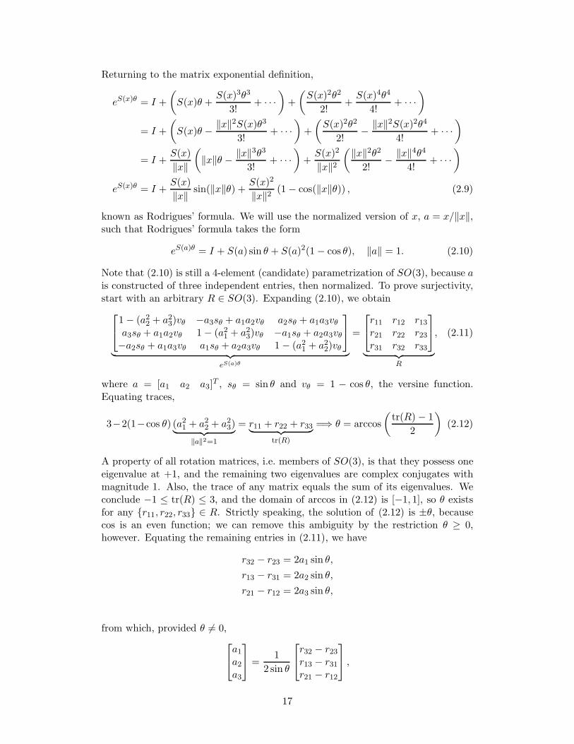
Returning to the matrix exponential definition,
eS(x)θ = I +
(S(x)θ +
S(x)3θ3
3!+ · · ·
)+
(S(x)2θ2
2!+S(x)4θ4
4!+ · · ·
)
= I +
(S(x)θ − ‖x‖2S(x)θ3
3!+ · · ·
)+
(S(x)2θ2
2!− ‖x‖2S(x)2θ4
4!+ · · ·
)
= I +S(x)
‖x‖
(‖x‖θ − ‖x‖3θ3
3!+ · · ·
)+S(x)2
‖x‖2(‖x‖2θ2
2!− ‖x‖4θ4
4!+ · · ·
)
eS(x)θ = I +S(x)
‖x‖ sin(‖x‖θ) + S(x)2
‖x‖2 (1− cos(‖x‖θ)) , (2.9)
known as Rodrigues’ formula. We will use the normalized version of x, a = x/‖x‖,such that Rodrigues’ formula takes the form
eS(a)θ = I + S(a) sin θ + S(a)2(1− cos θ), ‖a‖ = 1. (2.10)
Note that (2.10) is still a 4-element (candidate) parametrization of SO(3), because ais constructed of three independent entries, then normalized. To prove surjectivity,start with an arbitrary R ∈ SO(3). Expanding (2.10), we obtain
1− (a22 + a23)vθ −a3sθ + a1a2vθ a2sθ + a1a3vθa3sθ + a1a2vθ 1− (a21 + a23)vθ −a1sθ + a2a3vθ−a2sθ + a1a3vθ a1sθ + a2a3vθ 1− (a21 + a22)vθ
︸ ︷︷ ︸eS(a)θ
=
r11 r12 r13r21 r22 r23r31 r32 r33
︸ ︷︷ ︸R
, (2.11)
where a = [a1 a2 a3]T , sθ = sin θ and vθ = 1 − cos θ, the versine function.
Equating traces,
3−2(1−cos θ) (a21 + a22 + a23)︸ ︷︷ ︸‖a‖2=1
= r11 + r22 + r33︸ ︷︷ ︸tr(R)
=⇒ θ = arccos
(tr(R)− 1
2
)(2.12)
A property of all rotation matrices, i.e. members of SO(3), is that they possess oneeigenvalue at +1, and the remaining two eigenvalues are complex conjugates withmagnitude 1. Also, the trace of any matrix equals the sum of its eigenvalues. Weconclude −1 ≤ tr(R) ≤ 3, and the domain of arccos in (2.12) is [−1, 1], so θ existsfor any r11, r22, r33 ∈ R. Strictly speaking, the solution of (2.12) is ±θ, becausecos is an even function; we can remove this ambiguity by the restriction θ ≥ 0,however. Equating the remaining entries in (2.11), we have
r32 − r23 = 2a1 sin θ,
r13 − r31 = 2a2 sin θ,
r21 − r12 = 2a3 sin θ,
from which, provided θ 6= 0,
a1a2a3
=
1
2 sin θ
r32 − r23r13 − r31r21 − r12
,
17

which proves the existence of a for any r12, r13, r21, r23, r31, r32 entries of R pro-vided θ 6= 0. Consider the θ = 0 case, which only occurs when tr(R) = 3 in (2.12).Since R has orthonormal columns, this is only possible for R = I. Returning to(2.11), we have
1− (a22 + a23)0 −a30 + a1a20 a20 + a1a30a30 + a1a20 1− (a21 + a23)0 −a10 + a2a30−a20 + a1a30 a10 + a2a30 1− (a21 + a22)0
=
1 0 00 1 00 0 1
,
which is obviously satisfied for any a, meaning R = I is in the range of eS(a)θ aswell. This completes the proof of surjectivity, and we have shown that eS(a)θ fullyparameterizes SO(3). Comparing this result with Euler’s Rotation Theorem, wesee that a physically represents the (normalized) axis of rotation and θ the anglethrough which the object is rotated. θ = 0 is the no-rotation case, in which case anyrotation axis a can be used in the exponential. From the proof, we see that a given Rconfiguration yields a unique a, θ pair (as long as θ > 0 is assumed, otherwise bothθ, a and −θ,−a are solutions), except at R = I, where an infinity of solutionsexist. This effect is known as a singularity of the parametrization, because it destroysthe continuous nature of the inverse problem (finding the set of parameters givenan orientation R). Singularities are also discussed in Section 2.6.
Consider the matrix exponential eS(x), where x ∈ R3 is not necessarily of unit
length. Clearly,eS(x) = eS(x/‖x‖) ‖x‖.
By rotating x (changing its entries while keeping ‖x‖ constant), it is possible forx/‖x‖ to span the entire set a ∈ R
3, ‖a‖ = 1; this is true for any choice of ‖x‖ ∈ R.In this way, eS(x) can be made equal to eS(a)θ, ‖a‖ = 1, θ ∈ R, which was shownto be surjective onto SO(3). Since x ∈ R
3, we conclude it is possible to surjectivelyparameterize SO(3) with only three parameters.
2.6 Euler Angles Parametrization
Having shown that R ∈ SO(3) can be parameterized using only three numbers, wenow develop a concrete case, Euler angles. We will compose three rotations, eachdescribed by one angle, to produce the final orientation R. The composition ofrotations was discussed in Section 2.1.
n1
n2
n3
b1
b2
b3γ1
n1
n2
n3
b1
b2
b3
γ2n1
n2
n3
b1b2
b3
γ3
Figure 2.4: Elementary rotations about n1, n2 and n3
We first derive the rotation matrices about the three basis axes, illustrated inFigure 2.4. Note that unlike Section 2.1, all three rotations are made with respect
18

to the same frame N instead of using the previous frame as the “datum”. This willbe reflected in the physical interpretation of Euler Angles below — however, thecomposition of rotations still holds because R measures only the rotation betweentwo frames, so composing three rotations relative to N is mathematically identicalto the case in Section 2.1. Using the definition of R from Section 2.1,
RBN =
b1 · n1 b2 · n1 b3 · n1b1 · n2 b2 · n2 b3 · n2b1 · n3 b2 · n3 b3 · n3
,
we work out the rotations about n1, n2 and n3 as
R1(γ1) =
1 0 00 cos γ1 cos(π/2 + γ1)0 cos(π/2 − γ1) cos γ1
=
1 0 00 cos γ1 − sin γ10 sin γ1 cos γ1
, (2.13a)
R2(γ2) =
cos γ2 0 cos(π/2 − γ2)0 1 0
cos(π/2 + γ2) 0 cos γ2
=
cos γ2 0 sin γ20 1 0
− sin γ2 0 cos γ2
, (2.13b)
R3(γ3) =
cos γ3 cos(π/2 + γ3) 0cos(π/2− γ3) cos γ3 0
0 0 1
=
cos γ3 − sin γ3 0sin γ3 cos γ3 00 0 1
. (2.13c)
It’s easy to directly verify that each matrix in (2.13) belongs to SO(3).As seen in Section 2.1 composing rotations corresponds to matrix multiplication,
hence the order is not commutative. Any three-part sequence is valid providedadjacent rotations are not made about the same axis, which gives 3 × 2 × 2 = 12possible parameterizations. We choose to use the so-called roll-pitch-yaw sequence,the most widely used in aerospace literature. This sequence is defined by
RBN = R3(ψ)R2(θ)R1(φ), (2.14)
where roll φ, pitch θ and yaw ψ are defined as rotations about the x, y and z axes,respectively. Substituting (2.13) into (2.14) and performing matrix multiplicationgives
RBN =
cθcψ sφsθcψ − cφsψ cφsθcψ + sφsψcθsψ sφsθsψ + cφcψ cφsθsψ − sφcψ−sθ sφcθ cφcθ
, (2.15)
where cφ = cosφ, etc. Since Rk ∈ SO(3) we know RBN ∈ SO(3). As will be shownbelow, roll-pitch-yaw is surjective but not injective onto SO(3).
Physically, the composition (2.14) represents an ordered sequence of rotations ofthe helicopter body frame with respect to the ground. As seen in Figure 2.4, R1,R2 and R3 represent rotations with respect to the N frame, so (2.14) correspondsto the following rotation sequence, starting from a level flight configuration (framesN and B aligned, R = I):
1. Rotate the helicopter about n1 by φ (roll)
2. Rotate about n2 by θ (pitch)
3. Rotate about n3 by ψ (yaw).
19

It is also possible to interpret the angles φ, θ, ψ from a body-frame point of view.Starting from R = I, the rotations are made with respect to b1, b2 and b3, requiringthe transpose version of (2.13) because RBN = (RNB )
T as shown in Section 2.1. Notethe base frame B gets rotated at each step, but once again the mathematical formof composing rotations remains the same. For reasons that will become clear soonthe rotation sequence is done “backwards” from the one above:
1. Rotate the helicopter about b3 by ψ (yaw)
2. Rotate about b2 by θ (pitch)
3. Rotate about b1 by φ (roll)
This sequence of rotations composes to
RNB = R1(φ)TR2(θ)
TR3(ψ)T
and transposing both sides gives
RBN = R3(ψ)R2(θ)R1(φ),
which is identical to (2.14) above. In this sense, roll-pitch-yaw represents both theground-fixed rotation sequence
Roll φ around n1 =⇒ Pitch θ around n2 =⇒ Yaw ψ around n3,
and the body-fixed rotation sequence
Yaw ψ around b3 =⇒ Pitch θ around b2 =⇒ Roll φ around b1.
Consider the numerical example φ = −π/2, θ = π/2, ψ = π. This sequence canbe executed in either the ground-fixed or body-fixed order, giving the same finalconfiguration as illustrated in Figure 2.5. Remark that the body frame axes bk arerotated at each step.
Consider the inverse problem of calculating the sequence φ, θ, ψ given an ori-entation R. Starting from (2.15),
R =
cθcψ sφsθcψ − cφsψ cφsθcψ + sφsψcθsψ sφsθsψ + cφcψ cφsθsψ − sφcψ−sθ sφcθ cφcθ
=
r11 r12 r13r21 r22 r23r31 r32 r33
. (2.16)
By inspection, θ = − arcsin r31. Since R ∈ SO(3) the matrices (2.16) are orthonor-mal. It follows that |r31| ≤ 1 and so −π/2 ≤ θ ≤ π/2. Consider first the case|θ| < π/2, from which cθ 6= 0 and thus
tanφ =r32r33
=⇒ φ = atan2(r32, r33)
tanψ =r21r11
=⇒ ψ = atan2(r21, r11)
where atan2 is the “smart” arctan function which assigns the correct quadrantand handles the case of division by zero. Since arcsin and arctan are injectivefunctions and the entire range of R is in their domain, roll-pitch-yaw is a bijective
20
n1
n2n3
b1b1
b1
b1b1
b1
b1
b2
b2b2
b2b2
b2
b2b3
b3
b3
b3
b3b3
b3
n1, φ
n2, θ n3, ψ
b3, ψ
b2, θ b1, φ
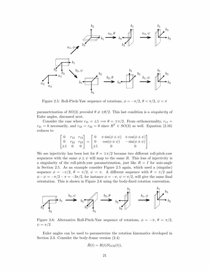
Figure 2.5: Roll-Pitch-Yaw sequence of rotations, φ = −π/2, θ = π/2, ψ = π
parametrization of SO(3) provided θ 6= ±θ/2. This last condition is a singularity ofEuler angles, discussed next.
Consider the case where r31 = ±1 =⇒ θ = ∓π/2. From orthonormality, r11 =r21 = 0 necessarily, and r33 = r32 = 0 since RT ∈ SO(3) as well. Equation (2.16)reduces to
0 r12 r130 r22 r23±1 0 0
=
0 ∓ sin(φ± ψ) ∓ cos(φ± ψ)0 cos(φ± ψ) − sin(φ± ψ)±1 0 0
.
We see injectivity has been lost for θ = ∓π/2 because two different roll-pitch-yawsequences with the same φ ± ψ will map to the same R. This loss of injectivity isa singularity of the roll-pitch-yaw parametrization, just like R = I for axis-anglein Section 2.5. As an example consider Figure 2.5 again, which used a (singular)sequence φ = −π/2, θ = π/2, ψ = π. A different sequence with θ = π/2 andφ−ψ = −π/2− π = −3π/2, for instance φ = −π, ψ = π/2, will give the same finalorientation. This is shown in Figure 2.6 using the body-fixed rotation convention.
b1
b1 b1
b1 b2 b2 b2
b2b3
b3
b3
b3
b3, ψ b2, θ b1, φ
Figure 2.6: Alternative Roll-Pitch-Yaw sequence of rotations, φ = −π, θ = π/2,ψ = π/2
Euler angles can be used to parameterize the rotation kinematics developed inSection 2.3. Consider the body-frame version (2.4)
R(t) = R(t)S(ωB(t)),
21

We use R from (2.15), compute R and solve the above for φ, θ, ψ. Since the Rexpression is quite long, we first group terms on the left side then perform the matrixmultiplication in e.g. Mathematica:
RT R = S(ωB)
0 sφθ − cφcθψ cφθ + sφcθψ
−sφθ + cφcθψ 0 −φ+ sθψ
−cφθ − sφcθψ φ− sθψ 0
=
0 −ωB,3 ωB,2ωB,3 0 −ωB,1−ωB,2 ωB,1 0
.
Isolating ωB,
ωB,1ωB,2ωB,3
=
φ− sθψ
cφθ + sφcθψ
−sφθ + cφcθψ
=
1 0 −sθ0 cφ sφcθ0 −sφ cφcθ
φ
θ
ψ
Inverting, we obtain
φ
θ
ψ
=
1 sinφ tan θ cosφ tan θ0 cosφ − sinφ0 sinφ sec θ cosφ sec θ
ωB,1ωB,2ωB,3
,
or equivalentlyφ = ωB,1 + sinφ tan θ ωB,2 + cosφ tan θ ωB,3
θ = cosφωB,2 − sinφωB,3
ψ = sinφ sec θ ωB,2 + cosφ sec θ ωB,3
(2.17)
Equations (2.17) are the dynamics of the roll-pitch-yaw Euler angle parametriza-tion. Remark the dynamics involve trig functions and become undefined at theparametrization singularity θ = ±π/2, making them a poor choice for numericalimplementation.
As mentioned previously, roll-pitch-yaw is just one of twelve possible Euler Angleparameterizations. It can be verified that all exhibit singularities, and in moregeneral terms it can be shown that any three-element parametrization of SO(3) willpossess singularities [125]. A practical solution is avoiding configurations which aresingular, e.g. never pitching the helicopter straight up or down. A more elegantsolution is to use a parametrization with > 3 elements which does not containsingularities, specifically unit quaternions discussed in the next section.
2.7 Quaternions
Quaternions were first introduced by Hamilton as a generalization of complex num-bers. Just as complex numbers on the unit circle can represent planar rotations viaeiθ, unit-length quaternions can represent three-dimensional rotations.
A quaternion r ∈ H is defined as
r = r0 + r1i+ r2j + r3k
where (r0, r1, r2, r3) ∈ R4 and H is a four-dimensional vector space over the reals
with basis vectors 1, i, j,k ∈ H. A quaternion can be written as r = (r0, ~r)
22
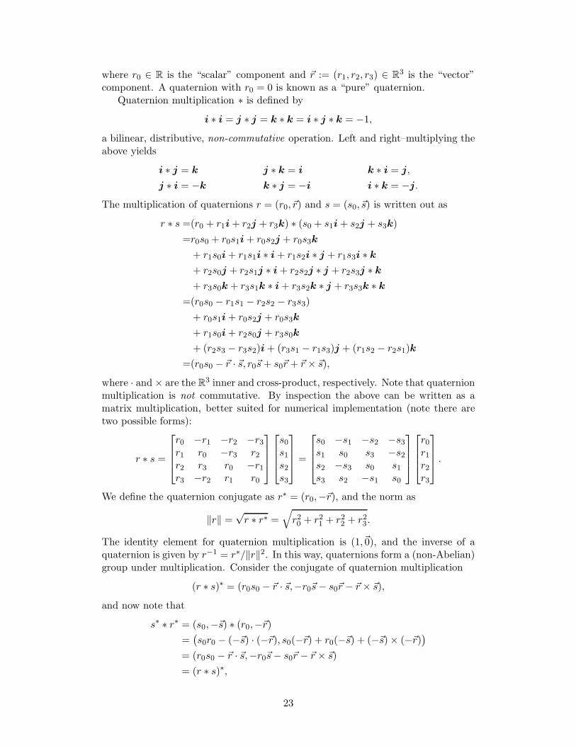
where r0 ∈ R is the “scalar” component and ~r := (r1, r2, r3) ∈ R3 is the “vector”
component. A quaternion with r0 = 0 is known as a “pure” quaternion.Quaternion multiplication ∗ is defined by
i ∗ i = j ∗ j = k ∗ k = i ∗ j ∗ k = −1,
a bilinear, distributive, non-commutative operation. Left and right–multiplying theabove yields
i ∗ j = k j ∗ k = i k ∗ i = j,
j ∗ i = −k k ∗ j = −i i ∗ k = −j.
The multiplication of quaternions r = (r0, ~r) and s = (s0, ~s) is written out as
r ∗ s =(r0 + r1i+ r2j + r3k) ∗ (s0 + s1i+ s2j + s3k)
=r0s0 + r0s1i+ r0s2j + r0s3k
+ r1s0i+ r1s1i ∗ i+ r1s2i ∗ j + r1s3i ∗ k+ r2s0j + r2s1j ∗ i+ r2s2j ∗ j + r2s3j ∗ k+ r3s0k + r3s1k ∗ i+ r3s2k ∗ j + r3s3k ∗ k
=(r0s0 − r1s1 − r2s2 − r3s3)
+ r0s1i+ r0s2j + r0s3k
+ r1s0i+ r2s0j + r3s0k
+ (r2s3 − r3s2)i+ (r3s1 − r1s3)j + (r1s2 − r2s1)k
=(r0s0 − ~r · ~s, r0~s+ s0~r + ~r × ~s),
where · and × are the R3 inner and cross-product, respectively. Note that quaternionmultiplication is not commutative. By inspection the above can be written as amatrix multiplication, better suited for numerical implementation (note there aretwo possible forms):
r ∗ s =
r0 −r1 −r2 −r3r1 r0 −r3 r2r2 r3 r0 −r1r3 −r2 r1 r0
s0s1s2s3
=
s0 −s1 −s2 −s3s1 s0 s3 −s2s2 −s3 s0 s1s3 s2 −s1 s0
r0r1r2r3
.
We define the quaternion conjugate as r∗ = (r0,−~r), and the norm as
‖r‖ =√r ∗ r∗ =
√r20 + r21 + r22 + r23.
The identity element for quaternion multiplication is (1,~0), and the inverse of aquaternion is given by r−1 = r∗/‖r‖2. In this way, quaternions form a (non-Abelian)group under multiplication. Consider the conjugate of quaternion multiplication
(r ∗ s)∗ = (r0s0 − ~r · ~s,−r0~s− s0~r − ~r × ~s),
and now note that
s∗ ∗ r∗ = (s0,−~s) ∗ (r0,−~r)=(s0r0 − (−~s) · (−~r), s0(−~r) + r0(−~s) + (−~s)× (−~r)
)
= (r0s0 − ~r · ~s,−r0~s− s0~r − ~r × ~s)
= (r ∗ s)∗,
23

analogous to matrix multiplication; this property will be used shortly.In Section 2.5, we have shown that R ∈ SO(3) can be surjectively parameterized
by a rotation axis a, ‖a‖ = 1 and angle θ via the matrix exponential. Define theassociated quaternion
q = (cos(θ/2), a sin(θ/2)). (2.18)
Remark that ‖q‖ = 1 by construction. We now show that (2.18) is also surjectiveonto unit quaternions
q = (q0, ~q), q20 + ‖~q‖2 = 1.
For the scalar part,cos(θ/2) = q0 =⇒ θ = 2arccos q0,
and since |q0| ≤ 1 for a unit quaternion, θ can always be found. For the vector part,consider first the case θ 6= 0:
a sin(θ/2) = ~q =⇒ a =1√
1− q20
q1q2q3
=
~q
‖~q‖ ,
i.e. a unit rotation axis a can be found for any values of ~q. Now consider the caseθ = 0:
θ = 0 =⇒ q0 = 1 =⇒ ~q = ~0,
and the axis isa sin 0 = ~0 =⇒ a ∈ R
3 =⇒ a = ~0;
i.e. we have chosen a = ~0 when θ = 0. Note in this case, ‖a‖ 6= 1 in Equation (2.18);however, q = (1,~0), still a unit quaternion. We conclude that (2.18) is a surjectiveparametrization of unit quaternions.
We now relate unit quaternions q written as (2.18) to R ∈ SO(3). For the caseθ 6= 0, ‖a‖ = 1 and we use Rodrigues’ formula (2.10):
R = I + S
(~q√
1− q20
)sin(2 arccos q0) + S
(~q√
1− q20
)2
(1− cos(2 arccos q0))
= I + S(~q)2q0√
1− q20√1− q20
+ S(~q)22(1− q20)
1− q20
=
1 0 00 1 00 0 1
+ 2q0
0 −q3 q2q3 0 −q1−q2 q1 0
+ 2
−q22 − q23 q1q2 q1q3q1q2 −q21 − q23 q2q3q1q3 q2q3 −q21 − q22
=
1− 2(q22 + q23) 2q1q2 − 2q0q3 2q1q3 + 2q0q22q1q2 + 2q0q3 1− 2(q21 + q23) 2q2q3 − 2q0q12q1q3 − 2q0q2 2q2q3 + 2q0q1 1− 2(q21 + q22)
.
For θ = 0, q = (1,~0), which gives R = I above, which is consistent because θ = 0denotes the no-rotation case. We conclude the matrix above, equivalently writtenas
R =
q20 + q21 − q22 − q23 2(q1q2 − q0q3) 2(q1q3 + q0q2)2(q1q2 + q0q3) q20 − q21 + q22 − q23 2(q2q3 − q0q1)2(q1q3 − q0q2) 2(q2q3 + q0q1) q20 − q21 − q22 + q23
, (2.19)
24

is the rotation matrix corresponding to the unit quaternion q. An immediate benefitof quaternion parametrization is that (2.19) does not use trig functions, as comparedto e.g. roll-pitch-yaw in (2.15).
Using parametrization (2.19), we can investigate the injectivity of q onto SO(3).As with Euler angles, begin by equating (2.19) to an arbitrary R ∈ SO(3),
q20 + q21 − q22 − q23 2(q1q2 − q0q3) 2(q1q3 + q0q2)2(q1q2 + q0q3) q20 − q21 + q22 − q23 2(q2q3 − q0q1)2(q1q3 − q0q2) 2(q2q3 + q0q1) q20 − q21 − q22 + q23
=
r11 r12 r13r21 r22 r23r31 r32 r33
.
(2.20)Equating traces, and using the fact that ‖q‖ = 1 =⇒ q20 + q21 + q22 + q23 = 1,
3q20 − (q21 + q22 + q23) = r11 + r22 + r33
4q20 − 1 = r11 + r22 + r33
q0 = ±1
2
√1 + r11 + r22 + r33.
As shown in Section 2.5, −1 ≤ tr(R) ≤ 3, so q0 ∈ R, |q0| ≤ 1 as expected. Also notethere are two possible solutions to q0 — this will be discussed below. From (2.20)we also have
4q0q1 = r32 − r23
4q0q2 = r13 − r31
4q0q3 = r21 − r12,
so
q1 =r32 − r23
4q0, q2 =
r13 − r314q0
, q3 =r21 − r12
4q0.
Since the q0 sign choice is arbitrary, it follows that both q and −q map to the sameR, i.e. unit quaternions provide a two-to-one covering of SO(3). From (2.18) thisis equivalent to saying (θ, a) and (−θ,−a) produce the same rotation. This issueis easily resolved by always picking the q0 ≥ 0 value when converting R to q. Theother ambiguity is the q0 = 0 case, which occurs if θ = ±π in (2.18). We investigatethe limit
limq0→0
q1 = limq0→0
r32 − r234q0
.
Using (2.19), this can be rewritten as
limq0→0
2q2q3 + 2q0q1 − 2q2q3 + 2q0q14q0
= limq0→0
q0q1q0
,
and by using l’Hopital’s rule,limq0→0
q1 = q1,
i.e. a (unique) limit exists. The analogous result holds for q2 and q3, which completesthe proof that quaternions form a two-to-one covering of SO(3).
Although we have proven the limit to exist, numerical problems will appear asq0 → 0 in the formulas above. To resolve this issue, we return to Equation (2.20)
25

and arrange the diagonal entries as one of:
B = r11 − r22 − r33 = 3q21 − (q20 + q22 + q23)
C = −r11 + r22 − r33 = 3q22 − (q20 + q21 + q23)
D = −r11 − r22 + r33 = 3q23 − (q20 + q21 + q22),
which result in
q1 =±√1 + B2
, q2 =±√1 + C2
, q3 =±√1 +D2
,
respectively. Clearly if A = r11+r22+r33 = 0, then B, C,D 6= 0 and one of the aboveqk solutions can be used to find the remaining three entries of q. Since qk will beused in the denominator of the remaining entries, we use “option” maxA,B, C,Dto reduce numerical problems. The conversion formulas for each option are providedbelow:
A :
q0 =
√1 +A2
q1 =r32 − r23
2√1 +A
q2 =r13 − r31
2√1 +A
q3 =r21 − r12
2√1 +A
B :
q0 =r32 − r23
2√1 + B
q1 =
√1 + B2
q2 =r12 + r21
2√1 + B
q3 =r13 + r31
2√1 + B
C :
q0 =r13 − r31
2√1 + C
q1 =r12 + r21
2√1 + C
q2 =
√1 + C2
q3 =r23 + r32
2√1 + C
D :
q0 =r21 − r12
2√1 +D
q1 =r13 + r31
2√1 +D
q2 =r23 + r32
2√1 +D
q3 =
√1 +D2
We develop two useful properties of unit quaternions. Consider a rotation matrixacting on a vector:
~v ′ = R~v, R ∈ SO(3);~v,~v ′ ∈ R3.
Let v = (0, ~v) and v′ = (0, ~v ′) be two pure non-unit quaternions. We will show thatfor the unit quaternion q parameterizing R above,
v′ = q ∗ v ∗ q−1 = q ∗ v ∗ q∗.
26

Using the angle-axis form (2.18) of q and assuming θ 6= 0 so that ‖a‖ = 1,
q ∗ v ∗ q∗
= (cθ/2, asθ/2) ∗ (0, ~v) ∗ (cθ/2,−asθ/2)=(cθ/2, asθ/2
)∗ (~v · asθ/2, ~vcθ/2 + (a× ~v)sθ/2
)
=(− a · (a× ~v)︸ ︷︷ ︸
0
s2θ/2, c2θ/2~v + 2cθ/2sθ/2(a× ~v) + s2θ/2a(~v · a) + s2θ/2a× (a× ~v)
)
=(0, (1 − s2θ/2)~v + sθ(a× ~v) + s2θ/2a(a · ~v) + s2θ/2a× (a× ~v)
)
=(0, ~v + s2θ/2
(a(a · ~v)− ~v (a · a)︸ ︷︷ ︸
‖a‖2=1
)
︸ ︷︷ ︸a×(a×~v)
+sθ(a× ~v) + s2θ/2a× (a× ~v))
=(0, ~v + 2s2θ/2a× (a× ~v) + sθ(a× ~v)
)
=(0, ~v + (1− cθ)S(a)(S(a)~v) + sθS(a)~v
)
=(0, (I + sθS(a) + (1− cθ)S(a)
2)~v)
=(0, eS(a)θ~v
)
=(0, R~v
)
= v′.
If θ = 0, q = (1,~0) = q∗, and v′ = v, which is correct since θ = 0 corresponds toR = I.
The above leads to another property of unit quaternions. Composing rotationsas in Section 2.1, assume we have
~v ′ = R1~v, ~v′′ = R2~v
′; ~v,~v ′, ~v ′′ ∈ R3, R1, R2 ∈ SO(3).
It follows that~v ′′ = R2R1~v.
Using pure quaternions, the above are equivalent to
v′ = q1 ∗ v ∗ q∗1 , v′′ = q2 ∗ v′ ∗ q∗2,
and by substitution,
v′′ = q2 ∗ q1 ∗ v ∗ q∗1 ∗ q∗2= (q2 ∗ q1) ∗ v ∗ (q2 ∗ q1)∗.
It follows that q2 ∗ q1 corresponds to the composed rotation R2R1 and so q2 ∗ q1 isa unit quaternion. This means that unit quaternions form a subgroup of H whosegroup operation ∗ composes rotations just as in the SO(3) group.
We will now use unit quaternions q to parameterize the rotation dynamics (2.4)R = RS(ωB) obtained in Section 2.3. Expanding RT R = S(ωB) using (2.19) weobtain four equations:
2
q0q0 + q1q1 + q2q2 + q3q3−q1q0 + q0q1 + q3q2 − q2q3−q2q0 − q3q1 + q0q2 + q1q3−q3q0 + q2q1 − q1q2 + q0q3
=
0ωB,1ωB,2ωB,3
,
27

equivalent to
q0 q1 q2 q3−q1 q0 q3 −q2−q2 −q3 q0 q1−q3 q2 −q1 q0
q0q1q2q3
=
1
2
0ωB,1ωB,2ωB,3
.
Inverting,
q0q1q2q3
=
1
2
q0 −q1 −q2 −q3q1 q0 −q3 q2q2 q3 q0 −q1q3 −q2 q1 q0
0ωB,1ωB,2ωB,3
,
the matrix form of the quaternion multiplication
q =1
2q ∗ (0, ~ωB) (2.21)
which can also be expressed as
q0q1q2q3
=
1
2
0 −ωB,1 −ωB,2 −ωB,3ωB,1 0 ωB,3 −ωB,2ωB,2 −ωB,3 0 ωB,1ωB,3 ωB,2 −ωB,1 0
q0q1q2q3
.
Similarly for (2.3) we have RRT = S(ωN ) and obtain
2
q0q0 + q1q1 + q2q2 + q3q3−q1q0 + q0q1 − q3q2 + q2q3−q2q0 + q3q1 + q0q2 − q1q3−q3q0 − q2q1 + q1q2 + q0q3
=
0ωN,1ωN,2ωN,3
q0 q1 q2 q3−q1 q0 −q3 q2−q2 q3 q0 −q1−q3 −q2 q1 q0
q0q1q2q3
=
1
2
0ωN,1ωN,2ωN,3
q0q1q2q3
=
1
2
q0 −q1 −q2 −q3q1 q0 q3 −q2q2 −q3 q0 q1q3 q2 −q1 q0
0ωN,1ωN,2ωN,3
=1
2
0 −ωN,1 −ωN,2 −ωN,3ωN,1 0 −ωN,3 ωN,2ωN,2 ωN,3 0 −ωN,1ωN,3 −ωN,2 ωN,1 0
q0q1q2q3
=⇒ q =1
2(0, ~ωN ) ∗ q (2.22)
2.8 Earth’s Magnetic Field
The Earth’s magnetic fieldm can be visualized by modeling the Earth as a magneticdipole, with magnetic field lines emanating vertically from the southern magnetic
28

Ω
m
Figure 2.7: Earth’s Magnetic Field
pole, running nearly parallel to the surface near the equator, and sinking verticallyinto the north magnetic pole as illustrated in Figure 2.7.
We distinguish between magnetic and geographic (“true”) north: the magneticnorth is defined as the geographic location where the magnetic field lines pointvertically down into the ground, while geographic north is defined by the location ofthe Earth’s rotation axis which also defines latitude 90 N. The magnetic north isnot fixed; for instance in 2010 it was located at 84.97 N, 132.35 W, drifting North-West at approximately 55 km/year. For this reason geographic north is always usedfor navigation, and the N frame’s n1 and n2 axes (c.f. Section 2.4) are defined aspointing respectively in geographic north and east directions. A hand-held compassmeasures the direction of magnetic north and its reading must be corrected by thedeclination angle λ between true and magnetic north at a given geographic location.In Edmonton λ > 0 indicates magnetic north is east relative to geographic north.
The SI unit for the magnetic field is the Tesla. A 1 T field is extremely strongso a more common unit is the Gauss where 1 T = 1 × 10⁴ G. The magnetic fieldvector m varies in magnitude and direction over the surface of the Earth, but canbe taken as constant for a given geographic location. The on-board IMU’s triaxialmagnetometer directly measures mB with a range of ±1.2 G and a resolution of0.2 mG on each axis. The reference magnetic field vector coordinates mN as wellas declination angle λ can be computed for a given location and date using theInternational Geomagnetic Reference Field (IGRF) [2] or World Magnetic Model(WMM) [98] models1. For instance the ERCHA flight field located at 5325′12” N,11323′58” W, alt = 712.2 m has the magnetic field value
mN =[0.1404 0.0386 0.5578
]TG, λ = 15.38
for September 1, 2011 using the IGRF model.
1An online calculator is available at http://www.ngdc.noaa.gov/geomagmodels/IGRFWMM.jsp.
29

2.8.1 Computing Yaw
During the navigation system’s initialization phase, the magnetometer is used tocalculate the yaw angle ψ of the helicopter w.r.t. the ground-fixed frame N , i.e. theangle of the longitudinal body-fixed axis b1 relative to geographic north direction n1.Together with roll φ and pitch θ angles, this is used to compute the initial attitudeR0 ∈ SO(3) of the vehicle.
The roll and pitch angles φ0 and θ0 of the helicopter during initialization cantypically be taken as zero since the helicopter starts out level on its landing skids.More generally these angles can be computed from the accelerometer: as discussedin Section 2.4 a stationary accelerometer outputs fB = −gB where gB = RT gN ,gN = [0 0 g]T and using (2.15),
fB,1fB,2fB,3
= −
cθcψ cθsψ −sθsφsθcψ − cφsψ sφsθsψ + cφcψ sφcθcφsθcψ + sφsψ cφsθsψ − sφcψ cφcθ
00g
=
sθ−sφcθ−cφcθ
g
such that
φ0 = arctan
(fB,2
fB,3
)and θ0 = arcsin
(fB,1g
)
are the initialization roll and pitch angles of the vehicle provided it is stationary.Remark the range of both arctan and arcsin is [−π/2, π/2] but the helicopter is notexpected to exceed this range during initialization.
Once initialization roll and pitch angles φ0, θ0 are available, the yaw angle ψ0 canbe computed from the magnetometer. Let mN := [Bx By Bz]
T be the (known)reference magnetic field in the navigation frame. We directly measure mB = RTmN
and from (2.14) and (2.13) we have
R1(φ)TR2(θ)
TR3(ψ)TmN = mB
R3(ψ)TmN = R2(θ)R1(φ)mB
cψ sψ 0−sψ cψ 00 0 1
BxByBz
=
cθ 0 sθ0 1 0
−sθ 0 cθ
1 0 00 cφ −sφ0 sφ cφ
mB,1
mB,2
mB,3
cψBx + sψBy−sψBx + cψBy
Bz
=
cθ sθsφ sθcφ0 cφ −sφ
−sθ cθsφ cθcφ
mB,1
mB,2
mB,3
The first two vector entries give
cψBx + sψBy = cθmB,1 + sφsθmB,2 + cφsθmB,3 = X−sψBx + cψBy = cφmB,2 − sφmB,3 = Y
Combining the above two equations leads to:
XBy − YBx = sψ(B2y +B2
x)
XBx + YBy = cψ(B2x +B2
y)
And so
tanψ =XBy − YBxXBx + YBy
=⇒ ψ = atan2(XBy − YBx,XBx + YBy),
30

or written out explicitly,
ψ = atan2
(By
[cθmB,1 + sφsθmB,2 + cφsθmB,3
]−Bx
[cφmB,2 − sφmB,3
],
Bx
[cθmB,1 + sφsθmB,2 + cφsθmB,3
]+By
[cφmB,2 − sφmB,3
]) (2.23)
Equation (2.23) provides a direct calculation for ψ, the yaw angle relative to truenorth. The disadvantage is the reliance onmN which is calculated from a theoreticalworld magnetic model and may be different in experiment due to warping of thelocal magnetic field by things such as ferromagnetic building materials or activemagnetic field sources such as power lines. We will revisit this point in Section 2.9.
An alternative approach to computing yaw is to consider a different ground-fixedframe whose first axis points in the direction of magnetic north. We denote this asthe magnetic frame M where m3 points vertically down just like in the navigationframe such that m2 points in the direction of magnetic east. The magnetic field mexpressed in M frame coordinates becomes mM := [BH 0 BV ]
T where BH andBV are the horizontal and vertical components of the magnetic field vector. Thevehicle’s yaw with respect to the magnetic north is known as the azimuth ψm. Theazimuth can be converted to navigation frame yaw ψ by ψ = ψm + λ where λ isthe local declination angle as discussed in Section 2.8. The advantage of using ψm
instead of ψ is that (2.23) simplifies considerably for mM :
ψm = atan2 (−cφmB,2 + sφmB,3, cθmB,1 + sφsθmB,2 + cφsθmB,3) , (2.24)
which does not employ the reference value of m. In addition to ψm we compute thevalue of the mM reference field using φ0, θ0 and mB : from (2.15),
mM =
BH0BV
=
∗ ∗ ∗∗ ∗ ∗
−sθ sφcθ cφcθ
mB,1
mB,2
mB,3
and soBV = − sin θ0 mB,1 + sinφ0 cos θ0 mB,2 + cosφ0 cos θ0 mB,3
BH =√m2B,1 + m2
B,2 + m2B,3 −B2
V
(2.25)
2.9 Magnetometer Calibration
The measurements made by a magnetometer sensor are affected by the surroundingenvironment (e.g. structural steel in buildings, power lines) as well as the vehicleitself (e.g. ferrous metal parts, engine magneto). Since the earth’s magnetic field isvery weak, uncompensated magnetometer readings cannot be trusted.
Field distortions present in the environment, e.g. inside a building, have anunknown spatially-varying nature and cannot be compensated for in practice. Forinstance, we have observed the measured magnetic field inside a lab shift by 90degrees just from moving the sensor close to the wall. For this reason all indoortesting is done in a prescribed section of the lab where magnetic interference has
31

been verified to be minimal, and the magnetic frame M is used as the ground-fixed frame to remove the need for a theoretical magnetic field value. Conversely,outdoor testing is conducted on a flying field situated far from buildings such thatthe reference magnetic field value mN is reliable and the navigation frame N canbe employed. This is important for GPS-aided navigation because the RNE matrixin (2.8) specifically requires the use of the N frame.
Field distortions caused by the vehicle body are fixed w.r.t. the magnetometersensor, and can be quantified and removed from subsequent sensor readings by acalibration procedure. The simplest approach is to collect a set of sensor readingsm while sequentially rotating the vehicle about the body-fixed axes b1, b2 andb3, each aligned with the magnetic East-West line. Since the theoretical magneticfield vector m is constant, the collected data points should trace out a 3-D spherecentered at zero with radius |m|. As shown in Figure 2.8 below, the actual sensorreadings will trace out a warped, offset sphere, whose center bm = mean(m) canbe computed and used to correct future measurements by m− bm. This method iscommonly known as Hard-Iron Calibration and is often found as a firmware featureon commercial magnetometers, including the IMU used in our helicopter UAV. Ithas the advantage of a simple calculation and not requiring knowledge of the localmagnetic field amplitude. Its disadvantage is the inability to compensate for fielddistortions which show up as a warping of the spherical shape.
A novel compensation approach is proposed in [54]. The magnetometer sensormodel is taken as
m =
ε1 0 0ε2 sin ρ1 ε2 cos ρ1 0
ε3 sin ρ2 cos ρ3 ε3 sin ρ3 ε3 cos ρ2 cos ρ3
m+
ζ1ζ2ζ3
= Kmm+ bm, (2.26)
where εk represent the sensor scaling errors, ρk the sensor misalignment angles,and ζk the sensor offsets of the individual magnetometer axes, 1 ≤ k ≤ 3. Physi-cally (2.26) models the following sources of magnetometer error: scale factor, mis-alignment, null shift (sensor bias), hard-iron and soft-iron errors [54]. Remark that(2.26) reduces to the Hard-Iron Calibration model by taking εk = 1 and ρk = 0resp. Km = I.
Equation (2.26) is inverted to m = K−1m (m−bm) and substituted into m2
1+m22+
m23 = |m|2 where |m| is known and constant, c.f. Section 2.8, resulting in
C1m21 + C2m1m2 + C3m1m3 + C4m
22 + C5m2m3 + C6m
23
+ C7m1 + C8m2 + C9m3 = C10 (2.27)
where the coefficients Cl are nonlinear functions of ε, ρ, ζ and |m|. Assume amagnetometer calibration data set m has been collected, consisting of N datapoints for which (2.27) holds. The system is rewritten as
m2
1,1 m1,1m2,1 · · · m3,1...
.... . .
...m2
1,N m1,Nm2,N · · · m3,N
C1/C10
...C9/C10
=
1...1
, (2.28)
from which a least-squares solution for the numerical values of C1/C10 . . . C9/C10 isperformed. This produces a system of nine nonlinear equations in nine unknowns ε,
32

ρ, ζ, which can be solved numerically. Using ε = 1, ρ = 0, ζ = 0 as initial guesses,the solution converges rapidly. The calibration constants are then substituted backinto (2.26), and future sensor readings are corrected as K−1
m (m− bm) := Acm+ bc,a linear mapping.
−1 −0.5 0 0.5 1−1
−0.5
0
0.5
1
m1 [G]
m2 [G
]
−1 −0.5 0 0.5 1−1
−0.5
0
0.5
1
m1 [G]
m3 [G
]
−1 −0.5 0 0.5 1−1
−0.5
0
0.5
1
m2 [G]
m3 [G
]
0 5000 100000.2
0.4
0.6
0.8
1
IMU sample
||m||
[G]
FullHI
Raw HI Full
Raw
HI
Full
Raw
Raw
HI
Full
Figure 2.8: Magnetometer Calibration, Engine Off: Raw Sensor Readings, Hard-Iron Compensated, Fully Compensated
The data collected during engine-off calibration is plotted alongside its hard-iron and fully-compensated versions in Figure 2.8. Observe the original data’s offsetcentre is corrected by both methods, but only the full compensation (2.26) correctsthe elliptical distortion. The magnitude plot in the bottom-right corner confirmsthe improvement in accuracy. The impact of magnetometer calibration on the ex-perimental performance of an aided inertial navigation system will be covered inSection 3.4.2.
Running the helicopter’s engine creates substantial distortions in the measuredmagnetic field. For this reason, a separate engine-on calibration data set is collectedand the calculations above are repeated. The two sets of constants are given inTable 2.1. The change in parameters is pronounced, confirming that the runningengine has a significant impact on the sensed magnetic field. This will be shownthrough flight experiments in Section 3.4.3.
33

Table 2.1: Magnetometer Calibration Constantsε ρ ζ
Engine Off1.00441.08841.1423
−3.292
−3.934
6.242
0.0795−0.19780.2412
Engine On1.03731.26581.3635
4.211
−6.862
−12.380
0.06160.01490.0020
34

Chapter 3
Extended Kalman Filter Design
for Aided Navigation
As mentioned in Section 1.2.1 the Extended Kalman Filter (EKF) is the conven-tional method of choice for aided navigation design. We apply this method to twoexamples used for our helicopter UAV project: an Attitude and Heading ReferenceSystem (AHRS) and a Magnetometer-plus-GPS Aided Inertial Navigation System(Aided INS). The resulting designs are implemented and validated in experimentand provide a foundation for the invariant observer design in Chapter 4.
3.1 Overview of EKF
The method of the Extended Kalman Filter is to linearize the system dynamicsaround a nominal trajectory and use the resulting model in a Kalman filter, anoptimal linear time-varying observer used to estimate the state of the linearized sys-tem from sensor and aiding measurement signals corrupted by noise. The resultingestimates are then added to the nominal trajectory to obtain state estimates for thenonlinear system. A nonlinear system with noise inputs is written as
x = f(x, u,w)
y = h(x, v)(3.1)
where x and y are the state and output (aiding measurements) vectors, u is theinput (sensors) vector, and w, v are process and measurement Gaussian white noisevectors with zero mean and known covariance. Let (x, u, 0, 0) represent a nominal(noise-free) trajectory of (3.1), i.e. one which satisfies
˙x = f(x, u, 0)
y = h(x, 0)(3.2)
where y is the nominal output. Linearizing (3.1) about the nominal trajectory weobtain
x = f(x, u, 0) +∂f
∂x
∣∣∣∣x,u,0
(x− x) +∂f
∂u
∣∣∣∣x,u,0
(u− u) +∂f
∂w
∣∣∣∣x,u,0
(w − 0)
y = h(x, 0) +∂h
∂x
∣∣∣∣x,0
(x− x) +∂h
∂v
∣∣∣∣x,0
(v − 0),
35

and after defining δx = x − x, δy = y − y and the Jacobian matrices F (t) =(∂f/∂x)(x, u), G(t) = (∂f/∂w)(x, u), H(t) = (∂h/∂x)(x) and L(t) = (∂h/∂v)(x),we obtain the LTV system
δx = F (t)δx +G(t)w
δy = H(t)δx + L(t)v(3.3)
The nominal trajectory x can be either computed ahead of time as x = x∗, a designknown as the Linearized Kalman Filter (LKF); or x can be taken as the estimatedstate of (3.1) itself, equivalent to re-linearizing the system about its latest estimate,which is known as the Extended Kalman Filter. We use the latter approach since themotions of the vehicle cannot be predicted a priori. The EKF is an ad-hoc designbecause the convergence properties of the observer depend on the trajectories ofthe nonlinear system and we cannot formally prove non-local stability. Neverthelessthe EKF works well in practice due to its inherent robustness to sensor noise andtolerance of aiding measurement drop-outs. We will revisit the issue of observerstability in Chapter 4.
3.2 EKF Design
3.2.1 Complementary Filter Topology
For Aided INS designs, the EKF is used inside a complementary filter topology [34,Chap. 10]: the nominal system dynamics (3.2) are numerically integrated usinghigh-rate, low-accuracy sensor signals u to produce the (roughly) estimated statex =: x− of the nonlinear system (3.1). Whenever a low-rate, high-accuracy aidingmeasurement is available, x− is used to obtain the linearized model (3.3), usedby the Kalman Filter together with u and y to estimate δx, which corrects thenonlinear system state as x− + δx = x+. The updated state x+ is output to theuser and becomes the IC for the next integration of (3.2). Conversely if an aidingmeasurement is not available at the current time, x− is output directly and used forthe next (3.2) integration.
The complementary filter setup is ideal for Aided INS applications because ofthe multirate nature of the on-board sensors: in our system, the IMU providesaccelerometer, rate gyro and magnetometer information at 100 Hz whereas GPSinformation is available at 10 Hz and is subject to service drop-outs due to environ-mental conditions. For the AHRS, all sensor signals are available at 100 Hz, howeverthe aiding rate may be set lower to conserve CPU cycles since the numerical inte-gration is computationally much less expensive than the Kalman update. This isparticularly useful for implementation on low-power embedded systems.
3.2.1.1 AHRS
The topology of the AHRS is shown in Figure 3.1. The task of the system is toestimate the attitude of the vehicle, measured by the rotation matrix R ∈ SO(3) ofthe body-fixed frame relative to the ground-fixed magnetic frame (c.f. Section 2.9).The name AHRS comes from aviation where “attitude” means the roll and pitchangles of the vehicle i.e. its attitude w.r.t the horizon while “heading” is its yaw angleto magnetic north [9, p. 3-22]. The design is a complementary filter consisting of
36

high-rate integration of a rate gyro signal ω from the IMU and low-rate correction ofthe resulting estimates using magnetometer and accelerometer aiding measurementsvia the Extended Kalman Filter.
GyroAHRS
Dynamics
ExtendedKalmanFilter
OutputEquations
Mag
Accel
−+
−+
ω x
δx
ym
ya
ym
ya
δym
δya
Figure 3.1: Topology of AHRS; signal rate inversely proportional to dot spacing
3.2.1.2 Aided INS
The Mag-plus-GPS aided INS topology is shown in Figure 3.2. The system providesestimates of the position, velocity and attitude of the vehicle relative to the ground-fixed navigation frame. The high-rate signals are the accelerometer f and rategyro ω measurements provided by the IMU. The low-rate aiding measurements areobtained from the on-board magnetometer and GPS receiver. Remark that unlikeFigure 3.1 the system’s EKF employs input (sensor) signals u in addition to aidingmeasurements y.
IMUNavigationDynamics
ExtendedKalmanFilter
OutputEquations
Mag
GPS
−+
−+
f , ω x
δx
ym
yp
ym
yp
δym
δyp
Figure 3.2: Topology of Aided INS; signal rate inversely proportional to dot spacing
37

Table 3.1: Identified Noise Parameters – Engine Off [75]
σf σω βf σbf βω σbω σm[m/s3/2] [rad/
√s] [1/s] [m/s2] [1/s] [rad/s] [G
√s]
0.0079 0.0017 1.89/178 0.0042 1.89/562 0.00029 0.000580.0074 0.0017 1.89/562 0.0020 1.89/562 0.00038 0.000510.0090 0.0021 1.89/562 0.0016 1.89/562 0.00032 0.00051
3.2.2 Sensor Models
The on-board IMU is equipped with a triaxial accelerometer, rate gyro and magne-tometer, respectively measuring specific force fB = pB−gB , angular velocity ωB andthe Earth’s magnetic fieldmB = RTmG at a rate of 100 Hz wheremG = mM or mN
is the magnetic field vector in the ground-fixed frame coordinates, taken as knownand constant as discussed in Section 2.8. The measured data exhibits significantbias and noise effects, which must be accounted for. The proposed sensor modelswith frame subscripts omitted are
f = f + bf + νf
ω = ω + bω + νω
m = Kmm+ bm + νm
(3.4)
where each ν represents a Gaussian white noise vector with zero mean and diagonalcovariance matrix entries σ2. The noise properties of the accelerometer and rate gyrosensors were analyzed using the method of Allan Variance [12] by [75, Chap. 4], whoproposed modeling both bias terms as b = b0 + bt where b0 is the constant turn-onbias to be computed during initialization, and bt is the time-varying part describedas a Gauss-Markov random process
bt = −βbt +√
2βνb
where 1/β is the time constant of the process and νb is a Gaussian white noise vectoras before.
The Km ∈ R3×3 and bm ∈ R
3 in (3.4) are constant terms used to model thewarping of the magnetic field, found by performing a calibration as described inSection 2.9. For later convenience the magnetometer signal is rewritten as
m = K−1m (m− bm)︸ ︷︷ ︸
ycm
−K−1m νm︸ ︷︷ ︸νcm
=⇒ ycm = m+ νcm,
where as in Section 2.9
ycm = Acm+ bc, Ac := K−1m , bc := −K−1
m bm
is the compensated magnetometer measurement, and νcm := Acνm is still a Gaussianwhite noise vector due to the linear transformation [123, p. 60], with covariance(σcm)
2 = E〈νcm(νcm)T 〉 = Acσ2m(Ac)
T . The identified noise parameters for the engine-off case are provided in Table 3.1.
A GPS receiver measures the position of the antenna mounted on the tail ofthe vehicle w.r.t. the ECEF frame origin raE where by Section 2.4 raE = roE +RNE p
aN
38

with roE , RNE constant terms computed during initialization. The GPS receiver
runs its own Kalman filter, which provides position measurements yp = ra + νpalong with their estimated standard deviations σp and diagnostic information at10 Hz. Using carrier-phase differential GPS the receiver is capable of providing upto 2 cm circular error probable precision, however atmospheric conditions may causeperiods of decreased accuracy or measurement drop-outs which will be addressed inSection 3.2.10.2.
The accelerometer measures the difference between the vehicle’s inertial accel-eration and gravity, known as the specific force f = a − g. The standard practicein AHRS design is to use the accelerometer as a tilt sensor by assuming a = 0,which holds if the body is stationary. This assumption also holds for a stationaryengine-on vehicle exhibiting vibrations due to E〈a〉 = 0. Clearly, this assumptionis violated under any vehicle manoeuvres. For reasons explained in Section 3.2.6.1,in the AHRS design we take the accelerometer bias model as bf = bf0 where bf0 isthe constant turn-on bias which is found during initialization. The accelerometeroutput measurement (for the AHRS case) is thus written as
f ≈ −g =⇒ f − bf0︸ ︷︷ ︸ya
−νf ≈ −g =⇒ ya ≈ −g + νf ,
where ≈ is used to emphasize the a = 0 assumption does not always hold.
3.2.3 Dynamics and Output Equations
3.2.3.1 AHRS
The AHRS is described using states R and bω measuring attitude and rate gyrobias, respectively. Employing the body-frame rotational kinematics (2.4) with sensormodels (3.4) the AHRS dynamics are
R = RS(ω − bω − νω)
bω = −βω(bω − bω0) +√
2βωνbω(3.5)
The measured outputs are written as functions of state
ycm = RTmM + νcm
ya = −RT gM + νf(3.6)
where mM , gM are respectively the magnetic and gravity field vectors in magneticframe coordinates. The nominal (noise-free) trajectory x dynamics are
˙R = RS(ω − bω)
˙bω = −βω(bω − bω0)
(3.7)
with corresponding outputym = RTmM
ya = −RTgM(3.8)
As discussed in Section 3.2.2, the ya model implicitly assumes zero vehicle acceler-ation, which may be violated. The rate gyro constant turn-on bias bω0 is computedduring initialization.
39

3.2.3.2 Aided INS
The IMU is assumed to be located sufficiently close to the vehicle’s centre of massto directly measure its acceleration. Using sensor models from Section 3.2.2 withnavigation dynamics (2.5) from Section 2.4 gives
pN = vN
vN = R(f − bf − νf ) + gN
R = RS(ω − bω − νω)
bf = −βf (bf − bf0) +√2βfνbf
bω = −βω(bω − bω0) +√
2βωνbω
(3.9)
The nominal dynamics of the system are the noise-free version of (3.9)
˙pN = vN
˙vN = R(f − bf ) + gN
˙R = RS(ω − bω)
˙bf = −βf (bf − bf0)
˙bω = −βω(bω − bω0)
(3.10)
As in the AHRS the constant turn-on bias terms bf0 and bω0 will be computedduring the system’s initialization.
The output (aiding) measurements of the system are the position of the tail-mounted GPS antenna reported in E frame coordinates and the compensated mag-netometer output in the B frame. From Section 3.2.2
yp = roE +RNE (pN +RlB) + νp
ycm = RTmN + νcm(3.11)
where roE is the position vector of the navigation frame origin w.r.t. the ECEF frameorigin, RNE is the rotation matrix between N and E, lB is the position vector of theGPS antenna w.r.t. the body frame origin, and mN is the reference magnetic field inthe navigation frame. The terms roE and RNE are computed during the initializationperiod, c.f. Section 2.4. The lever-arm term lB is measured directly from the vehicle’sgeometry. The value ofmN is available from a magnetic reference model as discussedin Section 2.8. The corresponding nominal output equations are
yp = roE +RNE
(pN + RlB
)
ym = RTmN
(3.12)
3.2.4 Numerical Integration
The AHRS and Aided INS nominal dynamics (3.7) and (3.10) in Section 3.2.3 arenumerically integrated at the IMU sampling rate of 100 Hz. As discussed in Sec-tion 3.2.1 the resulting estimated state x− is periodically updated using the high-precision, low-rate aiding measurements via the Extended Kalman Filter.
40

Instead of directly numerically integrating the equations using e.g. Runge-Kutta,we solve them analytically then apply numerical quadrature if required. For bωdynamics in (3.7) and bf , bω dynamics in (3.10) we left-multiply by the integratingfactor
e∫ t
t0βds
= eβ(t−t0),
then integrate the result between t = t0 and t = t1. This gives:
eβ(t−t0)˙b(t) + eβ(t−t0)βb(t) = eβ(t−t0)βb0
d
dt
(eβ(t−t0)b(t)
)= eβ(t−t0)βb0
∫ t1
t0
d
dt
(eβ(t−t0)b(t)
)dt =
∫ t1
t0
eβ(t−t0)βdtb0
eβ(t1−t0)b(t1)− eβ(t0−t0)b(t0) =(eβ(t1−t0) − eβ(t0−t0)
)b0
b(t1) = e−β(t1−t0)(b(t0)− b0
)+ b0
For R dynamics in (3.7), (3.10) we right-multiply by the integrating factor
e−
∫ t
t0S(ω(s))ds
where ω(t) := ω(t)− bω(t), then integrate the result between t = t0 and t = t1:
˙R(t)e
−∫ t
t0S(ω(s))ds − R(t)S(ω(s))e
−∫ t
t0S(ω(s))ds
= 0
d
dt
(R(t)e
−∫ t
t0S(ω(s))ds
)= 0
∫ t1
t0
d
dt
(R(t)e
−∫ t
t0S(ω(s))ds
)dt =
∫ t1
t0
0 dt
R(t1)e−
∫ t1t0S(ω(s))ds = R(t0)e
−∫ t0t0S(ω(s))ds
R(t1) = R(t0)e∫ t1t0S(ω(s))ds
where we used the matrix exponential properties d/dt(eAt) = AeAt = eAtA, e−At =(eAt)−1 and e03×3 = I. We evaluate the integral using the trapezoidal rule
∫ b
af(x)dx ≈ (b− a)
f(a) + f(b)
2
so that the update equation is
R(t1) = R(t0) exp
((t1 − t0)
2S[ω(t0)− bω(t0) + ω(t1)− bω(t1)
])
Alternatively, define ξ ∈ R3 as
ξ :=(t1 − t0)
2
[ω(t0)− bω(t0) + ω(t1)− bω(t1)
]≈∫ t1
t0
ω(s)ds
and use Rodrigues’ formula (2.9) from Section 2.5 to express the exponential of askew-symmetric matrix:
R(t1) = R(t0)eS(ξ) = R(t0)
(I +
S(ξ)
‖ξ‖ sin ‖ξ‖ + S(ξ)2
‖ξ‖2 (1− cos ‖ξ‖))
41

which is equivalent to the previous numerical update but does not require computinga matrix exponential.
The vN and pN dynamics in (3.10) are directly solved by integrating both sides.The trapezoidal rule then gives
vN (t1) = vN (t0) +(t1 − t0)
2
[R(t0)
(f(t0)− bf (t0)
)+ R(t1)
(f(t1)− bf (t1)
)+ 2gN
]
and
pN (t1) = pN (t0) +(t1 − t0)
2
[vN (t0) + vN (t1)
]
3.2.5 Linearized Error Dynamics
The EKF requires a linearized system model (3.3) with state δx = x − x for theerror between the true and nominal system trajectories. In order to handle the termsR−R we use the following standard approach [51, 59]: use the ground-frame rotationkinematics (2.3) R = S(ωN )R and define ωN =: dγ/dt where γ ∈ R
3 is a vectorwhich will be used to measure attitude error; remark γ is expressed in navigationframe coordinates. Multiplying the above by dt and taking the approximationsdR ≈ R− R, dγ ≈ γ − γ = δγ gives
R− R ≈ S(δγ)R
which is left-multiplied by RT and right-multiplied by RT , giving
RT −RT ≈ RTS(δγ)
Transposing both sides then gives
R−R ≈ −S(δγ)R or equivalently R ≈ R+ S(δγ)R (3.13)
where we used the fact that S is a skew-symmetric matrix. The term δγ will beused to represent the error between R and R; the remaining states will use thedefault δx = x− x definition. The reason for redefining the attitude error is that asmentioned in Section 2.5, the 9 entries of R ∈ SO(3) are not independent of eachother and so using R−R as the error state would lead to a singular covariance matrixP (c.f. Section 3.2.8) in the EKF which is numerically difficult to maintain [84,Sec. VIII].
The EKF is an observer which estimates the state δx of the linearized sys-tem (3.3) using sensor (input) signals u and aiding (output) measurements y. Theestimate δγ ⊂ δx is used to update R to R; however, using the approximation (3.13)for this purpose causes R to lose orthogonality, creating significant problems in thealgorithm unless the resulting matrix is numerically re-orthogonalized after eachupdate, typically using SVD [51, p. 469]. A more elegant solution is to use an at-titude update which preserves orthogonality [17, 59]: for (2.3) R = S(ωN )R theintegrating factor is
e−
∫ t
t0S(ωN (s))ds
42

which left-multiplies the rotational kinematics (in contrast to Section 3.2.3):
e−
∫ t
t0S(ωN (s))ds
R(t)− e−
∫ t
t0S(ωN (s))ds
S(ωN (t))R(t) = 0
d
dt
(e−
∫ t
t0S(ωN (s))ds
R(t))= 0
∫ t1
t0
d
dt
(e−
∫ t
t0S(ωN (s))ds
R(t))dt =
∫ t1
t0
0 dt
e−∫ t1t0S(ωN (s))dsR(t1) = e−
∫ t0t0S(ωN (s))dsR(t0)
R(t1) = e∫ t1t0S(ωN (s))dsR(t0)
Using ωN(s) = dγ/ds as before with R(t0) = R, R(t1) = R we have
R = e∫ t1t0S(dγ/ds)dsR = eS(γ−γ)R = eS(δγ)R (3.14)
an attitude update which preserves orthogonality:
RRT = eS(δγ)RRT e−S(δγ) = eS(δγ)(1−1) = I
where we have used the identities (eA)T = eAT
and eAt1eAt2 = eA(t1+t2). Equa-tion (3.14) is used with δγ from the EKF to correct the state R obtained fromnumerical integration of the nominal dynamics. The remaining states are correcteddirectly from the definition of δx as
x = x+ δx
We now work out the linearized error dynamics and outputs for the AHRS andAided INS dynamics in Sections 3.2.3.1 and 3.2.3.2, respectively. For attitude errorsR− R, starting from (3.13), we have
R− ˙R = S(δγ)R+ S(δγ)
˙R
RS(ω − bω − νω) = RS(ω − bω) + S(δγ)R
+ S(δγ)RS(ω − bω)(R+ S(δγ)R
)S(ω − bω − νω) =
(R+ S(δγ)R
)S(ω − bω) + S(δγ)R
(R+ S(δγ)R
)S(ω − (bω + δbω)− νω) =
(R+ S(δγ)R
)S(ω − bω) + S(δγ)R
(R+ S(δγ)R
)S(−δbω − νω) = S(δγ)R
RS(−δbω − νω) + S(δγ)RS(−δbω − νω)︸ ︷︷ ︸≈0
= S(δγ)R
S(−δbω − νω) = RTS(δγ)R = S(RT δγ)
−δbω − νω = RT δγ
δγ = −Rδbω − Rνω
43

where the neglected expression consists of quadratic (i.e. non-linear) terms. For biaserrors δb = b− b, we have
δb = b− ˙b
= −β(b− b0) +√
2βνb + β(b− b0)
= −β(b− b) +√
2βνb
δb = −βδb+√
2βνb
an exact expression since the bias dynamics model is linear, c.f. Section 3.2.2. ForAided INS, the velocity error δv = v − v dynamics are
δv = R(f − bf − νf ) + gN − R(f − bf )− gN
= R(f − bf − νf )−R(f − bf ) +R(f − bf )− R(f − bf )
= −Rδbf −Rνf + (R − R)(f − bf )
= −Rδbf − S(δγ)Rδbf︸ ︷︷ ︸≈0
−Rνf − S(δγ)Rνf︸ ︷︷ ︸≈0
+S(δγ)R(f − bf )
= −Rδbf − Rνf + δγ ×(R(f − bf )
)= −Rδbf − Rνf −
(R(f − bf )
)× δγ
δv = −S(R(f − bf )
)δγ − Rδbf − Rνf
and for position error δp = p− p the dynamics are
δp = v − v = δv
The magnetometer output error is
δym = ycm − ym
= RTmG + νcm − RTmG
= (R− R)TmG + νcm
=(S(δγ)R
)TmG + νcm
= −RTS(δγ)mG + νcm
= −RT (δγ ×mG) + νcm
= RT (mG × δγ) + νcm
δym = RTS(mG)δγ + νcm
wheremG = mM for AHRS andmG = mN for Aided INS. The AHRS accelerometeroutput error δya is obtained simply by replacing mG by −gM and νcm by νf in thelast line above:
δya = −RTS(gM )δγ + νf
For Aided INS the GPS output error δyp is
δyp = yp − yp
= roE +RNE (pN +R lB) + νp − roE −RNE (pN + R lB)
= RNE
(δp + S(δγ)R lB
)+ νp
= RNE δp−RNES(R lB)δγ + νp
44

In each case the linearized error dynamics form the continuous-time LTV system(c.f. Section 3.1)
δx = F (t)δx +G(t)w
δy = H(t)δx + v,(3.15)
where the entries of F (t), G(t) and H(t) are read off the expressions above. Theresulting linearized error dynamics are summarized in Sections 3.2.5.1 and 3.2.5.2.
3.2.5.1 AHRS
The error system (3.15) is[δγ
δbω
]=
[0 −R0 −βω
] [δγδbω
]+
[−R 00
√2βω
] [νωνbω
]
[δycmδya
]=
[RTS(mM ) 0
−RTS(gM ) 0
] [δγδbω
]+
[νcmνf
] (3.16)
and the process and measurement noise vectors w and v are characterized by the co-variance matrices Q = E〈wwT 〉 = diag(σ2ω, σ
2bω) and R = E〈vvT 〉 = diag((σcm)
2, σ2f ).
3.2.5.2 Aided INS
The error system (3.15) is
δpδvδγ
δbfδbω
=
0 I 0 0 0
0 0 −S(R(f − bf )) −R 0
0 0 0 0 −R0 0 0 −βf 00 0 0 0 −βω
δpδvδγδbfδbω
+
0 0 0 0
−R 0 0 0
0 −R 0 0
0 0√
2βf 00 0 0
√2βω
νfνωνbfνbω
[δypδym
]=
[RNE 0 −RNES(R lB) 0 0
0 0 RTS(mN ) 0 0
]
δpδvδγδbfδbω
+
[νpνcm
]
(3.17)
The process and measurement noise vectors w and v are characterized by thecovariance matrices Q = E〈wwT 〉 = diag(σ2f , σ
2ω, σ
2bf , σ
2bω) and R = E〈vvT 〉 =
diag(σ2p, (σ
cm)
2).
3.2.6 Observability Analysis
As mentioned in Section 3.2.5, the LTV systems (3.16), (3.17) are used to the designthe EKF, an observer which estimates the state δx from inputs u and outputs ywhere u represents sensor signals which enter the Jacobians F (t), G(t), H(t) and yrepresents aiding measurements. We first verify the observability of these systems.
45

3.2.6.1 AHRS
Following [40, Theorem 6.O12], for a LTV system with state dimension n we definethe observability matrix
O(t) =
N0(t)N1(t)
...Nn−1(t)
whereN0(t) = H(t)
Nm+1(t) = Nm(t)F (t) + (d/dt)Nm(t), m = 0, . . . , n− 2
where F (t) and H(t) are the state and output matrices. For system (3.16), n = 6and we would need to compute terms up to N5(t). We have
N0(t) = H(t) =
[RTS(mM ) 0
−RTS(gM ) 0
]
and by (3.7),˙R = RS(ω − bω) =⇒ ˙
RT = −S(ω − bω)RT . We now compute
N1(t) = N0(t)F (t) + N0(t)
=
[RTS(mM ) 0
−RTS(gM ) 0
] [0 −R0 −βω
]+
[−S(ω − bω)R
TS(mM ) 0
S(ω − bω)RTS(gM ) 0
]
=
[0 −RTS(mM )R
0 RTS(gM )R
]+
[−S(ω − bω)R
TS(mM ) 0
S(ω − bω)RTS(gM ) 0
]
=
[−S(ω − bω)R
TS(mM ) −RTS(mM )R
S(ω − bω)RTS(gM ) RTS(gM )R
]
The observability matrix O(t) has the structure
N0(t)N1(t)∗
=
RTS(mM ) 0
−RTS(gM ) 0
−S(ω − bω)RTS(mM ) −RTS(mM )R
S(ω − bω)RTS(gM ) RTS(gM )R
∗ ∗
Consider the left half of the N0(t) line, written as
[RTS(mM )
−RTS(gM )
]=
[RT 0
0 RT
] [S(mM )−S(gM )
]
Since R ∈ SO(3) is always invertible, we have
rank
[RTS(mM )
−RTS(gM )
]= rank
[S(mM )−S(gM )
]
46

The magnetic and gravity field vectors are respectively mM = [BH 0 BV ]T and
gM = [0 0 g]T and so the term above expands to
rank
[S(mM )−S(gM )
]= rank
0 −BV 0BV 0 −BH0 BH 00 g 0−g 0 00 0 0
= 3
Next, consider the right half of the N1(t) line, written as
[−RTS(mM )R
RTS(gM )R
]=
[RT 0
0 RT
] [−S(mM )R
S(gM )R
]=
[RT 0
0 RT
] [−S(mM )S(gM )
] [R]
and with R ∈ SO(3) always invertible, we have
rank
[−RTS(mM )R
RTS(gM )R
]= rank
[−S(mM)S(gM )
]= 3,
since the expanded form is just a sign change of the earlier term. Due to the lower-triangular form of the N0(t) and N1(t) lines in O(t), we know (e.g. [67, p. 25])
rank
[N0(t)N1(t)
]≥ 3 + 3 =⇒ rank
[N0(t)N1(t)
]= 6 =⇒ rankO(t) = 6,
i.e. the observability matrix O(t) is always full rank. The LTV system (3.16) rep-resenting the AHRS linearized error dynamics is therefore observable at any timet ∈ (−∞,∞), and so is said to be instantaneously observable [39, p. 187].
The AHRS system in Section 3.2.3.1 could be expanded by including accelerom-eter bias as a dynamic state, i.e. adding
bf = −βf (bf − bf0) +√
2βfνbf
to (3.5) and using ya = f − bf in place of the current ya = f − bf0. In this case theLTV error system (3.16) increases its dimension to 9 and an observability analysisreveals the system is not observable unless it is rotating [51, p. 369]. We chose toinclude the rate gyro bias bω rather than accelerometer bias bf as a state becausethe former is used to integrate the rotation kinematics, hence a detailed model ofbω is more important than bf for accuracy of the AHRS.
3.2.6.2 Aided INS
The original implementation of a navigation filter for our helicopter UAV [75] usedthe GPS position yp as the sole aiding measurement, which was found to provide re-liable yaw estimates for trajectory flying but not in hover. An observability analysisof the LTV system (3.17) using δyp as the only output reveals the δγ3 state is unob-servable unless the vehicle is manoeuvering [117], meaning ψ will remain uncorrectedand slowly diverge in hover. This can be shown intuitively as follows: the only coef-ficient of δγ in (3.17) is S(R(f − bf )) := S(fN ) where fN denotes the bias-corrected
47

accelerometer measurement expressed in the navigation frame. Expanding S(fN )via (2.2) we see the coefficients of δγ3 will vanish when fN,1 = fN,2 = 0, i.e. zerolateral acceleration. Thus, unless the vehicle is manoeuvering, δγ3 cannot be ob-servable; the δγ term in δyp cannot be distinguished from δp and does not alter thisbehaviour.
This effect can be eliminated by adding an aiding sensor which provides δγ3observability, e.g. a magnetometer. The output equation δym in (3.17) containsS(mN )δγ and gives non-zero δγ3 coefficients provided mN 6= [0 0 ±|m|]T , whichwould only occur at the magnetic north or south poles. A different source of δγ3information such as a two-antenna GPS receiver [135] could also be employed.
The triaxial magnetometer part of the output matrix in (3.17) generally providescorrection information for all three components of δγ, i.e. it provides updates for theroll and pitch axes in addition to the yaw axis. This is due to S(mN )δγ = mN × δγin (3.17) providing observability for the part of δγ which is not parallel to mN . Thisis why δγ3 becomes unobservable at the magnetic poles and why δγ1 and δγ2 areobservable from δym as long as the rotation axis is not parallel to mN . However insome situations the magnetometer should only be used to provide information aboutthe yaw error state δγ3 [50, p. 28]; this will be further discussed in Sections 3.4.2and 3.4.3.
The yaw-only aiding equation is obtained as follows: starting from y − y =RTmN + νcm − RTmN , assume that roll and pitch are perfectly estimated by thenavigation filter, i.e. φ = φ and θ = θ. By (2.14) we have
R− R = R3(ψ)R2(θ)R1(φ)−R3(ψ)R2(θ)R1(φ)
and from (3.13)R3(ψ) −R3(ψ) ≈ S([0, 0, δγ3 ]
T )R3(ψ)
Using these expressions, we obtain the yaw-only magnetometer output equation
δym = RTS(mN )[0, 0, δγ3]T + νcm, (3.18)
which clearly provides observability of only δγ3.
3.2.7 Discretization
Since the aiding measurements are sampled, we use the discrete-time formulationof the Kalman Filter, which requires a discretized version of the linearized errorsystem (3.15). The details of how the resulting model is used by the EKF algorithmwill be covered in Section 3.2.8.
Let tk, tk+1 denote successive sampling times with τ = tk+1 − tk and xk bethe state estimate at t = tk, then evaluate (3.15) at xk to obtain Fk = F (xk),Gk = G(xk), Hk = H(xk) which are assumed constant on t ∈ [tk, tk+1]. Theresulting LTI system is then solved as
δxk+1 = eFkτδxk +
∫ tk+1
tk
eFk(tk+1−t)Gkw(t)dt = Φkδxk + wk
δyk = Hkδxk + vk
48

where wk represents a white sequence whose covariance is given by
Qk = E⟨wkw
Tk
⟩
= E
⟨∫ tk+1
tk
eFk(tk+1−t)Gkw(t)dt
∫ tk+1
tk
wT (s)GTk eFTk(tk+1−s)ds
⟩
= E
⟨∫ tk+1
tk
∫ tk+1
tk
eFk(tk+1−t)Gkw(t)wT (s)GTk e
FTk(tk+1−s)dt ds
⟩
=
∫ tk+1
tk
∫ tk+1
tk
eFk(tk+1−t)Gk E⟨w(t)wT (s)
⟩︸ ︷︷ ︸
Qδ(s−t)
GTk dt eFTk(tk+1−s)ds
Qk =
∫ tk+1
tk
eFk(tk+1−s)GkQGTk e
FTk(tk+1−s)ds (3.19)
where we used the definition of continuous-time white noise [34, p. 92] as a stationaryrandom process with autocorrelation E〈ν(t)ν(t + s)〉 = σ2δ(s) where δ denotes theDirac delta function. The Qk term (3.19) can be numerically evaluated using thefollowing method adapted from [130]: form the matrix
M =
[A1 B1
0 A2
]
where A1, A2 and B1 are square matrices with the same dimensions. Due to itsupper block-triangular structure, the matrix exponential of M takes the form
eMt =
[C1(t) D1(t)0 C2(t)
]
Since (d/dt)eMt = MeMt and e0 = I, we obtain the set of matrix differentialequations
C1(t) = A1C1(t) C1(0) = I
C2(t) = A2C2(t) C2(0) = I
D1(t) = A1D1(t) +B1C2(t) D1(0) = 0
whose solution is
C1(t) = eA1t
C2(t) = eA2t
D1(t) =
∫ t
0eA1(t−s)B1e
A2sds
whereD1(t) is found using the integrating factor approach employed in Section 3.2.4.To evaluate (3.19), form the matrix
M =
[−Fk GkQG
Tk
0 F Tk
]
and recall τ = tk+1 − tk. Evaluating the matrix exponential eMτ then gives
eMτ =
[N1 N2
0 N3
]=
[e−Fkτ
∫ τ0 e
−Fk(τ−s)GkQGTk e
FTksds
0 eFTkτ
]
49

Using the change of variables s = tk+1 − t,
N2 = e−Fkτ
∫ τ
0eFksGkQG
Tk e
FTksds
=(eFkτ
)−1∫ tk+1
tk
eFk(tk+1−t)GkQGTk e
FTk(tk+1−t)dt
and referring to (3.19),Qk = (N3)
T N2
Remark that (N3)T = eFkτ = Φk, the transition matrix of the DT system.
The covariance of vk, the measurement noise white sequence, is found as follows:first consider a continuous-time signal f(t) with Fourier transform Fc(ω) and sampleit with a period of T . The discrete-time Fourier transform Fd(Ω) of the resultingsignal f [k] can be shown to be [82, p. 636]
Fd(Ω) =1
TFc
(Ω
T
)
where Fd(Ω) has a period of 2π; this relationship holds irrespective of whether f(t)is bandlimited or whether it is sampled above its Nyquist rate. A continuous-timewhite noise term ν is defined by its autocorrelation R(τ) = E 〈ν(t)ν(t+ τ)〉 = σ2δ(τ)or equivalently by its power spectral density function
Sc(ω) = Fc (R(τ)) =∫ ∞
−∞σ2δ(τ)e−jωτdτ = σ2
The sampled version of ν is the discrete-time white sequence v[k], defined by theautocorrelation Rd[κ] = E〈v[k]v[k + κ]〉 = σ2dδκ or equivalently the power spectraldensity function
Sd(Ω) = Fd (Rd[κ]) =κ=∞∑
κ=−∞
σ2dδκe−jΩκ = σ2d
By the above we have
Sd(Ω) =1
TSc
(Ω
T
)=σ2
T
and so the sampled version of ν possesses the discrete-time covariance σ2d = σ2/T .For the measurement white sequence vk, this means
Rk =
(1
τ
)R
In summary we have converted (3.15) into the discrete-time LTV system
δxk+1 = Φkδxk + wk E〈wkwTk 〉 = Qk
δyk = Hkδxk + vk E〈vkvTk 〉 = Rk(3.20)
where Φk, Hk, Qk and Rk are calculated as above using the current state xk = x(tk)and interval between aiding measurements τ = tk+1 − tk.
50

3.2.8 Kalman Filter
The Kalman Filter applies to linear, discrete-time systems of the form (3.20) wherewk, vk are white sequences with known covariances Qk, Rk, respectively. We alsoassume that
E⟨wkv
Tl
⟩= 0 ∀k, l
The reason for this assumption will become clear in the derivation below; physically,this means the process and measurement noise are uncorrelated with each other.This is a reasonable assumption as seen from (3.16) and (3.17) where the processw and measurement v noise vectors are composed from different sensors. Note theKalman Filter can be modified to allow wk and vk to be correlated, c.f. [34, Sec. 9.2].
Define the pre-update estimate of the linearized system state δxk as δx−k and theassociated estimation error as e−k = δxk−δx−k with covariance P−
k = E⟨(e−k )(e
−k )
T⟩.
The Kalman filter is the linear observer
δxk = δx−k +Kk(δyk −Hkδx−k ), (3.21)
where Kk is chosen to minimize the trace of Pk = E⟨(δxk − δxk)(δxk − δxk)
T⟩=
E⟨ek e
Tk
⟩, the post-update error covariance. This last condition is the cost function
to be minimized, representing the sum of the variances of the individual entries of ek,the estimation error vector. Substituting (3.21) into Pk and expanding via (3.20),
Pk = E⟨(δxk − δx−k −Kk(δyk −Hkδx
−k )) (δxk − δx−k −Kk(δyk −Hkδx
−k ))T⟩
= E⟨(e−k −Kk(Hke
−k + vk)
) (e−k −Kk(Hke
−k + vk)
)T⟩
Pk = (I −KkHk)P−k (I −KkHk)
T +KkRkKTk , (3.22)
where we took E⟨e−k vk
⟩= E
⟨e−k⟩E 〈vk〉 = 0 due to the assumption that vk and wk
are uncorrelated. Equation (3.22) gives Pk as a quadratic function of Kk. Using thematrix differentiation formulas d (tr(AB)) /dA = BT , d
(tr(ACAT )
)/dA = 2AC,
we compute d (trPk) /dKk and find its minima:
d (trPk)
dKk= −2(HkP
−k )T + 2Kk(HkP
−k H
Tk +Rk) = 0
=⇒ Kk = P−k H
Tk (HkP
−k H
Tk +Rk)
−1,
(3.23)
whereKk is the optimal observer gain in (3.21). Using this value, we update the esti-mate δx−k using (3.21) and find the post-update error covariance of δxk using (3.22).Finally, we propagate the post-update δxk in time using (3.20) as
δx−k+1 = Φkδxk (3.24)
and the covariance Pk as
P−k+1 = E
⟨(δxk+1 − δx−k+1)(δxk+1 − δx−k+1)
T⟩
= E⟨(Φk(δxk − δxk) + wk)(Φk(δxk − δxk) + wk)
T⟩
P−k+1 = ΦkPkΦ
Tk +Qk, (3.25)
where E 〈ekwk〉 = E 〈ek〉E 〈wk〉 = 0 because wk is the process noise during thepropagation interval
(δxk, δx
−k+1
]and hence uncorrelated with ek. The δx−k+1 and
P−k+1 terms are used on the next Kalman Filter pass as δx−k and P−
k , respectively,making it a recursive algorithm well-suited for computer implementation.
51

3.2.9 Extended Kalman Filter
As explained in Section 3.1, the Extended Kalman Filter re-linearizes the nonlinearsystem (3.1) about its latest nominal state x and output y. The standard KalmanFilter algorithm in Section 3.2.8 is thus modified as described below.
Whenever an aiding measurement is available, the latest nominal state and out-put are obtained from integration of (3.2) as x−k and y−k , respectively, where the su-perscript − is used to denote pre-correction quantities. The states of the linearizederror system (3.20) are then δxk = xk−x−k and δyk = yk−y−k , the estimated Kalmanstates are δxk = xk − x−k and δx−k = x−k − x−k = 0, and so the update step (3.21)simplifies to
xk = x−k +Kk
(yk − y−k
)(3.26)
where Kk is computed by (3.23) and Pk is updated by (3.22) as in the conventionalKalman Filter. After update (3.26) is performed, the updated state xk immediatelybecomes the linearization trajectory, so δxk = xk − xk and δxk = xk − xk = 0.This means the estimated state propagation (3.24) becomes trivial and is omitted.The covariance matrix propagation step (3.25) still requires Φk and Qk, which arecalculated by the method in Section 3.2.7 using the just-updated state xk.
An important point for implementation is that the aiding measurements may beaperiodic, and so the EKF should not propagate Pk forwards in time. Instead, afterperforming the update (3.26), we save a copy of the updated state estimate xk, theerror covariance Pk obtained from (3.22) and the current aiding time ta. The nexttime an aiding measurement is available and the EKF is entered, we use the savedstate as xk−1 to build Fk−1, Gk−1, compute τ = t − ta, calculate Φk−1, Qk−1 anduse these to propagate the saved Pk−1 to P−
k by (3.25). This works because thecalculation method for Φk and Qk in Section 3.2.7 is time-invariant and requiresonly the elapsed time τ .
In summary, the EKF algorithm consists of the following sequence of operations,executed whenever an external aiding measurement is available:
1. Propagate previous covariance matrix: P−k = Φk−1Pk−1Φ
Tk−1 +Qk−1
2. Compute Kalman gain: Kk = P−k H
Tk (HkP
−k H
Tk +Rk)
−1
3. Update estimate: x = x− +Kk(yk − y−k )
4. Compute covariance of updated estimate: Pk = (I−KkHk)P−k (I−KkHk)
T +KkRkK
Tk
Following the above, the terms x and Pk are retained. On the next EKF pass, thesaved x is used as xk−1 to build Fk−1, Gk−1 to calculate Φk−1, Qk−1, and the savedPk as Pk−1 in step 1 above. To initialize the (recursive) EKF algorithm, xk−1 isassigned as the vehicle’s initial state estimate x(0), computed during an initializationperiod discussed in Section 3.2.11. The Pk−1 is assigned as a zero matrix, whichresults in sub-optimal estimates for the first few EKF passes but is numerically saferthan over-estimating the entries [34, p. 261].
3.2.10 EKF Implementation
The EKF algorithm from Section 3.2.9 is implemented for the AHRS and Aided INSas a Simulink S-Function block written in C, using the open-source GNU Scientific
52

Library (GSL) for vector and matrix operations. The same code block is used forboth offline and real-time operation.
The magnetometer compensation terms Km, bm resp. Ac, bc (c.f. Section 3.2.2)are computed by (2.26) in Section 2.9 using parameters from Table 2.1. The entriesof the continuous-time process and measurement noise covariance matrices Q, Rin (3.16) and (3.17) are taken from Table 3.1 in Section 3.2.2, and are then discretizedto Qk and Rk as covered in Section 3.2.7.
3.2.10.1 AHRS
As mentioned in Section 3.2.9, the EKF algorithm can handle aperiodic aidingmeasurements by keeping track of the time elapsed since the previous update. Weuse this fact to allow the magnetometer and accelerometer aiding to be performedat independent, user-selectable intervals Tm and Ta, where Tm, Ta ≥ 0.01 s, theIMU sampling period. The main reason for this is that the Kalman correctionstep is computationally much more expensive than the numerical integration step(c.f. Section 3.2.4), so if the hardware cannot maintain real-time performance dueto e.g. a low-power processor or an expensive control algorithm such as MPC, theuser can lengthen the aiding period(s). In practice, we have never encountereda problem due to the tremendous computational power provided by the on-boardAmpro ReadyBoard 800, however this tuning capability may be useful in the futureas more complex control algorithms are implemented.
Dual-rate aiding uses the DT model (3.20) with partitioned output matrixHk = [Hm
k ;Hak ] and measurement noise covariance matrix Rk = diag(Rmk , R
ak).
The variable τ is (still) used to measure the time elapsed since the previous Kalmanupdate, whose type is irrelevant, and the EKF algorithm described in Section 3.2.9is run using the stored x and Pk and the (Hk, Rk) pair for the current aiding mea-surement. Note that if both aiding measurements are available at a given time, thesecond EKF pass sees τ = 0 in which case the propagation step becomes trivial: thestored Pk is used as P−
k , so step 1 of the EKF algorithm is omitted.The ability of the EKF to handle aperiodic aiding measurements is useful in
another way. As discussed in Section 3.2.2, we assume the accelerometer measuresonly gravity, which is incorrect under acceleration. We test each aiding measurementby computing ‖ya‖ and comparing it to ‖g‖ = 9.81 m/s2, considering it as reliableif
|‖ya‖ − 9.81|9.81
≤ tol
where tol ≥ 0 is the accelerometer tolerance factor selected by the user. An overlylow tolerance will not work well in experiment due to noise and time-varying biasaffecting the measurement; we have found tol = 0.5 performs well in practice. If yais outside the prescribed tolerance the accelerometer aiding step is skipped such thatthe next EKF pass will use a larger τ value. Conversely ya aiding is re-establishedonce the unit ceases to accelerate.
3.2.10.2 Aided INS
The dual-rate aiding discussed in Section 3.2.10.1 is used for Aided INS by partition-ing the output matrix of the DT model (3.20) as Hk = [Hp
k ;Hmk ] and measurement
noise covariance matrix as Rk = diag(Rpk, Rmk ). This allows using the magnetometer
53

at a user-specified aiding period Tm ≥ 0.01 s corresponding to the IMU’s 100 Hzmeasurement rate. The magnetometer aiding can also be disabled altogether.
As mentioned in Section 3.2.2 the GPS receiver reports the standard deviationσp and solution status of every measurement, nominally available at a period ofTp = 0.1 s (10 Hz rate). The reported standard deviation is used to build thediscrete-time covariance matrix as Rpk = diag(σ2p). The solution status is a metric ofthe accuracy of the position measurement [108, Tbl. 47]; we employ solutions withfloating narrow-lane ambiguity or better for aiding and discard others [75, p. 95].
3.2.11 Initialization
Both the AHRS and Aided INS designs employ an initialization period during whichthe vehicle is known to be stationary with given roll and pitch angles φ0 and θ0.Throughout initialization we compute a running average of the (compensated) mag-netometer, accelerometer and rate gyro measurements, as well as GPS measurementsin the Aided INS case. For a sampled signal yk, the running average is computedas [123, p. 90]
yk =1
k
[(k − 1)yk−1 + yk
]
When the user switches out of initialization mode the vectors m, f , ω and ra containthe averaged sensor readings for this period. These are used as follows:
3.2.11.1 AHRS
The magnetometer average m is used to calculate initial magnetic frame yaw ψm0as (2.24)
ψm0 = atan2 (− cosφ0m2 + sinφ0m3, cos θ0m1 + sinφ0 sin θ0m2 + cosφ0 sin θ0m3)
The set (φ0, θ0, ψm0 ) gives the initial attitude (2.15)
R0 =
cθcψ sφsθcψ − cφsψ cφsθcψ + sφsψcθsψ sφsθsψ + cφcψ cφsθsψ − sφcψ−sθ sφcθ cφcθ
Using m we calculate the reference magnetic field mM = [BH 0 BV ]T as (2.25)
BV = − sin θ0m1 + sinφ0 cos θ0m2 + cosφ0 cos θ0m3
BH =√m2
1 +m22 +m2
3 −B2V
The vector f gives (c.f. Section 3.2.2)
f = E〈f〉 = E 〈a0 − g0 + bf0 + bft + νf 〉 = −g0 + bf0
where
g0 := RT0 gM =
∗ ∗ −sθ∗ ∗ sφcθ∗ ∗ cφcθ
00g
=
− sin θ0sinφ0 cos θ0cosφ0 cos θ0
g
54

such that bf0 = f + g0 is the constant turn-on accelerometer bias. The vector ωgives
ω = E〈ω0 + bω0 + bωt〉 = bω0,
the constant turn-on rate gyro bias. The initial state of nominal dynamics (3.2) is
x(0) =[R(0) bω(0)
]=[R0 bω0
]
also used to initialize the EKF as discussed in Section 3.2.9.
3.2.11.2 Aided INS
We have the initialization conditions p0 = v0 = 0. As discussed in Section 2.8 thereference magnetic field mN = [Bx By Bz]
T is known. We calculate the initialnavigation frame yaw ψ0 as (2.23)
ψ0 = atan2
(By
[cθ0m1 + sφ0sθ0m2 + cφ0sθ0m3
]−Bx
[cφ0m2 − sφ0m3
],
Bx
[cθ0m1 + sφ0sθ0m2 + cφ0sθ0m3
]+By
[cφ0m2 − sφ0m3
])
then use (φ0, θ0, ψ0) to build the initial attitude matrix (2.15)
R0 =
cθcψ sφsθcψ − cφsψ cφsθcψ + sφsψcθsψ sφsθsψ + cφcψ cφsθsψ − sφcψ−sθ sφcθ cφcθ
As in Section 3.2.11.1 we have bf0 = f + g0 and bω0 = ω where
g0 =
− sin θ0sinφ0 cos θ0cosφ0 cos θ0
g
and the initial state of nominal dynamics (3.2) is
x(0) =[p(0) v(0) R(0) bf (0) bω(0)
]=[0 0 R0 bf0 bω0
]
also used to initialize the EKF in Section 3.2.9.The antenna position ra is converted from ECEF to geodetic coordinates (λa, ϕa)
using (2.7) in Section 2.4. The resulting coordinates are used to compute theantenna-centered rotation matrix (RNE )
a by (2.6) from which
ra − (RNE )aR0 lB = roE
i.e. the helicopter’s centre of mass is used as the navigation frame origin whoseposition vector w.r.t. the ECEF frame origin is roE. We then convert roE to (λ, ϕ)by (2.7) and use (2.6) to obtain RNE , the rotation matrix between ECEF and navi-gation frame.
55

3.3 AHRS Testing
3.3.1 Simulation Results
The desired reference trajectory is generated and converted into m, f and ω signals,which are then corrupted by simulated white noise and time-varying bias employingthe engine-off noise parameters in Table 3.1. We generate the following trajectory:the system is initialized for 5 s with (φ0 = 0, θ0 = 0, ψm0 = 45) attitude. Next,the system is transitioned to (φ1 = 90, θ1 = 60, ψm1 = 90), (φ2 = −90, θ2 =−60, ψm2 = 0), (φ3 = 0, θ3 = 0, ψm3 = 0) at times t1 = 10 s, t2 = 15 s, t3 = 20 s,respectively. Adjacent segments are connected using three-point splines in order toreflect the smooth transition between motions in a real experiment. The attitude att = t3 is held constant during a 5 s interval while the system is shaken along its threeaxes, described by the acceleration profile ak = Ak sin(ωkt) whereAk ∈ (4, 8, 6) m/s2
and ωk ∈ (2.5, 2.5, 3.3) Hz; these values were experimentally identified from an IMUsensor data log collected while the unit was violently shaken by hand. The shakingis then terminated and the system is left at rest for 5 s to allow the estimates tore-converge.
As per Section 3.2.10 the process and measurement noise covariance matrices Qand R are (also) taken from Table 3.1. The magnetometer compensation terms aretaken as Km = I, bm = 0 since we did not warp the sensed magnetic field in thesimulated data. The aiding intervals are selected as Tm = 0.04 s and Ta = 0.02 s,i.e. magnetometer and accelerometer aiding rates of 25 Hz and 50 Hz respectively,and the latter’s tolerance factor is set to tol = 0.5. The resulting state estimatesare plotted versus their reference trajectories in Figure 3.3.
5 10 15 20 25 30−90−45
04590
φ [d
eg]
5 10 15 20 25 30−60−30
03060
θ [d
eg]
5 10 15 20 25 30−45
0
45
90
ψm
[deg
]
Time [s]
5 10 15 20 25 300.019
0.02
0.021
b ωx [r
ad/s
]
5 10 15 20 25 300.019
0.02
0.021
b ωy [r
ad/s
]
5 10 15 20 25 300.019
0.02
0.021
b ωz [r
ad/s
]
Time [s]
Figure 3.3: AHRS simulation: estimated states (—), reference states (- - -).
For the post-initialization, pre-shaking interval 5 ≤ t ≤ 20 s the states estimatedby the AHRS follow their reference values quite closely. The shaking phase on 20 <t ≤ 25 s exhibits a much larger discrepancy due to violating the a = 0 assumptionin Section 3.2.2; the error is partially rectified by using the accelerometer tolerancefactor tol. Once the shaking is stopped, the estimates re-converge on 25 < t ≤ 30 s.
The error between estimated and reference attitudes is plotted in Figure 3.4.The AHRS provides sub-degree precision under normal operation and bounds theerrors to below 10 during the shaking period. The estimates re-converge once theunit is stationary on t ≥ 25 s; remark the roll and pitch errors re-converge faster
56

than yaw due to the lower aiding rate of the magnetometer.
5 10 15 20 25 30−10
0
10
∆φ [d
eg]
5 10 15 20 25 30−5
0
5
∆θ [d
eg]
5 10 15 20 25 30−10
0
10
∆ψm
[deg
]
Time [s]
Figure 3.4: AHRS simulation: error between estimated and reference attitude angles
3.3.2 Experimental Results
The AHRS is now run experimentally in an indoor lab equipped with a Viconmotion-capture system. Using a set of passive optical markers attached to the vehi-cle, this system provides high-precision attitude and position measurements at up to240 Hz. We set the Vicon output rate at 100 Hz and use the attitude measurementsas a comparison for our estimates. Since the Vicon system uses the starting vehicleposition as its φ = θ = ψ = 0 datum, we report AHRS yaw as ψ = ψm − ψm0 whereψm0 is found in initialization, c.f. Section 3.2.11.1.
The experimental procedure is very similar to Section 3.3.1: after an initializa-tion period where the unit is level, it is picked up by hand and maintained level.Next, a set of positive and negative roll, positive and negative pitch and negativeand positive yaw motions are sequentially executed, returning to the level configu-ration after each one. After this the unit is violently shaken by hand and then setdown. The AHRS system parameters are identical to those used in Section 3.3.1,except for using magnetometer compensation Km, bm resp. Ac, bc factors found byperforming a (full) calibration a priori, c.f. Sections 2.9 and 3.2.2.
90 100 110 120 130−90
0
90
φ [d
eg]
90 100 110 120 130−90
0
90
θ [d
eg]
90 100 110 120 130−90
0
90
ψ [d
eg]
Time [s]
90 100 110 120 1300.006
0.008
0.010
b ωx [r
ad/s
]
90 100 110 120 130−0.012
−0.01
−0.008
b ωy [r
ad/s
]
90 100 110 120 1300.023
0.024
0.025
b ωz [r
ad/s
]
Time [s]
Figure 3.5: AHRS experiment: estimated states (—), Vicon attitudes (- - -).
The experimental AHRS state estimates and Vicon outputs are shown in Fig-ure 3.5. Using the Vicon data as a reference we see very good attitude estimation
57

performance from the AHRS, in most cases achieving sub-degree accuracy and withpeak errors of about 2 in the φ and θ and about 3 in ψ data outside the shakingperiod which occurs at 116 ≤ t ≤ 122 s. This is more clearly seen in Figure 3.6 whichplots the errors between attitude angles from both systems, as well as ‖ya‖ used topinpoint the shaking interval. The AHRS bias estimates in Figure 3.5 do not havea reference trajectory, but we see the estimates are nearly constant throughout theexperiment except during the shaking interval, after which they re-converge. Thisis consistent with the simulated results in Figure 3.3.
90 100 110 120 130−10
010
∆φ [d
eg]
90 100 110 120 130−10
010
∆θ [d
eg]
90 100 110 120 130−10
010
∆ψ [d
eg]
90 100 110 120 1300
102030
||ya||
[m/s
2 ]
Time [s]
Figure 3.6: AHRS experiment: error between AHRS and Vicon attitudes; ‖ya‖
3.4 Aided INS Testing
3.4.1 Simulation Results
The Aided INS is first tested in simulation by generating a reference trajectory inthe navigation frame described by smooth position pN and Euler angles (φ, θ, ψ)functions of time. These are analytically differentiated and converted to IMU mB ,fB, ωB and GPS raE signals using lever arm lB = [−0.8 0 −0.5]T for the antennaposition1. A 45 s initialization period is added to the start of the trajectory, andthe generated signals are then corrupted with simulated noise using the parametersprovided in Table 3.1.
The EKF filter’s process and measurement noise covariance matrices Q and Rand bias decay constants β are (also) taken from Table 3.1. The reference magneticfield value mN was provided in Section 2.8, and we perform magnetometer aidingat a period of Tm = 0.02 s. In order to validate Section 3.2.6.2, a GPS-only versionof Aided INS is also employed by disabling magnetometer aiding as discussed inSection 3.2.10.2. As in Section 3.3.1 we do not warp the magnetic field in simulationsuch that Km = I and bm = 0; the effect of magnetometer calibration on AidedINS performance will be comprehensively studied in experiment in Sections 3.4.2and 3.4.3.
1This has been measured directly from the helicopter UAV.
58
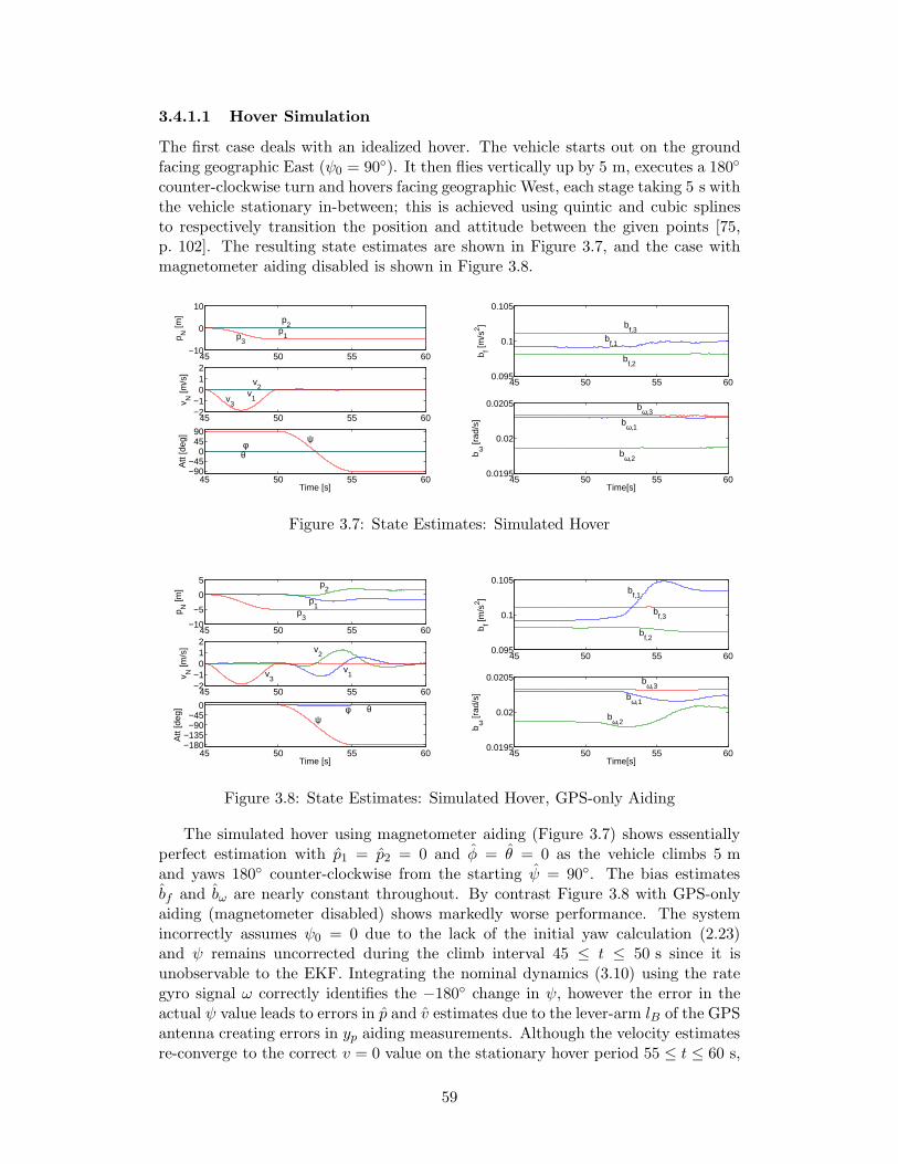
3.4.1.1 Hover Simulation
The first case deals with an idealized hover. The vehicle starts out on the groundfacing geographic East (ψ0 = 90). It then flies vertically up by 5 m, executes a 180
counter-clockwise turn and hovers facing geographic West, each stage taking 5 s withthe vehicle stationary in-between; this is achieved using quintic and cubic splinesto respectively transition the position and attitude between the given points [75,p. 102]. The resulting state estimates are shown in Figure 3.7, and the case withmagnetometer aiding disabled is shown in Figure 3.8.
45 50 55 60−10
0
10
p N [m
]
p1
p2
p3
45 50 55 60−2−1
012
v N [m
/s]
v1
v2
v3
45 50 55 60−90−45
04590
Att
[deg
]
φθ
ψ
Time [s]
45 50 55 600.095
0.1
0.105
b f [m/s
2 ]
bf,1
bf,3
bf,2
45 50 55 600.0195
0.02
0.0205
b ω [r
ad/s
]Time[s]
bω,2
bω,1
bω,3
Figure 3.7: State Estimates: Simulated Hover
45 50 55 60−10
−5
0
5
p N [m
]
p1
p2
p3
45 50 55 60−2−1
012
v N [m
/s]
v1
v2
v3
45 50 55 60−180−135−90−45
0
Att
[deg
] φ θψ
Time [s]
45 50 55 600.095
0.1
0.105
b f [m/s
2 ]
bf,1
bf,3
bf,2
45 50 55 600.0195
0.02
0.0205
b ω [r
ad/s
]
Time[s]
bω,1
bω,2
bω,3
Figure 3.8: State Estimates: Simulated Hover, GPS-only Aiding
The simulated hover using magnetometer aiding (Figure 3.7) shows essentiallyperfect estimation with p1 = p2 = 0 and φ = θ = 0 as the vehicle climbs 5 mand yaws 180 counter-clockwise from the starting ψ = 90. The bias estimatesbf and bω are nearly constant throughout. By contrast Figure 3.8 with GPS-onlyaiding (magnetometer disabled) shows markedly worse performance. The systemincorrectly assumes ψ0 = 0 due to the lack of the initial yaw calculation (2.23)and ψ remains uncorrected during the climb interval 45 ≤ t ≤ 50 s since it isunobservable to the EKF. Integrating the nominal dynamics (3.10) using the rategyro signal ω correctly identifies the −180 change in ψ, however the error in theactual ψ value leads to errors in p and v estimates due to the lever-arm lB of the GPSantenna creating errors in yp aiding measurements. Although the velocity estimatesre-converge to the correct v = 0 value on the stationary hover period 55 ≤ t ≤ 60 s,
59

the p1 and p2 estimates each exhibit a steady-state error of almost 2 m. The biasestimates bf,1 and bω,1, bω,2 are (incorrectly) perturbed at t ≥ 50 s, the start of theturn manoeuver, although the relative importance of this error is smaller than thatfor position, velocity and attitude estimates.
3.4.1.2 Trajectory Simulation
We now consider a more complicated flying trajectory: a three-dimensional figure-8, requiring motion in all six degrees of freedom and producing significant lateralaccelerations due to banking turns. The trajectory is described as a parametriccurve in the navigation frame,
x(t) =M sin(2πt/T ) + x0
y(t) = (m/2) sin(4πt/T ) + y0
z(t) = (−H/2) sin(πt/T ) + z0
(3.27)
where M = 50 m, m = 25 m represent the major and minor diameters of each lobe,respectively, H = 10 m is the total vertical height of the trajectory, T = 50 s isthe period of one complete figure-8 circuit and (x0, y0, z0) = (0, 0,−15) m are theNED coordinates of the geometric center of the trajectory. We define the associatedattitude such that the yaw corresponds to direction of travel, pitch is proportionalto rate of climb, and roll to the turning rate:
ψ(t) = atan2(y′(t), x′(t))
θ(t) = −αz′(t)φ(t) = βψ′(t),
(3.28)
where α = 1, β = 1 are the pitching and banking coefficients, which should be setproportional to the speed of the trajectory, which in turn is inversely proportionalto T . The complete trajectory consists of the initialization period with ψ0 = 90,followed by a 10 s transition to the t = 0 point of (3.27), (3.28) using splines togenerate a smooth transition trajectory as in Section 3.4.1.1, and a 200 s intervalof flying a three-dimensional figure-8 pattern. As in Section 3.4.1.1 we employmagnetometer aiding at Tm = 0.02 s and for comparison consider a GPS-only aideddesign i.e. where magnetometer aiding is disabled.
50 100 150 200 250−50−25
02550
p N [m
] p1 p
2
p3
50 100 150 200 250−8−4
048
v N [m
/s] v
1 v2
v3
50 100 150 200 250−270−180−90
090
Att
[deg
]
φθ
ψ
Time [s]
50 100 150 200 2500.08
0.09
0.1
0.11
0.12
b f [m/s
2 ]
bf,1
bf,2
bf,3
50 100 150 200 2500.016
0.018
0.02
0.022
0.024
b ω [r
ad/s
]
Time[s]
bω,1
bω,2bω,3
Figure 3.9: State Estimates: Simulated figure-8
60

50 100 150 200 250−50−25
02550
p N [m
] p1 p
2
p3
50 100 150 200 250−8−4
048
v N [m
/s] v
1 v2
v3
50 100 150 200 250−270−180−90
090
Att
[deg
]
φθ
ψ
Time [s]
50 100 150 200 2500.08
0.09
0.1
0.11
0.12
b f [m/s
2 ]
bf,1
bf,2
bf,3
50 100 150 200 2500.016
0.018
0.02
0.022
0.024
b ω [r
ad/s
]
Time[s]
bω,1
bω,2
bω,3
Figure 3.10: State Estimates: Simulated figure-8, GPS-only Aiding
The figure-8 trajectory estimation results are shown in Figure 3.9 for the mag-plus-GPS aided INS case and in Figure 3.10 for the GPS-only case. The clearestdifference between the plots is the ψ estimate, which is initially 90 in error inthe GPS-only case but slowly converges to the same trajectory as the mag-aidedcase due to the lateral accelerations providing observability of δγ3 as discussed inSection 3.2.6.2. The magnetometer-aided case provides superior estimation perfor-mance. This is clearly seen in Figure 3.11 where the errors of all 15 estimated statesfrom their reference trajectories are shown for both designs.
−202
∆pN
−303
∆vN
−90
30
∆Att
−0.020
0.02
∆bf
50 100 150 200 250−4
04x 10
−3
∆bω
Time [s]
−202
∆pN
−303
∆vN
−90
30
∆Att
−0.020
0.02
∆bf
50 100 150 200 250−4
04x 10
−3
∆bω
Time [s]
Figure 3.11: State Estimation Errors: Simulated figure-8, Mag-plus-GPS vs GPS-only Aiding
3.4.2 Experimental Ground Test Results
We now turn our attention to experimental results. In the first test, the engine-offhelicopter was manually carried around the perimeter of a rectangular landing padset up at the ERCHA flight field mentioned in Section 2.8. The vehicle was pickedup at the southern-most corner of the pad, kept pointed in the direction of travel,executed a stop and 90 counter-clockwise turn at each corner, and was set downat the start point after two complete circuits. The sensor readings from the IMU,magnetometer and GPS were logged to disk and input into the Aided INS using theengine-off magnetometer calibration constants in Table 2.1 and the data in Table 3.1as the EKF parameters.
61

3.4.2.1 Full versus Yaw-only Magnetometer Aiding
In our initial experiments, we used 3-axis magnetometer readings, compensatedusing the parameters in Table 2.1, as an aiding measurement via the linearizederror system’s output matrix H in (3.17). The resulting state estimates are plottedin Figure 3.12. The position estimates are qualitatively correct: a plot of p2 vs p1traces out the rectangular shape of the landing pad, while p3 correctly identifiesthe pickup and put-down events. Similarly, the estimated roll and pitch φ, θ areheld close to zero, with oscillations created by the gait of the operator carrying thehelicopter, while the estimated yaw ψ increases by π/2 at each corner. However,we see problems in the velocity estimates, which incorrectly estimate a non-zerovelocity before and after the helicopter is carried.
40 60 80 100 120 140 160−10
0
10
20
p N [m
] p1
p2
p3
40 60 80 100 120 140 160−2
0
2
v N [m
/s]
v1
v2v
3
40 60 80 100 120 140 160−200
0
200
Att
[deg
]
Time [s]
φθ
ψ
Start End
40 60 80 100 120 140 160−0.2
0
0.2
0.4
0.6
b f [m/s
2 ] bf,1
bf,2
bf,3
40 60 80 100 120 140 160−0.02
−0.01
0
0.01
0.02
0.03b ω
[rad
/s]
Time [s]
bω,1
bω,2
bω,3
45 50 55 60−0.4−0.2
00.2
p N [m
]
p1
p2 p
3
45 50 55 60−1
0123
Att
[deg
]
Time [s]
φ
θ
Figure 3.12: State Estimates: Ground Test, 3-Axis Mag Aiding
The incorrect velocity estimation problem was diagnosed by zooming in on thepre-pickup estimated states, t ≤ 60 s, shown in the bottom plot of Figure 3.12. Theposition estimate p1 is seen to be affected by the incorrect v1 estimate, however thisis mitigated by the EKF, evidenced by the 10 Hz “sawtooth” pattern created by theaiding measurements from the GPS receiver. This bounds the error in the positionestimates. The estimated roll and pitch angles are updated from zero to φ ≈ 1,θ ≈ 2, which is incorrect since the helicopter remains level. Under the initialyaw angle ψ ≈ 50, the helicopter is estimated to be tilting southwards, causingnegative growth of v1 due to the R term in nominal dynamics (3.10). As seen inFigure 3.12, the growth of v1 is bounded due to GPS updates, however it createsjitter in the position estimates and affects the accelerometer bias estimates bf,1, bf,2,which will affect the accuracy of the integration of nominal dynamics (3.10). Thischain of events is caused by the updates of roll and pitch during the pre-pickup stage,created by errors in magnetometer measurements remaining after compensation. Asdiscussed in Section 3.2.6.2, the triaxial magnetometer output equation providesdirect observability of roll and pitch via δγ1 and δγ2, respectively, which cause the
62

residual sensor errors to feed through into φ and θ.
40 60 80 100 120 140 160−10
0
10
20
p N [m
] p1
p2
p3
40 60 80 100 120 140 160−2
0
2
v N [m
/s]
v1
v2
v3
40 60 80 100 120 140 160−200
0
200
Att
[deg
]
Time [s]
φθ
ψ
40 60 80 100 120 140 160−0.2
0
0.2
0.4
0.6
b f [m/s
2 ]
bf,1
bf,2
bf,3
40 60 80 100 120 140 160−0.02
−0.01
0
0.01
0.02
0.03
b ω [r
ad/s
]
Time [s]
bω,1
bω,2
bω,3
45 50 55 60−0.4−0.2
00.2
p N [m
] p1
p2
p3
45 50 55 60−1
0123
Att
[deg
]
Time [s]
φθ
Figure 3.13: State Estimates: Ground Test, Yaw-Only Mag Aiding
The above discussion motivates the switch to a yaw-only magnetometer updateby replacing the 3-axis δym in (3.17) with the yaw-only δym (3.18). The resultingstate estimates are shown in Figure 3.13. We remark the estimated velocities in thepre- and post-carry phases are correct and that the accelerometer bias estimateschange much less. The zoom-in view at the bottom of Figure 3.13 confirms the rolland pitch angles are not corrected, and exhibits smoother position estimates; thesame conclusion was made in [50, p. 36]. We have found the opposite effect in flighttesting, however, which will be covered in Section 3.4.3.
3.4.2.2 Comparison of Calibration Methods
We now compare the performance of calibration methods discussed in Section 2.9in the yaw-only magnetometer updates version of the filter. Using the logged sensordata from the ground test, we compensate the magnetometer readings using inturn the full model (2.26) with engine-off parameters from Table 2.1, hard-ironcompensation, uncompensated (raw) sensor data, and with magnetometer updatesdisabled. The overhead position and yaw angle estimates for each of the four casesare plotted in Figure 3.14. The dimensions of the landing pad and angle w.r.t. truenorth were measured directly and used to generate the reference trajectory. Thereference yaw angle was generated by using the measured yaw angle of the firstvertex and adding π/2 at every corner turn.
The full compensation case gives good navigation filter performance, with theestimated yaw and overhead positions tracking the reference trajectory fairly closely.A part of the tracking error is caused by imperfect alignment of the helicopter withthe edges of the landing pad during the carry. The hard-iron compensation caseshows good performance as well, although the yaw estimates differ from the fullcompensation case, visible in the start and end configurations. Since the same
63

−10 −4 2 8−2
4
10
16
p N,1
[m]
Full
−10 −4 2 8−2
4
10
16Hard−Iron
−10 −4 2 8−2
4
10
16
pN,2
[m]
p N,1
[m]
Raw Sensor
−10 −4 2 8−2
4
10
16
pN,2
[m]
Mag Disabled
50 100 150−200
0
200
ψ [d
eg]
Full
50 100 150−200
0
200Hard−Iron
50 100 150−200
0
200
Time [s]
ψ [d
eg]
Raw Sensor
50 100 150−200
0
200
Time [s]
Mag Disabled
Figure 3.14: Magnetometer Calibration Comparison, Ground Test, Yaw-Only MagAiding: Overhead Position; Yaw Angle
sensor data is used throughout, this discrepancy is necessarily an effect of the com-pensation method. The raw sensor case produces significant error in the yaw esti-mates, which also affects the position estimates due to the antenna lever arm termin δyp equation (3.17). This confirms the assertion from Section 2.9 that uncom-pensated magnetometer readings cannot be trusted. The magnetometer-disabledcase demonstrates the observability of δγ3 under lateral acceleration discussed inSection 3.2.6.2, with the estimated yaw initialized at ψ0 = 0 gradually convergingtowards its reference value once the helicopter starts moving.
3.4.3 Experimental Flight Results
In the second experimental test, the helicopter takes off from the landing pad, hoversin mid-air with a fixed heading angle and then lands, all under control from anexperienced pilot. The ANCL helicopter is equipped with a Futaba GY401 heading-hold gyro [58], standard equipment for R/C helicopters, which regulates the in-flightyaw angle using angular velocity as the sensed output and the tail rotor pitch asthe control input c.f. Section 5.3.3.2. The remaining degrees of freedom are muchless precise; the helicopter is an underactuated and relatively light vehicle beingflown in unsteady wind conditions, making perfectly stationary hover extremelydifficult. This fact will be reflected in the plots below. The estimated states wereused to generate an animated helicopter model, which was compared against arecorded video of the hover flight, giving a qualitative estimate of the accuracy ofthe navigation states.
The running engine creates significant vibration in the airframe, in addition todisturbing the sensed magnetic field. The noise covariances of the accelerometer, rategyro and magnetometer signals were re-computed using IMU sensor data collectedwhile the engine was running, and are listed in Table 3.2. The engine-on parametersin Table 2.1 were used to compensate the magnetometer readings. Due to the fuellimit of the helicopter, we were unable to collect a sufficiently long data set toaccurately analyze bias dynamics using Allan Variance (c.f. Section 6.2.1); instead,the engine-off β and σb parameters in Table 3.1 are re-used. Due to the uncertaintyof the bias dynamics, the entries of the initial covariance matrix P−
0 correspondingto δbf and δbω were experimentally tuned to 1 × 10⁻³ and 1 × 10⁻⁵, respectively,
64

Table 3.2: Modified Noise Parameters – Engine Onσf σω σm
[m/s3/2] [rad/√s] [G/
√s]
0.1748 0.0079 0.004140.2792 0.0124 0.008750.3847 0.0022 0.01042
and the remaining entries of P−0 were tuned to 1× 10⁻³ due to their dependence on
bias estimation via dynamics (3.10).
3.4.3.1 Estimation Results in Flight
As in Section 3.4.2.1, we investigate the performance of 3-axis versus yaw-only mag-netometer updates while keeping the other filter parameters constant. The plots forthe 3-axis case are shown in Figure 3.15. Before take-off, the pilot increases throttleinput to the engine, identified as the spool up in the plots, causing a counter-torqueon the helicopter body which is in turn compensated by the GY401 unit. The dipin ψ represents a “tail wag” effect of the helicopter prior to take-off, observed in theflight video. This is likely caused by integrator wind-up of the GY401 gyro, which isknown to use a PI control law on the sensed yaw angular velocity [58], although theexact details of the algorithm are proprietary. The helicopter takes off, and aftera transient period visible in the plots, a stable hover is established with the yawangle held nearly constant. The remaining states drift around as the pilot activelycompensates for the turbulent atmospheric conditions, with roll and pitch motionsof the helicopter causing motion in the lateral and longitudinal directions, respec-tively. After landing, the start of the engine spool down phase and resulting changein ψ is visible before sensor logging was terminated.
40 60 80 100 120 140 160 180−5
0
5
p N [m
] p1
p2
p3
40 60 80 100 120 140 160 180−2
0
2
v N [m
/s]
v1
v2
v3
40 60 80 100 120 140 160 180−20
020406080
Att
[deg
]
Time [s]
φ
θ
ψ
Take−Off
Land
Spool Up Spool DownHover
40 60 80 100 120 140 160 180−0.2
0
0.2
0.4
0.6
b f [m/s
2 ]
bf,1
bf,2
bf,3
40 60 80 100 120 140 160 180−0.04
0
0.04
0.08
b ω [r
ad/s
]
Time [s]
bω,3bω,2
bω,1
55 60 65 704050607080
Att
[deg
]
ψ
55 60 65 700
1020
Att
[deg
]
Time [s]
φθ
−101
m[G
]
−400
40
f[m/s
2 ]
55 60 65 70−2
02
ω[r
ad/s
]
Time [s]
Figure 3.15: State Estimates: Flight Test, 3-Axis Mag Aiding
In addition to the hover phase, where the yaw angle is known to be nearly
65

constant, we focus on the pre-takeoff phase, with the helicopter’s skids on the groundsuch that φ = θ = 0. A plot of the estimated attitude angles during this phaseis shown at the bottom of Figure 3.15. The tail wag effect discussed above isclearly visible in the plot of ψ. The φ and θ estimates oscillate and exhibit amean value of approximately 2, indicating the attitude estimates are imperfect butbounded. The errors are caused by a combination of factors, including imperfectδγ1 and δγ2 updates from the magnetometer discussed in Section 3.4.2.1, significantnoise levels in the rate gyro measurements feeding through into attitude estimateR via dynamics (3.10), and the unmodeled effect of engine speed changes on theIMU sensor outputs. This last effect is clearly visible in the sensor data plot inFigure 3.15 which exhibits a pronounced change in the measured signals duringengine spool-up. The estimated bias states in Figure 3.15 show the navigation filtercompensates, however we can reasonably expect noise and bias model uncertaintyto create errors in estimated attitudes. In spite of these factors, using the estimatedstates to animate a helicopter model and comparing it against the flight video, wefind the results are in agreement with reality. Design improvements including bettervibration isolation of the avionics unit from the helicopter body, better modeling ofthe engine-on sensor dynamics, and upgrading to a higher-quality IMU can furtherimprove the performance of the system.
Switching to yaw-only magnetometer updates gives results shown in Figure 3.16.Unlike Section 3.4.2, this method provides significantly worse performance, partic-ularly in attitude estimates. The estimated ψ in hover exhibits drift, while the φand θ estimates are visibly different from those in Figure 3.15. The error is par-ticularly evident in the estimated attitudes prior to take-off, shown at the bottomof Figure 3.16, with estimated ψ incorrectly rising during counter-torque, and φapproaching 20 despite the helicopter being level. This issue is discussed below.
40 60 80 100 120 140 160 180−5
0
5
p N [m
]
p1
p2
p3
40 60 80 100 120 140 160 180−2
0
2
v N [m
/s]
v1
v2
v3
40 60 80 100 120 140 160 180−20
020406080
Att
[deg
]
Time [s]
φ
θ
ψ
40 60 80 100 120 140 160 180−0.2
0
0.2
0.4
0.6
b f [m/s
2 ]
bf,1
bf,2
bf,3
40 60 80 100 120 140 160 180−0.04
0
0.04
0.08
b ω [r
ad/s
]
Time [s]
bω,3
bω,2
bω,1
55 60 65 704050607080
Att
[deg
]
ψ
55 60 65 700
1020
Att
[deg
]
Time [s]
φθ
−101
m[G
]
−400
40
f[m/s
2 ]
55 60 65 70−2
02
ω[r
ad/s
]
Time [s]
Figure 3.16: State Estimates: Flight Test, Yaw-Only Mag Aiding
For flight testing, the errors created by imperfect δγ1 and δγ2 updates fromthe magnetometer are negligible compared to the errors resulting from discarding
66

these updates. Of course the error system (3.17) is theoretically fully observablewith yaw-only magnetometer updates, c.f. Section 3.2.6.2, however in practice theattitude updates depend on f− bf which enters as a coefficient of δγ in the dynamicsmatrix of (3.17), and whose accuracy will in turn be affected by noise and biasdynamics model uncertainty. During spool-up, the combination of increasing enginethrottle and angular acceleration of the main rotor leads to a complicated time-varying vibration response of the helicopter, and in Figure 3.16 we can observe aclear correlation between the start of the spool-up period, the increase in f and ωsensor noise levels and their respective estimated biases, and the growth of errorin φ. The error in θ is bounded, likely due to the lever-arm effect of the tail-mounted GPS receiver providing aiding for δγ2, not available for δγ1 resp. φ sincethe GPS antenna is mounted in the vertical mid-plane of the helicopter. The errorin ψ, visible in pre-takeoff as well as in flight, is caused by violating the assumptionφ = φ, θ = θ, i.e. perfect roll and pitch estimates from the navigation filter, whichwas used in Section 3.2.6.2 to derive the yaw-only magnetometer aiding equation.The parameters of the EKF were re-tuned in an effort to reduce the error in θ, φduring spool-up. However, no significant improvement in performance was achieved.It is still feasible that these errors could be reduced by a combination of re-tuning thefilter parameters, using better models of engine-on bias dynamics, and mechanicalvibration isolation of the IMU unit. A practical solution would be to disable theEKF during spool-up given that its performance during flight is comparable to the3-axis magnetometer update. We propose to simply discard the yaw-only aidingdesign for flight testing and rely on the 3-axis version with filter parameters fromSection 3.4.3 for the final set of flight experiments.
3.4.3.2 Comparison of Calibration Methods
We now provide a flight performance comparison of magnetometer calibration meth-ods using 3-axis updates. As in Section 3.4.2.2, we consider four cases: full com-pensation, hard-iron compensation, raw sensor readings and magnetometer disabled.The set of engine-on parameters listed at the beginning of Section 3.4.3 is used. Themag-disabled case is manually initialized at the correct ψ0 initial yaw angle. Theestimation results are plotted in Figure 3.17, and we plot only attitude estimatesdue to their strong dependence on magnetometer aiding.
50 100 150−20
0
20
40
60
Att
[deg
]
Full
φ
θ
ψ
50 100 150−20
0
20
40
60
Hard−Iron
φ
θ
ψ
50 100 150−20
0
20
40
60
Time [s]
Att
[deg
]
Raw Sensor
φ
θ
ψ
50 100 150−100
−80−60−40−20
0204060
Time [s]
Mag Disabled
φ
θψ
Figure 3.17: Magnetometer Calibration Comparison, Flight Test, 3-Axis Mag Aid-ing: Estimated Attitude
67

The full compensation case is the same plot as Figure 3.15, and serves as a refer-ence for the other three. The hard-iron case produces the correct trend in the flightestimates, although the in-flight yaw angle is in error by approximately 10 fromthe fully compensated case. This may be caused by the significant warping of themagnetometer readings which cannot be compensated for by hard-iron calibration,seen by comparing the engine-on ε, ρ parameters in Table 2.1 with ε = 1, ρ = 0for hard-iron compensation. The raw sensor case has higher errors in yaw angle;in addition, the roll and pitch estimates differ from the reference case, caused byδγ1 and δγ2 mag aiding using uncompensated sensor readings. The magnetometer-disabled case shows a complete divergence of ψ, which makes it clear a yaw sensoris critical in hover flights. As expected, the φ and θ estimates behave identically tothe yaw-only mag aiding case in Figure 3.16.
68

Chapter 4
Invariant Observer Design for
Aided Navigation
4.1 Overview
The Extended Kalman Filter covered in Chapter 3 relies on re-linearization of thesystem about its latest trajectory, an ad-hoc approach which works well in practice asseen in Sections 3.3 and 3.4, but which makes it impossible to analyze global stabilityand difficult to quantify the region of attraction of local stability, c.f. [124]. For thisreason a direct nonlinear observer design for aided inertial navigation systems is ofgreat interest to us.
This Chapter focuses on the nonlinear design method of invariant (symmetry-preserving) observers [27, 28]. This approach provides a systematic method to obtaina nonlinear observer structure which possesses the same symmetries (formally de-fined in Section 4.3) as the original model. Using this observer, an invariant versionof the (nonlinear) estimation error dynamics exists which simplifies the process ofchoosing the observer gains. We will demonstrate that both the AHRS and AidedINS treated in Chapter 3 possess the necessary symmetries to make use of the in-variant observer design method. An early version of invariant observer theory [25]treating an example of velocity-aided navigation was in fact the initial motivationfor studying this method.
After considering a motivating example in Section 4.2, we formally define systemsymmetries in Section 4.3 and find them for the AHRS (Section 4.4) and AidedINS (Section 4.5). We cover invariant observer theory in Section 4.6 and deriveinvariant observers for AHRS and Aided INS in Section 4.7 using rotation matricesR ∈ SO(3) (c.f. Section 2.1), a singularity-free one-to-one parametrization of theSO(3) manifold, making the invariant estimation error dynamics amenable to globalstability analysis [88, 38]. With the exception of [28] the invariant observer designsfound in the literature are formulated in terms of unit quaternions q ∈ H, ‖q‖ = 1(c.f. Section 2.7) making a global analysis impossible due to their two-to-one coveringof SO(3) as noted in [27, Ex. 3].
While choosing the gains of an invariant observer is simplified, the process isnon-systematic due to the requirement of stabilizing a nonlinear system using e.g. aLyapunov analysis. We have found a stabilizing design for the AHRS case whichguarantees almost-global stability, c.f. Section 4.8. However for Aided INS a nonlin-
69

ear stabilizing design has not (yet) been found. A natural approach to systematicallyachieving stabilization is to apply the EKF to the nonlinear invariant estimation dy-namics, an approach originally proposed in [23] and termed the Invariant EKF, laterapplied to aided navigation examples in [29, 96]. We introduce the Invariant EKFmethod in Section 4.9 and adapt it to our AHRS and Aided INS examples in a “nat-ural” way, removing the need to formulate the system using invariant noise termsas in [23], c.f. Section 4.9.1. We then provide a comprehensive performance compar-ison of the invariant observers in both simulation and experiment in Sections 4.10and 4.11.
4.2 Motivating Example
Consider the AHRS from Section 3.2.3.1. For simplicity we replace the Gauss-Markov process model of the bias dynamics with the Wiener process model bω = νbω .The nominal version of (3.5), (3.6) is then written as
R = RS(ω − bω)
bω = 0[yaym
]=
[RTaRTm
],
(4.1)
where as before R ∈ SO(3), the rotation matrix from body-fixed to ground-fixedframe, expresses the attitude of the system; S is the skew-symmetric matrix de-fined in (2.2); ω and bω are the measured angular velocity and its bias, respectively,the former available from the on-board rate gyro, the latter an unknown constant;ya and ym are readings from the on-board accelerometer and magnetometer; anda = [0 0 −9.81]T m/s2, m = [BH 0 BV ]
T G represent the ground-frame grav-ity and magnetic field vectors which are known and constant as discussed in Sec-tion 2.8.1. As in Section 3.2.2 we have assumed ya directly measures gravity i.e. zerotranslational acceleration and that ym has been compensated for magnetic field dis-tortions. The task of the AHRS is to estimate attitude R and rate gyro bias bω fromthe signals ω, ya and ym — an observer design problem.
Defining x = (R bω) and u = ω, the nonlinear dynamics (4.1) are written
x = f(x, u) =
(RS(ω − bω)
0
).
Consider the change of variables
x′ =
(RR0
RT0 (bω + ω0)
), u′ = RT0 (ω + ω0) (4.2)
where R0 ∈ SO(3) and ω0 ∈ R3 are constants. We directly verify
f(x′, u′) =
(RR0S
(RT0 (ω + ω0)−RT0 (bω + ω0)
)
0
)
=
(RR0S
(RT0 (ω − bω)
)
0
)=
(RS (ω − bω)R0
0
)
70

andd
dt(x′) =
d
dt
(RR0
RT0 (bω + ω0)
)=
(RR0
RT0 (bω)
)=
(RS(ω − bω)R0
0
),
i.e. x′ = f(x′, u′) under the above change of variables. Similarly, the output in (4.1)
y = h(x) =
(RTaRTm
)
becomes
h(x′) =
((RR0)
Ta(RR0)
Tm
)=
(RT0 R
TaRT0 R
Tm
)=
(RT0 yaRT0 ym
)
which “induces” the change of variables y′ = h(x′) under the definition
y′ =
(RT0 yaRT0 ym
).
System (4.1) can alternatively be written in terms of unit quaternions q ∈ H, ‖q‖ = 1using rotational kinematics (2.21):
q =1
2q ∗ (ω − bω)
bω = 0[yaym
]=
[q−1 ∗ a ∗ qq−1 ∗m ∗ q
],
(4.3)
where ∗ represents quaternion multiplication and q−1 is the quaternion inverse;the R
3 vectors ω − bω, a and m are understood to be taken as pure quaternionsv = (0, ~v) when multiplying q. Denoting the dynamics of (4.3) as x = f(x, u) wherex = (q bω) and u = ω, consider the change of variables
x′ =
(q ∗ q0
q−10 ∗ (bω + ω0) ∗ q0
), u′ = q−1
0 ∗ (ω + ω0) ∗ q0
where q0 ∈ H, ‖q0‖ = 1 and ω0 ∈ R3 are constants, we directly verify
f(x′, u′) =1
2q ∗ q0 ∗
(q−10 ∗ (ω + ω0) ∗ q0 − q−1
0 ∗ (bω + ω0) ∗ q0)
=1
2q ∗ q0 ∗
(q−10 ∗ (ω − bω) ∗ q0
)
=1
2q ∗ (ω − bω) ∗ q0
and
d
dt(x′) =
d
dt
(q ∗ q0
q−10 ∗ (bω + ω0) ∗ q0
)=
(q ∗ q0
q−10 ∗ bω ∗ q0
)=
1
2
(q ∗ (ω − bω) ∗ q0
0
),
so once again x′ = f(x′, u′) under the proposed change of variables. The outputin (4.3)
y = h(x) =
[q−1 ∗ a ∗ qq−1 ∗m ∗ q
]
71

transforms to
h(x′) =
[(q ∗ q0)−1 ∗ a ∗ q ∗ q0(q ∗ q0)−1 ∗m ∗ q ∗ q0
]=
[q−10 ∗ q−1 ∗ a ∗ q ∗ q0q−10 ∗ q−1 ∗m ∗ q ∗ q0
]=
[q−10 ∗ ya ∗ q0q−10 ∗ ym ∗ q0
]
and induces the change of variables
y′ =
[q−10 ∗ ya ∗ q0q−10 ∗ ym ∗ q0
]
such that y′ = h(x′).We have directly verified that the AHRS equations (4.1) or (4.3) are invariant
with respect to certain changes of variables to x, u and y; we refer to these changesas the symmetries of the system. The mathematical details of the transformationsare quite different for the two cases, however they represent the same symmetries:the transformed state x′ corresponds to rotating the body-fixed axes by R0 or q0,and adding the constant ω0 to the sensor bias. Provided that u = ω, the sensedangular velocity in the body-fixed frame, is also transformed by R0 or q0 and ω0,we intuitively expect the governing dynamics to remain the same, which is verifiedabove. The same physical interpretation applies to the output y′. We have seenthat invariance is independent of the attitude parametrization used, and the the-ory will be formulated using the framework of differential geometry to make thisindependence precise.
For a system with symmetries, there exists a constructive method to be coveredin Section 4.6 to build a (nonlinear) observer which possess the same symmetriesas the system. The resulting estimation error dynamics possess a reduced-orderform which simplifies stability analysis and gain selection, c.f. Section 4.6.3. Wework with the same two examples as in Chapter 3 using a Wiener process model forthe bias dynamics: the AHRS (4.1), and the Magnetometer-plus-GPS-Aided INSintroduced in Section 3.2.3.2 whose symmetries will be provided in Section 4.5.
4.3 System Symmetries
The coordinate-free formulation of the smooth (C∞) nonlinear control system x =f(x, u) is the commutative diagram [107, Sec. 13.5]
BF
//
π A
AAAA
AAA TM
πM||yyyyyyyy
M
(4.4)
where B is the total space of a smooth fiber bundle over M equipped with thesurjective map π : B → M , TM is the tangent bundle of M with the naturalprojection map πM : TM → M , and F : B → TM is a bundle map, also knownas a bundle morphism. By definition of a smooth fiber bundle, B, M and TMare smooth manifolds and π, F and πM are smooth maps. The base manifold Mrepresents the state space of the system, and for each x ∈M , the fiber π−1(x) ⊂ Brepresents a state-dependent input space. In this way, diagram (4.4) can describe
72

the dynamics of systems under state feedback, and is used in e.g. [129, 63] to definesystem symmetry as the commutativity of
Bθg
//
F
""EEE
EEEE
E
π
BF
||yyyyyyyy
π
TM(ϕg)∗
//
πM||yyyyyyyy
TM
πM""E
EEEE
EEE
M ϕg
//M
(4.5)
where θg, ϕg are group actions of a Lie group G ∋ g on the manifolds B and M ,respectively, and (ϕg)∗ denotes the pushforward of the map ϕg.
We briefly elaborate on how (4.4) relates to the usual x = f(x, u) coordinatedynamics. A smooth fiber bundle consists of a smooth manifold B together witha surjective smooth map π onto the smooth manifold M . For each x ∈ M , thereexists a neighbourhood U of x and a diffeomorphism Φ : π−1(U) → U × V , whereV is a smooth manifold, such that the following diagram commutes:
π−1(U)Φ
//
π##G
GGGG
GGGG
U × V
π1||yyyyyyyyy
U
where π1 is the projection on the first factor. The smooth manifolds B, M and Vare known as the total space, base space and standard fiber, respectively, and Φ isthe local trivialization of B over U . For any x0 ∈ M and b0 ∈ π−1(x0) ⊂ B, wehave the coordinate functions (x1, . . . , xn, u1, . . . , um) = (x, u) around Φ(b0), suchthat (x, u) is a local coordinate expression for the total space B. Returning to (4.4),the standard coordinates for TM are written as (x1, . . . , xn, v1, . . . , vn) = (x, v),where x are the same coordinate functions around x0 ∈ M as above, and v are thecoordinate representations of the component functions of the vector field describedby F : B → TM , given by the right-hand side of x = f(x, u). In other words,the coordinate representation of F : B → TM is given by F (x, u) = (x, f(x, u))which recovers the dynamics x = f(x, u). As seen in (4.1), (4.3), two coordinaterepresentations of F may look very different from each other.
Because inputs to the observer are not directly functions of its state, we are ableto take the total space B in (4.4) as the product manifold B =M ×V , making B atrivial fiber bundle over M , where the standard fiber V is the input manifold whichis independent of the state manifold M . Remark this simplification does not applyto invariant controller design problems [120, 90, 47].
Using the trivial bundle B = M × V , take ϕg : G × M → M and ψg : G ×V → V to be smooth Lie group actions (c.f. Section 4.3.1) acting on the system’sstate and input manifolds, respectively, where G is the Lie group associated tothe system known as its symmetry group. We define the system dynamics to beG-invariant [90, 27] if
(ϕg)∗F (x, u) = F (ϕg(x), ψg(u)) ∀g ∈ G,
73

a coordinate-free definition which is consistent with the general symmetry caseshown in (4.5). In local coordinates, this is equivalent to
d
dt(ϕg(x)) = f(ϕg(x), ψg(u)) ∀g ∈ G,
or simply x′ = f(x′, u′), the change of variables used in Section 4.2. Similarly, forthe output map H :M×V → Y where Y is the output manifold, the system outputis G-equivariant if
ρgH(x, u) = H(ϕg(x), ψg(u)) ∀g ∈ G,
where ρg : G × Y → Y is a Lie group action on the output manifold Y , which is“induced” by ϕg and ψg as seen in Section 4.2. The coordinate version of this is
ρgy = h(ϕg(x), ψg(u)) ∀g ∈ G,
or equivalently y′ = h(x′, y′). The set of Lie group actions (ϕg, ψg, ρg) which verifiesa system’s G-invariance and G-equivariance are known as its symmetries.
The concept of invariance appears in standard differential geometry referencesin the following context (e.g. [83, p. 93]): let G be a Lie group, and define lefttranslation Lg : G×G→ G as the map Lg(h) = gh. A vector field Xg : G→ TG issaid to be left-invariant if
(Lg′)∗Xg = Xg′g ∀g, g′ ∈ G.
The G-invariance of a system defined above can be viewed as a generalization ofthis definition, and we will see further links between the two in Section 4.6.2. Onthe other hand, equivariance is a standard concept and applies exactly as above,e.g. [83, p. 212].
4.3.1 Lie Group Actions
A Lie group action θg : G×M →M can be either left or right. A left group actionθg verifies
θg1 θg2(p) = θg1g2(p) ∀g1, g2 ∈ G,∀p ∈M
θe(p) = p ∀p ∈M
while a right group action θg verifies
θg2 θg1(p) = θg1g2(p) ∀g1, g2 ∈ G,∀p ∈M
θe(p) = p ∀p ∈M
We deal exclusively with smooth Lie group actions, meaning θg : G×M →M is asmooth map for all g ∈ G and p ∈ M . Under this assumption, the inverse θg−1 foreither action type is smooth, making θg a diffeomorphism.
For our purposes, we will always work with ϕg, ψg, ρg as being left Lie groupactions. We will demonstrate that this is done by correctly defining the group mul-tiplication g1g2 ∈ G. The reason for this is that two steps in the invariant observerdesign, finding the group invariants (Section 4.6.1) and building an invariant frame(Section 4.6.2) assume a left Lie group action is being used. Although the procedurecould be modified to use the right group action case, there is nothing to be gainedfrom doing so. In the sequel, any Lie group action is understood to be left unlessexplicitly stated otherwise.
74

4.4 AHRS symmetries
Return to the AHRS in Section 4.2, using version (4.1) written in terms of rotationmatrices. Let G = SO(3) × R
3 be the Lie group acting on x = (R bω), u = ω,y = (ya ym), and let g = (R0 ω0) ∈ G. The changes of variables were actuallythe Lie group actions
ϕg
(Rbω
)=
(RR0
RT0 (bω + ω0)
), ψg
(ω)=(RT0 (ω + ω0)
), ρg
(yaym
)=
(RT0 yaRT0 ym
).
Clearly, for g = e = (I, 0) ∈ G, ϕe(x) = x, ψe(u) = u and ρe(y) = y. In order tomeet the left group action assumption in Section 4.3.1, we require ϕg1 ϕg2 = ϕg1g2 .Consider g1 = (R′
0, ω′0) ∈ G and g2 = (R′′
0 , ω′′0 ) ∈ G. We compute
ϕg1 ϕg2(Rbω
)= ϕg1
(RR′′
0
(R′′0)T (bω + ω′′
0)
)=
(RR′′
0R′0
(R′0)T (R′′
0)T (bω + ω′
0 + ω′′0)
)
based on which we define group multiplication g1g2 = (R′′0R
′0, ω
′0 + ω′′
0 ) ∈ G, underwhich
ϕg1g2
(Rbω
)=
(RR′′
0R′0
(R′′0R
′0)T (bω + ω′
0 + ω′′0)
)
proving ϕg is a left action. Continuing with the input action ψg, we verify
ψg1 ψg2(ω)= ψg1
((R′′
0)T (ω + ω′′
0))= (R′
0)T (R′′
0)T (ω + ω′
0 + ω′′0)
andψg1g2
(ω)= (R′′
0R′0)T (ω + ω′
0 + ω′′0) = (R′
0)T (R′′
0)T (ω + ω′
0 + ω′′0)
hence ψg is also a left action. Finally, for the output action
ρg1 ρg2(yaym
)= ρg1
((R′′
0)T ya
(R′′0)T ym
)=
((R′
0)T (R′′
0)T ya
(R′0)T (R′′
0)T ym
)
and
ρg1g2
(yaym
)=
((R′′
0R′0)T ya
(R′′0R
′0)T ym
)=
((R′
0)T (R′′
0)T ya
(R′0)T (R′′
0)T ym
)
hence ρg is a left action as well. Using the more “natural” multiplication definitiong1g2 = (R′
0R′′0 , ω
′0+ω′′
0) ∈ G can be directly verified to yield right actions ϕg, ψg, ρgwhich are not suitable for our use. Note the Lie group actions ϕg, ψg, ρg can alsobe taken as acting on (4.3) by writing them in terms of unit quaternions, resultingin different calculation details but the same results as above, c.f. [91].
4.4.1 Ground frame symmetries
The AHRS symmetries considered so far physically represent the rotation of thebody-fixed frame. A different set of symmetries can be obtained by consideringrotations of the ground-fixed frame. Consider system (4.1) and take x = (R bω),u = (ω a m), i.e. treat the ground-frame magnetic and gravity fields as additionalinputs to the system. Let G = SO(3) × R
3 ∋ (Q0, ω0) = g be the symmetry group
75

of the system where Q0 represents a constant rotation of the ground-fixed frame.Defining the Lie group actions
Φg
(Rbω
)=
(Q0Rω0 + bω
), Ψg
ωam
=
ω0 + ωQ0aQ0m
,
we verify
f(Φg(x),Ψg(u)
)=
(Q0RS(ω0 + ω − ω0 − bω)
0
)=
(Q0RS(ω − bω)
0
)
d
dt
(Φg(x)
)=
d
dt
(Q0Rω0 + bω
)=
(Q0RS(ω − bω)
0
),
and so the dynamics are invariant w.r.t. Φg, Ψg. These induce the output action Υg
as
Υg
(yaym
)= h
(Φg(x),Ψg(u)
)=
((Q0R)
TQ0g(Q0R)
TQ0m
)=
(RT gRTm
)=
(yaym
)=⇒ Υg = Id
Let g1 = (Q′0, ω
′0), g2 = (Q′′
0 , ω′′0) and compute
Φg1 Φg2(Rbω
)= Φg1
(Q′′
0Rω′′0 + bω
)=
(Q′
0Q′′0R
ω′0 + ω′′
0 + bω
)
from which we define g1g2 = (Q′0Q
′′0, ω
′0 + ω′′
0) to make Φg a left group action:
Φg1g2
(Rbω
)=
(Q′
0Q′′0R
ω′0 + ω′′
0 + bω
)
Remark that the g1g2 definition happens to use a “natural” multiplication orderQ′
0Q′′0 . Considering Ψg, we have
Ψg1g2
ωam
=
ω′0 + ω′′
0 + ωQ′
0Q′′0a
Q′0Q
′′0m
and
Ψg1 Ψg2
ωam
= Ψg1
ω′′0 + ωQ′′
0aQ′′
0m
=
ω′0 + ω′′
0 + ωQ′
0Q′′0a
Q′0Q
′′0m
,
verifying Ψg is a left action. Finally, Υg = Id is a trivial Lie group action which isleft (or right). We have thus shown that the AHRS example (4.1) is G-invariant andG-equivariant w.r.t. the Lie group actions Φg, Ψg, Υg, which physically representrotations of the ground-fixed reference frame.
4.4.2 Combined symmetries
Since the body and ground-fixed frames can be rotated independently of each other,it’s logical to construct a set of combined symmetries containing both Q0 and R0
terms. Consider (4.1) with x = (R bω), u = (ω a m) and y = (ya ym) as
76

the state, input and output spaces, respectively, and define the symmetry groupG = SO(3) × SO(3) × R
3 ∋ (Q0, R0, ω0) = g, where Q0 and R0 represent rotationsof the ground and body frames, respectively. The candidate Lie group actions forthis case are
ξg
(Rbω
)=
(Q0RR0
RT0 (bω + ω0)
), υg
ωam
=
RT0 (ω + ω0)
Q0aQ0m
,
and we directly verify system invariance:
f(ξg(x), υg(u)
)=
(Q0RR0S
[RT0 (ω + ω0)−RT0 (bω + ω0)
]
0
)=
(Q0RS(ω − bω)R0
0
)
d
dt
(ξg(x)
)=
d
dt
(Q0RR0
RT0 (bω + ω0)
)=
(Q0RS(ω − bω)R0
0
)
The induced output action g is
h(ξg(x), υg(u)
)=
((Q0RR0)
TQ0a(Q0RR0)
TQ0m
)=
(RT0 yaRT0 ym
)=⇒ g
(yaym
)=
(RT0 yaRT0 ym
)
Take g1 = (Q′0, R
′0, ω
′0) ∈ G, g2 = (Q′′
0 , R′′0 , ω
′′0 ) ∈ G. We have
ξg1 ξg2(Rbω
)= ξg1
(Q′′
0RR′′0
(R′′0)T (bω + ω′′
0 )
)=
(Q′
0Q′′0RR
′′0R
′0
(R′0)T (R′′
0)T (bω + ω′
0 + ω′′0 )
),
and thus define g1g2 = (Q′0Q
′′0, R
′′0R
′0, ω
′0+ω′′
0) such that ξg1 ξg2 = ξg1g2 . The inputaction υg verifies
υg1g2
ωam
=
(R′′
0R′0)T (ω + ω′
0 + ω′′0)
Q′0Q
′′0a
Q′0Q
′′0m
and
υg1 υg2
ωam
= υg1
(R′′
0)T (ω + ω′′
0)Q′′
0aQ′′
0m
=
(R′
0)T (R′′
0)T (ω + ω′
0 + ω′′0)
Q′0Q
′′0a
Q′0Q
′′0m
,
while the output action g verifies
g1g2
(yaym
)=
((R′′
0R′0)T ya
(R′′0R
′0)T ym
)
and
g1 g2(yaym
)= g1
((R′′
0)T ya
(R′′0)T ym
)=
((R′
0)T (R′′
0)T ya
(R′0)T (R′′
0)T ym
)
so ξg, υg, g are left Lie group actions as required. Remark that by taking Q0 = Ior R0 = I the actions reduce to (ϕg, ψg, ρg) and (Φg,Ψg,Υg), respectively.
77

4.5 Aided INS Symmetries
The second example to be treated is the Magnetometer-plus-GPS-Aided INS intro-duced in Section 3.2.3.2. As in Section 4.2 we take the bf and bω bias dynamicsmodels as a Wiener process b = ν. The nominal version of Aided INS dynamics (3.9)becomes
p = v
v = R(f − bf )− a
R = RS(ω − bω)
bf = 0
bω = 0
(4.6)
where p, v are the position and velocity of the vehicle relative to the navigation frameorigin, R ∈ SO(3) measures its attitude and bf , bω are the constant, unknown biasesof the specific force f and angular velocity ω signals measured by the on-board IMU.The outputs of the system are
yp = p
ym = RTm(4.7)
where yp and ym are measured by a GPS receiver and magnetometer, respectively;for simplicity, we have taken the vehicle’s position p as directly measurable, whichassumes the rotation matrix RNE and navigation frame location roE have been found(c.f. Section 2.4). The vector m = [Bx By Bz]
T is the navigation frame magneticfield which is known and constant (c.f. Section 2.8) and ym is assumed to have beencompensated for magnetic field distortions as in Section 3.2.2.
The state of (4.6), (p v R bf bω) ∈ R3 × R
3 × SO(3) × R3 × R
3 = M is asmooth manifold and we take the symmetry group G = R
3 × SO(3) × R3 × R
3 ∋(p0 R0 bf0 bω0). We propose the Lie group actions
ϕ(p0,R0,bf0,bω0)
pvRbfbω
=
p+ p0v
RR0
RT0 (bf + bf0)RT0 (bω + bω0)
, ψ(p0,R0,bf0,bω0)
(fω
)=
(RT0 (f + bf0)RT0 (ω + bω0)
)
from which we directly verify
f(ϕg(x), ψg(u)
)=
vRR0
[RT0 (f + bf0)−RT0 (bf + bf0)
]− a
RR0S[RT0 (ω + bω0)−RT0 (bω + bω0)
]
00
=
vR(f − bf )− aRS(ω − bω)R0
00
d
dtϕg(x) =
d
dt
p+ p0v
RR0
RT0 (bf + bf0)RT0 (bω + bω0)
=
pv
RR0
RT0 bfRT0 bω
=
vR(f − bf )− aRS(ω − bω)R0
00
78

and so the system is G-invariant. We then find ρg which makes the system G-equivariant:
h(ϕg(x), ψg(u)) =
(p+ p0
(RR0)Tm
)=⇒ ρ(p0,R0,bf0,bω0)
(ypym
)=
(yp + p0RT0 ym
)
Next, we must define the group multiplication on G making ϕg, ψg, ρg left Lie groupactions. Let g1 = (p′0 R′
0 b′f0 b′ω0) and g2 = (p′′0 R′′0 b′′f0 b′′ω0). We have
ϕg1 ϕg2
pvRbfbω
= ϕg1
p+ p′′0v
RR′′0
(R′′0)T (bf + b′′f0)
(R′′0)T (bω + b′′ω0)
=
p+ p′0 + p′′0v
RR′′0R
′0
(R′0)T (R′′
0)T (bf + b′f0 + b′′f0)
(R′0)T (R′′
0)T (bω + b′ω0 + b′′ω0)
and so define g1g2 = (p′0 + p′′0 R′′0R
′0 b′f0 + b′′f0 b′ω0 + b′′ω0) such that
ϕg1g2
pvRbfbω
=
p+ p′0 + p′′0v
RR′′0R
′0
(R′′0R
′0)T (bf + b′f0 + b′′f0)
(R′′0R
′0)T (bω + b′ω0 + b′′ω0)
= ϕg1 ϕg2
pvRbfbω
.
The input action ψ is left:
ψg1 ψg2(fω
)= ψg1
((R′′
0)T (f + b′′f0)
(R′′0)T (ω + b′′ω0)
)=
((R′
0)T (R′′
0)T (f + b′f0 + b′′f0)
(R′0)T (R′′
0)T (ω + b′ω0 + b′′ω0)
)
and
ψg1g2
(fω
)=
((R′′
0R′0)T (f + b′f0 + b′′f0)
(R′′0R
′0)T (ω + b′ω0 + b′′ω0)
)
The output action ρ is also left:
ρg1 ρg2(ypym
)= ρg1
(yp + p′′0(R′′
0)T ym
)=
(yp + p′0 + p′′0
(R′0)T (R′′
0)T ym
)
and
ρg1g2
(ypym
)=
(yp + p′0 + p′′0(R′′
0R′0)T ym
)
Instead of rotating the body-fixed frame as above, we can rotate the ground-fixed frame by Q0, such that the symmetry group G = R
3 × SO(3)×R3 ×R
3 withG ∋ (p0, Q0, bf0, bω0) = g acts on the state and input manifolds respectively by Φgand Ψg:
Φ(p0,Q0,bf0,bω0)
pvRbfbω
=
Q0(p0 + p)Q0vQ0R
bf0 + bfbω0 + bω
, Ψ(p0,Q0,bf0,bω0)
fωam
=
bf0 + fbω0 + ωQ0aQ0m
,
79

We directly verify the G-invariance of (4.6) to Φg and Ψg:
f(Φg(x),Ψg(u)
)=
Q0vQ0R (f + bf0 − bf − bf0)−Q0aQ0RS (ω + bω0 − bω − bω0)
00
=
Q0vQ0R (f − bf )−Q0aQ0RS (ω − bω)
00
d
dtΦg(x) =
d
dt
Q0(p0 + p)Q0vQ0R
bf0 + bfbω0 + bω
=
Q0vQ0 [R(f − bf )− a]Q0RS(ω − bω)
00
,
and find the induced output action Υg:
h(Φg(x),Ψg(u)
)=
(Q0(p0 + p)(Q0R)
TQ0m
)=⇒ Υg
(ypym
)=
(Q0(p0 + yp)
ym
).
Take g1 = (p′0 Q′0 b′f0 b′ω0) and g2 = (p′′0 Q′′
0 b′′f0 b′′ω0). We have
Φg1 Φg2
pvRbfbω
= Φg1
Q′′0(p + p′′0)Q′′
0vQ′′
0Rbf + b′′f0bω + b′′ω0
=
Q′0Q
′′0(p+ p′0 + p′′0)Q′
0Q′′0v
Q′0Q
′′0R
bf + b′f0 + b′′f0bω + b′ω0 + b′′ω0
and defining g1g2 = (p′0 + p′′0, Q′0Q
′′0, b
′f0 + b′′f0, b
′ω0 + b′′ω0) verifies Φg1 Φg2 = Φg1g2 :
Φg1g2
pvRbfbω
=
Q′0Q
′′0(p + p′0 + p′′0)Q′
0Q′′0v
Q′0Q
′′0R
bf + b′f0 + b′′f0bω + b′ω0 + b′′ω0
We also verify Ψg1 Ψg2 = Ψg1g2 for the input action:
Ψg1 Ψg2
fωam
= Ψg1
f + b′′f0ω + b′′ω0Q′′
0aQ′′
0m
=
f + b′f0 + b′′f0ω + b′ω0 + b′′ω0
Q′0Q
′′0a
Q′0Q
′′0m
= Ψg1g2
fωam
and Υg1 Υg2 = Υg1g2 for the output action:
Υg1 Υg2
(ypym
)= Υg1
(Q′′
0(yp + p′′0)ym
)=
(Q′
0Q′′0(yp + p′0 + p′′0)
ym
)= Υg1g2
(ypym
)
This confirms Φg, Ψg and Υg are left group actions.As in Section 4.4.2, we consider the combined case of rotating both the body and
the ground frames. The symmetry group is G = R3 × SO(3) × SO(3) × R
3 × R3 ∋
80

(p0 Q0 R0 bf0 bω0) = g and the state and input actions are
ξg
pvRbfbω
=
Q0(p+ p0)Q0v
Q0RR0
RT0 (bf + bf0)RT0 (bω + bω0)
, υg
fωam
=
RT0 (f + bf0)RT0 (ω + bω0)
Q0aQ0m
which verify f(ξg(x), υg(u)
)= d/dt(ξg(x)),
f(ξg(x), υg(u)
)=
Q0vQ0RR0
[RT0 (f + bf0)−RT0 (bf + bf0)
]−Q0a
Q0RR0S[RT0 (ω + bω0)−RT0 (bω + bω0)
]
00
d
dtξg(x) =
d
dt
Q0(p+ p0)Q0v
Q0RR0
RT0 (bf + bf0)RT0 (bω + bω0)
=
Q0vQ0 [R(f − bf )− a]Q0RS(ω − bω)R0
00
and induce the output action g
h(ξg(x), υg(u)
)=
(Q0(p+ p0)
(Q0RR0)TQ0m
)=⇒ g
(ypym
)=
(Q0(yp + p0)RT0 ym
).
Take g1 = (p′0 Q′0 R′
0 b′f0 b′ω0) and g2 = (p′′0 Q′′0 R′′
0 b′′f0 b′′ω0). We have
ξg1 ξg2
pvRbfbω
= ξg1
Q′′0(p + p′′0)Q′′
0vQ′′
0RR′′0
(R′′0)T (bf + b′′f0)
(R′′0)T (bω + b′′ω0)
=
Q′0Q
′′0(p+ p′0 + p′′0)Q′
0Q′′0v
Q′0Q
′′0RR
′′0R
′0
(R′0)T (R′′
0)T (bf + b′f0 + b′′f0)
(R′0)T (R′′
0)T (bω + b′ω0 + b′′ω0)
and so we define group multiplication as g1g2 = (p′0 + p′′0, Q′0Q
′′0, R
′′0R
′0, b
′f0 +
b′′f0, b′ω0 + b′′ω0) such that ξg1 ξg2 = ξg1g2 :
ξg1g2
pvRbfbω
=
Q′0Q
′′0(p + p′0 + p′′0)Q′
0Q′′0v
Q′0Q
′′0RR
′′0R
′0
(R′′0R
′0)T (bf + b′f0 + b′′f0)
(R′′0R
′0)T (bω + b′ω0 + b′′ω0)
We verify υg1 υg2 = υg1g2
υg1 υg2
fωam
= υg1
(R′′0)T (f + b′′f0)
(R′′0)T (ω + b′′ω0)Q′′
0aQ′′
0m
=
(R′0)T (R′′
0)T (f + b′f0 + b′′f0)
(R′0)T (R′′
0)T (ω + b′ω0 + b′′ω0)Q′
0Q′′0a
Q′0Q
′′0m
υg1g2
fωam
=
(R′′0R
′0)T (f + b′f0 + b′′f0)
(R′′0R
′0)T (ω + b′ω0 + b′′ω0)Q′
0Q′′0a
Q′0Q
′′0m
81

and g1 g2 = g1g2
g1 g2(ypym
)= g1
(Q′′
0(yp + p′′0)(R′′
0)T ym
)=
(Q′
0Q′′0(yp + p′0 + p′′0)
(R′0)T (R′′
0)T ym
)
g1g2
(ypym
)=
(Q′
0Q′′0(yp + p′0 + p′′0)(R′′
0R′0)T ym
)
so ξg, υg, g are left actions.
4.6 Invariant Observer Theory
4.6.1 Invariants and Moving Frame
Using notation from Section 4.4 define the Lie group action φg = ϕg × ψg × ρgof the symmetry group G acting on the smooth manifold M = X × V × Y withdim(M) = m, dim(G) = r and r ≤ m. A real-valued function J :M → R is definedto be an invariant of G [110, p. 77] if
J(φg(p)) = J(p) ∀g ∈ G, ∀p ∈M
We will cover an algorithm for obtaining the complete set of invariants of G whichare used in Sections 4.6.2 and 4.6.3 below. This procedure uses a moving framewhich is obtained using the constructive method in [52, 112].
We first review some definitions associated with Lie group actions:
• The orbit Op of p ∈M is the set φg(p) : g ∈ G
• G acts semi-regularly on M if the orbits Op all have the same dimension
• G acts regularly on M if it acts semi-regularly and in addition, each p ∈ Mhas arbitrarily small neighborhoods U ⊂M whose intersection with each orbitin M is a connected subset of the orbit
• The action φg is transitive if for every p ∈M , Op =M
• The isotropy group Gp of p ∈M is the set g ∈ G : φg(p) = p
• An action φg is free if for every p ∈M , Gp = e
• An action φg is locally free if for every p ∈M , Gp is a discrete subgroup of G
We deal exclusively with regular Lie group actions; the additional conditions oversemi-regular actions are easily satisfied except for pathological cases e.g. [112, p. 158],and in exchange much stronger results can be proven specifically the followingadapted from [111, Thm. 2.23]:
Theorem 1 Let G be a Lie group acting regularly on an m-dimensional manifoldM with s-dimensional orbits. Then, around every point p0 ∈ M , there exists a“flat” chart U with local coordinates (y, z) = (y1, . . . , ys, z1, . . . , zm−s), such thatany orbit Op intersects U either in the empty set, or in a single s-slice S ⊂ Udefined in coordinates as S = (y, z)|(z1 = c1, . . . , zm−s = cm−s for some c =(c1, . . . , cm−s) ∈ R
m−s.
82

Remark : This says that the “flat” coordinate functions zi : U → R are constantalong any orbit passing through U ⊂ M . The actual set of values c is different forevery orbit, and can be used to (locally) distinguish between them. Because eachorbit is the set of points φg(p) : g ∈ G, the flat coordinate functions define aset of (m − s) invariants of G, (J1(x), . . . , Jm−s(x)) = (z1, . . . , zm−s), which existin a neighborhood U around any point p0 ∈ M . Any other invariant J(x) can beuniquely expressed as an analytic function of this set [112, Thm. 8.17]: J(x) =H(J1(x), . . . , Jm−s(x)). Note that although the theorem guarantees existence of theflat charts, it says nothing about how to actually find their local coordinates; thisis done using the constructive method of normalization discussed below.
Theorem 1 is a consequence of the Frobenius Theorem, used to prove that aLie group acting smoothly with constant rank forms a foliation of the manifoldM , where the leaves are the individual orbits. Semi-regular actions (i.e. acting withconstant rank) are sufficient to prove existence of the foliation and its associated flatcharts, however the intersection may occur in a countable union of s-slices, whichis why we demand the action to be regular. A proof of the Frobenius Theorem andthe existence of foliation is given in [83, Chap. 19].
Theorem 1 can be visualized by considering a simple example. Consider theLie group of planar rotations SO(2) acting on R
2, a smooth manifold. We knowSO(2) acts regularly on R
2\0 [112, p. 162]. The orbits of SO(2) on R2 are circles
centered at the origin shown schematically in Figure 4.1, and the dimension of eachorbit is 1. Consider the chart of polar coordinates on R
2 with U = R2\0 and
coordinate functionsθ(x1, x2) = atan2(x2, x1)
r(x1, x2) =√x21 + x22
In this particular chart, any orbit of SO(2) intersects U either in the empty set forthe circle with radius zero, or in a single 1-slice defined by (θ, r)|r = R, i.e. acircle centered at the origin where the value of R distinguishes individual orbits.The real-valued coordinate function r(x1, x2) =
√x21 + x22 = ‖x‖ is an invariant of
SO(2) because planar rotations do not alter lengths. The existence of this flat chartis guaranteed by Theorem 1, although finding its form is not constructive; remarkthat a different chart (U = R
2\0, IdR2) on R2 with coordinate functions x1 and
x2 is clearly not flat because x2 is not an invariant of SO(2).Each orbit of a regular action forms an s-dimensional embedded submanifold
of M [83, p. 174] due to the existence of s-slices guaranteed by Theorem 1. Wecan thus define a cross-section to the orbits as an (m − s)-dimensional embeddedsubmanifold K which intersects transversely [83, p. 203] with each orbit at mostonce. Specifically, this means that for k = Op ∩ K, the tangent spaces TkOp andTkK (with dimensions s andm−s, respectively) span TkM , and that k ∈M containsat most one element.
For our simple example of SO(2) acting on R2, the cross-section is a (2−1) = 1 di-
mensional line segment from the origin illustrated in Figure 4.1, which transverselyintersects with each orbit at most once because Op ∩ K = k is a single point andthe one-dimensional tangent spaces TkOp and TkK together span TkR
2.We will prove the existence of a cross-section through any point p ∈ M . Let V
denote a chart around p ∈M with coordinates (x1, . . . , xm) — note V is an arbitrarychart, i.e. not necessarily the flat chart of Theorem 1. Fix the first s coordinates,
83

b k
K
Figure 4.1: Orbits of SO(2) on R2 and cross-section K
such that K = x1 = c1, . . . , xs = cs is an (m− s) slice in V , which makes K intoan (m− s) dimensional embedded submanifold as desired. We now need to prove Kintersects each orbit at most once. Assume the set of invariants (J1(x), . . . , Jm−s(x))is available and has been expressed in the current (not necessarily flat) coordinates(x1, . . . , xm). Recall their existence is guaranteed by Theorem 1, and we will covertheir actual construction shortly. The Implicit Function Theorem [83, p. 164] guar-antees that if the matrix
∂(J1, . . . , Jm−s)
∂(xs+1, . . . , xm)(x0)
is nonsingular at the point x0 (which is automatic since the (m − s) invariantsJk are functionally independent), then in a neighbourhood of x0, the level set(J1, . . . , Jm−s)(x) = c exists if and only if (xs+1, . . . , xm) = F(x1, . . . , xs) for somesmooth map F . Since level sets of the fundamental invariants define individualorbits (distinguished by c), and since K was defined by x1 = c1, . . . , xs = cs,we conclude any orbit intersects K at exactly one point, (c1, . . . , cs,F(c1, . . . , cs)),proving that K is a cross-section as claimed.
Finally, having proven the existence of a cross-section K such that any orbitintersects both transversely and at most once, we introduce the method of normal-ization. Assume the Lie group G acts semi-freely or freely on M . The necessityof this assumption will become clear below, but for now, this only means that fordim(G) = r, the orbits of φg are r-dimensional [52, Prop. 2.5].
Let x ∈M be an arbitrary point, and Ox its orbit. Define the cross-section K incoordinates as x1 = c1, . . . , xr = cr. We have just proved that any orbit intersectsthis K at exactly one point, and so we can define the map ξ : M → M, ξ(x) =Ox∩K = k, which maps an arbitrary point x in M to where its corresponding orbitOx intersects K. By construction, ξ(x) = k = ξ(φg(x)), i.e. ξ is necessarily invariantwith respect to the group action. Writing ξ in the same coordinates as those usedto define K, it follows (ξ1(x), . . . , ξr(x)) = (c1, . . . , cr), the set of constants used todefine the cross-section; and that ξm−r(x), . . . , ξm(x) are the complete set of m−rinvariants of the group action, whose existence has been guaranteed by Theorem 1.
Clearly, if we can construct ξ, we will obtain the set of invariants of the groupaction. This is done as follows: write the group action φg in coordinates, and write
84

the components as φg = (φag , φbg) ∈ R
r×Rm−r, choosing K such that c = (c1, . . . , cr)
are in the range of φag. Now, we just need to solve φag(x) = c for g; since φghas r-dimensional orbits everywhere, the Jacobian matrix ∂φag/∂g is non-singular,and so by the Implicit Function Theorem, φag(x) = c is locally guaranteed to havethe solution g = γ(x), known as the moving frame. Once γ(x) is found, we haveξ(x) = φγ(x)(x), and so φaγ(x) recovers the constants defining the cross-section K,
and φbγ(x) is the complete set of (m− r) invariants.
From the definition of invariance and composition of (left) Lie group actions, wealso obtain
φbγ(x)(x) = φbγ(φg(x))(φg(x)) = φbγ(φg(x))g(x) =⇒ γ(x) = γ(φg(x))g,
or equivalently γ(φg(x)) = γ(x)g−1, the “right equivariance” property of the movingframe, which implicitly requires φg to be free as shown next: let h ∈ Gx, the isotropygroup of x ∈M such that φh(x) = x. Then,
γ(x) = γ(φh(x)) = γ(x)h−1 =⇒ h = e
and so Gx = e, i.e. φg is necessarily free. We can relax this requirement by demand-ing only local right equivariance of γ(x), i.e. γ(φg(x)) = γ(x)g−1 for all g close to e,for which Gx can be a discrete isotropy group and φg a semi-free action.
While the concept of cross-sections to orbits is geometric and globally defined dueto being based on foliations, the normalization procedure is intrinsically local, sincethe solution to φag = c for g = γ(x) is guaranteed only locally by the Implicit FunctionTheorem. An important exception is the class of problems where φag represents Gacting on itself by left or right translation, an action which is regular, free, andtransitive [83, p. 209]. This was seen in Section 4.4.1 for an AHRS’s symmetry toground-frame rotations, for which we had
Φg
(Rbω
)=
(Q0Rω0 + bω
),
where SO(3) × R3 acts on itself by left translation. In this case, we can choose
c = e ∈ G and the solution to φag(x) = e is g = x−1 = γ(x), which is clearlydefined globally. The moving frame is right equivariant due to the freeness, and theinvariants are given by φbγ(x) = φbx−1 as before. This class of symmetries is a subset
of the general problem and is the case treated in [28].
4.6.2 Invariant Frame
A vector field w :M → TM is defined to be G-invariant if
(ϕg)∗w(x) = w(ϕg(x)) ∀g ∈ G,
essentially identical to the definition of G-invariant dynamics in Section 4.3.Since TM is by construction a smooth vector bundle of rank m, we can define
an invariant frame [111, p. 67] as an orderedm-tuple of G-invariant vector fields (wi)which form a global frame for TM over M , i.e. for each p ∈M ,
(w1(p), . . . , wm(p)
)
forms a basis for the fiber π−1(p) = TpM , an m-dimensional vector space. Thefollowing Theorem, adapted from [27, Lem. 1], provides a constructive method tobuild an invariant frame.
85

Theorem 2 The vector fields defined by
wi(x) =(ϕγ(x)−1
)∗vi i = 1, . . . ,m (4.8)
where γ(x) :M → G is the moving frame constructed previously, and vi ∈ TpM arebasis vectors of the tangent space at some p ∈M , form an invariant frame.
Proof : We use the following two properties of pushforwards [83, Lem. 3.5]: If F :M → N is a diffeomorphism, F∗ : TpM → TF (p)N is an isomorphism; and (GF )∗ =G∗ F∗.
Since TpM is an m-dimensional vector space [83, Lem. 3.9], a set of basis vectors(v1, . . . , vm) can be chosen. Since ϕg is a diffeomorphism, (ϕγ(x)−1)∗ : TpM → TxMis an isomorphism, proving (wi(x)) is a frame.
We prove invariance of wi by direct verification. Applying ϕg to wi(x) above,we have
wi(ϕg(x)) =(ϕγ(ϕg(x))−1
)∗vi
and because γ(x) is the moving frame, γ(ϕg(x))−1 =
(γ(x)g−1
)−1= gγ(x)−1. We
thus have
wi(ϕg(x)) =(ϕgγ(x)−1
)∗vi =
(ϕg ϕγ(x)−1
)∗vi =
(ϕg)∗(ϕγ(x)−1
)∗vi =
(ϕg)∗wi(x),
i.e. wi(x) is G-invariant. QED.The particular case of M = G and ϕg = Lg above is well-known in differential
geometry, where vector fields verifying (Lg)∗w(h) = w(gh) with g, h ∈ G are said tobe left-invariant (c.f. Section 4.3). The set of all left-invariant vector fields on G canbe shown to form a finite-dimensional Lie algebra denoted as Lie(G), with dimensionequal to dim(G) [83, Thm. 4.20]. For this case, the moving frame is computed tobe γ(g) = g−1 (as discussed earlier for G acting on itself by left translation), andthe corresponding invariant vector field w(x) = (Lg)∗vi with vi ∈ TeG is in fact theisomorphism between TeG and Lie(G) used to prove the latter is finite-dimensional.
The isomorphism between Lie(G) and TeG is used extensively in differentialgeometry: for a given Lie group G, we define the Lie algebra g as the vector spaceTeG equipped with a Lie bracket chosen such that Lie(G) and g are isomorphic asLie algebras. Since the state manifolds of the AHRS (Section 4.2) and Aided INS(Section 4.5) are products of the Lie groups R
n, SO(3) and H1 ⊂ H, we can usetheir Lie algebras and p = e to immediately obtain expressions for the vi ∈ TeGbasis vectors used in (4.8):
• Euclidian space Rn: The Lie algebra is R
n with the trivial bracket [v1, v2] =0 [83, p. 96]. The basis vectors of T0R
n can thus be chosen as vi = ei, i.e.
v1 =
100
, v2 =
010
, v3 =
001
• Rotation matrices SO(3): The Lie algebra so(3) consists of skew-symmetricmatrices S(v), v ∈ R
3 under the commutator bracket [83, p. 205]
[S(v1), S(v2)] = S(v1)S(v2)− S(v2)S(v1)
86

The basis vectors for TISO(3) are taken as vi = S(ei), specifically
v1 =
0 0 00 0 −10 1 0
, v2 =
0 0 10 0 0−1 0 0
, v3 =
0 −1 01 0 00 0 0
• Unit quaternions H1: The Lie algebra consists of pure quaternions (real entryequal to zero), with quaternion multiplication used as the Lie bracket [83,p. 204]. The basis vectors are the quaternions i, j and k, i.e.
v1 =
0100
, v2 =
0010
, v3 =
0001
In order to compute the pushforward in (4.8), we use the following method from [83,pp. 76-77]: for any X ∈ TpM , define the smooth curve Γ : R → M whose tangentvector for R ∋ τ = 0 is X; then, F∗X = (F γ)′(0). In our case, we have F = ϕγ(x)−1
and X = vi, define Γ(τ) = viτ , and obtain
(ϕγ(x)−1
)∗vi =
d
dτ
(ϕγ(x)−1(viτ)
)∣∣∣∣τ=0
= wi(x) (4.9)
4.6.3 Invariant Observer, Invariant Output Error
For the system dynamics x = f(x, u), y = h(x, u), an invariant observer is thesystem
˙x = F (x, u, y)
with the following three properties:
• (ϕg)∗ F (x, u, y) = F (ϕg(x), ψg(u), ρg(y)) (F is G-invariant)
• F (x, u, h(x, u)) = f(x, u) (F is a pre-observer)
• (x − x) → 0 as t → ∞ for all x(0), or for all x(0) close to x(0) (the observererror dynamics are globally or locally asymptotically stable)
A constructive method to build the invariant observer will be given below. Oneingredient of this construction is an invariant output error, the smooth vector-valuedmap E(x, u, y) with the following two properties:
• E(x, u, y) = 0 ⇐⇒ y = h(x, u) (E is an output error)
• E(ϕg(x), ψg(u), ρg(y)) = E(x, u, y) (E is an invariant)
We recall Section 4.6.1, where the group action φg = ϕg×ψg× ρg acting (regularly)on the product manifoldM = X×V ×Y with dim(M) = m and dim(G) = r, r ≤ mgave the complete set of invariants of G as φbγ(x)(x) :M → R
m−r. Let dim(X) = n,
dim(V ) = o, dim(Y ) = p denote the number of states, inputs and outputs of oursystem, respectively. Since Y clearly depends on X and V through the output map,
87

we further assume r ≤ n+o and define I(x, u) as the set of functionally independentinvariants
I(x, u) =(ϕbγ(x)(x), ψγ(x)(u)
)∈ R
n+o−r (4.10)
and Jh(x, y) as the remaining invariants
Jh(x, y) = ργ(x)(y) ∈ Rp.
We now prove that the construction
E(x, u, y) = Jh(x, h(x, u))− Jh(x, y) (4.11)
is an invariant output error. Assume y = h(x, u); clearly E(x, u, h(x, u)) = 0.Conversely, assume E(x, u, y) = 0. From (4.11) where Jh(x, y) = ργ(x)(y), wesee y 7→ E(x, u, y) is invertible for any x, u because ρg(y) is a diffeomorphismfor any g ∈ G, as discussed in Section 4.3.1. This guarantees E(x, u, y) = 0for a single y value, meaning E(x, u, y) = 0 =⇒ y = h(x, u). This proves E isan output error, i.e. E(x, u, y) = 0 ⇐⇒ y = h(x, u). The invariance of (4.11)is verified directly: Jh(ϕg(x), ρg(y)) = Jh(x, y) because Jh is an invariant, andJh(ϕg(x), h(ϕg(x), ψg(u))) = Jh(ϕg(x), ρgh(x, u)) = Jh(ϕg(x), ρg(y)) since the sys-tem output is G-equivariant. QED.
Equation (4.11) is obviously not the only possible invariant output error; how-ever, we can prove that any other invariant output error is written as E(x, u, y) =L(I(x, u), E(x, u, y)), where L is a smooth function such that L(I,E) = 0 ⇐⇒ E =0: since E is an invariant, E(x, u, y) = F(I(x, u), Jh(x, y)) where F is an analyticfunction as discussed in Section 4.6.1. We have Jh(x, y) = Jh(x, h(x, u))−E(x, u, y)and since Jh(x, h(x, u)) is an invariant, it must be a function of the fundamentalinvariants I(x, u). It follows that E(x, u, y) = L(I(x, u), E(x, u, y)). Since both Eand E are invariant output errors, E = 0 ⇐⇒ y = h(x, u) ⇐⇒ 0 = E = L(I,E).QED.
Using the constructions above, we now state the main theorem regarding invari-ant pre-observers [27, Thm. 1]. Convergence will be addressed afterwards.
Theorem 3 ˙x = F (x, u, y) is an invariant pre-observer for the G-invariant andG-equivariant system x = f(x, u), y = h(x, u) if and only if
F (x, u, y) = f(x, u) +
n∑
i=1
Li (I(x, u), E(x, u, y))wi(x), (4.12)
where I(x, u) is the set of invariants (4.10), E(x, u, y) is the invariant output er-ror (4.11), Li are smooth functions such that Li(I, 0) = 0, and wi(x) are the invari-ant frame vector fields (4.8).
Proof : (⇐=) We first verify that (4.12) is a pre-observer: for x = x and y = h(x, u),we have
F (x, u, y) = f(x, u) +
n∑
i=1
Li (I(x, u), E(x, u, h(x, u))) wi(x)
= f(x, u) +
n∑
i=1
Li (I, 0)wi = f(x, u).
88

We also verify G-invariance of (4.12) directly: I(x, u) and E(x, u, y) are invariantsthus so is Li (I(x, u), E(x, u, y)). By G-invariance of f(x, u) and wi(x), we have
F (ϕg(x), ψg(u), ρg(y)) = (ϕg)∗ f(x, u) +n∑
i=1
Li (I(x, u), E(x, u, y)) (ϕg)∗ wi(x)
= (ϕg)∗ F (x, u, y),
the last equality due to the linearity of the pushforward.(=⇒) Let ˙x = F (x, u, y) be an invariant pre-observer. By the discussion in
Section 4.3, the dynamics F (x, u, y) map to the tangent bundle TM , so they can beexpressed as
F (x, u, y) =
n∑
i=1
Fi(x, u, y)wi(x),
where Fi(x, u, y) are smooth real-valued functions and (wi(x)) is the invariant frame(4.8), which was proven to be a global frame for TM in Section 4.6.2. Since F isG-invariant,
F (ϕg(x), ψg(u), ρg(y)) =n∑
i=1
Fi (ϕg(x), ψg(u), ρg(y))wi(ϕg(x))
= (ϕg)∗ F (x, u, y) = (ϕg)∗
n∑
i=1
Fi(x, u, y)wi(x).
Since (ϕg)∗wi(x) = wi(ϕg(x)) and the pushforward is linear, it follows that
Fi (ϕg(x), ψg(u), ρg(y)) = Fi(x, u, y),
i.e. Fi(x, u, y) are invariants of G. Since F is a pre-observer,
f(x, u) = F (x, u, h(x, u)) =n∑
i=1
Fi(x, u, h(x, u))wi(x),
and we can then write
F (x, u, y) = f(x, u) + F (x, u, y)− f(x, u)
= f(x, u) +
n∑
i=1
[Fi(x, u, y) − Fi(x, u, h(x, u))]wi(x),
and since Fi are invariants, we conclude
Fi(x, u, y) − Fi(x, u, h(x, u)) = Li (I(x, u), E(x, u, y))
with Li (I, 0) = 0 because E is an output error and F is a pre-observer. QED.Equation (4.12) has an equivalent form obtained by re-writing the real-valued
gains Li(I,E) as LiE, where each Li is a 1×p gain vector whose entries are arbitraryfunctions of I and E. The invariant pre-observer (4.12) is rewritten as
F (x, u, y) = f(x, u) +
n∑
i=1
[LiE(x, u, y)
]wi(x), (4.13)
89

which clearly satisfies Li(I, 0) = 0 for any Li, including constant entries. Concate-nating the vector fields as W (x) = (w1(x), · · · , wn(x)) and the gain vectors as L =(LT1 , · · · ,L
Tn
)T, (4.13) can be written as F (x, u, y) = f(x, u) +W (x)LE(x, u, y).
We now address convergence of the invariant pre-observer (4.12) resp. (4.13).Not surprisingly, there is no general constructive procedure for choosing gains Lor L to guarantee convergence. However, the stability analysis of the invariantpre-observer can be greatly simplified by considering the invariant estimation error
η(x, x) = ϕγ(x)(x)− ϕγ(x)(x) (4.14)
Clearly, x = x =⇒ η = 0, and since ϕg is a diffeomorphism ∀g ∈ G, x =ϕγ(x)−1η(x, x) + x, hence η = 0 ⇐⇒ x = x. We also verify η(x, x) is an invari-ant:
η (ϕg(x), ϕg(x)) = ϕγ(ϕg(x))(ϕg(x))−ϕγ(ϕg(x))(ϕg(x)) = ϕγ(ϕg(x))g(x)−ϕγ(ϕg(x))g(x)
and since γ(ϕg(x))g = γ(x) by the right equivariance of γ(x) established in Sec-tion 4.6.1, (4.14) is an invariant: η (ϕg(x), ϕg(x)) = η(x, x). The convergence ofx to x is equivalent to the stability of η dynamics, whose analysis is (potentiallygreatly) simplified due to the following result [27, Thm. 3]:
Theorem 4 The dynamics of the invariant estimation error η(x, x) depend on thesystem trajectory only through the set of fundamental invariants I(x, u), i.e.
d
dtη = Υ(η, I(x, u)) .
Proof : As shown above, η is an invariant: η(x, x) = η (ϕg(x), ϕg(x)), from which itfollows
d
dtη(x, x) =
d
dtη (ϕg(x), ϕg(x)) .
Using the chain rule, we have
d
dtη(x, x) =
∂η
∂x(x, x)
d
dtx+
∂η
∂x(x, x)
d
dtx
=∂η
∂x(x, x)f(x, u) +
∂η
∂x(x, x)F (x, u, h(x, u))
:= σ(x, x, u),
d
dtη(ϕg(x), ϕg(x)) =
∂η
∂x(ϕg(x), ϕg(x))
d
dtϕg(x) +
∂η
∂x(ϕg(x), ϕg(x))
d
dtϕg(x)
=∂η
∂x(ϕg(x), ϕg(x))f(ϕg(x), ψg(u))
+∂η
∂x(ϕg(x), ϕg(x))F (ϕg(x), ψg(u), h(ϕg(x), ψg(u))
= σ(ϕg(x), ϕg(x), ψg(u)),
i.e. the function σ(x, x, u) is an invariant. We have x = ϕγ(x)−1η + x = F(x, η) asbefore. Since σ(x, x, u) = σ(x,F(x, η), u) is an invariant it must be a function of thefundamental set of invariants I(x, u) as well as η: σ(x,F(x, η), u) = Υ(η, I(x, u)) =σ(x, x, u) = (d/dt)η. QED.
90

The key point of Theorem 4 is that the convergence properties of the invariantobserver (4.12) or (4.13) depend on the system trajectory through the invariantsI(x, u) rather than (x, u) as in the general case. This guarantees a simplified stabilityanalysis and gain selection because by (4.10) I(x, u) ∈ R
n+o−r where n, o are thedimensions of the state and input manifolds and r is the dimension of the symmetrygroup G.
It can be shown that for a subclass of G-invariant systems, namely those withX = G, dynamics of the form
d
dtx = F (x, u) = (Lx)∗ u
and which are G-invariant to ϕg(x) = Rgx and ψg(u) =(Lg−1Rg
)∗u possess invari-
ant error dynamics which are autonomous from the system trajectory (x, u) [26, 28];a concrete example is the AHRS (4.1) without bias estimation,
R = RS(ω)[yaym
]=
[RTaRTm
].
Autonomy of the η dynamics greatly simplifies convergence analysis, however it canonly be guaranteed for a small subset of symmetry-possessing systems. In particularthe AHRS (4.1) and Aided INS (4.6) do not possess the required form, and the ηdynamics computed in Section 4.7 are dependent on the system trajectory throughI(x, u) exactly as stated by Theorem 4.
We will employ Theorem 4 using the estimated version of invariants (4.10),
d
dtη = Υ(η, I(x, u)).
This holds because (d/dt)η = σ(x, x, u) is an invariant and thus a function of I(x)and I(x, u); but η = ϕγ(x)(x) − ϕγ(x)(x) always contains I(x) = ϕbγ(x)(x) as a
subset, and the remaining part is necessarily a function of I(x, u) since η(x, x) is aninvariant. It follows that σ(x, x, u) = Υ(η, I(x, u)) = (d/dt)η as claimed.
4.7 Invariant Observer Design
We now apply the invariant observer construction method in Section 4.6 to theAHRS (4.1) and Aided INS (4.6), (4.7). The symmetries of both systems are knownfrom Sections 4.4 and 4.5 and all the steps are systematic.
4.7.1 Invariant AHRS Design
The AHRS system dynamics written in terms of rotation matrices R ∈ SO(3)are (4.1)
R = RS(ω − bω)
bω = 0[yaym
]=
[RTaRTm
],
91

4.7.1.1 Body frame symmetries
The first set of symmetries physically represents rotating the body-fixed referenceframe. The Lie group actions of G = SO(3)× R
3 ∋ (R0, ω0) = g are
ϕg
(Rbω
)=
(RR0
RT0 (bω + ω0)
), ψg
(ω)=(RT0 (ω + ω0)
), ρg
(yaym
)=
(RT0 yaRT0 ym
)
We first find the moving frame and complete set of invariants as in Section 4.6.1.The composite Lie group action φg = ϕg × ψg × ρg acts regularly and freely on theproduct manifold M = X ×V ×Y . Since dim(G) = 6 and dim(X) = 6 we partitionφg as φ
ag = ϕg and φ
bg = (ψg×ρg) and solve φag(x) = c for g, the image of the moving
frame γ(x):
ϕg
(Rbω
)=
(RR0
RT0 (bω + ω0)
)=
(I0
)=⇒ g = (RT ,−bω) = γ(x)
The complete set of invariants is then φbγ(x)(x) = ψγ(x)× ργ(x) which we partition as
I(x, u) = ψγ(x)(u) = ψ(RT ,−bω)
(ω)= R(ω − bω)
Jh(x, y) = ργ(x)(y) = ρ(RT ,−bω)
(yaym
)=
(RyaRym
)
The invariant output error is computed by (4.11)
E(x, u, y) = Jh(x, h(x, u))− Jh(x, y) =
(RRTa
RRTm
)−(RyaRym
)=
(a− Ryam− Rym
)
From Section 4.6.2, the invariant frame for the state manifold X = SO(3) × R3 is
defined by the set of vectors (4.8) where vRi = (S(ei) 0)T and vωi = (0 ei)T , i =
1, 2, 3 span the tangent space TeX. We have γ(x) = (RT ,−bω) =⇒ γ(x)−1 = (R, bω)and we compute the invariant frame vectors using (4.9)
wRi (x) =d
dτ
(ϕ(R,bω)
(S(ei)τ
0
))∣∣∣∣τ=0
=d
dτ
(S(ei)Rτ
0
)∣∣∣∣τ=0
=
(S(ei)R
0
)
wωi (x) =d
dτ
(ϕ(R,bω)
(0eiτ
))∣∣∣∣τ=0
=d
dτ
(0
RT (eiτ + bω)
)∣∣∣∣τ=0
=
(0
RT ei
)
The invariant observer is written as (4.13)
˙R = RS(ω − bω) +
3∑
i=1
[LRi E
]S(ei)R
˙bω =
3∑
i=1
[Lωi E
]RT ei
We re-arrange the observer to obtain a more compact expression. The invariant
output error column vector is partitioned as E = [ETa ETm]T and the row gains LRi ,
92

Lωi are each partitioned as Li = [Li,a Li,m] giving
˙R = RS(ω − bω) +
3∑
i=1
LRi,aEa + LRi,mEm
S(ei)R
˙bω =
3∑
i=1
Lωi,aEa + Lωi,mEm
RT ei
Remark ·· ∈ R so the R terms can be factored out:
˙R = RS(ω − bω) +
[3∑
i=1
LRi,aEa + LRi,mEm
S(ei)
]R
˙bω = RT
[3∑
i=1
Lωi,aEa + Lωi,mEm
ei
]
The [··] terms are now written using matrix-vector multiplication:
˙R = RS(ω − bω) + S
(LRa Ea + LRmEm
)R
˙bω = RT
(LωaEa + LωmEm
),
(4.15)
where each L is a 3 × 3 matrix of gains such that L = L(I,E). The invariantestimation error associated with (4.15) is computed using (4.14):
ϕγ(x)(x)− ϕγ(x)(x) = ϕ(RT ,−bω)
(R
bω
)− ϕ(RT ,−bω)
(Rbω
)=
(RRT − I
R(bω − bω)
)=
(ηRηω
)
For convenience we re-define ηR = RRT , such that R = R ⇐⇒ ηR = I (instead of0). We now compute the dynamics of η, which by Theorem 4 are known to dependon η and I only. Remark
(EaEm
)=
(a− Ryam− Rym
)=
(a− RRTa
m− RRTm
)=
(a− ηRam− ηRm
)
i.e. both terms are functions of ηR and the known constants a and m. Time differ-entiating the identity RRT = I we have
RRT +Rd
dt(RT ) = 0 =⇒ d
dt(RT ) = −RT RRT
By direct computation, we now find
d
dtηR =
˙RRT + R
d
dt(RT )
= RS(ω − bω)RT + S
(LRa Ea + LRmEm
)RRT + R
(−RTRS(ω − bω)R
T)
= RS(bω − bω)RT + S
(LRaEa + LRmEm
)RRT
= RRTRS(bω − bω)RT + S
(LRa Ea + LRmEm
)RRT
= RRTS[R(bω − bω)
]+ S
(LRaEa + LRmEm
)RRT
d
dtηR = ηRS(−ηω) + S
(LRa Ea + LRmEm
)ηR,
93

which together with E = E(ηR) confirms Theorem 4. Remark the dynamics of ηRare nonlinear, coupled with ηω, and autonomous. Moving to ηω we have
d
dtηω = R(bω − bω) +R(
˙bω − bω)
= RS(ω − bω)(bω − bω) +RRT(LωaEa + LωmEm
)
= RS(ω − bω + bω − bω)RTR(bω − bω) +RRT
(LωaEa + LωmEm
)
=RRT RS(ω − bω)R
T RRT +RS(bω − bω)RTR(bω − bω)
+ (RRT )T(LωaEa + LωmEm
)
=(RRT )TS
[R(ω − bω)
]RRT + S
[R(bω − bω)
]R(bω − bω)
+ (RRT )T(LωaEa + LωmEm
)
=(ηR)
TS [I(x, u)] ηR + S [ηω]ηω + (ηR)
T(LωaEa + LωmEm
)
d
dtηω = S
[(ηR)
T I(x, u)]ηω + (ηR)
T(LωaEa + LωmEm
),
where the last line follows from S[ηω]ηω = ηω × ηω = 0. Theorem 4 is confirmedonce again; remark that ηω is not autonomous, but depends on the system trajectorythrough the (known) estimated invariant I(x, u) = R(ω − bω).
4.7.1.2 Ground frame symmetries
We now consider the AHRS symmetries representing rotations of the ground-fixedframe covered in Section 4.4.1. The symmetry group G = SO(3)×R
3 ∋ (Q0, ω0) = g,where Q0 represents the rotation of the ground frame, acts on the system throughthe Lie group actions
Φg
(Rbω
)=
(Q0Rω0 + bω
), Ψg
ωam
=
ω0 + ωQ0aQ0m
, Υg
(yaym
)=
(yaym
)
We have φg = Φg × Ψg × Υg acting on M = X × V × Y . With dim(G) = 6 anddim(X) = 6, we partition φg as φag = Φg and φbg = (Ψg × Υg) and solve φag(x) = cfor g = γ(x). Remark that in the present case Φg is the Lie group G acting on itselfby left multiplication, which guarantees the global existence of γ(x) as discussed atthe end of Section 4.6.1. The calculation procedure is identical to Section 4.7.1.1:
Φg
(Rbω
)=
(Q0Rω0 + bω
)=
(I0
)=⇒ g = (RT ,−bω) = γ(x)
The complete set of invariants φbγ(x)(x) is partitioned as
I(x, u) = Ψγ(x)(u) = Ψ(RT ,−bω)
ωam
=
−bω + ωRTaRTm
=
IωIaIm
Jh(x, y) = Υγ(x)(y) = Υ(RT ,−bω)
(yaym
)=
(yaym
)
94

The invariant output error is given by (4.11)
E(x, u, y) = Jh(x, h(x, u))− Jh(x, y) =
(RTa
RTm
)−(yaym
)=
(RTa− yaRTm− ym
)
The invariant frame for the state manifold X = SO(3) × R3 is defined by the set
of vectors (4.8) where vRi = (S(ei) 0)T and vωi = (0 ei)T , i = 1, 2, 3 span the
tangent space TeX. We have γ(x) = (RT ,−bω) =⇒ γ(x)−1 = (R, bω) and by (4.9)
wRi (x) =d
dτ
(Φ(R,bω)
(S(ei)τ
0
))∣∣∣∣τ=0
=d
dτ
(RS(ei)τ
0
)∣∣∣∣τ=0
=
(RS(ei)
0
)
wωi (x) =d
dτ
(Φ(R,bω)
(0eiτ
))∣∣∣∣τ=0
=d
dτ
(0
bω + eiτ
)∣∣∣∣τ=0
=
(0ei
)
The invariant observer is given by (4.13)
˙R = RS(ω − bω) +
3∑
i=1
[LRi E
]RS(ei)
˙bω =
3∑
i=1
[Lωi E
]ei
As in Section 4.7.1.1, we partition LRi and Lωi as Li = [Li,a Li,m] and E =[ETa ETm]
T , using the invariant output error E computed above. We get
˙R = RS(ω − bω) +
3∑
i=1
LRi,aEa + LRi,mEm
RS(ei)
˙bω =
3∑
i=1
Lωi,aEa + Lωi,mEm
ei
This can be equivalently written using matrix-vector multiplication as
˙R = RS(ω − bω) + RS
(LRa Ea + LRmEm
)
˙bω = LωaEa + LωmEm
(4.16)
where L are 3× 3 gain matrices such that L = L(I,E).The invariant estimation error associated with this observer is obtained from
(4.14):
η = Φγ(x)(x)−Φγ(x)(x) = Φ(RT ,−bω)
(R
bω
)−Φ(RT ,−bω)
(Rbω
)=
(RT R− I
bω − bω
)=
(ηRηω
)
As before, we re-define ηR = RT R, such that R = R ⇐⇒ ηR = I instead of 0.Finally, we compute the dynamics of η. Remark
(EaEm
)=
(RTa− yaRTm− ym
)=
(RTa−RT RRTa
RTm−RT RRTm
)=
(Ia − ηRIaIm − ηRIm
)
95

where Ia = RTa, Im = RTm are (known) invariants, and so E is a function of ηRand I(x, u). The dynamics of η are found by direct computation:
d
dtηR =
d
dt(RT )R +RT
˙R
= −RT RRT R+RT˙R
= −RTRS(ω − bω)RT R+RT RS(ω − bω) +RT RS
(LRaEa + LRmEm
)
= −S(ω − bω + bω − bω)RT R+RT RS(ω − bω) +RT RS
(LRa Ea + LRmEm
)
= −S(Iω + ηω)ηR + ηRS(Iω) + ηRS(LRaEa + LRmEm
)
d
dtηR = ηRS(Iω)− S(Iω)ηR − S(ηω)ηR + ηRS
(LRaEa + LRmEm
),
which together with E = E(ηR, Ia, Im) confirms Theorem 4. The dynamics of ηωare very easy to compute,
d
dtηω =
˙bω − bω = LωaEa + LωmEm
and also confirm Theorem 4.
4.7.1.3 Combined symmetries
The final AHRS design considers the case of combined symmetries in Section 4.4.2,where the body and ground frame are independently rotated. It turns out this caseisn’t interesting as shown below.
The symmetry group in the combined case is G = SO(3) × SO(3) × R3 ∋
(Q0, R0, ω0) = g so dim(G) = 9 and we require φag ∈ R9. Since ξg ∈ R
6, weneed to use a component from the input action υ to construct φag ; we choose υag =υg(a) = Q0a. Remark this extra step was not required in Sections 4.7.1.1 and 4.7.1.2,however the method of normalization in Section 4.6.1 is unaffected and manuallypicking components of φag is normal when solving for the moving frame [112, p. 163].Using φag = ξg × υag we find γ(x),
φag
Rbωa
=
Q0RR0
RT0 (bω + ω0)Q0a
=
I0a
=⇒ Q0 = I =⇒ γ(x) = (I,RT ,−bω),
and the complete set of invariants is
φbγ(x)
ωmyaym
=
R(ω − bω)mRyaRym
=
(I(x, u)Jh(x, y)
).
We see that the I(x, u) and Jh(x, y) terms are identical to Section 4.7.1.1, the body-symmetry case, and so the invariant observer for the combined symmetries case hasalready been worked out as (4.15). Further, since Q0 = I in γ(x), the invariantestimation error η(x, x) and its dynamics will be identical to those of Section 4.7.1.1as well. In this sense, we have not gained anything from using the more complicatedsymmetry group actions, although they still lead to a valid invariant observer design.
96
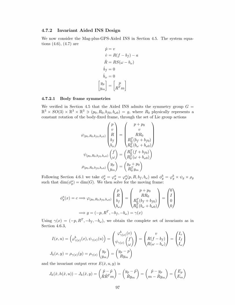
4.7.2 Invariant Aided INS Design
We now consider the Mag-plus-GPS-Aided INS in Section 4.5. The system equa-tions (4.6), (4.7) are
p = v
v = R(f − bf )− a
R = RS(ω − bω)
bf = 0
bω = 0[ypym
]=
[p
RTm
]
4.7.2.1 Body frame symmetries
We verified in Section 4.5 that the Aided INS admits the symmetry group G =R3 × SO(3) × R
3 × R3 ∋ (p0, R0, bf0, bω0) = g, where R0 physically represents a
constant rotation of the body-fixed frame, through the set of Lie group actions
ϕ(p0,R0,bf0,bω0)
pvRbfbω
=
p+ p0v
RR0
RT0 (bf + bf0)RT0 (bω + bω0)
ψ(p0,R0,bf0,bω0)
(fω
)=
(RT0 (f + bf0)RT0 (ω + bω0)
)
ρ(p0,R0,bf0,bω0)
(ypym
)=
(yp + p0RT0 ym
)
Following Section 4.6.1 we take φag = ϕag = ϕag(p,R, bf , bω) and φbg = ϕbg × ψg × ρgsuch that dim(φag) = dim(G). We then solve for the moving frame:
φag(x) = c =⇒ ϕ(p0,R0,bf0,bω0)
pRbfbω
=
p+ p0RR0
RT0 (bf + bf0)RT0 (bω + bω0)
=
0I00
=⇒ g = (−p,RT ,−bf ,−bω) = γ(x)
Using γ(x) = (−p,RT ,−bf ,−bω), we obtain the complete set of invariants as inSection 4.6.3,
I(x, u) =(ϕbγ(x)(x), ψγ(x)(u)
)=
ϕbγ(x)(v)
ψγ(x)
(fω
) =
vR(f − bf )R(ω − bω)
=
IvIfIω
Jh(x, y) = ργ(x)(y) = ργ(x)
(ypym
)=
(yp − pRym
)
and the invariant output error E(x, u, y) is
Jh(x, h(x, u))− Jh(x, y) =
(p− p
RRTm
)−(yp − p
Rym
)=
(p− yp
m− Rym
)=
(EpEm
)
97
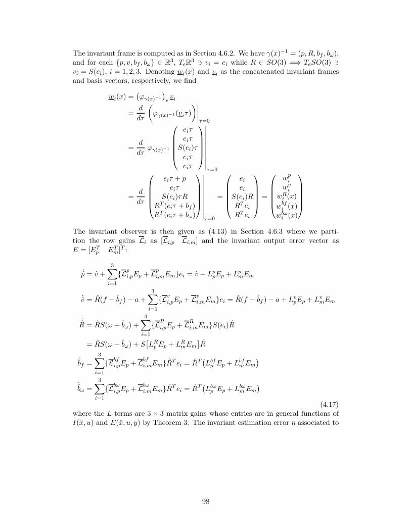
The invariant frame is computed as in Section 4.6.2. We have γ(x)−1 = (p,R, bf , bω),and for each p, v, bf , bω ∈ R
3, TeR3 ∋ vi = ei while R ∈ SO(3) =⇒ TeSO(3) ∋
vi = S(ei), i = 1, 2, 3. Denoting wi(x) and vi as the concatenated invariant framesand basis vectors, respectively, we find
wi(x) =(ϕγ(x)−1
)∗vi
=d
dτ
(ϕγ(x)−1(viτ)
)∣∣∣∣τ=0
=d
dτϕγ(x)−1
eiτeiτ
S(ei)τeiτeiτ
∣∣∣∣∣∣∣∣∣∣τ=0
=d
dτ
eiτ + peiτ
S(ei)τRRT (eiτ + bf )RT (eiτ + bω)
∣∣∣∣∣∣∣∣∣∣τ=0
=
eiei
S(ei)RRT eiRT ei
=
wpiwvi
wRi (x)
wbfi (x)wbωi (x)
The invariant observer is then given as (4.13) in Section 4.6.3 where we parti-tion the row gains Li as [Li,p Li,m] and the invariant output error vector asE = [ETp ETm]
T :
˙p = v +
3∑
i=1
Lpi,pEp + Lpi,mEmei = v + LppEp + LpmEm
˙v = R(f − bf )− a+
3∑
i=1
Lvi,pEp + Lvi,mEmei = R(f − bf )− a+ LvpEp + LvmEm
˙R = RS(ω − bω) +
3∑
i=1
LRi,pEp + LRi,mEmS(ei)R
= RS(ω − bω) + S[LRp Ep + LRmEm
]R
˙bf =
3∑
i=1
Lbfi,pEp + Lbfi,mEmRT ei = RT(Lbfp Ep + LbfmEm
)
˙bω =
3∑
i=1
Lbωi,pEp + Lbωi,mEmRT ei = RT(Lbωp Ep + LbωmEm
)
(4.17)where the L terms are 3 × 3 matrix gains whose entries are in general functions ofI(x, u) and E(x, u, y) by Theorem 3. The invariant estimation error η associated to
98

the above observer is calculated from (4.14)
η = ϕγ(x)(x)− ϕγ(x)(x)
=
p− pv
RRT
R(bf − bf )
R(bω − bω)
−
p− pv
RRT
R(bf − bf )R(bω − bω)
=
p− pv − v
RRT − I
R(bf − bf )
R(bω − bω)
=
ηpηv
ηR − Iηbfηbω
where as before we have taken ηR = RRT instead of RRT − I for convenience. Wewill work out the dynamics η below, which by Theorem 4 are guaranteed to dependon the system’s trajectories only through the invariants Iv, If and Iω found above.The invariant output error components can be expressed as
Ep = p− yp = p− p = ηp
Em = m− Rym = m− RRTm = m− ηRm
and we proceed to compute the individual η dynamics:
ηp = ˙p− p
= v + LppEp + LpmEm − v
= ηv + LppEp + LpmEm
ηv = ˙v − v
= R(f − bf )− a+ LvpEp + LvmEm −R(f − bf ) + a
= If + LvpEp + LvmEm −R(f − bf + bf − bf )
= If + LvpEp + LvmEm −RRT R(f − bf )−R(bf − bf )
= If + LvpEp + LvmEm − (ηR)T If − ηbf
ηR =˙RRT − RRT RRT
= RS(ω − bω)RT + S
[LRp Ep + LRmEm
]RRT − RRTRS(ω − bω)R
T
= RS(bω − bω)RT + S
[LRp Ep + LRmEm
]ηR
= −RRTRS(bω − bω)RT + S
[LRp Ep + LRmEm
]ηR
= −ηRS(ηbω) + S[LRp Ep + LRmEm
]ηR
99
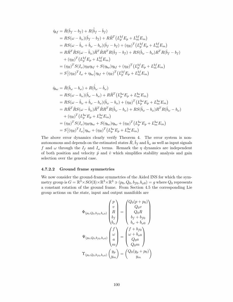
ηbf = R(bf − bf ) +R(˙bf − bf )
= RS(ω − bω)(bf − bf ) +RRT(Lbfp Ep + LbfmEm
)
= RS(ω − bω + bω − bω)(bf − bf ) + (ηR)T(Lbfp Ep + LbfmEm
)
= RRT RS(ω − bω)RT RRTR(bf − bf ) +RS(bω − bω)R
TR(bf − bf )
+ (ηR)T(Lbfp Ep + LbfmEm
)
= (ηR)TS(Iω)ηRηbf + S(ηbω)ηbf + (ηR)
T(Lbfp Ep + LbfmEm
)
= S[(ηR)
T Iω + ηbω]ηbf + (ηR)
T(Lbfp Ep + LbfmEm
)
ηbω = R(bω − bω) +R(˙bω − bω)
= RS(ω − bω)(bω − bω) +RRT(Lbωp Ep + LbωmEm
)
= RS(ω − bω + bω − bω)(bω − bω) + (ηR)T(Lbωp Ep + LbωmEm
)
= RRT RS(ω − bω)RT RRTR(bω − bω) +RS(bω − bω)R
TR(bω − bω)
+ (ηR)T(Lbωp Ep + LbωmEm
)
= (ηR)TS(Iω)ηRηbω + S(ηbω)ηbω + (ηR)
T(Lbωp Ep + LbωmEm
)
= S[(ηR)
T Iω]ηbω + (ηR)
T(Lbωp Ep + LbωmEm
)
The above error dynamics clearly verify Theorem 4. The error system is non-autonomous and depends on the estimated states R, bf and bω as well as input signalsf and ω through the If and Iω terms. Remark the η dynamics are independentof both position and velocity p and v which simplifies stability analysis and gainselection over the general case.
4.7.2.2 Ground frame symmetries
We now consider the ground-frame symmetries of the Aided INS for which the sym-metry group is G = R
3×SO(3)×R3×R
3 ∋ (p0, Q0, bf0, bω0) = g where Q0 representsa constant rotation of the ground frame. From Section 4.5 the corresponding Liegroup actions on the state, input and output manifolds are
Φ(p0,Q0,bf0,bω0)
pvRbfbω
=
Q0(p+ p0)Q0vQ0R
bf + bf0bω + bω0
Ψ(p0,Q0,bf0,bω0)
fωam
=
f + bf0ω + bω0Q0aQ0m
Υ(p0,Q0,bf0,bω0)
(ypym
)=
(Q0(yp + p0)
ym
)
100

We partition the Lie group action φg = Φg ×Ψg ×Υg as φag = Φag = Φag(p,R, bf , bω)
and φbg = Φbg ×Ψg ×Υg and solve φag(x) = c for the moving frame:
Φag
pRbfbω
=
Q0(p+ p0)Q0R
bf + bf0bω + bω0
=
0I00
=⇒ g = (−p,RT ,−bf ,−bω) = γ(x)
The complete set of invariants is then
I(x, u) =
(Φbγ(x)(x)
Ψγ(x)(u)
)=
Φb(−p,RT ,−bf ,−bω)
(v)
Ψ(−p,RT ,−bf ,−bω)
fωam
=
RTvf − bfω − bωRTaRTm
=
IvIfIωIaIm
Jh(x, y) = Υγ(x)(y) = Υ(−p,RT ,−bf ,−bω)
(ypym
)=
(RT (yp − p)
ym
)
The invariant output error is
E(x, u, y) = Jh(x, h(x, u))− Jh(x, y)
=
(RT (p− p)
RTm
)−(RT (yp − p)
ym
)=
(RT (p − yp)
RTm− ym
)=
(EpEm
)
For the invariant frame computation, we have γ(x)−1 = (p,R, bf , bω) and the samevi as in Section 4.7.2.1. We find
wi(x) =(Φγ(x)−1
)∗vi
=d
dτ
(Φγ(x)−1(viτ)
)∣∣∣∣τ=0
=d
dτΦγ(x)−1
eiτeiτ
S(ei)τeiτeiτ
∣∣∣∣∣∣∣∣∣∣τ=0
=d
dτ
R(eiτ + p)Reiτ
RS(ei)τeiτ + bfeiτ + bω
∣∣∣∣∣∣∣∣∣∣τ=0
=
ReiRei
RS(ei)eiei
=
wpi (x)wvi (x)wRi (x)
wbfiwbωi
101

The invariant observer is then
˙p = v +3∑
i=1
Lpi,pEp + Lpi,mEmRei = v + R(LppEp + LpmEm
)
˙v = R(f − bf )− a+3∑
i=1
Lvi,pEp + Lvi,mEmRei
= R(f − bf )− a+ R(LvpEp + LvmEm
)
˙R = RS(ω − bω) +
3∑
i=1
LRi,pEp + LRi,mEmRS(ei)
= RS(ω − bω) + RS[LRp Ep + LRmEm
]
˙bf =
3∑
i=1
Lbfi,pEp + Lbfi,mEmei = Lbfp Ep + LbfmEm
˙bω =
3∑
i=1
Lbωi,pEp + Lbωi,mEmei = Lbωp Ep + LbωmEm
(4.18)
where as in Section 4.7.2.1 the L terms are 3× 3 matrix gains whose entries are ingeneral functions of I(x, u) and E(x, u, y). The invariant estimation error η for thisobserver is
η = Φγ(x)(x)− Φγ(x)(x)
=
RT (p− p)RT v
RT R
bf − bfbω − bω
−
RT (p− p)RT vRTRbf − bfbω − bω
=
RT (p− p)RT (v − v)
RT R− I
bf − bfbω − bω
=
ηpηv
ηR − Iηbfηbω
The invariant output error E components are written as
Ep = RT (p− yp) = RTRRT (p− p) = (ηR)T ηp
Em = RTm− ym = RTm−RTm = Im −RT RRTm = Im − ηRIm
102

We now work out the η dynamics:
ηp = −RT RRT (p− p) +RT ( ˙p − p)
= −RTRS(ω − bω)RT (p− p) +RT
(v + R
(LppEp + LpmEm
)− v)
= −S(ω − bω + bω − bω)ηp + ηv +RT R(LppEp + LpmEm
)
= −S[Iω + ηbω
]ηp + ηv + ηR
(LppEp + LpmEm
)
ηv = −RT RRT (v − v) +RT ( ˙v − v)
= −RTRS(ω − bω)RT (v − v)
+RTR(f − bf )− a+ R
(LvpEp + LvmEm
)−R(f − bf ) + a
= −S(ω − bω + bω − bω)ηv + ηRIf + ηR(LvpEp + LvmEm
)− (f − bf + bf − bf )
= −S[Iω + ηbω
]ηv + ηRIf + ηR
(LvpEp + LvmEm
)− If − ηbf
ηR = −RT RRT R+RT˙R
= −RTRS(ω − bω)RT R+RT RS(ω − bω) +RT RS
[LRp Ep + LRmEm
]
= −S(ω − bω + bω − bω)ηR + ηRS(Iω) + ηRS[LRp Ep + LRmEm
]
= −S[Iω + ηbω
]ηR + ηRS(Iω) + ηRS
[LRp Ep + LRmEm
]
ηbf =˙bf − bf
= Lbfp Ep + LbfmEm
ηbω =˙bω − bω
= Lbωp Ep + LbωmEm
The ground-frame symmetry version of the invariant observer has properties similarto the body-frame symmetry version in Section 4.7.2.1: the estimation error dynam-ics η are a function of the system estimates via R, bf and bω as well as inputs f , ωbut independent of position and velocity p and v.
4.7.2.3 Combined symmetries
In Section 4.5 we also considered the combined symmetry case of rotating both thebody and ground frames. The corresponding Lie group actions were denoted by ξg,υg and g. Based on Section 4.7.1.3, we may expect this case to reduce to one ofthe previous results.
Take the Lie group action φg = ξg × υg × g; with the symmetry group G =R3 × SO(3) × SO(3) × R
3 × R3 ∋ (p0, Q0, R0, bf0, bω0) = g and state manifold
X = R3 × R
3 × SO(3) × R3 × R
3 ∋ (p, v,R, bf , bω) = g both of dimension 15, welogically partition φag = ξg, φ
bg = υg × g and (attempt to) solve for the moving
103

frame:
ξg
pvRbfbω
=
Q0(p+ p0)Q0v
Q0RR0
RT0 (bf + bf0)RT0 (bω + bω0)
=
00I00
We immediately see two problems:
• Q0v = 0 has no solution for Q0 ∈ SO(3) except in the trivial case of v = 0.In the more general case of Q0v = c, c ∈ R
3, a solution will exist only if‖v‖ = ‖c‖.
• Q0RR0 = I has a non-unique solution: Q0 = (RR0)T or alternatively R0 =
(Q0R)T .
We deal with this problem by a different choice of φag components, c.f. Section 4.7.1.3.We remove the ξg(v) component and replace it with υg(a) which provides a systemwhich can be solved for the moving frame:
φag
paRbfbω
=
Q0(p+ p0)Q0a
Q0RR0
RT0 (bf + bf0)RT0 (bω + bω0)
=
0aI00
=⇒ g = (−p, I,RT ,−bf ,−bω) = γ(x)
and the complete set of invariants is
φbγ(x)
vfωmypym
=
vR(f − bf )R(ω − bω)
myp − pRym
=
(I(x, u)Jh(x, y)
)
which are precisely the invariants in Section 4.7.2.1, such that the invariant observerfor the combined symmetries case will be identical to the earlier design. The invari-ant estimation error and its dynamics will also be identical to Section 4.7.2.1 dueto the Q0 = I term. While using the combined symmetries case is valid, it resultsin greater complexity and provides the same design as a simpler case. A combinedsymmetries version of invariant observer design was used in [92] for an Aided INSexample with different dynamics and outputs than (4.6) and (4.7).
4.8 Nonlinear Observer Gain Design
So far, we have not said anything about gain selection for stabilizing the observer.As mentioned in Section 4.6.3, there is no general systematic approach for choos-ing the nonlinear observer gains L. Using the invariant AHRS observer (4.15) withbody-frame symmetries in Section 4.7.1.1, we now show how a particular choice ofgains reduces it to the “explicit complementary filter with bias correction” in [88,
104

Thm. 5.1], for which almost global asymptotic stability [78]1 has been proven us-ing a Lyapunov analysis; this is the strongest result achievable since any systemwhose state manifold includes SO(3) cannot be globally asymptotically stable [20].Observer (4.15) is repeated here for convenience:
˙R = RS(ω − bω) + S
(LRa Ea + LRmEm
)R
˙bω = RT
(LωaEa + LωmEm
)
We make the following gain choices:
LRa = kP laS(a) LRm = kP lmS(m)
Lωa = −kI laS(a) Lωm = −kI lmS(m)(4.19)
where kP , kI , la, lm ∈ R are user-selected constants and a,m ∈ R3 are the ground-
frame gravity and magnetic field vectors used previously. This set of constant gainsobviously satisfies L = L(I,E) and so the observer is invariant. Remark that wehave reduced the tuning degrees of freedom from 4× 9 = 36 to 4.
Using the above gains and the invariant error definitions Ea = a − Rya, Em =m− Rym in (4.15) gives
˙R = RS(ω − bω) + S
(kP laS(a)(a − Rya) + kP lmS(m)(m− Rym)
)R
˙bω = RT
(− kI laS(a)(a − Rya)− kI lmS(m)(m− Rym)
)
since S(a)a = a× a = 0 and S(m)m = m×m = 0, we have
˙R = RS(ω − bω)− kPS
(laS(a)Rya + lmS(m)Rym
)R
˙bω = kIR
T(laS(a)Rya + lmS(m)Rym
)
Using RTS(v)R = S(RT v) =⇒ S(v)R = RS(RT v) from Section 2.2, we have
˙R = RS(ω − bω)− kP RS
(laR
TS(a)Rya + lmRTS(m)Rym
)
˙bω = kI
(laR
TS(a)Rya + lmRTS(m)Rym
)
We also have RTS(v)R = S(RT v) = S(yv) where v = a,m:
˙R = RS(ω − bω)− kP RS
(laS(ya)ya + lmS(ym)ym
)
˙bω = kI
(laS(ya)ya + lmS(ym)ym
)
And since S(yv)yv = yv × yv = −yv × yv we obtain
˙R = R
(S(ω − bω) + kPS
(laya × ya + lmym × ym
))
˙bω = −kI
(laya × ya + lmym × ym
),
1A system is almost globally asymptotically stable if all trajectories starting in an open densesubset of the state space asymptotically converge to a stable equilibrium; or equivalently, theset of initial conditions for which the trajectories do not converge form a set of zero Lebesguemeasure [103].
105

which is identical to [88, Eqn. (32)] modulo choice of notation.It is also possible to reduce the ground-frame symmetries invariant observer
(4.16),˙R = RS(ω − bω) + RS
(LRa Ea + LRmEm
)
˙bω = LωaEa + LωmEm,
to [88, Eqn. (32)] using the (different) set of gains
LRa = kP laS(RTa) LRm = kP lmS(R
Tm)
Lωa = −kI laS(RTa) Lωm = −kI lmS(RTm)(4.20)
where as before kP , kI , la, lm are constant scalars. Note that in Section 4.7.1.2,we computed Ia = RTa, Im = RTm and so the above gains respect the invariantobserver condition L = L(I,E). Using these gains and Ea = RTa − ya, Em =RTm− ym in (4.16) gives
˙R = RS(ω − bω) + RS
[kP laS(R
Ta)(RT a− ya) + kP lmS(RTm)(RTm− ym)
]
˙bω = −kI laS(RTa)(RTa− ya)− kI lmS(R
Tm)(RTm− ym)
using RTa = ya, RTm = ym, S(x)y = x× y and y × y = 0 we obtain
˙R = RS(ω − bω)− kP RS
(laya × ya + lmym × ym
)
˙bω = kI
(laya × ya + lmym × ym
)
and then from x× y = −y × x we have
˙R = R
(S(ω − bω) + kPS
(laya × ya + lmym × ym
))
˙bω = −kI
(laya × ya + lmym × ym
),
the observer [88, Eqn. (32)]. Remark the gain choices for L are different for the body-frame symmetries observer (4.15) and the ground-frame symmetries observer (4.16),but in both cases the observer in [88] is (a particular choice of) an invariant observer.
A nonlinear design for the gains of Aided INS observers (4.17), (4.18) remainsan open problem. Recent work in [31, 24] provides direct nonlinear gain designsfor a GPS-aided dead-reckoning system (c.f. [51, Ch. 9]) guaranteeing local, almostglobal or global stability depending on the level of assumptions made about thesystem’s state and inputs. Dead reckoning is a 2-dimensional aided navigationproblem and so it is reasonable to expect the analysis method can be extended toAided INS (4.6), (4.7) in Section 4.5, however no results have been obtained at thetime of writing. Another source of ideas are the direct nonlinear observer designsin [69, 118] for the velocity-aided inertial navigation example considered in [27].
4.9 Invariant Extended Kalman Filter
Although a direct nonlinear design for the observer gains L is the most elegant ap-proach, it is also difficult and non-systematic. In this Section we propose a method
106

of gain assignment based on the Extended Kalman Filter covered in Section 3.2.The Invariant EKF re-linearizes the invariant estimation error η dynamics (insteadof the system dynamics f(x, u) as in the conventional EKF) about the latest esti-mated state and computes optimal observer gains L for the resulting system. Thisprovides a fully systematic approach to obtaining the observer gains, which are alsoautomatically updated in the case of changing noise conditions due to the optimalityof the Kalman Filter. The obvious disadvantage is that the Invariant EKF guaran-tees only local stability whose region of attraction is difficult to analyze as discussedin Section 4.1.
Using an EKF to find the gains of an invariant observer was first proposed in [23]and applied to different examples in [29, 96]. The method in [23] was formulatedfor the class of systems where the Lie group G acts on itself by left or right transla-tion (c.f. Section 4.6.1) and required defining invariant noise terms which preservethe symmetry of the system. We adapt the method to apply to the general classof G-invariant systems defined in Section 4.3 and such that the noise terms canenter the dynamics naturally as part of the sensor models, c.f. Section 3.2.2. Themodified Invariant EKF can thus be applied to AHRS with body-frame symmetries(Section 4.4) and Aided INS (Section 4.5).
4.9.1 Invariant EKF Overview
We first review the continuous-time Kalman filter, e.g. [34, Chap. 7]. The filterapplies to LTV systems
x = A(t)x+B(t)w
y = C(t)x+D(t)v(4.21)
where w and v are the process and measurement Gaussian white noise vectors withcovariances Q = E〈wwT 〉, R = E〈vvT 〉, respectively, and zero cross-correlation:E〈wvT 〉 = 0. The Kalman filter for (4.21) is
˙x = Ax+K(y − Cx)
K = PCT (DRDT )−1
P = AP + PAT − PCT (DRDT )−1CP +BQBT ,
(4.22)
a linear optimal observer designed to minimize the covariance of the estimation errore = x− x, specifically min
(trace(E〈e eT 〉)
). From (4.22) and (4.21), the estimation
error dynamics are
e = ˙x− x
= Ax+K (Cx+Dv − Cx)−Ax−Bw
= (A−KC)(x− x)−Bw +KDv
e = (A−KC)e−Bw +KDv (4.23)
The method of the Invariant EKF is as follows: introduce the sensor noise modelsu = u + w, y = y + v from Section 3.2.2 into the nominal system dynamics andcorresponding invariant observer as
x = f(x, u) = f(x, u− w) (4.24a)
˙x = F (x, u, y) = F (x, u, y + v) (4.24b)
107

Using the existing invariant estimation error η (4.14) for this system, compute(d/dt)η using terms (4.24) which yields the nonlinear dynamics
d
dtη = Ξ(η, x, u, w, v), (4.25)
a more complicated system than in Theorem 4 due to the use of (4.24); note Ξnecessarily reduces to Υ(η, I(x, u)) when w = v = 0. Let η denote zero estimationerror, e.g. ηR = I and ηω = 0 for the Invariant AHRS observer in Section 4.7.1, anddefine δη := η − η. Due to the form of the invariant estimation error (4.14)
η = ϕγ(x)(x)− ϕγ(x)(x)
when computing Ξ, the terms x (4.24a) and ˙x (4.24b) which respectively containw and v,K (K denotes the matrix of observer gains L) do not appear together inproduct terms. Thus linearizing (4.25) about η = η, w = 0 and v = 0 leads to thesame form as (4.23),
δη = (A−KC)δη −Bw +KDv (4.26)
from which we can read off the (A,B,C,D) and K matrices and use (4.22) tocompute the observer gains L which make up the matrix K. Remark that theentries of the A,B,C,D matrices will in general be functions of (x, u), so as statedin Section 4.9 we are re-linearizing the invariant estimation error dynamics aboutthe latest state estimate.
4.9.2 Invariant AHRS EKF design
As mentioned in Section 4.2, we model the AHRS bias dynamics using the Wienerprocess model b = ν. We also employ the rate gyro sensor model ω = ω + bω + νωand accelerometer and magnetometer output models y = y + ν from Section 3.2.2.Under these noise models the dynamics of (4.1) become (4.24a)
R = RS(ω − bω − νω)
bω = νbω(4.27)
where w = [νω νbω ]T is the process noise vector. The system outputs with noise
are [yaym
]=
[RTa+ νaRTm+ νm
](4.28)
with v = [νa νm]T the measurement noise vector; as discussed in Section 4.2 we
assume the accelerometer measures the gravity vector and the magnetometer readinghas been compensated.
4.9.2.1 Body frame symmetries
The nominal invariant observer is available from Section 4.7.1.1 as (4.15). Using thenoise models in Section 4.9.2 we obtain (4.24b)
˙R = RS(ω − bω) + S
(LRa Ea + LRmEm
)R
˙bω = RT
(Lωa Ea + LωmEm
) (4.29)
108

where ω is the measured rate gyro signal. The Ea, Em invariant output errorsin (4.29) and I(x, u) invariants used below are also available from Section 4.7.1.1:
(EaEm
)=
(a− Ryam− Rym
), I(x, u) = R(ω − bω), (4.30)
where ya, ym are the output measurements and I(x, u) is known and will appearbelow. The invariant error η (4.14) is a function of x and x only and remainsunchanged from Section 4.7.1.1, i.e. ηR = RRT , ηω = R(bω − bω). As explainedin Section 4.9.1, computing (d/dt)η using (4.27) and (4.29) will cause the processnoise vector w = [νω νbω ]
T to appear along with the measurement noise vectorv = [νa νm]
T embedded in E. Starting with ηR we directly compute
ηR =˙RRT + R
d
dt(RT )
= RS(ω − bω)RT + S
(LRa Ea + LRmEm
)RRT + R
(−RTRS(ω − bω − νω)R
T)
= RS(bω − bω)RT + S
(LRa Ea + LRmEm
)RRT + RS(νω)R
T
= RRTRS(bω − bω)RT + S
(LRa Ea + LRmEm
)RRT + RS(νω)R
T RRT
= RRTS[R(bω − bω)
]+ S
(LRa Ea + LRmEm
)RRT + S(Rνω)RR
T
ηR = ηRS(−ηω) + S(LRa Ea + LRmEm
)ηR + S(Rνω)ηR
and for ηω we have
ηω = R(bω − bω) +R(˙bω − bω)
= RS(ω − bω − νω)(bω − bω) +RRT(Lωa Ea + LωmEm
)− νbω
= RS(ω − bω + bω − bω)(bω − bω) +RRT(Lωa Ea + LωmEm
)
−Rνbω −RS(νω)(bω − bω)
= RS(ω − bω + bω − bω)RTR(bω − bω) +RRT
(Lωa Ea + LωmEm
)
−Rνbω +RS(bω − bω)νω
=RS(ω − bω)R
T +RS(bω − bω)RTR(bω − bω) + (RRT )T
(Lωa Ea + LωmEm
)
−RRT Rνbω +RS(bω − bω)RTRRT Rνω
=RRT RS(ω − bω)R
T RRT + S[R(bω − bω)
]R(bω − bω)
+ (RRT )T(Lωa Ea + LωmEm
)− (RRT )T Rνbω + S
[R(bω − bω)
](RRT )T Rνω
= (RRT )TS[R(ω − bω)
]RRT ηω + (ηR)
T(Lωa Ea + LωmEm
)
− (ηR)T Rνbω + S [ηω] (ηR)
T Rνω
ηω = S[(ηR)
T I(x, u)]ηω + (ηR)
T(Lωa Ea + LωmEm
)− (ηR)
T Rνbω + S [ηω] (ηR)T Rνω
where the E terms are written as
(EaEm
)=
(a− Ryam− Rym
)=
(a− R(RTa+ νa)
m− R(RTm+ νm)
)=
(a− ηRa− Rνam− ηRm− Rνm
)
109

which contains the measurement noise vector v = [νa νm]T . Remark I(x, u) ap-
pears in the ηω term above, and as expected setting w = v = 0 reduces bothdynamics to the form (d/dt)η = Υ(η, I(x, u)) guaranteed by Theorem 4.
We now linearize the above ηR and ηω dynamics about ηR = I, ηω = 0 and ν = 0to obtain system (4.26) with states δη = η − η. The Ev, v ∈ a,m terms become
δEv = Ev − Ev = v − ηRv − Rνv − v + ηRv + Rνv = −δηRv − Rνv
Ev = v − ηRv − Rνv = v − v = 0.
Linearizing ηR we obtain
δηR = ηR − ˙ηR
= ηRS(−ηω) + S(LRa Ea + LRmEm
)ηR + S(Rνω)ηR
− ηRS(−ηω)− S(LRa Ea − LRmEm
)ηR − S(Rνω)ηR
= (δηR + ηR)S(−δηω − ηω) + S[LRa (δEa + Ea) + LRm(δEm + Em)
](δηR + ηR)
+ S[R(δνω + νω)
](δηR + ηR)− ηRS(−ηω)− S
(LRa Ea − LRmEm
)ηR
− S(Rνω)ηR
= (δηR + ηR)S(−δηω) + S[LRa δEa + LRmδEm
](δηR + ηR)
+ S[R(δνω)
](δηR + ηR)
= ηRS(−δηω) + S[LRa δEa + LRmδEm
]ηR + S
[R(δνω)
]ηR
= S(−δηω) + S[LRa (−δηRa− Rνa) + LRm(−δηRm− Rνm)
]+ S[Rνω]
where we have dropped quadratic terms in δ on the second-last line in order toobtain a linear equation. For ηω we obtain the linearization
δηω = ηω − ˙ηω
= S[(ηR)
T I(x, u)]ηω + (ηR)
T(Lωa Ea + LωmEm
)− (ηR)
T Rνbω + S[ηω](ηR)T Rνω
− S[(ηR)
T I(x, u)]ηω − (ηR)
T(Lωa Ea − LωmEm
)+ (ηR)
T Rνbω
− S[ηω](ηR)T Rνω
= S[(δηR + ηR)
T I(x, u)](δηω + ηω) + (δηR + ηR)
T(Lωa (δEa + Ea)
+ Lωm(δEm + Em))− (δηR + ηR)
T R(δνbω + νbω)
+ S[δηω + ηω](δηR + ηR)T R(δνω + νω)
= S[(ηR)
T I(x, u)]δηω + (ηR)
T(Lωa δEa + LωmδEm
)− (ηR)
T Rδνbω
= S[I(x, u)]δηω + Lωa (−δηRa− Rνa) + Lωm(−δηRm− Rνm)− Rνbω
where we have again dropped all quadratics in δ on the second-last line above. Wefurther simplify the above expressions by re-expressing δηR = ηR − ηR = RRT − Iusing the same technique as in Section 3.2.5: take the ground-frame rotationalkinematics (2.3) (d/dt)R = S(ω)R and define ω = dγ/dt. The kinematics getwritten as dR/dt = S(dγ/dt)R =⇒ dR = S(dγ)R. For the linearization pointηR = I, we can write dR ≈ R−R and dγ = γ − γ, and so R−R ≈ S(γ − γ)R =⇒RRT − I = S(γ − γ) =⇒ δηR = S(δγ), where δγ gets used to represent attitudeerror in the linearized system in place of δηR.
110

Using δηR = S(δγ) in the ηR and ηω expressions above, we obtain
S(δγ) = S(−δηω) + S[LRa (−S(δγ)a − Rνa) + LRm(−S(δγ)m − Rνm)
]+ S[Rνω]
S(δγ) = S[− δηω + LRa (S(a)δγ − Rνa) + LRm(S(m)δγ − Rνm) + Rνω
]
δγ = −δηω +[LRa S(a) + LRmS(m)
]δγ − LRa Rνa − LRmRνm + Rνω
for δηR, and for δηω we have
δηω = S[I(x, u)]δηω + Lωa (−S(δγ)a − Rνa) + Lωm(−S(δγ)m − Rνm)− Rνbω
= S[I(x, u)]δηω + Lωa (S(a)δγ − Rνa) + Lωm(S(m)δγ − Rνm)− Rνbω
δηω = S[I(x, u)]δηω +[LωaS(a) + LωmS(m)
]δγ − Lωa Rνa − LωmRνm − Rνbω
The δγ and δηω expressions are rewritten as (4.26)
[δγδηω
]=
[0 −I0 S[I(x, u)]
]
︸ ︷︷ ︸A
[δγδηω
]−[LRa LRmLωa Lωm
]
︸ ︷︷ ︸K
[−S(a) 0−S(m) 0
]
︸ ︷︷ ︸C
[δγδηω
]
−[−R 0
0 R
]
︸ ︷︷ ︸B
[νωνbω
]
︸ ︷︷ ︸w
+
[LRa LRmLωa Lωm
]
︸ ︷︷ ︸K
[−R 0
0 −R
]
︸ ︷︷ ︸D
[νaνm
]
︸ ︷︷ ︸v
(4.31)
Using the set of matrices (A,B,C,D) along with the (identified) noise covariancesQ = E〈wwT 〉, R = E〈vvT 〉 we use (4.22) to calculate K and use the resulting gainsL in the invariant observer (4.29) resp. (4.15).
4.9.2.2 Ground frame symmetries
We also design an Invariant EKF for the AHRS ground-frame symmetry case coveredin Section 4.7.1.2. Under additive noise, the system dynamics and outputs are stillgiven by (4.27), (4.28)
R = RS(ω − bω − νω)
bω = νbω[yaym
]=
[RTa+ νaRTm+ νm
]
while the observer (4.16) becomes
˙R = RS(ω − bω) + RS
(LRa Ea + LRmEm
)
˙bω = Lωa Ea + LωmEm
where Ea = RTa− ya, Em = RTm− ym. The invariant estimation errors ηR = RT R,ηω = bω − bω are unchanged from Section 4.7.1.2, and we compute their dynamics
111

below:
ηR = −RT RRT R+RT˙R
= −RTRS(ω − bω − νω)RT R+RT RS(ω − bω) +RT RS
(LRa Ea + LRmEm
)
= ηRS(Iω)− S(Iω)ηR − S(ηω)ηR + ηRS(LRa Ea + LRmEm
)+ S(νω)ηR
ηω =˙bω − bω
= Lωa Ea + LωmEm − νbω
where Iω = ω− bω as well as Ia = RTa, Im = RTm are the invariants of the system,the latter two appearing in the invariant output errors:
Ea = RTa− ya = RTa−RTa− νa = Ia −RT RRTa− νa = Ia − ηRIa − νa
Em = RTm− ym = RTm−RTm− νm = Im −RT RRTm− νm = Im − ηRIm − νm
Next, we linearize the above η dynamics about ηR = I, ηω = 0 and ν = 0. The Eterms will become
δEa = Ea − Ea = Ia − ηRIa − νa − Ia + ηRIa + νa = −δηRIa − νa
δEm = Em − Em = Im − ηRIm − νm − Im + ηRIm + νm = −δηRIm − νm
where Ea = Em = 0. Using δηR = S(δγ) as in Section 4.9.2.1, we have
δEa = −S(δγ)Ia − νa = S(Ia)δγ − νa
δEm = −S(δγ)Im − νm = S(Im)δγ − νm
Finally, we calculate the linearized δη dynamics as
δηR = ηR − ˙ηR
= ηRS(Iω)− S(Iω)ηR − S(ηω)ηR + ηRS(LRa Ea + LRmEm
)+ S(νω)ηR − 0
= (δηR + ηR)S(Iω)− S(Iω)(δηR + ηR)− S[δηω + ηω](δηR + ηR)
+ (δηR + ηR)S(LRa (δEa + Ea) + LRm(δEm + Em)
)
+ S[δνω + νω](δηR + ηR)
= δηRS(Iω)− S(Iω)δηR − S(δηω)ηR + ηRS(LRa δEa + LRmδEm
)+ S(δνω)ηR
S(δγ) = S(δγ)S(Iω)− S(Iω)S(δγ) − S(δηω) + S(LRa δEa + LRmδEm
)+ S(νω)
δγ = δγ × Iω − δηω + LRa δEa + LRmδEm + νω
= −S(Iω)δγ − δηω + LRa(S(Ia)δγ − νa
)+ LRm
(S(Im)δγ − νm
)+ νω
andδηω = ηω − ˙ηω
= Lωa Ea + LωmEm − νbω − Lωa Ea − LωmEm + νbω
= Lωa δEa + LωmδEm − νbω
= Lωa(S(Ia)δγ − νa
)+ Lωm
(S(Im)δγ − νm
)− νbω
112

which is rewritten in form (4.26) as
[δγδηω
]=
[−S[ω − bω] −I
0 0
]
︸ ︷︷ ︸A
[δγδηω
]−[LRa LRmLωa Lωm
]
︸ ︷︷ ︸K
[−S[RTa] 0
−S[RTm] 0
]
︸ ︷︷ ︸C
[δγδηω
]
−[−I 00 I
]
︸ ︷︷ ︸B
[νωνbω
]
︸ ︷︷ ︸w
+
[LRa LRmLωa Lωm
]
︸ ︷︷ ︸K
[−I 00 −I
]
︸ ︷︷ ︸D
[νaνm
]
︸ ︷︷ ︸v
(4.32)
Which provides the set (A,B,C,D) used in (4.22) to calculate the gains L of theinvariant observer (4.16).
4.9.3 Invariant Aided INS EKF design
In order to assign the gains L to the Aided INS observers designed in Sections 4.7.2.1and 4.7.2.2, we use the Invariant EKF methodology of Section 4.9.1. We considerboth the body-frame and ground-frame symmetries versions below. Using the ac-celerometer and rate gyro sensor models (3.4) f = f + bf + νf , ω = ω + bω + νωfrom Section 3.2.2 along with a Wiener process model for the bias dynamics b = νas mentioned in Section 4.5, the Aided INS dynamics (4.6) become (4.24a)
p = v
v = R(f − bf − νf )− a
R = RS(ω − bω − νω)
bf = νbf
bω = νbω
(4.33)
with process noise vector w = [νf νω νbf νbω]T . The nominal output equa-
tions (4.7) become [ypym
]=
[p+ νp
RTm+ νm
](4.34)
where v = [νp νm]T is the measurement noise vector. As discussed in Section (4.5)
we assume the Navigation to ECEF rotation matrix RNE and location of navigationframe roE have been found such that the vehicle’s navigation frame position p isdirectly measurable. The vector m is the navigation frame magnetic field vector,c.f. Section 2.8, and ym is assumed compensated such that νm := νcm, c.f. Sec-tion 3.2.2.
113

4.9.3.1 Body frame symmetries
From Section 4.7.2.1, the invariant observer (4.17) with noise models from Sec-tion 4.9.3 takes the form (4.24b)
˙p = v + LppEp + LpmEm
˙v = R(f − bf )− a+ LvpEp + LvmEm
˙R = RS(ω − bω) + S
[LRp Ep + LRmEm
]R
˙bf = RT
(Lbfp Ep + Lbfm Em
)
˙bω = RT
(Lbωp Ep + Lbωm Em
)
where Ep = p − yp and Em = m − Rym. The invariant estimation errors η remainunchanged, and the dynamics η are expected to contain the invariants Iv = v,If = R(f − bf ) and Iω = R(ω − bω). By direct computation:
ηp = ˙p− p
= v + LppEp + LpmEm − v
= ηv + LppEp + LpmEm
ηv = ˙v − v
= R(f − bf )− a+ LvpEp + LvmEm −R(f − bf − νf ) + a
= If + LvpEp + LvmEm − (ηR)T If − ηbf +Rνf
= If + LvpEp + LvmEm − (ηR)T If − ηbf + (ηR)
T Rνf
ηR =˙RRT − RRT RRT
= RS(ω − bω)RT + S
[LRp Ep + LRmEm
]RRT − RRTRS(ω − bω − νω)R
T
= −ηRS(ηbω) + S[LRp Ep + LRmEm
]ηR + RS(νω)R
T
= −ηRS(ηbω) + S[LRp Ep + LRmEm
]ηR + RS(νω)R
T RRT
= −ηRS(ηbω) + S[LRp Ep + LRmEm
]ηR + S
[Rνω
]ηR
114

ηbf = R(bf − bf ) +R(˙bf − bf )
= RS(ω − bω − νω)(bf − bf ) +RRT(Lbfp Ep + Lbfm Em
)−Rνbf
= S[(ηR)
T Iω + ηbω]ηbf + (ηR)
T(Lbfp Ep + Lbfm Em
)−RS(νω)(bf − bf )−Rνbf
= S[(ηR)
T Iω + ηbω]ηbf + (ηR)
T(Lbfp Ep + Lbfm Em
)+RS[bf − bf ]νω −Rνbf
= S[(ηR)
T Iω + ηbω]ηbf + (ηR)
T(Lbfp Ep + Lbfm Em
)+RS[bf − bf ]R
TRRT Rνω
−RRT Rνbf
= S[(ηR)
T Iω + ηbω]ηbf + (ηR)
T(Lbfp Ep + Lbfm Em
)+ S[ηbf ](ηR)
T Rνω
− (ηR)T Rνbf
ηbω = R(bω − bω) +R(˙bω − bω)
= RS(ω − bω − νω)(bω − bω) +RRT(Lbωp Ep + Lbωm Em
)−Rνbω
= S[(ηR)
T Iω]ηbω + (ηR)
T(Lbωp Ep + Lbωm Em
)−RS(νω)(bω − bω)−Rνbω
= S[(ηR)
T Iω]ηbω + (ηR)
T(Lbωp Ep + Lbωm Em
)+RS[bω − bω]νω −Rνbω
= S[(ηR)
T Iω]ηbω + (ηR)
T(Lbωp Ep + Lbωm Em
)+RS[bω − bω]R
TRRT Rνω
−RRT Rνbω
= S[(ηR)
T Iω]ηbω + (ηR)
T(Lbωp Ep + Lbωm Em
)+ S[ηbω](ηR)
T Rνω − (ηR)T Rνbω
where we have
Ep = p− yp = p− p− νp = ηp − νp
Em = m− Rym = m− RRTm− Rνm = m− ηRm− Rνm
We now linearize the error dynamics above about η = 0 (ηR = I) and ν = 0. Theinvariant output error terms become
δEp = Ep − Ep = ηp − νp − ηp + νp = δηp − νp
δEm = Em − Em
= m− ηRm− Rνm −m+ ηRm+ Rνm = −δηRm− Rνm = S(m)δγ − Rνm
115

where we have used δηR = S(δγ) with δγ = γ − γ as explained in Section 4.9.2.1.
Remark that Ep = Em = 0. We now proceed to calculate the linearizations:
δηp = ηp − ˙ηp
= ηv + LppEp + LpmEm − ηv − LppEp − LpmEm
= δηv + LppδEp + LpmδEm
= δηv + Lpp(δηp − νp
)+ Lpm
(S(m)δγ − Rνm
)
δηv = ηv − ˙ηv
= If + LvpEp + LvmEm − (ηR)T If − ηbf + (ηR)
T Rνf
− If − LvpEp − LvmEm + (ηR)T If + ηbf − (ηR)
T Rνf
= LvpδEp + LvmδEm − (δηR)T If − δηbf + (δηR + ηR)
T R(δνf + νf )
= LvpδEp + LvmδEm −(S(δγ)
)TIf − δηbf + (ηR)
T Rδνf
= Lvp(δηp − νp
)+ Lvm
(S(m)δγ − Rνm
)− S(If )δγ − δηbf + Rνf
δηR = ηR − ˙ηR
= −ηRS(ηbω) + S[LRp Ep + LRmEm
]ηR + S(Rνω)ηR − 0
= −(δηR + ηR
)S[δηbω + ηbω
]+ S
[LRp(δEp + Ep
)
+ LRm(δEm + Em
)](δηR + ηR
)+ S
[R(δνω + νω
)](δηR + ηR
)
δηR = −ηRS(δηbω) + S[LRp δEp + LRmδEm
]ηR + S
[Rδνω
]ηR
S(δγ) = S(−δηbω) + S[LRp(δηp − νp
)+ LRm
(S(m)δγ − Rνm
)]+ S
[Rνω
]
δγ = −δηbω + LRp(δηp − νp
)+ LRm
(S(m)δγ − Rνm
)+ Rνω
116

δηbf = ηbf − ˙ηbf
= S[(ηR)
T Iω + ηbω]ηbf + (ηR)
T(Lbfp Ep + Lbfm Em
)
+ S[ηbf ](ηR)T Rνω − (ηR)
T Rνbf − 0
= S[(δηR + ηR
)TIω +
(δηbω + ηbω
)](δηbf + ηbf
)
+(δηR + ηR
)T(Lbfp(δEp + Ep
)+ Lbfm
(δEm + Em
))
+ S[δηbf + ηbf
](δηR + ηR
)TR(δνω + νω
)−(δηR + ηR
)TR(δνbf + νbf
)
= S[(ηR)TIω]δηbf +
(ηR)T(
Lbfp δEp + Lbfm δEm
)
+ S[δηbf
](ηR)TRδνω −
(ηR)TRδνbf
= S[Iω]δηbf + Lbfp
(δηp − νp
)+ Lbfm
(S(m)δγ − Rνm
)− Rνbf
δηbω = ηbω − ˙ηbω
= S[(ηR)
T Iω]ηbω + (ηR)
T(Lbωp Ep + Lbωm Em
)
+ S[ηbω](ηR)T Rνω − (ηR)
T Rνbω − 0
= S[(δηR + ηR
)TIω](δηbω + ηbω
)
+(δηR + ηR
)T(Lbωp(δEp + Ep
)+ Lbωm
(δEm + Em
))
+ S[δηbω + ηbω
](δηR + ηR
)TR(δνω + νω
)−(δηR + ηR
)TR(δνbω + νbω
)
= S[(ηR)TIω]δηbω +
(ηR)T(
Lbωp δEp + Lbωm δEm
)
+ S[δηbω
](ηR)TRδνω −
(ηR)TRδνbω
= S[Iω]δηbω + Lbωp
(δηp − νp
)+ Lbωm
(S(m)δγ − Rνm
)− Rνbω
117

The preceding are rewritten in the form (4.26):
δηpδηvδγδηbfδηbω
=
0 I 0 0 0
0 0 −S[If ] −I 00 0 0 0 −I0 0 0 S[Iω] 0
0 0 0 0 S[Iω]
︸ ︷︷ ︸A
δηpδηvδγδηbfδηbω
−
Lpp LpmLvp LvmLRp LRmLbfp LbfmLbωp Lbωm
︸ ︷︷ ︸K
[−I 0 0 0 00 0 −S(m) 0 0
]
︸ ︷︷ ︸C
δηpδηvδγδηbfδηbω
−
0 0 0 0
−R 0 0 0
0 −R 0 0
0 0 R 0
0 0 0 R
︸ ︷︷ ︸B
νfνωνbfνbω
︸ ︷︷ ︸w
+
Lpp LpmLvp LvmLRp LRmLbfp LbfmLbωp Lbωm
︸ ︷︷ ︸K
[−I 0
0 −R
]
︸ ︷︷ ︸D
[νpνm
]
︸ ︷︷ ︸v
which provides the required (A,B,C,D) matrices to compute K via (4.22) givingthe gains L of observer (4.17).
4.9.3.2 Ground frame symmetries
From Section 4.7.2.2, the invariant observer (4.18) with noise models from Sec-tion 4.9.3 takes the form (4.24b)
˙p = v + R(LppEp + LpmEm
)
˙v = R(f − bf )− a+ R(LvpEp + LvmEm
)
˙R = RS(ω − bω) + RS
[LRp Ep + LRmEm
]
˙bf = Lbfp Ep + Lbfm Em
˙bω = Lbωp Ep + Lbωm Em
118

As before the η expressions are unchanged by the addition of noise. We directlywork out their dynamics below:
ηp = −RT RRT (p− p) +RT ( ˙p − p)
= −RTRS(ω − bω − νω)RT (p− p) +RT
(v + R
(LppEp + LpmEm
)− v)
= −S[Iω + ηbω
]ηp + ηv + ηR
(LppEp + LpmEm
)+ S(νω)R
T (p − p)
= −S[Iω + ηbω
]ηp + ηv + ηR
(LppEp + LpmEm
)− S(ηp)νω
ηv = −RT RRT (v − v) +RT ( ˙v − v)
= −RTRS(ω − bω − νω)RT (v − v)
+RTR(f − bf )− a+ R
(LvpEp + LvmEm
)−R(f − bf − νf ) + a
= −S[Iω + ηbω
]ηv + ηRIf + ηR
(LvpEp + LvmEm
)
− If − ηbf + S(νω)RT (v − v) + νf
= −S[Iω + ηbω
]ηv + ηRIf + ηR
(LvpEp + LvmEm
)− If − ηbf − S(ηv)νω + νf
ηR = −RT RRT R+RT˙R
= −RTRS(ω − bω − νω)RT R+RT RS(ω − bω) +RT RS
[LRp Ep + LRmEm
]
= −S[Iω + ηbω
]ηR + ηRS(Iω) + ηRS
[LRp Ep + LRmEm
]+ S(νω)ηR
ηbf =˙bf − bf
= Lbfp Ep + Lbfm Em − νbf
ηbω =˙bω − bω
= Lbωp Ep + Lbωm Em − νbω
where Iω = ω− bω, If = f − bf as well as Im = RTm which appears in the invariantoutput errors:
Ep = RT (p− yp) = RT (p − p− νp) = RTRRT (p− p)− RT νp = (ηR)T ηp − RT νp
Em = RTm− ym = RTm−RTm− νm = Im −RT RRTm− νm = Im − ηRIm − νm
We linearize the system about η = 0 (ηR = I), ν = 0. We have
δEp = Ep − Ep
= (ηR)T ηp − RTνp − (ηR)
T ηp + RT νp
= (δηR + ηR)T (δηp + ηp)− RT νp
= (ηR)T δηp − RT νp = δηp − RTνp
δEm = Em − Em
= Im − ηRIm − νm − Im + ηRIm + νm
= −(δηR)Im − νm = −S(δγ)Im − νm = S(Im)δγ − νm
119
and for the invariant estimation dynamics
δηp = ηp − ˙ηp
= −S[Iω + ηbω
]ηp + ηv + ηR
(LppEp + LpmEm
)− S(ηp)νω − 0
= −S[Iω + δηbω + ηbω
](δηp + ηp
)+ δηv + ηv
+(δηR + ηR
)(Lpp(δEp + Ep
)+ Lpm
(δEm + Em
))
− S[δηp + ηp
](δνω + νω
)
= −S(Iω)δηp + δηv + ηR
(LppδEp + LpmδEm
)
= −S(Iω)δηp + δηv + Lpp(δηp − RTνp
)+ Lpm
(S(Im)δγ − νm
)
δηv = ηv − ˙ηv
= −S[Iω + ηbω
]ηv + ηRIf + ηR
(LvpEp + LvmEm
)− If − ηbf − S(ηv)νω + νf
+ S[Iω + ηbω
]ηv − ηRIf − ηR
(LvpEp + LvmEm
)+ If + ηbf + S(ηv)νω − νf
= −S(Iω)δηv − S[δηbω + ηbω
](δηv + ηv
)+ δηRIf
+(δηR + ηR
)(Lvp(δEp + Ep
)+ Lvm
(δEm + Em
))
− δηbf − S[δηv + ηv
](δνω + νω
)+ νf
= −S(Iω)δηv + S(δγ)If + ηR(LvpδEp + LvmδEm
)− δηbf + νf
= −S(Iω)δηv − S(If )δγ + Lvp(δηp − RT νp
)+ Lvm
(S(Im)δγ − νm
)− δηbf + νf
δηR = ηR − ˙ηR
= −S[Iω + ηbω
]ηR + ηRS(Iω) + ηRS
[LRp Ep + LRmEm
]+ S(νω)ηR
+ S[Iω + ηbω
]ηR − ηRS(Iω)− ηRS
[LRp Ep + LRmEm
]− S(νω)ηR
= −S(Iω)δηR − S[δηbω + ηbω
](δηR + ηR
)+ δηRS(Iω)
+(δηR + ηR
)S[LRp(δEp + Ep
)+ LRm
(δEm + Em
)]
+ S[δνω + νω
](δηR + ηR
)
δηR = δηRS(Iω)− S(Iω)δηR − S[δηbω
]ηR + ηRS
[LRp δEp + LRmδEm
]+ S
[δνω]ηR
S(δγ) = S(δγ)S(Iω)− S(Iω)S(δγ) − S[δηbω
]+ S
[LRp δEp + LRmδEm
]+ S
[νω]
δγ = δγ × Iω − δηbω + LRp δEp + LRmδEm + νω
= −S(Iω)δγ − δηbω + LRp(δηp − RTνp
)+ LRm
(S(Im)δγ − νm
)+ νω
120

δηbf = ηbf − ˙ηbf
= Lbfp Ep + Lbfm Em − νbf − Lbfp Ep − Lbfm Em + νbf
= Lbfp(δηp − RT νp
)+ Lbfm
(S(Im)δγ − νm
)− νbf
δηbω = ηbω − ˙ηbω
= Lbωp Ep + Lbωm Em − νbω − Lbωp Ep − Lbωm Em + νbω
= Lbωp(δηp − RT νp
)+ Lbωm
(S(Im)δγ − νm
)− νbω
We then rearrange the above expressions into form (4.26):
δηpδηvδγδηbfδηbω
=
−S(Iω) I 0 0 0
0 −S(Iω) −S(If ) −I 0
0 0 −S(Iω) 0 −I0 0 0 0 00 0 0 0 0
︸ ︷︷ ︸A
δηpδηvδγδηbfδηbω
−
Lpp LpmLvp LvmLRp LRmLbfp LbfmLbωp Lbωm
︸ ︷︷ ︸K
[−I 0 0 0 00 0 −S(Im) 0 0
]
︸ ︷︷ ︸C
δηpδηvδγδηbfδηbω
−
0 0 0 0−I 0 0 00 −I 0 00 0 I 00 0 0 I
︸ ︷︷ ︸B
νfνωνbfνbω
︸ ︷︷ ︸w
+
Lpp LpmLvp LvmLRp LRmLbfp LbfmLbωp Lbωm
︸ ︷︷ ︸K
[−RT 00 −I
]
︸ ︷︷ ︸D
[νpνm
]
︸ ︷︷ ︸v
giving the set of (A,B,C,D) matrices used with (4.22) to compute K resp. the gainsL of observer (4.18).
4.10 Invariant AHRS testing
4.10.1 Implementation Details
The invariant AHRS observers were designed in Section 4.7.1 and will be summarizedbelow. We numerically implement the equations using the modified Euler method,e.g. [35, p. 280]: for x = F (x, t), x(t0) = x0, the approximated states wi = x(ti),ti = t0 + iT with T representing the step size are calculated by
w0 = x0
wi+1 = wi +T
2
(F (ti, wi) + F (ti+1, wi + TF (ti, wi))
)i = 0, 1, 2, . . .
As in Section 3.2.1, we employ a complementary filter topology: the system dynam-ics part of the observer f(x, u) is integrated at the IMU sampling period TIMU to
121
produce rough state estimates x, which are periodically updated using aiding mea-surements ya, ym resp. Ea, Em and observer gains L at the user-selectable periodTAid ≥ TIMU. The terms L are available either from the direct nonlinear designin Section 4.8, or from the Invariant EKF in Section 4.9. In the latter case wenumerically integrate (4.22)
P = AP + PAT − PCT (DRDT )−1CP +BQBT
at the period of TAid and from K = PCT (DRDT )−1 obtain the matrix of AHRSobserver gains
K =
[LRa LRmLωa Lωm
].
The Q and R process and measurement noise covariance matrix entries are takenfrom Table 3.1 in Section 3.2.2 and the initial covariance matrix is assigned asP0 = 06×6, c.f. Section 3.2.9. In both methods, the initial observer state x0 iscomputed during an initialization period described in Section 3.2.11.1 and we chooseTAid = 0.04 s, i.e. an aiding rate of 25 Hz.
4.10.1.1 Body frame symmetries
From Section 4.7.1.1 the invariant AHRS observer is (4.15)
˙R = RS(ω − bω) + S
(LRa Ea + LRmEm
)R
˙bω = RT
(LωaEa + LωmEm
),
with invariant output errors
[EaEm
]=
[a− Ryam− Rym
]
The observer gains L are available from a direct nonlinear design in Section 4.8as (4.19)
LRa = kP laS(a) LRm = kP lmS(m)
Lωa = −kI laS(a) Lωm = −kI lmS(m)
whose parameter values are chosen as kP = 2.5, kI = 0.4 and la = lm = 0.01to obtain good performance. Alternatively, the gains can be computed using theInvariant EKF method of Section 4.9 with the set of matrices (4.31)
A =
[0 −I0 S[R(ω − bω)]
], B =
[−R 0
0 R
], C =
[−S(a) 0−S(m) 0
], D =
[−R 0
0 −R
]
4.10.1.2 Ground frame symmetries
From Section 4.7.1.2, the invariant AHRS observer is (4.16)
˙R = RS(ω − bω) + RS
(LRa Ea + LRmEm
)
˙bω = LωaEa + LωmEm
122

where the invariant output errors are
[EaEm
]=
[RTa− yaRTm− ym
]
By direct nonlinear design in Section 4.8 the observer gains L are (4.20)
LRa = kP laS(RTa) LRm = kP lmS(R
Tm)
Lωa = −kI laS(RTa) Lωm = −kI lmS(RTm)
with the same parameter choices as before: kP = 2.5, kI = 0.4, la = lm = 0.01. Thegains L can alternatively be computed using the Invariant EKF method using thematrices (4.32)
A =
[−S[ω − bω] −I
0 0
], B =
[−I 00 I
], C =
[−S[RTa] 0
−S[RTm] 0
], D =
[−I 00 −I
]
4.10.2 Simulation Results
We use the following reference trajectory for simulation: the system is stationaryfor 5 s with attitude (φ, θ, ψ) = (0, 0, 0), the initialization period. Next, the systemmoves to (60,−60, 60), (−60, 60,−60) and back to (60,−60, 60) at timest1 = 10, t2 = 15, t3 = 20 s, respectively. This last attitude is then held constantwhile the system undergoes linear vibration p = A sin(ωt) during 20 < t < 25 swhere A = 8 m/s2 and ω = 2.5 Hz are representative values for the hardware unitbeing violently shaken by hand; the sensor model ya is in error during this periodas discussed in Section 3.2.2. The system is then stationary for 25 ≤ t ≤ 30 s toallow the observer estimates to re-converge. This reference trajectory is converted torate gyro, accelerometer and magnetometer signals, which are then corrupted usingadditive bias and white noise terms whose parameters are taken from Table 3.12.The resulting IMU sensor log is used as the input to the observer designs.
4.10.2.1 Body frame symmetries
The body-frame symmetries observer simulation results are shown in Figure 4.2where we plot the estimated attitude R (using Euler angles) and rate gyro biasωb versus the reference trajectory. The body-frame symmetry observer (4.15) isvalidated to work under both the nonlinear design and the Invariant EKF gainselection methods. During the manoeuvering phase 5 ≤ t ≤ 20 s the two casesprovide perfect tracking performance and are essentially identical to each other.The shaking interval 20 ≤ t ≤ 25 s exhibits (bounded) tracking errors caused byinertial acceleration violating the output model ya as discussed in Section 3.2.2. Herethe estimation performance is different between the two gain selection methods, forinstance bxω and byω which are strongly dependent on ya are seen to drift in theInvariant EKF design, caused by the internal adjustment of gain matrix K due tochanges in the estimation error covariance matrix P . The attitude estimates are inerror during this phase; the ψm for the nonlinear gain design can be seen to have
2The simulated time-varying bias employs a Gauss-Markov process model whereas the invariantobserver assumes a (simpler) Wiener process model.
123

5 10 15 20 25 30
−60−30
03060
φ [d
eg]
5 10 15 20 25 30
−60−30
03060
θ [d
eg]
5 10 15 20 25 30
−60−30
03060
ψm
[deg
]5 10 15 20 25 30
−60−30
03060
φ [d
eg]
5 10 15 20 25 30
−60−30
03060
θ [d
eg]
5 10 15 20 25 30
−60−30
03060
ψm
[deg
]
5 10 15 20 25 30
0.01
0.02
0.03
b ωx [r
ad/s
]
5 10 15 20 25 300
0.02
0.04
b ωy [r
ad/s
]
5 10 15 20 25 30−0.05
0
0.05
b ωz [r
ad/s
]
Time [s]
5 10 15 20 25 30
0.01
0.02
0.03
b ωx [r
ad/s
]
5 10 15 20 25 300
0.02
0.04
b ωy [r
ad/s
]
5 10 15 20 25 30−0.05
0
0.05
b ωz [r
ad/s
]
Time [s]
Figure 4.2: Invariant AHRS Simulation: Body-Frame Symmetry Observer (4.15)using gains from nonlinear design (left); Invariant EKF (right)
a slightly smaller error bound than the Invariant EKF version. Once shaking isterminated, the attitude estimates quickly re-converge to their reference values andthe estimated biases do so at a slower rate.
4.10.2.2 Ground frame symmetries
The ground-frame symmetries observer estimates are plotted in Figure 4.3. Theobserver (4.16) for the ground-frame symmetries case is validated to work for boththe nonlinear design and Invariant EKF gain selection methods: the estimated statestrack the reference trajectory on 5 ≤ t ≤ 20 s, provide a bounded tracking errorduring the shaking interval 20 ≤ t ≤ 25 s with ya in error due to the inertialacceleration, and restore accurate estimates on 25 ≤ t ≤ 30 s where the shaking hasbeen stopped.
The performance obtained is very similar to the body-frame symmetries casein Section 4.10.2.1 and the estimation errors for the two versions will be explicitlycompared in Section 4.10.2.3. In particular, the two symmetry versions of the non-linear gain design are theoretically equivalent because the gains (4.19) and (4.20)reduce (4.15) and (4.16) to the same observer, c.f. Section 4.8. As discussed inSection 4.6.1 the ground-frame symmetries observer (4.16) has the advantage of themoving frame γ(x) being guaranteed global existence.
124

5 10 15 20 25 30
−60−30
03060
φ [d
eg]
5 10 15 20 25 30
−60−30
03060
θ [d
eg]
5 10 15 20 25 30
−60−30
03060
ψm
[deg
]5 10 15 20 25 30
−60−30
03060
φ [d
eg]
5 10 15 20 25 30
−60−30
03060
θ [d
eg]
5 10 15 20 25 30
−60−30
03060
ψm
[deg
]
5 10 15 20 25 30
0.01
0.02
0.03
b ωx [r
ad/s
]
5 10 15 20 25 300
0.02
0.04
b ωy [r
ad/s
]
5 10 15 20 25 30−0.05
0
0.05
b ωz [r
ad/s
]
Time [s]
5 10 15 20 25 30
0.01
0.02
0.03
b ωx [r
ad/s
]
5 10 15 20 25 300
0.02
0.04
b ωy [r
ad/s
]
5 10 15 20 25 30−0.05
0
0.05
b ωz [r
ad/s
]
Time [s]
Figure 4.3: Invariant AHRS Simulation: Ground-Frame Symmetry Observer (4.16)using gains from nonlinear design (left); Invariant EKF (right)
4.10.2.3 Estimation performance comparison
We now compare the estimation errors for the body-frame nonlinear gain design,the body-frame Invariant EKF, the ground-frame nonlinear design and the ground-frame Invariant EKF. The resulting errors are plotted in Figure 4.4.
During the maneuvering interval 5 ≤ t < 20 s, all four designs provide essentiallyperfect attitude tracking performance, with peak errors < 0.5 and typical errorson the order of 0.1. All designs exhibit large estimation errors during the shakingphase 20 ≤ t < 25 s which converge back to zero once shaking is terminated on25 ≤ t < 30 s; the attitude errors re-converge to zero faster than the bias errorshowever. The ground-frame IEKF performs slightly better than the body-frameIEKF design, with peak attitude errors during the shaking phase approximately0.5 smaller in the former visible when zooming in. Both Invariant EKF designsexhibit a drift in the mean value of the estimates 20 ≤ t < 25 s which is characteristicof the observer gains being re-adjusted by the Kalman filter, and indeed this effectis not present in the nonlinear designs.
As discussed in Section 4.10.2.2, the two versions of the nonlinear design aretheoretically equivalent, and their corresponding plots are essentially indistinguish-able from each other. The nonlinear designs provide slightly lower error bounds on20 ≤ t < 25 s and faster re-converge on 25 ≤ t < 30 s compared to the InvariantEKF versions. However, the true advantage of the nonlinear design approach is thebig savings in processor load realized by not employing the computationally expen-sive EKF algorithm. As mentioned in Section 3.2.10.1 our existing avionics system
125

5 10 15 20 25 30
−10
0
10
20
φ
θ
ψ
∆Att
[deg
]
Body Frame Nonlinear design
5 10 15 20 25 30−0.06
−0.04
−0.02
0
0.02
0.04
xy
z
∆bω [r
ad/s
]
5 10 15 20 25 30
−10
0
10
20
φθ
ψ
Body Frame Invariant EKF
5 10 15 20 25 30−0.06
−0.04
−0.02
0
0.02
0.04
x
y
z
5 10 15 20 25 30
−10
0
10
20
φθ
ψ
∆Att
[deg
]
Ground Frame Nonlinear design
5 10 15 20 25 30−0.06
−0.04
−0.02
0
0.02
0.04
xy
z
∆bω [r
ad/s
]
Time [s]
5 10 15 20 25 30
−10
0
10
20
φθ
ψ
Ground Frame Invariant EKF
5 10 15 20 25 30−0.06
−0.04
−0.02
0
0.02
0.04
x
y
z
Time [s]
Figure 4.4: Invariant AHRS Simulation: Comparison of estimation errors
provides tremendous computing power and can easily run an EKF algorithm, how-ever these saving would be of great importance on a low-power embedded systemplatform such as those used on small indoor autonomous UAV’s.
4.10.3 Experimental Results
We now implement and test the invariant observers summarized in Section 4.10.1 inexperiment, using the dataset from Section 3.3.2 which includes reference attitudesfrom the Vicon motion-capture system. The experiment consists of an initializationperiod where the unit is level; it is then picked up by hand and executes a sequenceof positive and negative roll, positive and negative pitch and negative and positiveyaw motions, returning to level configuration in-between. The unit is then shakenalong its three axes with attitude held level, then set down allowing the estimatesto re-converge. The yaw is reported as ψ = ψm − ψm0 where ψm0 is found in initial-ization (c.f. Section 3.2.11.1) because the Vicon system uses the AHRS unit’s initialorientation as its zero datum for reported attitude.
The observer parameters are the same as in simulation, namely a 25 Hz aidingrate, kP = 2.5, kI = 0.4, la = lm = 0.01 for the nonlinear design gains, and Q,R from Table 3.1 and P0 = 06×6 for the Invariant EKF. The ym measurementsare compensated using terms Km, bm resp. Ac, bc obtained from an a priori magne-tometer calibration, c.f. Sections 2.9 and 3.2.2. We have also found it necessary toimplement verification of accelerometer data in experiment: as in Section 3.2.10.1,
126

each ya aiding measurement is used for aiding only if
|‖ya‖ − g|g
≤ tol = 0.5,
otherwise aiding is omitted at that instant of time.
4.10.3.1 Body frame symmetries
90 100 110 120 130−90
0
90
φ [d
eg]
90 100 110 120 130−90
0
90
θ [d
eg]
90 100 110 120 130−90
0
90
ψ [d
eg]
90 100 110 120 130−90
0
90
φ [d
eg]
90 100 110 120 130−90
0
90
θ [d
eg]
90 100 110 120 130−90
0
90
ψ [d
eg]
90 100 110 120 130−0.04−0.02
00.020.04
b ωx [r
ad/s
]
90 100 110 120 130−0.02
00.020.04
b ωy [r
ad/s
]
90 100 110 120 1300
0.02
0.04
0.06
b ωz [r
ad/s
]
Time [s]
90 100 110 120 130−0.04−0.02
00.020.04
b ωx [r
ad/s
]
90 100 110 120 130−0.02
00.020.04
b ωy [r
ad/s
]
90 100 110 120 1300
0.02
0.04
0.06
b ωz [r
ad/s
]
Time [s]
Figure 4.5: Invariant AHRS Experiment: Body-Frame Symmetry Observer (4.15)using gains from nonlinear design (left); Invariant EKF (right)
The experimental results for the body-frame symmetries observer (4.15) usingthe nonlinear design and Invariant EKF approaches to gain selection are plotted inFigure 4.5. We see the observer works in experiment for both approaches, trackingthe reference attitude trajectory, providing a bounded error during the shakingperiod and re-converging to the correct values once shaking is terminated; fromFigure 3.6 in Section 3.3.2, the shaking time interval is known to be 116 ≤ t ≤ 122 s.Remark that the estimates of bxω and byω are more perturbed in the nonlinear designthan in the Invariant EKF case, but vice-versa for bzω. This is due to the way theaccelerometer output error is defined, namely ya × ya = ya × RTa in the nonlineardesign (c.f. Section 4.8) and Ea = a− Rya in the body-frame Invariant EKF wherea = [0, 0,−g]T (c.f. Section 4.2). For the level attitude during shaking, using theEuler angle parametrization of R (2.15) we have
φ = θ = 0 =⇒ R =
∗ ∗ 0∗ ∗ 00 0 1
127

and so RTa = [0, 0, ∗]T =⇒ ya × RTa = [∗, ∗, 0]T , i.e. the perturbed accelerom-eter measurements ya do not enter bzω in the nonlinear design case. By contrastRya = [∗, ∗, ∗]T such that a − Rya = [∗, ∗, ∗]T in the Invariant EKF, so errors inya affect all three components of bω. This effect applies only if the shaking at-titude is level, e.g. the simulated trajectory in Section 4.10.2 with final attitude(φ, θ, ψ) = (60,−60, 60) does not exhibit this behaviour, while changing this to(0, 0, 0) would make it appear. The effect of the perturbed bω estimates on attitudeerror will be analyzed in Section 4.10.3.3.
4.10.3.2 Ground frame symmetries
90 100 110 120 130−90
0
90
φ [d
eg]
90 100 110 120 130−90
0
90
θ [d
eg]
90 100 110 120 130−90
0
90
ψ [d
eg]
90 100 110 120 130−90
0
90
φ [d
eg]
90 100 110 120 130−90
0
90
θ [d
eg]
90 100 110 120 130−90
0
90ψ
[deg
]
90 100 110 120 130−0.04−0.02
00.020.04
b ωx [r
ad/s
]
90 100 110 120 130−0.02
00.020.04
b ωy [r
ad/s
]
90 100 110 120 1300
0.02
0.04
0.06
b ωz [r
ad/s
]
Time [s]
90 100 110 120 130−0.04−0.02
00.020.04
b ωx [r
ad/s
]
90 100 110 120 130−0.02
00.020.04
b ωy [r
ad/s
]
90 100 110 120 1300
0.02
0.04
0.06
b ωz [r
ad/s
]
Time [s]
Figure 4.6: Invariant AHRS Experiment: Ground-Frame Symmetry Observer (4.16)using gains from nonlinear design (left); Invariant EKF (right)
The experimental estimates from the ground-frame symmetries observer (4.16)are shown in Figure 4.6 where the gains are obtained either by nonlinear designor by the Invariant EKF method. The observer and its associated gain selectionmethods are validated to work in experiment. During the shaking phase, the biasesestimates bω are visibly different than the previous body-symmetry version plotted inFigure 4.5 in Section 4.10.3.1. For the present observer the invariant accelerometeroutput error is Ea = RTa − ya whereas the previous one uses Ea = a − Rya; thismeans errors in the attitude state R and measurement ya are added in the present(ground-frame symmetries) observer but multiplied in the previous (body-framesymmetries) one. This leads to a difference in estimated states during the shakingphase where the system is in error due to violating the ya output model as discussed
128
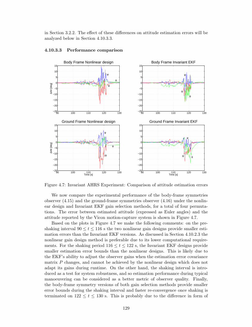
in Section 3.2.2. The effect of these differences on attitude estimation errors will beanalyzed below in Section 4.10.3.3.
4.10.3.3 Performance comparison
90 100 110 120 130−25
−20
−15
−10
−5
0
5
10
15
∆Att
[deg
]
φ
θ
ψ
Body Frame Nonlinear design
90 100 110 120 130−25
−20
−15
−10
−5
0
5
10
15
φ
θ
ψ
Body Frame Invariant EKF
90 100 110 120 130−25
−20
−15
−10
−5
0
5
10
15
∆Att
[deg
]
φ
θ
ψ
Ground Frame Nonlinear design
Time [s]90 100 110 120 130
−25
−20
−15
−10
−5
0
5
10
15
φ
θψ
Ground Frame Invariant EKF
Time [s]
Figure 4.7: Invariant AHRS Experiment: Comparison of attitude estimation errors
We now compare the experimental performance of the body-frame symmetriesobserver (4.15) and the ground-frame symmetries observer (4.16) under the nonlin-ear design and Invariant EKF gain selection methods, for a total of four permuta-tions. The error between estimated attitude (expressed as Euler angles) and theattitude reported by the Vicon motion-capture system is shown in Figure 4.7.
Based on the plots in Figure 4.7 we make the following comments: on the pre-shaking interval 90 ≤ t ≤ 116 s the two nonlinear gain designs provide smaller esti-mation errors than the Invariant EKF versions. As discussed in Section 4.10.2.3 thenonlinear gain design method is preferable due to its lower computational require-ments. For the shaking period 116 ≤ t ≤ 122 s, the Invariant EKF designs providesmaller estimation error bounds than the nonlinear designs. This is likely due tothe EKF’s ability to adjust the observer gains when the estimation error covariancematrix P changes, and cannot be achieved by the nonlinear design which does notadapt its gains during runtime. On the other hand, the shaking interval is intro-duced as a test for system robustness, and so estimation performance during typicalmanoeuvering can be considered as a better metric of observer quality. Finally,the body-frame symmetry versions of both gain selection methods provide smallererror bounds during the shaking interval and faster re-convergence once shaking isterminated on 122 ≤ t ≤ 130 s. This is probably due to the difference in form of
129

invariant output errors Ea and Em in the two designs discussed in Section 4.10.3.2:for the body-frame version, errors in attitude R and measurements ya, ym multiplywhich provides an attenuating effect assuming the errors are smaller than unity. Bycontrast the ground-frame invariant output errors Ea, Em superimpose attitude andmeasurement errors, which does not provide this attenuation effect. In this sensethe body-frame version is superior for experiment even though the ground-frameversion has the theoretical advantage of guaranteeing global existence of the movingframe γ(x), c.f. Section 4.10.2.2.
4.11 Invariant Aided INS testing
4.11.1 Implementation details
We now implement the Aided INS invariant observers designed in Section 4.7.2 andsummarized below. As mentioned at the end of Section 4.8 a nonlinear observergain design for this case is not available, hence we use the Invariant EKF methodof gain assignment (c.f. Section 4.9) whose (A,B,C,D) matrices were designed inSection 4.9.3 and will be summarized below.
As discussed in Section 4.5 the Aided INS outputs (4.7) assume the rotationmatrix RNE and navigation frame location roE are found during an initializationperiod, such that the vehicle’s CM position measurement yp = pN in navigationframe coordinates is converted from the GPS measurement raE of the tail-mountedantenna position in ECEF frame coordinates by
yp = pN = REN (raE − roE)−RlB
where lB is the antenna lever-arm vector, c.f. Section 3.2.3.2. The GPS receiverreports the discrete-time covariance σ2p,d and solution status of every measurement.
The former is converted to continuous-time covariance σ2p = E〈νpνTp 〉 in the naviga-tion frame by (c.f. Section 3.2.7)
σ2p = TGPS
(RENσ
2p,dR
NE
)
where TGPS = 0.01 s is the nominal period between GPS measurements. The so-lution status is used to determine whether or not the current yp is used for aiding;we employ the same criterion as in Section 3.2.10.2 i.e. only measurements withfloating narrow-lane ambiguity or better are used for aiding. The second Aided INSoutput is the magnetometer measurement ym = RTm where m is the local magneticfield vector in the navigation frame, available from a reference model as discussedin Section 2.8. Magnetometer measurements are corrected using the full compen-sation method in Section 2.9, such that as in Section 3.2.2, ym = Acm + bc and(σcm)
2 = Acσ2m(Ac)
T are the compensated aiding measurement and its covariancematrix, where m is provided by the on-board triaxial magnetometer and σ2m is theidentified covariance of its measurements. The measurement noise covariance ma-trix Rν = diag(σ2p, (σ
cm)
2) is used together with the process noise covariance matrixQν = diag(σ2f , σ
2ω, σ
2bf , σ
2bω) and the linearized system’s (A,B,C,D) matrices in the
130

Invariant EKF computation (4.26) to obtain the matrix of observer gains
K =
Lpp LpmLvp LvmLRp LRmLbfp LbfmLbωp Lbωm
The identified values of sensor covariances σ2 are available from Table 3.1 in Sec-tion 3.2.2. The Invariant Aided INS observers are numerically implemented usingthe modified Euler method discussed in Section 4.10.1. Similarly to Section 4.10.3,if a position aiding measurement yp is rejected due to insufficient precision of theGPS solution, the observer correction is skipped for this instant of time, increasingthe time step h used by the observer at the next aiding measurement.
4.11.1.1 Body frame symmetries
From Section 4.7.2.1, the Aided INS body-frame symmetries observer is (4.17)
˙p = v + LppEp + LpmEm
˙v = R(f − bf )− a+ LvpEp + LvmEm
˙R = RS(ω − bω) + S
[LRp Ep + LRmEm
]R
˙bf = RT
(Lbfp Ep + LbfmEm
)
˙bω = RT
(Lbωp Ep + LbωmEm
)
with invariant output errors
[EpEm
]=
[p− yp
m− Rym
]
The gains L are then computed using the Invariant EKF method with the set ofmatrices from Section 4.9.3.1
A =
0 I 0 0 0
0 0 −S[R(f − bf )] −I 00 0 0 0 −I0 0 0 S[R(ω − bω)] 0
0 0 0 0 S[R(ω − bω)]
B =
0 0 0 0
−R 0 0 0
0 −R 0 0
0 0 R 0
0 0 0 R
C =
[−I 0 0 0 00 0 −S(m) 0 0
]D =
[−I 0
0 −R
]
131

4.11.1.2 Ground frame symmetries
From Section 4.7.2.2, the Aided INS ground-frame symmetries observer is (4.18)
˙p = v + R(LppEp + LpmEm
)
˙v = R(f − bf )− a+ R(LvpEp + LvmEm
)
˙R = RS(ω − bω) + RS
[LRp Ep + LRmEm
]
˙bf = Lbfp Ep + LbfmEm
˙bω = Lbωp Ep + LbωmEm
with invariant output errors
[EpEm
]=
[RT (p− yp)
RTm− ym
].
The gains L are computed using the Invariant EKF method employing the matricesin Section 4.9.3.2
A =
−S(ω − bω) I 0 0 0
0 −S(ω − bω) −S(f − bf ) −I 0
0 0 −S(ω − bω) 0 −I0 0 0 0 00 0 0 0 0
B =
0 0 0 0−I 0 0 00 −I 0 00 0 I 00 0 0 I
C =
[−I 0 0 0 0
0 0 −S(RTm) 0 0
]D =
[−RT 00 −I
]
4.11.2 Simulation results
4.11.2.1 Hover Simulation
The first simulation test is a hover manoeuver identical to that in Section 3.4.1.1: thevehicle starts off on the ground with φ0 = θ0 = 0 i.e. level and ψ0 = π/2 i.e. facinggeographic East and remains stationary for 45 s to simulate an initialization period.It then flies vertically up by 5 m in 5 s followed by a counter-clockwise turn of180 over 5 s to end up facing West. These position and attitude configurationsare connected using quintic and cubic splines, respectively. The resulting referencetrajectory is converted to magnetometer m, accelerometer f , rate gyro ω and GPSraE signals which are corrupted with simulated bias and noise using parameters fromTable 3.1 in Section 3.2.2 and employing a Gauss-Markov process model for thetime-varying bias terms. The noisy sensor log is used as an input to the body-frameinvariant Aided INS observer (4.17) and ground-frame observer (4.18) using theInvariant EKF method of gain selection with Q and R covariance matrix entriestaken from Table 3.1 and initial error covariance P0 = 015×15, c.f. Section 4.10.1.The resulting state estimates are plotted in Figures 4.8 and 4.9 for the body-framesymmetry and ground-frame symmetry observers, respectively.
Both versions of the observer are shown to work and provide correct estimates ofthe position, velocity and attitude states of the hover manoeuver, which are essen-tially identical between the two designs. The estimated biases bf and bω vary slightly
132

45 50 55 60−10
0
10
p N [m
] p1
p2p
3
45 50 55 60−2
0
2v N
[m/s
]
v1
v2
v3
45 50 55 60−100
0
100
Att
[deg
]
φθ
ψ
Time [s]
45 50 55 600.09
0.1
0.11
0.12
0.13
b f [m/s
2 ]
bf,1
bf,3
bf,2
45 50 55 600.018
0.019
0.02
0.021
0.022
b ω [r
ad/s
]
Time[s]
bω,2
bω,1bω,3
Figure 4.8: Body-Frame Invariant Aided INS: Simulated Hover
45 50 55 60−10
0
10
p N [m
] p1
p2p
3
45 50 55 60−2
0
2
v N [m
/s]
v1
v2
v3
45 50 55 60−100
0
100
Att
[deg
]
φθ
ψ
Time [s]
45 50 55 600.09
0.1
0.11
0.12
0.13
b f [m/s
2 ]
bf,1
bf,3
bf,2
45 50 55 600.018
0.019
0.02
0.021
0.022b ω
[rad
/s]
Time[s]
bω,2
bω,1 bω,3
Figure 4.9: Ground-Frame Invariant Aided INS: Simulated Hover
between the two observer versions, likely caused by differences in the symbolic formsof the two observers and associated IEKF matrices affecting the numerical integra-tion, for instance the estimated attitude R enters the bf and bω dynamics in thebody-frame symmetries observer (4.17) but not in the ground-frame symmetriesobserver (4.18). These differences are small, however, and the main point of thissimulation is to establish that both versions of the invariant observer work correctly.
4.11.2.2 Trajectory Simulation
The next simulation involves the figure-8 trajectory from Section 3.4.1.2 with posi-tion and attitude described by the parametric curves (3.27) and (3.28) using the sameparameter values as before: major and minor diameters of M = 50 m, m = 25 mfor each lobe, a vertical delta of H = 10 m and the geometric center of the figure-8placed at pN = (0, 0,−15) m with a full circuit flight period of T = 50 s. Thesimulated vehicle starts out level and stationary on the ground with ψ0 = 90 for45 s, then the trajectory splines into the full-speed figure-8 flight over 10 s. Thesame Invariant EKF parameters as in Section 4.11.2.1 are used here. The stateestimates for the body-frame and ground-frame symmetries observers are shown inFigures 4.10 and 4.11, respectively.
As in Section 4.11.2.1, both versions of the invariant observer are confirmed towork for the simulated trajectory. The flight states are estimated correctly and only
133

50 100 150 200 250−50−25
02550
p N [m
] p1 p
2
p3
50 100 150 200 250−8−4
048
v N [m
/s] v
1 v2
v3
50 100 150 200 250−270−180−90
090
Att
[deg
] φθ
ψ
Time [s]
50 100 150 200 2500.06
0.08
0.1
0.12
0.14
0.16
b f [m/s
2 ] bf,1
bf,3
bf,2
50 100 150 200 2500.016
0.018
0.02
0.022
0.024
b ω [r
ad/s
]
Time[s]
bω,2
bω,1 bω,3
Figure 4.10: Body-Frame Invariant Aided INS: Simulated Figure-8 flight
50 100 150 200 250−50−25
02550
p N [m
] p1p
2
p3
50 100 150 200 250−8−4
048
v N [m
/s] v
1 v2
v3
50 100 150 200 250−270−180−90
090
Att
[deg
] φθ
ψ
Time [s]
50 100 150 200 2500.06
0.08
0.1
0.12
0.14
0.16
b f [m/s
2 ] bf,1
bf,3
bf,2
50 100 150 200 2500.016
0.018
0.02
0.022
0.024b ω
[rad
/s]
Time[s]
bω,2
bω,1
bω,3
Figure 4.11: Ground-Frame Invariant Aided INS: Simulated Figure-8 flight
small discrepancies are visible between the two designs. This is more clearly seen inFigure 4.12, where we plot the error between the estimated states and the generatedreference trajectory for each observer.
−0.060
0.06
∆pN
−0.10
0.1
∆vN
−202
∆Att
−0.050
0.05
∆bf
50 100 150 200 250−4
04x 10
−3
∆bω
Time [s]
−0.060
0.06
∆pN
−0.10
0.1
∆vN
−202
∆Att
−0.050
0.05
∆bf
50 100 150 200 250−4
04x 10
−3
∆bω
Time [s]
Figure 4.12: Invariant Aided INS: Simulated Figure-8 flight estimation errors: Body-frame symmetry; Ground-frame symmetry
134

4.11.3 Experimental results
4.11.3.1 Ground Test
This test uses sensor logs from the experiment described in Section 3.4.2: the engine-off helicopter is manually carried around the periphery of a rectangular landingpad at the flight field, held level with its heading aligned with the direction oftravel and executing a 90 counter-clockwise turn at every corner for two completecircuits. The experiment includes an initialization period where the helicopter isleft stationary and level at the southern-most corner of the pad aligned with theinitial direction of travel; the helicopter is also set down at this spot once its circuitis complete. We employ the magnetometer compensation technique described inSection 2.9 using parameters from Table 2.1 to construct the termsAc and bc. We usethe same observer parameters as for the simulations in Sections 4.11.2.1 and 4.11.2.2,namely Invariant EKF process and measurement covariance matrices Q and R fromTable 3.1 and initial estimation error covariance matrix P0 = 015×15. The resultingstate estimates are plotted in Figure 4.13 for the body-frame symmetries invariantobserver and Figure 4.14 for the ground-frame version.
40 60 80 100 120 140 160−10
0
10
20
p N [m
] p1
p2
p3
40 60 80 100 120 140 160−2−1
012
v N [m
/s] v
1
v2
v3
40 60 80 100 120 140 160−180−90
090
180
Att
[deg
]
φθ
ψ
Time [s]
40 60 80 100 120 140 160−0.2
0
0.2
0.4b f [m
/s2 ]
bf,1
bf,2b
f,3
40 60 80 100 120 140 160
−0.02
0
0.02
0.04
b ω [r
ad/s
]
Time [s]
bω,1bω,2
bω,3
Figure 4.13: Body-Frame Invariant Aided INS: Experimental engine-off walk
40 60 80 100 120 140 160−10
0
10
20
p N [m
] p1
p2
p3
40 60 80 100 120 140 160−2−1
012
v N [m
/s] v
1
v2
v3
40 60 80 100 120 140 160−180−90
090
180
Att
[deg
]
φθ
ψ
Time [s]
40 60 80 100 120 140 160−0.2
0
0.2
0.4
b f [m/s
2 ]
bf,1
bf,2
bf,3
40 60 80 100 120 140 160
−0.02
0
0.02
0.04
b ω [r
ad/s
]
Time [s]
bω,1bω,2
bω,3
Figure 4.14: Ground-Frame Invariant Aided INS: Experimental engine-off walk
Similarly to the simulation case, the two invariant observer versions performvery similarly to each other. Remark the non-zero component of vN during thepre-pickup t ≤ 60 s due to the use of 3-axis magnetometer updates as discussed in
135

Section 3.4.2.1; unlike Figure 3.12, however, the error is eliminated by the invariantobserver adjusting estimates of bf,1 and bf,2, such that the end velocity is correctlyestimated as zero. The position and attitude estimates are qualitatively correct:p1 and p2 show the circuit trajectory is repeated exactly twice, p3 identifies thepick-up and set-down times of the helicopter, φ and θ and kept near zero due to thehelicopter being level while ψ increases by 90 at each (counter-clockwise) cornerturn. Although an exact reference is not available (unlike the AHRS experiment inSection 4.10.3), we can use the measured dimensions of the landing pad and its yawangle w.r.t. geographic North to create an approximated reference trajectory for theoverhead position and yaw angle. This is done in Figure 4.15 for the body-frameand ground-frame symmetries observers. The two versions are seen to provide goodperformance relative to the available reference.
−5 0 5
0
2
4
6
8
10
12
p2 (E) [m]
p 1 (N
) [m
]
Body Frame Invariant EKF
−5 0 5
0
2
4
6
8
10
12
p2 (E) [m]
p 1 (N
) [m
]
Ground Frame Invariant EKF
40 60 80 100 120 140 160−180
−135
−90
−45
0
45
90
135
180
Time [s]
ψ [d
eg]
Body Frame Invariant EKF
40 60 80 100 120 140 160−180
−135
−90
−45
0
45
90
135
180
Time [s]
ψ [d
eg]
Ground Frame Invariant EKF
Figure 4.15: Invariant Aided INS: Experimental engine-off walk comparison: Body-frame symmetry; Ground-frame symmetry
4.11.3.2 Flight Test
The final experimental test is the engine-on hover flight previously seen in Sec-tion 3.4.3. The helicopter starts out stationary on the landing pad running theengine in idle setting. The throttle input is then increased, causing the main rotorto spool up until lift-off is achieved. After a transient take-off phase a stable hoveris achieved characterized by a near-constant yaw angle provided by the tail gyro’sheading-hold mode; the helicopter still drifts around due to strong cross-winds andconstant stick input from the pilot required to maintain stable hover. The helicopterthen lands.
136

Table 4.1: Engine-on Invariant Aided INS observer parametersBody Frame Invariant EKF
diag(Qf ) diag(Qω) diag(Qbf ) diag(Qbω) diag(Rm)[m2/s3] [rad2/s] [m2/s4] [rad2/s2] [G2 s]
100 · 0.00792 10 · 0.00172 1 · 0.00422 1 · 0.000292 50 · 0.000582100 · 0.00742 10 · 0.00172 1 · 0.00202 1 · 0.000382 50 · 0.000512100 · 0.00902 10 · 0.00212 1 · 0.00162 1 · 0.000322 50 · 0.000512
Ground Frame Invariant EKF
diag(Qf ) diag(Qω) diag(Qbf ) diag(Qbω) diag(Rm)[m2/s3] [rad2/s] [m2/s4] [rad2/s2] [G2 s]
100 · 0.00792 10 · 0.00172 0.01 · 0.00422 0.01 · 0.000292 50 · 0.000582100 · 0.00742 10 · 0.00172 0.01 · 0.00202 0.01 · 0.000382 50 · 0.000512100 · 0.00902 1 · 0.00212 0.01 · 0.00162 0.01 · 0.000322 50 · 0.000512
The key challenge is the uncertainty in noise and bias modeling for the engine-on case. As noted in Section 3.4.3, the identified noise characteristics from theengine-off case as well as initial error covariance matrix P0 entries must be tuned tomake the filter work in the engine-on case. In addition the noise characteristics varywith time, e.g. the spool-up resonant frequency effect discussed in Section 3.4.3.1. Asexplained below we found it necessary to adjust the Invariant EKF Q and R matricesdifferently for the body-frame and ground-frame symmetries cases as summarizedin Table 4.1. In addition, we set the initial bias estimation error covariances ofbf , bω in P0 as follows: for the body-frame case, Pf,1 = Pf,2 = 1 × 10⁻³; Pf,3 =1 × 10⁻⁷; Pω,1 = Pω,2 = 1 × 10⁻⁵; Pω,3 = 1 × 10⁻⁷; for the ground-frame case,Pf,1 = Pf,2 = Pf,3 = 1 × 10⁻⁴ and Pω,1 = Pω,2 = Pω,3 = 1 × 10⁻⁵. The resultingestimates are plotted in Figure 4.16 for the body-frame version and Figure 4.17 forthe ground-frame version.
40 60 80 100 120 140 160 180−4−2
0246
p N [m
] p1
p2
p3
40 60 80 100 120 140 160 180−2−1
012
v N [m
/s] v
1
v2
v3
40 60 80 100 120 140 160 180−20
0204060
Att
[deg
]
φθ
ψ
Time [s]
40 60 80 100 120 140 160 180−0.8−0.6−0.4−0.2
00.20.40.6
b f [m/s
2 ] bf,1
bf,2 b
f,3
40 60 80 100 120 140 160 180−0.02
00.020.040.060.08
b ω [r
ad/s
]
Time [s]
bω,1
bω,2 bω,3
Figure 4.16: Body-Frame Invariant Aided INS: Experimental engine-on hover
Unlike the results in Section 4.11.2 and Section 4.11.3.1, there is a noticeabledifference in performance between the body-frame and ground-frame version of theobserver, with the latter performing much closer to the conventional EKF versionplotted in Figure 3.15 in Section 3.4.3.1; the nearly constant ψ provided by theheading-hold tail gyro is clearly visible in Figure 4.17 but not in Figure 4.16. Theground-frame version is also the case reported in [18].
137

40 60 80 100 120 140 160 180−4−2
0246
p N [m
] p1
p2
p3
40 60 80 100 120 140 160 180−2−1
012
v N [m
/s] v
1
v2
v3
40 60 80 100 120 140 160 180−20
0204060
Att
[deg
]
φ
θ
ψ
Time [s]
40 60 80 100 120 140 160 180−0.8−0.6−0.4−0.2
00.20.40.6
b f [m/s
2 ] bf,1
bf,2
bf,3
40 60 80 100 120 140 160 180−0.02
00.020.040.060.08
b ω [r
ad/s
]
Time [s]
bω,1
bω,2
bω,3
Figure 4.17: Ground-Frame Invariant Aided INS: Experimental engine-on hover
The reason for the discrepancy and need for different observer parameters can beexplained by looking at the form of the body-frame invariant observer (4.17) summa-rized in Section 4.11.1.1 versus the ground-frame observer (4.18) in Section 4.11.1.2:the estimated attitude R enters the bias bf , bω dynamics in the former but not inthe latter. This means that any errors in estimated attitude immediately affect thebias estimates in the body-frame version, which further aggravates the problem dueto bω used for the high-rate integration of R dynamics. Remark that in the ground-frame observer (4.18) the estimated attitude R enters the p and v dynamics whereasit does not in the body-frame observer (4.17). Indeed zooming in on the estimatedposition pN for the pre-takeoff period of 55 ≤ t ≤ 70 s as shown in Figure 4.18,we see the body-frame version provides better position estimates (p closer to zero)than the ground-frame version. However, given that position is directly aided bythe GPS modulo the lever-arm term, the ground-frame invariant observer is morerobust to poor bias and sensor noise modeling than the body-frame version as seenin Figures 4.16 and 4.17. Of course a better model of the engine-on noise charac-teristics would reduce this discrepancy, as seen in the engine-off experimental testsin Section 4.11.3.1 where the noise parameters are well-identified [75, Chap. 4].
60 65 70
−0.2
−0.1
0
0.1
0.2
p N [m
]
Time [s]
Body Frame Invariant EKF
p1
p2
p3
60 65 70
−0.2
−0.1
0
0.1
0.2
p N [m
]
Time [s]
Ground Frame Invariant EKF
p1
p2
p3
Figure 4.18: Invariant Aided INS: Pre-takeoff estimated position zoom-in view
138

Chapter 5
Nonlinear Model of a Helicopter
UAV
5.1 Overview
The dynamics of the helicopter are governed by the 6 DoF nonlinear equationsof motion of a rigid body [105, p. 167] whose forcing terms are gravity as well asforce and moment vectors created by aerodynamic effects, both controlled (e.g. rotorthrust) and uncontrolled (e.g. drag forces), which must be modeled as functions ofthe vehicle state and pilot inputs.
In contrast to rigid-body dynamics, aerodynamics are much more complicatedto model due to the large number of physical processes involved, including unsteadyflow through the rotating helicopter blades, wake-body interactions, vortex forma-tion and turbulence at the rotor tips, blade stall, flow compressibility effects andaeroelasticity of the blades. High-fidelity helicopter models use a finite-element ap-proach to accurately model the physics of the flow. For control design, the betterapproach is to use lumped-parameter models of the individual helicopter subsystems— main rotor, main rotor blade flapping, fuselage body, tail horizontal stabilizer,tail vertical stabilizer and tail rotor — using simplified aerodynamics equations,whose parameters are experimentally identified and can be further adjusted to tunethe model output to match experimental flight data. This “minimum-complexity”approach [65], originally applied to full-sized helicopter modeling and control studiescarried out by NASA [43] has been used for helicopter UAVs in [101, 59, 21] withexcellent results.
A visual representation of the proposed model structure is shown in Figure 5.1.The rigid-body equations of motion are derived in Section 5.2. We develop expres-sions for the individual subsystems’ forces and moments as functions of the helicopterstate and pilot inputs throughout Section 5.3. The resulting model is summarizedin Section 5.4 and its identified parameter values are listed in Section 5.5.
5.2 Rigid-Body Model
In this Section, we derive the 6 DoF rigid-body dynamics governing the motion of thehelicopter, shown schematically in Figure 5.2. The ground-fixed (inertial) navigationframe has orthonormal basis vectors (n1, n2, n3) and the body-fixed (non-inertial)
139

xb
yb
zb
Tmr
Qmr
a1
b1
mg
Ffus
Ttr
Fhs
Fvs
Figure 5.1: Helicopter Model: Overall View [59]
body frame has orthonormal basis vectors (b1, b2, b3). The origin of the B frame isplaced at the centre of mass of the helicopter.
n1n2
n3
b1b2
b3
p
pp
pCM
rp
Figure 5.2: Navigation and Body Frames on Helicopter
By inspection of Figure 5.2, the position of any point p on the helicopter body isdescribed by the vector pp = pCM + rp where by construction pp and pCM start atthe N frame origin while rp starts at the B frame origin. Using frame coordinatesthis is written as
ppN (t) = pCMN (t) +R(t)rpB ,
where the rotation matrix R(t) ∈ SO(3) is the coordinate transformation matrixfrom B to N . Physically, R measures the attitude of the helicopter, e.g. R = Imeans the B and N frames are aligned and so the helicopter is level with zero yaw.Differentiating with respect to time gives
vpN (t) = vCMN (t) + R(t)rpB , (5.1)
where vpN (t) and vCMN (t) := vN (t) are the velocities of p and the centre of massw.r.t. the navigation frame origin.
The linear momentum vector of a point mass m is G = mv and its angularmomentum vector about a point P is HP = dP ×mv where dP denotes the vector
140

from P to the mass. The linear momentum vector of a rigid body is defined as theintegral of infinitesimal linear momentums, i.e.
G =
∫
Vvp dm, (5.2)
where vp is the velocity vector of the infinitesimal mass element dm = ρ dV , wherevp and mass density ρ vary over the volume. Similarly, the angular momentumvector of the rigid body about a point P is defined by
HP =
∫
VdP × vp dm, (5.3)
with dP the position vector from P to dm. The G and HP vectors are expressed inthe same frame as their integrands, i.e. using (5.1) in (5.2) gives
GN (t) =
∫
V
(vN (t) + R(t)rpB
)dm = vN (t)
∫
Vdm+ R(t)
∫
VrpB dm = mvN (t) (5.4)
where m is the total mass of the body. The second integral in (5.4) is zero byconstruction: the CM position vector p of a rigid body is defined by
p :=1
m
∫
Vpp dm,
but due to placing the B frame origin at the centre of mass, we have pp = rp,p = r = 0 and rB = 0 =⇒
∫V r
pB dm = 0. Next, using (5.1) in (5.3) and taking
P = CM we have
HCMN (t) =
∫
VdCMN (t)× vN (t) dm+
∫
VdCMN (t)× R(t)rpB dm (5.5)
Using dCMN (t) = R(t)dCMB and dCMB = rpB the first integral in (5.5) becomes∫
VR(t)rpB × vN (t) dm = −vN (t)×R(t)
∫
VrpB dm = 0
due to∫V r
pB dm = 0 as above. Using the rotational kinematics R(t) = R(t)S
(ωB(t)
)
where ω(t) is the angular velocity vector and S is the skew-symmetric matrix suchthat x × y = S(x)y, x, y ∈ R
3 along with the identity S(Rx) = RS(x)RT , R ∈SO(3), the second integral in (5.5) becomes
∫
VR(t)rpB ×R(t)S
(ωB(t)
)rpB dm = R(t)
∫
VS(rpB)S
(ωB(t)
)rpBdm.
Denoting rpB = [x y z]T and ωB(t) = [p q r]T the integrand becomes
S(rpB)S(ωB(t))rpB =
0 −z yz 0 −x−y x 0
0 −r qr 0 −p−q p 0
xyz
=
−rxz + pz2 − qxy + py2
−ryz + qz2 + qx2 − pxyry2 − qyz + rx2 − pxz
=
y2 + z2 −xy −xz−xy x2 + z2 −yz−xz −yz x2 + y2
︸ ︷︷ ︸I
pqr
︸︷︷︸ωB(t)
.
141

Returning to (5.5) we have
HCMN (t) = R(t)
∫
VIωB(t)dm = R(t)JωB(t) (5.6)
where J =∫V I dm is the inertia matrix, a function of the geometry and mass
distribution of the body. Remark I hence J is symmetric and so it is always diag-onalizable. Physically this corresponds to correctly orienting the body-fixed frameB, whose origin is still required to be taken at the centre of mass. In this caseJ = diag(Jxx, Jyy , Jzz) and (b1, b2, b3) define the principal axes of the body. Fornow we leave J as a general (non-diagonalized) inertia matrix.
The dynamics of a rigid body are governed by Euler’s laws of motion
F =d
dtG(t) and MCM =
d
dtHCM (t), (5.7)
where F , MCM are the net external force and moment vectors acting on the body.Equations (5.7) hold under the following conditions:
• The mass of the body must remain constant,
• The moment and angular momentum vectors must be taken about the centreof mass of the body,
• The linear and angular momentum vectors must be expressed in an inertialframe.
Note it is possible to treat systems which do not meet one or more of these con-ditions by generalizing the laws of motion. The case of time-varying mass, impor-tant in e.g. rocketry where the fuel burn rate creates a significant loss in mass istreated in [99, Art. 53]. Taking the angular momentum about a general, possiblyaccelerating point will be developed in Section 5.2.2 and involves defining an an-gular momentum relative to the moving point. Finally, it is possible to formulatethe problem in a non-inertial frame by using the principles of relative motion [99,Art. 38], which transforms the velocity and acceleration observed in a non-inertialframe to their absolute values by employing the acceleration and rotation of thenon-inertial frame. The present system avoids these complications, however, andso (5.7) holds.
Using the linear momentum vector (5.4) (expressed in inertial frame N) in (5.7)gives
FN (t) =d
dt
(mvN (t)
)=⇒ FN (t) = m ˙vN (t), (5.8)
i.e. the familiar F = ma. It is possible to express (5.8) in the body frame, for reasonswhich will be explained shortly. We have
R(t)FB(t) =d
dt
(mR(t)vB(t)
)
= mR(t)vB(t) +mR(t) ˙vB(t)
= mR(t)S(ωB(t))vB(t) +mR(t) ˙vB(t)
R(t)FB(t) = mR(t)ωB(t)× vB(t) +mR(t) ˙vB(t),
142

and left-multiplying by RT (t) yields
FB(t) = m(ωB(t)× vB(t) + ˙vB(t)
), (5.9)
the body-frame version of F = ma where v = [u v w]T denotes the velocityvector of the helicopter’s CM expressed in body frame components. Although (5.9)is more complicated than (5.8), the reason for using it is that the aerodynamic forces,e.g. the main rotor thrust, are naturally formulated in the body-fixed B frame. Theone exception is gravity which always acts downwards and must be transformed intoB frame coordinates as RT (t)gN where gN = [0 0 g]T .
Using (5.6) (taken about CM and expressed in the inertial frame N as required)in (5.7) gives
MCMN (t) =
d
dt
(R(t)JωB(t)
)
= R(t)JωB(t) +R(t)JωB(t)
MCMN (t) = R(t)S(ωB(t))JωB(t) +R(t)JωB(t)
R(t)MCMB (t) = R(t)ωB(t)× JωB(t) +R(t)JωB(t).
Left-multiplying by RT (t) then gives
MCMB (t) = ωB(t)× JωB(t) + JωB(t). (5.10)
Together (5.9) and (5.10) are known as the Newton-Euler equations, e.g. [105,p. 167], which govern the translational and rotational dynamics of the helicopter.
As discussed above, the J matrix can be diagonalized by properly orientingthe B frame axes. We assume the helicopter’s roll-pitch-yaw axes are sufficientlyaligned with the principal axes such that J ≈ diag(Jxx, Jyy, Jzz). Although thisassumption is not required, it greatly simplifies the form of (5.10) and has beenused in other experimentally-validated helicopter models [59, 101, 122]. Expandingout (5.9) and (5.10) with gravity force mgB = mRTgN we obtain
u = rv − qw +R31g +X/m
v = pw − ru+R32g + Y/m
w = qu− pv +R33g + Z/m
p = qr(Jyy − Jzz)/Jxx + L/Jxx
q = pr(Jzz − Jxx)/Jyy +M/Jyy
r = pq(Jxx − Jyy)/Jzz +N/Jzz
(5.11)
where (X,Y,Z), (L,M,N) are the components of the aerodynamic force and mo-ment vectors expressed in the roll-pitch-yaw body frame, respectively. The dynam-ics (5.11) are integrated to obtain vB = [u v w]T , ωB = [p q r]T which in turnare integrated through the kinematics
R = RS(ωB)
pN = RvB(5.12)
to obtain attitude and position of the helicopter with respect to the ground-fixednavigation frame.
143

The mass m in (5.11) is measured directly using a digital scale. The location ofthe CM was identified by balancing the side of the helicopter on a knife-edge andis shown in Figure 5.3, where the CM is located on the vertical centerline plane ofthe vehicle. The mass moment of inertias Jxx, Jyy and Jzz were first attempted tobe measured using a trifilar pendulum apparatus [114, p. 3.18] as suggested by [36,Sec. 6.3.2.2], however this method proved unusable due to lateral swinging motionsof the helicopter during experimental testing [53]. We then successfully obtainedthe values using a torsional pendulum apparatus described in Section 5.2.1.
Figure 5.3: Helicopter UAV with identified CM location
5.2.1 Torsional Pendulum
The torsional pendulum system is sketched in Figure 5.4. A circular disk with massm0, radius r0 and mass moment of inertia J0 (around the vertical axis) rotates byangle θ as shown. The disk is supported by three long, thin wires of uniform lengthl, fixed above the disk and attached at the outer rim.
ll
l
m0, r0, J0
θ
Figure 5.4: Torsional pendulum schematic
We derive the pendulum’s equation of motion using Lagrange’s equation. Sincethe top supports are fixed and the cables have constant lengths, the disk must moveupwards when it rotates away from its neutral configuration. Consider the sideview of a single cable subject to a disk rotation of θ, shown in Figure 5.5. The cablebottom advances by r0θ units horizontally, while the whole disk rises vertically byh.
From Figure 5.5, we immediately see h = l −√l2 − r20θ
2. The Lagrangian
144

ll
r0θh
Figure 5.5: Geometry of support cable; disk rotated by θ
L = T − V , the difference between kinetic and potential energy, is
L =1
2J0(θ)
2 −m0g
(l −√l2 − r20θ
2
),
from which the equation of motion is obtained by
d
dt
(dL
dθ
)− dL
dθ= 0 =⇒ J0θ +
m0gr20θ√
l2 − r20θ2= 0,
a nonlinear ODE. Consider the denominator of the second term,
l
l
√l2 − r20θ
2 = l
√1−
(r0l
)2θ2.
If the support cables are made much longer than the disk radius, r0/l << 1 andhence (r0/l)
2 ≈ 0. The equation of motion then becomes
J0θ +m0gr
20
lθ = 0,
an undamped linear oscillator with natural frequency
ω2n =
m0gr20
J0l. (5.13)
Equation (5.13) is used to find J0 by giving the disk an initial rotation then allowingit to oscillate back-and-forth about its vertical centerline. The period of oscillationT = 2π/ωn is directly measured and substituted into the above to solve for J0.
Consider a body with (known) mass m and (unknown) mass moment of inertiaJ . The body is rigidly attached to the disk in Figure 5.4, such that the verticaldisk axis passes through the center of mass of the measured object. The derivationabove now uses mass m0 +m and inertia J0 + J , giving the natural frequency
ω2n =
(m0 +m)gr20(J0 + J)l
=
(2π
T
)2
,
where T is the period of oscillation of the composite system. Solving for the unknowninertia,
J =(m0 +m)gr20T
2
4π2l− J0 (5.14)
145

the measured body’s mass moment of inertia about the vertical axis, so the mea-surement is performed for the yaw, pitch and roll axes of the helicopter, the lastrequiring using a stand attached to the disk in order to hold the helicopter in po-sition. The stand must be accounted for by measuring its mass ms and identifyingJ0 of the disk-stand assembly using Equation (5.13) with mass term (m0+ms). Wealso reiterate the need for the support cables to be as long as possible such that thelinearizing approximation holds. Pictures of the experimental setup for the pitchand roll axes are shown in Figure 5.6; remark the stand used for the roll axis as wellas the hanging weight used to align the helicopter’s CM with the center of the diskbelow it. The computed Jxx, Jyy , Jzz values are provided in Section 5.5.
Figure 5.6: Experimental measurement of J using a torsional pendulum [53]: pitchaxis, roll axis.
5.2.2 Extended Moment Equation
As mentioned in Section 5.2, it is possible to generalize the second Euler equa-tion (5.7) to take moments about a general (non-CM) point. This will be used inSection 5.3.1.3 to derive the flapping dynamics of the main rotor.
A general rigid body is shown schematically in Figure 5.7 where N is the ground-fixed inertial frame, B is the body-fixed frame with point o on its origin, p is anarbitrary point on the body, pp and po are the position vectors from the origin of Nto points p and o, respectively, while rp is the position vector from the origin of Bto p. The rigid body and its attached frame B are free to accelerate. By definitionthe rigid body possesses a center of mass, but its coordinates are not important atthe moment.
By inspection of Figure 5.7 we have the vector expression ppN (t) = poN (t) +rpN (t) whose components are functions of time due to the motion of the rigid body.
146

N
oB
ppo
pp
rp
Figure 5.7: Rigid body with body frame fixed at arbitrary point o
Differentiating with respect to time we obtain
vpN (t) = voN (t) + vpN (t) (5.15)
where vpN (t) := (d/dt)rpN (t) physically represents the relative velocity of point p withrespect to point o; remark vpN is a non-inertial measurement if o is accelerating.Following (5.3) we define the relative angular momentum of the body as
HoN (t) =
∫
VrpN (t)× vpN (t)dm (5.16)
Since HoN (t) is not taken about the centre of mass or a fixed point, Euler’s equa-
tions (5.7) do not apply directly. Instead we take the time derivative of (5.16) andobtain
d
dtHoN (t) =
∫
VvpN (t)× vpN (t)dm+
∫
VrpN (t)× apN (t)dm,
where apN (t) := (d/dt)vpN (t) is the relative acceleration of point p w.r.t. point o, anon-inertial measurement if the body is accelerating. The first integrand above iszero. Differentiating (5.15) we obtain apN (t) = apN (t)− aoN (t), a difference of inertialaccelerations. We have
d
dtHoN (t) =
∫
VrpN (t)× apN (t)dm−
∫
VrpN (t)× aoN (t)dm.
The first integrand contains apN (t)dm = dF pN , the external force acting on the in-finitesimal point p with mass dm. We thus have
∫V r
pN (t) × dF pN = Mo
N , the netexternal moment about point o acting on the rigid body. The second integral be-comes
−∫
VrpN (t)× aoN (t)dm = aoN (t)×
∫
VrpN (t)dm = aoN (t)×mrCMN (t)
by definition of center of mass location rCM = 1m
∫V rdm; physically rCMN (t) repre-
sents the position vector from o to the CM expressed in N frame coordinates. Wehave obtained
d
dtHoN (t) =Mo
N −mrCMN (t)× aoN (t). (5.17)
147

We now return to (5.16). Using rpN (t) = R(t)rpB and vpN (t) = (d/dt)rpN (t) =R(t)rpB = R(t)S
(ωB(t)
)rpB we have
HoN (t) =
∫
VR(t)rpB ×R(t)S
(ωB(t)
)rpBdm
Just as in Section 5.2 we use the identity S(Rx) = RS(x)RT , R ∈ SO(3) and obtain
HoN (t) = R(t)
∫
VS(rpB)S
(ωB(t)
)rpBdm := R(t)
∫
VIoωB(t)dm = R(t)JoωB(t)
where we wrote rpB = [xo yo zo]T and defined
Io =
(yo)2 + (zo)2 −xoyo −xozo
−xoyo (xo)2 + (zo)2 −yozo−xozo −yozo (xo)2 + (yo)2
and Jo =
∫
VIodm.
Remark Io resp. Jo are taken about o whereas I and J in Section 5.2 were takenabout the CM; the mass moments of inertia can be related using the parallel-axistheorem Jo = J +m‖rCM‖2. Taking the time derivative of the last Ho
N (t) abovegives
d
dtHoN (t) = R(t)JoωB(t) +R(t)JoωB(t) = R(t)S
(ωB(t)
)JoωB(t) +R(t)JoωB(t),
and substituting this into (5.17) gives
R(t)S(ωB(t)
)JoωB(t) +R(t)JoωB(t) =Mo
N −mrCMN (t)× aoN (t)
which is pre-multiplied by RT (t) to give
MoB = ωB(t)× JoωB(t) + JoωB(t) +mrCMB × aoB(t), (5.18)
the “extended” [33, p. 363] version of the Euler equation (5.10) from Section 5.2. Asexpected setting rCMB = 0 in (5.18) recovers (5.10) since in this case the moment istaken about the CM. Alternatively, setting aoB(t) = 0 gives Mo
B = ωB(t)×JoωB(t)+JoωB(t), the dynamics of a rigid body rotating about a fixed (or more generally non-accelerating) point o [99, Art. 25].
5.3 Aerodynamics and Subsystem Modeling
5.3.1 Main Rotor
The following suite of assumptions is used for modeling the main rotor [61, 42]:
• Rotor blades are rigid in bending and torsion
• Both the flapping angle β and inflow angle Φ are assumed small
• The effects of helicopter body motion on flapping are limited to the helicopter’sangular velocities p, q, angular accelerations p, q and normal acceleration (aB ·b3)
148

• The reversed flow region is ignored and compressibility and stall effects disre-garded
• The inflow is assumed uniform across the rotor disc and no inflow dynamicsare used
• Tip loss is neglected
The above assumptions are considered valid for advance ratios µ = V/(ΩR) < 0.3where V is the helicopter’s forward velocity. For the Bergen Industrial Twin withΩ = 1650 RPM and R = 0.810 m, this works out to V < 42 m/s, well above themaximum speeds achievable in forward flight.
5.3.1.1 Induced Velocity
The main rotor consists of two airfoil blades rotating clockwise at a rate of Ω. Asthe blades rotate, a mass flow of air is sucked through the rotor disc traced outby the spinning blades (illustrated in Figure 5.1) which generates a reaction forceperpendicular to the rotor disc known as the thrust T . The average velocity of theairstream passing through the rotor disc is known as the induced velocity vi, whichis understood to be parallel to the thrust vector.
We first consider the hover case, where the relationship between vi and resultingthrust T is worked out using control volume analysis [104, Ch. 5], assuming the flowis steady, inviscid and incompressible and using the stream tube shown in Figure 5.8as the control volume.
T
vi
v2
A1
A
A2
Figure 5.8: Rotor inflow in hover
In Figure 5.8, the fully developed wake region has stream tube area A2 andaverage flow velocity v2. The top of the stream tube A1 represents an area farupstream of the flow where the velocity is zero; A is the area of the rotor disc andis known from the helicopter blade length. The continuity equation gives ρAvi =ρA2v2 = m, the mass flow rate. The momentum equation gives Fcv =
∫cs vρv · ndA,
and since v0 = 0 the force on the flow Fcv = 0−v2ρv2A2 =⇒ T = v22ρA2, the reactionforce on the helicopter body. Finally the energy equation gives Wcv =
∫cs ερv · ndA
where W is the rate of work done on the flow and ε is the total specific energy ofthe flow, taken as the kinetic energy ε = v2/2 since we neglect changes in internaland potential energy. We know Wcv = Tvi, the power imparted to the flow by thehelicopter rotor, so Tvi = (v22/2)ρv2A2 =⇒ vi = v2/2 using the momentum equation.
149

Using the continuity equation we also have A/2 = A2, the wake contraction shownin Figure 5.8. Using the last two results we obtain T = 2v2i ρA.
The same control volume analysis applies in vertical flight where the helicopter inFigure 5.8 is climbing with velocity V . In this case, the flow velocity at A1 is V , thevelocity through the rotor disc A is V +vi, and the wake velocity at A2 is V +v2. Thecontinuity equation gives m = ρA1V = ρA(V + vi) = ρA2(V + v2), the momentumequation gives Fcv = V ρV A1−(V +v2)ρ(V +v2)A2 = V m−(V +v2)m =⇒ T = v2mand the energy equation gives Wcv = −1
2V2ρV A1 + 1
2 (V + v2)2ρ(V + v2)A2 =⇒
T (V + vi) = V v2m + 12v
22m. Combining the last two results gives v2m(V + vi) =
V v2m+ v22/2m =⇒ vi = v2/2, just as in the hover case, and so T = 2vi(V + vi)ρAwhich correctly reduces to the hover thrust expression above when V = 0.
Di
T
V∞ vi
αi
αi
Figure 5.9: Rotor inflow in fast forward flight
Fast forward flight is shown schematically in Figure 5.9. As before, we assumeuniform inflow vi across the rotor disc; based on experimental testing results [115,p. 124] this assumption is not as accurate as in the hover case, however this ismitigated by the fact that V ≫ vi [72, p. 126]. In order to obtain a relationshipbetween vi and T , we view the rotor disc as a fixed, finite-width wing and employlifting-line theory [13, Sec. 5.3], where vi is the downwash which reduces the effectiveangle of attack of the wing and creates the induced drag Di parallel to the localinflow. This is illustrated in Figure 5.9, where the rotor must generate the induceddrag force Di in addition to the usual thrust force T to maintain unacceleratedflight. We assume an elliptical distribution of circulation across the wing, which isknown to yield uniform downwash over the span of the wing [13, p. 411] as desired.For the elliptical distribution, the relationship between lift and drag is analyticallycalculated to be [13, Eq. (5.43)]
CD,i =C2L
πAR,
where CD,i = Di/(q∞S) is the coefficient of induced drag with q∞ = (1/2)ρ∞V∞the free-stream dynamic pressure and S the wing planform area; CL = L/(q∞S) isthe coefficient of lift with L = T perpendicular to the local inflow; and AR = b2/Sis the wing aspect ratio with b the span of the wing. For the helicopter rotor discb = 2R and S = πR2 = A where R is measured from the blade geometry (A waspreviously used in Figure 5.8). From Figure 5.9 we have
tanαi =viV∞
=CD,iCL
=C2L
πARCL=
T12ρ∞V
2∞Sπ(2R)
2/S=⇒ vi =
T
2ρ∞V∞A
150

We now seek a universal expression for vi which applies to any flight conditionof the helicopter. The control volume used for this analysis is shown in Figure 5.10.The stream velocity V shown corresponds to the helicopter flying up and forwards.The velocities perpendicular to the horizontal cross-sections with areas A1, A andA2 are thus V sinα, V sinα+vi and V sinα+v2, respectively, where vi is the inducedvelocity at the rotor and v2 is the downstream induced velocity as in the verticalclimb case.
A1
A
A2
V Tα
vi
Figure 5.10: Rotor inflow in general flight
The continuity equation∫cs ρv · ndA = 0 gives ρV sinαA1 = ρ(V sinα+ vi)A =
ρ(V sinα + v2)A2 ≡ m, the mass flow rate perpendicular to the horizontal cross-sections. The momentum equation Fcv =
∫cs vρv · ndA along the vertical direc-
tion gives F vcv = V sinαρV sinαA1 − (V sinα + v2)ρ(V sinα + v2)A2 =⇒ T =−V sinαm+(V sinα+v2)m = v2m. Finally, the energy equation Wcv =
∫cs ερv ·ndA
where ε represents the specific kinetic energy of the flow (1/2)v2 gives T (V sinα+vi) = −(1/2)V 2ρV sinαA1 + (1/2)[(V cosα)2 + (V sinα+ v2)
2]ρ(V sinα+ v2)A2 =−(1/2)V 2m+(1/2)[V 2+2V v2 sinα+v
22 ]m⇒ V v2 sinαm+(1/2)v22m = v2m(V sinα+
vi) ⇒ v2 = 2vi just as in the hover and vertical climb cases. The momentum equa-tion thus becomes T = 2vim. Although m represents the vertical mass flow rate,following [62] we redefine m = ρAU where U =
√(V cosα)2 + (V sinα+ vi)2 is
the total velocity of the stream at the rotor disc. Using this definition the inducedvelocity is
vi =T
2ρA√
(V cosα)2 + (V sinα+ vi)2. (5.19)
For vertical climb α = π/2 and (5.19) becomes vi = T/(2ρA(V + vi)) which agreeswith the earlier analysis. For fast forward flight α = 0, V ≫ vi and (5.19) becomes
vi = T/(2ρA√V 2 + v2i ) ≈ T/(2ρAV ) which also agrees with the previous analysis.
This is precisely the reason for redefining m as above; although this step is notmathematically rigorous, [72, Sec. 4-1.1] points out that vi predicted by (5.19) agreeswith experimental data as well as more complicated theories. The result has beenaccepted in newer helicopter books [115, 113] and used in experimentally-validatedhelicopter models [59, 21]. Remark (5.19) is an implicit equation for vi which canbe solved using numerical root-finding [72, p. 129].
151

5.3.1.2 Blade lift and drag
A cross-section of the main rotor blade airfoil with infinitesimal width dl and chordlength c is shown in Figure 5.11 where Θ is the blade pitch angle, (UT , UP ) are thetangential and perpendicular components of the approaching airstream vector withinflow angle Φ, α is the angle of attack of the airfoil and dL, dD are the resultinglift and drag forces, respectively, which by definition are perpendicular and parallelto the incoming airstream vector.
UP
UT
Θ
Φα
dL
dD
c
Figure 5.11: Blade cross-section
In the absence of stall, the lift force dL acting on the airfoil section is
dL =1
2ρU2CLcdl,
where ρ is air density as before, U = (U2T+U
2P )
1/2 is the airstream vector magnitude,c is the chord length of the airfoil and CL is the coefficient of lift. The drag forceon the airfoil is
dD =1
2ρU2CDcdl,
where CD is the coefficient of drag. The values of CL and CD versus angle of attackα can be obtained from wind tunnel experiments and are tabulated based on airfoilgeometry, discussed below, and Reynolds number
Re :=ρV c
µ(5.20)
where µ = 1.789 × 10⁻⁵ N s/m2 is the dynamic viscosity of air at ground altitudeby the International Standard Atmosphere (ISA).
The main rotor blade is a symmetric airfoil with chord length c = 66.3 mm andmaximum thickness t = 9.3 mm at x = 19 mm from the leading edge; these valueswere directly measured using a digital caliper. Based on the ratios t/c = 0.14,x/c = 0.29 the blade is classified as a NACA 0014 airfoil [8, p. 114], where thefirst two integers indicate percent camber and fractional location from the leadingedge (00 for a symmetric airfoil), and the last two integers indicate the maximumthickness in percent of the chord, which by definition occurs at x/c = 0.3 in all4-digit NACA series airfoils. Experimental data plots for CL vs α as well as CDvs α for a variety of airfoils and Reynolds numbers — see e.g. [8, pp. 462-463] fora NACA 0012 airfoil at Re = 3 × 10⁶, 6 × 10⁶, 9 × 10⁶ — show that CL is a linear
152

function of α and CD is nearly constant with α for roughly |α| ≤ 10. For symmetricairfoils we denote
CL = aα
where a is the slope of the lift curve in its linear range.Experimental data is not always available for all airfoil shapes, e.g. [8] does
not include NACA 0014 data. In this case the alternative approach is a numericalcalculation of the lift and drag forces, which can be done analytically for “thin”airfoils (t/c ≤ 0.12) by modeling them as a vortex sheet [13, Sec. 4.7], or for moregeneral airfoil shapes by using the vortex panel numerical method [13, Sec. 4.10].The latter method is implemented by the online applet JavaFoil1 which lets the userspecify the airfoil geometry according to NACA series and computes the lift anddrag coefficients as a function of Reynolds number and range of angles of attack.The Reynolds number for the main blades is obtained from (5.20) using V = ΩRwith Ω = 55π rad/s and R = 0.810 m giving Re ≈ 6× 10⁵. The resulting plots areshown in Figure 5.12 and the lift curve slope a and drag coefficient CD are obtainedusing a least-squares fit in the linear range; remark α is reported in degrees and theslope value is converted to CL/rad to obtain a.
0 2 4 6 8 10 12 14 160
0.2
0.4
0.6
0.8
1
1.2
1.4
α [deg]
CL
0 2 4 6 8 10 12 14 160
0.02
0.04
0.06
0.08
0.1
0.12
α [deg]
CD
Figure 5.12: NACA 0014 data from JavaFoil: Coefficients of lift and drag vs angleof attack
We now obtain expressions for the aerodynamic force components dF⊥ and dF ‖
perpendicular and parallel to the tangential airstream UT which will be used inSections 5.3.1.3 and 5.3.1.5 below. From Figure 5.11 we have α = Θ−Φ where theinflow angle Φ is assumed small (c.f. Section 5.3.1) and so Φ = arctan(UP /UT ) ≈UP /UT . Due to the high rotational speed of the main rotor U2
T ≫ U2P and so
U2 = U2T + U2
P ≈ U2T . Since CL is typically an order of magnitude larger than CD
as seen in Figure 5.12 we can neglect the contribution of dD to dF⊥, although wecannot make this assumption for dF ‖. The resulting expressions are
dF⊥ = dL cos Φ− dD sinΦ ≈ dL =1
2ρac
(ΘU2
T − UTUP)dl
dF ‖ = dL sinΦ + dD cos Φ ≈ ΦdL+ dD =1
2ρac
(ΘUTUP − U2
P
)dl +
1
2ρcCDU
2Tdl
(5.21)
1http://www.mh-aerotools.de/airfoils/javafoil.htm
153

5.3.1.3 Main rotor flapping dynamics
Each rotor blade is an airfoil rotating at the rate Ω whose azimuth ψ denotes theclockwise angle from the tail boom. The blade is allowed to move up and downrelative to the helicopter’s horizontal plane either via a hinge mounted near therotor hub, as done in full-sized helicopters, or by a combination of blade bendingand an elastomeric flapping restraint, the latter design known as a “hingeless” rotorwhich is typically used on RC helicopters including our Bergen Industrial Twin.The helicopter head design, to be discussed in Section 5.3.2, generates the periodicblade pitch
Θ = A0 +A1 cosψ +B1 sinψ (5.22)
where A0, A1 and B1 are directly controlled through a series of mechanical link-ages. Since the lift force on an airfoil is proportional to its pitch angle, the A1,B1 coefficients in (5.22) cause periodic up/down motion of each blade known asflapping, causing the rotor disc and thrust vector to tilt about the longitudinal andlateral axes, respectively, providing underactuated control over 4 of the 6 DoF’s ofthe helicopter.
The flapping dynamics are obtained by performing a moment balance on anindividual blade, modeled as a rigid body hinged at the main rotor shaft and shownschematically in Figure 5.13. The blade is modeled as a uniform thin plate withlinear mass density ρb and length R. The blade’s flapping angle β is measured fromthe helicopter’s horizontal plane. The torsional spring kβ is a lumped model ofthe elastomeric flapping restraint and the blade’s elasticity, producing the restoringmoment −kββ about the flapping axis. The flapping motion is also forced by theinfinitesimal aerodynamic force dF⊥ which must be integrated along the length,and the blade weight mR acting at the CM located at l = R/2 since the blade wasassumed uniform. The blade’s angular velocity is a combination of β plus main rotorspeed Ω and the body’s roll and pitch rates p and q, respectively. In addition, thehinge point undergoes linear acceleration az along the helicopter’s normal direction(b3 axis) as assumed in Section 5.3.1, i.e. we neglect the ax and ay components. Theactual expression for this term is obtained from (5.11) resp. (5.9) as az = w+pv−qu,specifically the third component of the inertial acceleration vector of the helicopter’sCM expressed along the body-fixed frame.
kβ
Ω
−kβββ
p
q
az
(mR)g
dF⊥
l = R
Figure 5.13: Main Rotor: Blade free-body diagram
The moment balance on the blade in Figure 5.13 will be performed about theflapping hinge such that reaction forces can be neglected. We place the blade-fixedframe at the flapping hinge as shown in Figure 5.14 where the frame’s i, j and k
154

axes are aligned with the blade’s feathering, flapping and lagging axes, respectively.We will employ the generalized moment equation (5.18) developed in Section 5.2.2.
β
ψ
Ω
p
qij
k
Figure 5.14: Blade flapping kinematics
The blade-fixed frame in Figure 5.14 is aligned with the symmetry axes of theblade and so Jo = diag(Joxx, J
oyy , J
ozz). The blade is modeled as a thin plate of width
w, thickness t, length R and total mass M = mR. The components of Jo areobtained from standard mass moment of inertia expressions, e.g. [100, p. 713], thenapproximated using t≪ w. We get
Joxx =1
12M(w2 + t2) ≈ 1
12Mw2
Joyy =1
12Mt2 +
1
3MR2 ≈ 1
3MR2
Jozz =1
12Mw2 +
1
3MR2 = Joxx + Joyy
(5.23)
We write MoB = [Lo Mo No]T , ωB = [pb qb rb]T and aoB = [aox aoy aoz]
T
which represent the body-frame vector components of the total external momentabout the hinge axis, inertial angular velocity of the blade and inertial linear ac-celeration of the hinge point, respectively. We have rCMB = [R/2 0 0]T since theblade is uniform. Using these in (5.18) along with Jo = diag(Joxx, J
oyy , J
ozz) and total
blade mass mR, we obtainLo
Mo
No
=
qbrb(Jozz − Joyy)
pbrb(Joxx − Jozz)pbqb(Joyy − Joxx)
+
Joxxp
b
Joyy qb
Jozz rb
+mR
0−(R/2)aoz(R/2)aoy
Flapping takes place around the j axis so we employ only the second component ofthe above equations. Using Joxx − Jozz = −Joyy from (5.23) and defining Jβ := Joyy,Mβ := ρbR
2/2 as in [42] we obtain
Mo = Jβ qb − Jβp
brb −Mβaoz (5.24)
In Figure 5.13 we had az = w + pv − qu, the hinge’s inertial acceleration2 parallelto the helicopter’s b3 axis. For the blade-fixed frame shown in Figure 5.14 we have
aoz = (w + pv − qu) cos β (5.25)
2Recall we neglect the helicopter’s lateral accelerations ax and ay for analyzing the flappingdynamics, i.e. employ only the normal component az, by assumption from Section 5.3.1.
155
We also need expressions for pb, rb and qb = (d/dt)qb, the inertial angular accelera-tions of the blade expressed along the blade-fixed frame axes. These can be obtainedby inspection of Figure 5.14:
pb = −p cosψ cos β − q sinψ cos β − Ω sin β
qb = p sinψ − q cosψ + β
rb = −p cosψ sin β − q sinψ sin β +Ωcos β
Computing (d/dt)qb using ψ = Ω we get
qb = p sinψ + pΩcosψ − q cosψ + qΩ sinψ + β
The above are used to expand Jβ(qb−pbrb) in (5.24) and higher-order terms are sim-
plified as [42] cos2 β ≈ 1, sin2 β ≈ 0, p2 ≈ 0, q2 ≈ 0 and pq ≈ 0; the simplificationsare justified by small flapping angles β and p, q ≪ Ω. The result is
Jβ(qb−pbrb) = Jβ
(β+p sinψ−q cosψ+2pΩcosψ+2qΩ sinψ+Ω2 cos β sinβ
)(5.26)
The net moment about the flapping hinge Mo consists of the three external forcesshown in Figure 5.13: the blade weight moment Mw = −(mR)g(R/2) cos β =−Mβg cos β; the torsional spring restoring moment Mkβ = −kββ; and the aero-
dynamic moment MA =∫ R0 ldF⊥ where dF⊥ is given by (5.21) in Section 5.3.1.2.
Based on Figure 5.14 the blade cross-section at azimuth ψ and distance l from theflapping axis experiences the airstream velocity components
UT = Ωl cos β + u sinψ − v cosψ
UP = (vi −w) cos β + u sin β cosψ + v sin β sinψ + βl + pl sinψ − ql cosψ(5.27)
where [u v w]T is the body-frame component velocity of the helicopter, vi is theinduced velocity covered in Section 5.14, and p, q are the helicopter roll and pitchrates as before. The aerodynamic moment integral is
MA =
∫ R
l=0ldF⊥ =
1
2ρac
∫ R
l=0l(ΘU2
T − UTUP
)dl
Substituting Θ from (5.22) and UP , UT from (5.27) into the integrand and assumingsmall flapping angles such that cosβ ≈ 1, sin β ≈ β gives
MA =1
24ρacR2
− 2R
[pu+ qv + 2Ω(vi − w)
]
+[6viv − 6vw +RΩ(3Rq − 4uβ)
]cosψ
+ 2[R(pu− qv) + 3uvβ
]cos 2ψ −
[6viu− 6uw +RΩ(3Rp+ 4vβ)
]sinψ
+[2R(qu+ pv) + 3β(−u2 + v2)
]sin 2ψ + (A0 +A1 cosψ +B1 sinψ)
[3(u2 + v2 + (RΩ)2)− 8RΩv cosψ − 3(u2 − v2) cos 2ψ
+ 8RΩu sinψ − 6uv sin 2ψ]−Rβ
[3RΩ− 4v cosψ + 4u sinψ
]
(5.28)
156

Returning to (5.24), using (5.25), (5.26) assuming a small β angle and employingMo =Mw +Mkβ +MA gives the governing equation for the flapping angle β of anindividual blade:
β+p sinψ−q cosψ+2pΩcosψ+2qΩ sinψ+Ω2β =Mβ
Jβ(w+pv−qu−g)−kβ
Jββ+
1
JβMA
Substituting (5.28) into the above gives a linear, second-order, non-homogenousdifferential equation for β(t):
β +ρacR3
24Jβ
3RΩ− 4v cosψ + 4u sinψ
β +
(kβJβ
+Ω2
)
+ρacR2
24Jβ
(4RΩu cosψ − 6uv cos 2ψ + 4RΩv sinψ + 3(u2 − v2) sin 2ψ
)β
=Mβ
Jβ
(w + pv − qu− g
)− p sinψ + q cosψ − 2pΩcosψ − 2qΩ sinψ
+ρacR2
24Jβ
− 2R
[pu+ qv + 2Ω(vi − w)
]+ 3[2viv − 2vw +R2Ωq
]cosψ
+ 2R(pu− qv) cos 2ψ − 3[2viu− 2uw +R2Ωp
]sinψ + 2R(qu+ pv) sin 2ψ
+ (A0 +A1 cosψ +B1 sinψ)[3(u2 + v2 + (RΩ)2)− 8RΩv cosψ
− 3(u2 − v2) cos 2ψ + 8RΩu sinψ − 6uv sin 2ψ]
(5.29)In order to get an expression for the flapping dynamics in the helicopter-fixed (non-rotating) frame, we use the classical method [61, p. 153] of writing the 2π-periodicβ(t) as a Fourier series then neglecting all second and higher harmonics:
β(t, ψ) ≈ a0(t)− a1(t) cosψ + b1(t) sinψ (5.30)
where a0, a1 and b1 physically represent the coning, longitudinal tilt and lateraltilt angles of the rotor disc traced out by the tips of the spinning blades, andthe a1, b1 signs have been assigned for consistency with Figure 5.1 on p. 140. Thisapproach is justified by experiment, where the amplitude of in-plane weaving (secondharmonic) is an order of magnitude smaller than the coning and tilting motion.Differentiating (5.30) twice with respect to time, we obtain
β = a0 − a1 cosψ + a1Ω sinψ + b1 sinψ + b1Ωcosψ
= a0 + (−a1 + b1Ω) cosψ + (a1Ω+ b1) sinψ (5.31)
β = a0 − a1 cosψ + 2a1Ω sinψ + a1Ω2 cosψ + b1 sinψ + 2b1Ωcosψ − b1Ω
2 sinψ
= a0 + (−a1 + a1Ω2 + 2b1Ω) cosψ + (2a1Ω+ b1 − b1Ω
2) sinψ (5.32)
Expressions (5.32), (5.31) and (5.30) are then substituted into the LHS of (5.29)and the coefficients of the constant, cosψ and sinψ terms are matched in order toobtain the dynamics of x = [a0 a1 b1]
T , the tip path plane angles resulting in thesystem x+Dx+K = F .
157

Based on the results in [42], we are able to pre-simplify our expressions. A keyparameter in flapping dynamics is the Lock number
γ :=ρacR4
Jβ
For the Bergen Industrial Twin, using the identified parameters given in Section 5.5we compute γ = 4.03 and by [42, Fig. 8], we see that the advance ratio µ hasnegligible effect on the flapping modes for this “low” (γ < 8) Lock number. Thismeans we can disregard the translational velocity terms u, v in (5.29), whose LHSbecomes
β +ρacR3
24Jβ
3RΩ
β +
kβJβ
+Ω2
β = β +
γΩ
8β +
(kβJβ
+Ω2
)β
Substituting (5.32), (5.31) and (5.30) into the above and grouping terms yields
a0 +γΩ
8a0 +
(kβJβ
+Ω2
)a0 +
− a1 + a1Ω
2 + 2b1Ω+γΩ
8(−a1 + b1Ω)
−(kβJβ
+Ω2
)a1
cosψ+
2a1Ω+b1−b1Ω2+
γΩ
8(a1Ω+b1)+
(kβJβ
+Ω2
)b1
sinψ
while the RHS of (5.29) with u = v = 0 is
Mβ
Jβ
(w − g
)− p sinψ + q cosψ − 2pΩcosψ − 2qΩ sinψ +
γ
24R2
− 4RΩ(vi − w)
+ 3R2Ωq cosψ − 3R2Ωp sinψ + (A0 +A1 cosψ +B1 sinψ)[3(RΩ)2
]
Matching the constant, cosψ and sinψ coefficients gives
a0 +γΩ
8a0 +
(kβJβ
+Ω2
)a0 =
Mβ
Jβ
(w − g
)− γΩ
6R(vi − w) +
γΩ2
8A0
−a1 + 2b1Ω+γΩ
8(−a1 + b1Ω)−
kβJβa1 = q − 2pΩ+
γΩ
8q +
γΩ2
8A1
2a1Ω+ b1 +γΩ
8(a1Ω+ b1) +
kβJβb1 = −p− 2qΩ− γΩ
8p+
γΩ2
8B1
(5.33)The first equation describes the dynamics of the coning mode a0, with naturalfrequency ω0 =
√kβ/Jβ +Ω2 and forcing terms consisting of normal motion w and
w, gravity g and collective pitch A0; it can be verified ζ0 = (γΩ)/(16ω0) althoughthis term is not required in the sequel. The remaining two equations are a coupleddynamics system for flapping angles a1, b1, which can be rewritten in the formx+Dx+Kx = F as
[a1b1
]+
[γΩ8 −2Ω
2Ω γΩ8
] [a1b1
]+
[ kβJβ
−γΩ2
8γΩ2
8kβJβ
][a1b1
]=
[−q + 2pΩ− γΩ
8 q −γΩ2
8 A1
−p− 2qΩ− γΩ8 p+
γΩ2
8 B1
]
(5.34)
158

The natural frequencies and damping ratios of (5.34) can be calculated using themethod of complex modal analysis [70, pp. 332–334]. The homogenous versionof (5.34) x+Dx+Kx = 0 is written in state-space form by defining x1 = x, x2 = x:
[x1x2
]=
[0 I
−K −D
] [x1x2
]
The eigenvalues of the above matrix are two complex-conjugate pairs λ1 and λ2,corresponding to the system’s two vibration modes, whose natural frequencies anddamping ratios are respectively calculated by
ωi =√
Reλi2 + Imλi2 and ζi =−Reλi√
Reλi2 + Imλi2
By direct computation we find
λ1 = −γΩ16
± j
4Jβ
√32(JβΩ)2 + 16Jβkβ −
1
16(γJβΩ)2 + 2JβΩ ξ
λ2 = −γΩ16
± j
4Jβ
√32(JβΩ)2 + 16Jβkβ −
1
16(γJβΩ)2 − 2JβΩ ξ
ξ :=√
256(JβΩ)2 + 256Jβkβ − (γJβΩ)2
Remark the only difference between the two eigenvalue pairs is the sign in front ofthe ξ term. We then have
ω1 =
(Ω2 + ω2
0 +Ω
8
√(16ω0)
2 − (γΩ)2)1/2
ζ1 =γΩ
16ω1
ω2 =
(Ω2 + ω2
0 −Ω
8
√(16ω0)
2 − (γΩ)2)1/2
ζ2 =γΩ
16ω2
where
ω0 =
(Ω2 +
kβJβ
)1/2
is the frequency of the coning mode as before. The vibration modes characterizedby (ω1, ζ1) and (ω2, ζ2) are known as the advancing and regressing flapping modes,respectively. As discussed in [42] we retain only the regressive flapping mode, whosefrequency is sufficiently low to couple into the rigid-body motions of the helicopter.A good approximation of this mode can be obtained by setting a1 = b1 = 0 in (5.34).Further, for this low-frequency effect we can omit the effect of angular accelerationsby setting p = q = 0. The flapping dynamics become simplified to
2b1Ω+γΩ
8(−a1 + b1Ω)−
kβJβa1 = −2pΩ+
γΩ
8q +
γΩ2
8A1
2a1Ω+γΩ
8(a1Ω+ b1) +
kβJβb1 = −2qΩ− γΩ
8p+
γΩ2
8B1
Remark each of the cyclic inputs A1 and B1 affects both a1 and b1 in the simplifiedequations above. In reality, the control linkages are designed to achieve perfect 90
159

phase lag between cyclic input and maximum flapping angle in order to decouple theflapping response. Mathematically, this means that in steady-state, the A1 cyclicpitch component should affect only the lateral flapping angle b1 and the B1 only thelongitudinal a1; this is done by dropping the a1 term from the first equation and theb1 term from the second one in the simplified model above, as seen in [101, p. 73]who uses this approach without comment. The regressing mode dynamics become
2b1Ω+γΩ
8(b1Ω)−
kβJβa1 = −2pΩ+
γΩ
8q +
γΩ2
8A1
2a1Ω+γΩ
8(a1Ω) +
kβJβb1 = −2qΩ− γΩ
8p+
γΩ2
8B1
and interchanging their order and normalizing the coefficients of A1, B1 gives
16
γΩa1 + a1 =
−8kβγΩ2Jβ
b1 −16
γΩq − 1
Ωp+B1
16
γΩb1 + b1 =
8kβγΩ2Jβ
a1 −16
γΩp+
1
Ωq +A1
(5.35)
The dynamics (5.35) are a highly simplified form of the flapping dynamics of themain rotor. They offer insight into the physics of flapping and can be used for asimulation model with some parameter identification, c.f. [65, p. 16]. A more com-plete model of the flapping dynamics can be obtained by returning to (5.29) andsubstituting the tip-path plane expression (5.30) but without neglecting transla-tional velocity terms as done in [42, 21], at the expense of a dramatic increase insymbolic complexity. The regressing mode approximation could also be avoided byusing (5.34) resp. (5.33) when integrating for the flapping dynamics. We will notpursue these avenues further.
5.3.1.4 Flapping Dynamics Simplifications
In Section 5.3.1.3 we have used identified parameters values for the Bergen IndustrialTwin to compute the Lock number γ = 4.03 and simplify the flapping dynamics.Using the same numerical approach we can obtain further simplifications of ourmodel.
The ANCL helicopter uses an approximate head speed of Ω = 1650 RPM =55π rad/s. We also use the following identified values from Section 5.5: kβ =122 Nm/rad; Jβ = 0.057 kgm2. We numerically compute the natural frequencyand damping ratio pairs for the coning (ω0, ζ0), advancing (ω1, ζ1) and regressing(ω2, ζ2) modes as
ω0 = 178.87 rad/s = 28.47 Hz ζ0 = 0.2433
ω1 = 349.01 rad/s = 55.55 Hz ζ1 = 0.1247
ω2 = 43.53 rad/s = 6.93 Hz ζ2 = 0.9999
As predicted only the regressing mode has a frequency low enough (6.93 Hz) topossibly couple into the motion of the helicopter body, although the other flappingfrequencies will show up in the frequency content of the IMU sensor signal. Re-mark the regressing mode is nearly critically damped and hence the approach ofapproximating it as a first-order system (5.35) is justified.
160

Using a 5% criterion the settling time for a unit step input into the regressingmode is given by [109, p. 233] ts = 3/(ζωn) = 0.069 s, or for the approximatesystem (5.35) with time constant τ = 16/(γΩ) this value is 3τ = 0.069 s, identicalto before. Based on these numbers we are justified in taking the flapping response ofthe main rotor as instantaneous. Physically this is due to the high angular speed ofthe main rotor (Ω = 1650 RPM = 27.5 Hz) which makes the transient period of theflapping dynamics negligibly short. This is the reason why a Bell-Hiller stabilizersystem, to be discussed in Section 5.3.2, is used on the Bergen Industrial Twin andother RC helicopters — to slow down the effective flapping response of the mainrotor and make the helicopter flyable for a human pilot. A new generation of flybar-less RC helicopters fly under closed-loop control and allow the pilot to tune themain rotor response in real-time to suit their preferences.
Neglecting the flapping dynamics of the main rotor is done by dropping the a1,b1 terms in (5.35). We can simplify further as follows: since the coning frequencyω0 =
√kβ/Jβ +Ω2 = 178.87 rad/s is less than 4% from the natural rotor frequency√
Ω2 = 172.79 rad/s, we can drop the kβ/Jβ term from (5.35). Evaluating the coef-ficients 16/(γΩ) = 0.023 and 1/Ω = 0.0058 we also see that the effect of on-axis andoff-axis angular rates on disc tilt is respectively two and three orders of magnitudelower than the cyclic amplitude terms A1 and B1. Under all these simplificationsequation (5.35) reduces to the steady-state expression
a1 = B1
b1 = A1(5.36)
In Section 5.3.1.5 we will develop the force and moment expressions for the mainrotor in full generality, i.e. leaving in the flapping dynamics, which can be neglectedlater by zeroing all a0, a1 and b1 terms.
5.3.1.5 Main Rotor Forces and Moments
We now calculate the force and moment vectors resulting from the aerodynamicforces acting on the main rotor. We first develop the fully general expressions thensimplify down to a hover model.
The main rotor thrust Tmr and counter-torque Qmr respectively defined as thenet body-vertical force and counter-clockwise moment in the body-horizontal planeare evaluated from
Tmr =Nb
2π
∫ 2π
0
∫ R
0dF⊥ cos β dψ
Qmr =Nb
2π
∫ 2π
0
∫ R
0l dF ‖ dψ
where Nb = 2 is the number of blades and dF⊥, dF ‖ are the perpendicular and par-allel aerodynamic forces acting on a blade section given by (5.21) in Section 5.3.1.2.We will also calculate Xmr, Ymr, the in-plane force parallel to the xb and yb axesgiven by
Xmr =Nb
2π
∫ 2π
0
(∫ R
0dF⊥ sin β cosψ −
∫ R
0dF ‖ sinψ
)dψ
Ymr =Nb
2π
∫ 2π
0
(∫ R
0dF⊥ sin β sinψ +
∫ R
0dF ‖ cosψ
)dψ
161

as well as Lmr, Mmr, the moments at the main rotor blade hub in aligned with thexb and yb axis directions:
Lmr =Nb
2π
∫ 2π
0
(∫ R
0l dF⊥ + kββ
)sinψ dψ
Mmr =−Nb
2π
∫ 2π
0
(∫ R
0l dF⊥ + kββ
)cosψ dψ
By assumption from Section 5.3.1 we take the flapping angle β as small such thatcos β ≈ 1 in T and sin β ≈ β in Xmr and Ymr above. The UT and UP expressionsin (5.27) simplify to
UT = Ωl + u sinψ − v cosψ
UP = vi − w + uβ cosψ + vβ sinψ + βl + pl sinψ − ql cosψ
The dF⊥, dF ‖ expressions in (5.21) as well as Θ, β and β in (5.22), (5.30) and (5.31)are repeated here for convenience:
dF⊥ =1
2ρac
(ΘU2
T − UTUP)dl
dF ‖ =1
2ρac
(ΘUTUP − U2
P
)dl +
1
2ρcCDU
2Tdl
Θ = A0 +A1 cosψ +B1 sinψ
β = a0 − a1 cosψ + b1 sinψ
β = a0 + (b1Ω− a1) cosψ + (a1Ω+ b1) sinψ
Using the expressions above we first evaluate the Tmr integral:
Tmr =ρacRNb
24
[4(RΩ)2 + 6(u2 + v2)
]A0 + 6RΩ
[w − vi − vA1 + uB1
]
− 3R[u(p + b1) + v(q + a1)
]− 4R2Ωa0
The p, b1 and q, a1 terms physically represent the lateral and longitudinal angularvelocity of the rotor disc, respectively. From Section 5.3.1.1 we know vi = vi(Tmr)and so Tmr is a transcendental equation which is typically solved numerically usingthe Newton-Rhapson method over a few iterations, e.g. [72, p. 129], [65, p. 18], [59,p. 35]. Since the transcendental equation is quartic it can be solved analyticallyas [21, p. 63], however this still does not provide an explicit Tmr expression due tothe requirement of selecting one of four possible solutions.
In hover with translational velocities, angular rates and flapping dynamics iden-tically zero, the Tmr expression reduces to
T hmr =ρacRNb
12
2(RΩ)2A0 − 3RΩvhi
(5.37)
where from Section 5.3.1.1
T hmr = 2(vhi )2ρπR2 =⇒ vhi =
√T hmr
2ρπR2(5.38)
162

We can obtain an explicit equation for T hmr by substituting (5.38) into (5.37), whichgives
T hmr =ρacR3NbΩ
2
6A0 −
acRNbΩ√ρ
4√2π
√T hmr := CTmrA0 −DT
mr
√T hmr
where by inspection CTmr, DTmr are positive constants. By defining x =
√T hmr we
can solve the above using the quadratic formula:
√T hmr =
−DTmr +
√(DT
mr)2 + 4CTmrA0
2or√T hmr =
−DTmr −
√(DT
mr)2 + 4CTmrA0
2
Squaring both sides gives
T hmr = CTmrA0 +(DT
mr)2
2±DT
mr
√CTmrA0 +
(DTmr)
2
4
In order to pick a single solution consider A0 = 0 for which
T hmr = (DTmr)
2 or T hmr = 0
but since zero collective pitch is known to produce zero thrust the “minus” solutionis the correct one:
T hmr = CTmrA0 +(DT
mr)2
2−DT
mr
√CTmrA0 +
(DTmr)
2
4(5.39)
Equation (5.39) is an explicit equation for hover thrust T hmr as a function of thecollective pitch angle A0 where CTmr, D
Tmr are constant parameters defined above.
A simplified expression for T hmr can be obtained by taking T hmr = mg in (5.38);this assumes zero acceleration along the zb axis
3. In this case (5.37) becomes
T hmr ≈ρacR3NbΩ
2
6A0 −
acRNbΩ
4
√mgρ
2π=⇒ T hmr ≈ CTmrA0 −DT
mr√mg
The assumption of zero zb axis acceleration is poor due to the constant adjustmentsof the collective input required to maintain hover; for this reason T hmr should becomputed using (5.39).
3This also assumes the helicopter is level, however this is reasonable since mg cosφ cos θ ≈ mg
for small angles.
163

The Qmr counter-torque expression evaluates to
Qmr =−ρacR2Nb
96
6(p2 + q2)R2 + 24(w − vi)
2 − 16R[qu− pv
]a0 + 12
[u2 + v2
]a20
+ 4[6u(w − vi) + 4vRΩ+ 3pR2Ω
]a1 + 3
[3u2 + v2 + 2(RΩ)2
]a21 − 12uva1b1
− 4[6v(w − vi) + 4uRΩ+ 3qR2Ω
]b1 + 3
[u2 + 3v2 + 2(RΩ)2
]b21
+ 4R[− 8w − 4ua1 + 4vb1 + 8vi + 3Ra0 − 3RΩA0 + 2vA1 − 2uB1
]a0
+ 2R[6qR− 8ua0 − 6RΩb1 + 3Ra1 − 4vA0 + 3RΩA1
]a1
+ 2R[6pR+ 8va0 + 6RΩa1 + 3Rb1 − 4uA0 − 3RΩB1
]b1
+ 8R[− pu− qv + 2wΩ − 2Ωvi
]A0
+[− 12v(w − vi) + 6qR2Ω− 8uRΩa0 − 3(u2 − v2)b1 − 6(RΩ)2b1 − 6uva1
]A1
+[12u(w − vi)− 6pR2Ω− 8vRΩa0 + 3(u2 − v2)a1 − 6(RΩ)2a1 − 6uvb1
]B1
+ρcR2CDNb
8
(RΩ)2 + u2 + v2
In hover with zero translational and rotational velocities and zero flapping dynamics,the above reduces to
Qhmr =−ρacR2Nb
96
24(−vhi )2 + 3
[2(RΩ)2
]a21 + 3
[2(RΩ)2
]b21 + 8R
[− 2Ωvhi
]A0
+[− 6(RΩ)2b1
]A1 +
[− 6(RΩ)2a1
]B1
+ρcR2CDNb
8
(RΩ)2
In hover (5.36) gives a1 = B1 and b1 = A1 and so Qhmr becomes
Qhmr =−ρacR2Nb
96
24(vhi )
2 + 6(RΩ)2a21 + 6(RΩ)2b21 − 16RΩvhi A0
− 6(RΩ)2b21 − 6(RΩ)2a21
+ρcR2CDNb
8
(RΩ)2
=ρacR2Nbv
hi
12RΩ
− 3RΩvhi + 2(RΩ)2A0
+ρcR4Ω2CDNb
8
=T hmrR
RΩ
√T hmr
2ρπR2+ρcR4Ω2CDNb
8:= CQmr
(T hmr
)3/2+DQ
mr (5.40)
where vhi was taken from (5.38), T hmr is calculated by (5.39) and CQmr, DQmr are
constants whose notation has been chosen to match [79, Sec. 2.2].
164

We now return to the Xmr and Ymr force expressions, which evaluate to
Xmr =−ρacRNb
96
24Rp(w − vi)
+ 4[18v(w − vi)− 2qR2Ω+ 3uRΩa0 + 12uva1 − 12v2b1 + 2(RΩ)2b1
]a0
+ 3R[pu− 5qv + 12Ω(w − vi) + 4Ωua1
]a1 − 12vRΩa1b1 + 3R
[qu− 7pv
]b1
− 4R[4pR+ 9va0 + 6RΩa1 − 3uA0 − 2RΩB1 + 4Rb1
]a0
−R[8RΩa0 + 15va1 − 3ub1 + 3uA1 − 3vB1
]a1
+R[24(w − vi) + 3ua1 − 21vb1 + 8RΩA0 − 3vA1 + 9uB1
]b1
+ 4[− 6u(w − vi) + 2pR2Ω+ 9vRΩa0 + 6v2a1 + 4(RΩ)2a1 + 6uvb1
]A0
−[3R(qu+ pv) + 24v2a0 + 8(RΩ)2a0 + 24vRΩa1
]A1
+ 3[3Rpu+Rqv − 4RΩ(w − vi) + 8uva0 + 4uRΩa1 + 4vRΩb1
]B1
− ρcR2ΩNb
4uCD
and
Ymr =−ρacRNb
96
24Rq(w − vi)
+ 4[− 18u(w − vi) + 2pR2Ω+ 3vRΩa0 − 12u2a1 + 2(RΩ)2a1 + 12uvb1
]a0
− 3R[pv − 7qu
]a1 − 12uRΩa1b1 + 3R
[5pu− qv − 12Ω(w − vi) + 4Ωvb1
]b1
− 4R[4qR − 9ua0 − 6RΩb1 − 3vA0 + 2RΩA1 + 4Ra1
]a0
+R[24(w − vi) + 21ua1 − 3vb1 + 8RΩA0 − 9vA1 + 3uB1
]a1
+R[8RΩa0 − 3va1 + 15ub1 − 3uA1 + 3vB1
]b1
− 4[6v(w − vi)− 2qR2Ω+ 9uRΩa0 + 6uva1 + 6u2b1 + 4(RΩ)2b1
]A0
+ 3[−Rpu− 3Rqv + 4RΩ(w − vi) + 8uva0 + 4uRΩa1 + 4vRΩb1
]A1
+[3R(qu+ pv)− 24u2a0 − 8(RΩ)2a0 − 24uRΩb1
]B1
− ρcR2ΩNb
4vCD
While the Xmr, Ymr terms are complicated, this is normal as evidenced by theexpressions found in e.g. [41, pp. 7-8]; [113, pp. 108-111]; [21, pp. 234-238]. In hoverwith u = v = w = 0, p = q = 0 and a0 = a1 = b1 = 0, the Xmr and Ymr expressions
165

simplify to
Xhmr =
−ρacRNb
96
[8(RΩ)2b1
]a0 −
[36RΩvhi
]a1
+[16(RΩ)2a1
]A0 −
[8(RΩ)2a0
]A1 +
[12RΩvhi
]B1
Y hmr =
−ρacRNb
96
[8(RΩ)2a1
]a0 +
[36RΩvhi
]b1
−[16(RΩ)2b1
]A0 −
[12RΩvhi
]A1 −
[8(RΩ)2a0
]B1
Using a1 = B1 and b1 = A1 from (5.36) we get
Xhmr =
−ρacRNb
96
−[24RΩvhi
]a1 +
[16(RΩ)2a1
]A0
=−ρacRNb
12
2(RΩ)2A0 − 3RΩvhi
a1
Y hmr =
−ρacRNb
96
[24RΩvhi
]b1 −
[16(RΩ)2b1
]A0
=ρacRNb
12
2(RΩ)2A0 − 3RΩvhi
b1
and using (5.37) we have
Xhmr = −T hmra1Y hmr = T hmrb1
which is validated by the flapping sign convention shown in Figure 5.1.The final set of calculations involve hub moment expressions Lmr, Mmr, which
turn out to have a simpler form than Qmr, Xmr and Ymr above:
Lmr =−ρacR2Nb
96
− 12uw + 12uvi + 6pR2Ω+ 8RvΩa0
+ 3[− u2 + v2 + 2(RΩ)2
]a1 + 6uvb1 + 8Rua0 + 6R2Ωb1
− 16uRΩA0 + 6uvA1 −[9u2 + 3v2 + 6(RΩ)2
]B1
+kβb1Nb
2
Mmr =−ρacR2Nb
96
− 12vw + 12vvi + 6qR2Ω− 8RuΩa0 − 6uva1
− 3[u2 − v2 + 2(RΩ)2
]b1 + 8Rva0 + 6R2Ωa1
− 16vRΩA0 +[3u2 + 9v2 + 6(RΩ)2
]A1 − 6uvB1
+kβa1Nb
2
At hover this reduces to
Lhmr =−ρacR2Nb
96
3[2(RΩ)2
]a1 −
[6(RΩ)2
]B1
+kβb1Nb
2=kβb1Nb
2= kβb1
Mhmr =
−ρacR2Nb
96
− 3[2(RΩ)2
]b1 +
[6(RΩ)2
]A1
+kβa1Nb
2=kβa1Nb
2= kβa1
where the second equality is due to a1 = B1 and b1 = A1 from (5.36) and the thirdfrom Nb = 2. The final result is validated by Figure 5.1 as well.
166

5.3.1.6 Main Rotor Contributions
The main rotor forces Tmr, Xmr and Ymr create a moment around the helicopter’sCM which is added to the moments Qmr, Lmr and Mmr. The main rotor’s forceand moment contributions along the helicopter’s body-fixed axes are given by
Xmr = Xmr
Ymr = Ymr
Zmr = −TmrLmr = hmrYmr + Lmr
Mmr = −hmrXmr +Mmr
Nmr = −Qmrwhere hmr is the height of the main rotor hub above the center of mass, measureddirectly using the identified CM position, c.f. Figure 5.3 in Section 5.2. The centerof mass is placed directly under the hub by moving the avionics box fore and aftin its T-slot rails attachment system. In hover the force and moment contributionsbecome
Xhmr = −T hmra1Y hmr = T hmrb1
Zhmr = −T hmrLhmr = hmrT
hmrb1 + kβb1
Mhmr = hmrT
hmra1 + kβa1
Nhmr = −CQmr
(T hmr
)3/2−DQ
mr
where by (5.39)
T hmr = CTmrA0 +(DT
mr)2
2−DT
mr
√CTmrA0 +
(DTmr)
2
4
and where we defined
CTmr :=ρacR3NbΩ
2
6DTmr :=
acRNbΩ√ρ
4√2π
CQmr :=1
RΩ√2ρπ
DQmr :=
ρcR4NbΩ2CD
8
The kβ term was used in Sections 5.3.1.3 and 5.3.1.5 and represents a lumped-parameter torsional spring model of the blade’s elasticity and the elastomeric flap-ping restraint within the blade grip. This parameter is experimentally identified byattaching a set of masses m on the main rotor blade and measuring the resultinglinear deflection of the attachment point. A picture of the experiment is shown inFigure 5.15, where the deflections are measured w.r.t. the ground with the zero-massdistance used as the datum for subsequent deflection measurements d. The data isconverted to torque τ = mglm versus flapping angle β = d/lm where lm is the con-stant length from the main rotor shaft to the mass attachment point on the blade.Plotting τ versus β and using a least-squares linear fit provides kβ as the slope ofthe line, also shown in Figure 5.15. Remark the linear fit is good over a range ofvalues which confirms that a linear torsional spring model for the main blades isaccurate.
167
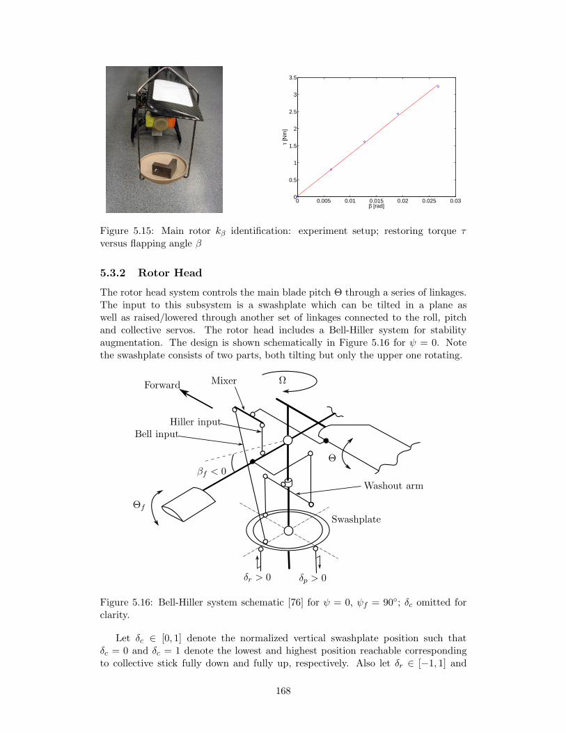
0 0.005 0.01 0.015 0.02 0.025 0.030
0.5
1
1.5
2
2.5
3
3.5
β [rad]
τ [N
m]
Figure 5.15: Main rotor kβ identification: experiment setup; restoring torque τversus flapping angle β
5.3.2 Rotor Head
The rotor head system controls the main blade pitch Θ through a series of linkages.The input to this subsystem is a swashplate which can be tilted in a plane aswell as raised/lowered through another set of linkages connected to the roll, pitchand collective servos. The rotor head includes a Bell-Hiller system for stabilityaugmentation. The design is shown schematically in Figure 5.16 for ψ = 0. Notethe swashplate consists of two parts, both tilting but only the upper one rotating.
Forward Mixer
Bell inputHiller input
Washout arm
Swashplate
δp > 0δr > 0
Ω
Θf
Θ
βf < 0
Figure 5.16: Bell-Hiller system schematic [76] for ψ = 0, ψf = 90; δc omitted forclarity.
Let δc ∈ [0, 1] denote the normalized vertical swashplate position such thatδc = 0 and δc = 1 denote the lowest and highest position reachable correspondingto collective stick fully down and fully up, respectively. Also let δr ∈ [−1, 1] and
168

δp ∈ [−1, 1] denote the normalized swashplate tilt about the helicopter roll and pitchaxes, respectively. The sign convention is shown in Figure 5.16 with δr = 0, δp = 0denoting the swashplate is level in the roll and pitch axis or the roll and pitch sticksare centered, respectively. The limits δr = −1 and δr = 1 represent maximum leftand right swashplate tilt or roll stick fully left and fully right, respectively. Similarlyδp = −1 and δp = 1 represent maximum forward and backward swashplate tilt orpitch stick fully front and fully back, respectively. Using δc, δr and δp as inputsallows the math model to handle different types of swashplate layouts, e.g. the 90
control setup on the Bergen Industrial Twin or a 120 CCPM control used on theMini-Titan electric heli; the mapping from δ to servo commands will be discussedin Section 5.3.5.
The Bell-Hiller system consists of a flybar with small airfoils attached to its ends,mounted at 90 to the main blades and rotating about a teetering hinge inside themain rotor shaft. The washout arm moves together with the swashplate such thatthe input δc does not affect the pitch Θf of the flybar airfoils but only the collectivecomponent of the main rotor blade pitch Θ (5.22):
A0 = Ccδc +Dc (5.41)
where Cc and Dc are constants which depend on the mechanical link setup and pilotsettings on the transmitter. Physically these are identified by moving the collectivestick from δc = 0 to δc = 1 and measuring the range of Θ and its value at δc = 0,respectively, with Dc < 0 being typical. The flybar pitch Θf is a periodic functionof the swashplate tilt as
Θf = (KHδr) cosψf + (KHδp) sinψf (5.42)
where KH is the Hiller input ratio of flybar cyclic pitch amplitude to swashplate tilt;remark the flybar paddle with pitch Θf shown in Figure 5.16 is at azimuth stationψf = 90. The 2π-periodic flybar pitch function (5.42) will cause the flybar to flapwith the approximate profile
βf (t, ψ) ≈ −a1f (t) cosψf + b1f (t) sinψf (5.43)
where the sign convention has been chosen identical to (5.30). The dynamics ofa1f and b1f will be analyzed in Section 5.3.2.1; remark that (5.43) has no coningcomponent because the flybar is a teetering rotor. Using the Mixer arm shownin Figure 5.16 the cyclic amplitudes A1, B1 of the main rotor pitch (5.22) Θ =A0+A1 cosψ+B1 sinψ are controlled by a mix of swashplate tilt and flybar flappingangles as
A1 = KBδr +KF b1f
B1 = KBδp +KFa1f(5.44)
where KB is the Bell input ratio of main rotor cyclic pitch amplitude to swashplatetilt, and KF is known as the flybar ratio4 of main rotor pitch to flybar flappingangle. The three ratios above are functions of mechanical linkage setup.
The Bell and Hiller input ratios KB and KH can be measured as follows: tiltthe swashplate by moving the roll or pitch transmitter stick to one of its limits and
4This is standard terminology in RC helicopters. Typical flybar ratios range from .5 : 1 to 1 : 1;this is further discussed at the end of Section 5.3.2.1
169

hold it there. Using a pitch gauge measure max(Θ), min(Θ) as well as max(Θf ),min(Θf ) over a complete 360 main rotor revolution; the input ratios are then givenby
KB =max(Θ)−min(Θ)
2, KH =
max(Θf )−min(Θf )
2
Remark this assumes the roll or pitch stick center position δ = 0 corresponds toa perfectly level swashplate, and so it is important to zero out any trims on thesesticks for this procedure.
The flybar ratio KF is computed by tilting the flybar to a given angle βf withrespect to the horizontal and measuring the resulting main rotor blade pitch Θ usinga pitch gauge. The experimental setup is shown in Figure 5.17; the tilt angle βf ismeasured using a digital inclinometer. We obtain a set of (βf ,Θ) pairs which areplotted to obtain KF as the slope of least-squares linear fit to the data, also shownin Figure 5.17. Computing the slope of the line we find KF = 0.66 i.e. a flybar ratioof .66 : 1.
−15 −10 −5 0 5 10 15
−10
−6
−2
2
6
10
βf [deg]
Θ [d
eg]
Figure 5.17: Flybar ratio KF identification: experiment setup; blade pitch Θ versusflybar tilt βf
5.3.2.1 Flybar Flapping Dynamics
A schematic of the flybar is shown in Figure 5.18. The flybar consists of a uniformrod hinged at the center of the main rotor with two paddle airfoils attached to itsends. The flybar is free to teeter about its pivot and its flapping angle βf is measuredupwards from the horizontal plane. The ijk frame is fixed to the flybar’s centreof mass so the moment balance is governed by the standard Euler equation (5.10)rather than its “extended” version (5.18) which was employed in Section 5.3.1.3. Theouter radius of the flybar is denoted Rf and the radial distance to each paddle’sinner edge is εfRf where by construction 0 < εf < 1.
The flybar paddles are symmetric however they are tapered in shape, have asharp leading edge and their maximum thickness occurs at the midpoint xf/cf = 0.5.The average paddle chord is cf = 50 mm and maximum thickness is tf = 4.4 mmsuch that tf/cf = 0.09. The paddle is classified as the modified four-digit airfoil [8,p. 117] NACA 0009-05, where the first four digits function as before, the fifth digitindicates relative magnitude of the leading edge radius with 0 denoting a sharp edge(a 6 denotes the standard curvature of NACA four-digit series airfoils), and thesixth digit indicates the maximum thickness position with 5 indicating mid-chord.
170

i
j
k
u
vw
p
q
Ω
RfεfRf
ψf
βf
Figure 5.18: Flybar Kinematics
This geometry is used in JavaFoil to compute the paddle lift curve slope af usingReynolds number (5.20) with Vf = ΩRf .
Denoting the flybar’s angular velocity vector as [pf qf rf ]T , the dynamics ofβf are obtained from a moment balance about the j axis (5.11)
Jfyy qf + pfrf (Jfxx − Jfzz) =Mf
where Mf is the net external moment about the j axis. The flybar is modeledas a slender rod of mass mr and length 2Rf with point masses mp on each endrepresenting the paddles where by direct measurementmr = 0.043 kg, Rf = 0.306 mand mp = 0.025 kg. Using the CM-fixed frame illustrated in Figure 5.18 we haveby [100, p. 713]
Jfxx ≈ 0
Jfyy =1
12mr(2R
2f ) + 2mpR
2f
Jfzz =1
12mr(2R
2f ) + 2mpR
2f = Jfyy
and thus Jfxx − Jfzz = −Jfyy := −Jf and the previous equation above becomes
Jf (qf − pfrf ) =Mf (5.45)
The angular velocity components in (5.45) can be obtained by inspection of Fig-ure 5.18:
pf = −p cosψf cos βf − q sinψf cos βf − Ω sin βf
qf = p sinψf − q cosψf + βf
rf = −p cosψf sin βf − q sinψf sin βf +Ωcos βf
which is exactly analogous to the main blade flapping analysis in Section 5.3.1.3 dueto ψf being measured from the same datum as ψ. We directly compute
qf = p sinψf + pΩcosψf − q cosψf + qΩ sinψf + βf
and substituting the above into (5.45) then using the small-angle approximationscos βf ≈ 1, sin βf ≈ βf , β
2f ≈ 0 as well as p2 ≈ 0, q2 ≈ 0, pq ≈ 0 due to p, q ≪ Ω we
171

get
pfrf = −pΩcosψf − qΩ sinψf −Ω2βf ,
Jf (qf − pfrf ) = Jf
(βf + p sinψf − q cosψf + 2pΩcosψf + 2qΩ sinψf +Ω2βf
)
(5.46)
which is analogous to (5.26). The moment about the central hinge Mf in (5.45)comes only from aerodynamic lift, due to the weight moment canceling itself outon the two sides and the absence of a restoring spring term. The tangential andperpendicular flow components UT , UP on the advancing paddle at distance l fromthe central hinge are obtained by inspection of Figure 5.18 or by analogy from (5.27):
UaT = Ωl cos βf + u sinψf − v cosψf
UaP = (vi − w) cos βf + u sin βf cosψf + v sin βf sinψf + βf l + pl sinψf − ql cosψf
On the retreating paddle, ψrf = ψf + π hence sinψrf = − sinψf , cosψrf = − cosψf
and βrf = −βf , βrf = −βf , βrf = −βf :
U rT = Ωl cos βf − u sinψf + v cosψf
U rP = (vi − w) cos βf + u sin βf cosψf + v sin βf sinψf − βf l − pl sinψf + ql cosψf
From (5.42) the advancing paddle’s pitch angle is the period function
Θf = (KHδr) cosψf + (KHδp) sinψf := Af cosψf +Bf sinψf
and it follows the retreating paddle has the pitch angle
Θrf = −Af cosψf −Bf sinψf = −Θf
As in Section 5.3.1.3 the moment created by aerodynamic lift on the advancingpaddle is
Ma(ψf ) =
∫ Rf
εfRf
ldF⊥ =ρafcf2
∫ Rf
εfRf
l[Θf (U
aT )
2 − UaTUaP
]dl
The retreating paddle creates the moment
M r(ψf ) = −∫ Rf
εfRf
ldF⊥,r = −ρafcf2
∫ Rf
εfRf
l[−Θf (U
rT )
2 − U rTUrP
]dl
where the −1 factor is due to positive (upwards) lift on the retreating paddle creatinga negative contribution to Mf . The total aerodynamic lift moment Mf =Ma+M r
is then
Mf =1
2ρaf cf
∫ Rf
εfRf
l
(Af cosψf +Bf sinψf )
[(UaT )
2 + (U rT )2]−UaTU
aP +U rTU
rP
dl
which evaluates to
Mf =1
4ρaf cfR
2f (1− ε2f )
[u2 + v2 + (1 + ε2f )(RfΩ)
2 − (u2 − v2) cos 2ψf
− 2uv sin 2ψf
](Af cosψf +Bf sinψf ) +
[2v(vi − w) + q(1 + ε2f )R
2fΩ]cosψf
+ 2uvβf cos 2ψf −[2u(vi − w) + p(1 + ε2f )R
2fΩ]sinψf
− (u2 − v2)βf sin 2ψf − (1 + ε2f )R2fΩβf
172

and which is substituted into (5.45) along with (5.46) to yield
βf +
ρafcfR
4f (1− ε4f )Ω
4Jf
βf +
Ω2 +
ρaf cfR2f (1− ε2f )
4Jf
[(u2 − v2) sin 2ψf
− 2uv cos 2ψf
]βf = −p sinψf + q cosψf − 2pΩcosψf − 2qΩ sinψf
+ρafcfR
2f (1− ε2f )
4Jf
[u2 + v2 + (1 + ε2f )(RfΩ)
2 − (u2 − v2) cos 2ψf
− 2uv sin 2ψf
](Af cosψf +Bf sinψf ) +
[2v(vi − w) + q(1 + ε2f )R
2fΩ]cosψf
−[2u(vi − w) + p(1 + ε2f )R
2fΩ]sinψf
(5.47)The coefficient group ρaf cfR
4f (1− ε4f )/Jf in (5.47) is similar to the Lock number γ
introduced in Section 5.3.1.3. Let Jf = 2Jβf where Jβf measures the mass momentof inertia of one-half of the flybar about its flapping hinge5. The term R4
f (1− ε4f ) =
R4f − (εfRf )
4 measures the length of the half-flybar’s lifting surface i.e. the widthof an individual paddle. We thus define the flybar Lock number
γf :=ρaf cfR
4f (1− ε4f )
Jβf
which is introduced into (5.47). The assumed flybar flapping profile (5.43) is differ-entiated twice w.r.t. time giving
βf = −a1f cosψf + b1f sinψf
βf = (−a1f + b1fΩ) cosψf + (a1fΩ+ b1f ) sinψf
βf = (−a1f + a1fΩ2 + 2b1fΩ) cosψf + (2a1fΩ+ b1f − b1fΩ
2) sinψf
(5.48)
analogously to (5.31) and (5.32). Substituting the above into (5.47) and matchingcoefficients of cosψf and sinψf gives a set of coupled second-order linear differentialequations for the flapping angles a1f and b1f . As in Section 5.3.1.3 we pre-simplifyby numerically computing γf = 0.93 using the identified values listed in Section 5.5.Since γf < γ is very small, we are able to disregard the translational velocity effectsby setting u = v = 0 in (5.47) which simplifies to
βf +γfΩ
8βf +Ω2βf =− p sinψf + q cosψf − 2pΩcosψf − 2qΩ sinψf
+γfΩ
2
8(Af cosψf +Bf sinψf ) +
γfΩ
8(q cosψf − p sinψf )
Substituting (5.48) into the above and matching coefficients of cosψf and sinψf
5This by analogy to Jβ in Section 5.3.1.3 which measures the mass moment of inertia of a singleblade about its flapping axis
173
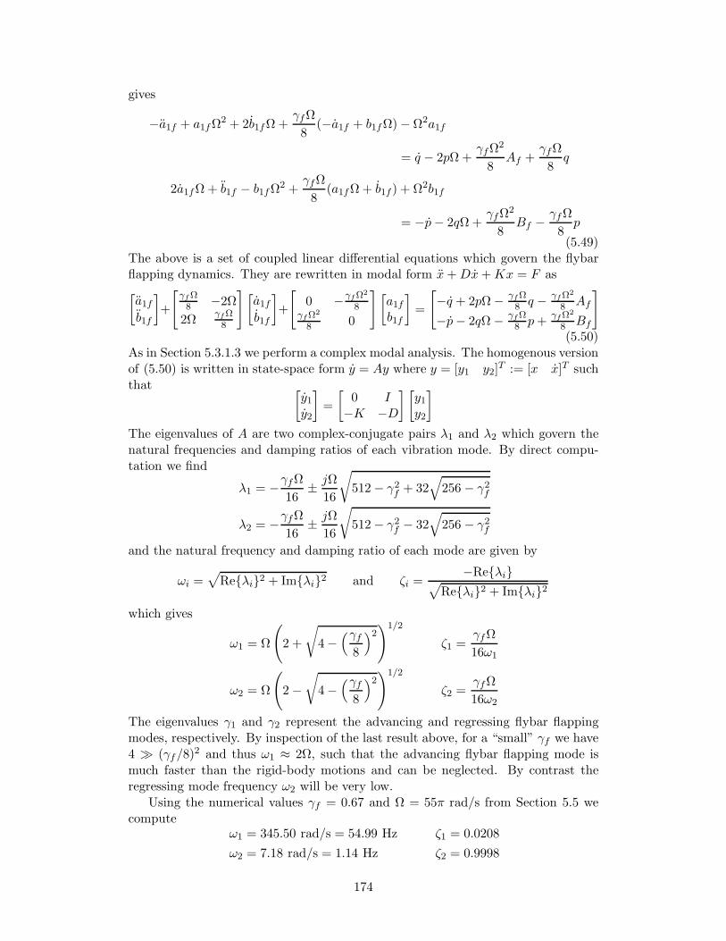
gives
−a1f + a1fΩ2 + 2b1fΩ+
γfΩ
8(−a1f + b1fΩ)− Ω2a1f
= q − 2pΩ+γfΩ
2
8Af +
γfΩ
8q
2a1fΩ+ b1f − b1fΩ2 +
γfΩ
8(a1fΩ+ b1f ) + Ω2b1f
= −p− 2qΩ+γfΩ
2
8Bf −
γfΩ
8p
(5.49)The above is a set of coupled linear differential equations which govern the flybarflapping dynamics. They are rewritten in modal form x+Dx+Kx = F as
[a1fb1f
]+
[γfΩ8 −2Ω
2ΩγfΩ8
][a1fb1f
]+
[0 −γfΩ
2
8γfΩ
2
8 0
][a1fb1f
]=
[−q + 2pΩ− γfΩ
8 q − γfΩ2
8 Af
−p− 2qΩ − γfΩ8 p+
γfΩ2
8 Bf
]
(5.50)As in Section 5.3.1.3 we perform a complex modal analysis. The homogenous versionof (5.50) is written in state-space form y = Ay where y = [y1 y2]
T := [x x]T suchthat [
y1y2
]=
[0 I
−K −D
] [y1y2
]
The eigenvalues of A are two complex-conjugate pairs λ1 and λ2 which govern thenatural frequencies and damping ratios of each vibration mode. By direct compu-tation we find
λ1 = −γfΩ16
± jΩ
16
√512− γ2f + 32
√256 − γ2f
λ2 = −γfΩ16
± jΩ
16
√512− γ2f − 32
√256 − γ2f
and the natural frequency and damping ratio of each mode are given by
ωi =√
Reλi2 + Imλi2 and ζi =−Reλi√
Reλi2 + Imλi2
which gives
ω1 = Ω
(2 +
√4−
(γf8
)2)1/2
ζ1 =γfΩ
16ω1
ω2 = Ω
(2−
√4−
(γf8
)2)1/2
ζ2 =γfΩ
16ω2
The eigenvalues γ1 and γ2 represent the advancing and regressing flybar flappingmodes, respectively. By inspection of the last result above, for a “small” γf we have4 ≫ (γf/8)
2 and thus ω1 ≈ 2Ω, such that the advancing flybar flapping mode ismuch faster than the rigid-body motions and can be neglected. By contrast theregressing mode frequency ω2 will be very low.
Using the numerical values γf = 0.67 and Ω = 55π rad/s from Section 5.5 wecompute
ω1 = 345.50 rad/s = 54.99 Hz ζ1 = 0.0208
ω2 = 7.18 rad/s = 1.14 Hz ζ2 = 0.9998
174

which confirms the regressing flybar flapping mode’s natural frequency is sufficientlylow, or equivalently the 5% step input settling time ts = 3/(ζ2ω2) = 0.418 s issufficiently long to noticeably impact the helicopter’s dynamics. The regressingmode’s near-critical damping ratio means it can be approximated as a first-ordersystem by setting a1f = b1f = 0 in (5.49) as well as setting p = q = 0 exactly as inSection 5.3.1.3. The regressing flapping dynamics of the flybar become
2b1fΩ+γfΩ
8(−a1f + b1fΩ) = −2pΩ+
γfΩ2
8Af +
γfΩ
8q
2a1fΩ+γfΩ
8(a1fΩ+ b1f ) = −2qΩ+
γfΩ2
8Bf −
γfΩ
8p
We assume the control links from the swashplate to the flybar are phased to decouplethe flapping response, i.e. the roll cyclic Af = KHδr affects only the lateral flappingb1f and the pitch cyclic Bf = KHδp only the longitudinal flapping a1f . This isdone by dropping respectively a1f and b1f from the first and second equation above.Normalizing the coefficients of Af and Bf gives
16
γfΩa1f + a1f = − 16
γfΩq − 1
Ωp+Bf
16
γfΩb1f + b1f = − 16
γfΩp+
1
Ωq +Af
where Bf = KHδp and Af = KHδr are inputs from the swashplate. Finally, eval-uating the coefficients 16/(γfΩ) = 0.1392 and (1/Ω) = 0.0058 we see the on-axiseffect of q on a1f and p on b1f dominate the off-axis effects and the above can besimplified to
16
γfΩa1f + a1f = − 16
γfΩq +KHδp
16
γfΩb1f + b1f = − 16
γfΩp+KHδr
(5.51)
where 16/(γfΩ) := τf is the time constant of the simplified flybar flapping dynam-ics (5.51).
As discussed in Section 5.3.2 the flybar flapping angles enter the main rotorcyclic pitch amplitudes A1, B1 as (5.44)
A1 = KBδr +KF b1f
B1 = KBδp +KFa1f
and A1 and B1 in turn map to main rotor flapping angles by (5.36)
b1 = A1
a1 = B1
This last relationship was obtained in Section 5.3.1.4 by neglecting the main rotorflapping dynamics due to their fast time constant. The flybar performs two func-tions: first, it slows down the main rotor flapping response to swashplate tilt sinceδp → a1f → B1 → a1 and δr → b1f → A1 → b1 provide a partial rate limit on a1 andb1 due to the first-order dynamics of a1f and b1f . Second, the flybar dynamics (5.51)
175

contain negative feedback terms −τfq and −τfp which provide derivative action inthe pitch and roll channels of the helicopter which damps the response to externaldisturbances such as wind gusts.
The flybar can be summarized in control diagram form as shown in Figure 5.19for the roll channel; the pitch channel has the same diagram with (δr, b1f , A1, b1, p)replaced by (δp, a1f , B1, a1, q). The Roll Dynamics block represents p = qr(Jyy −Jzz)/Jxx + L/Jxx from (5.11) where L ≈ Lhmr = (hmrT
hmr + kβ)b1, i.e. we use
the roll moment expression in hover developed in Section 5.3.1.5 instead of L =hmrYmr + Lmr due to the complexity of the Ymr and Lmr expressions; the keypoint of this block is that a b1 > 0 rotor disc tilt provides a p > 0 roll response.Increasing the flybar ratio KF increases the derivative feedback action, making thehelicopter more resistant to disturbances such as wind gusts but also slowing downinput step responses; indeed higher flybar ratios are better for beginning pilotsas well as helicopter competitions which demand stable hover and resistance towind conditions, while lower flybar ratios are better for 3D flying which requirevery nimble handling of the helicopter. The derivative feedback action can also beboosted by increasing τf = 16/(γfΩ) which by the definition of γf is equivalentto reducing af , cf , Rf and augmenting εf , Jβf . This is why using heavier, shorterpaddles makes the helicopter more stable, while using longer flybars with lightweight,wide paddles (whose larger aspect ratio (Rf − εfRf )/c provides higher a values) ispreferred for 3D flight.
KH KF 1
τf
KB
Roll
Dynamicsτf b1f + b1f = u
+
−
++δr b1f A1 b1
p
Figure 5.19: Rotor head system diagram — roll channel
5.3.3 Tail Rotor
The tail rotor uses a fixed-pitch design, similar to an airplane propeller. We usethe tail blade pitch Θt as the input term as in Section 5.3.1.5. Due to the fixedpitch design the tail rotor does not exhibit flapping. The tail rotor is geared torotate counter-clockwise as viewed from the right side of the helicopter at the rateΩt = KtΩ where Kt > 1 is the tail to main rotor gearing ratio. We define Θt > 0as the pitch which creates tail rotor thrust Ttr in the positive yb direction and takethe tail blade azimuth position ψt = 0 as the blade’s rear-most position. This isillustrated in Figure 5.20. The tail rotor blades are symmetric with ct = 32.5 mmand maximum thickness tt = 3.9 mm at xt = 10 mm from the leading edge, givingtt/ct = 0.12, xt/ct = 0.31 which classifies them as NACA 0012 airfoils. We obtainat, CD,t as in Section 5.3.1.2 using Vt = ΩtRt (where Rt is the tail rotor disc radius)to compute the Reynolds number (5.20).
176

Ωt
ψt
dtr
htr
Qtr
u
vw
p
qr
dtr
vi,t
Ttr
Figure 5.20: Helicopter tail: Side view (left), Overhead view (right)
By inspection of Figure 5.20, the tail blade airfoil section at distance l from therotor shaft is subject to tangential and perpendicular flow components
UT = Ωtl + u sinψt + w cosψt + q(dtr + l cosψt)
UP = vi,t + v + p(htr − l sinψt)− r(dtr + l cosψt)
where dtr and htr are the longitudinal distance and height of the tail rotor axisw.r.t. the helicopter’s CM. The tail rotor induced velocity vi,t is assumed constantacross the rotor disc as in Section 5.3.1. Using (5.21) in Section 5.3.1.2 the infinites-imal force components perpendicular and parallel to the vertical plane are
dF⊥ =1
2ρatct
(ΘtU
2T − UTUP
)dl
dF ‖ =1
2ρatct
(ΘUTUP − U2
P
)dl +
1
2ρctCD,tU
2Tdl
The tail rotor thrust and counter-torque are evaluated from
Ttr =Nbt
2π
∫ 2π
0
∫ Rt
0dF⊥ dψt
Qtr =Nbt
2π
∫ 2π
0
∫ Rt
0l dF ‖ dψt
where Nbt = 2 is the number of tail rotor blades. The in-plane forces Xtr, Ytr andmoments Ltr, Mtr are neglected as small, which is justified due to the size of thetail rotor as compared to the main one. The Ttr expression evaluates to
Ttr =ρatctRtNbt
24
[4(RtΩt)
2 + 6(u2 + w2) + 6qRt(w + 2dtrΩt)
+ 2q2(R2t + 6d2tr)
]Θt + 2qrR2
t + 3Rt(pu+ rw)
− 6(RtΩt + 2qdtr)(v + vi,t + phtr − rdtr)
(5.52)
The tail rotor induced velocity vi,t is computed as in Section 5.3.1.1. We assume themain rotor’s downwash is sufficiently far to not affect the tail rotor inflow due to the
177

Bergen Industrial Twin’s extended tail boom (c.f. Figure 5.23 in Section 5.3.7.1).Note that for a smaller helicopter where the rotor disc overhangs the tail this as-sumption would not hold, e.g. [59, p. 49]. Since the tail rotor disc is vertical, thegeneral flight inflow equation (5.19) becomes
vi,t =Ttr
2ρπR2t
√u2 + (w + qdtr)2 + (v + phtr − rdtr + vi,t)2
which gives a transcendental equation for Ttr when substituted into (5.52), just asfor the main rotor in Section 5.3.1.5. At hover, the tail thrust (5.52) reduces to
T htr =ρatctRtNbt
12
2(RtΩt)
2Θt − 3RtΩtvhi,t
(5.53)
where
vhi,t =
√T htr
2ρπR2t
(5.54)
We obtain an explicit T htr = T htr(Θt) expression by substituting (5.54) into (5.53)and solving a quadratic equation as in Section 5.3.1.5. The substitution gives
T htr =ρatctR
3tNbtΩ
2t
6Θt −
actRtNbtΩt√ρ
4√2π
√T htr := CTtrΘt −DT
tr
√T htr
with CTtr, DTtr positive constants. The solution to the above is exactly analogous
to (5.39)
T htr = CTtrΘt +(DT
tr)2
2−DT
tr
√CTtrΘt +
(DTtr)
2
4(5.55)
where we have chosen the solution for which Θt = 0 =⇒ T htr = 0. A simpler versionof (5.55) can be obtained by employing T htr = Qhmr/dtr ≈ CQmr(mg)3/2 + DQ
mr in(5.53) which gives
T htr ≈ CTtrΘt −(DTtr
√CQmr(mg)3/2 +DQ
mr
)
but which requires w = r = 0, i.e. zero heave acceleration and zero yaw angularacceleration, making it much worse than (5.55).
Returning above, the Qtr expression is
Qtr = −ρatctR2tNbt
48
[3qrR2
t + 4Rt(pu+ rw)− 4(2RtΩt + 3qdtr)
(v + vi,t + phtr − rdtr)]Θt + 3(p2 + r2)R2
t + 12(v + vi,t + phtr − rdtr)2
+ρctR
2tCD,tNbt
48
6(RtΩt)
2 + 6(u2 + w2) + 8qRt(w + 2dtrΩ) + 3q2(R2t + 4d2tr)
178

and at hover this simplifies to
Qhtr = −ρatctR2tNbt
48
[− 4(2RtΩt)v
hi,t
]Θt + 12(vhi,t)
2
+ρctR
2tCD,tNbt
48
6(RtΩt)
2
=ρatctR
2tNbtv
hi,t
24RtΩt
4(RtΩt)
2Θt − 6RtΩtvhi,t
+ρctR
4tΩ
2tCD,tNbt
8
=T htrRtRtΩt
√T htr
2ρπR2t
+ρctR
4tΩ
2tCD,tNbt
8:= CQtr
(T htr
)3/2+DQ
tr (5.56)
where by inspection CQtr and DQtr are constants.
5.3.3.1 Tail Rotor Contributions
The tail rotor’s thrust and counter-torque Ttr and Qtr generate the following forceand moment components along the helicopter’s body-fixed axes:
Xtr = 0
Ytr = Ttr
Ztr = 0
Ltr = htrTtr
Mtr = −QtrNtr = −dtrTtr
where htr and dtr are the height and longitudinal distance, respectively, of the tailrotor hub w.r.t. the center of mass as illustrated in Figure 5.20; as in Section 5.3.1.6these are directly measured c.f. Figure 5.3 in Section 5.2. In hover this becomes
Xhtr = 0
Y htr = T htr
Zhtr = 0
Lhtr = htrThtr
Mhtr = −CQtr
(T htr
)3/2−DQ
tr
Nhtr = −dtrT htr
where by (5.55)
T htr = CTtrΘt +(DT
tr)2
2−DT
tr
√CTtrΘt +
(DTtr)
2
4
and where
CTtr :=ρatctR
3tNbt(KtΩ)
2
6DTtr :=
actRtNbtKtΩ√ρ
4√2π
CQtr :=1
RtKtΩ√2ρπ
DQtr :=
ρctR4tNbtCD,t(KtΩ)
2
8
179

5.3.3.2 Tail Gyro
As seen in Section 5.3.1.5 the main rotor’s counter-torque on the helicopter body
Qmr is a function of thrust Tmr, e.g. Qhmr = CQmr
(T hmr
)3/2+DQ
mr in hover, such thatchanges in collective input require adjustments to the tail input in order to cancelthe counter-torque. On full-sized helicopters this is done manually by the pilot byadjusting the tail pedal inputs [121, p. 43]. RC helicopters such as the BergenIndustrial Twin have relatively small Jzz mass moment of inertias and high thrust-to-weight ratios, which make manual compensation of counter-torque too taxing forthe pilot. For this reason tail rotor control is augmented with an electronic gyrowhich provides closed-loop control of the tail input using the sensed yaw rate r.
The ANCL helicopter employs the popular Futaba GY401 tail gyro [58] whichprovides two modes of operation: a Normal mode which stabilizes the sensed yawrate r using the tail pitch servo and thus provides damping in the yaw channel; and aHeading Hold6 mode which provides tracking control of r using tail stick deflectionsfor rref and a PI control action on the error signal. For zero tail stick deflection,Heading Hold mode can thus maintain a steady heading angle ψ in the presenceof exogenous inputs (changes in Qmr, wind gusts), while Normal mode will removeyaw velocity r but exhibit a steady-state error in ψ. The GY401 manual [58] callsthis the weathervane effect, where a helicopter hovering in wind under Normal modewill eventually align itself along the wind vector due to its tail stabilizers, whereasin the same situation Heading Hold mode is able to maintain a prescribed headingangle.
The GY401 unit uses two inputs from the on-board receiver, the tail channel andgyro sensitivity channel, and one output to the tail servo which directly controls theblade pitch Θt used in Section 5.3.3. In Normal mode, the tail input is added to again on the sensed r and passed directly to the tail servo, whereas in Heading Holdmode this input is used as rref where rref = 0 is taken as the tail input level atinitialization. The gyro sensitivity input is interpreted as follows: for a “neutral”signal from the receiver (PWM with TON = 1.5 ms, c.f. Section 5.3.5) the gyro gainis set to zero. For PWM signals above neutral i.e. 1.5 ms < TON < 2.0 ms thegyro operates in Heading Hold mode with the P and I gain values increasing from0 to 100% of their maximum values. Conversely for signals below neutral the gyrooperates in Normal mode with 1.5 ms > TON > 1.0 ms mapping to a P gain from0 to 100% of its maximum value. In this way the GY401 can be switched in-flightbetween Normal and Heading Hold modes, and the feedback gains adjusted to fine-tune the overall performance. Heading Hold mode is useful for hovering and forwardflight while Normal mode is better for turns as well as certain 3D maneuvers.
The exact relationship between gyro sensitivity input and gain values in Normaland Heading Hold modes is not available from Futaba and thus requires experimentalidentification. The GY401 contains a “Control Delay” trimmer whose setting isadjustable from 0 to 100%. The exact function of this feature is not explainedalthough we speculate it acts as a rate limit on the output control signal to the tailservo; this must be confirmed in experiment and the exact relationship between thissetting and resulting rate limit needs to be identified. Heading Hold mode appearsto implement an integrator reset function, although this is not stated in the manual,
6Futaba calls this the Angular Vector Control System (AVCS) mode
180

and the reset error threshold requires experimental identification as well.Based on the above paragraph we can model the tail gyro unit in one of the
following ways, listed in order of increasing difficulty:
1. Use Heading Hold mode and assume the input sensitivity is properly tunedsuch that the yaw channel is stabilized and r = rref , i.e. discard the r dynam-ics.
2. Turn off the tail gyro by setting the gyro sensitivity input to neutral (TON =1.5 ms). The r dynamics remain and Qmr, Ttr terms are computed as inSections 5.3.1.5 and 5.3.3, respectively.
3. Include an identified model of the tail gyro as in e.g. [22].
Define δt ∈ [−1, 1] as the normalized tail input where δt = −1 denotes tail stickfully left and δt = 1 fully right. The map from δt to the helicopter model has threepossible forms corresponding to the above:
1. r = rref = κtδt where κt is identified in flight by commanding a maximum tailstick deflection and measuring the resulting yaw rate rmax using the avionicsbox, such that κt = |rmax|.
2. Θt = Ctδt +Dt where Ct = [Θt(δt = 1)−Θt(δt = −1)]/2, Dt = Θt(δt = 0) aremeasured using a pitch gauge7. We have Ct,Dt < 0 because a positive yawturn (δt > 0) requires Θt < 0 by sign convention of Section 5.3.3.
3. rref = κtδt as in 1, then compute er = rref − r and Θt = κP er+κI∫er where
κP , κI are the identified gains of the tail gyro; also include the “control delay”and integrator reset into the calculation.
For option 1, Ttr still appears in the Ytr and Ltr terms summarized in Section 5.3.3.1and must be computed from
Ttr = −Qmrdtrwhere Qmr is given in Section 5.3.1.5 and Ttr < 0 compensates for Qmr > 0 by signconvention in Section 5.3.3.
5.3.4 Rotor Speed and Engine
The dynamics of Ω are governed by a moment balance on the main rotor shaft,
Ω = r +1
Jmr(KeQe −Qmr −KtQtr),
where Jmr is the rotational inertia of the main blades and rotor head, Ke > 1 is theengine to main rotor gearing ratio, Qe is the torque generated by the engine, Qmr,Qtr are the counter-torques from the main and tail rotors available respectively fromSections 5.3.1.5 and 5.3.3, and Kt > 1 is the tail to main rotor gearing ratio. Theengine input is a fuel throttle controlled by a dedicated servo. Let δe ∈ [0, 1] denotethe normalized fuel throttle input with δe = 0 and δe = 1 denoting fully closed and
7The Θt offset term Dt models the design of the tail servo linkage.
181

fully open fuel inputs, respectively. Following [59, p. 44] we model the engine outputpower Pe and subsequently output torque as
Pe = Pmaxe δe =⇒ Qe =PeKeΩ
where Pmaxe is the engine’s maximum output power. The δe to Qe model is as-sumed instantaneous since the time constants associated to fuel flow, air intake andcombustion are much faster than the vehicle’s dynamics [59, p. 44].
Internal combustion engines operate most efficiently in a narrow RPM band,hence maintaining a constant Ω is desirable. This is accomplished using eitheran engine governor, which maintains a target Ω by controlling δe using a PI con-trol structure, or through a throttle-pitch curve, a nonlinear map from δc to δeprogrammed on the RC transmitter and tuned by the pilot. The current ANCLhelicopter uses the latter solution, with two different versions of the curve usedfor no-payload (“stock”) and full-payload flights. For illustration purposes the twocurves are plotted in Figure 5.21; the values come from a lookup table, which iseither built from servo inputs logged by the on-board avionics box or downloadeddirectly from the transmitter’s flash memory card.
0 0.1 0.2 0.3 0.4 0.5 0.6 0.7 0.8 0.9 10
0.1
0.2
0.3
0.4
0.5
0.6
0.7
0.8
0.9
1
δc
δ e
0 0.1 0.2 0.3 0.4 0.5 0.6 0.7 0.8 0.9 10
0.1
0.2
0.3
0.4
0.5
0.6
0.7
0.8
0.9
1
δc
δ e
Figure 5.21: Throttle-pitch curves: Stock (left), Full-payload (right)
Based on the above discussion, we will ignore rotor speed dynamics and take Ωas constant, assuming a well-tuned curve or by physically adding a governor to thehelicopter. The dynamics of Ω are important in autorotations [4]; in this case, theengine and tail rotors are disengaged through a centrifugal clutch, such that Ω is afunction of Qmr only.
5.3.5 Servo Commands
The swashplate normalized vertical position δc and tilt angles δr, δp introducedin Section 5.3.2 are physically controlled by the collective, roll and pitch servosthrough a set of mechanical linkages. Similarly the tail rotor pitch Θt in Section 5.3.3and the fuel throttle in Section 5.3.4 are controlled by their corresponding servos.The servos themselves are controlled by PWM signals coming from either the on-board Futaba R149DP radio receiver or generated by the avionics’s MeasurementComputing CTR10HD card, except for the tail servo which is controlled by PWMsignals generated by the tail gyro unit as discussed in Section 5.3.3.2.
182

The servo reacts by rotating an output wheel, where the output rotation ismechanically limited to a [−45, 45] range where 0 is the servo’s neutral position.The input PWM signal to the servo is a square wave with period TPWM = 1/70 s ≈14.3 ms and pulse width of TON where pulse widths of TON = 1.0 ms, TON = 1.5 msand TON = 2.0 ms command output rotations of −45, 0 and 45, respectively [75,p. 11]. The same signal type is used for the inputs to the tail gyro discussed inSection 5.3.3.2 where the above pulse widths are interpreted as “min”, “neutral”and “max” signals, respectively.
The PWM duty cycle ∆ is defined as
∆ =TON
TPWM
such that for TPWM = 1/70 s we have ∆ = 70TON and 0.070 ≤ ∆ ≤ 0.140 for theabove servo logic. The duty cycle ∆ is the numerical value either logged or outputby the avionics box via its CTR10HD card. For instance generating a “neutral”signal on the gyro sensitivity channel (c.f. Section 5.3.3.2) corresponds to setting∆ = 0.105 on the appropriate CTR10HD PWM output channel.
Since the servo output rotations are converted to linear motion by a set of me-chanical linkages, the full [−45, 45] output range is typically not used, and in factthe extreme ranges may cause jamming or breaking of the linkages. For this reasonthe normalized system inputs δ are used, which respect the servo limits programmedby the pilot into the transmitter unit. We then need to identify the mapping fromδ to ∆, such that the avionics box can mimic the signal limits programmed into thetransmitter.
The identification process is made using the avionics box’s receiver logging func-tionality. For collective, roll, pitch and tail inputs we propose the linear maps
∆c = mcδc + bc
∆r = mrδr + br
∆p = mpδp + bp
∆t = mtδt + bt
(5.57)
wherems = ∆δs=1 −∆δs=0
bs = ∆δs=0
s = c, r, p, t
The identified values of the m and b parameters in (5.57) are listed in Section 5.5.The duty cycles were logged using the “Bergen-02” transmitter programming em-ployed for full-payload flight, c.f. Section 5.3.4; sample plots for the collective androll channels are shown in Figure 5.22 where the corresponding pilot sticks are sweptthrough their full range of motion. Observe that the collective duty uses a largerportion of its maximum 0.070 ≤ ∆c ≤ 0.140 range than does ∆r. As expected theroll stick neutral position δr = 0 provides a duty of ∆r ≈ 0.105 corresponding toneutral servo output. We identify mc < 0 and mr < 0 from the plots due to themechanical linkage setup between servo output wheel and swashplate.
The ∆e duty cycle input to the engine throttle servo can be stored as a look-up table as discussed in Section 5.3.4, and is not required if an engine governor isinstalled. Finally ∆g, the duty cycle input to the gyro sensitivity channel is typically
183

15 20 25 30 35 40 45
0.07
0.08
0.09
0.1
0.11
0.12
0.13
0.14
δc=1
δc=0
Time [s]
∆ c
15 20 25 30 35 40 45
0.07
0.08
0.09
0.1
0.11
0.12
0.13
0.14
δr=0
δr=+1
δr=−1
Time [s]
∆ r
Figure 5.22: Duty Cycles ∆c, ∆r for collective and roll stick sweeps
set to ∆g = 0.105 in order to disable the tail gyro for autonomous control purposes,as discussed in Section 5.3.3.2. Remark the maps (5.57) do not apply to a CCPM(Cyclic/Collective Pitch Mixing) setup where the collective, roll and pitch pilot stickeach control more than one servo simultaneously, however this is a moot point sincethe Bergen Industrial Twin does not employ a CCPM setup.
The servos do not move instantaneously. The ANCL helicopter employs JR-DS8311 digital servos. A comprehensive identification study [73] proposes to modelthese as a combination of a rate limit of 274/s = 4.782 rad/s together with aPT4-Block transfer function
G(s) =1
(1 + 0.0093s)4
where 0.0093 s is the identified time constant when the system is inside its ratelimits. Since the servo time constant is on the order of the main rotor regressingflapping time constant calculated in Section 5.3.1.4, and the latter dynamics wereapproximated as being instantaneous, the servo dynamics can be neglected as well.By observation of a human pilot the stick movements required for hover and smoothflight are small in amplitude and gradual, meaning the servo rate limits are also anegligible effect for our system.
5.3.6 Fuselage Drag
The fuselage generates a drag force on the helicopter due to velocity drag plusdeflection of the downwash from the main rotor. As in Section 5.3.1.2 the drag forceFD on a three-dimensional object in airflow is
FD =1
2ρU2CDA
where ρ is the air density, U is the magnitude of airflow velocity, A is the cross-sectional area exposed to the flow, and CD is the coefficient of drag, which is afunction of the object’s geometry but can be assumed constant with U for subsonicflow. The typical order of magnitude of the drag coefficient for non-streamlinedbodies is CD ≈ 1 as compared with CD ≈ 0.01 for blade airfoils.
In forward or sideways flight, the main rotor downwash is deflected by the fuse-lage, creating a drag force along the xb and yb axes additional to the velocity-induced
184

drag force. To model this effect we adapt the drag model from [59, p. 47]:
U =√u2 + v2 + (w − vi)2
Xfus = −1
2ρAxCD,fus u|U |
Yfus = −1
2ρAyCD,fus v|U |
Zfus = −1
2ρAzCD,fus (w − vi)|U |
where Ax, Ay, Az are the cross-sectional areas of the helicopter normal to the body-fixed axes and CD,fus is the (constant) coefficient of drag. We model the helicopteras a box with vertices parallel to the body-fixed axes and enclosing the helicopterbody forward of the tail boom, for which CD,fus = 1.05 [104, p. 612] and Ax, Ay andAz are the measured areas of the box faces. We neglect the generation of momentsby the fuselage since its centre of pressure is close to the CM of the helicopter.
In hover with u = v = w = 0 we have Uh = vhi and Zhfus = (1/2)ρAzCD,fus (vhi )
2
where by (5.38) vhi =√T hmr/(2ρπR
2). Substituting the latter into the former andusing the parameters in Section 5.5 we compute
Zhfus =
(AzCD,fus4πR2
)T hmr = 0.019T hmr
i.e. Zhfus ≪ T hmr and thus fuselage drag can be omitted from the hover model.
5.3.7 Tail Stabilizers
Horizontal and vertical stabilizer fins mounted on the tail of the helicopter increaseforward flight stability by providing restoring moments in the pitch and yaw axes,respectively. For aerodynamic analysis the stabilizers are modeled as thin plateswhose surface areas Ahs and Avs can be directly measured.
Just like a symmetric airfoil, a thin plate in axial flow generates a lift force Lpproportional to its angle of attack α [13, p. 328] such that (c.f. Section 5.3.1.2)
Lp =1
2ρU2apαAp,
where U2 = U2T + U2
P is the (squared) flow velocity, Ap is the surface area of theplate and ap is the slope of the lift curve, where for a thin airfoil or plate this valuecan be computed analytically [13, Sec. 4.7] to be ap = 2π. Based on experimentaltesting of thin plates in subsonic flow [106, p. 76], maximum lift is achieved atapproximately α ≈ 9 then gradually decreases until stall at α ≈ 15 although thechange of slope of CL versus α is gentle around CL,max. Unlike the main rotorblades in Section 5.3.1.2 where UT ≫ UP essentially guarantees the blades remainin the pre-stall region, tail fin stall is common and must be modeled [65, p. 17]. Weproceed as follows: α = arctan(UP /UT ) ≈ UP /UT in the pre-stall region and liftforce is
Lp =1
2ρ(U2
T + U2P )ap
UPUT
Ap =1
2ρAp
(apUTUP + U2
PapUPUT
).
185

The UT denominator term would create numerical issues in low-speed forward flight.We revert to UP /UT = α and thus apUP /UT = CL,p, the coefficient of lift of a thinplate. Based on experimental data for a thin plate in subsonic flow [106, p. 79]CL,p ≈ 1 for 5 ≤ α ≤ 15, while for α < 5 we have UP ≪ 1 =⇒ U2
P ≈ 0 whichcancels out the term using the (now incorrect) CL,p ≈ 1 assumption8. We thereforeapproximate pre-stall tail stabilizer fin lift as
Lp ≈1
2ρAp
(apUTUP + U2
P
)(5.58)
which agrees with [59, p. 47] where it is provided without explanation. Post-stall liftis calculated using the Bernoulli Equation which holds since the fluid acts incom-pressible (Mach number < 0.3). The dynamic pressure at each tail fin is (1/2)ρU2
and so the maximum lift force is
|Lmaxp | = 1
2ρ(U2
T + U2P )Ap (5.59)
The tail stabilizer lift force Lp is calculated using (5.58) and saturated to (5.59) if|Lp| > |Lmaxp | as suggested by [65, p. 21] and [59, p. 48]. We neglect drag contribu-tions as being accounted for by the fuselage model in Section 5.3.6.
5.3.7.1 Tail Stabilizer Force and Moment Contributions
As shown in Figure 5.23, the horizontal stabilizer is exposed to the main rotor inflowvelocity vi while the vertical is exposed to vi,t. Denote the longitudinal distance andheight of each stabilizer’s geometric centre w.r.t. the CM as (dhs, hhs) and (dvs, hvs),respectively, which are measured directly c.f. Figure 5.3 in Section 5.2. The surfaceareas of the stabilizers are denoted Ahs, Avs and were calculated by removing thefins, tracing their shapes on paper and manually computing the surface area. Thenumerical values are listed in Section 5.5.
Figure 5.23: Tail zoom-in; note main blades overhang horizontal stabilizer
Using Figure 5.20 in Section 5.3.3 with (dtr, htr) 7→ (dhs, hhs), the horizontalstabilizer is exposed to tangential and perpendicular flow components
UhsT =√u2 + v2 + (p hhs)2 + (r dhs)2
UhsP = vi − w − q dhs
8Remark UT ≫ UP would invalidate this argument, however this is a moot point since for thetail stabilizers UT ≈ UP from an order-of-magnitude point of view.
186

which by (5.58) give the vertical force
Fhs =1
2ρAhs
(apU
hsP |UhsT |+ UhsP |UhsP |
)
with Fhs > 0 denoting a downwards force as shown in Figure 5.1. The force andmoment contribution to the rigid-body dynamics (5.11) is
Xhs = 0
Yhs = 0
Zhs = Fhs
Lhs = 0
Mhs = dhsFhs
Nhs = 0
In hover Uhs,hT = 0, Uhs,hP = vhi and so F hhs = (1/2)ρAhs(vhi )
2. From (5.38) vhi =√T hmr/(2ρπR
2) and so
F hhs =Ahs4πR2
T hmr = 0.0015T hmr
where we used numerical parameters from Section 5.5; we see F hhs ≪ T hmr and canbe neglected.
Now using Figure 5.20 with (dtr, htr) 7→ (dvs, hvs) the vertical stabilizer is ex-posed to the flow components
UvsT =√u2 +w2 + (dvsq)2
UvsP = v + vi,t + hvsp− dvsr
which by (5.58) give the horizontal force
Fvs =1
2ρAvs
(apU
vsP |UvsT |+ UvsP |UvsP |
)
and Fvs > 0 denotes a force in the −yb direction as shown in Figure 5.1. Thecontribution of Fvs to (5.11) is
Xvs = 0
Yvs = −FvsZvs = 0
Lvs = −hvsFvsMvs = 0
Nvs = dvsFvs
In hover Uvs,hT = 0 and Uvs,hP = vhi,t =⇒ F hvs = (1/2)ρAvsvhi,t|vhi,t|. Using (5.54)
vhi,t =√T htr/(2ρπR
2t ) we have
F hvs =Avs4πR2
t
T htr = 0.048T htr
using the parameters in Section 5.5. Since F hvs is less than 5% of T htr we take Fhvs ≈ 0,
although this approximation is weaker than F hhs ≈ 0 above.
187

5.4 Dynamics Model Summary
Tail
Gyro
Flybar
Dynamics
Main
Rotor
Tail
Rotor
Flapping
Dynamics
Rigid
Body
Dynamics
Rigid
Body
Kinematics
Fuselage
Drag
Tail
Stabilizers
KB
KFKH
Cc
Dc
A0
b
b
b
b
b
b
b
b
uvw
pqrδc
δr, δp
δt
Rotor Head
a1f , b1f
A1, B1 a, b
Θt Tt, Qt
T,Q
r
Ffus
Fhs, Fvs
xyz
φθψ
Figure 5.24: Topology of helicopter dynamics model
The general (non-hover) helicopter dynamics model is shown as a block diagram inFigure 5.24. The inputs to the system are u = [δc δr δp δt]
T . We have
• Collective input δc ∈ [0, 1] where δc = 0 and δc = 1 are respectively collectivestick down, swashplate vertically down and collective stick up, swashplatevertically up.
• Roll and pitch inputs δr, δp ∈ [−1, 1] with δr,p = 0 for centered sticks andswashplate level in the roll and pitch axes, respectively. The endpoints δr,p =−1 represent roll stick fully left, pitch stick fully up and maximal swashplatetilt in negative roll, negative pitch axes directions, respectively. Converselyδr,p = 1 represent roll stick fully right, pitch stick fully down and maximalswashplate tilt along the positive roll and pitch axes.
• Tail input δt with δt = 0 representing centered tail stick and zero tail pitchΘt, while δt = −1 and δt = 1 represent respectively full left and full right onthe tail stick, positive and negative yaw angular velocities r > 0, r < 0 andΘt < 0 and Θt > 0 by sign convention in Section 5.3.3.
The δ inputs are converted to servo commands using (5.57). We take main rotorspeed Ω as constant as discussed in Section 5.3.4 and neglect servo dynamics basedon Section 5.3.5.
188

5.4.1 Hover Model
The model is made up of the flybar dynamics (5.51)
τf a1f + a1f = −τfq +KHδp
τf b1f + b1f = −τfp+KHδr
with flybar time constant
τf :=16
γfΩ=
16Jβfρaf cfR
4f (1− ε4f )Ω
(5.60)
The main rotor cyclic amplitudes (5.44)
A1 = KBδr +KF b1f
B1 = KBδp +KFa1f
The main rotor flapping angles (5.36)
a1 = B1
b1 = A1
The main rotor collective pitch amplitude (5.41)
A0 = Ccδc +Dc
The main rotor thrust and counter-torque (5.39), (5.40)
T hmr = CTmrA0 +(DT
mr)2
2−DT
mr
√CTmrA0 +
(DTmr)
2
4
Qhmr = CQmr
(T hmr
)3/2+DQ
mr
with constants
CTmr =ρacR3NbΩ
2
6DTmr =
acRNbΩ√ρ
4√2π
CQmr =1
RΩ√2ρπ
DQmr =
ρcR4NbΩ2CD
8
(5.61)
The tail rotor pitch with tail gyro turned off for control purposes (option 2 inSection 5.3.3.2)
Θt = Ctδt +Dt
And the tail rotor thrust and counter-torque (5.55), (5.56)
T htr = CTtrΘt +(DT
tr)2
2−DT
tr
√CTtrΘt +
(DTtr)
2
4
Qhtr = CQtr
(T htr
)3/2+DQ
tr
189

with
CTtr =ρatctR
3tNbt(KtΩ)
2
6DTtr =
actRtNbtKtΩ√ρ
4√2π
CQtr =1
RtKtΩ√2ρπ
DQtr =
ρctR4tNbtCD,t(KtΩ)
2
8
(5.62)
At hover the fuselage (Section 5.3.6) and tail stabilizers (Section 5.3.7) can be ne-glected. The force and moment contributions to the helicopter dynamics come frommain rotor and tail rotor with components (c.f. Sections 5.3.1.6 and 5.3.3.1)
Xh = −T hmra1Y h = T hmrb1 + T htr
Zh = −T hmrLh = hmrT
hmrb1 + kβb1 + htrT
htr
Mh = hmrThmra1 + kβa1 −Qhtr
Nh = −Qhmr − dtrThtr
which enter the rigid-body dynamics (5.11) where cross-coupling terms are neglectedas small in hover,
u = R31g +Xh/m
v = R32g + Y h/m
w = R33g + Zh/m
p = Lh/Jxx
q =Mh/Jyy
r = Nh/Jzz
with rigid-body kinematics (5.12)
R = RS([p q r]T
)
pn = R [u v w]T
190

where pn = [pN pE pD]T is the position vector in the navigation frame. The
above equations can be summarized in a single x = f(x, u) expression as
T hmr := CTmr(Ccδc +Dc) +(DT
mr)2
2−DT
mr
√CTmr(Ccδc +Dc) +
(DTmr)
2
4
T htr := CTtr(Ctδt +Dt) +(DT
tr)2
2−DT
tr
√CTtr(Ctδt +Dt) +
(DTtr)
2
4
a1f = − 1
τfa1f − q +
KH
τfδp
b1f = − 1
τfb1f − p+
KH
τfδr
p =1
Jxx
((hmrT
hmr + kβ)(KBδr +KF b1f ) + htrT
htr
)
q =1
Jyy
((hmrT
hmr + kβ)(KBδp +KFa1f )− CQtr
(T htr
)3/2−DQ
tr
)
r =1
Jzz
(−CQmr
(T hmr
)3/2−DQ
mr − dtrThtr
)
R = RS([p q r]T
)
u = R31g +1
m
(−T hmr(KBδp +KFa1f )
)
v = R32g +1
m
(T hmr(KBδr +KF b1f ) + T htr
)
w = R33g +1
m
(−T hmr
)
pn = R [u v w]T
(5.63)
where the flybar time constant τf is provided in (5.60); the CT,Qmr ,D
T,Qmr and
CT,Qtr ,D
T,Qtr parameter groups are listed in (5.61) and (5.62), respectively. The
model parameters and their identified numerical values are summarized in Sec-tion 5.5. Remark the hover dynamics (5.63) are linear except for the attitudedynamics R = RS(ω). The flapping dynamics a1f , b1f and angular velocity dy-namics p, q are interconnected, which models the coupled rotor/fuselage dynamicscharacteristic of helicopter UAV’s [127, Chap. 15], [101, Chap. 5].
5.5 Identified Parameter Values
The various subsystem models given previously require a number of symbolic con-stants as well as coefficient groups. The symbols, their identified values and physicalmeaning are provided below, grouped chronologically by subsystem.
A set of identified values for a Bergen Industrial Twin UAV used by a differ-ent research group are provided in [21, App. B]. The identification details are notgiven and their helicopter is configured differently from ours, e.g. the larger R valueindicates longer main rotor blades, which affects other main rotor parameters suchas Jβ and a. Nevertheless, the numbers provided indicate our identified values arecorrect from an order-of-magnitude point of view.
191

Rigid Body Model
Symbol Value Description
m 13.765 kg Total helicopter dry massJxx 0.36 kgm2 Helicopter x-axis mass moment of inertia
Jyy 1.48 kgm2 Helicopter y-axis mass moment of inertiaJzz 1.21 kgm2 Helicopter z-axis mass moment of inertia
g 9.81 m/s2 Acceleration due to gravity
Main Rotor
Symbol Value Description
ρ 1.225 kg/m3 Density of airA 2.061 m2 MR disc area = πR2
R 0.810 m Radius of MR disckβ 122 Nm/rad MR blade restoring spring constantJβ 0.057 kgm2 MR blade mass moment of inertia about β axisMβ 0.105 kgm MR blade first mass moment = (1/2)(ρbR)Rρb 0.321 kg/m Linear mass density of MR bladeΩ 55π rad/s MR angular rotation rate = 1650 RPMa 6.6 Lift curve slope of MR bladec 0.066 m MR blade chord lengthCD 0.016 Coefficient of drag of MR bladesγ 4.03 Lock number of MR blade = ρacR4/JβNb 2 Number of blades in MRhmr 0.32 m Height of MR hub above CMKe 90/13 Engine to main rotor gearing ratio
Rotor Head and Flybar
Symbol Value Description
Cc 0.23 rad Slope of A0 = Ccδc +Dc mapDc −0.05 rad Offset of A0 = Ccδc +Dc mapKH 0.28 rad Hiller input ratio (Flybar cyclic pitch to δr or δp)KB 0.09 rad Bell input ratio (MR cyclic pitch to δr or δp)KF 0.66 Flybar ratio (MR cyclic pitch to a1f or b1f )af 5 Lift curve slope of flybar paddlecf 0.050 m Flybar paddle chord lengthRf 0.306 m Radius of flybar rotor discεf 0.712 Fractional location of paddle on flybar
Jf 0.006 kgm2 Flybar mass moment of inertia about βf axisJβf 0.003 kgm2 Half-flybar mass moment of inertia = Jf/2
γf 0.67 Lock number of flybar = ρafcfR4f (1− ε4f )/Jβf
τf 0.139 s Flybar flapping time constant = 16/(γfΩ)
192

Tail Rotor and Tail Gyro
Symbol Value Description
Kt 70/15 Tail to main rotor gearing ratiodtr 1.06 m Longitudinal distance of TR axis to CMhtr 0.12 m Height of TR axis above CMat 6.4 Lift curve slope of TR bladect 0.0325 m TR blade chord lengthCD,t 0.017 Coefficient of drag of TR bladesRt 0.163 m Radius of TR discNbt 2 Number of blades in TRCt −0.30 rad Slope of Θt = Ctδt +Dt mapDt −0.07 rad Offset of Θt = Ctδt +Dt map
Fuselage
Symbol Value Description
Ax 0.125 m2 Fuselage area normal to x axisAy 0.3 m2 Fuselage area normal to y axisAz 0.15 m2 Fuselage area normal to z axisCD,fus 1.05 Fuselage coefficient of drag
Tail Stabilizers
Symbol Value Description
dhs 0.79 m Longitudinal distance of horizontal stabilizer to CMhhs 0.14 m Height of horizontal stabilizer above CMdvs 0.99 m Longitudinal distance of vertical stabilizer to CMhvs 0.11 m Height of vertical stabilizer above CMAhs 0.0120 m2 Surface area of horizontal stabilizerAvs 0.0161 m2 Surface area of vertical stabilizerap 6.3 Lift curve slope of thin plate (tail fins)
Servo Commands
Symbol Value Description
mc −0.064 Slope of ∆c = mcδc + bc mapbc 0.140 Offset of ∆c = mcδc + bc mapmr −0.028 Slope of ∆r = mrδr + br mapbr 0.104 Offset of ∆r = mrδr + br mapmp 0.020 Slope of ∆p = mpδp + bp mapbp 0.103 Offset of ∆p = mpδp + bp mapmt −0.014 Slope of ∆t = mtδt + bt mapbt 0.105 Offset of ∆t = mtδt + bt map
193

Chapter 6
Conclusions
6.1 Review of Results
The research goals listed in Section 1.1.1 have been successfully achieved. We fo-cus on the results of the three research topics proposed in the Ph.D. CandidacyReport [14] preceding this thesis, namely magnetometer integration into an AidedINS, development of an invariant observer as an alternative to the EKF, and ob-taining an identified model of the Bergen Industrial Twin helicopter UAV.
6.1.1 Magnetometer Integration
The novel magnetometer calibration technique in [54] was summarized in Section 2.9including numerical values of parameters identified from engine-off and engine-ontests of our vehicle. Its integration into the AHRS and Aided INS designs was ex-plained in Section 3.2.2 as part of sensor signal and noise modeling. Finally its im-portance to overall system performance was experimentally assessed in Section 3.4.2for engine-off ground tests and in Section 3.4.3 for engine-on flight tests.
The experimental results have validated this technique and demonstrated animprovement in performance over the conventional method known as hard-iron cal-ibration. The deficiencies of the former GPS-only Aided INS design were explainedand resolved by the addition of the magnetometer. The importance of magne-tometer calibration to the performance of an Aided INS is an important lesson forany experimentally-validated work: consider [59, p. 21] who simply discarded mea-surements from the on-board magnetometer to get better heading accuracy. Thesame author pointed out [59, pp. 26–28] the inadequacy of this solution for non-aggressive flight such as prolonged hover, as well as the necessity of calibration.In [88, Sec. V-A] the authors suggest reducing the weighing of the magnetometerw.r.t. the accelerometer due to magnetic field distortions created by the vehicle’smotor. In flight experiments [88, Sec. VI] of a tail-sitter UAV, the magnetometerreadings are turned off completely and the yaw angle is not estimated.
6.1.2 Invariant Observers
The method of invariant observers was treated throughout Chapter 4. The theo-retical foundations of the method were studied in-depth, including its relationshipto earlier work on symmetries in systems under state feedback, as well as the three
194

types of symmetries (body-frame, ground-frame and combined) found in the AHRSand Aided INS examples. Invariant observers were then constructed for each sym-metry type in both examples, using the rotation matrix representation of the SO(3)manifold instead of unit quaternions as done in previously published work. Thechoice of rotation matrices over unit quaternions has profound implications for thevalidity of global stability analysis of the resulting observers [78, 20, 38]; indeedthe nonlinear design for AHRS observer gains in Section 4.8 guaranteeing almost-global asymptotic stability is only possible because the system is written in termsof rotation matrices.
Of course a nonlinear design of observer gains is non-systematic and was notfound for the Aided INS case. Motivated by this fact we adapted the Invariant EKFmethod [23, 29] to our examples, developing an approach which does not requiredefining invariant noise terms and works for systems whose manifold M and sym-metry group G are not necessarily the same, c.f. Section 4.9.1. The Invariant EKFprovides a fully systematic approach to observer gain selection, and we performedthe calculations for both the AHRS and Aided INS examples. The resulting nonlin-ear observers were then successfully validated in simulation as well as experiment.Comparing the nonlinear gain design versus the Invariant EKF for the AHRS, wesaw the former is able to perform as well or better than the linearization-basedInvariant EKF design, in addition to being dramatically less computationally ex-pensive and amenable to global stability analysis. For this reason, a nonlinear designfor the invariant Aided INS observer is of great interest for future research in thisarea. Early steps have recently been carried out in [31, 24].
6.1.3 Modeling and Identification
Chapter 5 contains a complete first-principles derivation of a nonlinear dynamicsmodel for the helicopter UAV and the experimental identification of its parameters.As discussed in Section 1.1.1 such a model was required to bridge the gap betweenthe variety of nonlinear approaches developed for helicopter UAV flight control andtheir actual implementation in experiment. This gap has been pointed out by otherauthors e.g. [59, p. 56] in reference to the work of [55]:
For the simplified model used, the method was theoretically proved toprovide tracking controllers for a wide class of trajectories, includingaggressive trajectories involving extreme attitude angles. The mathe-matical model used for design and evaluation of this controller relied ona number of unrealistic assumptions: exact knowledge of the tail rotortorque and moments of inertia, and instantaneous application of pre-cisely known control moments. While the design approach in its currentstate is probably not applicable to a real helicopter, the approach maypotentially be modified to yield a practical control design method fortracking aerobatic trajectories.
The proposed model is composed of the 6 DoF rigid-body dynamics (5.11), equationsof force and moment contributions of the main rotor, tail rotor, fuselage drag andtail stabilizers, plus dynamics of the main rotor and flybar flapping angles and mapsfrom servo positions to the above subsystems. Using a combination of assumptionsand experimentally identified parameter values, we simplified the model whenever
195

possible, e.g. neglecting the coning and advancing modes of the main rotor flappingdynamics in Section 5.3.1.4. The first-principles modeling approach gave insightinto a number of issues which are poorly explained in the existing literature suchas: the superiority of the torsional over the trifilar pendulum for mass moment ofinertia testing, c.f. Section 5.2; a mathematical model of the Bell-Hiller stabilizationaction, c.f. Section 5.3.2.1; and the source of the rotor-fuselage coupling obtained infrequency-domain identification results, c.f. Section 5.4.1. The nonlinear model issummarized in Section 5.4 and its identified parameters in Section 5.5.
The general model is complicated by the induced velocity vi and rotor thrust Tforming a set of two transcendental equations in both the main rotor (Section 5.3.1.5)and tail rotor (Section 5.3.3), in addition to the symbolic complexity of the forceand moment expressions. The model equations can be greatly simplified by spe-cializing to the case of hover by taking the translational and rotational velocities asidentically zero; furthermore, we are then able to analytically solve the coupled viand T equations. The result is provided as (5.63) in Section 5.4.1 and should beuseful for a first version of model-based control design.
6.2 Future Work
Development and implementation of nonlinear model-based control is the next log-ical step in the ANCL UAV helicopter project. The research work presented inthis thesis was carried out precisely for this purpose, and a number of nonlineardesigns are already available in the literature e.g. the control references listed in Sec-tion 1.1.1. Based on first-hand experience of developing experimentally-validated de-signs, this work should be performed in incremental steps, beginning with non-modelbased (PID-type) control, moving to model-based hover stabilization using (5.63)in Section 5.4.1, and only then employing the complete nonlinear model. The valueof the experience gained from the simpler designs cannot be overstated. In addi-tion, the Sections below list specific research tasks which build directly on the workpresented in this thesis.
6.2.1 Engine-on Noise Characteristics
The Aided INS engine-on flight experiments in Sections 3.4.3 and 4.11.3.2 requiredad-hoc tuning of the filter parameters, in contrast to the engine-off experiments inSections 3.4.2 and 4.11.3.1 which employed identified parameters from Section 3.2.2without modification; the identified parameters were also used as-is by the AHRSdesign. To remedy this situation, more accurate sensor modeling is needed for theengine-on case, in particular choice of bias model and identification of its parameters.The Allan Variance method [12] employed by [75, Chap. 4] to obtain the parameterslisted in Table 3.1 required logging approximately 14 hours of sensor data, whichis impossible due to the fuel limit and overheating issues of the helicopter’s engine.This time length may be reduced by either accepting a larger estimation error (set to10% for the engine-off identification [75, p. 58]) or employing a different identificationmethod.
196

6.2.2 Nonlinear Gain Design for Invariant Aided INS Observer
As discussed in Section 4.8, a nonlinear gain design for the invariant Aided INSobserver remains an open problem. In the AHRS case such a design was found,and based on simulation and experimental testing in respectively Sections 4.10.2and 4.10.3, it provides performance which is equivalent or superior to the InvariantEKF while requiring significantly less computational power. Such a design alsoenables a formal analysis of the region of attraction and the capability of findinggains which provide almost-global stability, making it interesting from a theoreticalpoint of view. Of course such an analysis is non-systematic and an almost-globaldesign may not exist, although proving this fact would be a significant theoreticalcontribution as well. References [31, 24] as well as [69, 118] listed in Section 4.8may provide insight into the method of attack for this problem. Theorem 4 inSection 4.6.3 guarantees a reduced-order form of the invariant observer’s estimationdynamics, which will simplify the analysis over the general case.
6.2.3 Experimental Testing of Nonlinear Model
The model developed in Chapter 5 requires experimental testing under flight con-ditions. As mentioned in Section 5.1 the model’s nominal parameter values areexpected to require adjustments in order to match the model’s predictions withexperimental data. The recommended approach is to obtain a log of experimen-tal data consisting of pilot inputs and estimated helicopter states collected whilethe pilot executes a series of step inputs on each of the sticks — collective δc, rollδr, pitch δp and tail δt — returning to hover in-between each. From the hovermodel (5.63) the dynamics in each axis are decoupled from each other and the col-lected data could be used with a least-squares formulation to identify the C and Dparameters (5.61), (5.62) whose reliance on aerodynamic parameters makes themthe most sensitive to model uncertainty. For the forward flight regime, the fuselagedrag parameters Ax, Ay, Az in Section 5.3.6 and tail stabilizer parameters Ahs, Avsshould be experimentally tuned, ideally using wind-tunnel testing to directly mea-sure the drag forces experienced by the helicopter. The resulting experimentally-tuned model would provide better performance of any model-based control. Ofcourse closed-loop control provides robustness against model uncertainty, meaningthat even a poorly-identified model should still achieve satisfactory performance inexperimental autonomous flight.
197
Bibliography
[1] Department of Defense World Geodetic System 1984 - its definition and rela-tionships with local geodetic systems. Technical Report 8350.2, Third Edition,Amendment 1, National Imagery and Mapping Agency, Bethesda, MD, Jan-uary 2000.
[2] International Geomagnetic Reference Field: the eleventh generation. Geo-physical Journal International, 183(3):1216–1230, December 2010.
[3] Pieter Abbeel. Apprenticeship Learning and Reinforcement Learing with Ap-plication to Robotic Control. PhD thesis, Stanford University, August 2008.
[4] Pieter Abbeel, Adam Coates, Timothy Hunter, and Andrew Y. Ng. Au-tonomous autorotation of an RC helicopter. In Oussama Khatib, Vijay Ku-mar, and George J. Pappas, editors, The Eleventh International Symposiumon Experimental Robotics, volume 54 of Springer Tracts in Advanced Robotics,pages 385–394. Springer, 2009.
[5] Pieter Abbeel, Adam Coates, and Andrew Y. Ng. Autonomous helicopter aero-batics through apprenticeship learning. The International Journal of RoboticsResearch, 29(13):1608–1639, November 2010.
[6] Pieter Abbeel, Adam Coates, Morgan Quigley, and Andrew Y. Ng. An ap-plication of reinforcement learning to aerobatic helicopter flight. In BernhardScholkopf, John Platt, and Thomas Hofmann, editors, Advances in Neural In-formation Processing Systems, volume 19, pages 1–8. MIT Press, September2007.
[7] Pieter Abbeel, Varun Ganapathi, and Andrew Y. Ng. Learning vehiculardynamics, with application to modeling helicopters. In Yair Weiss, BernhardScholkopf, and John Platt, editors, Advances in Neural Information ProcessingSystems, volume 18, pages 1–8. MIT Press, May 2006.
[8] Ira H. Abbott and Albert E. Von Doenhoff. Theory of Wing Sections. DoverPublications, 1958.
[9] Federal Aviation Administration. Instrument Flying Handbook. OklahomaCity, OK, 2008. FAA-H-8083-15A.
[10] Nasradine Aghannan and Pierre Rouchon. On invariant asymptotic observers.In Proceedings of the 41st IEEE Conference on Decision and Control, pages1479–1484, Las Vegas, NV, December 2002.
198

[11] Nasradine Aghannan and Pierre Rouchon. An intrinsic observer for a classof lagrangian systems. IEEE Transactions On Automatic Control, 48(6):936–945, June 2003.
[12] David W. Allan. Statistics of atomic frequency standards. Proceedings of theIEEE, 54(2):221–230, February 1966.
[13] John D. Anderson, Jr. Fundamentals of Aerodynamics. McGraw–Hill, fourthedition, 2007.
[14] Martin Barczyk. Candidacy examination thesis status report. Ph.D. candidacyreport, Department of ECE, University of Alberta, May 2009.
[15] Martin Barczyk, Michael Jost, David R. Kastelan, Alan F. Lynch, and Kim D.Listmann. An experimental validation of magnetometer integration into aGPS-aided helicopter UAV navigation system. In Proceedings of the 2010American Control Conference, pages 4439–4444, Baltimore, MD, July 2010.
[16] Martin Barczyk and Alan F. Lynch. An attitude and heading reference systemdesign for indoor UAV testing. In Proceedings of the 23rd Canadian Congressof Applied Mechanics, Vancouver, BC, June 2011.
[17] Martin Barczyk and Alan F. Lynch. Integration of a triaxial magnetometerinto a helicopter UAV GPS-aided INS. IEEE Transactions on Aerospace andElectronic Systems, 2011. In press.
[18] Martin Barczyk and Alan F. Lynch. Invariant Extended Kalman Filter designfor a magnetometer-plus-GPS aided inertial navigation system. In Proceedingsof the Joint 50th IEEE Conference on Decision and Control and EuropeanControl Conference, pages 5389–5394, Orlando, FL, December 2011.
[19] Martin Barczyk and Alan F. Lynch. Invariant Extended Kalman Filter designfor an attitude and heading reference system. IEEE Transactions on ControlSystems Technology, June 2011. Submitted.
[20] Sanjay P. Bhat and Dennis S. Bernstein. A topological obstruction to continu-ous global stabilization of rotational motion and the unwinding phenomenon.Systems & Control Letters, 39(1):63–70, January 2000.
[21] Morten Bisgaard. Modeling, Estimation, and Control of Helicopter Slung LoadSystem. PhD thesis, Aalborg University, November 2007.
[22] Morten Bisgaard and Anders la Cour-Harbo. AAU HeliSim. Aalborg Univer-sity Autonomous Vehicles Group, Denmark, April 2009. http://uavlab.org.
[23] Silvere Bonnabel. Left-invariant extended Kalman filter and attitude estima-tion. In Proceedings of the 46th IEEE Conference on Decision and Control,pages 1027–1032, New Orleans, LA, December 2007.
[24] Silvere Bonnabel, Jean-Emmanuel Deschaud, and Erwan Salaun. A simplenonlinear filter for low-cost ground vehicle localization system. In Proceedingsof the Joint 50th IEEE Conference on Decision and Control and EuropeanControl Conference, pages 3270–3275, Orlando, FL, December 2011.
199

[25] Silvere Bonnabel, Philippe Martin, and Pierre Rouchon. A non-linearsymmetry-preserving observer for velocity-aided intertial navigation. In Pro-ceedings of the 2006 American Control Conference, pages 2910–2914, Min-neapolis, MN, June 2006.
[26] Silvere Bonnabel, Philippe Martin, and Pierre Rouchon. Non-linear observeron Lie groups for left-invariant dynamics with right-left equivariant output. InProceedings of the IFAC 17th World Congress, pages 8594–8598, Seoul, Korea,July 2008.
[27] Silvere Bonnabel, Philippe Martin, and Pierre Rouchon. Symmetry-preservingobservers. IEEE Transactions On Automatic Control, 53(11):2514–2526, De-cember 2008.
[28] Silvere Bonnabel, Philippe Martin, and Pierre Rouchon. Non-linearsymmetry-preserving observers on Lie groups. IEEE Transactions On Au-tomatic Control, 54(7):1709–1713, July 2009.
[29] Silvere Bonnabel, Philippe Martin, and Erwan Salaun. Invariant ExtendedKalman Filter: theory and application to a velocity-aided attitude estimationproblem. In Proceedings of the Joint 48th IEEE Conference on Decision andControl and 28th Chinese Control Conference, pages 1297–1304, Shanghai,P.R. China, December 2009.
[30] Silvere Bonnabel and Pierre Rouchon. On invariant observers. In ThomasMeurer, Knut Graichen, and Ernst Dieter Gilles, editors, Control and ObserverDesign for Nonlinear Finite and Infinite Dimensional Systems, volume 322 ofLecture Notes in Control and Information Sciences, pages 53–65. Springer,Berlin, 2005.
[31] Silvere Bonnabel and Erwan Salaun. Design and prototyping of a low-costvehicle localization system with guaranteed convergence properties. ControlEngineering Practice, 19(6):591–601, June 2011.
[32] B. R. Bowring. The accuracy of geodetic latitude and height equations. SurveyReview, 28(218):202–206, October 1985.
[33] A.R.S. Bramwell, George Done, and David Balmford. Bramwell’s HelicopterDynamics. AIAA, second edition, 2001.
[34] Robert Grover Brown and Patrick Y.C. Hwang. Introduction to Random Sig-nals and Applied Kalman Filtering. John Wiley & Sons, third edition, 1997.
[35] Richard L. Burden and J. Douglas Faires. Numerical Analysis. Brooks/Cole,sixth edition, 1997.
[36] Guowei Cai, Ben M. Chen, and Tong Heng Lee. Unmanned Rotorcraft Systems.Springer, 2011.
[37] Pedro Castillo, Rogelio Lozano, and Alejandro E. Dzul. Modelling and Controlof Mini-Flying Machines. Springer, 2005.
200

[38] Nalin A. Chaturvedi, Amit K. Sanyal, and N. Harris McClamroch. Rigid-body attitude control: Using rotation matrices for continuous, singularity-freecontrol laws. IEEE Control Systems Magazine, 31(3):30–51, June 2011.
[39] Chi-Tsong Chen. Introduction to Linear System Theory. Holt, Rinehart andWinston, Inc., 1970.
[40] Chi-Tsong Chen. Linear System Theory and Design. Oxford University Press,third edition, 1999.
[41] Robert T. N. Chen. A simplified rotor system mathematical model for pilotedflight dynamics simulation. Technical Memorandum 78575, NASA, Ames Re-search Center, Moffett Field, CA, May 1979.
[42] Robert T. N. Chen. Effects of primary rotor parameters on flapping dynam-ics. Technical Paper 1431, NASA, Ames Research Center, Moffett Field, CA,January 1980.
[43] Robert T. N. Chen, J. Victor Lebacqz, Edwin W. Aiken, and Mark B Tischler.Helicopter mathematical models and control law development for handlingqualities research. In NASA/Army Rotorcraft Technology Conference, volume2: Materials and Structures, Propulsion and Drive Systems, Flight Dynamicsand Control, and Acoustics, pages 837–899, Moffett Field, CA, March 1987.
[44] James R. Chiles. The God Machine: From Boomerangs to Black Hawks, TheStory of the Helicopter. Bantam Books, 2007.
[45] Marco La Civita. Integrated Modeling and Robust Control for Full-EnvelopeFlight of Robotic Helicopters. PhD thesis, Carnegie Mellon University, Decem-ber 2002.
[46] Marco La Civita, George Papageorgiou, William C. Messner, and TakeoKanade. Design and flight testing of an H∞ controller for a robotic heli-copter. Journal of Guidance, Control, and Dynamics, 29(2):485–494, March-April 2006.
[47] Carsten Collon and Joachim Rudolph. Invariant tracking control design viaintegrator backstepping. Proceedings in Applied Mathematics and Mechanics,10(1):603–604, December 2010.
[48] John L. Crassidis and John L. Junkins. Optimal Estimation of Dynamic Sys-tems. Chapman & Hall/CRC, 2004.
[49] John L. Crassidis, F. Landis Markley, and Yang Cheng. Survey of nonlinearattitude estimation methods. Journal Of Guidance, Control, And Dynamics,30(1):12–28, January-February 2007.
[50] Joerg S. Dittrich. Design and integration of an unmanned aerial vehicle navi-gation system. Master’s thesis, Georgia Institute of Technology, May 2002.
[51] Jay A. Farrell. Aided Navigation: GPS with High Rate Sensors. McGraw Hill,2008.
201
[52] Mark Fels and Peter J. Olver. Moving coframes: II. regularization and theo-retical foundations. Acta Applicandae Mathematicae, 55(2):127–208, January1999.
[53] Romeo Tatsambon Fomena and Nikos I. Vitzilaios. Determining momentsof inertia of MiniTitan and Bergen helicopters using the trifilar pendulummethod. Technical report, Applied Nonlinear Controls Lab, University ofAlberta, October 2011.
[54] Christopher C. Foster and Gabriel Hugh Elkaim. Extension of a two-stepcalibration methodology to include nonorthogonal sensor axes. IEEE Trans-actions On Aerospace And Electronic Systems, 44(3):1070–1078, July 2008.
[55] Emilio Frazzoli. Robust Hybrid Control for Autonomous Vehicle Motion Plan-ning. PhD thesis, Massachusetts Institute of Technology, June 2001.
[56] Emilio Frazzoli, Munther A. Dahleh, and Eric Feron. Trajectory trackingcontrol design for autonomous helicopters using a backstepping algorithm.In Proceedings of the 2000 American Control Conference, pages 4102–4107,Chicago, IL, June 2000.
[57] Emilio Frazzoli, Munther A. Dahleh, and Eric Feron. Maneuver-based mo-tion planning for nonlinear systems with symmetries. IEEE Transactions onRobotics, 21(6):1077–1091, December 2005.
[58] Futaba Corporation, Chiba, Japan. GY401 AVCS Rate Gyro Instruction Man-ual, July 2000.
[59] Vladislav Gavrilets. Autonomous Aerobatic Maneuvering of Miniature Heli-copters. PhD thesis, Massachusetts Institute of Technology, May 2003.
[60] Vladislav Gavrilets, Bernard Mettler, and Eric Feron. Nonlinear model for asmall-size acrobatic helicopter. In AIAA Guidance, Navigation and ControlConference and Exhibit, Montreal, QC, August 2001. AIAA 2001-4333.
[61] Alfred Gessow and Garry C. Myers, Jr. Aerodynamics of the Helicopter.Macmillan Company, 1952.
[62] Hermann Glauert. A general theory of the autogyro. Reports and Memoranda1111, Aeronautical Research Committee, November 1926.
[63] Jessy W. Grizzle and Steven I. Marcus. The structure of nonlinear controlsystems possessing symmetries. IEEE Transactions On Automatic Control,30(3):248–258, March 1985.
[64] Denis Guillaume and Pierre Rouchon. Observation and control of a simpli-fied car. In IFAC International Workshop on Motion Control, pages 63–67,Grenoble, France, September 1998.
[65] Robert K. Heffley and Marc A. Mnich. Minimum-complexity helicopter simu-lation math model. NASA Contractor Report 177476, Ames Research Center,Moffett Field, CA, April 1988.
202

[66] Gabriel M. Hoffmann, Haomiao Huang, Steven L. Waslander, and Claire J.Tomlin. Precision flight control for a multi-vehicle quadrotor helicoptertestbed. Control Engineering Practice, 19(9):1023–1036, September 2011.
[67] Roger A. Horn and Charles R. Johnson. Matrix analysis. Cambridge Univer-sity Press, 1985.
[68] Jonathan P. How, Brett Bethke, Adrian Frank, Daniel Dale, and John Vian.Real-time indoor autonomous vehicle test environment. IEEE Control SystemsMagazine, 28(2):51–64, April 2008.
[69] Minh-Duc Hua. Attitude estimation for accelerated vehicles using GPS/INSmeasurements. Control Engineering Practice, 18(7):723–732, July 2010.
[70] Daniel J. Inman. Engineering Vibration. Prentice–Hall, second edition, 2001.
[71] Alberto Isidori, Lorenzo Marconi, and Andrea Serrani. Robust nonlinearmotion control of a helicopter. IEEE Transactions On Automatic Control,48(3):413–426, March 2003.
[72] Wayne Johnson. Helicopter Theory. Dover Publications, 1980.
[73] Michael Jost. Regelung eines Modellhelikopters. Studienarbeit, TechnischeUniversitat Darmstadt, June 2009.
[74] Aaron D. Kahn. The design and development of a modular avionics system.Master’s thesis, Georgia Institute of Technology, April 2001.
[75] David R. Kastelan. Design and implementation of a GPS-aided inertial nav-igation system for a helicopter UAV. Master’s thesis, University of Alberta,2009.
[76] Sung K. Kim. Modeling, Identification, and Trajectory Planning for a Model-Scale helicopter. PhD thesis, University of Michigan, 2001.
[77] Knife Edge Software, Corvallis, OR. RealFlight R/C Flight Simulator G3.5,2006.
[78] Daniel E. Koditschek. Application of a new lyapunov function to global adap-tive attitude tracking. In Proceedings of the 27th IEEE Conference on Decisionand Control, pages 63–68, Austin, TX, December 1988.
[79] T. John Koo and Shankar Sastry. Output tracking control design of a heli-copter model based on approximate linearization. In Proceedings of the 37thIEEE Conference on Decision and Control, pages 3635–3640, Tampa, FL,December 1998.
[80] T. John Koo and Shankar Sastry. Differential flatness based full authorityhelicopter control design. In Proceedings of the 38th IEEE Conference onDecision and Control, pages 1982–1987, Phoenix, AZ, December 1999.
203

[81] Marco La Civita, William Messner, and Takeo Kanade. Modeling of small-scale helicopters with integrated first-principles and system-identification tech-niques. In Proceedings of the 58th Forum of the American Helicopter Society,pages 2505–2516, Montreal, QC, June 2002.
[82] B.P. Lathi. Signal Processing and Linear Systems. Oxford University Press,1998.
[83] John M. Lee. Smooth Manifolds, volume 218 of Graduate Texts in Mathemat-ics. Springer, 2003.
[84] Eugene J. Lefferts, F. Landis Markley, and Malcolm D. Shuster. Kalmanfiltering for spacecraft attitude estimation. Journal of Guidance, 5(5):417–429, Sep-Oct 1982.
[85] Alan F. Lynch. Inspection system for electrical transmission lines using anunmanned aerial vehicle (UAV). NSERC Strategic Project Grant, April 2010.
[86] Robert Mahony and Tarek Hamel. Robust trajectory tracking for a scalemodel autonomous helicopter. International Journal of Robust and NonlinearControl, 14(12):1035–1059, August 2004.
[87] Robert Mahony, Tarek Hamel, and Alejandro E. Dzul. Hover control viaLyapunov control for an autonomous model helicopter. In Proceedings of the38th IEEE Conference on Decision and Control, pages 3490–3495, Phoenix,AZ, December 1999.
[88] Robert Mahony, Tarek Hamel, and Jean-Michel Pflimlin. Nonlinear com-plementary filters on the special orthogonal group. IEEE Transactions OnAutomatic Control, 53(5):1203–1218, June 2008.
[89] Lorenzo Marconi and Roberto Naldi. Robust full degree-of-freedom trackingcontrol of a helicopter. Automatica, 43(11):1909–1920, November 2007.
[90] Philippe Martin, Pierre Rouchon, and Joachim Rudolph. Invariant tracking.ESAIM: Control, Optimisation and Calculus of Variations, 10(1):1–13, Jan-uary 2004.
[91] Philippe Martin and Erwan Salaun. Invariant observers for attitude and head-ing estimation from low-cost inertial and magnetic sensors. In Proceedings ofthe 46th IEEE Conference on Decision and Control, pages 1039–1045, NewOrleans, LA, December 2007.
[92] Philippe Martin and Erwan Salaun. Design and implementation of a low-costaided attitude and heading reference system. In AIAA Guidance, Navigationand Control Conference and Exhibit, Honolulu, HI, August 2008. AIAA 2008-7169.
[93] Philippe Martin and Erwan Salaun. A general symmetry-preserving observerfor aided attitude heading reference systems. In Proceedings of the 47th IEEEConference on Decision and Control, pages 2294–2301, Cancun, Mexico, De-cember 2008.
204
[94] Philippe Martin and Erwan Salaun. An embedded attitude and heading ref-erence system based on a nonlinear filter. In Juan Andrade-Cetto, Jean-LouisFerrier, and Joaquim Filipe, editors, Informatics in Control, Automation andRobotics, volume 37 of Lecture Notes in Electrical Engineering, pages 267–281.Springer, 2009.
[95] Philippe Martin and Erwan Salaun. Design and implementation of a low-costobserver-based attitude and heading reference system. Control EngineeringPractice, 18(7):712–722, July 2010.
[96] Philippe Martin and Erwan Salaun. Generalized Multiplicative ExtendedKalman Filter for aided attitude and heading reference system. In AIAA Guid-ance, Navigation, and Control Conference, Toronto, Canada, August 2010.AIAA 2010-8300.
[97] Leonard A. McGee and Stanley F. Schmidt. Discovery of the Kalman Filteras a practical tool for aerospace and industry. NASA Technical Memorandum86847, Ames Research Center, Moffett Field, CA, November 1985.
[98] Susan McLean, Susan Macmillan, Stefan Maus, Vincent Lesur, David Dater,and Alan Thomson. The US/UK world magnetic model for 2005–2010. Tech-nical Report NESDIS/NGDC-1, NOAA National Geophysical Data Center,Boulder, CO, December 2004.
[99] James L. Meriam. Dynamics. John Wiley & Sons, second edition, 1971.
[100] James L. Meriam and L. Glenn Kraige. Engineering Mechanics: Dynamics.John Wiley & Sons, fourth edition, 1998.
[101] Bernard Mettler. Identification Modeling and Characteristics of MiniatureRotorcraft. Kluwer Academic Publishers, 2003.
[102] Nathan Michael, Daniel Mellinger, Quentin Lindsey, and Vijay Kumar. TheGRASP multiple micro-UAV test bed. IEEE Robotics & Automation Maga-zine, 17(3):56–65, September 2010.
[103] Pablo Monzon. On necessary conditions for almost global stability. IEEETransactions On Automatic Control, 48(4):631–634, April 2003.
[104] Bruce R. Munson, Donald F. Young, and Theodore H. Okiishi. Fundamentalsof Fluid Mechanics. John Wiley & Sons, third edition, 1998.
[105] Richard M. Murray, Zexiang Li, and S. Shankar Sastry. A Mathematical In-troduction to Robotic Manipulation. CRC Press, 1994.
[106] Yasuki Nakayama, editor. Visualized flow: fluid motion in basic and engineer-ing situations. Pergamon Press, 1988.
[107] Henk Nijmeijer and Arjan van der Schaft. Nonlinear Dynamical Control Sys-tems. Springer, 1990.
[108] NovAtel Inc. OEM4 Family of Receivers - Command and Log Reference Man-ual, June 2005.
205

[109] Katsuhiko Ogata. Modern Control Engineering. Prentice–Hall, fourth edition,2002.
[110] Peter J. Olver. Applications of Lie Groups to Differential Equations, volume107 of Graduate Texts in Mathematics. Springer, second edition, 1993.
[111] Peter J. Olver. Equivalence, Invariants, and Symmetry. Cambridge UniversityPress, 1995.
[112] Peter J. Olver. Classical Invariant Theory, volume 44 of London MathematicalSociety Student Texts. Cambridge University Press, 1999.
[113] Gareth D. Padfield. Helicopter Flight Dynamics: The Theory and Applicationof Flying Qualities and Simulation Modeling. Blackwell Science, 1996.
[114] Allan G. Piersol and Thomas L. Paez, editors. Harris’ Shock and VibrationHandbook. McGraw-Hill, sixth edition, 2010.
[115] Raymond W. Prouty. Helicopter Performance, Stability and Control. KriegerPublishing Company, 1986.
[116] Ioannis A. Raptis and Kimon P. Valavanis. Linear and Nonlinear Control ofSmall-Scale Unmanned Helicopters. Springer, 2011.
[117] Ihnsoek Rhee, Mamoun F. Abdel-Hafez, and Jason L. Speyer. Observability ofan integrated GPS/INS during maneuvers. IEEE Transactions On Aerospaceand Electronic Systems, 40(2):526–535, April 2004.
[118] Andrew Roberts and Abdelhamid Tayebi. On the attitude estimation of accel-erating rigid-bodies using GPS and IMU measurements. In Proceedings of theJoint 50th IEEE Conference on Decision and Control and European ControlConference, pages 8088–8093, Orlando, FL, December 2011.
[119] Robert M. Rogers. Applied Mathematics in Integrated Navigation Systems.AIAA, second edition, 2003.
[120] Pierre Rouchon and Joachim Rudolph. Invariant tracking and stabilization:problem formulation and examples. In Dirk Aeyels, Francoise Lamnabhi-Lagarrigue, and Arjan van der Schaft, editors, Stability and Stabilization ofNonlinear Systems, volume 246 of Lecture Notes in Control and InformationSciences, chapter 14, pages 261–273. Springer, London, 1999.
[121] Dieter Schluter. Schluter’s Radio Controlled Helicopter Manual. Argus Books,second edition, 1986.
[122] Hyunchul Shim. Hierarchical Flight Control System Synthesis for Rotorcraft-based Unmanned Aerial Vehicles. PhD thesis, University of California, Berkely,2000.
[123] Dan Simon. Optimal State Estimation. Wiley, 2006.
[124] Yongkyu Song and Jessy W. Grizzle. The extended kalman filter as a localasymptotic observer for discrete-time nonlinear systems. Journal of Mathe-matical Systems, Estimation, and Control, 5(1):59–78, 1995.
206

[125] John Stuelpnagel. On the parametrization of the three-dimensional rotationgroup. SIAM Review, 6(4):422–430, October 1964.
[126] Peter D. Talbot, Bruce E. Tinling, William A. Decker, and Robert T. N. Chen.A mathematical model of a single main rotor helicopter for piloted simulation.NASA Technical Memorandum 84281, Ames Research Center, Moffett Field,CA, September 1982.
[127] Mark B. Tischler and Robert K. Remple. Aircraft and Rotorcraft SystemIdentification: Engineering Methods with Flight-Test Examples. AIAA, 2006.
[128] Janos Toth and Adelana Gilpin-Jackson. Smart view for a smart grid – un-manned aerial vehicles for transmission lines. In 2010 1st International Con-ference on Applied Robotics for the Power Industry, Montreal, QC, October2010.
[129] Arjan van der Schaft. Symmetries and conservation laws for Hamiltonian sys-tems with inputs and outputs: A generalization of Noether’s theorem. Systems& Control Letters, 1(2):108–115, August 1981.
[130] Charles F. Van Loan. Computing integrals involving the matrix exponential.IEEE Transactions On Automatic Control, 23(3):395–404, June 1978.
[131] Juan-Carlos Avila Vilchis, Bernard Brogliato, Alejandro Dzul, and Roge-lio Lozano. Nonlinear modelling and control of helicopters. Automatica,39(9):1583–1596, September 2003.
[132] David Vissiere. Guidance, Navigation, And Control Solutions For UnmannedHeterogeneous Vehicles In A Collaborative Mission. PhD thesis, Ecole Na-tionale Superieure des Mines de Paris, July 2008.
[133] Bruce Woodley, Chad Jennings, Andrew Conway, and Steven Rock. A contes-tant in the 1995 aerial robotics competition. In Proceedings Manual, AUVS’95 technical papers, pages 669–676, Washington, DC, July 1995.
[134] Xilin Yang. Automatic Landing of a Rotary-Wing UAV in Rough Seas. PhDthesis, University of New South Wales, November 2010.
[135] Yunchun Yang and Jay A. Farrell. Two antennas GPS-aided INS for at-titude determination. IEEE Transactions On Control Systems Technology,11(6):905–918, November 2003.
207