Nonlinear Seismic Assessment of

Irregular Coupled Wall Systems Using High

Performance Fiber-Reinforced Cement Composites

Minyoung Son

Department of Urban Environmental Engineering

(Urban Infrastructure Engineering)

Graduate School of UNIST

2015

Nonlinear Seismic Assessment of

Irregular Coupled Wall Systems Using High

Performance Fiber-Reinforced Cement Composites

Minyoung Son

Department of Urban Environmental Engineering

(Urban Infrastructure Engineering)

Graduate School of UNIST

Nonlinear Seismic Assessment of

Irregular Coupled Wall Systems Using High

Performance Fiber-Reinforced Cement Composites

A thesis

submitted to the Graduate School of UNIST

in partial fulfillment of the

requirements for the degree of

Master of Science

Minyoung Son

01. 16. 2015

Approved by

_________________________

Advisor

Myoungsu Shin

Nonlinear Seismic Assessment of

Irregular Coupled Wall Systems Using High

Performance Fiber-Reinforced Cement Composites

Minyoung Son

This certifies that the thesis/dissertation of Minyoung Son is

approved.

01. 16. 2015

___________________________

Advisor: Myoungsu Shin

___________________________

Marco Torbol: Thesis Committee Member #1

___________________________

Seong-Hoon Jeong: Thesis Committee Member #2

Abstract

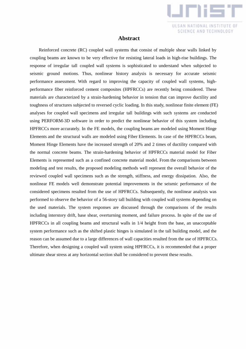
Reinforced concrete (RC) coupled wall systems that consist of multiple shear walls linked by

coupling beams are known to be very effective for resisting lateral loads in high-rise buildings. The

response of irregular tall coupled wall systems is sophisticated to understand when subjected to

seismic ground motions. Thus, nonlinear history analysis is necessary for accurate seismic

performance assessment. With regard to improving the capacity of coupled wall systems, high-

performance fiber reinforced cement composites (HPFRCCs) are recently being considered. These

materials are characterized by a strain-hardening behavior in tension that can improve ductility and

toughness of structures subjected to reversed cyclic loading. In this study, nonlinear finite element (FE)

analyses for coupled wall specimens and irregular tall buildings with such systems are conducted

using PERFORM-3D software in order to predict the nonlinear behavior of this system including

HPFRCCs more accurately. In the FE models, the coupling beams are modeled using Moment Hinge

Elements and the structural walls are modeled using Fiber Elements. In case of the HPFRCCs beam,

Moment Hinge Elements have the increased strength of 20% and 2 times of ductility compared with

the normal concrete beams. The strain-hardening behavior of HPFRCCs material model for Fiber

Elements is represented such as a confined concrete material model. From the comparisons between

modeling and test results, the proposed modeling methods well represent the overall behavior of the

reviewed coupled wall specimens such as the strength, stiffness, and energy dissipation. Also, the

nonlinear FE models well demonstrate potential improvements in the seismic performance of the

considered specimens resulted from the use of HPFRCCs. Subsequently, the nonlinear analysis was

performed to observe the behavior of a 56-story tall building with coupled wall systems depending on

the used materials. The system responses are discussed through the comparisons of the results

including interstory drift, base shear, overturning moment, and failure process. In spite of the use of

HPFRCCs in all coupling beams and structural walls in 1/4 height from the base, an unacceptable

system performance such as the shifted plastic hinges is simulated in the tall building model, and the

reason can be assumed due to a large differences of wall capacities resulted from the use of HPFRCCs.

Therefore, when designing a coupled wall system using HPFRCCs, it is recommended that a proper

ultimate shear stress at any horizontal section shall be considered to prevent these results.

I

Contents

ABSTRACT ..............................................................................................................................................

CONTENTS ............................................................................................................................................. I

LIST OF FIGURES ............................................................................................................................... II

LIST OF TABLES ................................................................................................................................. V

NOMENCLATURE .............................................................................................................................. VI

CHAPTER 1. INTRODUCTION ........................................................................................................... 1

1.1 Background and Motivation.............................................................................................................. 1

1.2 Objectivities ...................................................................................................................................... 2

CHAPTER 2. LITERATURE REVIEW OF COUPLED SHEAR WALLS ........................................... 3

2.1 Behavior of Coupled Shear Walls ..................................................................................................... 3

2.2 Design Criteria of Coupled Shear Walls ........................................................................................... 7

2.3 Previous Experimental Works of Coupled Shear Walls .................................................................... 8

2.4 Modeling Methods of Coupled Wall Systems ................................................................................. 15

CHAPTER 3. DEVELOPMENT OF ANALYSIS METHODS ........................................................... 21

3.1 Force-Deformation Relationship in PERFORM-3D ....................................................................... 21

3.2 Modeling Methods of Coupling Beams .......................................................................................... 21

3.3 Modeling Methods of Shear Walls .................................................................................................. 24

CHAPTER 4. ANALYSIS OF INDIVIDUAL COUPLED SHEAR WALLS ...................................... 28

4.1 Example Structures ......................................................................................................................... 28

4.2 Modeling Processes ........................................................................................................................ 35

4.3 Correlationship of Modeling Results and Experimental Results .................................................... 40

CHAPTER 5. ANALYSIS OF A TALL BUILDING WITH COUPLED SHEAR WALLS ................. 44

5.1 Example Structures ......................................................................................................................... 44

5.2 Modeling Processes ........................................................................................................................ 50

5.3 Analysis Results .............................................................................................................................. 59

CHAPTER 6. CONCLUSIONS ........................................................................................................... 92

REFERENCES .........................................................................................................................................

II

List of Figures

Figure 1 - A Coupled Wall System .......................................................................................................... 3

Figure 2 - Deformation of Coupling Beams under lateral loads ............................................................. 4

Figure 3 - Failure Modes of Coupling Beams ......................................................................................... 4

Figure 4 - Deformed Shape of Walls Subjected to Lateral Loading ....................................................... 5

Figure 5 - Flexural Failure Modes of Structural Walls (Cho, et al. 2007) .............................................. 6

Figure 6 - Shear Failure Modes of the Structural Walls (Cho, et al. 2007) ............................................. 6

Figure 7 - Decomposition of a RC Beam Model (Filippou et al., 1999) .............................................. 15

Figure 8 - Load-Deformation Backbone Curves of Coupling beams by Naish et al. (2010) (dotted line:

1/2-scale) ............................................................................................................................................... 16

Figure 9 – Coupling Beam Models (Naish et al., 2010) ....................................................................... 16

Figure 10 - Beam-Column Element Model for RC Walls (Takayanagi and Schnobrich, 1976) ........... 17

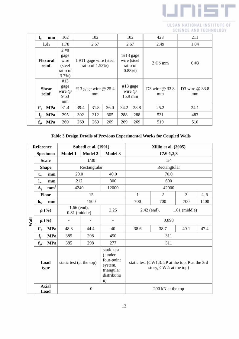
Figure 11 - TVLEM for RC Shear Walls (Kabeyasawa et al., 1983) .................................................... 18

Figure 12 - Force-Deformation Relations of Hysteresis Models for RC Members .............................. 18

Figure 13 - MVLEM for RC Shear Walls (Vulcano et al., 1988) ......................................................... 19

Figure 14 - Modified MVLEM for RC Shear Walls (Colotti, 1993) .................................................... 19

Figure 15 - Fiber Element Model for RC Shear Walls (Petrangeli et al., 1999a) ................................. 20

Figure 16 – Nonlinear Force-Deformation Relationship in PERFORM-3D ........................................ 21

Figure 17 - Coupling Beam Model ....................................................................................................... 22

Figure 18 - Generalized Force-Deformation Relation for Concrete Elements or Components (ASCE

41-06) .................................................................................................................................................... 23

Figure 19 - Force-Deformation Model of Coupling Beams in PERFORM-3D .................................... 24

Figure 20 - Parallel Layers in General Wall Element on PERFORM-3D ............................................. 25

Figure 21 - Shear Wall Fiber Model ..................................................................................................... 26

Figure 22 – Stress-Strain Model of Steel Material ............................................................................... 27

Figure 23 - Stress-Strain Model of Concrete Material .......................................................................... 27

Figure 24 - Example Structures CW-1 Tested by Lequesne (2011) ...................................................... 29

Figure 25 - Example Structures CW-2 Tested by Lequesne (2011) ...................................................... 30

Figure 26 - Coupling Beams in CW-1 & CW-2 (Lequesne, 2011) ....................................................... 31

Figure 27 - Cyclic Loading History (Lequesne, 2011) ......................................................................... 32

Figure 28 - Shear Wall Fiber Model of Individual Coupled Shear Walls ............................................. 36

Figure 29 - Overturning Moment vs. Wall drift for CW-1 .................................................................... 41

Figure 30 - Overturning Moment vs. Wall drift for CW-2 .................................................................... 41

Figure 31 - Coupling Beams of CW-1 .................................................................................................. 42

Figure 32 - Coupling Beams of CW-2 .................................................................................................. 43

III

Figure 33 - Plane View of the Tall Building ......................................................................................... 44

Figure 34 - Cross Sections of CBs in Tall Buildings (unit: mm) .......................................................... 45

Figure 35 - Cross Section of Walls in Tall Buildings ............................................................................ 46

Figure 36 - Mechanism of P- Δ Column ............................................................................................... 56

Figure 37 - Vertical Distributions for Static Push-Over Loads ............................................................. 57

Figure 38 – El Centro Earthquake......................................................................................................... 58

Figure 39 - Mode Shape of TB-1 .......................................................................................................... 59

Figure 40 - Mode Shape of TB-2 .......................................................................................................... 60

Figure 41 - Story Drift under Static Push-Over Loads with Uniform Distribution .............................. 61

Figure 42 - Story Drift under Static Push-Over Loads with Triangular Distribution ........................... 62

Figure 43 - Story Drift under Static Push-Over Loads with C Factor Distribution .............................. 62

Figure 44 - Story Drift under Static Push-Over Loads with Mode Shape Distribution ........................ 64

Figure 45 - Story Drift under Cyclic Push-Over Loads with C-factor Distribution ............................. 65

Figure 46 - Base Shear under Static Push-Over Load without Gravity: Uniform, Triangular and C

Factor Distributions .............................................................................................................................. 67

Figure 47- Base Shear under Static Push-Over Load of without Gravity: Mode Shape Distribution of

TB-1 ...................................................................................................................................................... 67

Figure 48- Base Shear under Static Push-Over Load of without Gravity: Mode Shape Distribution of

TB-2 ...................................................................................................................................................... 68

Figure 49 - Base Shear under Static Push-Over Load with Gravity: Uniform, Triangular and C Factor

Distributions .......................................................................................................................................... 70

Figure 50- Base Shear under Static Push-Over Load with Gravity: Mode Shape Distribution of TB-1

.............................................................................................................................................................. 70

Figure 51- Base Shear under Static Push-Over Load with Gravity: Mode Shape Distribution of TB-2

.............................................................................................................................................................. 71

Figure 52 - Base Shear under Cyclic Push-Over Load ......................................................................... 72

Figure 53 - P-Δ Shear under Static Push-Over Load: Uniform, Triangular and C Factor Distributions

.............................................................................................................................................................. 73

Figure 54 - P-Δ Shear under Static Push-Over Load: Mode Shape Distribution of TB-1 .................... 73

Figure 55 - P-Δ Shear under Static Push-Over Load: Mode Shape Distribution of TB-2 .................... 74

Figure 56 - P-Δ Shear under Cyclic Push-Over Load ........................................................................... 74

Figure 57 - Overturning Moment under Static Push-Over Load: Uniform, Triangular, and C Factor

Distributions .......................................................................................................................................... 75

Figure 58 - Overturning Moment under Static Push-Over Load: Mode Shape Distribution of TB-1 .. 76

Figure 59 - Overturning Moment under Static Push-Over Load: Mode Shape Distribution of TB-2 .. 76

IV

Figure 60 - Overturning Moment under Cyclic Push-Over Load ......................................................... 77

Figure 61 - Torsional Moment under Static Push-Over Load: Uniform, Triangular, and C Factor

Distributions .......................................................................................................................................... 78

Figure 62 - Torsional Moment under Static Push-Over Load: Mode Shape Distribution of TB-1 ....... 78

Figure 63 - Torsional Moment under Static Push-Over Load: Mode Shape Distribution of TB-2 ....... 79

Figure 64 - Torsional Moment under Cyclic Push-Over Load .............................................................. 79

Figure 65 - Location of Strain Gages for Tall Building ........................................................................ 85

Figure 66 - Story Drift under an Earthquake Load at Instant of Maximum Base Shear ....................... 89

Figure 67 - Base Shear under an Earthquake Load ............................................................................... 90

Figure 68 – Story by Story Lateral Force under an Earthquake Load at Instant of Maximum Base

Shear ..................................................................................................................................................... 90

Figure 69 - Overturning Moment under an Earthquake Load ............................................................... 91

Figure 70 - Torsional Moment under an Earthquake Load ................................................................... 91

V

List of Tables

Table 1 Design Details of Previous Experimental Works for Coupled Walls ....................................... 10

Table 2 Design Details of Previous Experimental Works for Coupled Shear Walls ............................. 11

Table 3 Design Details of Previous Experimental Works for Coupled Walls ....................................... 13

Table 4 Modeling Parameters for Coupling Beams in ASCE 41-06 ..................................................... 23

Table 5 Test Variables in Two Specimens ............................................................................................. 32

Table 6 Properties of Normal Concrete ................................................................................................. 33

Table 7 Properties of HPFRCCs ........................................................................................................... 33

Table 8 Results from Tension Tests of Steel Reinforcement ................................................................. 34

Table 9 Modeling Values for Coupling Beams in CW-1 and CW-2 ..................................................... 35

Table 10 Modeling Values for Steel (E = 200GPa) in CW-1 and CW-2 ............................................... 37

Table 11 Modeling Values for Unconfined Concrete in Compression in CW-1 and CW-2 .................. 37

Table 12 Modeling Values for Unconfined Concrete in Tension in CW-1 and CW-2 .......................... 38

Table 13 Modeling Values for Confined Concrete in CW-1 and CW-2 ................................................ 39

Table 14 Reinforcement of Walls in TB-1 and TB-2 (unit: mm) .......................................................... 46

Table 15 Modeling Values for Coupling Beams in TB-1 and TB-2 ...................................................... 50

Table 16 Modeling Values for Steels in TB-1 and TB-2 (E = 200GPa) ................................................ 54

Table 17 Modeling Values for Concrete in TB-1 and TB-2 .................................................................. 54

Table 18 Modeling Values for HPFRCCs in TB-2 ................................................................................ 55

Table 19 Results of Lumped Masses at each floor of Tall Building ..................................................... 55

Table 20 Vertical Distribution Factor Cvw in TB-1 and TB-2 ............................................................... 58

Table 21 Mode Periods of TB-1 ............................................................................................................ 59

Table 22 Mode Periods of TB-2 ............................................................................................................ 60

Table 23 Failure Process of Coupling Beams in TB-1 under Cyclic Push-Over Load ......................... 81

Table 24 Failure Process of Coupling Beams in TB-2 under Cyclic Push-Over Load ......................... 82

Table 25 Failure Process of Walls in TB-1 under Cyclic Push-Over Load ........................................... 85

Table 26 Failure Process of Walls in TB-2 under Cyclic Push-Over Load ........................................... 86

VI

Nomenclature

Ac area of concrete section

Acw area of concrete section of coupling beam resisting shear

Ag gross area

Asd area of each group of the diagonal bars

d distance from extreme compression fiber to centroid of longitudinal tension reinforcements

d’ length of the clear cover

Ec secant modulus of elasticity of concrete

f'c specified compressive strength of concrete

fy specified yield strength of reinforcement

fyt specified yield strength of transverse reinforcement

h height of the beam cross section;

hw height of wall

Icr cracked moment of inertia of the cross section

Ig moment of inertia of gross concrete section

lp plastic hinge length

lw length of wall

Mn nominal flexural strength at section

Mo overturning moment

P axial force

tw thickness of wall

Z slope of the descending branch

α angle with the horizontal axis of the beam;

ε0 strain at the f’c

εc strain in the concrete

ρl ratio of area of distributed longitudinal reinforcement to gross concrete area

ρt ratio of area of distributed transverse reinforcement to gross concrete area

υ poison ratio

1

Chapter 1. Introduction

1.1 Background and Motivation

Tall buildings are expected to contribute greatly to creation of eco-friendly high-tech space by

concentrating land use. Besides, because the tall buildings have the meaning of future-oriented

landmark, the demand for these buildings is gradually increasing. Reinforced concrete (RC) coupled

wall systems are known as the effective structural system resisting lateral loads like earthquakes for

the tall buildings. These structural systems generally consist of two shear walls linked by coupling

beams. Especially, properly designed coupled wall systems contribute greatly to dissipate a substantial

amount of energy with inelastic behavior. For this reason, many extensive researches about the

coupling beams and shear walls are continuously conducted.

Because shear forces are transferred between coupling beams and shear walls, the coupling

beams are required to withstand the high shear forces. Various experiments have been also conducted

to analyze the behavior of coupling beams depending on the aspect ratio and the arrangement of

reinforcement (Paulay 1971, Paulay and Binney 1974, Barney et al. 1980, Tassios et al. 1996, Xiao et

al. 1999, Galano and Vignoli 2000, Kwan and Zhao 2002, Fortney 2005). These studies usually had

the low aspect ratios (the short beam clear span to the beam total depth) which are differ from the

coupling beams in the tall buildings. Recentrly, Naish et al. (2009) experimented the larger aspect-

ratio coupling beams satisfied with the 2008 ACI Code requirement about simplified reinforcement

details.

The continuous researches about development and applicability of construction materials have

been also conducted to get the better durability and structural performance. With regard to the coupled

wall systems, high-performance fiber reinforced cement composites (HPFRCCs) are recently being

assessed as the material with high applicability. In the early years of 1918, the adding of fiber to

improve the week tensile behavior of concrete was beginning of fiber reinforced concrete (FRC).

Based on this, the HPFRCCs were appeared through a various researches and this material has a

multiple crack characteristic and a strain-hardening characteristic (Naaman and Reinhardt, 1996).

Over the past decade, the experimental works about building component including HPFRCCs are

proceeding. The HPFRCCs beam and wall components showed good performance under the reversed

cyclic displacement loading despite the reductions of reinforcement detailing (Canbolat et al. 2005,

Parra-Montesions et al. 2006). Lequesne (2011) showed that the coupled wall systems with HPFRCCs

exhibited a ductile flexural behavior in the walls and the improved damage tolerance in beams. From

the previous studies, the use of HPFRCCs can reduce the requirement of reinforcements and it can

2

simplify the construction work. Because few experimental researches about the coupled wall systems

including HPFRCCs are conducted, the reliable studies about the response of the structure scale

according to the materials are required.

Performance based design is known as the most used method to design of the tall buildings with

coupled wall systems in these days. The important goal of this design is to evaluate the behavior of

structures at different seismic risk levels. The nonlinear analysis must be considered to select the

acceptable behavior of structure for use of the design method. The structure systems basically have

two type of nonlinearity as follows. First one is a material nonlinearity which is usually caused by

inelastic behavior and it is the material property such as yielding, cracking, crushing, fracture, and so

on. The geometric nonlinearity usually caused by change in shape of the structure and it includes P-Δ

effects and true large displacement effects. Although the experimental work for nonlinear analysis is

most accurate way to measure these nonlinear behavior of the structures, it needs to a lot of times and

efforts. Therefore, modeling method for nonlinear analysis is increasingly demanded. The nonlinear

analysis is not for the exact prediction of the structural behavior, but it is to get the useful information

about the structures. For the reliable and economical modeling analysis of the reinforced concrete

structure, proper models of materials or geometry of the structural systems are essential.

1.2 Objectivities

In this study, PERFORM-3D developed by Professor Powell will be used for nonlinear seismic

analysis of a tall building with the coupled wall systems as modeling software.

It was the purpose of this study to:

Review the macroscopic modeling methods for effective nonlinear analysis.

By the application of effective modeling methods to some specimens, assesse the

behavior of the structure system model.

Compare between modeling results and test results, and discuss the reliability of the

modeling and a better method.

Assesse and compare the performance of structures depending on the materials in

coupling beams and the hinge of walls; normal concrete and HPFRCCs.

Apply the reliable modeling method to tall building in structural scale, and investigate the

behavior of an actual core wall system composed of the coupled wall systems as the

different properties of coupling beams and lower sections of the walls through the

nonlinear analysis.

3

Chapter 2. Literature Review of Coupled Shear Walls

2.1 Behavior of Coupled Shear Walls

When the shear walls are connected with the beams, a coupling effect increases the stiffness and

strength of the shear wall system under the lateral loads as shown in Figure 1. This provides

additional resistance to overturning moment Mo, which is calculated by Eq. (1) where M1 is the

moment from the left wall, and M2 is the moment from the right wall. This coupling action by

transferring shear between the walls through the coupling beams is represented with the TL and this

effect reduces the required flexural stiffness and strength of the individual walls. The axial force T can

be calculated with the sum of shear forces at the each coupling beam, and the magnitude of each shear

force is decided by the stiffness and strength of the beam. Therefore, the proper design of coupling

beams is important to the coupled wall systems.

𝐌𝐨(𝐜𝐨𝐮𝐩𝐥𝐞𝐝) = 𝐌𝟏 + 𝐌𝟐 + 𝐓𝐋 Eq. (1)

Figure 1 - A Coupled Wall System

4

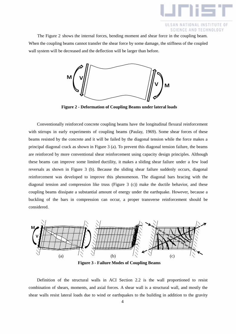
The Figure 2 shows the internal forces, bending moment and shear force in the coupling beam.

When the coupling beams cannot transfer the shear force by some damage, the stiffness of the coupled

wall system will be decreased and the deflection will be larger than before.

Figure 2 - Deformation of Coupling Beams under lateral loads

Conventionally reinforced concrete coupling beams have the longitudinal flexural reinforcement

with stirrups in early experiments of coupling beams (Paulay, 1969). Some shear forces of these

beams resisted by the concrete and it will be failed by the diagonal tension while the force makes a

principal diagonal crack as shown in Figure 3 (a). To prevent this diagonal tension failure, the beams

are reinforced by more conventional shear reinforcement using capacity design principles. Although

these beams can improve some limited ductility, it makes a sliding shear failure under a few load

reversals as shown in Figure 3 (b). Because the sliding shear failure suddenly occurs, diagonal

reinforcement was developed to improve this phenomenon. The diagonal bars bracing with the

diagonal tension and compression like truss (Figure 3 (c)) make the ductile behavior, and these

coupling beams dissipate a substantial amount of energy under the earthquake. However, because a

buckling of the bars in compression can occur, a proper transverse reinforcement should be

considered.

Figure 3 - Failure Modes of Coupling Beams

Definition of the structural walls in ACI Section 2.2 is the wall proportioned to resist

combination of shears, moments, and axial forces. A shear wall is a structural wall, and mostly the

shear walls resist lateral loads due to wind or earthquakes to the building in addition to the gravity

(a) (b) (c)

5

loads from the floors and roofs. These walls have a larger stiffness and a relatively smaller

displacement by shear forces than frame structures. When the height-to-length aspect ratio (hw/𝑙𝑤) of

the walls is less than or equal to 2, the walls are called ‘short or squat walls’. The shear walls have an

aspect ratio of greater than or equal to 3, and these are called slender or flexural walls. The squat walls

respond with a shear behavior in general, and the behavior of slender walls is dominated by flexure.

Figure 4 shows this behavior with exaggerated expressions. The walls in the tall buildings typically

are the slender walls with flexure behavior.

Figure 4 - Deformed Shape of Walls Subjected to Lateral Loading

The failure modes of structural walls can be classified into flexural and shear failures. Figure 5

shows the flexural failure of the walls, and Figure 5 (a) occurs when a vertical reinforcement ratio is

low. The flexural reinforcing bars in tension part are gradually extended and fracture seriately from

the outside at the base of the wall. Before the reinforcements fracture, only one main flexural crack is

formed. Figure 5 (b) shows a shear failure after the occurrence of several flexural cracks, and the

failure mode is due to diagonal tension or diagonal compression caused by shear. Figure 5 (c) is a

general failure mode, and the concrete at the lowest part of wall is finally crushed as yields of flexural

reinforcement are expanded. Figure 6 shows the phenomena of the shear failure mode. Figure 6 (a)

occurs when shear reinforcements are insufficient, and the reinforcing bars crossed the diagonal

cracks resist the diagonal tension. When the diagonal tension failure of Figure 6 (a) is controlled by

the sufficient shear reinforcements and high shear forces can be resisted by these, Figure 6 (b) occurs

if the compressive stress at the compression strut of the wall is over the compressive stress of concrete.

The compression strut will be crushed. Figure 6 (c) represents the sliding shear failure along the

(a) Squat Wall (b) Slender Wall

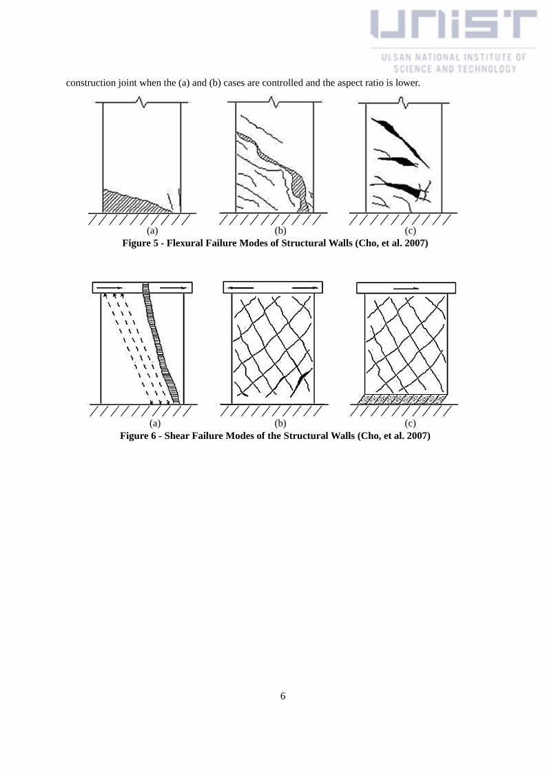
6

construction joint when the (a) and (b) cases are controlled and the aspect ratio is lower.

Figure 5 - Flexural Failure Modes of Structural Walls (Cho, et al. 2007)

Figure 6 - Shear Failure Modes of the Structural Walls (Cho, et al. 2007)

(a) (b) (c)

(a) (b) (c)

7

2.2 Design Criteria of Coupled Shear Walls

In common with the shear walls, the design methods of coupling beams follow the ACI Code in

this study. ACI Code Section 21.9.7 states that coupling beams with aspect ratio (ln/ℎ) ≥ 4 shall

satisfy the requirements of Section 21.5 as the flexural member of a special moment frame with

conventional reinforcement. Coupling beams with ln/ℎ < 2 and with Vu > 0.33√𝑓𝑐′𝐴𝑐𝑤, where Acw

is the coupling beam area, shall be reinforced with two intersecting groups of diagonally placed bars.

The other coupling beams can select the reinforcement type between the diagonally placed bars and

the special moment frame detailing. As a horizontal wall segments, the nominal shear strength of

coupling beam shall be smaller than 0.83𝐴𝑐𝑤√𝑓𝑐′.

Proper design methods are also necessary for shear walls to prevent the brittle fracture behavior

and perform the basic function of resisting lateral loads. The desirable behavior of the walls develops

the flexural hinge at the base of the wall. It means that the flexural reinforcement should be yielded in

the plastic hinge regions to provide ductility of the wall. Generally, the shear walls are designed in

accordance with ACI Code Section 11.9 and Chapter 14. The ultimate shear stresses at any horizontal

section shall be taken smaller than 0.83√𝑓𝑐′. The design methods of special structure walls with high

ductility are given in the ACI Code Section 21.9. A structure which consists of several walls to resist

the factored shear force has the average unit strength limited to 0.66√𝑓𝑐′. For any one of the

individual vertical walls in this structure, the unit shear strength shall not exceed 0.83√𝑓𝑐′. After the

wall cross section is detailed, the parts to be considered for seismic design are boundary elements. For

the walls with a high compression demand at the edge, boundary elements are required and these can

be developed with extra confinement or longitudinal bars at the end of wall or widened end with

confinements.

8

2.3 Previous Experimental Works of Coupled Shear Walls

The response of coupled systems is not simple to be accurately predicted. While the individual

wall or beam components have been actively experimented, relatively few experimental works were

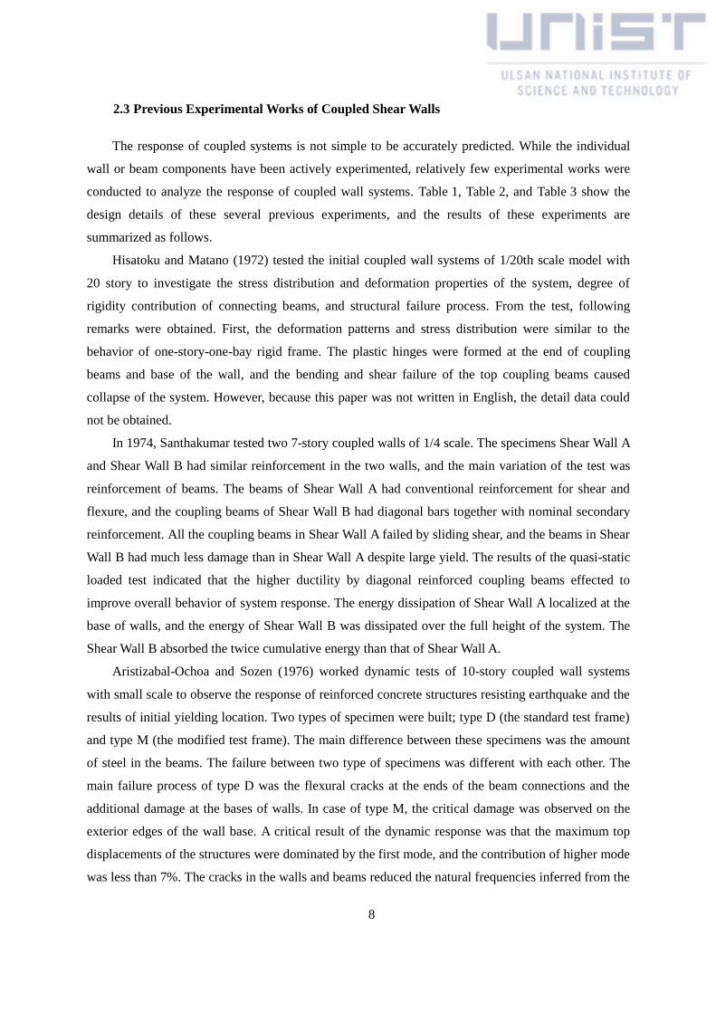
conducted to analyze the response of coupled wall systems. Table 1, Table 2, and Table 3 show the

design details of these several previous experiments, and the results of these experiments are

summarized as follows.

Hisatoku and Matano (1972) tested the initial coupled wall systems of 1/20th scale model with

20 story to investigate the stress distribution and deformation properties of the system, degree of

rigidity contribution of connecting beams, and structural failure process. From the test, following

remarks were obtained. First, the deformation patterns and stress distribution were similar to the

behavior of one-story-one-bay rigid frame. The plastic hinges were formed at the end of coupling

beams and base of the wall, and the bending and shear failure of the top coupling beams caused

collapse of the system. However, because this paper was not written in English, the detail data could

not be obtained.

In 1974, Santhakumar tested two 7-story coupled walls of 1/4 scale. The specimens Shear Wall A

and Shear Wall B had similar reinforcement in the two walls, and the main variation of the test was

reinforcement of beams. The beams of Shear Wall A had conventional reinforcement for shear and

flexure, and the coupling beams of Shear Wall B had diagonal bars together with nominal secondary

reinforcement. All the coupling beams in Shear Wall A failed by sliding shear, and the beams in Shear

Wall B had much less damage than in Shear Wall A despite large yield. The results of the quasi-static

loaded test indicated that the higher ductility by diagonal reinforced coupling beams effected to

improve overall behavior of system response. The energy dissipation of Shear Wall A localized at the

base of walls, and the energy of Shear Wall B was dissipated over the full height of the system. The

Shear Wall B absorbed the twice cumulative energy than that of Shear Wall A.

Aristizabal-Ochoa and Sozen (1976) worked dynamic tests of 10-story coupled wall systems

with small scale to observe the response of reinforced concrete structures resisting earthquake and the

results of initial yielding location. Two types of specimen were built; type D (the standard test frame)

and type M (the modified test frame). The main difference between these specimens was the amount

of steel in the beams. The failure between two type of specimens was different with each other. The

main failure process of type D was the flexural cracks at the ends of the beam connections and the

additional damage at the bases of walls. In case of type M, the critical damage was observed on the

exterior edges of the wall base. A critical result of the dynamic response was that the maximum top

displacements of the structures were dominated by the first mode, and the contribution of higher mode

was less than 7%. The cracks in the walls and beams reduced the natural frequencies inferred from the

9

displacement and acceleration waveforms. A triangular distribution of lateral load was recommended

to the most proper vertical distribution, because the centroid of lateral action was located at 0.7 times

of the wall height.

Other tests of small-scale coupled systems with 6 stories were conducted by Lybas and Sozen

(1977). The five reinforced concrete coupled wall systems were subjected to earthquake base motions,

and an additional specimen was subjected to static lateral loading. The principal variable in the

specimens was the strength and stiffness of the connecting beams. The specimens were grouped into

three classes (Type A, Type B, and Type C) according to their beam cross-section. As results from the

experiment, type A under the dynamic loading was failed by the development of the maximum tensile

capacity at the wall bases without any yields of beams. The failure mechanisms of Type B and C

under the dynamic loads were similar to each other, and these specimens had a flexural yielding at the

ends of the beams first and at the bases of walls subsequently. The tests showed that the natural

frequency of the specimens decreased under the increased and continuous base motion. As the

strength and stiffness of the coupling beams were decreased, the relative contribution to base shears

and moments of higher modes increased. As the results of the static hysteretic analysis, the beams

significantly contributed to the overall hysteresis of the structure.

Shiu et al. (1981) conducted the two coupled wall tests with 6 story of 1/3 scale to determine

effects of coupling beam on the coupled wall. A system with weak coupling beams (CS-1) and a

system with strong repaired beams (RCS-1) were used for this test. The coupling beams in CS-1 was

yielded relatively early in the test, and the beams could not dissipate a sufficient energy. This resulted

in the separate behavior of the walls. The RCS-1 resulted in large axial stresses which caused web

crushing in the base of the walls, because the beams had relatively too strong than the walls. This was

noted that beams require a sufficient deformation capacity to remain the coupling action. At the same

time, the walls should maintain the axial load when the coupling beams dissipate the sufficient energy.

Three coupled structural walls with approximately l/30th scale of a 15-story building were tested

to investigate failure modes (Subedi, 1991). The different dimensions of the specimens were chosen

for the different failure mode; flexural, shear, and composite. Two types of loadings were applied.

Model 1 and 2 were tested under a point load at the top and Model 3 was tested under a four-point

system for triangular distribution over the height. The three specimens represented the intended modes

of failure. Model 1 was failed with flexure behavior at nearly all coupling beams and crushing of

compression wall. The walls of Model 2 were failed compositely with minor damage in coupling

beams. The failure mechanism of Model 3 consisted of shear failure in beams followed by crushing of

compression wall. Although the size of three specimens was a small range of practical structure, it

was clear that the coupling beam greatly affected on the behavior of the coupled wall systems.

Xillin et al. (2005) tested three coupled walls of 1/4 scale with 5 stories, named CW-1, CW-2,

10

and CW-3. The height of coupling beams was the variables of this test, and it made different coupling

ratio between the walls. The horizontal loading was applied to the specimens. CW-1 and CW-3 were

loaded at two points to represent the inverted triangular load, and CW-2 was loaded at one point of the

top. The results of cracking procedure were very similar to each other, and the failures of all

specimens occurred at the bottom of the walls. However, CW-1 was dominated by flexure failure,

CW-3 was dominated by shear failure, and the both failure modes were represented in CW-2.

Although the more damages of coupling beams were expected to prevent the failure of walls

according to the design code (JGJ 101-96 in China), the different results were occurred at this

experiment. There were no details about these results in this paper because the purpose of the study

was the verification of a nonlinear model.

The main purpose of the previous tests was to understand the behavior of coupled wall structures

depending on the design of coupling beams. As the writer’s knowledge, there is one of experimental

works for coupled wall systems using HPFRCCs. This was conducted by Lequesne in 2011, and the

details will be considered in Chapter 4 to compare the results by nonlinear analysis.

Table 1 Design Details of Previous Experimental Works for Coupled Walls

Reference Santhakumar (1974) Aristizabal-Ochoa et al. (1976)

Wall

Specimen Shear Wall A & Shear Wall B type-D type-M

Scale 1/4 1/12

Shape Rectangtular Rectangtular

tw mm 102 25.4

lw mm 610 178

Ag mm2 61900 4520

Floor 1~3F 4F 5F 6, 7F 1~3F 4, 5F 6~10F 1~3F 4, 5F 6~10F

hw mm 3960 762 762 1520 686 457 1240 686 457 1240

ρl (%)

3.49

(end),

0.700

(midd

le)

2.79

(end),

0.700

(middl

e)

2.09

(end),

0.700

(middl

e)

1.39

(end),

0.700

(midd

le)

3.30 (end),

0.61

(middle)

1.65

(end),

0.600

(middle

)

3.30 (end)

ρt (%) 0.88 0.67 0.67 0.44

0.310

(whol

e)

1.33

(confi

nment

)

0.31

0.410

(whol

e)

1.33

(confi

nment

)

0.41

f'c MPa 36.4 (A), 38.2 (B) 32.5 32.8

fy MPa 305 496 (#8 wire), 731 (#16 wire)

fyt MPa 352 731

11

Load

type

static test (under three-point

system, triangular distribution) dynamic test (with base motion)

Axial

load

25 kips (111kN) using two

prestressed cables at the centroid

of each wall

1000 lb (4.45 kN) at

each of the ten stories

1000 lb (4.45 kN) at

each of the ten stories

P/Acfc'

0.025

7 (A),

0.024

5 (B)

0.0256

(A),

0.0244

(B)

0.0254

(A),

0.0242

(B)

0.025

2 (A),

0.024

(B)

0.155 (at the

base)

0.0767

(at the

6th

story)

0.154 (at the base)

P/Agfc'

0.024

7 (A),

0.023

5 (B)

0.0247

(A),

0.0235

(B)

0.0247

(A),

0.0235

(B)

0.024

7 (A),

0.023

5 (B)

0.152 (at the

base)

0.0758

(at the

6th

story)

0.150 (at the base)

Bea

m

Specimen Shear Wall A Shear Wall B type-D type-M

Reinf.

type

conventional diagonal conventional

doubly reinforced doubly reinforced

t mm 76.2 25.4 25.4

h mm 305 38.1 38.1

Ag mm2 23200 968 968

ln mm 381 102 102

ln/h 1.25 2.67 2.67

Flexural

reinf. 2 #3 bars

2 #3 bars & 2

Φ6.35 mm bars 1 #8 gage wire 4 #8 gage wire

Shear

reinf.

Φ6.35 mm @

50.8 mm

Φ4.76 mm @

114 mm

10 #16 gage wire @

11.43 mm

20 #16 gage wire @

5.334 mm

f'c MPa 36.4 38.2 32.5 32.8

fy MPa 315 315 & 346 496 496

fyt MPa 346 230 731 731

Table 2 Design Details of Previous Experimental Works for Coupled Shear Walls

Reference Lybas et al. (1977) Shiu et al. (1981)

Wa

ll Specimen D1 D2 D3 S1 D4 D5 CS-1, RCS-1

Scale 1/11 1/3

Shape Rectangtular Rectangtular

12

tw mm 25.4 102

lw mm 178 1910

Ag mm2 4520 194000

Floor 6 1 2 3 4 5 6

hw mm 1520 5490

ρl (%) 0.980 6.15 (end), 0.370 (middle)

ρt (%) 1.11

0.550

(whole),

0.410

(confinme

nt)

0.550 (whole), 0.140

(confinment)

f'c MPa 31.4 39.4 31.8 36.0 34.2 28.8 30.5 23.4 25.

8 25.0

21.

0

25.

9

fy MPa 291 302 312 305 307 308 434 (#4), 531(Φ6)

fyt MPa 291 302 312 307 308 305 531 (Φ6), 510 (D3)

Load

type

dynamic test (with

base motion)

static

test

(5P

at 6th

story,

3P at

4th

story,

and P

at

2nd

story)

dynamic

test (with

base

motion)

static test (at the top)

Axial

load

2000 lb (8.90 kN) at each of 2nd, 4th, and 6th

story 0

P/Acfc' 0.095

1

0.075

8

0.093

9

0.082

9

0.08

73

0.10

4 0

P/Agfc' 0.094

2

0.075

1

0.093

0

0.082

1

0.08

64

0.10

3 0

Bea

m

Specimen Type A Type B Type C CS-1 RCS-1

Reinf.

type

Conventional conventional

doubly reinforced doubly reinforced

t mm 25.4 25.4 25.4 102 254

h mm 57.2 38.1 38.1 170 203

Ag mm2 1450 968 968 17300 51600

13

ln mm 102 102 102 423 211

ln/h 1.78 2.67 2.67 2.49 1.04

Flexural

reinf.

2 #8

gage

wire

(steel

ratio of

3.7%)

1 #11 gage wire (steel

ratio of 1.52%)

1#13 gage

wire (steel

ratio of

0.88%)

2 Φ6 mm 6 #3

Shear

reinf.

#13

gage

wire @

9.53

mm

#13 gage wire @ 25.4

mm

#13 gage

wire @

15.9 mm

D3 wire @ 33.8

mm

D3 wire @ 33.8

mm

f'c MPa 31.4 39.4 31.8 36.0 34.2 28.8 25.2 24.1

fy MPa 295 302 312 305 288 288 531 483

fyt MPa 269 269 269 269 269 269 510 510

Table 3 Design Details of Previous Experimental Works for Coupled Walls

Reference Subedi et al. (1991) Xillin et al. (2005)

Wall

Specimen Model 1 Model 2 Model 3 CW-1,2,3

Scale 1/30 1/4

Shape Rectangtular Rectangtular

tw mm 20.0 40.0 70.0

lw mm 212 300 600

Ag mm2 4240 12000 42000

Floor 15 1 2 3 4, 5

hw mm 1500 700 700 700 1400

ρl (%) 1.66 (end),

0.81 (middle) 3.25 2.42 (end), 1.01 (middle)

ρt (%) - - - 0.898

f'c MPa 48.3 44.4 40 38.6 38.7 40.1 47.4

fy MPa 385 298 450 311

fyt MPa 385 298 277 311

Load

type

static test (at the top)

static test

( under

four-point

system,

triangular

distributio

n)

static test (CW1,3: 2P at the top, P at the 3rd

story, CW2: at the top)

Axial

Load 0 200 kN at the top

14

P/Acfc' 0 0.0625 (at

the base)

0.0624 (at

the base)

0.0602

(at the

base)

0.050

9 (at

the

base)

P/Agfc' 0 0.0617 (at

the base)

0.0615 (at

the base)

0.0594

(at the

base)

0.050

2 (at

the

base)

Bea

m

Specimen Model 1 Model 2 Model 3 CW-1 CW-2 CW-3

Reinf.

type

conventional conventional

doubly reinforced doubly reinforced

t mm 20.0 20.0 40.0 70.0 70.0 70.0

h mm 20.0 50.0 30.0 200 250 300

Ag mm2 400 1000 1200 14000 17500 21000

ln mm 75.0 75.0 90.0 400 400 400

ln/h 3.75 1.50 3.00 2.00 1.60 1.33

Flexural

reinf. 2 SWG14

2

SWG10

2

Φ4.75mm

4Φ8, (2Φ8

at middle)

4Φ8, (2Φ8

at middle)

4Φ8,

(2Φ8 at

middle)

Shear

reinf.

7 SWG19

@

12.5mm

4

SWG19

@ 25mm

7 Φ2.0mm

@ 15mm

Φ4 @

50mm

Φ4 @

50mm

Φ4 @

50mm

f'c MPa 48.3 44.4 40.0 38.6 38.6 38.6

fy MPa 385 298 450 278 278 278

fyt MPa 385 298 277 797 797 797

15

2.4 Modeling Methods of Coupled Wall Systems

2.4.1 Coupling Beam Models

The response of coupled wall systems is not simple to experiment the real scale structure. In

order to predict the nonlinear behavior of these systems more accurately, extensive analytical

researches are conducted. The modeling methods can be classified into microscopic models and

macroscopic models. This study will mainly deal with the macroscopic modeling methods using

simplified member of the structure to apply it for the analysis of a tall building.

The linear element models were studied by Aristizabal-Ochoa (1983) and this model was

compared with the experimental results. The massless line elements were used instead of the members

of structure at the centroid, and the joints had finite dimensions with rigid links at the each end of the

beams. This model analyzed the flexural deformations and shear deformations. The rotational inertia

was not considered, only the inertia forces paralleled to the plane were considered.

Nayar and Coull (1976) studied the linear element with hinged plastic ends to present the elastic-

plastic analysis. The stiffness of beams is reduced due to the cracking and this paper represented the

effect by using the hinges. The hinges were formed in an intersection between coupling beam and

walls after the beam reached the ultimate moment or shear capacity. The members had a bilinear

moment-rotation relationship.

Filippou’s model (1999) discussed subelement with varied stiffness in different regions to

represent the effect of reinforcement slip in critical region. The subelements described the force–

displacement relationships. Three subelements were used in the paper such as elastic subelement,

spread plastic subelement, and interface bond-slip subelement as shown in Figure 7. The elastic

subelement modeled the linear elastic behavior of the element until yielding behavior, the spread

plastic subelement modeled the post-yield behavior of the member, and the interface bond-slip

subelement modeled the fixed-end rotations at the interface by the bond deterioration and

reinforcement slip. The joint panel zone was assumed to be rigid.

Figure 7 - Decomposition of a RC Beam Model (Filippou et al., 1999)

16

Naish et al. (2010) studied the modeling of reinforced concrete coupling beams to assess the

current modeling approaches. Especially, this paper focused on the modeling parameters about

effective elastic stiffness, deformation capacity, and residual strength. The effective elastic bending

and shear stiffness values are required for elastic analysis. The effective bending stiffness at yield has

to consider the slip/extension impact of the reinforcement. ASCE 41-06 (2007) defined this; 0.12EcIg

for the test beams. The load-deformation backbone relations for full scale beams were shown in

Figure 8 describing the results of tests and ASCE 41-06 model. The total chord rotations of test beams

at yield, strength degradation, and residual strength were 0.7%, 6.0%, and 9.0% respectively. The

residual strength for tests was 0.3Vn up to 10 ~ 12% rotation and it was 0.8 Vn at plastic rotation of 5%

for ASCE 41-06. This study included the application of the models to computer modeling (CSI,

PERFORM3D). There were two types of model as shown in Figure 9. First models (Figure 9 (a)) had

the moment hinge using a rotational spring at each end of beam to describe the nonlinear

deformations. Figure 9 (b) model had the shear-displacement spring at the middle of the beam to

model the nonlinear deformations. Both models incorporated the elastic slip/extension springs at each

end and elastic beam cross-section.

Figure 8 - Load-Deformation Backbone Curves of Coupling beams by Naish et al. (2010)

(dotted line: 1/2-scale)

Figure 9 - Coupling Beam Models (Naish et al., 2010)

(a) Moment Hinge Model (b) Shear Hinge Model

17

2.4.2 Shear Wall Models

Various models for walls have been proposed to improve some drawbacks by limited conditions.

In the early stage of modeling, an important object of modeling methods was to develop more simple

and accurate model, and each element of the coupled systems was replaced with flexural elements.

The general modeling approach for wall hysteretic behavior was the Beam-Column Element Model

(Takayanagi and Schnobrich, 1976) as shown in Figure 10. The main components of this model are an

elastic flexural element, two nonlinear axial springs, and two nonlinear rotational springs. The elastic

flexural element is account for flexural behavior of the wall, nonlinear axial springs represent the

inelastic behavior at the end of the wall, and nonlinear rotational springs at each end describe inelastic

behavior related with plastic hinge and fixed-end rotation of wall element. Although the modeling

method is simple and easy, it cannot describe the important features of wall behavior like the variation

of neutral axis of the wall cross section, rocking of the wall, and interaction with the frame members

around the wall.

Figure 10 - Beam-Column Element Model for RC Walls (Takayanagi and Schnobrich, 1976)

The Three-Vertical-Line-Element Model (TVLEM) was proposed by Kabeyasawa et al. (1983) as

shown in Figure 11 to explain the variation of neutral axis and interaction with the frame members

connected with the wall. The vertical springs and rotational spring account for the flexural behavior of

the wall, and the horizontal spring accounts for the shear behavior of the wall. The axial force-

deformation relation of the three vertical line elements was modeled with an axial-stiffness hysteresis

model (ASHM, Figure 12 (a)), and the force-deformation relation of both the rotational and horizontal

springs at the wall centerline was modeled with an origin-oriented hysteresis model (OOHM, Figure

12 (b)). This modeling method assumes that the shear stiffness degradation is independent of the axial

force and bending moment. Therefore, the TVLEM cannot precisely describe the actual structure

behavior when the wall systems are governed by shear.

18

Figure 11 - TVLEM for RC Shear Walls (Kabeyasawa et al., 1983)

Figure 12 - Force-Deformation Relations of Hysteresis Models for RC Members

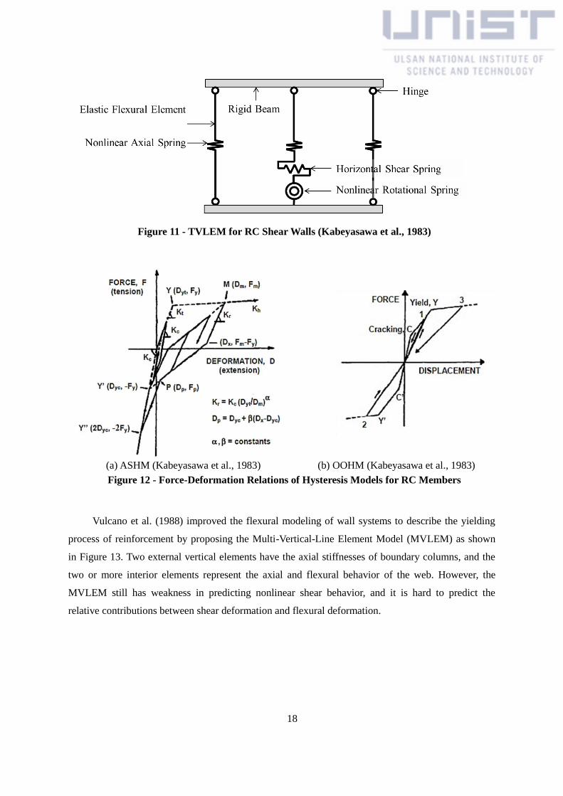
Vulcano et al. (1988) improved the flexural modeling of wall systems to describe the yielding

process of reinforcement by proposing the Multi-Vertical-Line Element Model (MVLEM) as shown

in Figure 13. Two external vertical elements have the axial stiffnesses of boundary columns, and the

two or more interior elements represent the axial and flexural behavior of the web. However, the

MVLEM still has weakness in predicting nonlinear shear behavior, and it is hard to predict the

relative contributions between shear deformation and flexural deformation.

(a) ASHM (Kabeyasawa et al., 1983) (b) OOHM (Kabeyasawa et al., 1983)

19

Figure 13 - MVLEM for RC Shear Walls (Vulcano et al., 1988)

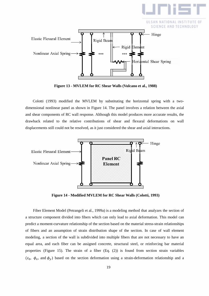
Colotti (1993) modified the MVLEM by substituting the horizontal spring with a two-

dimensional nonlinear panel as shown in Figure 14. The panel involves a relation between the axial

and shear components of RC wall response. Although this model produces more accurate results, the

drawback related to the relative contributions of shear and flexural deformations on wall

displacements still could not be resolved, as it just considered the shear and axial interactions.

Figure 14 - Modified MVLEM for RC Shear Walls (Colotti, 1993)

Fiber Element Model (Petrangeli et al., 1999a) is a modeling method that analyzes the section of

a structure component divided into fibers which can only lead to axial deformation. This model can

predict a moment-curvature relationship of the section based on the material stress-strain relationships

of fibers and an assumption of strain distribution shape of the section. In case of wall element

modeling, a section of the wall is subdivided into multiple fibers that are not necessary to have an

equal area, and each fiber can be assigned concrete, structural steel, or reinforcing bar material

properties (Figure 15). The strain of a fiber (Eq. (2)) is found from section strain variables

(𝜀0, 𝜙𝑥 , and 𝜙𝑦 ) based on the section deformation using a strain-deformation relationship and a

20

shape function. The stress of a fiber (Eq. (3)) is calculated from the fiber strain using relevant

constitutive models, and the stresses are integrated over the cross-sectional area to obtain stress

resultants such as force or moment.

𝜺𝒊 = 𝜺𝟎 + 𝒚𝒊𝝓𝒙 + 𝒙𝒊𝝓𝒚 Eq. (2)

𝝈𝒊 = 𝑬𝒊𝜺𝟎 + 𝑬𝒊𝒚𝒊𝝓𝒙 + 𝑬𝒊𝒙𝒊𝝓𝒚 Eq. (3)

Once, the section forces that are associated with the section deformation are known, the

corresponding wall forces can be calculated using the virtual work principle. However, since this

model is also used restrictively in the shear deformation analysis, the Fiber-Spring Element Model

(FSEM) was proposed by combining a shear spring with a fiber element to reflect the shear

deformation (Lee et al., 2011).

Figure 15 - Fiber Element Model for RC Shear Walls (Petrangeli et al., 1999a)

Previously proposed nonlinear modeling methods for coupled wall systems describe the actual

behavior well, in the case of structures governed by flexure. The main flaw of macroscopic modeling

methods is that the general shear force/shear deformation relation does not coincide with the shear

behavior at the plastic hinge region after flexural yielding. In other words, although the shear

deformation is affected by the flexural cracks that occur before shear cracking, most models could not

reflect this. If the shear deformation is predicted as a function of the wall aspect ratio, the FSEM can

obtain more accurate results than the Fiber Element Model. However, since the experimental results

or precise finite element analysis are required for the parameter setting of the shear springs, it takes

substantial efforts to implement the FSEM. When the RC shear wall is expected to show the shear

dominant behavior, a more simple and reasonable analytical model is required to predict the

interaction between the flexural and shear deformations.

21

Chapter 3. Development of Analysis Methods

3.1 Force-Deformation Relationship in PERFORM-3D

Figure 16 shows the force-deformation model for most of the inelastic components, and it can

describe the hysteric property in detail. The point Y is about yielding stress and strain. The point U

and L as a peak stress means the ultimate stress and strain of the materials and can express a ductile

limit. The point R can consider a remaining stress of material, and point X is about maximum strain of

material. This model is trilinear relationship with strength loss, and the bilinear or no strength loos

model also can be constructed according to user selection.

Figure 16 – Nonlinear Force-Deformation Relationship in PERFORM-3D

3.2 Modeling Methods of Coupling Beams

The coupling beams have significant inelastic deformation capacities, and the beams must

maintain high stiffness and strength for meaningful degree of coupling. The conventional

reinforcement is commonly used in the coupling beams, and it consists of the longitudinal

reinforcement for flexural and transverse reinforcement for shear. In case of the coupling beams

using diagonal reinforcement, the flexure and shear is resisted by this diagonal reinforcement which

have better retention of strength, stiffness, and energy dissipation than the conventional

reinforcement.

As the nonlinear modeling is required for the tall buildings design under the seismic loads,

Naish, at al. (2010) model which is the relatively simple and accurate application method will be

22

used in the coupling beam modeling to estimate and develop the modeling methods using computer

program. The ASCE 41-06 modeling parameters for coupling beams will be used in this paper.

The coupling beams used in this study are expected to develop flexural yielding at their both

ends. Accordingly, the model of the coupling beam consists of a ‘Moment Hinge of Rotation Type’ on

each end and an ‘Elastic Beam Section’ arranged in series as shown in Figure 17. The rigid-plastic

moment hinges in PERFORM-3D indicate the inelastic bending behavior. The hinges can rotate when

the moment of beams reaches the yield moment. Before the yielding of the beam, the stiffness of

beam is expressed by the elastic segment and the deformation of this element is in the elastic part.

And then, after the yield moment is reached, the rigid-plastic moment hinges represent the plastic

deformation with hinge rotation. Naish et al. (2010) recommended the conservative effective elastic

stiffness with 0.20EcIg in the cross section instead of slip/extension hinge. In other words, because this

parameter includes the effect of slip/extension deformations on the overall load-deformation behavior,

the slip/extension hinge could be excluded. This makes the coupling beam models more efficient in a

tall building model that needs many components.

Figure 17 - Coupling Beam Model

The plastic hinge model assumed that all inelastic deformation is concentrated in zero length

plastic hinges. ASCE/SEI 41-06 suggested the use of tabulated modeling parameter (Table 4) to

approach backbone curves (Figure 18) for the nonlinear behavior of the coupling beam. The

generalized force is yield moment and the generalized deformation for the beams is the rotation in the

flexural plastic hinge zone. In Figure 18, A is an unloaded component, B is an effective yield point,

significant strength degradation begins at point C, and the degraded strength up to D is maintained up

to E. The parameters ‘a’ and ‘b’ are the portions of deformation after yielding, and the parameter ‘c’ is

the reduced resistance. The parameters ‘d’ and ‘e’ are the total deformation from origin. Figure 19

shows the force-deformation model to represent this code in PERFORM-3D. The U point in this

figure corresponds to the B point in the code figure. The other points C, D, and E were matched with

L, R, and X respectively.

23

Figure 18 - Generalized Force-Deformation Relation for Concrete Elements or Components

(ASCE 41-06)

Table 4 Modeling Parameters for Coupling Beams in ASCE 41-06

Reinforcement

configuration

𝑽

𝒃𝒘𝒉√𝒇𝒄′

Controlled by flexure Controlled by shear

a b c d e c

With conforming

transverse reinforcement

≤ 0.250 0.0250 0.0500 0.750 0.0200 0.0300 0.600

≥ 0.500 0.0200 0.0400 0.500 0.0160 0.0240 0.300

With nonconforming

transverse reinforcement

≤ 0.250 0.0200 0.0350 0.500 0.0120 0.0250 0.400

≥ 0.500 0.0100 0.0250 0.250 0.00800 0.0140 0.200

Diagonal reinforcement n.a. 0.0300 0.0500 0.800 - - -

24

Figure 19 - Force-Deformation Model of Coupling Beams in PERFORM-3D

The confinement effect by using HPFRCCs in beams can help to prevent buckling, and

HPFRCCs can improve toughness and increase the energy dissipation capacity of the coupling beams.

HPFRCCs increase the maximum shear stress of coupling beams from ACI Code with approximately

40% (Canbolat et al., 2005). The HPFRCCs coupling beams may have increased the flexural strength

by the strain hardening of HPFRCCs and can also improve the ductility through distributing damage

over multiple cracks. These will be modeled with 1.2 times of flexural strength and 2 times of

ductility in this study.

3.3 Modeling Methods of Shear Walls

In the PERFORM-3D software, two kinds of wall elements are usually considered to predict the

wall behavior. A ‘Shear Wall Element’ model is mainly for the relatively slender shear wall structures,

and a ‘General Wall Element’ model is to analyze the complex reinforced concrete walls with

irregular openings (Computer and Structures Inc., 2006). A General Wall Element consists of all of the

parallel five layers as shown in Figure 20 to describe the axial-bending, shear and diagonal

compression behavior. However, the Shear Wall Element consists of the (a) and (c) layers in Figure 20

to consider the vertical axial-bending and shear behavior.

Because the flexural failures of the specimens were expected due to the large slenderness ratio of

the example structures used in this study, the Shear Wall Element can be enough to describe this

structural behavior rather than the General Wall Element. An elastic shear deformation is considered

using a shear material model. The horizontal stiffness and the out-of-plane stiffness are assumed to be

elastic in the Shear Wall Element.

25

Figure 20 - Parallel Layers in General Wall Element on PERFORM-3D

The shear wall element bases on the ‘Inelastic Fiber Element’ for the vertical axial-bending

behavior. The wall element is comprised of the fiber element which performs only axial deformation.

This fiber model can consider the variation of neutral axis by the axial force. As the fiber model bases

on a material stress-strain relation of each fiber and an assumption of the deformed distribution shape

of the cross section, a relatively exact moment-curvature relation of the cross section can be predicted.

Therefore, when the wall element was properly constructed with the material model in fiber, the

nonlinear behavior such as the confinement effect by transverse steels, the concrete crushing, the

tensile cracks of the concrete, the tensile yielding of the steel and the fractures can be precisely

described. In other words, it can describe some complex behavior occurred at the reinforcement and

concrete more exactly.

After dividing the walls with this shear wall element, the each elements of wall was divided

again with fiber unit about the horizontal cross-section of shear wall as shown in Figure 21. The shear

wall model consists of a combination of multiple discretized ‘concrete fiber elements’ and ‘steel fiber

elements’, which are embedded in a series of shear wall elements.

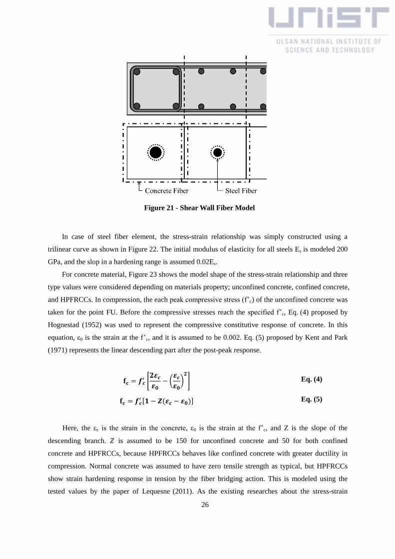
26

Figure 21 - Shear Wall Fiber Model

In case of steel fiber element, the stress-strain relationship was simply constructed using a

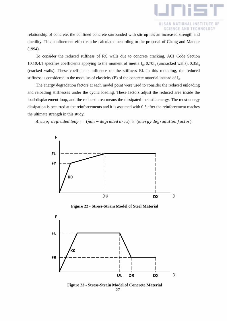
trilinear curve as shown in Figure 22. The initial modulus of elasticity for all steels Es is modeled 200

GPa, and the slop in a hardening range is assumed 0.02Es.

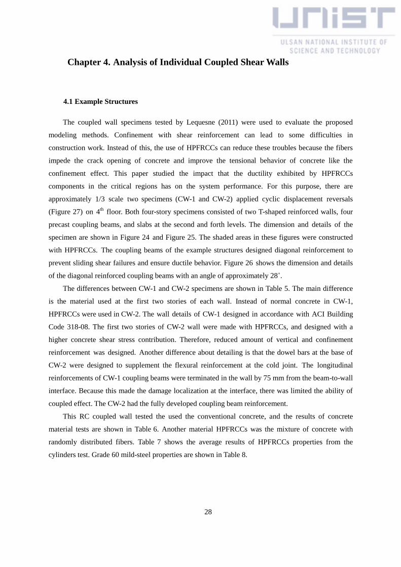
For concrete material, Figure 23 shows the model shape of the stress-strain relationship and three

type values were considered depending on materials property; unconfined concrete, confined concrete,

and HPFRCCs. In compression, the each peak compressive stress (f’c) of the unconfined concrete was

taken for the point FU. Before the compressive stresses reach the specified f’c, Eq. (4) proposed by

Hognestad (1952) was used to represent the compressive constitutive response of concrete. In this

equation, ε0 is the strain at the f’c, and it is assumed to be 0.002. Eq. (5) proposed by Kent and Park

(1971) represents the linear descending part after the post-peak response.

𝐟𝐜 = 𝒇𝒄′ [

𝟐𝜺𝒄

𝜺𝟎− (

𝜺𝒄

𝜺𝟎)

𝟐

] Eq. (4)

𝐟𝐜 = 𝒇𝒄′ [𝟏 − 𝒁(𝜺𝒄 − 𝜺𝟎)] Eq. (5)

Here, the εc is the strain in the concrete, ε0 is the strain at the f’c, and Z is the slope of the

descending branch. 𝑍 is assumed to be 150 for unconfined concrete and 50 for both confined

concrete and HPFRCCs, because HPFRCCs behaves like confined concrete with greater ductility in

compression. Normal concrete was assumed to have zero tensile strength as typical, but HPFRCCs

show strain hardening response in tension by the fiber bridging action. This is modeled using the

tested values by the paper of Lequesne (2011). As the existing researches about the stress-strain

27

relationship of concrete, the confined concrete surrounded with stirrup has an increased strength and

ductility. This confinement effect can be calculated according to the proposal of Chang and Mander

(1994).

To consider the reduced stiffness of RC walls due to concrete cracking, ACI Code Section

10.10.4.1 specifies coefficients applying to the moment of inertia Ig; 0.70Ig (uncracked walls), 0.35Ig

(cracked walls). These coefficients influence on the stiffness EI. In this modeling, the reduced

stiffness is considered in the modulus of elasticity (E) of the concrete material instead of Ig.

The energy degradation factors at each model point were used to consider the reduced unloading

and reloading stiffnesses under the cyclic loading. These factors adjust the reduced area inside the

load-displacement loop, and the reduced area means the dissipated inelastic energy. The most energy

dissipation is occurred at the reinforcements and it is assumed with 0.5 after the reinforcement reaches

the ultimate strength in this study.

𝐴𝑟𝑒𝑎 𝑜𝑓 𝑑𝑒𝑔𝑟𝑎𝑑𝑒𝑑 𝑙𝑜𝑜𝑝 = (𝑛𝑜𝑛 − 𝑑𝑒𝑔𝑟𝑎𝑑𝑒𝑑 𝑎𝑟𝑒𝑎) × (𝑒𝑛𝑒𝑟𝑔𝑦 𝑑𝑒𝑔𝑟𝑎𝑑𝑎𝑡𝑖𝑜𝑛 𝑓𝑎𝑐𝑡𝑜𝑟)

Figure 22 - Stress-Strain Model of Steel Material

Figure 23 - Stress-Strain Model of Concrete Material

28

Chapter 4. Analysis of Individual Coupled Shear Walls

4.1 Example Structures

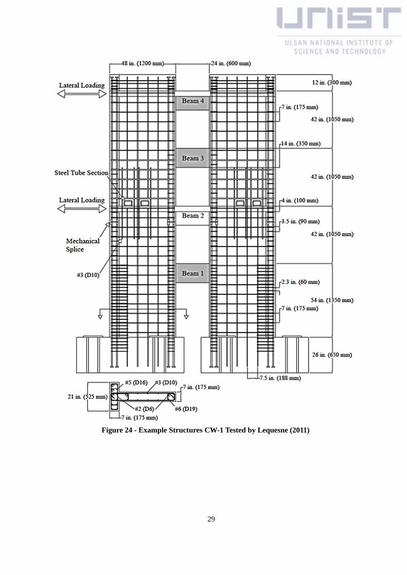
The coupled wall specimens tested by Lequesne (2011) were used to evaluate the proposed

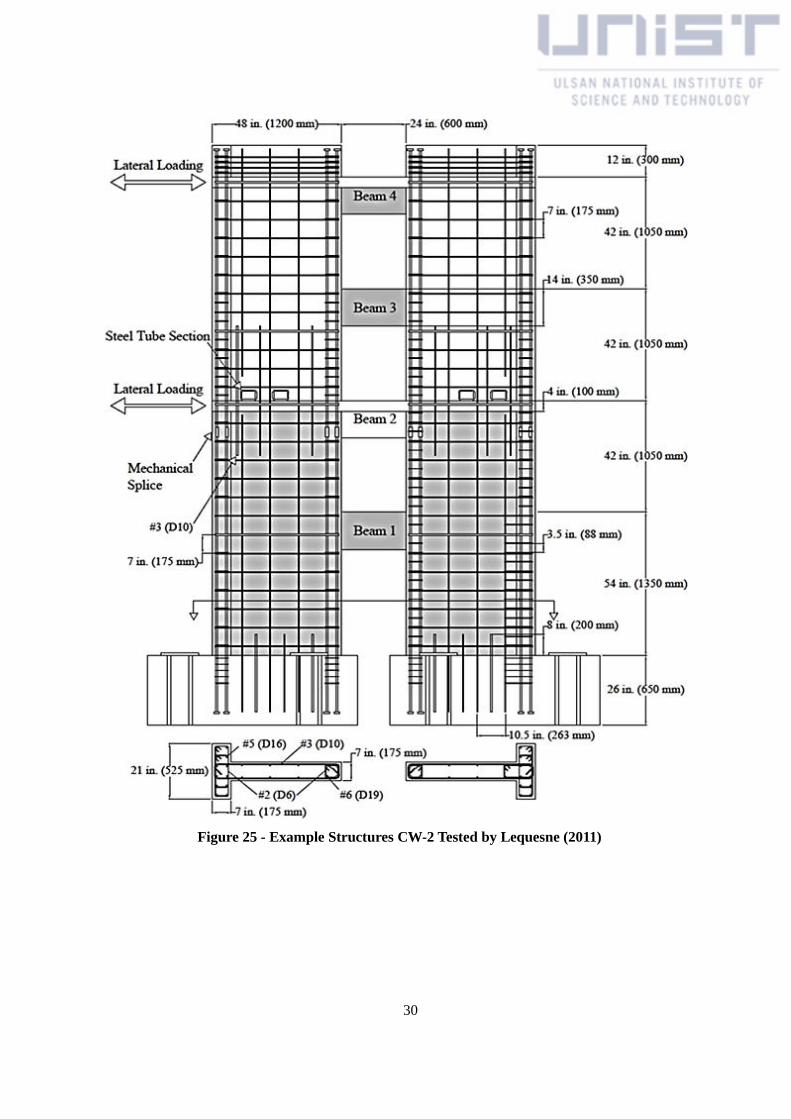
modeling methods. Confinement with shear reinforcement can lead to some difficulties in

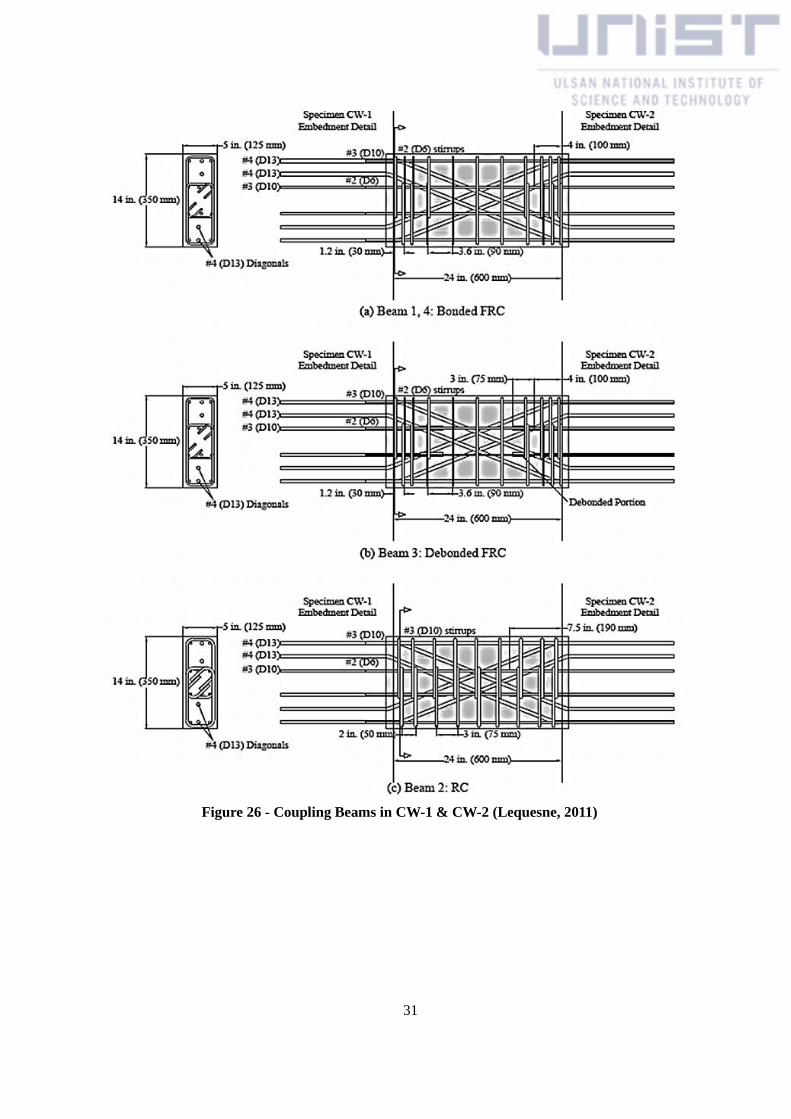
construction work. Instead of this, the use of HPFRCCs can reduce these troubles because the fibers

impede the crack opening of concrete and improve the tensional behavior of concrete like the

confinement effect. This paper studied the impact that the ductility exhibited by HPFRCCs

components in the critical regions has on the system performance. For this purpose, there are

approximately 1/3 scale two specimens (CW-1 and CW-2) applied cyclic displacement reversals

(Figure 27) on 4th floor. Both four-story specimens consisted of two T-shaped reinforced walls, four

precast coupling beams, and slabs at the second and forth levels. The dimension and details of the

specimen are shown in Figure 24 and Figure 25. The shaded areas in these figures were constructed

with HPFRCCs. The coupling beams of the example structures designed diagonal reinforcement to

prevent sliding shear failures and ensure ductile behavior. Figure 26 shows the dimension and details

of the diagonal reinforced coupling beams with an angle of approximately 28˚.

The differences between CW-1 and CW-2 specimens are shown in Table 5. The main difference

is the material used at the first two stories of each wall. Instead of normal concrete in CW-1,

HPFRCCs were used in CW-2. The wall details of CW-1 designed in accordance with ACI Building

Code 318-08. The first two stories of CW-2 wall were made with HPFRCCs, and designed with a

higher concrete shear stress contribution. Therefore, reduced amount of vertical and confinement

reinforcement was designed. Another difference about detailing is that the dowel bars at the base of

CW-2 were designed to supplement the flexural reinforcement at the cold joint. The longitudinal

reinforcements of CW-1 coupling beams were terminated in the wall by 75 mm from the beam-to-wall

interface. Because this made the damage localization at the interface, there was limited the ability of

coupled effect. The CW-2 had the fully developed coupling beam reinforcement.

This RC coupled wall tested the used the conventional concrete, and the results of concrete

material tests are shown in Table 6. Another material HPFRCCs was the mixture of concrete with

randomly distributed fibers. Table 7 shows the average results of HPFRCCs properties from the

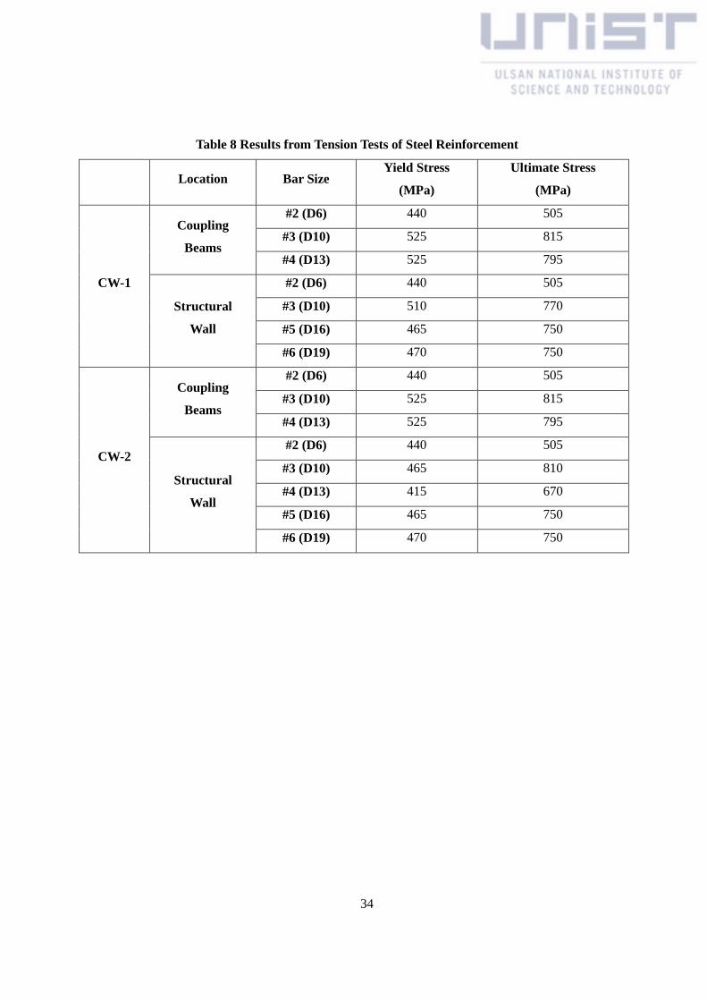
cylinders test. Grade 60 mild-steel properties are shown in Table 8.

29

Figure 24 - Example Structures CW-1 Tested by Lequesne (2011)

30

Figure 25 - Example Structures CW-2 Tested by Lequesne (2011)

31

Figure 26 - Coupling Beams in CW-1 & CW-2 (Lequesne, 2011)

32

Figure 27 - Cyclic Loading History (Lequesne, 2011)

Table 5 Test Variables in Two Specimens

Variation CW-1 CW-2

Material

of first two stories of walls Normal concrete HPFRCCs

Reinforcement

in first two stories of walls

Designed & detailed to satisfy

Chapter 21 of ACI 318-08

Reduced confinement

reinforcement for boundary

elements & vertical

reinforcement

Dowel bars at base X Placed at wall-to-foundation

Interface along the cold joint

Horizontal reinforcement

in coupling beams

Terminated in the walls by

only 3 in. from the interface Fully developed into the walls

33

Table 6 Properties of Normal Concrete

Location of Pour Specified f’c

(MPa)

28-Day f’c

(MPa)

Test Day f’c

(MPa)

CW-1

Beam-2 41.0 37.0 68.0

Foundation 28.0 34.0 53.0

Wall 1st story 28.0 37.0 48.0

Wall 2nd story 28.0 28.0 46.0

Slab #1 28.0 25.0 37.0

Wall 3rd story 28.0 38.0 46.0

Wall 4th story 28.0 48.0 66.0

Slab #2 28.0 51.0 66.0

Wall 5th story 28.0 46.0 61.0

CW-2

Beam-2 41.0 46.0 63.0

Foundation 28.0 50.0 52.0

Slab #1 28.0 41.0 46.0

Wall 3rd story 28.0 54.0 57.0

Wall 4th story 28.0 45.0 48.0

Slab #2 28.0 50.0 53.0

Wall 5th story 28.0 53.0 56.0

Table 7 Properties of HPFRCCs

Location of Pour

28-Day Tests

Test Day f'c

(MPa) f'c

(MPa)

ASTM 1609 Flexural Tests

σfc

(MPa)

σpeak

(MPa)

σ(δ=L/600)

(MPa)

σ(δ=L/150)

(MPa)

CW-1

Beam-1 38.0 4.90 7.10 6.70 3.60 71.0

Beam-3 38.0 4.90 7.10 6.70 3.60 71.0

Beam-4 41.0 5.70 7.70 7.20 4.10 74.0

CW-2

Beam-1 41.0 5.70 7.70 7.20 4.10 72.0

Beam-3 38.0 4.90 7.10 6.70 3.60 72.0

Beam-4 41.0 5.70 7.70 7.20 4.10 72.0

Wall 1st Story 50.0 5.50 7.50 7.20 5.10 51.0

Wall 2nd Story 46.0 5.80 7.20 7.00 3.90 50.0

34

Table 8 Results from Tension Tests of Steel Reinforcement

Location Bar Size Yield Stress

(MPa)

Ultimate Stress

(MPa)

CW-1

Coupling

Beams

#2 (D6) 440 505

#3 (D10) 525 815

#4 (D13) 525 795

Structural

Wall

#2 (D6) 440 505

#3 (D10) 510 770

#5 (D16) 465 750

#6 (D19) 470 750

CW-2

Coupling

Beams

#2 (D6) 440 505

#3 (D10) 525 815

#4 (D13) 525 795

Structural

Wall

#2 (D6) 440 505

#3 (D10) 465 810

#4 (D13) 415 670

#5 (D16) 465 750

#6 (D19) 470 750

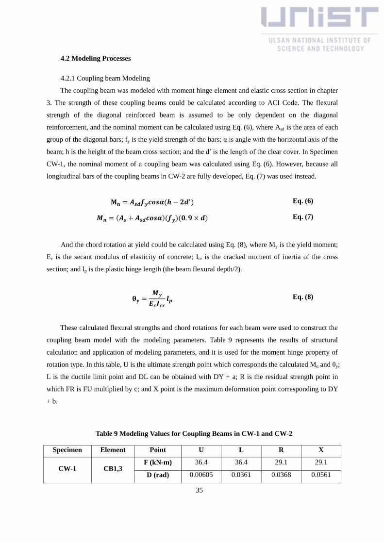
35

4.2 Modeling Processes

4.2.1 Coupling beam Modeling

The coupling beam was modeled with moment hinge element and elastic cross section in chapter

3. The strength of these coupling beams could be calculated according to ACI Code. The flexural

strength of the diagonal reinforced beam is assumed to be only dependent on the diagonal

reinforcement, and the nominal moment can be calculated using Eq. (6), where Asd is the area of each

group of the diagonal bars; fy is the yield strength of the bars; α is angle with the horizontal axis of the

beam; h is the height of the beam cross section; and the d’ is the length of the clear cover. In Specimen

CW-1, the nominal moment of a coupling beam was calculated using Eq. (6). However, because all

longitudinal bars of the coupling beams in CW-2 are fully developed, Eq. (7) was used instead.

𝐌𝐧 = 𝑨𝒔𝒅𝒇𝒚𝒄𝒐𝒔𝜶(𝒉 − 𝟐𝒅′) Eq. (6)

𝑴𝒏 = (𝑨𝒔 + 𝑨𝒔𝒅𝒄𝒐𝒔𝜶)(𝒇𝒚)(𝟎. 𝟗 × 𝒅) Eq. (7)

And the chord rotation at yield could be calculated using Eq. (8), where My is the yield moment;

Ec is the secant modulus of elasticity of concrete; Icr is the cracked moment of inertia of the cross

section; and lp is the plastic hinge length (the beam flexural depth/2).

𝛉𝐲 =𝑴𝒚

𝑬𝒄𝑰𝒄𝒓𝒍𝒑 Eq. (8)

These calculated flexural strengths and chord rotations for each beam were used to construct the

coupling beam model with the modeling parameters. Table 9 represents the results of structural

calculation and application of modeling parameters, and it is used for the moment hinge property of

rotation type. In this table, U is the ultimate strength point which corresponds the calculated Mn and θy;

L is the ductile limit point and DL can be obtained with DY + a; R is the residual strength point in

which FR is FU multiplied by c; and X point is the maximum deformation point corresponding to DY

+ b.

Table 9 Modeling Values for Coupling Beams in CW-1 and CW-2

Specimen Element Point U L R X

CW-1 CB1,3 F (kN-m) 36.4 36.4 29.1 29.1

D (rad) 0.00605 0.0361 0.0368 0.0561

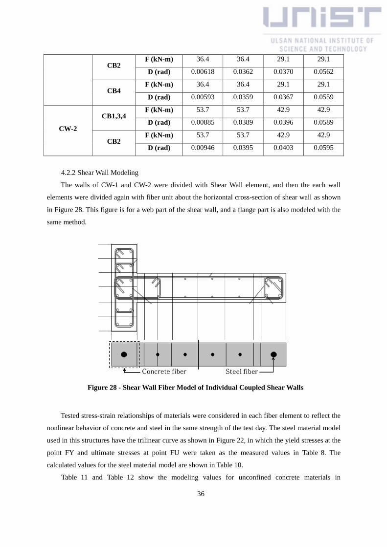
36

CB2 F (kN-m) 36.4 36.4 29.1 29.1

D (rad) 0.00618 0.0362 0.0370 0.0562

CB4 F (kN-m) 36.4 36.4 29.1 29.1

D (rad) 0.00593 0.0359 0.0367 0.0559

CW-2

CB1,3,4 F (kN-m) 53.7 53.7 42.9 42.9

D (rad) 0.00885 0.0389 0.0396 0.0589

CB2 F (kN-m) 53.7 53.7 42.9 42.9

D (rad) 0.00946 0.0395 0.0403 0.0595

4.2.2 Shear Wall Modeling

The walls of CW-1 and CW-2 were divided with Shear Wall element, and then the each wall

elements were divided again with fiber unit about the horizontal cross-section of shear wall as shown

in Figure 28. This figure is for a web part of the shear wall, and a flange part is also modeled with the

same method.

Figure 28 - Shear Wall Fiber Model of Individual Coupled Shear Walls

Tested stress-strain relationships of materials were considered in each fiber element to reflect the

nonlinear behavior of concrete and steel in the same strength of the test day. The steel material model

used in this structures have the trilinear curve as shown in Figure 22, in which the yield stresses at the

point FY and ultimate stresses at point FU were taken as the measured values in Table 8. The

calculated values for the steel material model are shown in Table 10.

Table 11 and Table 12 show the modeling values for unconfined concrete materials in

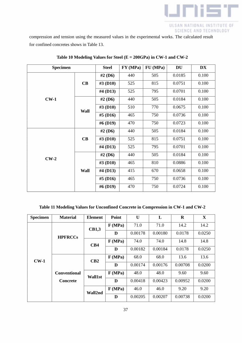
37

compression and tension using the measured values in the experimental works. The calculated result

for confined concretes shows in Table 13.

Table 10 Modeling Values for Steel (E = 200GPa) in CW-1 and CW-2

Specimen Steel FY (MPa) FU (MPa) DU DX

CW-1

CB

#2 (D6) 440 505 0.0185 0.100

#3 (D10) 525 815 0.0751 0.100

#4 (D13) 525 795 0.0701 0.100

Wall

#2 (D6) 440 505 0.0184 0.100

#3 (D10) 510 770 0.0675 0.100

#5 (D16) 465 750 0.0736 0.100

#6 (D19) 470 750 0.0723 0.100

CW-2

CB

#2 (D6) 440 505 0.0184 0.100

#3 (D10) 525 815 0.0751 0.100

#4 (D13) 525 795 0.0701 0.100

Wall

#2 (D6) 440 505 0.0184 0.100

#3 (D10) 465 810 0.0886 0.100

#4 (D13) 415 670 0.0658 0.100

#5 (D16) 465 750 0.0736 0.100

#6 (D19) 470 750 0.0724 0.100

Table 11 Modeling Values for Unconfined Concrete in Compression in CW-1 and CW-2

Specimen Material Element Point U L R X

CW-1

HPFRCCs

CB1,3 F (MPa) 71.0 71.0 14.2 14.2

D 0.00178 0.00180 0.0178 0.0250

CB4 F (MPa) 74.0 74.0 14.8 14.8

D 0.00182 0.00184 0.0178 0.0250

Conventional

Concrete

CB2 F (MPa) 68.0 68.0 13.6 13.6

D 0.00174 0.00176 0.00708 0.0200

Wall1st F (MPa) 48.0 48.0 9.60 9.60

D 0.00418 0.00423 0.00952 0.0200

Wall2nd F (MPa) 46.0 46.0 9.20 9.20

D 0.00205 0.00207 0.00738 0.0200

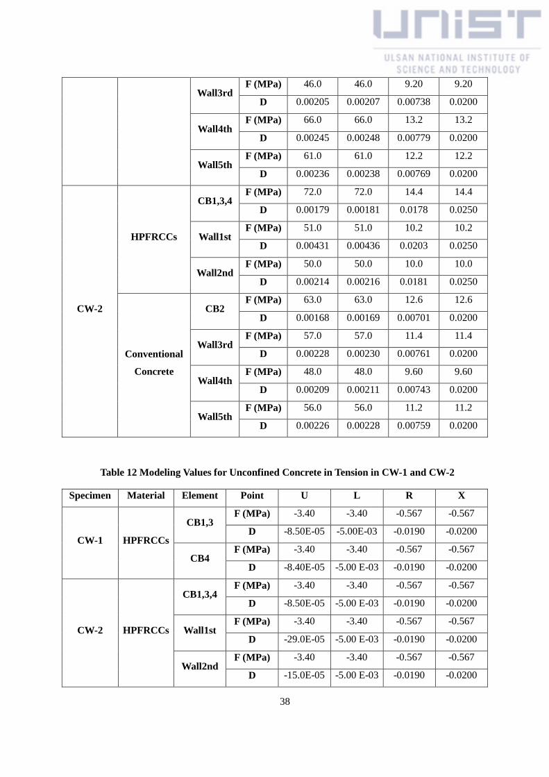
38

Wall3rd F (MPa) 46.0 46.0 9.20 9.20

D 0.00205 0.00207 0.00738 0.0200

Wall4th F (MPa) 66.0 66.0 13.2 13.2

D 0.00245 0.00248 0.00779 0.0200

Wall5th F (MPa) 61.0 61.0 12.2 12.2

D 0.00236 0.00238 0.00769 0.0200

CW-2

HPFRCCs

CB1,3,4 F (MPa) 72.0 72.0 14.4 14.4

D 0.00179 0.00181 0.0178 0.0250

Wall1st F (MPa) 51.0 51.0 10.2 10.2

D 0.00431 0.00436 0.0203 0.0250

Wall2nd F (MPa) 50.0 50.0 10.0 10.0

D 0.00214 0.00216 0.0181 0.0250

Conventional

Concrete

CB2 F (MPa) 63.0 63.0 12.6 12.6

D 0.00168 0.00169 0.00701 0.0200

Wall3rd F (MPa) 57.0 57.0 11.4 11.4

D 0.00228 0.00230 0.00761 0.0200

Wall4th F (MPa) 48.0 48.0 9.60 9.60

D 0.00209 0.00211 0.00743 0.0200

Wall5th F (MPa) 56.0 56.0 11.2 11.2

D 0.00226 0.00228 0.00759 0.0200

Table 12 Modeling Values for Unconfined Concrete in Tension in CW-1 and CW-2

Specimen Material Element Point U L R X

CW-1 HPFRCCs

CB1,3 F (MPa) -3.40 -3.40 -0.567 -0.567

D -8.50E-05 -5.00E-03 -0.0190 -0.0200

CB4 F (MPa) -3.40 -3.40 -0.567 -0.567

D -8.40E-05 -5.00 E-03 -0.0190 -0.0200

CW-2 HPFRCCs

CB1,3,4 F (MPa) -3.40 -3.40 -0.567 -0.567

D -8.50E-05 -5.00 E-03 -0.0190 -0.0200

Wall1st F (MPa) -3.40 -3.40 -0.567 -0.567

D -29.0E-05 -5.00 E-03 -0.0190 -0.0200

Wall2nd F (MPa) -3.40 -3.40 -0.567 -0.567

D -15.0E-05 -5.00 E-03 -0.0190 -0.0200

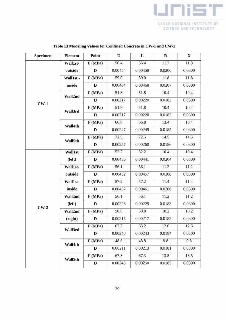
39

Table 13 Modeling Values for Confined Concrete in CW-1 and CW-2

Specimen Element Point U L R X

CW-1

Wall1st-

outside

F (MPa) 56.4 56.4 11.3 11.3

D 0.00454 0.00458 0.0206 0.0300

Wall1st -

inside

F (MPa) 59.0 59.0 11.8 11.8

D 0.00464 0.00468 0.0207 0.0300

Wall2nd F (MPa) 51.8 51.8 10.4 10.4

D 0.00217 0.00220 0.0182 0.0300

Wall3rd F (MPa) 51.8 51.8 10.4 10.4

D 0.00217 0.00220 0.0182 0.0300

Wall4th F (MPa) 66.8 66.8 13.4 13.4

D 0.00247 0.00249 0.0185 0.0300

Wall5th F (MPa) 72.5 72.5 14.5 14.5

D 0.00257 0.00260 0.0186 0.0300

CW-2

Wall1st

(left)

F (MPa) 52.2 52.2 10.4 10.4

D 0.00436 0.00441 0.0204 0.0300

Wall1st-

outside

F (MPa) 56.1 56.1 11.2 11.2

D 0.00452 0.00457 0.0206 0.0300

Wall1st-

inside

F (MPa) 57.2 57.2 11.4 11.4

D 0.00457 0.00461 0.0206 0.0300

Wall2nd

(left)

F (MPa) 56.1 56.1 11.2 11.2

D 0.00226 0.00229 0.0183 0.0300

Wall2nd

(right)

F (MPa) 50.8 50.8 10.2 10.2

D 0.00215 0.00217 0.0182 0.0300

Wall3rd F (MPa) 63.2 63.2 12.6 12.6

D 0.00240 0.00243 0.0184 0.0300

Wall4th F (MPa) 48.8 48.8 9.8 9.8

D 0.00211 0.00213 0.0181 0.0300

Wall5th F (MPa) 67.3 67.3 13.5 13.5

D 0.00248 0.00250 0.0185 0.0300

40

4.3 Correlationship of Modeling Results and Experimental Results

Figure 29 and Figure 30 show the result of overturning moment-wall drift relationship for CW-1

and CW-2 respectively. A solid line is the experimental result, and a dotted line is the modeling result.

The proposed modeling methods well represent the overall behavior of the tested couple shear wall

systems such as the strength, stiffness, and energy dissipation. The analysis well simulates strength

increase observed in the measured strength of CW-2 by using HPFRCCs in comparison with CW-1. In

the modeling results, although the initial strengths of both specimens are similar with the experimental

result, the strengths after yielding have slightly different values. In the experiments, the slabs part of

the beams at the second and forth levels were shown to develop reinforcement yielding and contribute

to the coupling of the walls, which was not considered in the modeling. These could affect the smaller

overturning moments. The modeling results couldn’t express the strength reductions which were

occurred after 2% wall drift. the sliding shear displacement of coupling beam at 2nd

and 3rd

floor was

occurred in CW-1 during 2% wall drift and shear fail of the wall in CW-2 at -2.5% wall drift.

The stiffnesses of the tested specimen were well represented by the modeling results, and energy

dissipations were also well fitted with somewhat exaggeration by the overestimated strengths after 2%

wall drift. The amount energy degradation is related with the stiffness degradation in the hysteresis.

The reduction of stiffness of walls can be reflected with the application of energy dissipation factors,

and the shape of hysteresis loop is controlled by the unloading behavior. In this modeling, the

minimum unloading elastic range is used.

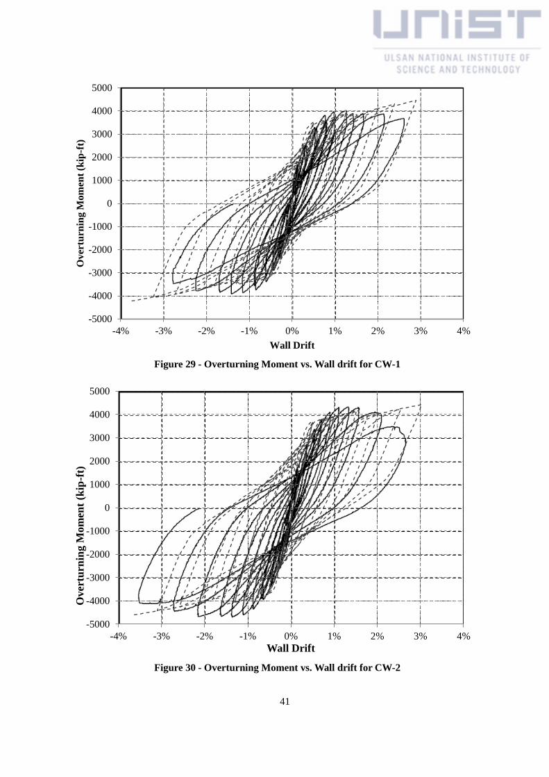
41

Figure 29 - Overturning Moment vs. Wall drift for CW-1

Figure 30 - Overturning Moment vs. Wall drift for CW-2

-5000

-4000

-3000

-2000

-1000

0

1000

2000

3000

4000

5000

-4% -3% -2% -1% 0% 1% 2% 3% 4%

Ov

ertu

rnin

g M

om

ent

(kip

-ft)

Wall Drift

-5000

-4000

-3000

-2000

-1000

0

1000

2000

3000

4000

5000

-4% -3% -2% -1% 0% 1% 2% 3% 4%

Over

turn

ing M

om

ent

(kip

-ft)

Wall Drift

42

Stain gauges were placed on the reinforcement throughout the CW-1 and CW-2, and this can be

compared through the steel material strain capacity in wall and beam element result. In case of CW-1,

the yield strains prior to 0.5% wall drift were observed in the all coupling beams and first floor of wall.

The most of the first floor reinforcements in walls were yielded at 1.0% wall drift, and additional

diagonal reinforcements in beams were also yielded in this drift. After 1.0% to end of test, the rest of

flexure reinforcements in first floor wall almost yielded. The analyses well simulated that the all

coupling beams first reached the yield moment at about 0.5% wall drift as shown in Figure 31, and the

walls developed yield strains at the partial first story prior to 0.5% wall drift. The yield stains of all

the first floor walls were observed during the 1.25% wall drift cycle.

By the experimental work of CW-2, the first yield strain was measured at the reinforcements in

all coupling beams and first floor wall prior to 0.5% wall drift like as CW-1. When the CW-2 was

pushed with 1.0% wall drift, the yield strains throughout the first floor walls were occurred. In

contrast with CW-1, the horizontal reinforcements in the first floor wall were yielded prior to end of

the test. This means that after ductile flexure behavior, the shear failure at approximately 2.5% wall

drift. In the results of the CW-2 modeling, the yielding of coupling beams (Figure 32) and first partial

floor walls were well modeled prior to 0.5% wall drift. When the wall drift was 1.25%, all first floor

walls reached the yield strains. However, because the model of CW-2 was assumed to flexure

behavior, the shear failure at 2.5% wall drift shown in the experiment could not be simulated.

Figure 31 - Coupling Beams of CW-1

43

Figure 32 - Coupling Beams of CW-2

44

Chapter 5. Analysis of a Tall Building with Coupled Shear Walls

5.1 Example Structures

The previous coupled wall examples were used to assess the proposed modeling methods. The

purpose of the modeling in this chapter is to apply the modeling methods to a tall building and

examine the behavior of the buildings depending on the use of the HPFRCs. The actual residential 56-

story building (TB-1 and TB-2) was selected for nonlinear analysis using the proposed modeling

methods. Figure 33 shows the plane view of this tall building and the labels are represented for the

structural components of a core wall system. In the seismic design of building frame systems, the

shear core is assumed to resist all of the lateral loads. Therefore, only the core wall system was

modelled for the efficient analysis and the stiffness and strength of the columns were ignored to

examine the response of the tall building under lateral loads.

Figure 33 - Plane View of the Tall Building

45

The core system consisted of 3-type coupling beams and 16-types of reinforced concrete walls,

and the average story height is 3m. The cross sections of coupling beams in the tall buildings are

shown in Figure 34. The all of the horizontal bars used in coupling beams are D19, and the all of

stirrups used in coupling beams are D13 with the different spacing; 100mm for (a), (b), and (c),

150mm for (d), (e), and (g), and 250mm for (f).

Figure 34 - Cross Sections of CBs in Tall Buildings (unit: mm)

Table 14 shows the reinforcement of the walls, where tw means the thickness of each walls, V,Bar

is the information of vertical reinforcement, H,Bar is the information of horizontal reinforcement, and

E,Bar is the information of the vertical reinforcement at the both end zones of the wall (Figure 35).

The concrete strengths for the modeling are 50MPa from 1F to 10F, 45MPa from 11F to 20F, and

35MPa from 21F to 56F for vertical members in the example buildings. The concrete strengths of

horizontal members are assumed 1.4 times smaller than the materials of vertical members. The yield

strengths have 400MPa for lower than D13 steel, and 600MPa for more than D16 steel. While the all

structure members of the TB-1 are made of RC, the TB-2 has all HPFRCCs coupling beams and

HPFRCCs walls from bottom to 14th floor (1/4 stories of the wall to cover the plastic hinge enough).

46

Figure 35 - Cross Section of Walls in Tall Buildings

Table 14 Reinforcement of Walls in TB-1 and TB-2 (unit: mm)

CW1 CW6

Strory tW V,Bar H,Bar E,Bar Strory tW V,Bar H,Bar E,Bar

51F~56F 600 D13

@300

D13

@200 4-D19 50F~56F 400

D10

@300

D13

@300 4-D13

49F~50F 600 D16

@250

D16

@250 4-D19 33F~49F 550

D10

@200

D13

@200 4-D13

2F~48F 600 D13

@300

D13

@200 4-D19 31F~32F 550

D16

@200

D16

@200 4-D19

1F 1000 D16

@300

D16

@190 4-D19 29F~30F 550

D16

@250

D16

@250 4-D19

CW1A 4F~28F 550 D10

@200

D13

@200 4-D13

Strory tW V,Bar H,Bar E,Bar 2F~3F 550 D16

@300

D13

@200 4-D19

51F~56F 600 D13

@250

D13

@200 4-D16 1F 900

D19

@200

D19

@250 4-D22

49F~50F 600 D16

@300

D16

@250 4-D19 CW6A

29F~48F 600 D13

@300

D13

@200 4-D16 Strory tW V,Bar H,Bar E,Bar

27F~28F 600 D16

@200

D16

@250 4-D19 50F~56F 550

D10

@200

D13

@200 4-D13

3F~26F 600 D13

@300

D13

@200 4-D16 33F~49F 550

D10

@200

D13

@200 4-D13

1F~2F 1000 D16

@300

D16

@190 4-D19 31F~32F 550

D16

@200

D16

@200 4-D19

47

CW2 29F~30F 550 D16

@250

D16

@250 4-D19

Strory tW V,Bar H,Bar E,Bar 4F~28F 550 D10

@200

D13

@200 4-D13

55F~56F 600 D13

@250

D13

@200 4-D16 2F~3F 550

D16

@300

D13

@200 4-D19

32F~54F 600 D13

@300

D13

@200 4-D16 1F 900

D19

@250

D19

@250 6-D22

30F~31F 600 D16

@250

D16

@250 4-D19 CW7

2F~29F 600 D13

@300

D13

@200 4-D16 Strory tW V,Bar H,Bar E,Bar

1F 1000 D16

@300

D16

@190 4-D19 50F~56F 400

D10

@300

D13

@300 4-D13

CW3 34F~49F 550 D10

@200

D13

@200 4-D13

Strory tW V,Bar H,Bar E,Bar 28F~33F 550 D16

@250

D16

@250 4-D19

32F~56F 600 D13

@300

D13

@200 4-D16 6F~27F 550

D10

@200

D13

@200 4-D13

30F~31F 600 D16

@250

D16

@250 4-D19 2F~5F 550

D16

@250

D16

@250 6-D19

2F~29F 600 D13

@300

D13

@200 4-D16 1F 900

D19

@100

D19

@250 10-D22

1F 1000 D16

@300

D16

@190 4-D19 CW8

CW3A Strory tW V,Bar H,Bar E,Bar

Strory tW V,Bar H,Bar E,Bar 54F~56F 550 D16

@250

D13

@200 4-D13

32F~56F 600 D13

@300

D13

@200 4-D16 32F~53F 550

D10

@200

D13

@200 4-D16

30F~31F 600 D16

@300

D16

@250 4-D19 30F~31F 550

D16

@250

D16

@250 4-D19

19F~29F 600 D13

@300

D13

@200 4-D16 7F~29F 550

D10

@200

D13

@200 4-D13

17F-1F~18F 600 D16

@300

D16

@250 4-D19 5F~6F 550

D16

@250

D16

@250 4-D19

2F~17F 600 D13

@300

D13

@200 4-D19 2F~4F 550

D16

@250

D16

@250 6-D19

48

1F 1000 D16

@250

D16

@190 6-D19 1F 900

D19

@100

D19

@250 10-D22

CW4 W1

Strory tW V,Bar H,Bar E,Bar Strory tW V,Bar H,Bar E,Bar

32F~56F 600 D13

@300

D13

@200 4-D16 56F 400

D13

@200

D13

@300 4-D16

30F~31F 600 D16

@250

D16

@250 4-D19 31F~55F 400

D10

@300

D13

@300 4-D13

25F~29F 600 D13

@300

D13

@200 4-D16 17F-1F~30F 400

D13

@250

D13

@250 4-D16

2F~24F 600 D16

@250

D16

@250 4-D22 4F~17F 400

D10

@200

D13

@300 4-D13

1F 1000 D19

@200

D19

@200 6-D22 2F~3F 400

D16

@300

D13

@300 4-D19

CW4A 1F 400 D19

@150

D16

@300 6-D22

Strory tW V,Bar H,Bar E,Bar W2

56F 600 D16

@250

D16

@250 4-D19 Strory tW V,Bar H,Bar E,Bar

50F~55F 600 D13

@300

D13

@200 4-D16 31F~56F 250

D10

@450

D10

@280 4-D13

31F~49F 600 D16

@250

D16

@250 4-D19 29F~30F 250

D13

@200

D10

@200 4-D16

29F~30F 600 D19

@120

D16

@250 4-D22 20F~28F 250

D10

@450

D10

@280 4-D13

2F~28F 600 D16

@250

D16

@250 4-D19 18F~19F 250

D10

@200

D10

@200 4-D13

1F 1000 D19

@250

D19

@190 6-D22 8F~17F-1F 250

D10

@450

D10

@280 4-D13

CW5 2F~7F 250 D10

@200

D10

@200 4-D13

Strory tW V,Bar H,Bar E,Bar 1F 250 D13

@300

D10

@220 4-D16

50F~56F 600 D10

@250

D13

@250 4-D16 W2A

31F~49F 600 D13

@300

D13

@190 4-D16 Strory tW V,Bar H,Bar E,Bar

49

29F~30F 600 D16

@250

D16

@250 4-D19 31F~56F 350

D10

@300

D10

@200 4-D13

2F~28F 600 D13

@250

D13

@190 4-D19 30F 350

D13

@200

D13

@250 4-D16

1F 1000 D16

@250

D16

@250 4-D22 2F~29F 350

D10

@300

D10

@200 4-D16

※ Size of Reinforcements

Bar Diameter (mm) Area (mm2)

D10 9.53 71.3

D13 12.7 126.7

D16 15.9 198.6

D19 19.1 286.5

D22 22.2 387.1

D25 25.4 506.7

1F 350 D13

@200

D13

@250 4-D19

W3

Strory tW V,Bar H,Bar E,Bar

31F~56F 250 D10

@450

D10

@280 4-D13

30F 250 D10

@200

D10

@200 4-D16

2F~29F 250 D10

@450

D10

@280 4-D16

1F 250 D13

@300

D13

@250 4-D19

50

5.2 Modeling Processes

In this example of a tall building, the modeling process for coupling beams and shear walls was

same with the previous example.

5.2.1 Coupling Beam Modeling

The coupling beams are expected to develop flexural yielding at their both ends. Therefore, the

model of the coupling beam also consists of a ‘Moment Hinge of Rotation Type’ on each end and an

‘Elastic Beam Section’ as same with the previous example. The elastic beam section also has the

0.20EcIg effective elastic stiffness to include slip/extension effects. The calculated nominal moment

and yield rotation values were used for the moment hinge model with the ASCE/SEI 41-06 parameter

(Table 4) to construct the backbone curves (Figure 18). The flexural strength of the conventional

reinforced beams is calculated using Eq. (9), where As is the area of tension bars; fy is the yield

strength of the bars; d is the distance from extreme compression fiber to centroid of longitudinal

tension reinforcements, a is the depth of equivalent rectangular stress block in compression zone of

the cross section, and (d-a/2) is the moment arm. And the chord rotation at yield could be calculated

using Eq. (6). Table 15 shows modeling values for coupling beams that used the results of structural

calculation and application of modeling parameters in the same way of the previous example.

𝐌𝐧 = 𝑨𝒔𝒇𝒚(𝒅 − 𝒂/𝟐) Eq. (9)

Table 15 Modeling Values for Coupling Beams in TB-1 and TB-2

Specimen Element Floor Point U L R X

TB-1

CB1-1

1F~10F F (kN-m) 1370 1370 687 687

D (rad) 0.00890 0.0289 0.0295 0.0439

11F~17F F (kN-m) 1360 1360 678 678

D (rad) 0.00936 0.0294 0.0299 0.0444

18F~20F F (kN-m) 1190 1190 596 596

D (rad) 0.00814 0.0281 0.0287 0.0431

21F~40F F (kN-m) 1160 1160 578 578

D (rad) 0.00917 0.0292 0.0298 0.0442

41F~56F F (kN-m) 996 996 498 498

D (rad) 0.00778 0.0278 0.0283 0.0428

CB1-2 1F~10F F (kN-m) 1370 1370 1030 1030

D (rad) 0.00545 0.0305 0.0311 0.0555

51

11F~17F F (kN-m) 1360 1360 1020 1020

D (rad) 0.00573 0.0307 0.0313 0.0557

18F~20F F (kN-m) 1190 1190 894 894

D (rad) 0.00499 0.0300 0.0306 0.0550

21F~40F F (kN-m) 1160 1160 867 867

D (rad) 0.00562 0.0306 0.0312 0.0556

41F~56F F (kN-m) 996 996 747 747

D (rad) 0.00477 0.0298 0.0304 0.0548

CB1-3

1F~10F F (kN-m) 1370 1370 687 687

D (rad) 0.00782 0.0278 0.0284 0.0428

11F~17F F (kN-m) 1360 1360 678 678

D (rad) 0.00823 0.0282 0.0288 0.0432

18F~20F F (kN-m) 1190 1190 894 894

D (rad) 0.00715 0.0322 0.0328 0.0572

21F~40F F (kN-m) 1160 1160 867 867

D (rad) 0.00806 0.0331 0.0337 0.0581

41F~56F F (kN-m) 996 996 498 498

D (rad) 0.00684 0.0268 0.0274 0.0418

CB2-1

1F~10F F (kN-m) 801 801 400 400

D (rad) 0.00786 0.0279 0.0284 0.0429

11F~17F F (kN-m) 792 792 396 396

D (rad) 0.00827 0.0283 0.0288 0.0433

18F~20F F (kN-m) 612 612 459 459

D (rad) 0.00630 0.0313 0.0319 0.0563

21F~30F F (kN-m) 598 598 449 449

D (rad) 0.00710 0.0321 0.0327 0.0571

31F~56F F (kN-m) 520 520 260 260

D (rad) 0.00611 0.0261 0.0266 0.0411

CB2-2

1F~10F F (kN-m) 801 801 400 400

D (rad) 0.0140 0.0340 0.0347 0.0490

11F~17F F (kN-m) 792 792 396 396

D (rad) 0.0148 0.0348 0.0355 0.0498

18F~20F F (kN-m) 612 612 306 306

D (rad) 0.0113 0.0312 0.0319 0.0462

52

21F~30F F (kN-m) 598 598 299 299

D (rad) 0.0127 0.0327 0.0333 0.0477

31F~56F F (kN-m) 520 520 260 260

D (rad) 0.0109 0.0309 0.0315 0.0459

CB3

1F~10F F (kN-m) 397 397 198 198

D (rad) 0.00723 0.0272 0.0278 0.0422

11F~20F F (kN-m) 392 392 294 294

D (rad) 0.00760 0.0326 0.0333 0.0576

21F~56F F (kN-m) 380 380 285 285

D (rad) 0.00856 0.0336 0.0342 0.0586

TB-2

CB1-1

1F~10F F (kN-m) 1650 1650 824 824

D (rad) 0.0107 0.0578 0.0590 0.0878

11F~17F F (kN-m) 1630 1630 813 813

D (rad) 0.0112 0.0587 0.0599 0.0887

18F~20F F (kN-m) 1430 1430 715 715

D (rad) 0.00981 0.0563 0.0574 0.0863

21F~40F F (kN-m) 1390 1390 693 693

D (rad) 0.0108 0.0583 0.0595 0.0883

41F~56F F (kN-m) 1200 1200 597 597

D (rad) 0.00929 0.0556 0.0567 0.0856

CB1-2

1F~10F F (kN-m) 1650 1650 1240 1240

D (rad) 0.00657 0.0609 0.0621 0.111

11F~17F F (kN-m) 1630 1630 1220 1220

D (rad) 0.00684 0.0615 0.0627 0.111

18F~20F F (kN-m) 1430 1430 1073 1073

D (rad) 0.00601 0.0600 0.0612 0.110

21F~40F F (kN-m) 1390 1390 1040 1040

D (rad) 0.00661 0.0612 0.0625 0.111

41F~56F F (kN-m) 1190 1190 896 896

D (rad) 0.00569 0.0595 0.0607 0.110

CB1-3

1F~10F F (kN-m) 1650 1650 824 824

D (rad) 0.00942 0.0556 0.0568 0.0856

11F~17F F (kN-m) 1630 1630 813 813

D (rad) 0.00981 0.0565 0.0576 0.0865

53

18F~20F F (kN-m) 1430 1430 1070 1070

D (rad) 0.00862 0.0643 0.0656 0.114

21F~40F F (kN-m) 1390 1390 1040 1040

D (rad) 0.00948 0.0661 0.0674 0.116

41F~56F F (kN-m) 1190 1190 597 597

D (rad) 0.00817 0.0537 0.0548 0.0837

CB2-1

1F~10F F (kN-m) 961 961 480 480

D (rad) 0.00956 0.0557 0.0568 0.0857

11F~17F F (kN-m) 951 951 475 475

D (rad) 0.00997 0.0565 0.0577 0.0865

18F~20F F (kN-m) 734 734 551 551

D (rad) 0.00770 0.0626 0.0638 0.113

21F~30F F (kN-m) 718 718 538 538

D (rad) 0.00854 0.0642 0.0655 0.114

31F~56F F (kN-m) 624 624 312 312

D (rad) 0.00741 0.0522 0.0533 0.0822

CB2-2

1F~10F F (kN-m) 961 961 480 480

D (rad) 0.0171 0.0681 0.0694 0.0981

11F~17F F (kN-m) 951 951 475 475

D (rad) 0.0178 0.0695 0.0709 0.0995

18F~20F F (kN-m) 734 734 367 367

D (rad) 0.0137 0.0625 0.0637 0.0925

21F~30F F (kN-m) 718 718 359 359

D (rad) 0.0152 0.0654 0.0667 0.0954

31F~56F F (kN-m) 624 624 312 312

D (rad) 0.0132 0.0618 0.0630 0.0918

CB3

1F~10F F (kN-m) 476 476 238 238

D (rad) 0.00878 0.0545 0.0555 0.0845

11F~20F F (kN-m) 471 471 353 353

D (rad) 0.00915 0.0652 0.0665 0.115

21F~56F F (kN-m) 456 456 342 342

D (rad) 0.0101 0.0671 0.0685 0.117

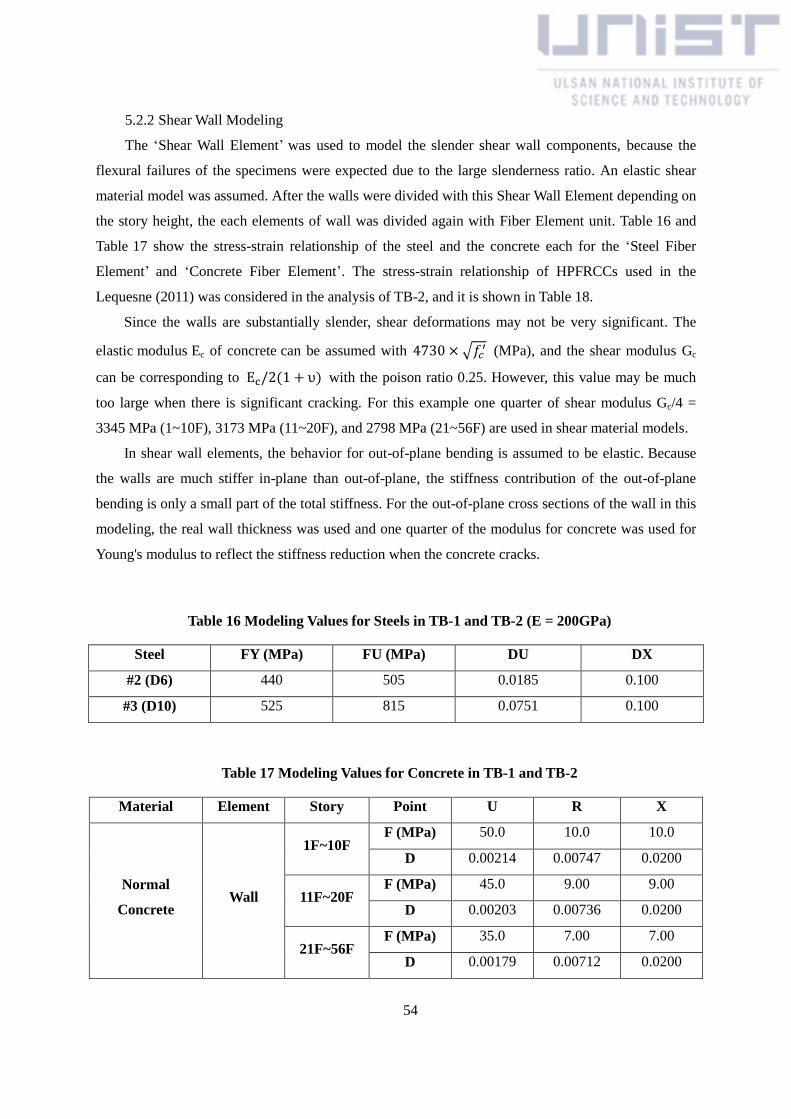
54

5.2.2 Shear Wall Modeling

The ‘Shear Wall Element’ was used to model the slender shear wall components, because the

flexural failures of the specimens were expected due to the large slenderness ratio. An elastic shear

material model was assumed. After the walls were divided with this Shear Wall Element depending on

the story height, the each elements of wall was divided again with Fiber Element unit. Table 16 and

Table 17 show the stress-strain relationship of the steel and the concrete each for the ‘Steel Fiber

Element’ and ‘Concrete Fiber Element’. The stress-strain relationship of HPFRCCs used in the

Lequesne (2011) was considered in the analysis of TB-2, and it is shown in Table 18.

Since the walls are substantially slender, shear deformations may not be very significant. The

elastic modulus Ec of concrete can be assumed with 4730 × √𝑓𝑐′ (MPa), and the shear modulus Gc

can be corresponding to Ec/2(1 + υ) with the poison ratio 0.25. However, this value may be much

too large when there is significant cracking. For this example one quarter of shear modulus Gc/4 =

3345 MPa (1~10F), 3173 MPa (11~20F), and 2798 MPa (21~56F) are used in shear material models.

In shear wall elements, the behavior for out-of-plane bending is assumed to be elastic. Because

the walls are much stiffer in-plane than out-of-plane, the stiffness contribution of the out-of-plane

bending is only a small part of the total stiffness. For the out-of-plane cross sections of the wall in this

modeling, the real wall thickness was used and one quarter of the modulus for concrete was used for

Young's modulus to reflect the stiffness reduction when the concrete cracks.

Table 16 Modeling Values for Steels in TB-1 and TB-2 (E = 200GPa)

Steel FY (MPa) FU (MPa) DU DX

#2 (D6) 440 505 0.0185 0.100

#3 (D10) 525 815 0.0751 0.100

Table 17 Modeling Values for Concrete in TB-1 and TB-2

Material Element Story Point U R X

Normal

Concrete Wall

1F~10F F (MPa) 50.0 10.0 10.0

D 0.00214 0.00747 0.0200

11F~20F F (MPa) 45.0 9.00 9.00

D 0.00203 0.00736 0.0200

21F~56F F (MPa) 35.0 7.00 7.00

D 0.00179 0.00712 0.0200

55

Beam

1F~10F F (MPa) 35.7 7.14 7.14

D 0.00842 0.0138 0.0200

11F~20F F (MPa) 32.1 6.43 6.43

D 0.00799 0.0133 0.0200

21F~56F F (MPa) 25.0 5.00 5.00

D 0.00705 0.0124 0.0200

Table 18 Modeling Values for HPFRCCs in TB-2

Compression

Material Story Point U R X

HPFRCCs

1F~10F F (MPa) 50.0 10.0 10.0

D 0.00150 0.0175 0.0200

11F~14F F (MPa) 45.0 9.00 9.00

D 0.00142 0.0174 0.0200

Tension

HPFRCCs 1F~14F F (MPa) 3.40 0.570 0.570

D 0.00405 0.0190 0.0200

5.2.3 Floor Slab and Columns

The floor slab is modeled as a rigid diaphragm using the slaving constraints, and the masses are

lumped at each floor. The center of mass and the gravity load on the each wall from one floor slab

were calculated using SAP2000 software. After modeling the one story of the tall building example

through the SAP2000, the approximate results of translational and rotational masses (Table 19) could

be applied to the center of mass.

Table 19 Results of Lumped Masses at each floor of Tall Building

Area A (m2) 692.2

Moment of inertia I22 (m

4) 48100

I33 (m4) 61100

Dead Load (kN/m2) 20.7

Translational weight (kN) 14300

Rotational weight (kN-m2) 2260000

56

(kN-mm2) 2.26E+12

Although P-Δ effects can be considered in wall elements, this model used the "P-Δ column"

elements. When the local buckling failure of the wall is occurred by the weak out-of-plane strength of

wall, the structure model can no longer support the gravity loads, and the analysis do not have the

solution. To prevent this error, the P-Δ column was considered at the center of mass with elastic

‘Simple Bar’ elements. P-Δ effects are considered through only this column. The gravity loads of each

floor were applied this column with the slaving constraint. The mechanism of the P-Δ column is

shown in the Figure 36. When the axial load P is applied to the column and there is horizontal load H

in this structure, the effective shear force PΔ/h is occurred at this column. By the equilibrium, the

shear force in the wall sections is equal to H + PΔ/h. In addition, the accidental torsion for P-Δ effects

can be modeled whit the other P-Δ column at the eccentric location.

Figure 36 - Mechanism of P- Δ Column

5.2.4 Loads

For the gravity loads modeling, the dead loads (DL) include the self-weight of the floor slabs

which is calculated with the weight density of materials and superimposed loads (1kN/m2). The

design live load (LL) is 2kN/m2 on the slabs. All floors were assumed to have same dead and live load,

and the gravity loads of slabs were applied at the center of mass as mentioned above. However, the

wall has different behavior depending on the existence of the vertical compression due to the delay of

crack. Because the floor slabs of this example are not modeled, properly estimated gravity loads from

slab to wall should be applied directly to the nodes of the core wall system. SAP2000 was used again

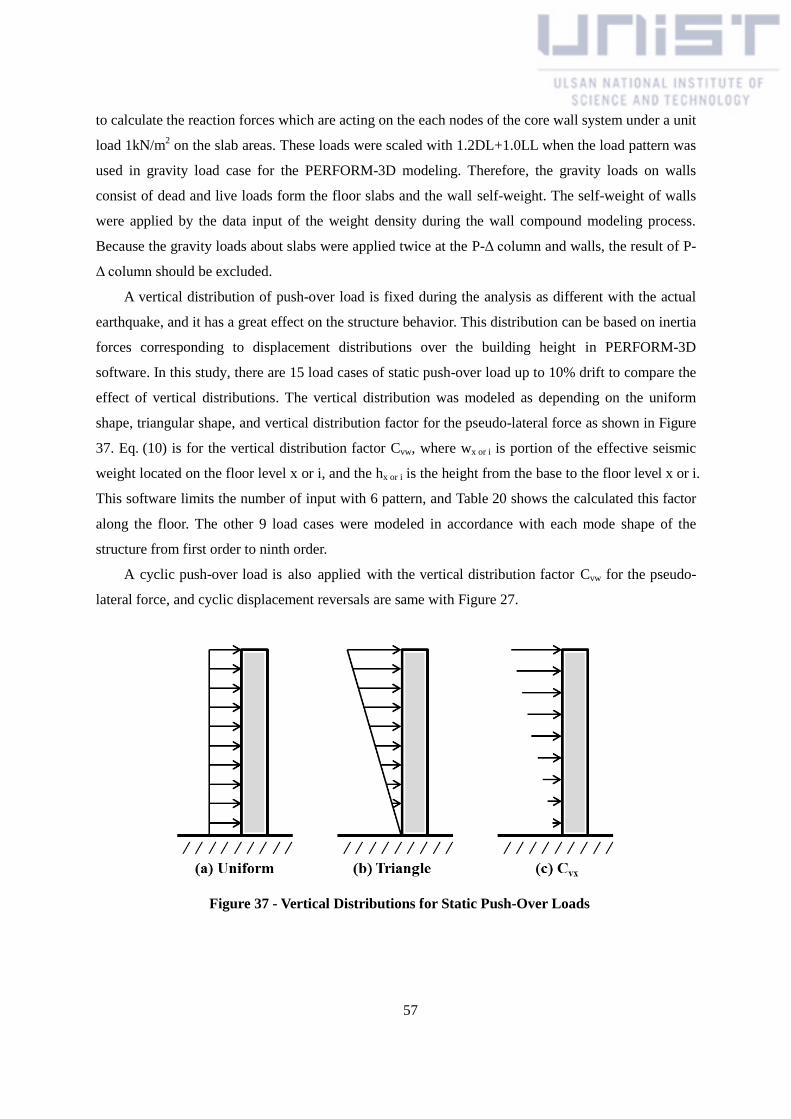
57

to calculate the reaction forces which are acting on the each nodes of the core wall system under a unit

load 1kN/m2 on the slab areas. These loads were scaled with 1.2DL+1.0LL when the load pattern was

used in gravity load case for the PERFORM-3D modeling. Therefore, the gravity loads on walls

consist of dead and live loads form the floor slabs and the wall self-weight. The self-weight of walls

were applied by the data input of the weight density during the wall compound modeling process.

Because the gravity loads about slabs were applied twice at the P-Δ column and walls, the result of P-

Δ column should be excluded.

A vertical distribution of push-over load is fixed during the analysis as different with the actual

earthquake, and it has a great effect on the structure behavior. This distribution can be based on inertia

forces corresponding to displacement distributions over the building height in PERFORM-3D

software. In this study, there are 15 load cases of static push-over load up to 10% drift to compare the

effect of vertical distributions. The vertical distribution was modeled as depending on the uniform

shape, triangular shape, and vertical distribution factor for the pseudo-lateral force as shown in Figure

37. Eq. (10) is for the vertical distribution factor Cvw, where wx or i is portion of the effective seismic

weight located on the floor level x or i, and the hx or i is the height from the base to the floor level x or i.

This software limits the number of input with 6 pattern, and Table 20 shows the calculated this factor

along the floor. The other 9 load cases were modeled in accordance with each mode shape of the

structure from first order to ninth order.

A cyclic push-over load is also applied with the vertical distribution factor Cvw for the pseudo-

lateral force, and cyclic displacement reversals are same with Figure 27.

Figure 37 - Vertical Distributions for Static Push-Over Loads

58

𝑪𝒗𝒙 =𝒘𝒙𝒉𝒙

𝒌

∑ 𝒘𝒊𝒉𝒊𝒌𝒏

𝒊=𝟏

Eq. (10)

Table 20 Vertical Distribution Factor Cvw in TB-1 and TB-2

Floor hi (mm) Cvx

0 0 0

10 36100 0.0192

20 72400 0.0760

30 105700 0.1604

40 135800 0.2632

56 184300 0.4812

In this study, a dynamic earthquake load case was applied to compare and observe the nonlinear

seismic behavior. For this nonlinear time history analysis, a ground motion considered for an

earthquake that is El Centro earthquake at California (1940). This typical earthquake is known as the

first recorded major earthquake and the time history of acceleration records is shown in Figure 38.

The total duration is 29 seconds and the maximum acceleration is 0.32g. This earthquake load

analysis was modeled with 5% Rayleigh damping.

Figure 38 - El Centro Earthquake

-0.4

-0.3

-0.2

-0.1

0

0.1

0.2

0.3

0.4

0 5 10 15 20 25 30 35

Acc

. (g

)

Time (s)

59

5.3 Analysis Results

5.3.1 Mode Property

When the masses of the tall buildings are defined, PERFORM-3D calculates the mode properties

which are about mode shape and periods. The mode shapes are calculated to characterize

displacement patterns in elastic state. In the push-over analysis, the structures commonly have

fundamental mode dominant behavior. The effective mass factor represents the significant of the each

mode, and the mode with higher effective mass factors has the relatively higher participation to the

structural response under the seismic load. Mode shapes of TB-1 and TB-2 is shown in Figure 39 and

Figure 40 respectively, and the each period for these models is expressed in Table 21 and Table 22.

TB-1 and TB-2 have large torsional mode shapes due to the irregularity and both models have similar

mode shapes except the 3rd

, 5th, and 9

th modes. The 5

th and 9

th mode shapes of TB-2 behave in the

opposite direction with TB-1, and the 3rd

mode shape of TB-2 seems to have smaller torsional

behavior than that of TB-1. The periods and effective mass factors of each mode are almost similar in

both models.

Figure 39 - Mode Shape of TB-1

Table 21 Mode Periods of TB-1

Mode Period (s) Effective Mass Factor

H1 H2

1 7.42 0.39 2.23E-05

2 6.45 0.0473 0.546

Mode 1 Mode 2 Mode 3 Mode 4 Mode 5 Mode 6 Mode 7 Mode 8 Mode 9

60

3 6.14 0.222 0.121

4 2.06 0.0110 4.45E-04

5 1.57 0.154 0.0198

6 1.51 0.0173 0.161

7 1.10 0.00184 1.92E-04

8 0.73 0.00168 8.34E-05

9 0.70 0.0349 0.0270

Figure 40 - Mode Shape of TB-2

Table 22 Mode Periods of TB-2

Mode Period (s) Effective Mass Factors

H1 H2

1 7.41 0.390 2.59E-05

2 6.45 0.0491 0.541

3 6.15 0.221 0.125

4 2.06 0.0104 4.41E-04

5 1.57 0.155 0.0191

6 1.51 0.0167 0.162

7 1.10 0.00171 1.84E-04

8 0.73 0.00163 4.44E-05

9 0.70 0.0350 0.0271

Mode 1 Mode 2 Mode 3 Mode 4 Mode 5 Mode 6 Mode 7 Mode 8 Mode 9

61

5.3.2 Push-Over Load

This section shows the results when the tall building is under various push-over loads in H1

direction. The strain gages were placed at the tips of the each wall element to check the yield of

vertical reinforcement and compression level when concrete begins to lose strength. When the hinges

form, a substantial yield of the reinforcement would be measured.

5.3.2.1 Story Drift

Figure 41, Figure 42, and Figure 43 show the interstory drift result of the two models depending

on the vertical patterns of the static push-over load case. When both models are under the uniform and

triangular load distribution up to 10% roof drift, they behave with almost same story drift way. The

large story drift was occurred in 2nd

and 3rd

floors. However, the result of TB-2 under the Cvx factor

pattern shows different with the other profiles of story drift. The large story drift occurred at 15th floor,

and this means the week story was shifted by using HPFRCCs.

Figure 41 - Story Drift under Static Push-Over Loads with Uniform Distribution

0

10

20

30

40

50

60

-5% 0% 5% 10% 15%

Flo

or

Story Drift

TB-1,H1

TB-1,H2

TB-2,H1

TB-2,H2

62

Figure 42 - Story Drift under Static Push-Over Loads with Triangular Distribution

Figure 43 - Story Drift under Static Push-Over Loads with C Factor Distribution

0

10

20

30

40

50

60

-5% 0% 5% 10% 15%

Flo

or

Story Drift

TB-1,H1

TB-1,H2

TB-2,H1

TB-2,H2

0

10

20

30

40

50

60

-10% 0% 10% 20%

Flo

or

Story Drift

TB-1,H1

TB-1,H2

TB-2,H1

TB-2,H2

63

Figure 44 shows the interstory drift results at 10% roof drift depending on the vertical patterns

that were modeled with the mode shapes of TB-1 and TB-2 from 1st mode to 9

th mode. The results

from first to fourth mode have similar. The relatively large story drifts were developed at 2nd

and 3rd

floors of both TB-1 and TB-2 in positive H1 direction. The results with 5th mode and 6

th mode vertical

distribution are also similar, and both TB-1 and TB-2 have large story drifts at 34th and 35

th floors in

negative H1 direction. When the vertical distribution was 7th mode shape, the result show large story

drift occurred from 23rd

floor to 25th floor in negative H1 direction. In case of 8

th mode distribution,

the sustainable story drift was developed from 41st floor to 44

th floor in positive H1 direction. The

result with 9th mode distribution also shows the large story drift at the upper part of the structures from

40th floor to 43

rd floor in positive H1 direction.

Figure 45 shows the story drift of TB-1 and TB-2 under the cyclic load with Cvx factor

distribution. At the initial cycles with 0.25% roof drift, the two models behaved with similar story

drift. When the target roof drift of TB-1 reached at 1.5% drift, the story drift of 5th floor began to

rapidly increase. At this cycle, the 4th and 5

th floors of CW3 and CW3A wall showed yield stains in

tension and the CW6A strain gage at the 4th floor reached at the DX state in compression. From this to

3.0% roof drift cycle, the TB-1 behaved with large story drift at 4th and 5

th floor. The final result of

this model shows that the 2nd

and 3rd

floor had large story drift in H2 direction which suddenly began

from the -3.0% target drift cycle as shown in the figure. At the final cycle, the compression strain

gages reached DX at the 2nd

floor of CW1 and CW1A and it would have made the large H2 story drift.

In the case of TB-2, the weak story occurred at 15th and 16

th floors from 1% roof drift. The a

number of 15th floor strain gages indicated yield strains in tension and several compression strains of

the walls reached at the DX level. The story drift in H2 direction began to sharply increased at 15th

and 16th floors when 3% roof drift, and t at 3.5% roof drift, this model finally indicated a brittle

fracture behavior and was stopped as the H2 story drift reached to 10%. These would be related to the

measurement of all strain gages at 15th floor without the CW8 that indicated at the maximum

deformation point.

TB-1 had a plastic hinge in lower stories and the use of HPFRCCs moved it to upper stories

which used the normal concrete. At the later stage, the large displacement in H2 direction was shown

in the both models even though the load direction is just H1.

64

Figure 44 - Story Drift under Static Push-Over Loads with Mode Shape Distribution

0

10

20

30

40

50

60

-10% 0% 10% 20%

Flo

or

Story Drift

Mode1

0

10

20

30

40

50

60

-10% 0% 10% 20%F

loor

Story Drift

Mode2

0

10

20

30

40

50

60

-10% 0% 10% 20%

Flo

or

Story Drift

Mode3

0

10

20

30

40

50

60

-40%-20% 0% 20%

Flo

or

Story Drift

Mode5

0

10

20

30

40

50

60

-10% 0% 10% 20%

Flo

or

Story Drift

Mode4

0

10

20

30

40

50

60

-40%-20% 0% 20%

Flo

or

Story Drift

Mode6

0

10

20

30

40

50

60

-20%-10% 0% 10%

Flo

or

Story Drift

Mode7

0

10

20

30

40

50

60

0% 20% 40%

Flo

or

Story Drift

Mode9

0

10

20

30

40

50

60

0% 50%

Flo

or

Story Drift

Mode8

TB-1,H1 TB-1,H2

TB-2,H1 TB-2,H2

65

Figure 45 - Story Drift under Cyclic Push-Over Loads with C-factor Distribution

0

10

20

30

40

50

60

0.0% 0.2% 0.4%

Flo

or

Story Drift

0.25%

0

10

20

30

40

50

60

-1% 0% 1% 2%F

loor

Story Drift

1.0%

0

10

20

30

40

50

60

-2% 0% 2%

Flo

or

Story Drift

1.25%

0

10

20

30

40

50

60

-2% 0% 2% 4%

Flo

or

Story Drift

1.5%

0

10

20

30

40

50

60

-2% 0% 2% 4%

Flo

or

Story Drift

2.0%

0

10

20

30

40

50

60

-5% 0% 5%

Flo

or

Story Drift

2.5%

0

10

20

30

40

50

60

-5% 0% 5%

Flo

or

Story Drift

3.0%

0

10

20

30

40

50

60

-5% 0% 5%

Flo

or

Story Drift

-3.0%

TB-1,H1 TB-1,H2

TB-2,H1 TB-2,H2

0

10

20

30

40

50

60

-10% 0% 10%20%

Flo

or

Story Drift

3.5%

66

5.3.2.2 Base Shear

Figure 46 shows the relationship between base shear and roof drift when the static push-over

loads are applied without the gravity load. U, T, and C in the legend of this figure represent the

vertical patterns of lateral loads; uniform, triangular, and Cvx factor distribution respectively. TB-1 and

TB-2 models with uniform distribution had largest base shear and stiffness, followed by the triangular

distribution cases. TB-2 model indicate the increased base shear and stiffness responses compared

with TB-1. However, a relatively larger strength reduction occurred in TB-2 model at lower roof drift

than TB-1 case. The reason of a little strength reduction in TB-1 model was that the compressive stain

at 5th floor of CW6A exceeded the defined maximum deformation that means the corresponding fiber

element could not resist applied loads anymore. It also occurred at the 15th

floor of CW6A in TB-2

model at the earlier roof drift.

Figure 47 shows the base shear results when TB-1 is subjected to the static push-over loads up to

10% roof drift without gravity and the load has vertical distributions with mode shapes. The relations

of the base shear and roof drift from 1st mode to 3

rd mode distribution show same result and the

strength and stiffness are much smaller than that of the other modes. The 8th mode case has the largest

stiffness, and the 9th mode has the largest strength.

The same load cases were applied to TB-2, and the results about the base shear are shown in

Figure 48. The results of TB-2 from 1st mode to 3

rd mode distribution are the same and the strength

and stiffness are even smaller than the values from the other load cases such as TB-1 results. The

result with 4th mode distribution shows the sustainable large strength in a moment before 1% roof drift.

And the largest stiffness was modeled when 8th mode distribution case. The overall strength and

stiffness of TB-2 were not much different from TB-1 except for 4th mode case in spite of the use of

HPFRCCs. The base shear result under the load with Cvx factor distribution is similar with the result

with 1st mode to 3

rd mode distribution.

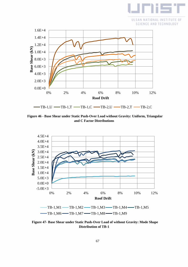
67

Figure 46 - Base Shear under Static Push-Over Load without Gravity: Uniform, Triangular

and C Factor Distributions

Figure 47- Base Shear under Static Push-Over Load of without Gravity: Mode Shape

Distribution of TB-1

0.0E+0

2.0E+3

4.0E+3

6.0E+3

8.0E+3

1.0E+4

1.2E+4

1.4E+4

1.6E+4

0% 2% 4% 6% 8% 10% 12%

Base

Sh

ear

(kN

)

Roof Drift

TB-1,U TB-1,T TB-1,C TB-2,U TB-2,T TB-2,C

-5.0E+3

0.0E+0

5.0E+3

1.0E+4

1.5E+4

2.0E+4

2.5E+4

3.0E+4

3.5E+4

4.0E+4

4.5E+4

0% 2% 4% 6% 8% 10% 12%

Base

Sh

ear

(kN

)

Roof Drift

TB-1,M1 TB-1,M2 TB-1,M3 TB-1,M4 TB-1,M5

TB-1,M6 TB-1,M7 TB-1,M8 TB-1,M9

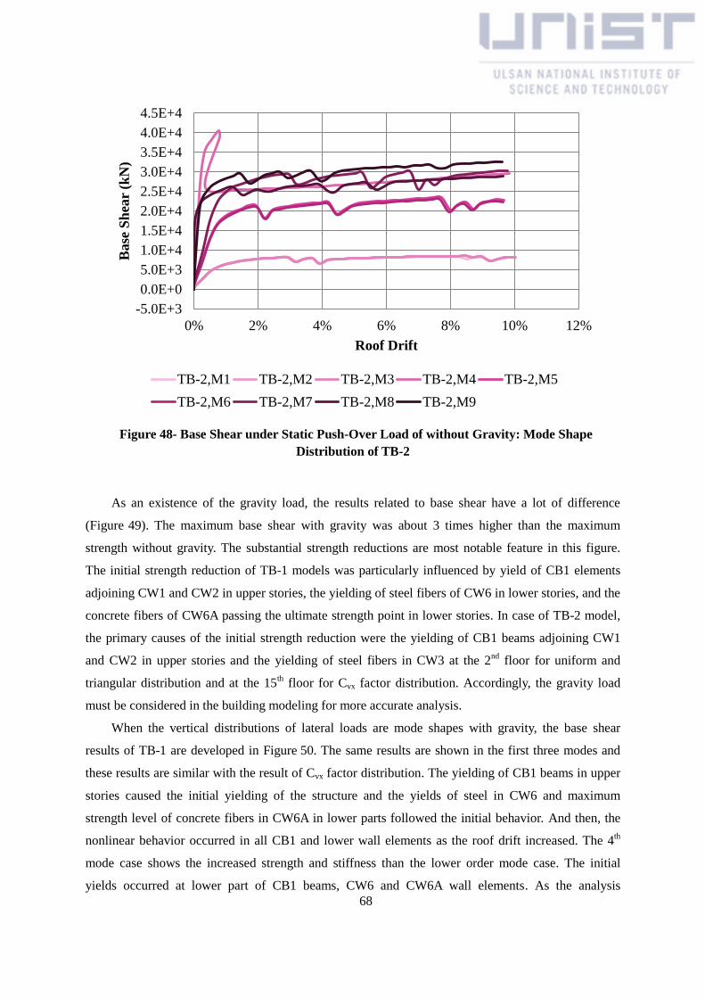
68

Figure 48- Base Shear under Static Push-Over Load of without Gravity: Mode Shape

Distribution of TB-2

As an existence of the gravity load, the results related to base shear have a lot of difference

(Figure 49). The maximum base shear with gravity was about 3 times higher than the maximum

strength without gravity. The substantial strength reductions are most notable feature in this figure.

The initial strength reduction of TB-1 models was particularly influenced by yield of CB1 elements

adjoining CW1 and CW2 in upper stories, the yielding of steel fibers of CW6 in lower stories, and the

concrete fibers of CW6A passing the ultimate strength point in lower stories. In case of TB-2 model,

the primary causes of the initial strength reduction were the yielding of CB1 beams adjoining CW1

and CW2 in upper stories and the yielding of steel fibers in CW3 at the 2nd

floor for uniform and

triangular distribution and at the 15th floor for Cvx factor distribution. Accordingly, the gravity load

must be considered in the building modeling for more accurate analysis.

When the vertical distributions of lateral loads are mode shapes with gravity, the base shear

results of TB-1 are developed in Figure 50. The same results are shown in the first three modes and

these results are similar with the result of Cvx factor distribution. The yielding of CB1 beams in upper

stories caused the initial yielding of the structure and the yields of steel in CW6 and maximum

strength level of concrete fibers in CW6A in lower parts followed the initial behavior. And then, the

nonlinear behavior occurred in all CB1 and lower wall elements as the roof drift increased. The 4th

mode case shows the increased strength and stiffness than the lower order mode case. The initial

yields occurred at lower part of CB1 beams, CW6 and CW6A wall elements. As the analysis

-5.0E+3

0.0E+0

5.0E+3

1.0E+4

1.5E+4

2.0E+4

2.5E+4

3.0E+4

3.5E+4

4.0E+4

4.5E+4

0% 2% 4% 6% 8% 10% 12%

Ba

se S

hea

r (k

N)

Roof Drift

TB-2,M1 TB-2,M2 TB-2,M3 TB-2,M4 TB-2,M5

TB-2,M6 TB-2,M7 TB-2,M8 TB-2,M9

69

progressed the nonlinear behavior was developed at the wall elements in the middle stories and all

beams elements. In case of 5th mode distribution, the result reached at the maximum strength level as

CW1 elements in upper stories and CW6A in 33rd

floor yielded. The strength reductions were

progressed by the nonlinear behavior of wall elements in middle stories. And the structures were

failed in the negative H1 direction at these stories. The similar behavior was shown in 6th mode shape

case. When the load with 7th mode shape distribution was applied, the result of TB-1 shows the largest

strength in early roof drift. The initial nonlinear behavior was due to the yielding of CW1-1L in upper

and lower stories, the yields of steel fibers at CW6A, and the excess of ultimate compressive strength

point of CW6 from 21st floor to 26

th floor. The failures of CB1 beams from 21

st floor occurred and the

wall elements failed in the middle stories. The 8th mode case shows the main nonlinear behavior at the

upper stories around 40th floor wall and beam elements in positive H1 direction, and the 9

th mode case

also had the main local behavior at around 40th floor with higher strength than the 8

th mode result.

Figure 51 demonstrates the base shear result of TB-2 according to load case with the mode shape

distribution after gravity load was applied. The first three mode cases show a similar behavior that

have the initial yield by the yields of steel fibers in CW6 at 15th floor. The following nonlinear

behavior occurred at CB1 beams and the wall elements around 15th floor and lower parts. The main

reason of the final failure was the fails of the wall elements at 2nd

floor. The 4th mode case has the

increase strength and stiffness values. The initial nonlinear behavior of the model is due to the yield of

beam elements, the yield of CW6 elements, and the passing ultimate strength of concrete fiber in

CW6A at lower stories. After the progressing nonlinear behavior of lower wall elements, the

continuous nonlinear behavior occurred at wall elements around 30th floor and all CB1 elements. The

5th mode and 6

th mode cases show similar responses that have the large nonlinear behavior at around

33rd

floor in negative H1 direction. When the vertical distribution was in accordance with 7th mode

shape, the result shows the largest strength and stiffness. The main nonlinear behavior occurred at the

walls and beams upper 21st floor in negative H1 direction. In case of the 8

th mode and 9

th mode

distributions, the local behavior of TB-2 model is similar with TB-1.

70

Figure 49 - Base Shear under Static Push-Over Load with Gravity: Uniform, Triangular and C

Factor Distributions

Figure 50- Base Shear under Static Push-Over Load with Gravity: Mode Shape Distribution of

TB-1

-2.0E+4

-1.0E+4

0.0E+0

1.0E+4

2.0E+4

3.0E+4

4.0E+4

5.0E+4

0% 2% 4% 6% 8% 10% 12%

Base

Sh

ear

(kN

)

Roof Drift

TB-1,U TB-1,T TB-1,C TB-2,U TB-2,T TB-2,C

-6.0E+4

-4.0E+4

-2.0E+4

0.0E+0

2.0E+4

4.0E+4

6.0E+4

8.0E+4

1.0E+5

0% 2% 4% 6% 8% 10% 12%

Base

Sh

ear

(kN

)

Roof Drift

TB-1,M1 TB-1,M2 TB-1,M3 TB-1,M4 TB-1,M5

TB-1,M6 TB-1,M7 TB-1,M8 TB-1,M9

71

Figure 51- Base Shear under Static Push-Over Load with Gravity: Mode Shape Distribution of

TB-2

The comparison of hysteretic behavior between two models is shown in Figure 52. The

maximum strength of TB-2 was increased by the use of HPFRCCs. However, while TB-1 models

maintained the maximum strength from 0.75% to 1.5%, the initial strength reduction of TB-2

occurred at 1.12% drift just as soon as the base shear reached the maximum strength. Furthermore,

although the ductile property of HPFRCCs, the large strength reduction of TB-2 occurred when the

target drift cycle was 2.5% as different with TB-1 model in positive direction. At that drift, the axial

strain gages at 15th floor in CW3 and CW3A reached the tensile yield strain DY, and the compressive

stain in CW6A at same floor reached DR. The use of HPFRCCs from base to the 14th floor caused

rather large strain at the 15th floor. On the opposite direction, when the target drift was -2.5% drift,

TB-1 also showed a large strength reduction behavior as the compressive strain of CW3 and CW3A

exceeded the maximum deformation. Overall, if the shift of week story did not take place, the

behavior of TB-2 could be better than the TB-1. When applying HPFRCCs in the critical region of the

structural wall, the reduced reinforcement such as experimental work of Lequesne (2011) would be

expected to avoid this shift of weak stories as well as the efficiency of construction work.

-4.0E+4

-2.0E+4

0.0E+0

2.0E+4

4.0E+4

6.0E+4

8.0E+4

1.0E+5

0% 2% 4% 6% 8% 10% 12%

Ba

se S

hea

r (k

N)

Roof Drift

TB-2,M1 TB-2,M2 TB-2,M3 TB-2,M4 TB-2,M5

TB-2,M6 TB-2,M7 TB-2,M8 TB-2,M9

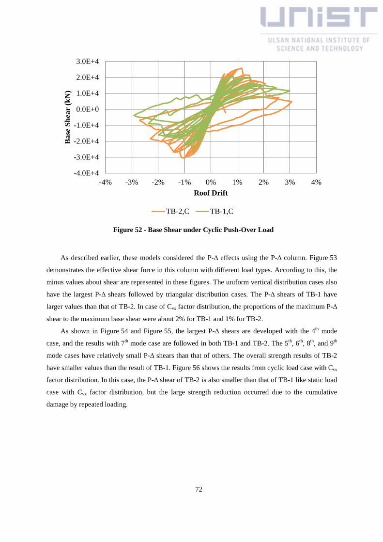
72

Figure 52 - Base Shear under Cyclic Push-Over Load

As described earlier, these models considered the P-Δ effects using the P-Δ column. Figure 53

demonstrates the effective shear force in this column with different load types. According to this, the

minus values about shear are represented in these figures. The uniform vertical distribution cases also

have the largest P-Δ shears followed by triangular distribution cases. The P-Δ shears of TB-1 have

larger values than that of TB-2. In case of Cvx factor distribution, the proportions of the maximum P-Δ

shear to the maximum base shear were about 2% for TB-1 and 1% for TB-2.

As shown in Figure 54 and Figure 55, the largest P-Δ shears are developed with the 4th mode

case, and the results with 7th mode case are followed in both TB-1 and TB-2. The 5

th, 6

th, 8

th, and 9

th

mode cases have relatively small P-Δ shears than that of others. The overall strength results of TB-2

have smaller values than the result of TB-1. Figure 56 shows the results from cyclic load case with Cvx

factor distribution. In this case, the P-Δ shear of TB-2 is also smaller than that of TB-1 like static load

case with Cvx factor distribution, but the large strength reduction occurred due to the cumulative

damage by repeated loading.

-4.0E+4

-3.0E+4

-2.0E+4

-1.0E+4

0.0E+0

1.0E+4

2.0E+4

3.0E+4

-4% -3% -2% -1% 0% 1% 2% 3% 4%

Ba

se S

hea

r (k

N)

Roof Drift

TB-2,C TB-1,C

73

Figure 53 - P-Δ Shear under Static Push-Over Load: Uniform, Triangular and C Factor

Distributions

Figure 54 - P-Δ Shear under Static Push-Over Load: Mode Shape Distribution of TB-1

-6.0E+2

-5.0E+2

-4.0E+2

-3.0E+2

-2.0E+2

-1.0E+2

0.0E+0

1.0E+2

0% 2% 4% 6% 8% 10% 12%

P-Δ

Sh

ear

(kN

)

Roof Drift

TB-1,U TB-1,T TB-1,C TB-2,U TB-2,T TB-2,C

-1.0E+3

-8.0E+2

-6.0E+2

-4.0E+2

-2.0E+2

0.0E+0

2.0E+2

4.0E+2

0% 2% 4% 6% 8% 10% 12%

P-Δ

Sh

ear

(kN

)

Roof Drift

TB-1,M1 TB-1,M2 TB-1,M3 TB-1,M4 TB-1,M5

TB-1,M6 TB-1,M7 TB-1,M8 TB-1,M9

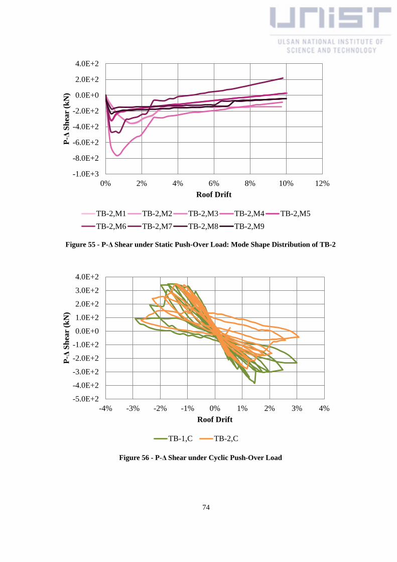
74

Figure 55 - P-Δ Shear under Static Push-Over Load: Mode Shape Distribution of TB-2

Figure 56 - P-Δ Shear under Cyclic Push-Over Load

-1.0E+3

-8.0E+2

-6.0E+2

-4.0E+2

-2.0E+2

0.0E+0

2.0E+2

4.0E+2

0% 2% 4% 6% 8% 10% 12%

P-Δ

Sh

ear

(kN

)

Roof Drift

TB-2,M1 TB-2,M2 TB-2,M3 TB-2,M4 TB-2,M5

TB-2,M6 TB-2,M7 TB-2,M8 TB-2,M9

-5.0E+2

-4.0E+2

-3.0E+2

-2.0E+2

-1.0E+2

0.0E+0

1.0E+2

2.0E+2

3.0E+2

4.0E+2

-4% -3% -2% -1% 0% 1% 2% 3% 4%

P-Δ

Sh

ear

(kN

)

Roof Drift

TB-1,C TB-2,C

75

5.3.2.3 Base Moment

The overturning moment result for TB-1 and TB-2 are shown in Figure 57 and Figure 60

according to the load type. The overall behavior is similar with base shear result, in which TB-2

model also has an increased strength about the overturning moment by using the HPFRCCs model.

However, the maximum strengths depending on the vertical distribution shows almost same values as

different with base shear results. TB-2 model has a relatively larger strength reduction than TB-1. The

overturning moment results under the cyclic push-over load case have similar result about the base

shear.

Figure 58 and Figure 59 show the results about the overturning moment of TB-1 and TB-2

respectively under the static push-over loads in accordance with the mode shapes. The largest

overturning moment was developed with the first three mode cases in both TB-1 and TB-2, and the

values are similar with the results from the uniform, triangular, and Cvx factor distribution cases. The

4th mode cases of both models also have the similar maximum strength values. However, the higher

mode cases show the relatively smaller values.

Figure 57 - Overturning Moment under Static Push-Over Load: Uniform, Triangular, and C

Factor Distributions

0.0E+0

5.0E+5

1.0E+6

1.5E+6

2.0E+6

2.5E+6

3.0E+6

3.5E+6

4.0E+6

4.5E+6

5.0E+6

0% 2% 4% 6% 8% 10% 12%

OT

M (

kN

-m)

Roof Drift

TB-1,U TB-1,T TB-1,C TB-2,U TB-2,T TB-2,C

76

Figure 58 - Overturning Moment under Static Push-Over Load: Mode Shape Distribution of

TB-1

Figure 59 - Overturning Moment under Static Push-Over Load: Mode Shape Distribution of

TB-2

-4.0E+6

-3.0E+6

-2.0E+6

-1.0E+6

0.0E+0

1.0E+6

2.0E+6

3.0E+6

4.0E+6

-2% 0% 2% 4% 6% 8% 10% 12%

OT

M (

kN

-m)

Roof Drift

TB-1,M1 TB-1,M2 TB-1,M3 TB-1,M4 TB-1,M5

TB-1,M6 TB-1,M7 TB-1,M8 TB-1,M9

-4.0E+6

-3.0E+6

-2.0E+6

-1.0E+6

0.0E+0

1.0E+6

2.0E+6

3.0E+6

4.0E+6

5.0E+6

-2% 0% 2% 4% 6% 8% 10% 12%

OT

M (

kN

-m)

Roof Drift

TB-2,M1 TB-2,M2 TB-2,M3 TB-2,M4 TB-2,M5

TB-2,M6 TB-2,M7 TB-2,M8 TB-2,M9

77

Figure 60 - Overturning Moment under Cyclic Push-Over Load

Figure 61 and Figure 64 represent the torsional moments of TB-1 and TB-2 under the static and

cyclic push-over load respectively. A relatively larger torsional moment was indicated in TB-2 than

TB-1, and the vertical pattern which has the largest torsional moment was the uniform distribution.

The uniform distribution was required to larger force to push the building structure up to same drift

ration with other vertical distribution, and this would cause larger torsion moment in same model. The

results about the torsional moment were inversely proportional to the base shear results, and TB-2 had

a slightly larger torsional moment at the same base shear than TB-1.

When the loads with mode shape distributions were applied, the results about the torsional

moments of TB-1 and TB-2 are shown in Figure 62 and Figure 63 respectively. Both models have the

largest torsional moments when 7th mode case and have the smallest torsional moments when the first

three mode shape. The 4th mode case of TB-2 has a relatively large torsional moment unlike the 4

th

mode case of TB-1 while the overall results show similar trends with each mode shape case between

TB-1 and TB-2.

-5.0E+6

-4.0E+6

-3.0E+6

-2.0E+6

-1.0E+6

0.0E+0

1.0E+6

2.0E+6

3.0E+6

4.0E+6

5.0E+6

-4% -3% -2% -1% 0% 1% 2% 3% 4%

OT

M (

kN

-m)

Roof Drift

TB-2,C TB-1,C

78

Figure 61 - Torsional Moment under Static Push-Over Load: Uniform, Triangular, and C

Factor Distributions

Figure 62 - Torsional Moment under Static Push-Over Load: Mode Shape Distribution of TB-1

-2.5E+4

-2.0E+4

-1.5E+4

-1.0E+4

-5.0E+3

0.0E+0

5.0E+3

1.0E+4

0% 2% 4% 6% 8% 10% 12%

TS

M (

kN

-m)

Roof Drift

TB-1,U TB-1,T TB-1,C TB-2,U TB-2,T TB-2,C

-4.0E+4

-3.0E+4

-2.0E+4

-1.0E+4

0.0E+0

1.0E+4

2.0E+4

-2% 0% 2% 4% 6% 8% 10% 12%

TS

M (

kN

-m)

Roof Drift

TB-1,M1 TB-1,M2 TB-1,M3 TB-1,M4 TB-1,M5

TB-1,M6 TB-1,M7 TB-1,M8 TB-1,M9

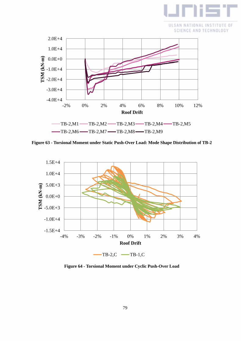
79

Figure 63 - Torsional Moment under Static Push-Over Load: Mode Shape Distribution of TB-2

Figure 64 - Torsional Moment under Cyclic Push-Over Load

-4.0E+4

-3.0E+4

-2.0E+4

-1.0E+4

0.0E+0

1.0E+4

2.0E+4

-2% 0% 2% 4% 6% 8% 10% 12%

TS

M (

kN

-m)

Roof Drift

TB-2,M1 TB-2,M2 TB-2,M3 TB-2,M4 TB-2,M5

TB-2,M6 TB-2,M7 TB-2,M8 TB-2,M9

-1.5E+4

-1.0E+4

-5.0E+3

0.0E+0

5.0E+3

1.0E+4

1.5E+4

-4% -3% -2% -1% 0% 1% 2% 3% 4%

TS

M (

kN

-m)

Roof Drift

TB-2,C TB-1,C

80

5.3.2.4 Details of Failure Process

The failure process of TB-1 and TB-2 can be examined through the local behavior that could be

measured by rotation gages at the beam hinges and axial strain gage at the tips of the wall elements.

Generally, the seismic behavior of structures can be described by the cyclic push-over load case rather

than push-over load case, because this can represent the stiffness degradation and strength

deterioration. These behavior properties can cause the reduction of deformation capacity under

earthquake loading. In this section, the results under the cyclic load case will be shown. The rotation

gage can show that which beam elements reach to the yielding point (Y), the strength reduction point

(R), or the maximum deformation point (X) during each target drift level. The axial stain gage at the

walls can measure the ultimate strength level (U), the strength reduction point (R), or the maximum

deformation point (x) for the concrete or HPFRCCs in compression, and the yielding point of

reinforcement (Y) in tension.

The local behavior of coupling beams in TB-1 was tabulated in Table 23. Here, the numbers

following the CB1 and hyphen mean the adjoining wall element around the beams. Because there are

two beams at the end of CW1, R is added to the coupling beams in the right of CW1 and L is added to

the left coupling beams with reference to Figure 33. Because the cycling loading was repeated twice

before 1.5% roof drift, the table shows repeated roof drifts with the number. The table indicates the

target roof drift when each beam element reached the points Y, R, and X. When the target roof drift

were 0.75% in positive and negative direction, the first yield rotation was measured at CB1-1R, CB1-

1L and CB1-2 in upper stories. The yielding of coupling beams gradually spread to the beams in

lower stories. At the same time, the partial CB1-1L hinges began to reach maximum rotation during -

0.75% drift. Because the first floor walls that have large thickness and a large amount of

reinforcement are considerable stiff than second floor, the weak story was occurred at these 2nd

floor

and the 1st floor beams behaved at the elastic range.

Table 24 shows the results measured from the rotation gages of coupling beams in TB-2. The

initial yield of coupling beams also occurred at 0.75% drift. This yield was not indicated at the 56th

floor, and the lower floor walls reached the Y point at the later drift level as different with TB-1. In

addition to this, CB-1-1R in lower floors of TB-2 did not yield. The hinge rotation of beam elements

reached the DR and DX point after the target drift was -1.25%. Any CB1-2 did not attain the

maximum deformation as well as CB1-1R in lower floors. The beam elements well modeled the

ductile behavior by using of HPFRCCs.

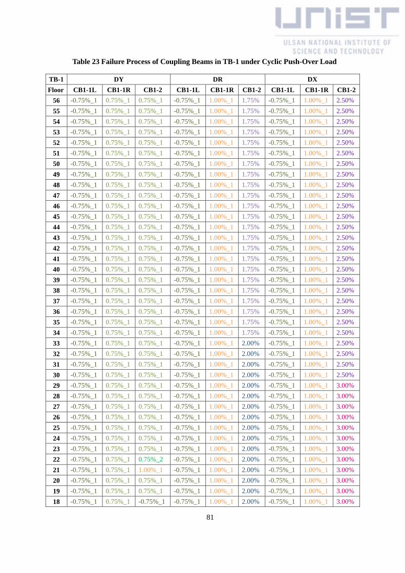
81

Table 23 Failure Process of Coupling Beams in TB-1 under Cyclic Push-Over Load

TB-1 DY DR DX

Floor CB1-1L CB1-1R CB1-2 CB1-1L CB1-1R CB1-2 CB1-1L CB1-1R CB1-2

56 -0.75%_1 0.75%_1 0.75%_1 -0.75%_1 1.00%_1 1.75% -0.75%_1 1.00%_1 2.50%

55 -0.75%_1 0.75%_1 0.75%_1 -0.75%_1 1.00%_1 1.75% -0.75%_1 1.00%_1 2.50%

54 -0.75%_1 0.75%_1 0.75%_1 -0.75%_1 1.00%_1 1.75% -0.75%_1 1.00%_1 2.50%

53 -0.75%_1 0.75%_1 0.75%_1 -0.75%_1 1.00%_1 1.75% -0.75%_1 1.00%_1 2.50%

52 -0.75%_1 0.75%_1 0.75%_1 -0.75%_1 1.00%_1 1.75% -0.75%_1 1.00%_1 2.50%

51 -0.75%_1 0.75%_1 0.75%_1 -0.75%_1 1.00%_1 1.75% -0.75%_1 1.00%_1 2.50%

50 -0.75%_1 0.75%_1 0.75%_1 -0.75%_1 1.00%_1 1.75% -0.75%_1 1.00%_1 2.50%

49 -0.75%_1 0.75%_1 0.75%_1 -0.75%_1 1.00%_1 1.75% -0.75%_1 1.00%_1 2.50%

48 -0.75%_1 0.75%_1 0.75%_1 -0.75%_1 1.00%_1 1.75% -0.75%_1 1.00%_1 2.50%

47 -0.75%_1 0.75%_1 0.75%_1 -0.75%_1 1.00%_1 1.75% -0.75%_1 1.00%_1 2.50%

46 -0.75%_1 0.75%_1 0.75%_1 -0.75%_1 1.00%_1 1.75% -0.75%_1 1.00%_1 2.50%

45 -0.75%_1 0.75%_1 0.75%_1 -0.75%_1 1.00%_1 1.75% -0.75%_1 1.00%_1 2.50%

44 -0.75%_1 0.75%_1 0.75%_1 -0.75%_1 1.00%_1 1.75% -0.75%_1 1.00%_1 2.50%

43 -0.75%_1 0.75%_1 0.75%_1 -0.75%_1 1.00%_1 1.75% -0.75%_1 1.00%_1 2.50%

42 -0.75%_1 0.75%_1 0.75%_1 -0.75%_1 1.00%_1 1.75% -0.75%_1 1.00%_1 2.50%

41 -0.75%_1 0.75%_1 0.75%_1 -0.75%_1 1.00%_1 1.75% -0.75%_1 1.00%_1 2.50%

40 -0.75%_1 0.75%_1 0.75%_1 -0.75%_1 1.00%_1 1.75% -0.75%_1 1.00%_1 2.50%

39 -0.75%_1 0.75%_1 0.75%_1 -0.75%_1 1.00%_1 1.75% -0.75%_1 1.00%_1 2.50%

38 -0.75%_1 0.75%_1 0.75%_1 -0.75%_1 1.00%_1 1.75% -0.75%_1 1.00%_1 2.50%

37 -0.75%_1 0.75%_1 0.75%_1 -0.75%_1 1.00%_1 1.75% -0.75%_1 1.00%_1 2.50%

36 -0.75%_1 0.75%_1 0.75%_1 -0.75%_1 1.00%_1 1.75% -0.75%_1 1.00%_1 2.50%

35 -0.75%_1 0.75%_1 0.75%_1 -0.75%_1 1.00%_1 1.75% -0.75%_1 1.00%_1 2.50%

34 -0.75%_1 0.75%_1 0.75%_1 -0.75%_1 1.00%_1 1.75% -0.75%_1 1.00%_1 2.50%

33 -0.75%_1 0.75%_1 0.75%_1 -0.75%_1 1.00%_1 2.00% -0.75%_1 1.00%_1 2.50%

32 -0.75%_1 0.75%_1 0.75%_1 -0.75%_1 1.00%_1 2.00% -0.75%_1 1.00%_1 2.50%

31 -0.75%_1 0.75%_1 0.75%_1 -0.75%_1 1.00%_1 2.00% -0.75%_1 1.00%_1 2.50%

30 -0.75%_1 0.75%_1 0.75%_1 -0.75%_1 1.00%_1 2.00% -0.75%_1 1.00%_1 2.50%

29 -0.75%_1 0.75%_1 0.75%_1 -0.75%_1 1.00%_1 2.00% -0.75%_1 1.00%_1 3.00%

28 -0.75%_1 0.75%_1 0.75%_1 -0.75%_1 1.00%_1 2.00% -0.75%_1 1.00%_1 3.00%

27 -0.75%_1 0.75%_1 0.75%_1 -0.75%_1 1.00%_1 2.00% -0.75%_1 1.00%_1 3.00%

26 -0.75%_1 0.75%_1 0.75%_1 -0.75%_1 1.00%_1 2.00% -0.75%_1 1.00%_1 3.00%

25 -0.75%_1 0.75%_1 0.75%_1 -0.75%_1 1.00%_1 2.00% -0.75%_1 1.00%_1 3.00%

24 -0.75%_1 0.75%_1 0.75%_1 -0.75%_1 1.00%_1 2.00% -0.75%_1 1.00%_1 3.00%

23 -0.75%_1 0.75%_1 0.75%_1 -0.75%_1 1.00%_1 2.00% -0.75%_1 1.00%_1 3.00%

22 -0.75%_1 0.75%_1 0.75%_2 -0.75%_1 1.00%_1 2.00% -0.75%_1 1.00%_1 3.00%

21 -0.75%_1 0.75%_1 1.00%_1 -0.75%_1 1.00%_1 2.00% -0.75%_1 1.00%_1 3.00%

20 -0.75%_1 0.75%_1 0.75%_1 -0.75%_1 1.00%_1 2.00% -0.75%_1 1.00%_1 3.00%

19 -0.75%_1 0.75%_1 0.75%_1 -0.75%_1 1.00%_1 2.00% -0.75%_1 1.00%_1 3.00%

18 -0.75%_1 0.75%_1 -0.75%_1 -0.75%_1 1.00%_1 2.00% -0.75%_1 1.00%_1 3.00%

82

17_1 -0.75%_1 0.75%_1 0.75%_2 -0.75%_1 1.00%_1 2.00% -1.00%_1 1.00%_1 3.00%

17 -0.75%_1 0.75%_1 1.25%_1 -0.75%_1 1.00%_1 2.00% -1.00%_1 1.00%_1 3.00%

16 -0.75%_1 0.75%_1 1.25%_1 -0.75%_1 1.00%_1 2.50% -1.00%_1 1.00%_2 3.00%

15 -0.75%_1 0.75%_1 1.25%_1 -0.75%_1 1.00%_1 2.50% -1.00%_1 1.25%_1 3.00%

14 -0.75%_1 0.75%_1 1.25%_1 -1.00%_1 1.00%_1 2.50% -1.00%_1 1.25%_1 3.00%

13 -0.75%_1 1.00%_1 1.25%_1 -1.00%_1 1.00%_2 2.50% -1.00%_1 1.25%_1 3.00%

12 -0.75%_1 1.00%_1 -1.25%_1 -1.00%_1 1.00%_2 2.50% -1.00%_1 1.25%_1 3.00%

11 -0.75%_1 1.00%_1 -1.25%_1 -1.00%_1 1.25%_1 2.50% -1.00%_1 1.25%_2 3.00%

10 -0.75%_1 1.00%_1 -1.25%_1 -1.00%_1 1.25%_1 2.50% -1.25%_1 1.50% 3.00%

9 -0.75%_1 1.00%_1 -1.25%_1 -1.00%_1 1.25%_1 2.50% -1.25%_1 1.50% 3.00%

8 -0.75%_1 1.00%_1 -1.25%_1 -1.00%_1 1.50% 2.50% -1.25%_1 1.50% 3.00%

7 -0.75%_1 1.00%_1 -1.25%_1 -1.25%_1 1.50% 2.50% -1.25%_1 1.50% 3.00%

6 -0.75%_1 1.00%_1 -1.25%_1 -1.25%_1 1.50% 2.50% -1.25%_1 1.50% 3.00%

5 -1.00%_1 1.00%_2 -1.25%_1 -1.25%_1 1.50% 2.50% -1.25%_1 1.75% -

4 -1.00%_1 1.25%_1 -1.50% -1.25%_1 1.75% 3.00% -1.25%_1 1.75% -

3 -1.00%_1 1.50% -1.50% -1.25%_1 3.00% 3.50% -1.25%_1 3.00% -

2 -1.25%_1 3.00% -1.50% -1.25%_1 3.00% 3.50% -1.25%_1 3.00% -

1 - - - - - - - - -

Table 24 Failure Process of Coupling Beams in TB-2 under Cyclic Push-Over Load

TB-2 DY DR DX

Floor CB1-1L CB1-1R CB1-2 CB1-1L CB1-1R CB1-2 CB1-1L CB1-1R CB1-2

56 -1.00%_1 1.00%_1 0.75%_1 -1.25%_1 1.50% -3.00% -1.25%_1 1.50% -

55 -0.75%_1 0.75%_2 0.75%_1 -1.25%_1 1.50% -3.00% -1.25%_1 1.50% -

54 -0.75%_1 0.75%_2 0.75%_1 -1.25%_1 1.50% -3.00% -1.25%_1 1.50% -

53 -0.75%_1 0.75%_2 0.75%_1 -1.25%_1 1.50% -3.00% -1.25%_1 1.50% -

52 -0.75%_1 0.75%_2 0.75%_1 -1.25%_1 1.50% -3.00% -1.25%_1 1.50% -

51 -0.75%_1 0.75%_2 0.75%_1 -1.25%_1 1.50% -3.00% -1.25%_1 1.50% -

50 -0.75%_1 0.75%_2 0.75%_1 -1.25%_1 1.50% -3.00% -1.25%_1 1.50% -

49 -0.75%_1 0.75%_2 0.75%_1 -1.25%_1 1.50% -3.00% -1.25%_1 1.50% -

48 -0.75%_1 0.75%_2 0.75%_1 -1.25%_1 1.50% -3.00% -1.25%_1 1.50% -

47 -0.75%_1 0.75%_1 0.75%_1 -1.25%_1 1.50% -3.00% -1.25%_1 1.50% -

46 -0.75%_1 0.75%_1 0.75%_1 -1.25%_1 1.50% -3.00% -1.25%_1 1.50% -

45 -0.75%_1 0.75%_1 0.75%_1 -1.25%_1 1.50% -3.00% -1.25%_1 1.50% -

44 -0.75%_1 0.75%_1 0.75%_1 -1.25%_1 1.50% -3.00% -1.25%_1 1.50% -

43 -0.75%_1 0.75%_1 0.75%_1 -1.25%_1 1.50% -3.00% -1.25%_1 1.50% -

42 -0.75%_1 0.75%_1 0.75%_1 -1.25%_1 1.50% -3.00% -1.25%_1 1.50% -

41 -0.75%_1 0.75%_1 0.75%_1 -1.25%_1 1.50% -3.00% -1.25%_1 1.50% -

40 -0.75%_1 0.75%_2 0.75%_1 -1.25%_1 1.50% -3.00% -1.25%_1 1.50% -

39 -0.75%_1 0.75%_2 0.75%_1 -1.25%_1 1.50% -3.00% -1.25%_1 1.50% -

38 -0.75%_1 0.75%_2 0.75%_1 -1.25%_1 1.50% -3.00% -1.25%_1 1.50% -

37 -0.75%_1 0.75%_2 0.75%_1 -1.25%_1 1.50% -3.00% -1.25%_1 1.50% -

83

36 -0.75%_1 0.75%_1 0.75%_1 -1.25%_1 1.50% -3.00% -1.25%_1 1.50% -

35 -0.75%_1 0.75%_1 0.75%_1 -1.25%_1 1.50% -3.00% -1.25%_1 1.50% -

34 -0.75%_1 0.75%_1 0.75%_1 -1.25%_1 1.50% -3.00% -1.25%_1 1.50% -

33 -0.75%_1 0.75%_1 0.75%_2 -1.25%_1 1.50% -3.00% -1.25%_1 1.50% -

32 -0.75%_1 0.75%_1 0.75%_2 -1.25%_1 1.50% -3.00% -1.25%_1 1.50% -

31 -0.75%_1 0.75%_1 0.75%_2 -1.25%_1 1.50% -3.00% -1.25%_1 1.50% -

30 -0.75%_1 0.75%_1 1.00%_1 -1.25%_1 1.50% -3.00% -1.25%_1 1.50% -

29 -0.75%_1 0.75%_1 1.00%_1 -1.25%_1 1.50% -3.00% -1.25%_2 1.50% -

28 -0.75%_1 0.75%_1 1.00%_1 -1.25%_1 1.50% -3.00% -1.25%_2 1.50% -

27 -0.75%_1 0.75%_1 1.00%_1 -1.25%_1 1.50% -3.00% -1.50% 1.50% -

26 -0.75%_1 0.75%_1 1.00%_1 -1.25%_1 1.50% -3.00% -1.50% 1.50% -

25 -0.75%_1 0.75%_1 1.00%_1 -1.25%_1 1.50% -3.00% -1.50% 1.75% -

24 -0.75%_1 0.75%_1 1.00%_1 -1.25%_1 1.50% -3.00% -1.50% 1.75% -

23 -0.75%_1 0.75%_1 1.00%_1 -1.25%_1 1.50% -3.00% -1.50% 1.75% -

22 -0.75%_1 0.75%_1 1.00%_1 -1.25%_1 1.50% -3.00% -1.50% 1.75% -

21 -0.75%_1 0.75%_1 1.00%_1 -1.25%_1 1.50% -3.00% -1.50% 1.75% -

20 -0.75%_1 0.75%_1 1.00%_1 -1.25%_1 1.50% -3.00% -1.50% 1.75% -

19 -0.75%_1 0.75%_1 1.00%_1 -1.25%_1 1.50% -3.00% -1.50% 1.75% -

18 -0.75%_1 0.75%_2 1.00%_1 -1.25%_1 1.50% -3.00% -1.50% 1.75% -

17_1 -0.75%_1 1.00%_1 1.25%_1 -1.25%_1 1.50% -3.00% -1.75% 1.75% -

17 -0.75%_1 1.00%_1 1.25%_1 -1.50% 1.50% -3.00% -1.75% 1.75% -

16 -0.75%_1 1.00%_1 1.25%_1 -1.50% 1.50% -3.00% -1.75% 1.75% -

15 -0.75%_1 1.00%_1 1.25%_1 -1.50% 1.75% -3.00% -1.75% 2.00% -

14 -1.00%_1 1.25%_1 -1.75% -1.50% - - -1.75% - -

13 -1.00%_1 1.25%_1 -1.75% -1.75% - - -1.75% - -

12 -1.00%_1 1.25%_1 -1.75% -1.75% - - -1.75% - -

11 -1.00%_1 - -1.75% -1.75% - - -1.75% - -

10 -1.00%_1 - -1.75% -1.75% - - -1.75% - -

9 -1.00%_1 - -1.75% -1.75% - - -1.75% - -

8 -1.00%_1 - -1.75% -1.75% - - -1.75% - -

7 -1.00%_1 - -1.75% -1.75% - - -2.00% - -

6 -1.25%_1 - -1.75% -1.75% - - -2.00% - -

5 -1.25%_1 - -2.00% -1.75% - - -2.00% - -

4 -1.25%_1 - -2.00% -1.75% - - -2.00% - -

3 -1.50% - -2.00% -1.75% - - -2.00% - -

2 -1.75% - -2.00% -1.75% - - -2.00% - -

1 - - - - - - - - -

84

Figure 65 describes the location and name of each strain gages at each node. The gage takes its

name from the combination of each wall element and the direction of the location. The local behavior

of the wall elements in TB-1 and TB-2 are shown in Table 25 and Table 26, respectively.

TB-1 model measured the first axial yield strain at 4th ~ 6

th floors of the left ends of CW6 during

the 1% drift, while this occurred earlier at 15th floor when 0.5% target drift in TB-2 model. The most

tensile yield in TB-1 was developed at lower stories around the 2nd

~ 5th floors, TB-2 showed the

earlier yield at around 15th floor that begin to use normal concrete after HPFRCCs. In spite of the

ductile properties of HPFRCCs, the overall behavior was worse in TB-2 by the shift of weak story. In

case of the compression, the initial behavior of TB-2 models was not significantly different with TB-1

up to -1% drift cycle. However, from 1.25% target roof drift, the compression strain gages at the

lower stories around 2nd

floor reached the DU, DR, and DX point in TB-1, while these were mainly

happen at around 15th floor of TB-2 model. The failure of TB-1 wall systems was significantly

influenced by the fracture of CW3, CW3A, CW1, and CW1A at 2nd

floor after fractures of CW6 and

CW6A. The failure of TB-2 began from fracture of CW6A at 15th floor, and this was propagated to

CW4, CW4A, and the right side of CW1and CW1A in 15th floor. And then, while the fracture was

occurred at the left side of CW1A, CW3, and CW6 in 15th floor when -3.0% drift, the structure finally

collapsed with H2 direction at this weak stories.

In case of TB-1, the initial nonlinear behavior was occurred at the coupling beam, and then the

strain gages in wall elements reached the yielding of reinforcements and ultimate strength point of

concretes. If the coupling beams failed, each shear wall is subjected to larger force than before. After

all CB1-1L and a large part of CB1-1R were failed at -1.25% roof drift, the reinforcement in 2nd

floor

of CW1 and CW1AR yielded in tension and concrete at same floor of CW1 began to reach the

ultimate strength level in compression.

The initial yielding was occurred at CW6W in TB-2 before the beams reached any yield point.

And then, the yielding of wall and beam elements was measured around the same drift cycles. After

the fails of CB1-1L and CB1-1R during -1.75% and -2.00% drift, the reinforcement was yielded and

concrete reached at the DR point in second floor of CW1 and CW1A. Generally, the previous

experiments for coupled walls demonstrate that ductile coupling beams improve some performances

of the coupled wall system such as the ductility or energy dissipation. In spite of more ductile

behavior of the coupling beams than that of TB-1, the performance of TB-2 was worsened due to the

early development of a weak story.

85

Figure 65 - Location of Strain Gages for Tall Building

Table 25 Failure Process of Walls in TB-1 under Cyclic Push-Over Load

Tension Strain Compression Strain

DY DU DR

Roof Drift Element Floor Roof

Drift Element Floor Roof Drift Element Floor

1.00%_1 CW6W 4~6F 0.75%_1 CW6AE 2F -1.25%_1 CW6W 2F

1.00%_2 CW6W 7~13F -0.75%_1 CW6W 2~5F 1.50% CW6AE 4F

-1.00%_2 CW6AE 4~7F 1.00%_1

CW6AE 2,4,11F -1.50% CW1W 2F

1.25%_1 CW6W 2,14~17F CW6AE 5F

-2.50%

CW2LW 2F

-1.25%_1

CW1ARE 2F -1.00%_1 CW6W 6,7,11F CW3 2F

CW1ALE 2F

1.25%_1 CW6AE

6~10F,

12~14F

CW3A 2F

CW1E 2F CW6E 2F

CW2RE 2F CW6AE 15F 3.00% CW1ALE 2F

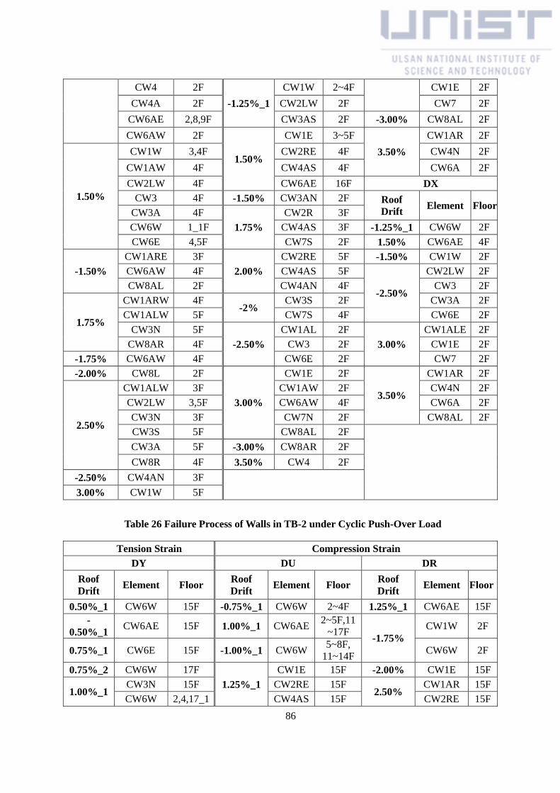
86

CW4 2F

-1.25%_1

CW1W 2~4F CW1E 2F

CW4A 2F CW2LW 2F CW7 2F

CW6AE 2,8,9F CW3AS 2F -3.00% CW8AL 2F

CW6AW 2F

1.50%

CW1E 3~5F

3.50%

CW1AR 2F

1.50%

CW1W 3,4F CW2RE 4F CW4N 2F

CW1AW 4F CW4AS 4F CW6A 2F

CW2LW 4F CW6AE 16F DX

CW3 4F -1.50% CW3AN 2F Roof

Drift Element Floor

CW3A 4F

1.75%

CW2R 3F

CW6W 1_1F CW4AS 3F -1.25%_1 CW6W 2F

CW6E 4,5F CW7S 2F 1.50% CW6AE 4F

-1.50%

CW1ARE 3F

2.00%

CW2RE 5F -1.50% CW1W 2F

CW6AW 4F CW4AS 5F

-2.50%

CW2LW 2F

CW8AL 2F CW4AN 4F CW3 2F

1.75%

CW1ARW 4F -2%

CW3S 2F CW3A 2F

CW1ALW 5F CW7S 4F CW6E 2F

CW3N 5F

-2.50%

CW1AL 2F

3.00%

CW1ALE 2F

CW8AR 4F CW3 2F CW1E 2F

-1.75% CW6AW 4F CW6E 2F CW7 2F

-2.00% CW8L 2F

3.00%

CW1E 2F

3.50%

CW1AR 2F

2.50%

CW1ALW 3F CW1AW 2F CW4N 2F

CW2LW 3,5F CW6AW 4F CW6A 2F

CW3N 3F CW7N 2F CW8AL 2F

CW3S 5F CW8AL 2F

CW3A 5F -3.00% CW8AR 2F

CW8R 4F 3.50% CW4 2F

-2.50% CW4AN 3F

3.00% CW1W 5F

Table 26 Failure Process of Walls in TB-2 under Cyclic Push-Over Load

Tension Strain Compression Strain

DY DU DR

Roof

Drift Element Floor

Roof

Drift Element Floor

Roof

Drift Element Floor

0.50%_1 CW6W 15F -0.75%_1 CW6W 2~4F 1.25%_1 CW6AE 15F

-

0.50%_1 CW6AE 15F 1.00%_1 CW6AE

2~5F,11

~17F -1.75%

CW1W 2F

0.75%_1 CW6E 15F -1.00%_1 CW6W 5~8F,

11~14F CW6W 2F

0.75%_2 CW6W 17F

1.25%_1

CW1E 15F -2.00% CW1E 15F

1.00%_1 CW3N 15F CW2RE 15F

2.50% CW1AR 15F

CW6W 2,4,17_1 CW4AS 15F CW2RE 15F

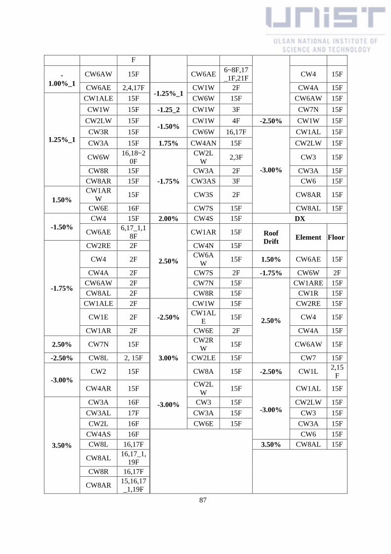
87

F

-

1.00%_1

CW6AW 15F CW6AE 6~8F,17

_1F,21F CW4 15F

CW6AE 2,4,17F -1.25%_1

CW1W 2F CW4A 15F

1.25%_1

CW1ALE 15F CW6W 15F CW6AW 15F

CW1W 15F -1.25_2 CW1W 3F CW7N 15F

CW2LW 15F -1.50%

CW1W 4F -2.50% CW1W 15F

CW3R 15F CW6W 16,17F

-3.00%

CW1AL 15F

CW3A 15F 1.75% CW4AN 15F CW2LW 15F

CW6W 16,18~2

0F

-1.75%

CW2L

W 2,3F CW3 15F

CW8R 15F CW3A 2F CW3A 15F

CW8AR 15F CW3AS 3F CW6 15F

1.50%

CW1AR

W 15F CW3S 2F CW8AR 15F

CW6E 16F CW7S 15F CW8AL 15F

-1.50%

CW4 15F 2.00% CW4S 15F DX

CW6AE 6,17_1,1

8F

2.50%

CW1AR 15F Roof

Drift Element Floor

-1.75%

CW2RE 2F CW4N 15F

CW4 2F CW6A

W 15F 1.50% CW6AE 15F

CW4A 2F CW7S 2F -1.75% CW6W 2F

CW6AW 2F CW7N 15F

2.50%

CW1ARE 15F

CW8AL 2F CW8R 15F CW1R 15F

CW1ALE 2F

-2.50%

CW1W 15F CW2RE 15F

CW1E 2F CW1AL

E 15F CW4 15F

CW1AR 2F CW6E 2F CW4A 15F

2.50% CW7N 15F

3.00%

CW2R

W 15F CW6AW 15F

-2.50% CW8L 2, 15F CW2LE 15F CW7 15F

-3.00%

CW2 15F CW8A 15F -2.50% CW1L 2,15

F

CW4AR 15F

-3.00%

CW2L

W 15F

-3.00%

CW1AL 15F

3.50%

CW3A 16F CW3 15F CW2LW 15F

CW3AL 17F CW3A 15F CW3 15F

CW2L 16F CW6E 15F CW3A 15F

CW4AS 16F

CW6 15F

CW8L 16,17F 3.50% CW8AL 15F

CW8AL 16,17_1,

19F

CW8R 16,17F

CW8AR 15,16,17

_1,19F

88

DX

Roof

Drift Element Floor

1.75% CW6W 15F

-2.00% CW6AE 2F

2.50%

CW2LW 15F

CW3A 15F

CW3S 15F

CW6E 15F

-3.00% CW8L 15F

3.50% CW8R 15F

89

5.3.3 Earthquake Load

5.3.3.1 Story Drift

Figure 66 shows the interstory drift of TB-1 and TB-2 subjected to El Centro earthquake loads

when each model has a maximum base shear. The interstory drift indicates the relative floor

displacement divided by the floor height. The story drift of TB-2 has almost same results with the

story drift of TB-1. Most of story drift occurred at lower part. The largest story drift is about 0.26% at

12th floor, and this value is remarkably small.

Figure 66 - Story Drift under an Earthquake Load at Instant of Maximum Base Shear

5.3.3.2 Base Shear

Figure 67 demonstrates the time histories of base shear in H1 direction for TB-1 and TB-2, and

both models have similar results. For this earthquake load, the maximum base shear is about 45,000

kN in both models. At the instant of this maximum base shear, story by story lateral forces for TB-1

and TB-2 are shown in Figure 68 and the lateral forces are concentrated on the lower part. By the

strain gage, TB-1 and TB-2 under this earthquake load have linear behaviors results in spite of the

relatively large base shear compared with cyclic push-over load cases. These cyclic loads had a

vertical distribution with Cvx factor and this distribution case was similar with the first three mode

distribution cases. Therefore, the response of these structures follows higher modes and has a linear

0

10

20

30

40

50

60

-0.1% 0.0% 0.1% 0.2% 0.3%

Flo

or

Story Drift

TB-1,H1

TB-1,H2

TB-2,H1

TB-2,H2

90

behavior under the El Centro earthquake. As a result, the use of HPFRCC did not have a significant

impact on the behavior of the structures.

Figure 67 - Base Shear under an Earthquake Load

Figure 68 – Story by Story Lateral Force under an Earthquake Load at Instant of Maximum

Base Shear

-6.0E+4

-4.0E+4

-2.0E+4

0.0E+0

2.0E+4

4.0E+4

6.0E+4

0 5 10 15 20 25 30 35

Ba

se S

hea

r (k

N)

Time (s)

TB-2 TB-1

0

10

20

30

40

50

60

-2000 0 2000 4000

Flo

or

Story-by-story lateral force (kN)

TB-2,H1,MaxBS

TB-1,H1,MaxBS

91

5.3.3.3 Base Moment

Figure 69 represents hysteretic curves about the overturning moment of TB-1 and TB-2 under the

El Centro earthquake loads. The two models have similar results, and the largest moment is about

2,500,000kN-m. This value is relatively smaller than the results from cyclic push-over load case.

However, the maximum torsional moments of TB-1 and TB-2 are sustainably larger than that of cyclic

push-over load case (Figure 70). For this ground motion, the structures have elastic behavior despite

the large torsional moments.

Figure 69 - Overturning Moment under an Earthquake Load

Figure 70 - Torsional Moment under an Earthquake Load

-3.0E+6

-2.0E+6

-1.0E+6

0.0E+0

1.0E+6

2.0E+6

3.0E+6

0 5 10 15 20 25 30 35

OT

M (

kN

-m)

Time (s)

TB-2,R5%_9 TB-1,R5%_9

-3.0E+5

-2.0E+5

-1.0E+5

0.0E+0

1.0E+5

2.0E+5

3.0E+5

0 5 10 15 20 25 30 35

TS

M (

kN

-m)

Time (s)

TB-2,R5%_9 TB-1,R5%_9

92

Chapter 6. Conclusions

The main property of high performance fiber-reinforced cement composites (HPFRCCs) is

characterized by the strain hardening behavior, and the enhanced response can be generally expected

with the structure using this material compared to the normal concrete structure. This study is to

investigate the seismic performance of a tall building with coupled wall systems using HPFRCCs. For

this purpose, the first work is the development of analysis methods for the coupled wall systems based

on the previously proposed methods to represent the nonlinear behavior of each component. The more

reliable and economical modeling methods for coupling beams and shear walls was considered. The

behavior of coupling beams was described with Moment Hinge Model including the reinforcement

slip effect, and Fiber Model was selected for the wall modeling.

Two 4-story coupled wall specimens (CW-1 and CW-2) which were tested by Lequesne (2011)

were used to check a reliability of the proposed modeling methods. Both specimens had the

HPFRCCs coupling beams, and the walls of CW-1 followed a traditional RC design while the 1st floor

wall of CW-2 used HPFRCCs materials with reduced reinforcement. The test results about

overturning moment were compared with the analysis results to verify the overall behavior of the

specimens under the reversed cyclic loading. The measured yielding process was also discussed for

the comparison of the local behavior. The overall behavior of the tested couple wall systems was well

simulated by the proposed modeling methods, especially such as the initial strength, stiffness, and

energy dissipation. In case of the local behavior model, the location and time of the yielding

occurrence almost corresponded with the test results. The analysis also well represents the strength

increases observed in the measured strength of CW-2 by using HPFRCCs in comparison with CW-1.

On the other hand, the models could not simulate the sliding shear displacement of coupling beam in

CW-1 at 2% wall drift and shear fail of the wall in CW-2 at -2.5% wall drift.

These modeling methods for coupled wall system were applied with a 56-story tall building

model (TB-1 and TB-2) to observe the effectiveness of HPFRCCs in coupling beams and walls 1/4

height of the building. The main analysis results with different conditions are summarized as follows:

The constant gravity loads were applied considering the weight of the structure, assumed

super imposed dead loads, and live loads. When the tall building was subjected to the

static push-over loads with this gravity loads, the structure system had substantially larger

base shear strength and strength reductions than the results without gravity loads. The

differentials of the strength between two cases were even higher than P-Δ shear.

Various types of the vertical distribution of lateral loads were modeled in this study. The

result of the model with uniform distribution showed the largest base shear forces than the

93

triangular and Cvx factor distribution cases. However, they had a similar maximum

overturning moment results. In case of TB-2, the model with Cvx factor distribution had a

different interstory drift result that described a shift of weak story at the last wall drift.

The results from lateral loads with modal distributions indicated that the first three mode

cases had a similar result with the results from Cvx factor distribution case. The higher

mode cases showed the larger base shear results and the smaller overturning moment

results.

The buildings under the reversed cyclic loading represented the large strength degradation

at the latter cycles which is important properties of reinforced concrete members to

account for the cumulated damage.

The HPFRCCs coupling beams used in TB-2 showed more ductile behavior than the

normal concrete coupling beams in TB-1.

Failure processes of TB-1 and TB-2 were very different each other. The initial nonlinear

behavior of TB-1 was dominated by the yielding of coupling beams, while the nonlinear

behavior of walls in TB-2 at the weak story caused the initial response.

The use HPFRCCs in all beams and the lower 1/4 stories (1~14F) of walls of TB-2 leaded

to the earlier occurrence of weak story at 15th floor.

For El Centro earthquake load cases, TB-1 and TB-2 had elastic behavior in spite of the

large base shear. This response could be caused by the higher mode effects.

This study provides the information about the nonlinear analysis of tall coupled wall systems

using HPFRCCs without design changes of the structure. When the better performance and

construction work are intended due to the advantage of HPFRCCs material, the proper design changes

are required in the HPFRCC walls such as the reduction of reinforcement quantity to prevent the

occurrence of weak story in the higher floors before the HPFRCC coupling beams dissipate the

sufficient energy.

References

1. ACI Committee 318 (2008), Building Code Requirements for Structural Concrete (ACI 318-

08), American Concrete Institute, Farmington Hills, MI.

2. Aristizabal-Ochoa, J. D. (1983). Seismic analysis of slender coupled walls. Journal of

Structural Engineering, ASCE 109(7), 1538-1552.

3. Aristizabal-Ochoa, J. D., & Sozen, M. A. (1976). Behavior of ten-story reinforced concrete

walls subjected to earthquake motions. Doctoral dissertation, University of Illinois, Urbana-

Champaign, IL.

4. ASCE/SEI 41/06, 2007, Seismic Rehabilitation of Existing Buildings, American Society of

Civil Engineers, Reston, Virginia.

5. Barney, G. B. (1980). Behavior of coupling beams under load reversals. Portland Cement

Association.

6. Canbolat, B. A., Parra-Montesinos, G. J., & Wight, J. K. (2005). Experimental study on

seismic behavior of high-performance fiber-reinforced cement composite coupling beams. ACI

Structural Journal, 102(1).

7. Canbolat, B. A., Parra-Montesinos, G. J., & Wight, J. K. (2005). Experimental study on

seismic behavior of high-performance fiber-reinforced cement composite coupling beams. ACI

Structural Journal, 102(1).

8. Chang, G. A., & Mander, J. B. (1994). Seismic energy based fatigue damage analysis of bridge

columns: part 1-evaluation of seismic capacity.

9. Cho, Y. M., Seo, S. Y., & Yoon, S. J. (2007). Nonlinear Behavior Characteristic of Reinforced

Concrete Shear Wall. Architectural Institute of Korea, v.01, p519-523

10. Colotti, V. (1993). Shear behavior of RC structural walls. Journal of Structural Engineering,

119(3), 728-746.

11. Computers and Structures (CSI), Inc.,. (2006). PERFORM 3D, User Guide v4, Non-linear

Analysis and Performance Assessment for 3D Structures, Berkeley, CA.

12. Computers and Structures, Inc.(CSI). (2006). PERFORM-3D: Nonlinear Analysis and

Performance Assessment for 3-D Structures: Version 4.

13. Filippou, F. C., D'Ambrisi, A., & Issa, A. (1999). Modeling of reinforcement slip in RC frame

members under cyclic excitations. ACI Structural Journal, 96(3), 327-335.

14. Galano, L., & Vignoli, A. (2000). Seismic behavior of short coupling beams with different

reinforcement layouts. ACI Structural Journal, 97(6).

15. Hisatoku, T. and Matano, H. (1972). Experimental Study on Physical Characteristics of

Coupled Shear Wall. Takenaka Gijutsu Kenkyu Hokoku (Japanese), (8), p. 1-23.

16. Hognestad, E. (1952, October). Inelastic behavior in tests of eccentrically loaded short

reinforced concrete columns. In ACI Journal Proceedings (Vol. 49, No. 10). ACI.

17. Kabeyasawa, T., Shiohara, H., Otani, S., & Aoyama, H. (1983). Analysis of the full-scale

seven-story reinforced concrete test structure. Journal of the Faculty of Engineering, 37(2),

431-478.

18. Kent, D. C., & Park, R. (1971). Flexural members with confined concrete. Journal of the

Structural Division, 97(7), 1969-1990.

19. Kwan, A. K. H., & Zhao, Z. Z. (2002). Cyclic behaviour of deep reinforced concrete coupling

beams. Proceedings of the ICE-Structures and Buildings, 152(3), 283-293.

20. Lee, J. H., jeon, Y., & Kim, J. K. (2011). Response Modification Factors of Rectangular

Staggered Wall System Buildings. Architectural Institute of Korea, v.01, p519-523

21. Lequesne, R. D. (2011). Behavior and design of high-performance fiber-reinforced concrete

coupling beams and coupled-wall systems, Doctoral dissertation, The University of Michigan.

22. Lu, X., & Chen, Y. (2005). Modeling of coupled shear walls and its experimental verification.

Journal of Structural Engineering, ASCE 131(1), 75-84.

23. Lybas, J. M., & Sozen, M. A. (1977). Effect of beam strength and stiffness on dynamic

behavior of reinforced concrete coupled walls. Doctoral dissertation, University of Illinois,

Urbana-Champaign, IL.

24. Naaman, A. E. (1996). Characterization of high performance fiber reinforced cement

composites-HPFRCC. In High performance fiber reinforced cement composites, p. 1-23.

25. Naish, D. A. B. (2010). Testing and modeling of reinforced concrete coupling beams (Vol. 71,

No. 10).

26. Naish, D., Fry, J. A., Klemencic, R., & Wallace, J. (2009). Reinforced Concrete Link Beams:

Alternative Details for Improved Constructability. Rep. to Charles Pankow Foundation.

27. Nayar, K. K., & Coull, A. (1976). Elastoplastic analysis of coupled shear walls. Journal of the

structural Division, ASCE 102(9), 1845-1860.

28. Parra-Montesinos, G. J. (2006). Shear strength of beams with deformed steel fibers.

CONCRETE INTERNATIONAL-DETROIT-, 28(11), 57.

29. Paulay, T. (1969). The coupling of shear walls, Doctoral dissertation, University of Canterbury,

Christchurch, New Zealand.

30. Paulay, T. (1971). Coupling beams of reinforced concrete shear walls. Journal of the Structural

Division, 97(3), 843-862.

31. Paulay, T., & Binney, J. R. (1974). Diagonally reinforced coupling beams of shear walls. ACI

special publication, 42.

32. Petrangeli, M., Pinto, P. E., & Ciampi, V. (1999). Fiber element for cyclic bending and shear of

RC structures. I: Theory. Journal of Engineering Mechanics, 125(9), 994-1001.

33. Santhakumar, A. R. (1974). Ductility of coupled shear walls. (Doctoral dissertation, University

of Canterbury).

34. Shahrooz, B. M., & Fortney, P. J. (2005). The next generation of coupling beams. Report no.

UC-CII, 5(01).

35. Shiu, K. N., Aristizabal-Ochoa, J. D., Barney, G. B., Fiorato, A. E., & Corley, W. G. (1981).

Earthquake resistant structural walls: Coupled wall tests. NASA STI/Recon Technical Report

N, 82, 21450.

36. Subedi, N. K. (1991). RC-coupled shear wall structures. I: analysis of coupling beams. Journal

of Structural Engineering, ASCE 117(3), 667-680.

37. Takayanagi, T., & Schnobrich, W. C. (1976). Computed behavior of reinforced concrete

coupled shear walls. Civil Engineering Studies, Structural Research Series, University of

Illinois.

38. Tassios, T. P., Moretti, M., & Bezas, A. (1996). On the behavior and ductility of reinforced

concrete coupling beams of shear walls. ACI Structural Journal, 93(6).

39. Vulcano, A., Bertero, V. V., & Colotti, V. (1988). Analytical modeling of R/C structural walls.

In 9th World Conference on Earthquake Engineering (Vol. 6, pp. 41-6).

40. Wilson, E. L., & Habibullah, A. (1995). SAP2000, Structural Analysis Programs. Computers

and Structures, Inc., University Avenue, Berkeley, California, USA.

41. Xiao, Y., Esmaeily-Ghasemabadi, A., & Wu, H. (1999). High-strength concrete short beams

subjected to cyclic shear. ACI Structural Journal, 96(3).