nonlinear adaptive observer for a lithium-ion battery s ... applications in...derived from the...

S. Dey1

Department of Automotive Engineering,

Clemson University,

4 Research Drive,

Greenville, SC 29607

e-mail: [email protected]

B. AyalewDepartment of Automotive Engineering,

Clemson University,

4 Research Drive,



P. PisuDepartment of Automotive Engineering,

Clemson University,

4 Research Drive,



Nonlinear Adaptive Observerfor a Lithium-Ion BatteryCell Based on CoupledElectrochemical–Thermal ModelReal-time estimation of battery internal states and physical parameters is of the utmostimportance for intelligent battery management systems (BMS). Electrochemical models,derived from the principles of electrochemistry, are arguably more accurate in capturingthe physical mechanism of the battery cells than their counterpart data-driven or equiva-lent circuit models (ECM). Moreover, the electrochemical phenomena inside the batterycells are coupled with the thermal dynamics of the cells. Therefore, consideration ofthe coupling between electrochemical and thermal dynamics inside the battery cellcan be potentially advantageous for improving the accuracy of the estimation. In thispaper, a nonlinear adaptive observer scheme is developed based on a coupledelectrochemical–thermal model of a Li-ion battery cell. The proposed adaptive observerscheme estimates the distributed Li-ion concentration and temperature states inside theelectrode, and some of the electrochemical model parameters, simultaneously. Thesestates and parameters determine the state of charge (SOC) and state of health (SOH) ofthe battery cell. The adaptive scheme is split into two separate but coupled observers,which simplifies the design and gain tuning procedures. The design relies on a Lyapu-nov’s stability analysis of the observers, which guarantees the convergence of the com-bined state-parameter estimates. To validate the effectiveness of the scheme, bothsimulation and experimental studies are performed. The results show that the adaptivescheme is able to estimate the desired variables with reasonable accuracy. Finally, somescenarios are described where the performance of the scheme degrades.[DOI: 10.1115/1.4030972]

Introduction

Li-ion batteries are now the leading solutions for electrifiedtransportation and stationary energy storage applications due totheir several beneficial features in high energy and power density,absence of memory effect and self-discharge, low environmentalimpact, etc. However, they still suffer from safety and reliabilityconcerns. These concerns can be addressed via the advancedBMS, which require precise knowledge of battery internal infor-mation like SOC and SOH.

The core challenge for acquiring these internal information isthat, in general, the only available information in real-time isboundary measurement of voltage, current, and temperature. Thisfact underscores the importance of reliable estimation algorithmsthat compute the internal information in the Li-ion cells fromthese limited measurements. Moreover, there are several otherchallenges in SOC and SOH estimation of Li-ion cells [1]. One ofthem arises from the spatially distributed nature of Li-ion concen-trations inside the cell. Other crucial challenges relate to paramet-ric uncertainties with aging (both with charge/discharge historyand calendar time), cell-to-cell manufacturing variability, and var-iations in Li-ion chemistry. In this paper, we address some ofthese challenges by proposing an electrochemical–thermal model-based adaptive estimation scheme for online joint estimation ofthe distributed Li-ion concentration in the electrodes, and someuncertain model parameters. In addition to improving the accu-racy of the SOC estimation, online parameter estimates can beused as SOH indicators.

In the literature, the different estimation algorithms proposedfor Li-ion batteries can be broadly classified based on the type ofmodel used: (1) data-driven model-based algorithms [2,3], (2)ECM-based algorithms [4–7], and (3) electrochemical model-based algorithms. Although data-driven approaches are simple inimplementation and design, the drawback lies in the requirementof large amount of data over the whole operating regime of thebattery and lack of physical meaning of the data-driven modelparameters. Similarly, the parameters of the ECM basedapproaches (for example, the resistors and capacitors) have to bemodeled as functions of different operating conditions such asSOC, temperature, etc., to capture the battery behavior over largeroperating range.

Electrochemical model-based approaches, developed fromporous electrode and concentrated solution theories, are moreaccurate compared to other kinds of models [8]. However, full-order electrochemical model (pseudo-two-dimensional (P2D)model) consists of coupled nonlinear partial differential equations(PDE) [9]. A few methods exist in literature that improves thecomputational efficiency of P2D model, for instance in Ref. [10],a Legendre polynomial and Galerkin projection based approach isused. However, the complex mathematical structure of P2D modelstill remains one of the difficult factors for suitable estimatordesign. This complex mathematical structure has led to differentkinds of model reductions in the literature before the estimator isdesigned. For example, a residue grouping with a linear Kalmanfilter was used in Ref. [11] and a constant electrolyte concentra-tion assumption with Luenberger observer was used in Ref. [12].In Ref. [13], a reduced-order electrochemical model is developedusing quasi-linearization and Pade approximation. Recently, aphysics-based second-order Li-ion battery model is presented inRef. [14]. Another reduced-order electrochemical model calledthe single particle model (SPM) where the electrodes are

1Corresponding author.Contributed by the Dynamic Systems Division of ASME for publication in the

JOURNAL OF DYNAMIC SYSTEMS, MEASUREMENT, AND CONTROL. Manuscript receivedDecember 17, 2014; final manuscript received June 18, 2015; published onlineAugust 13, 2015. Assoc. Editor: Junmin Wang.

Journal of Dynamic Systems, Measurement, and Control NOVEMBER 2015, Vol. 137 / 111005-1Copyright VC 2015 by ASME

Downloaded From: http://dynamicsystems.asmedigitalcollection.asme.org/ on 08/16/2015 Terms of Use: http://www.asme.org/about-asme/terms-of-use

approximated as spherical particles is also popular in SOC estima-tor designs [15–17]. The authors of the present paper proposedSPM-based nonlinear observer designs for the SOC estimation inRefs. [18,19].

Unlike the well-investigated SOC estimation problem, adaptiveSOC estimation or the simultaneous state-parameter estimationproblem is relatively less explored for electrochemical models.Some of the existing works use multirate particle filter [20],unscented Kalman filter [21], iterated extended Kalman filter[22,23] for adaptive SOC estimation. The drawback of theseapproaches lies in the difficulty to theoretically verify the conver-gence of the estimators. In another work [24], an adaptive PDEobserver and least square parameter estimator based framework ispresented for the same problem. However, stability of the com-bined state and parameter estimators was not verified analytically.In Refs. [25,26], a nonlinear geometric observer based approach ispresented for adaptive estimation of battery SOC and parameterswith theoretical verification of error convergence. However, theLi-ion diffusion dynamics and the Li-ion spatial distribution in thebattery electrode are ignored. Moreover, thermal effects are notconsidered. As will be seen later, the approach presented in pres-ent paper takes the Li-ion diffusion and spatial distribution intoconsideration along with considering the thermal effects. Theauthors of the current paper also proposed a sliding mode observerbased approach in Ref. [27] for adaptive estimation of SOC. How-ever, the drawback of the approach is that a high initial error incontact resistance estimation may lead to instability of thescheme. Other than adaptive estimation techniques, recently aSOH monitoring technique is presented that essentially monitorsthe side reaction current density of the battery via retrospectivecost-subsystem identification [28,29].

Other than SOC and SOH, battery temperature is anotherimportant quantity that is used by BMS for thermal managementof the batteries. Some recent results exist in literature for tempera-ture estimation. For example, a linear parameter varying observer-based approach is presented in Ref. [30] for temperature estima-tion of automotive battery packs. A lumped parameter thermalmodel has been presented in Ref. [31] to capture surface and coretemperature of the battery and used for adaptive observer-basedtemperature estimation along with health monitoring via internalresistance estimation [32]. Further, the work [32] is extended totemperature estimation under unknown cooling condition [33] andto parameterization and observability analysis of a battery cluster[34]. However, these approaches use ECM to capture the batteryelectrical and SOC dynamics. In Ref. [35], an enhanced SPM isused considering temperature and electrolyte effects to design aLuenberger observer for SOC estimation. However, the modelparameters were assumed to be known and parameter estimationproblem is not addressed. In this paper, we extend theseresearches by presenting an electrochemical model-based state-parameter estimation approach considering the thermal dynamicsof the battery cell.

From the above review, it can be noted that most of theelectrochemical–model based adaptive estimation approachescited above consider only electrochemical dynamics under iso-thermal conditions. However, there is a bidirectional couplingbetween the electrochemical and thermal dynamics of a Li-ioncell. In Refs. [12,36], numerical and experimental results haveshown that inclusion of the thermal model may lead to significantimprovement in the SOC estimation accuracy. This observation isalso consistent with the physical behavior of the cell which showsa bidirectional coupling captured by the coupled model as fol-lows: in electrochemical model, the open circuit potential andsome parameters are affected by temperature changes, whereas inthe thermal model, the electrochemical overpotential and open cir-cuit potential contribute to heat generation [37].

To address the above issues, we proposed a Lyapunov-basednonlinear adaptive observer design based on a combinedelectrochemical–thermal model of a Li-ion cell in Ref. [38]. Inthis paper, we extend this preliminary work by including the

following: (1) detailing the discussion on the modeling of theLi-ion cell, (2) relaxing the constant contact resistance assumptionof our previous work [38] and re-establishing the convergenceproof of the adaptive observer considering temperature depend-ence of the contact resistance, (3) adding experimental studies ona commercial Li-ion cell, and (4) including discussions on the lim-itations of the proposed observer scheme. We also provide an ana-lytical proof of convergence for the overall adaptive schemecombining state and parameter estimators. In this study, we utilizethe single particle electrochemical model (SPM) along withlumped thermal dynamics [39] to derive the adaptive observers.Three parameters, namely, diffusion coefficient, contact resist-ance, and active material volume fraction, are estimated alongwith the SOC, and may be used as SOH indicators [40].

The rest of the paper is organized as follows: The section,Lithium-Ion Cell Electrochemical-Thermal Model, discusses theelectrochemical–thermal modeling of Li-ion cell. After that theadaptive scheme is described. Next, simulation and experimentalresults are provided. Then some potential failure scenarios areillustrated for the adaptive scheme, and finally, the concludingremarks are summarized.

Lithium-Ion Cell Electrochemical–Thermal Model

The benchmark Li-ion cell electrochemical model is the P2Dmodel derived from the porous electrode and concentrated solu-tion theories [9]. It describes mass and charge conservation in thesolid active material and the electrolyte along with the electro-chemical kinetics described by Butler–Volmer equation. Althoughthere exist some approaches, e.g., [10] that improve the computa-tional efficiency of P2D model, the complex mathematical struc-ture still makes it unsuitable for real-time estimator design.Owing to this, researchers generally resort to model reductiontechniques to derive a model suitable for real-time estimatordesign. The SPM is one of the popular reduced electrochemicalmodels that we adopt in this paper.

Essentially, the SPM is derived by approximating each elec-trode as a single spherical particle and applying volume-averagingassumptions [15,16]. This approximation leads to two linear diffu-sion PDEs for Li-ion mass conservation in both electrodes givenby Eq. (1). The output voltage map is derived fromButler–Volmer kinetics, electrical potential, and electrode thermo-dynamics and is given by Eq. (2)

@c6s

@t¼ D6

s ðTÞr2

@

@rr2 @c6

s

@r

� �@c6

s

@r

��r¼0

¼ 0;@c6

s

@r

��r¼R

¼ 6I

a6s FD6

s ðTÞAL6

(1)

V ¼�RT

�aþFsinh�1 I

2aþs ALþiþ0

� ��

�RT

�a�Fsinh�1 I

2a�s AL�i�0

� �

þ Uþ cþs;e;T� �

� U� c�s;e;T� �

� Rf ðTÞI (2)

where Uþ and U� are the open-circuit potentials as functions of Li-ion surface concentration and temperature, c6

s is the Li-ion concen-tration of the positive and negative electrode, cþs;e and c�s;e are thesurface concentrations of the positive and negative electrode, V isthe output voltage, and I is the input current (the reader may refer tothe Nomenclature for the definitions of the rest of the variables).The i60 are the exchange current densities given by

i60 ¼ K6ðTÞffiffiffiffiffiffiffiffiffiffiffiffiffiffiffiffiffiffiffiffiffiffiffiffiffiffiffiffiffiffiffiffiffiffiffiffiffiffifficec6

s;e c6s;max � c6

s;e

� �r(3)

Along with the electrochemical SPM model, the followinglumped thermal model derived from the energy balance of the cellis considered [39] and is given by

111005-2 / Vol. 137, NOVEMBER 2015 Transactions of the ASME


qvCpdT

dt¼ I Uþ cþs;e;T

� ��U� c�s;e;T

� ��V� T

@Uþ

@T� @U�

@T

� �� hAsðT�T1Þ (4)

where T is the lumped averaged temperature of the cell andð@U6=@TÞ are functions of c6

s;e [39]. Here, a thermal modelingapproach in Refs. [39,41] is followed where a lumped thermalmodel is applied that predicts a lumped-temperature averagedover the cell. However, more detailed thermal model, e.g., the onein Refs. [31,32] can be applied here which may be considered as afuture extension of the present work. Now considering (4), notethat the temperature affects the open-circuit potential and overpotential terms in Eq. (2), whereas U6 and @U6=@T contribute tothe heat generation in Eq. (4). Moreover, in this study, we assumethat the solid phase diffusion coefficients (D6

s ) and the reaction rateconstants (K6) show Arrhenius dependence on temperature [39].Apart from those, the contact resistance (Rf ) is also a function oftemperature although the dependence is assumed to be linear. Tosummarize, the temperature-dependent parameters are modeled by

K6 Tð Þ ¼ K6refexp

E6K

�R

1

T� 1

Tref

� ��

D6s Tð Þ ¼ D6

s;refexpE6

Ds

�R

1

T� 1

Tref

� �� Rf Tð Þ ¼ Rf 0 þ aT

(5)

where Tref is reference temperature, K6ref and D6

s;ref are the parame-ter values at that reference temperature, Rf 0 is the constant part ofthe contact resistance and a is the proportional constant.

Remark 1. In general, the contact resistance Rf could be a non-linear function of the temperature. However, the linear depend-ence of Rf on temperature assumed here will be helpful insimplifying the observer design problem in the next section,Adaptive Observer Design.

In this study, we use the following approximation of the opencircuit potential expression [39]:

U6 c6s;e;T

� �� U6 c6

s;e;Tref

� �þ @U6

@TðT � TrefÞ (6)

Note that there are some simplifying assumptions taken whiledeveloping the SPM. First, the electrolyte dynamics is not taken intoaccount. The solid material charge dynamics is disregarded whilethe molar flux is averaged. Moreover, the SPM is more suitable forlower charge/discharge rates when the mass and charge transportthrough the electrolyte are negligible. In recent literature, someimproved versions of the SPM are presented which relax some ofthese aforementioned assumptions and extend the model to be appli-cable for higher charge/discharge scenarios. In Ref. [42], the electro-lyte concentration and potential dynamics are considered byapproximating them using polynomial functions. A similar exten-sion is developed in Ref. [43] including nonuniform reaction distri-bution. In Ref. [44], a seventh-order, enhanced SPM with electrolytediffusion and temperature-dependent parameters is developed toextend the conventional SPM. Nevertheless, despite the improvedpredictive capability of these enhanced models, we used the conven-tional SPM [15,16]; due to its suitability for the analytical adaptiveobserver designs, we propose here. In any case, it should be empha-sized that the conventional SPM is a tradeoff between amounts ofelectrochemical phenomenon captured and the simplified formneeded for observer design and real-time implementation.

Model Reduction and Finite-Dimensional

Approximation

The two-electrode SPM discussed in the previous section,Lithium-Ion Cell Electrochemical-Thermal Model, suffers from

weak observability of the full state from differential voltage mea-surement [16]. The common approach to deal with this issue is toapproximate Li-ion concentration in the one electrode as an algebraicfunction of the concentration in another electrode [16,17]. In this pa-per, we follow the approach in Ref. [17] for model reduction wherethe positive electrode concentration is considered as an algebraicfunction of the negative electrode concentration. The purpose of thisstep is to get an observable model (a single PDE in this case) for ob-server design. This single PDE describes the negative electrode diffu-sion dynamics along with a nonlinear output voltage map. Althoughthe fidelity of this reduced model is not as high as other complexmodels such as P2D, this reduced model is suitable for observerdesign due to its observability and simpler mathematical structure.

After that the spatial derivatives of the PDE is discretized byfinite central difference method while keeping the time derivativesintact. The discretization is illustrated in Fig. 1. The resulting or-dinary differential equations are

_cs0 ¼ �3acs0 þ 3acs1

_csm ¼ 1� 1

m

� �acs m�1ð Þ � 2acsm þ 1þ 1

m

� �acs mþ1ð Þ

_csM ¼ 1� 1

M

� �acs M�1ð Þ � 1� 1

M

� �acsM � 1þ 1

M

� �bI

(7)

with m ¼ 1;…; ðM � 1Þ, discretization step D ¼ R=M,a ¼ D�s =D

2, b ¼ 1=a�s FDAL�. The voltage equation can bederived from Eq. (2) by substituting c�s;e ¼ csM andcþs;e ¼ k1csM þ k2 where k1 and k2 are constants in the algebraicrelationship between positive and negative electrode Li-ion con-centrations. These constants can be derived considering@=@t nLið Þ ¼ 0 where nLi is the total number of Li-ions [17].Finally, the output voltage expression is given by

V ¼�RT

aþFsinh�1 I

2aþs ALþiþ0

� ��

�RT

a�Fsinh�1 I

2a�s AL�i�0

� �

þ Uþ k1csM þ k2ð Þ � U� csMð Þ � Rf ðTÞI (8)

where the exchange current densities are given by

iþ0 ¼ KþðTÞffiffiffiffiffiffiffiffiffiffiffiffiffiffiffiffiffiffiffiffiffiffiffiffiffiffiffiffiffiffiffiffiffiffiffiffiffiffiffiffiffiffiffiffiffiffiffiffiffiffiffiffiffiffiffiffiffiffiffiffiffiffiffiffiffiffiffiffiffiffiffiffiffiffifficeðk1csM þ k2Þ cþs;max � ðk1csM þ k2Þ

� �r

i�0 ¼ K�ðTÞffiffiffiffiffiffiffiffiffiffiffiffiffiffiffiffiffiffiffiffiffiffiffiffiffiffiffiffiffiffiffiffiffiffiffiffiffiffiffifficecsM c�s;max � csM

� �r (9)

The cell thermal dynamics is used as it is given by Eq. (4).

Fig. 1 Illustration of SPM with discretized nodes

Journal of Dynamic Systems, Measurement, and Control NOVEMBER 2015, Vol. 137 / 111005-3


Estimation Problem

State-Space Model Formulation and Analysis. The finite-dimensional state-space model for the Li-ion cell can beassembled from Eqs. (7) and (4) along with the output voltagemap formed using Eq. (8) and is given as

_x1 ¼ hf1 x2ð ÞAx1 þ Bu

_x2 ¼ uf2 x1M; x2; y1ð Þ � k x2 � x21ð Þy1 ¼ h x1M; x2; uð Þ � Rf 0u� ax2u

y2 ¼ x2

(10)

where x1 ¼ ½cs1;…; csM�T 2 RM is the state vector describingLi-ion concentrations at various nodes, x1M ¼ x1 Mð Þ ¼ csM 2 R isthe surface concentration state, x2 2 R is temperature state andx21 2 R is the coolant/ambient temperature, h ¼ D�s;ref=D

2 2 R isthe scalar parameter related to the diffusion coefficient, Rf 0 2 R isthe constant part of the contact resistance, a 2 R is the parameterof the temperature-dependent part of the contact resistance,y1 2 R is the measured voltage, y2 2 R is the measured tempera-ture, u 2 R is the input current, f1 :R! R is a scalar function ofthe temperature given by the exponential term in the Arrheniusequation (5), A 2 RM�M is the tridiagonal matrix formed fromEq. (7), B ¼ ½0;…; 0;BM�T 2 RM�1 is a column vector formed byEq. (7) where BM ¼ 1=a�s FDAL�, f2 :R3 ! R is a scalar functionformed by Eq. (4), k 2 R is a scalar parameter, h :R3 ! R is a sca-lar function derived from the voltage map (8).

Considering Eq. (7), the zeroth node concentration does not haveany contribution in the dynamics of the other nodes. Therefore,inclusion of the zeroth node dynamics results in an unobservablestate-space model. The reason behind this lies in the particular struc-ture of the A matrix obtained from the central finite difference dis-cretization of the boundary condition. Moreover, other type ofdiscretization such as forward difference will lead to cs0 ¼ cs1 mak-ing inclusion of cs0 dynamics redundant in the state-space model.Consequently, simply dropping the first dynamic equation in Eq. (7),an observable state-space model (10) is obtained. If required, the zer-oth node concentration can be approximated from the estimated con-centration of the first node using an open-loop observer (just thecopy of the plant) based on the first equation in Eq. (7). Moreover,as will be illustrated later, the zeroth node concentration does notcontribute to the computation of volume averaged bulk SOC of thecell.

We make the following observations of the system (10).Observation I: The A matrix in Eq. (10) is negative

semidefinite.Observation II: The functions f1, f2, and h are bounded func-

tions and f1 is positive.Observation III: The local observability of Eq. (10) can be veri-

fied by observability matrix rank condition on linearized versionof Eq. (10) at different points of the operating regime [17,24].

Observation IV: The output y1 is a monotonically increasingfunction of the surface concentration x1M for a given current andtemperature (given in Fig. 2). Therefore, the following fact can beconcluded: given any u ¼ u�, x2 ¼ x�2, and Rf ¼ R�f , for two

different values xð1Þ1M and x

ð2Þ1M, we have y

ð1Þ1 ¼ hð1Þ

xð1Þ1M; x

�2; u�

� �� R�f u� and y

ð2Þ1 ¼ hð2Þ x

ð2Þ1M; x

�2; u�

� �� R�f u�. Now,

using the monotonically increasing property, we can write that

sgn yð1Þ1 � y

2ð Þ1

� �¼ sgn x

ð1Þ1M � x

ð2Þ1M

� �) sgn h 1ð Þ x

1ð Þ1M; x

�2; u�

� �� h 2ð Þ x

2ð Þ1M; x

�2; u�

� ��¼ sgn x

ð1Þ1M � x

ð2Þ1M

� �

Estimation Problem Formulation. State estimation: The stateestimation problem consists of following elements:

Bulk SOC: Bulk SOC represents the available energy in thecell. It can be computed from the full state vector x1 informationusing the volume averaging formula

SOCBulk ¼1

4pR3c�s;max

ðR

0

4pr2c�s ðr; tÞdr (11)

Surface SOC: Surface SOC represents the power capability of thecell. The state x1M indicates the surface SOC.

Temperature: Note that estimation of temperature state x2 isoptional as we directly measure the cell temperature. However,the estimated temperature can be used as filtered version of thenoisy measurement.

Parameter estimation: The parameter estimation problem con-sists of the following elements:

Diffusion coefficient: This is represented by h in Eq. (10).Contact resistance: This is represented by Rf in Eq. (10). Note

that Rf has two components: a constant term and a temperature-dependent term. To simplify the observer design process, weassume that the parameter of the temperature dependent term a isknown with sufficient accuracy and we concentrate on the estima-tion of the constant term Rf 0. The assumption that the parameter ais known with sufficient accuracy essentially helps in reducing thenumber of unknown parameters to be estimated online. Like otherknown model parameters, this parameter can be identified a prioriby offline identification techniques.

Active material volume fraction of the negative electrode: Thisis represented by active surface area (a�s ) as a�s ¼ 3es=R, where es isthe active material volume fraction. The parameter a�s is present in ma-trix B and function h in Eq. (10). However, sensitivity analysis showedthat the error in a�s parameter has negligible effect on function h whileit has significant impact on the B matrix. Hence, the uncertainty due toa�s is assumed to be translated into the parameter BM which is the lastand only nonzero element in B matrix. This is similar to the uncertaintyin the boundary input coefficient assumed in Ref. [24].

Apart from improving the accuracy of the state estimates, theestimated information of these parameters can be used as an SOHindicator [40,45].

Adaptive Observer Design

In existing literature, Lyapunov’s stability analysis is found tobe one of the useful approaches for adaptive observer design[46,47]. In this paper, we adopt a similar approach where theadaptive observer is designed and analyzed via Lyapunov’s directmethod. The proposed adaptive observer scheme estimates thestates (x1, x2) and parameters (h, Rf 0, BM) using the measurements(y1, y2, u). All the other model parameters and functions areassumed to be known.

The adaptive observer schematic is given in Fig. 3. The struc-ture consists of two observers working in cascade. Observer I esti-mates the surface concentration (x1M), temperature (x2), andcontact resistance parameter (Rf 0) using voltage (y1) and tempera-ture (y2) measurement. Observer II estimates the full concentra-tion state vector (x1), diffusion coefficient (h), and B matrixparameter (BM) using the estimates of surface concentration (x1M)and temperature (x2) from Observer I. Note that, in Observer II,the use of estimated temperature is optional as we have directly

Fig. 2 Output voltage (y1) as a function of surface concentra-tion (x1M )



measured temperature. However, we opt to use the estimated temper-ature which is a filtered version of the noisy measured temperature.

The motivation behind splitting the observer structure into twoparts lies in the simplification of the design and tuning. In essence,the full state and parameter vector to be estimated are partitionedinto two groups. The first group consists of the surface concentra-tion and temperature, which are directly related to the availablemeasurements (y1, y2), and contact resistance, which enters themodel as a multiplier to the measured input current; the secondgroup contains the rest of the states and parameters. Then in a cas-caded manner, Observer I estimates the first group, and feeds it toObserver II, which subsequently estimates the second group.

Design of Observer I. In the design of Observer I, we concen-trate on the following reduced-order system obtained by partition-ing the full dynamics given in Eq. (10):

_Rf 0 ¼ 0

_x1M ¼ hf1 x2ð ÞA1x1ðM�1Þ þ hf1 x2ð ÞA2x1M þ BMu

_x2 ¼ uf2 x1M; x2; y1ð Þ � k x2 � x21ð Þy1 ¼ h x1M; x2; uð Þ � Rf 0u� ax2u

y2 ¼ x2

(12)

where x1M is the surface concentration, x1ðM�1Þ 2 RM�1 is the restof the state vector x1 except x1M, Rf 0 is the unknown parameter,A1 and A2 are the partitioned matrices originating from the lastrow of the x1 dynamics in Eq. (10). Note that the reduced-ordersystem (12) is an uncertain system due to uncertainties in h, BM,and x1ðM�1Þ.

The observer structure is given as

_x1M¼ �hf1 x2ð ÞA1�x1ðM�1Þ þ �hf1 x2ð ÞA2x1Mþ �BMuþL1ðy1� y1Þ_x2¼uf2 x1M; x2;y1ð Þ�k x2�x21ð ÞþL2ðy2� y2Þy1¼h x1M; x2; uð Þ� Rf 0u�ax2u

y2¼ x2

(13)

where �h and �BM are constant (guessed or nominal) values, and�x1ðM�1Þ is the partitioned state vector obtained from the open-loopmodel without any measurement feedback. The observer errordynamics can be written as

_~x1M ¼ F1 � L1~y1

_~x2 ¼ u~f2 � k~x2 � L2~y2

~y1 ¼ ~h� ~Rf 0u� a~x2u

~y2 ¼ ~x2

(14)

where F1¼ hf1 x2ð ÞA1x1 M�1ð Þ þhf1 x2ð ÞA2x1M� �hf1 x2ð ÞA1�x1 M�1ð Þ� �hf1 x2ð ÞA2x1M þ BM� �BMð Þu; ~h ¼ h x1M; x2; uð Þ�h x1M; x2; uð Þ; ~f2

¼ f2ðx1M; x2; y1Þ � f2ðx1M; x2; y1Þ; ~Rf ¼Rf � Rf ; ~x1¼ x1� x1; ~x2

¼ x2� x2; ~y1 ¼ y1� y1; ~y2 ¼ y2� y2; and L1, L2 are observer gainsto be determined.

The following Lyapunov function candidate is chosen to ana-lyze the convergence of error dynamics:

V ¼ 1

2~x2

1M þ1

2~x2

2 þ1

2~R2

f 0

The derivative of the Lyapunov function candidate is given as

_V ¼ ~x1M_~x1Mþ ~x2

_~x2þ ~Rf 0_~Rf 0

) _V ¼ ~x1M F1�L1~y1ð Þþ ~x2 u~f2� k~x2�L2~y2

� � ~Rf 0

_Rf 0

) _V ¼ ~x1M F1�L1~h� ~Rf 0u�a~x2u� �

þ ~x2 u~f2� k~x2�L2~y2

� � ~Rf 0

_Rf 0

) _V ¼ ~x1M F1�L1~h

� þL1~x1M

~Rf 0uþ ~x2 u~f2þL1a~x1Mu� k~x2

��L2~y2Þ� ~Rf 0

_Rf 0

From Observation IV, we can write that sgn ~h� ¼ sgn ~x1Mð Þ

which implies that ~x1M~h > 0 or equivalently, ~x1M

~h ¼ ~x1Mj j ~h�� .

Remark 2. Here, ~h ¼ h x1M; x2; uð Þ � h x1M; x2; uð Þ is not only animplicit function of ~x1M but also an implicit function of ~x2. How-ever, h is much less sensitive to temperature x2 than the surfaceconcentration x1M. Moreover, we have temperature measurementavailable which means ~x2 will always have negligible effect on ~h.Therefore, we can reasonably apply Observation IV in the presentscenario even when ~x2 6¼ 0 identically.

Based on the above argument and ~y2 ¼ ~x2, _V can be written as

_V ¼ ~x1MF1 � L1 ~x1Mj j ~h�� þ u~f2~x2 þ L1a~x2~x1Mu� ðk þ L2Þ~x2

2

� þ L1~x1M

~Rf 0u� ~Rf 0_Rf 0

Using the inequality, ab � abj j ¼ aj j bj j

_V � ~x1Mj j F1j j � L1 ~x1Mj j ~h�� þ u~f2

�� ~x2j j þ L1a~x1Muj j ~x2j j�

� k þ L2ð Þ ~x2j j2Þ þ L1~x1M~Rf 0u� ~Rf 0

_Rf 0

) _V � ~x1Mj j F1j j � L1~h�� þ ~x2j j u~f2

�� þ L1a~x1Muj j�

�ðk þ L2Þ ~x2j jÞ þ L1~x1M~Rf 0u� ~Rf 0

_Rf 0

Now, the following adaptive law is chosen for the estimation ofcontact resistance:

_Rf 0 ¼ �L3sgn uð Þsgn ~y1ð Þ) _Rf 0

¼ �L3sgnðuÞsgn ~h� ~Rf 0u� a~x2u�

Consequently, the _V equation can be written as

_V � ~x1Mj j F1j j � L1~h�� þ ~x2j j u~f2

�� þ L1a~x1Muj j � k þ L2ð Þ ~x2j j�

þ L1~x1M~Rf 0uþ L3

~Rf 0sgnðuÞsgn ~h� ~Rf 0u� a~x2u�

(15)

In the first term on the right-hand side of Eq. (15), for a suffi-ciently high L1 > F1j j= ~h

�� , ~x1Mj j F1j j � L1~h��

will be negative.This means that ~x1Mj j will always decrease till this conditionL1 > F1j j= ~h

�� is true. However, ~x1M will not go to zero. It willstay on a bounded manifold in the error space determined by thevalue of L1 and the magnitude of F1j j.

Similarly, we can analyze the second term in right-hand side ofEq. (15). Due to some preselected high positive L2, ~x2j j will

Fig. 3 Adaptive observer scheme



decrease until the condition L2 > u~f2


= ~x2j j is true.Consequently, ~x2j j will stay on some bounded manifold in theerror space determined by the value of L2 and magnitude of

u~f2


.Next, we consider the third and fourth term on the right-hand

side of Eq. (15). After convergence of the second term,the steady-state error ~x2�ss is negligible. Then, under the condition~h�� < ~Rf 0u

�� , we can write sgn ~h� ~Rf 0u� a~x2�ssu�

¼ sgn

� ~Rf 0u�

¼ �sgn ~Rf 0

� sgn uð Þ. Consequently, the third and fourth

term becomes L1~x1M~Rf 0u� L3

~Rf 0sgn ~Rf 0

� . Then with the use of

the inequality, ab � abj j ¼ aj j bj j, the above expression becomes~Rf 0

�� L1 ~x1Mj j uj j � L3ð Þ. For some preselected high positive L3 will

make ~Rf 0

�� to decrease till one of the two conditions

L1 ~x1Mj j uj j < L3 or ~h�� < ~Rf 0u

�� is true. Subsequently, ~Rf 0

�� will

decrease and stay on some bounded manifold in the errorspace determined by the values of L3, L1, and magnitude of ~x1Mj jand ~h

�� .This Lyapunov analysis concludes that for some high observer

gains, the errors ~x1M, ~x2, and ~Rf 0 will go to some bounded mani-fold. For sufficiently high values of L1 and L2, the steady-statevalue of ~x1M and ~x2 can be made negligibly small for all practicalpurposes. Next, the estimates x1M and x2 will be used by ObserverII with the assumption of negligible steady-state values of errorvariables ~x1M and ~x2.

Remark 3. The convergence of the estimate of the contactresistance (Rf 0) requires nonzero input current (u 6¼ 0). This isalso evident from Eq. (12) as the contact resistance enters into theoutput equation as multiplied by the current (Rf 0u).

Design of Observer II. In the design of Observer II the wholeLi-ion concentration dynamics of x1 with unknown parameters hand BM are considered. This partial dynamics is given as

_h ¼ 0

_BM ¼ 0

_x1 ¼ hf1 x2ð ÞAx1 þ ½0;…; 0;BM�Tu

y1M ¼ x1M ¼ Cx1 where C ¼ ½0;…; 0; 1�

(16)

where x1 is the whole Li-ion concentration vector, h and BM arethe unknown parameters, temperature x2 is the estimate fromObserver I and y1M is the estimated surface concentration fromObserver I. We assume that the steady-state error is negligible inboth the estimates due to a proper selection of gains in Observer I.

The observer structure is given as

_x1 ¼ hf1 x2ð ÞAx1 þ ½0; :; 0; BM�Tuþ L4ðy1M � y1MÞy1M ¼ Cx1

(17)

The observer error dynamics can be written as

_~x1 ¼ hf1 x2ð ÞAx1 � hf1 x2ð ÞAx1 þ ½0; :; 0; BM�Tu� L4

~y1M~y1M ¼ C~x1

(18)

The following Lyapunov function candidate is chosen to ana-lyze the convergence of the error dynamics:

V ¼ 1

2~xT

1 ~x1 þ1

2K1

~h2 þ 1

2K2

~B2M with ðK1;K2 > 0Þ (19)

The derivative of the Lyapunov function candidate can be writ-ten as (we drop the argument of the function f1 for brevity)

_V ¼ ~xT1

_~x1 þ K1~h _~hþ K2

~BM_~BM

) _V ¼ ~xT1 hf1Ax1 � hf1Ax1 � L4~y1M

� �þ ~xT

1 0; ::; ~BM

�Tu

þ K1~h _~hþ K2

~BM_~BM

) _V ¼ ~xT1 hf1A~x1 þ ~hf1Ax1 � L4C~x1

� �þ ~y1M

~BMuþ K1~h _~h

þ K2~BM

_~BM

) _V ¼ hf1~xT1 A~x1 � ~xT

1 L4C~x1 þ ~xT1

~hf1Ax1 þ K1~h _~hþ ~y1M

~BMu

þ K2~BM

_~BM

Considering slowly varying parameters ( _h; _BM ¼ 0)

_V ¼ hf1~xT1 A~x1 � ~xT

1 L4C~x1

� þ ~h f1xT

1 AT ~x1 � K1_h

� �þ ~BM ~y1Mu� K2

_BM

� �(20)

Next, the following adaptation laws are chosen:

_BM ¼ u~y1M=K2

_h ¼ L5~y1M=K1

(21)

where L5 is to be determined. With the choice of these adaptationlaws, the third term on right-hand side of Eq. (20) vanishes. Con-sidering the second term on right-hand side of Eq. (20)

~h f1xT1 AT ~x1 � L5~y1M

� ¼ ~h f1xT

1 AT ~x1 � L5C~x1

� ¼ f1xT

1 AT � L5C�

~x1~h

To vanish the second term in Eq. (20), the following conditionneeds to be satisfied:

f1xT1 AT ¼L5C) f1xT

1 ATCT ¼L5CCT)L5¼ f1xT1 ATCT ; as CCT ¼ 1

Consequently, the second adaptation law in Eq. (21) becomes

_h ¼ f1xT1 ATCT ~y1M

K1

(22)

With the choice of these adaptation laws, the Lyapunov func-tion derivative becomes

_V ¼ hf1~xT1 A~x1 � ~xT

1 L4C~x1

� (23)

The observer gain L4 is chosen such that L4C becomes positivesemidefinite leading to �~xT

1 L4C~x1 � 0. Note that the matrix L4Ccannot be negative definite due to the structure of the vector C.Using Observation I which states that A is negative semidefinite,we can conclude that hf1~xT

1 A~x1 � 0 as the function f1 and parame-ter h are always positive from their physical properties. From thisanalysis, it can be concluded that _V ¼ �~xT

1 b~x1 � 0 whereb ¼ hf1A� L4C. Hence, the boundedness of the estimation errors~x1, ~h, and ~BM is proved. Further, the asymptotic convergence ofthe errors to zero is analyzed next using a “Lyapunov-like” analy-sis based on Barbalat’s lemma [48,49].

Asymptotic Convergence of ~x1. In this section, it will beshown that _V ! 0 as t!1. Note that the Lyapunov function Vis lower-bounded by choice and _V � 0 is proved in the previousanalysis. Uniform continuity of _V is equivalent to boundedness of€V which can be written as

€V ¼ �2~xT1 b _~x1; where

_~x1 ¼ hf1 x2ð ÞAx1 � hf1 x2ð ÞAx1 þ 0;…; 0; ~BM

�Tu� L4C~x1



Note that x1, h, and f1 all are bounded from the physical propertiesof the system. Moreover, input u is also considered to be bounded.From Lyapunov analysis in the previous section, Design of ObserverII, it is concluded that ~x1, ~h, and ~BM are bounded. Therefore, x1 andh are also bounded. So, it can be concluded that _~x1 is bounded whichin turn concludes the boundedness of €V. Hence, it can be concludedusing Barbalat’s lemma that _V ! 0 as t!1. Then, using _Vexpression (23), it can be shown that ~x1 ! 0 as t!1.

Asymptotic Convergence of ~h and ~BM. In this section, it

will be shown that _~x1 ! 0 as t!1. It is already shown inthe previous section, Asymptotic Convergence of ~x1, that ~x1 ! 0

as t!1. The limitÐ1

0_~x1dt ¼ lim

t!1~x1ðtÞ � ~x1 0ð Þ ¼ �~x1 0ð Þ exists

and is finite. With the signals already shown bounded in the previ-ous step and additionally assuming _u bounded, the boundedness

of €~x1 can be concluded. Hence, using Barbalat’s lemma, it can be

concluded that _~x1 ! 0 as t!1. Considering the _~x1 expression

with ~x1 ! 0, _~x1 ¼ ~hf1 x2ð ÞAx1 þ 0;…; 0; ~BM

�Tu. As _~x1 ! 0, the

above expression boils down to

~hf1 x2ð ÞAx1 þ 0;…; 0; ~BM

�Tu ¼ 0

) f1 x2ð ÞAx1~hþ 0;…; 0; u½ �T ~BM ¼ 0

) f1 x2ð ÞAx1½ � 0;…; 0; u½ �T �

M�2

~h~BM

" #2�1

¼ 0

)XM�2

~h~BM

" #2�1

¼ 0; with X ¼ f1 x2ð ÞAx1½ � 0;…; u½ �T �

) XTX �

2�2

~h~BM

" #2�1

¼ 0

Finally, it can be concluded that ~h; ~BM ! 0 as t!1 under thecondition XTXj j 6¼ 0, which in turn leads to the condition u 6¼ 0.Note that the convergence of the parameter estimates to their truevalues requires nonzero input current.

Remark 4. The asymptotic convergence analysis of ~x1, ~h, and~BM is built on the assumption that Observer I provides sufficientlyaccurate estimates of the surface concentration and temperature.However, as there will always be a steady-state error in the esti-mates of Observer I in reality, ~x1, ~h, and ~BM will converge to finitenonzero steady-state values. Moreover, one of the importantassumptions for the convergence of ~h and ~BM is the boundednessof the _u, which is the derivative of the input current. To complywith this assumption, in real-time implementations of the ob-server, an input current rate limiter should be used to retain satis-factory performance of the observer.

Systematic Approach for Selection of Observer Gains. Asevident in the previous analysis, observer gains selection is of crit-ical importance in this proposed adaptive observer scheme. In thissection, a systematic approach is provided for selecting the ob-server gains.

Observer I:Step I:

— Select a high positive gain L1.— Then select a high gain L3 satisfying the condition

L1 ~x1Mj jmax uj jmax< L3, where uj jmax is the maximum possi-ble current and ~x1Mj jmax is the allowable value of state error.

— Note the convergence rate and steady-state errors in ~x1M and~Rf 0. Increase gain L1 and L3 meeting the conditionL1 ~x1Mj jmax uj jmax< L3 until acceptable convergence ratesand steady-state errors are achieved. However, the designershould keep in mind the possible tradeoff between measure-ment noise amplification and acceptable steady-state errordue to high observer gains.

Step II:

— The gain L2 can be selected independently of other gains.After initializing L2 to a high value, increase it until an ac-ceptable convergence rate and steady-state error isachieved.

Observer II:Step III:

— Select a high L4 ¼ r½1; ::; 1�T with r > 0 such that L4C ispositive semidefinite. Keep increasing r until an acceptableconvergence rate and steady-state error is achieved for ~x1.

Step IV:

— For a given selection of L4, the gains K1 and K2 for the pa-rameter update laws should be tuned together. These twogains are observed to have a strong interdependence due tothe presence of these corresponding parameters in the samedynamic equation. After initializing K1 and K2 with arbi-trary small positive numbers, keep increasing them until ac-ceptable convergence rates are achieved. Note that propercare should be taken such that the selection of K1 and K2

should not significantly impact the ~x1 convergence.

Simulation Studies

In this section, we demonstrate the performance of the adaptiveobserver scheme via simulation studies. In this study, the two-electrode SPM is used as the plant model. Model parameter valuesof Li-ion cell have been taken from Refs. [11,39]. The cell has thefollowing characteristics: Metal oxide positive electrode, graphitenegative electrode, cell capacity 6 Ah. To emulate a realistic sce-nario, 10 mA, 10 mV, and 1 �C variance noise is added to the cur-rent, voltage, and temperature measurement, respectively. Thestate and parameter estimates in the observers are initialized withdifferent initial conditions than that of actual plant. The estimationperformance is shown in Figs. 4–6 for a urban dynamometer driv-ing cycle (UDDS). UDDS is originally a velocity profile for test-ing a full-size (electric) vehicle, from which a scaled-downcurrent profile is constructed.

Fig. 4 Temperature and voltage estimation performance



From Figs. 4–6, it can be concluded that the state and parameterestimates converge with a reasonable accuracy. Note that the con-vergence rates for the parameter estimates are much slower thanthose of the states. However, this should not be a problem due tothe time scale separation between states and parameters dynamics.

Experimental Results

In this section, experimental results are shown for the adaptiveobserver scheme applied to a commercial high power 2.3 AhLiFePO4–Graphite cell. In the experimental studies, some of themodel parameters of Eq. (10) have been identified using experi-mental data of voltage, current, and temperature while others were

adopted from available literature for this particular cell. Althoughthe exchange current densities (i60 ) in Eq. (3) are generally a func-tion of Li-ion concentrations, we follow the assumption of con-stant exchange current densities taken in some existing works[41,50,51] to simplify the model identification process. For modelidentification, we solved a nonlinear least square optimizationproblem to obtain the parameter set that gives the best fit betweenexperimental and model data. The main model parameters aregiven in Table 1.

Similar to the simulation studies, the state and parameter esti-mates are initialized with incorrect initial conditions to evaluatethe error convergence of the observers. Then, the evolution of theestimated variables with time is compared to the actual variables.

Remark 5. The only variables that are measured experimentallyare the voltage, current, and temperature. Therefore, the “actual”voltage and temperature is the experimentally measured voltageand temperature. To compute the actual bulk SOC, coulomb-counting technique is used. This is possible because of the suffi-ciently accurate current measurement as mentioned in Ref. [12].The actual surface SOC evolution is taken from the model whichis initialized using the fitted experimental data. The actual param-eters of contact resistance, diffusion coefficient, and BM are alsotaken from the fitted experimental data by offline system identifi-cation. The presented “validation” for these variables (which arenot measured in real-time) should therefore be taken with care: Itis only meant to show that the estimates from the observers areconverged to reasonable values in various experiments. Completevalidation of the observers’ performance requires additional insitu measurements (such as neutron imaging [54]) and can be con-sidered as a future extension of this work.

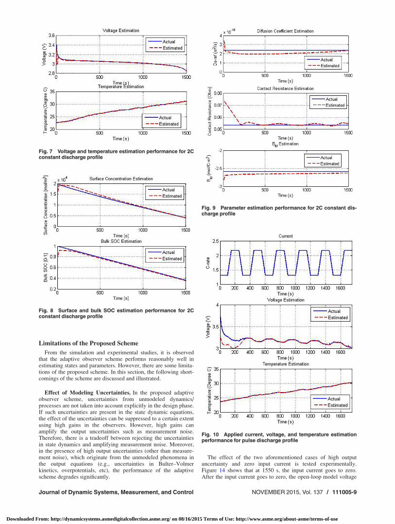
Two sets of experimental studies have been performed basedon two different current profiles. In the first study, a constant cur-rent discharge 2C is used. The results for this study are given inFig. 7 (voltage and temperature estimation), Fig. 8 (surface andbulk SOC), and Fig. 9 (parameter estimation). As expected, theestimated variables converged to a bounded error ball startingwith incorrect initialization. Note that the voltage and temperatureestimates have almost negligible steady-state error as should beexpected given the measured output variables involve the samestates. However, the steady-state error of the unmeasured statesand of the parameter estimates is relatively larger.

In the second experimental study, a pulse discharge profile isapplied to the cell. The results for this study are given in Figs. 10(voltage and temperature estimation), 11 (surface and bulk SOC),and 12 (parameter estimation), respectively. Similar to the first ex-perimental study, the estimated variables converged to a boundederror ball starting with incorrect initialization.

Fig. 5 Bulk SOC and surface concentration estimationperformance

Fig. 6 Parameter estimation performance

Table 1 Model parameters (“F” denotes fitted values)

Parameters Values

D�s;ref 2:4� 10�15 m2=s (F)iþ0 0:0036 A=m2 (F)i�0 0:6102 A=m2 (F)Rf 0:0532 X (F)k1 �0:9442 (F)k2 22; 799 mol=m3 (F)a�s 3:48� 105 m2=m3 [50]e�s 0:58 [41]R� 5� 10�6 m [50]A 0:18 m2 [50]L� 3:4� 10�5 m [50]cþs;max 22; 806 mol=m3 [52]c�s;max 30; 555 mol=m3 [53]qv 0:07 kg [50]Cp 1100 J=kg K [50]hA 0:07 W=K (F)



Limitations of the Proposed Scheme

From the simulation and experimental studies, it is observedthat the adaptive observer scheme performs reasonably well inestimating states and parameters. However, there are some limita-tions of the proposed scheme. In this section, the following short-comings of the scheme are discussed and illustrated.

Effect of Modeling Uncertainties. In the proposed adaptiveobserver scheme, uncertainties from unmodeled dynamics/processes are not taken into account explicitly in the design phase.If such uncertainties are present in the state dynamic equations,the effect of the uncertainties can be suppressed to a certain extentusing high gains in the observers. However, high gains canamplify the output uncertainties such as measurement noise.Therefore, there is a tradeoff between rejecting the uncertaintiesin state dynamics and amplifying measurement noise. Moreover,in the presence of high output uncertainties (other than measure-ment noise), which originate from the unmodeled phenomena inthe output equations (e.g., uncertainties in Bulter–Volmerkinetics, overpotentials, etc), the performance of the adaptivescheme degrades significantly.

The effect of the two aforementioned cases of high outputuncertainty and zero input current is tested experimentally.Figure 14 shows that at 1550 s, the input current goes to zero.After the input current goes to zero, the open-loop model voltage

Fig. 7 Voltage and temperature estimation performance for 2Cconstant discharge profile

Fig. 8 Surface and bulk SOC estimation performance for 2Cconstant discharge profile

Fig. 9 Parameter estimation performance for 2C constant dis-charge profile

Fig. 10 Applied current, voltage, and temperature estimationperformance for pulse discharge profile



cannot track the actual voltage, which is evident from the secondsubplot of Fig. 14. This indicates the presence of high outputuncertainty where the model output has a significant deviationfrom the actual output. Due to the effect of the high output uncer-tainty, the estimates of the states and the parameters starteddiverging after 1550 s which is shown in the third subplot ofFig. 14. Therefore, this illustration shows that the scheme loses itseffectiveness under the aforementioned scenarios. Another factnoted from this illustration is that like other estimation algorithms,persistence of excitation is required for the convergence of theestimates for this proposed approach. This fact is observed in thisillustration where in case of zero applied current the convergenceis poor.

High Initial Error in BM Estimation. During experimentaland simulation studies, one observation we made is that the over-all performance of the adaptive scheme degrades with high initialerror ~BM. In Fig. 13, one such scenario is illustrated under 2C con-stant discharge current. The variable BM is initialized with 50%error. Note that the surface concentration, contact resistance, andvoltage estimation computed via Observer I are reasonably good.However, the performance of Observer II degrades significantlyas evident from the diverging errors in the Bulk SOC estimate anddiffusion coefficient estimates. The probable reason for thisdegraded performance lies in the fact that the reduced model isonly locally identifiable or observable. This limitation of thedesign can be easily overcome by minimizing the initial error inBM with accurate accounting for the initial active material volumefraction of the specific battery cell.

Fig. 11 Surface and bulk SOC Estimation performance forpulse discharge profile

Fig. 12 Parameter estimation performance for pulse dischargeprofile

Fig. 13 Performance of the adaptive observer scheme in pres-ence of output uncertainties and absence of input current

Fig. 14 Percentage errors in state and parameter estimationwith high initial error in ~BM



Conclusion

In this paper, an adaptive observer design is presented for si-multaneous state and parameter estimation of a Li-ion battery cell.It addresses the combined estimation of SOC and some electro-chemical parameters, namely, diffusion coefficient, contact resist-ance, and active material volume fraction of the negativeelectrode, which are key requirements for advanced BMS. Theproposed design considers the coupling between electrochemicaland thermal dynamics of the cell. The design is split into two cas-caded observers each of which is designed based on Lyapunov’sstability analysis. A systematic approach is provided for the selec-tion of the relevant gains of the design. Simulation and experi-mental studies are included which showed the effectiveness of thedesign in estimating the Li-ion concentration distribution, whichgives both the bulk and surface SOC, and some electrochemicalparameters, with a desired convergence rate and accuracy. Partic-ularly, from the experimental studies it is found that the steady-state bulk SOC and surface concentration estimation errors liewithin 5%. The parameter estimation steady-state error for contactresistance and diffusion coefficient lies within 15% and 5%,respectively. In case of BM estimation error, the steady-state erroris around 2%, however, at the cost of smaller initialization error.

However, there are some limitations of this adaptive observerscheme that need special attention in implementation and shouldbe subject to further study. First, a high initial error in the inputcoefficient parameter estimate degrades the performance of thescheme. Second, the stability of the overall scheme is not guaran-teed under persistently zero input current and in the presence oflarge output uncertainties. As another future extension of thiswork, the proposed observer’s performance can be studied underdifferent operating conditions such as higher C-rates and lowtemperature.

Acknowledgment

This research was supported, in part, by the U.S. Department ofEnergy GATE program under Grant No. DE-EE0005571 and NSFunder Grant No. CMMI-1055254.

Nomenclature

A ¼ current collector area (cm2)As ¼ cell surface area exposed to surroundings (cm2)a6

s ¼ specific surface area (cm2/cm3)ce ¼ electrolyte phase Li-ion concentration (mol/cm3)

Cp ¼ specific heat capacity (J/g K)

c6s ¼ solid phase Li-ion concentration (mol/cm3)

c6s;e ¼ solid-phase Li-ion surface-concentration (mol/cm3)

c6s;max ¼ solid-phase Li-ion max. concentration (mol/cm3)

D6s ¼ diffusion coefficient in solid-phase (cm2/s)

D6s;ref ¼ diffusion coefficient at Tref (cm2/s)

E6K ¼ activation energy of diffusion coefficient (J/mol)

E6Ds ¼ activation energy of reaction rate constant (J/mol)

F ¼ Faraday’s constant (C/mol)h ¼ heat transfer coefficient of the cell (W/cm2 K)I ¼ current (A)

K6 ¼ reaction rate constant (cm2.5/mol0.5/s)

K6ref ¼ reaction rate constant at Tref (cm2.5/mol0.5/s)

L6 ¼ length of the cell (cm)r ¼ radial coordinate (cm)R ¼ radius of solid active particle (cm)�R ¼ universal gas constant (J/mol K)

Rf ¼ contact resistance (X)Rf 0 ¼ constant part of contact resistance (X)

T ¼ temperature (K)Tref ¼ reference temperature (K)T1 ¼ temperature of cooling fluid (K)

U6 ¼ open circuit potential (V)a ¼ proportional constant of contact resistance (X/K)

�a6 ¼ charge transfer coefficientv ¼ cell volume (cm3)q ¼ cell density (g/cm3)

Superscript

6 ¼ positive/negative electrode

References[1] Hatzell, K. B., Sharma, A., and Fathy, H. K., 2012, “A Survey of Long-Term

Health Modeling, Estimation, and Control of Lithium-Ion Batteries: Challengesand Opportunities,” American Control Conference (ACC), Montreal, Canada,June 27–29, pp. 584–591.

[2] Saha, B., Goebel, K., Poll, S., and Christophersen, J., 2007, “An IntegratedApproach to Battery Health Monitoring Using Bayesian Regression and StateEstimation,” IEEE Autotestcon Conference, Baltimore, MD, Sept. 17–20, pp.646–653.

[3] Ng, K. S., Moo, C., Chen, Y., and Hsieh, Y., 2009, “Enhanced Coulomb Count-ing Method for Estimating State-of-Charge and State-of-Health of Lithium-IonBatteries,” Appl. Energy, 86(9), pp. 1506–1511.

[4] Plett, G. L., 2004, “Extended Kalman Filtering for Battery Management Sys-tems of LiPB-Based HEV Battery Packs: Part 3. State and ParameterEstimation,” J. Power Sources, 134(2), pp. 277–292.

[5] Remmlinger, J., Buchholz, M., Meiler, M., Bernreuter, P., and Dietmayer, K.,2011, “State-of-Health Monitoring of Lithium-Ion Batteries in Electric Vehiclesby On-Board Internal Resistance Estimation,” J. Power Sources, 196(12), pp.5357–5363.

[6] Kim, I.-S., 2010, “A Technique for Estimating the State of Health of LithiumBatteries Through a Dual-Sliding-Mode Observer,” IEEE Trans. Power Electron.,25(4), pp. 1013–1022.

[7] Gould, C. R., Bingham, C. M., Stone, D. A., and Bentley, P., 2009, “New Bat-tery Model and State-of-Health Determination Through Subspace ParameterEstimation and State-Observer Techniques,” IEEE Trans. Veh. Technol., 58(8),pp. 3905–3916.

[8] Chaturvedi, N. A., Klein, R., Christensen, J., Ahmed, J., and Kojic, A., 2010,“Algorithms for Advanced Battery-Management Systems,” IEEE Control Syst.Mag., 30(3), pp. 49–68.

[9] Doyle, M., Fuller, T. F., and Newman, J., 1993, “Modeling of GalvanostaticCharge and Discharge of the Lithium/Polymer/Insertion Cell,” J. Electrochem.Soc., 140(6), pp. 1526–1533.

[10] Kehs, M. A., Beeney, M. D., and Fathy, H. K., 2014, “Computational Efficiencyof Solving the DFN Battery Model Using Descriptor Form With Legendre Poly-nomials and Galerkin Projections,” American Control Conference (ACC), Port-land, OR, June 4–6, pp. 260–267.

[11] Smith, K. A., Rahn, C. D., and Wang, C., 2010, “Model-Based ElectrochemicalEstimation and Constraint Management for Pulse Operation of Lithium IonBatteries,” IEEE Trans. Control Syst. Technol., 18(3), pp. 654–663.

[12] Klein, R., Chaturvedi, N. A., Christensen, J., Ahmed, J., Findeisen, R., andKojic, A., 2013, “Electrochemical Model Based Observer Design for aLithium-Ion Battery,” IEEE Trans. Control Syst. Technol., 21(2), pp. 289–301.

[13] Forman, J. C., Bashash, S., Stein, J. L., and Fathy, H. K., 2011, “Reduction ofan Electrochemistry-Based Li-Ion Battery Model Via Quasi-Linearization andPade Approximation,” J. Electrochem. Soc., 158(2), pp. A93–A101.

[14] Docimo, D. J., Ghanaatpishe, M., and Fathy, H. K., 2014, “Development andExperimental Parameterization of a Physics-Based Second-Order Lithium-IonBattery Model,” ASME Paper No. DSCC2014-6270.

[15] Santhanagopalan, S., and White, R. E., 2006, “Online Estimation of the State ofCharge of a Lithium Ion Cell,” J. Power Sources, 161(2), pp. 1346–1355.

[16] Domenico, D., Stefanopoulou, A., and Fiengo, G., 2010, “Lithium-Ion BatteryState of Charge and Critical Surface Charge Estimation Using an Electrochemi-cal Model-Based Extended Kalman Filter,” ASME J. Dyn. Syst., Meas., Con-trol, 132(6), p. 061302.

[17] Moura, S. J., Chaturvedi, N. A., and Krstic, M., 2012, “PDE Estimation Techni-ques for Advanced Battery Management Systems—Part I: SOC Estimation,”American Control Conference (ACC), pp. 559–565.

[18] Dey, S., and Ayalew, B., 2014, “Nonlinear Observer Designs for State-of-Charge Estimation of Lithium-Ion Batteries,” American Control Conference(ACC), Portland, OR, June 4–6, pp. 248–253.

[19] Dey, S., Ayalew, B., and Pisu, P., “Nonlinear Robust Observers for State-of-Charge Estimation of Lithium-Ion Cells Based on a Reduced ElectrochemicalModel,” IEEE Trans. Control Syst. Technol. (online).

[20] Samadi, M. F., Alavi, S. M., and Saif, M., 2013, “Online State and ParameterEstimation of the Li-Ion Battery in a Bayesian Framework,” American ControlConference (ACC), Washington, DC, June 17–19, pp. 4693–4698.

[21] Schmidt, A. P., Bitzer, M., Imre, �A. W., and Guzzella, L., 2010, “Model-BasedDistinction and Quantification of Capacity Loss and Rate Capability Fade inLi-Ion Batteries,” J. Power Sources, 195(22), pp. 7634–7638.

[22] Fang, H., Wang, Y., Sahinoglu, Z., Wada, T., and Hara, S., 2013, “AdaptiveEstimation of State of Charge for Lithium-Ion Batteries,” American ControlConference (ACC), pp. 3485–3491.

[23] Fang, H., Wang, Y., Sahinoglu, Z., Wada, T., and Hara, S., 2014, “State ofCharge Estimation for Lithium-Ion Batteries: An Adaptive Approach,” ControlEng. Pract., 25, pp. 45–54.



http://dx.doi.org/10.1109/ACC.2012.6315578

http://dx.doi.org/10.1109/AUTEST.2007.4374280

http://dx.doi.org/10.1016/j.apenergy.2008.11.021

http://dx.doi.org/10.1016/j.jpowsour.2004.02.033


http://dx.doi.org/10.1109/TPEL.2009.2034966

http://dx.doi.org/10.1109/TVT.2009.2028348

http://dx.doi.org/10.1109/MCS.2010.936293

http://dx.doi.org/10.1109/MCS.2010.936293

http://dx.doi.org/10.1149/1.2221597

http://dx.doi.org/10.1149/1.2221597


http://dx.doi.org/10.1109/TCST.2009.2027023


http://dx.doi.org/10.1149/1.3519059

http://dx.doi.org/10.1115/DSCC2014-6270


http://dx.doi.org/10.1115/1.4002475

http://dx.doi.org/10.1115/1.4002475





http://dx.doi.org/10.1016/j.conengprac.2013.12.006


[24] Moura, S. J., Chaturvedi, N. A., and Krstic, M., 2013, “Adaptive PDE Observerfor Battery SOC/SOH Estimation Via an Electrochemical Model,” ASME J.Dyn. Syst., Meas., Control, 136(1), p. 011015.

[25] Wang, Y., Fang, H., Sahinoglu, Z., Wada, T., and Hara, S., 2013, “NonlinearAdaptive Estimation of the State of Charge for Lithium-Ion Batteries,” 52ndAnnual Conference on Decision and Control, pp. 4405–4410.

[26] Wang, Y., Fang, H., Sahinoglu, Z., Wada, T., and Hara, S., 2015, “Adaptive Esti-mation of the State of Charge for Lithium-Ion Batteries: Nonlinear GeometricObserver Approach,” IEEE Trans. Control Syst. Technol., 23(3), pp. 948–962.

[27] Dey, S., Ayalew, B., and Pisu, P., 2014, “Combined Estimation of State-of-Charge and State-of-Health of Li-Ion Battery Cells Using SMO on Electro-chemical Model,” 13th International Workshop on Variable Structure Systems,Nantes, France, June 29–July 2, pp. 1–6.

[28] Zhou, X., Ersal, T., Stein, J. L., and Bernstein, D. S., 2013, “Battery HealthDiagnostics Using Retrospective-Cost Subsystem Identification: Sensitivity toNoise and Initialization Errors,” ASME Paper No. DSCC2013-3953.

[29] Zhou, X., Ersal, T., Stein, J. L., and Bernstein, D. S., 2014, “Battery State of HealthMonitoring by Side Reaction Current Density Estimation Via Retrospective-CostSubsystem Identification,” ASME Paper No. DSCC2014-6254.

[30] Debert, M., Colin, G., Bloch, G., and Chamaillard, Y., 2013, “An ObserverLooks at the Cell Temperature in Automotive Battery Packs,” Control Eng.Pract., 21(8), pp. 1035–1042.

[31] Lin, X., Perez, H. E., Mohan, S., Siegel, J. B., Stefanopoulou, A. G., Ding, Y.,and Castanier, M. P., 2014, “A Lumped-Parameter Electro-Thermal Model forCylindrical Batteries,” J. Power Sources, 257, pp. 1–11.

[32] Lin, X., Perez, H. E., Siegel, J. B., Stefanopoulou, A. G., Li, Y., Anderson, R. D.,Ding, Y., and Castanier, M. P., 2013, “Online Parameterization of Lumped ThermalDynamics in Cylindrical Lithium Ion Batteries for Core Temperature Estimationand Health Monitoring,” IEEE Trans. Control Syst. Technol., 21(5), pp. 1745–1755.

[33] Kim, Y., Mohan, S., Siegel, J. B., Stefanopoulou, A. G., and Ding, Y., 2014,“The Estimation of Temperature Distribution in Cylindrical Battery CellsUnder Unknown Cooling Conditions,” IEEE Trans. Control Syst. Technol.,22(6), pp. 2277–2286.

[34] Lin, X., Fu, H., Perez, H. E., Siegel, J. B., Stefanopoulou, A. G., Ding, Y., andCastanier, M. P., 2013, “Parameterization and Observability Analysis of Scal-able Battery Clusters for Onboard Thermal Management,” Oil Gas Sci. Tech-nol., 68(1), pp. 165–178.

[35] Tanim, T. R., Rahn, C. D., Wang, C.-Y., 2015, “State of Charge Estimation of aLithium Ion Cell Based on a Temperature Dependent and Electrolyte EnhancedSingle Particle Model,” Energy, 80(1), pp. 731–739.

[36] Klein, R., Chaturvedi, N. A., Christensen, J., Ahmed, J., Findeisen, R., andKojic, A., 2010, “State Estimation of a Reduced Electrochemical Model of aLithium-Ion Battery,” American Control Conference (ACC), Baltimore, MD,June 30–July 2, pp. 6618–6623.

[37] Bandhauer, T. M., Garimella, S., and Fuller, T. F., 2011, “A Critical Review of Ther-mal Issues in Lithium-Ion Batteries,” J. Electrochem. Soc., 158(3), pp. R1–R25.

[38] Dey, S., Ayalew, B., and Pisu, P., 2014, “Adaptive Observer Design for aLi-Ion Cell Based on Coupled Electrochemical-Thermal Model,” ASME PaperNo. DSCC2014-5986.

[39] Guo, M., Sikha, G., and White, R. E., 2011, “Single-Particle Model for aLithium-Ion Cell: Thermal Behavior,” J. Electrochem. Soc., 158(2), pp.A122–A132.

[40] Ramadass, P., Haran, B., White, R., and Popov, B. N., 2003, “MathematicalModeling of the Capacity Fade of Li-Ion Cells,” J. Power Sources, 123(2), pp.230–240.

[41] Smith, K., and Wang, C. Y., 2006, “Power and Thermal Characterization of aLithium-Ion Battery Pack for Hybrid-Electric Vehicles,” J. Power Sources,160(1), pp. 662–673.

[42] Rahimian, S. K., Rayman, S., and White, R. E., 2013, “Extension of Physics-Based Single Particle Model for Higher Charge–Discharge Rates,” J. PowerSources, 224, pp. 180–194.

[43] Luo, W., Lyu, C., Wang, L., and Zhang, L., 2013, “A New Extension ofPhysics-Based Single Particle Model for Higher Charge–Discharge Rates,”J. Power Sources, 241, pp. 295–310.

[44] Tanim, T. R., Rahn, C. D., and Wang, C. Y., 2014, “A Temperature Dependent,Single Particle, Lithium Ion Cell Model Including Electrolyte Diffusion,”ASME J. Dyn. Syst., Meas., Control, 137(1), p. 011005.

[45] Vetter, J., Nov�ak, P., Wagner, M. R., Veit, C., M€oller, K.-C., Besenhard, J. O.,Winter, M., Wohlfahrt-Mehrens, M., Vogler, C., and Hammouche, A., 2005,“Ageing Mechanisms in Lithium-Ion Batteries,” J. Power Sources, 147(1–2),pp. 269–281.

[46] Cho, Y. M., and Rajamani, R., 1997, “A Systematic Approach to AdaptiveObserver Synthesis for Nonlinear Systems,” IEEE Trans. Autom. Control,42(4), pp. 534–537.

[47] Rajamani, R., and Hedrick, J. K., 1995, “Adaptive Observers for Active Auto-motive Suspensions: Theory and Experiment,” IEEE Trans. Control Syst. Tech-nol., 3(1), pp. 86–93.

[48] Slotine, J. J. E., and Li, W., 1991, Applied Nonlinear Control, Prentice-Hall,Upper Saddle River, NJ.

[49] Narendra, K. S., and Annaswamy, A., 1989, Stable Adaptive Systems, Prentice-Hall, Englewood Cliffs, NJ.

[50] Prada, E., Domenico, D., Creff, Y., Bernard, J., Sauvant-Moynot, V., and Huet,F., 2012, “Simplified Electrochemical and Thermal Model of LiFePO4–GraphiteLi-Ion Batteries for Fast Charge Applications,” J. Electrochem. Soc., 159(9), pp.A1508–A1519.

[51] Arora, P., Doyle, M., Gozdz, A. S., White, R. E., and Newman, J., 2000,“Comparison Between Computer Simulations and Experimental Data for High-Rate Discharges of Plastic Lithium-Ion Batteries,” J. Power Sources, 88(2), pp.219–231.

[52] Delacourt, C., and Safari, M., 2011, “Analysis of Lithium Deinsertion/Insertionin LiyFePO4 With a Simple Mathematical Model,” Electrochim. Acta, 56(14),pp. 5222–5229.

[53] Santhanagopalan, S., Guo, Q., Ramadass, P., and White, R. E., 2006, “Reviewof Models for Predicting the Cycling Performance of Lithium Ion Batteries,”J. Power Sources, 156(2), pp. 620–628.

[54] Siegel, J. B., Lin, X., Stefanopoulou, A. G., Hussey, D. S., Jacobson, D. L., andGorsich, D., 2011, “Neutron Imaging of Lithium Concentration in LFP PouchCell Battery,” J. Electrochem. Soc., 158(5), pp. A523–A529.



http://dx.doi.org/10.1115/1.4024801

http://dx.doi.org/10.1115/1.4024801









http://dx.doi.org/10.2516/ogst/2012075

http://dx.doi.org/10.2516/ogst/2012075

http://dx.doi.org/10.1016/j.energy.2014.12.031


http://dx.doi.org/10.1149/1.3515880


http://dx.doi.org/10.1149/1.3521314

http://dx.doi.org/10.1016/S0378-7753(03)00531-7





http://dx.doi.org/10.1115/1.4028154


http://dx.doi.org/10.1109/9.566664

http://dx.doi.org/10.1109/87.370713

http://dx.doi.org/10.1109/87.370713

http://dx.doi.org/10.1149/2.064209jes

http://dx.doi.org/10.1016/S0378-7753(99)00527-3

http://dx.doi.org/10.1016/j.electacta.2011.03.030


http://dx.doi.org/10.1149/1.3566341

nonlinear adaptive observer for a lithium-ion battery s ... applications in...derived from the...

Documents