non-markovianstateaggregationfor reinforcementlearning · 3 featurereinforcementlearning 3.1...

Non-Markovian State Aggregation for

Reinforcement Learning

David Johnston

October 30, 2015

Contents

1 Introduction 1

2 Reinforcement Learning 2

2.1 The Value Function . . . . . . . . . . . . . . . . . . . . . . . . . . . . . . 32.2 Markov Decision Processes . . . . . . . . . . . . . . . . . . . . . . . . . . . 4

3 Feature Reinforcement Learning 5

3.1 Feature Maps . . . . . . . . . . . . . . . . . . . . . . . . . . . . . . . . . . 53.1.1 Notation . . . . . . . . . . . . . . . . . . . . . . . . . . . . . . . . . 63.1.2 State Aggregation and φ-uniformity . . . . . . . . . . . . . . . . . 6

3.2 Counterexamples to Open Problem 10 for V ∗ Aggregation . . . . . . . . . 83.2.1 Transient counterexample . . . . . . . . . . . . . . . . . . . . . . . 83.2.2 Second Counterexample . . . . . . . . . . . . . . . . . . . . . . . . 103.2.3 Experimental Performance of Ergodic Counterexample . . . . . . . 14

4 Using Q-learning on Aggregated State Representations 15

4.1 Generating random aggregated MDPs . . . . . . . . . . . . . . . . . . . . 154.1.1 Single Action . . . . . . . . . . . . . . . . . . . . . . . . . . . . . . 154.1.2 Multiple Actions . . . . . . . . . . . . . . . . . . . . . . . . . . . . 16

4.2 Experimental Parameters . . . . . . . . . . . . . . . . . . . . . . . . . . . 174.2.1 Q∗ aggregation . . . . . . . . . . . . . . . . . . . . . . . . . . . . . 174.2.2 V ∗ aggregation . . . . . . . . . . . . . . . . . . . . . . . . . . . . . 18

4.3 Results . . . . . . . . . . . . . . . . . . . . . . . . . . . . . . . . . . . . . . 184.4 Dependence on ǫ . . . . . . . . . . . . . . . . . . . . . . . . . . . . . . . . 204.5 Estimating the deviation from a Markovian process . . . . . . . . . . . . . 204.6 non-Markovianity of Randomly Aggregated MDPs . . . . . . . . . . . . . 224.7 State Aggregation with the Mountain Car Problem . . . . . . . . . . . . . 264.8 Experimental Setup . . . . . . . . . . . . . . . . . . . . . . . . . . . . . . 26

1

4.9 Results . . . . . . . . . . . . . . . . . . . . . . . . . . . . . . . . . . . . . . 274.10 Agreement with theoretical limit . . . . . . . . . . . . . . . . . . . . . . . 30

5 Learning the Aggregation 31

5.1 Existing work . . . . . . . . . . . . . . . . . . . . . . . . . . . . . . . . . . 315.2 U-Tree . . . . . . . . . . . . . . . . . . . . . . . . . . . . . . . . . . . . . . 325.3 Exploration Algorithms . . . . . . . . . . . . . . . . . . . . . . . . . . . . 355.4 The MERL Algorithm . . . . . . . . . . . . . . . . . . . . . . . . . . . . . 36

5.4.1 Notation . . . . . . . . . . . . . . . . . . . . . . . . . . . . . . . . . 365.4.2 Algorithm . . . . . . . . . . . . . . . . . . . . . . . . . . . . . . . . 375.4.3 D-step returns for Markov aggregation . . . . . . . . . . . . . . . . 385.4.4 Sample complexity bound for exact Markov aggregation . . . . . . 405.4.5 D-step returns for exact q-value aggregation . . . . . . . . . . . . . 405.4.6 A sample complexity bound for exact q-value aggregation . . . . . 41

6 Conclusion 48

1 Introduction

Reinforcement learning studies agents that operate in environments that provide themwith rewards in response to actions that the agents take. The agent’s aim (and theagent designer’s) is that the agent takes actions that lead to the maximum possible ac-cumulated reward. Reinforcement learning is a very general framework for goal directedlearning; a reinforcement learner must be able to explore an environment sufficientlyto “discover” where to find the maximum reward, and it must be able to learn enoughabout the dynamics of the environment to devise a policy which delivers the maximumreward in expectation. Supervised learning, in contrast, involves extra knowledge of theenvironment by way of examples of desirable behaviour. Unsupervised learning may notinvolve much prior knowledge of the problem domain, but it is not goal-directed.

The generality of the reinforcement learning setting makes it very difficult to design areinforcement learning agent that learns well in every possible environment. Solomonoffinduction [15] has been proposed as a universal solution to the problem of learning thedynamics of any computable environment. Solomonoff induction is, however, incom-putable and so any real agent must at best be an approximation to it. AIXI [1] is areinforcement learning agent built on Solomonoff induction, and achieves universal op-timality in the sense that no agent exists that learns the on-policy dynamics of anyenvironment significantly faster than AIXI. However, it is not clear that AIXI has theright balance of exploration and exploitation[9].

On the other hand, in a restricted class of environments known as finite state fullyobservable Markov Decision Processes (FS-FO-MDPs), relatively simple algorithms such

2

as Q-learning are known to converge to the optimal policy [20]. A recent result due toHutter [2] has suggested that through the use of state aggregation, techniques applicableto FS-FO-MDPs may be applicable to general environments. This report examines theuse of state aggregation in extending the applicability of Q-learning, and investigatesalgorithms for learning a state aggregation.

The report consists of three sections. Section 2 introduces key notation and defini-tions in reinforcement learning and Hutter’s state aggregation results. Section 4 detailsexperiments examining the behaviour of a Q-learning agent on aggregated processes.Finally, section 5 examines algorithms for learning an aggregated representation of theenvironment, including a brief experimental investigation of McCallum’s U-Tree [6] andan extension of the sample complexity bound of MERL [4].

2 Reinforcement Learning

The agent-environment model is a standard conceptual framework for reinforcementlearners and other AI agents[13]. In this model, an agent Π interacts with an environmentP in discrete cycles indexed by a time step t ∈ N. At each time step the agent may takean action a ∈ A, and in response the environment will provide an observation o ∈ O anda reward r ∈ R ⊆ R to the agent. The sequence of observations, rewards and actions upto time t forms the history:

ht := o1r1a1...ot−1rt−1at−1otrt ∈ Ht := (O ×R×A)t−1 ×O ×R

At cycle t+ 1, the agent selects its next action at+1 according to the current history ht.In general, the agent aims to take the action that maximises the expected return, definedas the discounted sum of rewards [18]:

Gt =∞∑

i=t

γi−tri

where γ ∈ [0, 1] is the discount rate. If the problem terminates in finite time, we canadd a terminal cycle T after which all rewards are 0.

The agent Π can be seen as a (possibly stochastic) function from histories to actions,and the environment P as a (possibly stochastic) function from histories and actions toobservations and rewards:

P : H×A → O ×RΠ : H → A

3

We can express the fact that the agent chooses action at given history ht by Π(ht) = at.If the agent chooses actions stochastically, the distribution Π(at|ht) may be used instead.P (ot+1rt+1|htat) refers to the probability that the environment yields observations ot+1

and reward rt+1 given history ht and action at.

2.1 The Value Function

A wide variety of approaches to reinforcement learning are concerned with learning thevalue function. The value function V : H → R maps a history ht to the expected returnunder the agent’s policy Π [18]:

V Π(ht) := EΠP [Gt+1|ht]

Related to this is the action-value or q-value function, defined as the expected return ofhistory ht when taking action at and subsequently following policy Π

QΠ(ht, at) := EΠP [Gt+1|htat]

The value and q-value functions can be written pseudo-recursively as

QΠ(ht, at) = EΠP [rt+1 + γV Π(ht+1)|htat] (1)

V Π(ht) = QΠ(ht,Π(ht)) (2)

We can define the optimal (q-)value functions as the value of history ht (and action at)under the policy which maximises the expected return

V ∗(ht) = maxΠ

V Π(ht)

Q∗(ht, at) = maxΠ

QΠ(ht, at)

These definitions lead to the pseudo-recursive equations

Q∗(ht, at) = EP [rt+1 + γV ∗(ht+1)|htat] (3)

V ∗(ht) = maxa∈A

Q∗(ht, at) (4)

Π∗(ht) ∈ argmaxa∈A

Q∗(ht, at) (5)

The last line is membership because in general there might be multiple actions that leadto the same expected return. As noted earlier, the objective of a reinforcement learning

4

agent is to maximise expected return, and if an agent can learn the optimal q-valuefunction it can do so via equation 5.

These equations have been presented in terms of the histories ht ∈ H, rather than interms of states. Because histories never repeat, hi = hj if and only if i = j and theseforms do not lead to a closed set of equations. In fully general environments, it is difficultto learn value functions from experience.

2.2 Markov Decision Processes

Markov Decision Processes (MDPs) form an important class of environments that permitlearning from experience. In an MDP, the environment is at any time step t in somestate st ∈ S. These states exhibit the Markov property, which informally asserts thatthe history ht affects the probability of transition to the state st+1 and receiving rewardrt+1 only through the current state st and action at:

P (st+1rt+1|htat) = P (st+1rt+1|stat)

To connect the idea of a state with previous notation, we note that in a fully-observableMDP the agent may directly observe the environment’s state, and so there is a bijectivemap between observations o and states s.

P (ot+1rt+1|htat) = P (ot+1rt+1|otat)

If we suppose further that the state (or observation) space is finite, then for sufficientlylong action sequences states must repeat. Together this forms the class of finite-statefully-observable MDPs, for which we can write closed analogues of the pseudo-recursiveequations 2 to 4 known as the Bellman equations. For the optimal (q-)values, theseare

Q∗(ot, at) = EP [rt+1 + γV ∗(ot+1)]

V ∗(ot) = maxa∈A

Q∗(ot, at)

Reinforcement learning algorithms based on temporal difference learning such as Q-learning and the TD(λ) family are known to converge to the optimal policy for finitestate fully observable MDPs [18, 10].

5

3 Feature Reinforcement Learning

3.1 Feature Maps

Many interesting problems are neither fully observable nor finite state. In such environ-ments, naively applying algorithms developed for FS-FO-MDP’s cannot be expected toproduce acceptable performance.

One approach to dealing with problems like this is to develop a feature map φ : H → Sthat takes the history ht and maps it to a state st that, ideally, summarises all therelevant information of the history ht with respect to developing a policy.

Ideally, the map φ will have enough state distinctions that the agent can eventuallylearn to take the best action given the information it has access to, but not too manymore than this, as a proliferation of states will slow learning. Given that simple agentsperform well on MDPs, we might guess that reducing an environment to an MDP mightbe a reasonable goal. Reducing the environment to a FS-FO-MDP will allow an agentto learn an optimal policy, but as we will discuss later this is a stronger condition thannecessary.

Formally, we will consider feature maps φ : H → S. This induces a reduced process Pφ

on the environment

Pφ(st+1rt+1|htat) =∑

ot+1:φ(htatot+1rt+1)=st+1

P (ot+1rt+1|htat)

Such a process is Markov if Pφ is the same for all histories mapped to the same state

Pφ ∈ MDP⇔ ∃p : Pφ(st+1rt+1|htat) = p(st+1rt+1|stat) ∀ht : φ(ht) = st (6)

The process Pφ may not be Markov. We can, however define a Markove process p througha stochasitic inverse B(h|sa). Formally, we require of B only that

∑

h∈sB(h|sa) = 1.The Markovian process p is defined as follows

P (ht+1|sa) =∑

h∈sB(h|sa)P (ht+1|hta)

p(s′|sa) =∑

h∈s′P (ht+1|sa)

Note the process p is related to, but not the same as the possibly non-Markovian processPφ. Nonetheless, Hutter has established that under appropriate conditions (defined

6

later), the value function of the process p will match the value function of the originalprocess P [2].

3.1.1 Notation

Π∗, V ∗, Q∗ refer to the optimal policy, value and q-value functions of the unaggregatedprocess P .

π∗, v∗ and q∗ refer to the optimal policy, value and q-value functions of the process p.

The shorthand ∀φ(h) = φ(h) may be used to indicate ∀h, h : φ(h) = φ(h).

3.1.2 State Aggregation and φ-uniformity

Given a process P and feature map φ, as defined above, Hutter [2] has shown that sucha map that respects the conditions

|Q∗(h, a)Q∗(h, a)| ≤ ǫ for all φ(h) = φ(h) (7)

Π∗(h) = Π∗(h) for all φ(h) = φ(h) (8)

will have the following properties:

(i) |Q∗(h, a)− q∗(π(h), a)| ≤ ǫ

1− γand |V ∗(h, a)− v∗(π(h), a)| ≤ ǫ

1− γ

(ii) 0 ≤ V ∗(h)− V Π(h) ≤ 2ǫ

(1− γ)2where Π(h) = π∗(φ(h))

(iii) If ǫ = 0 then Π∗(h) = π∗(φ(h))

If ǫ = 0, we refer to the aggregation as exact. Otherwise, it is called approximate.

If a process P , under a map φ, respects equations 7 and 8, then we will say it’s q-valuefunction is φ-uniform.

Similarly, for a map which respects

|V ∗(h, a)− V ∗(h, a)| ≤ ǫ for all φ(h) = φ(h)

Π(h) = Π(h) for all φ(h) = φ(h)

we have the following properties:

(i) |V ∗(h)− v∗(φ(h)) ≤ 3ǫ(1− γ)2 and 〈q∗(φ(h), a)− 〈Q∗(h, a)〉B| ≤3ǫγ

P(1− γ)2

(ii) If ǫ = 0 then Π∗(h) = π∗(φ(h))

7

Here 〈〉B represents the expectation under the dispersion probability B.

Note that in the approximate case for a φ-uniform value function, there is no bound onthe difference between V ∗(h) and V Π(h). Open problem 10 of [2] asks if it is possible toestablish a similar bound as for Q∗ aggregation in this case, and it will be demonstratedthat this is not the case.

Given a process P that has a φ-uniform q-value function under a map φ, the aboveresults establish that learning the q-value function of the related process p will be suf-ficient to (approximately) learn the q-value function of P . The question then is, can areinforcement learning agent like Q-learning in such an environment, using an aggrega-tion φ, learn the q-value function of p? The actual process experienced by such an agentwill be Pφ rather than p, which is not necessarily Markovian, so this is beyond the classof problems for which Q-learning is known to work. Nonetheless, Q-learning has beenobserved to converge on non-Markovian problems, and a proof that it does so under theconditions described is in development.

8

3.2 Counterexamples to Open Problem 10 for V ∗ Aggregation

Here two counterexamples are presented to the following proposition:

Supposing that Π∗(h) = Π∗(h) and |V ∗(h)− V ∗(h)| ≤ ǫ for all h such that φ(h) = φ(h),

can we establish a bound on V Π(h) of the form:

V ∗(h)− V Π(h)?= O

(

ǫ

(1− γ)?

)

(9)

Before presenting the problems, we will note that we can establish some related bounds.Given stochastic inverse B, from [2] we have

〈V Π(h)〉B ≥ V ∗(h)− 3ǫ

(1− γ)2(10)

For this bound on the expectation to hold, we must have V Π(h) not much smaller thanV ∗(h) with high probability. Thus both of the counterexamples construct an MDPwhich, under aggregation, there is a particular history hl that is encountered with verylow probability for which V ∗(h)− V Π(h) can be very large.

Because the counterexamples are constructed from MDPs which are more naturallydescribed in terms of states than histories, we will adopt the terminology of “raw state”to refer to any state of the original MDP, symbolised by capital letters A,B,C, ..., and“aggregated state” to refer to any state in the codomain of φ, symbolised by φ(·). A rawstate A can be understood to be any history that ends in the state A, so we do not losegenerality by switching to this terminology.

3.2.1 Transient counterexample

This example is due to Jan Leike. The actions, transition probabilities and rewards forthe raw MDP are given in Fig. 1.

For this problem, Π∗(C) = Π∗(D) = β. Under this policy:

9

φ(C)

φ(F )

φ(H)

C E F

D G H

0

β−Rα

β

0

α

0

1 + ǫ

1

α, β

α, β

1− γǫ

α, β

1 + ǫ

Figure 1: The first counterexample. All transition probabilities are 1. R is understoodto be a large positive number.

V ∗(E) =1

1− γ+ ǫ

V ∗(G) =1

1− γ

V ∗(F ) =1

1− γ

V ∗(H) =1

1− γ+ ǫ

V ∗(C) = V ∗(D) =γ

1− γ+ γǫ

We will define the stochastic inverses B(F |φ(F )) = 1, and B(H|φ(H)) = 1/2 andB(C|φ(C)) = 0

10

Returning to the problem description, the value functions of φ(H) and φ(F ) will be:

v∗(φ(F )) = V ∗(F ) =1

1− γ

v∗(φ(H)) =1

2(1 + ǫ+ 1− γǫ) + γv∗(φ(H))

=1

1− γ+

ǫ

2

= v∗(φ(F )) +ǫ

2

Given this, we can calculate q-value functions of φ(C):

q∗(φ(C), β) = γv∗(φ(F ))

q∗(φ(C), α) = γv∗(φ(H))

Clearly, π∗(φ(C)) = α. If π∗(φ(C)) = Π(C) = a, then V Π(C) = −R1−γ

, which can bemade arbitrarily large in magnitude for any γ, and so we can find an arbitrarily largedifference in V ∗ − V Π.

3.2.2 Second Counterexample

The above counterexample relies on the stochastic inverse of the raw state C being 0.This second counterexample establishes that 9 can be violated even when the stochasticinverse of the raw state (or history) in question is finite under the optimal policy. TheMDP graph is given in Fig 2. There are two actions available in raw states A and B,and one in the rest; the transition probabilities for these actions are given in the graph,but to keep the diagram clear other transitions have been omitted.

The transition probabilities for the raw states C,D,E and F is equal, such that it isgiven by:

T A = T C = T E =1− δ

3T B = δ

Where can be substituted for any of C,D,E, F , and δ ≪ 1.

11

C A E

D B F

φ(C) φ(A) φ(E)

action = α

TAD, TBD = 1

action = β

TAF , TBF = 1

Figure 2: The second counterexample. Note that only transitions from nodes A and Bare affected by choosing action α or β. The rewards for the various transitionsare given in the text.

The problem has a high degree of symmetry, so the values of nodes C,D,E and F areall given by a similar expression:

V Π( )(CDEF ) = Σa∈Π,s′R s′ + γ(T AVΠ(A) + T BV

Π(B) + T CVΠ(C) + T EV

Π(E))

Where, is substituted for the state of interest, and Σs′R = R A + R B + R C + R D

is the sum of the rewards for the transitions from that node under action a. Becausethey have common transition probabilities, the value for each state depends only on theimmediate reward given, regardless of γ.

12

The rewards for each transition are as follows:

RaAs′ = 0 all a, s′

RαBD = 0

RβBF = −r

RCs′ = −ǫ

6all a, s′

RDs′ =ǫ

12all a, s′

REs′ =ǫ

6all a, s′

RFs′ = −ǫ

12all a, s′

The action superscript has been ommitted for each state that only has one action, anda ∈ α, β.

The values of raw states A and B are given by:

V Π(A) = γ(Π(α|A)V Π(D) + Π(β|A)V Π(F ))

V Π(B) = −Π(β|B)r + γ(Π(α|B)V Π(D) + π(β|B)V Π(F ))

It can be verified that, for any policy Π,

V Π(D)− V Π(C) = ǫ (11)

V Π(D)− V Π(F ) =2ǫ

3(12)

V Π(F )− V Π(E) = −ǫ (13)

From this, we can see that Π∗(A) = Π∗(B) = α, so we also have

V ∗(A) = V ∗(B) = V ∗(D) (14)

V ∗(B)− V β(B) = r (15)

Together, this establishes |V ∗(h)− V ∗(h)| ≤ ǫ for any h, h ∈ φ(h), and that the value ofraw state B differs by r between actions α and β.

We will now show that we can find a value δ such that for any ǫ and γ, r can be arbitrarilylarge and the optimal policy of the aggregated problem will be π(φ(A)) = β.

To find the values of the aggregated states, we will use the stationary distributions ρα

and ρβ of the MDP for the stochastic inverses B(h|sa) under the policies Π(·) = α and

13

Π(·) = β.

ρα =1

N[1,

3δ

1− δ, 1,

1 + 2δ

1− δ, 1, 0]

ρβ =1

N[1,

3δ

1− δ, 1, 0, 1,

1 + 2δ

1− δ]

Where N is a normalising factor. From this, we can see that

action = α action = β

B(A|φ(A)) 1−δ1+2δ

1−δ1+2δ

B(B|φ(A)) 3δ1+2δ

3δ1+2δ

B(C|φ(C)) 1−δ2+δ

1

B(D|φ(C) 1+2δ2+δ

0

B(E|φ(E)) 1 1−δ2+δ

B(F |φ(F )) 0 1+2δ2+δ

Table 1: Stochistic inverses for counterexample 2.

With these inverses, we find that

vβ(φ(E))− vα(φ(C)) =2ǫ

3(2 + δ)

And therefore

vβ(φ(A))− vα(φ(A)) = B(B|φ(A))(−r) + γ(vβ(φ(E))− vα(φ(C))) (16)

vβ(φ(A))− vα(φ(A)) = − 3δ

1 + 2 deltar + γ

2ǫ

3(2 + δ)(17)

To satisfy the assumptions of a counterexample, we want to find values of ǫ, δ and r sothat π(φ(A)) = β is the optimal policy of the aggregated MDP, which will happen ifvβ(φ(A))− vα(φ(A)) > 0. This gives us the following condition:

3δr

1 + 2δ<

2ǫγ

3(2 + δ)

This will be satisfied when

δr <2

27ǫγ (18)

14

Table 2: Q-values of the raw and aggregated problem after 1e5 steps of Q-learning.

State Qα Qβ

A 1.45·10−2 −1·10−2

B 1.45·10−2 −1.01C −4.62·10−2 −4.62·10−2

D 2.79·10−2 2.89·10−2

E 5.4·10−2 5.39·10−2

F −2.12·10−2 −2.05·10−2

State Qα Qβ

φ(A) −2.72·10−2 −3.96·10−4

φ(C) −5.47·10−2 −5.47·10−2

φ(E) 5.06·10−3 5.08·10−3

3.2.3 Experimental Performance of Ergodic Counterexample

The second counterexample above was implemented and a Q-learning agent was used tolearn the value functions of the raw and aggregated problems. The parameters chosenwere ǫ = 0.3, δ = 10−3, γ = 0.5 and r = 1. The Q-learning agent learned the q-valuefunction with a random action selection and a step size α = 1

nat step n.

The agent learned a q-value function which corresponded to the important features ofthe example above: in the raw case, V ∗(A) = V α(A) > V β(A) and V ∗(B) = V α(B) >V β(B), while in the aggregated case V β(φ(A)) > V α(φ(A)). In addition, V ∗(h) −V ∗(h) < 10−1 for all h, h ∈ φ(h) while V α(φ(A)) − V β(B) ≈ 1 (see Table 1). Thisdifference could in principle be made much larger, but it would require a proportionallysmall δ, which could make it take a long time to learn.

15

4 Using Q-learning on Aggregated State Representations

Recall that an environment P that has a φ-uniform q-value for some map φ will preservethe value function of the original problem. As discussed previously, the aggregationφ can induce non-Markovian behaviour in the induced process Pφ (Eq. 6 is violated),which places the task of learning the value function of a general Q∗ aggregated processbeyond the realm in which Q-learning is known to work. Nonetheless, the relationshipbetween the value function of the Markovian process p and the original process P suggestit is worth investigating the applicability of Q-learning to this task. The experimentalinvestigation conducted here has found promising results. Two domains were chosen toinvestigate the performance of Q-learning on aggregated problems:

First, random Markov Decision Processes were generated that admitted Q∗ and V ∗

aggregation. The rate of convergence of Q-learning on the raw MDP was comparedto the rate of convergence of Q-learning operating on the (generally non-Markovian)aggregated problem. This was repeated across many problems with varying parametersto investigate any dependencies that could be found.

Secondly, for a more organic test of value aggregation, an aggregation of the mountaincar task described by Singh [14] was developed from an estimate of the task’s valuefunction.

4.1 Generating random aggregated MDPs

To test the performance of a Q-learning agent on aggregated state representations, ascheme was developed to generate random MDPs with properties that allowed theirstates to be aggregated under Q∗ or V ∗ aggregation.

4.1.1 Single Action

The goal is to generate a transition matrix Tss′ and reward matrix Rss′ for an MDPwhich produces groups of states with the same value that can be aggregated. A singleaction scheme is developed first for simplicity. We begin by specifying an arbitrary valuevector v that satisfies the desired equality properties for Q∗ or V ∗ aggregation. A matrixT is generated with entries selected from Uniform(0, 1). This matrix is verified to beaperiodic and irreducible (and regenerated if it is not), and each row is normalised sothat it sums to 1. Given T and v, we require a reward matrix R to satisfy the Bellman

16

equation:

v(s) =∑

s′

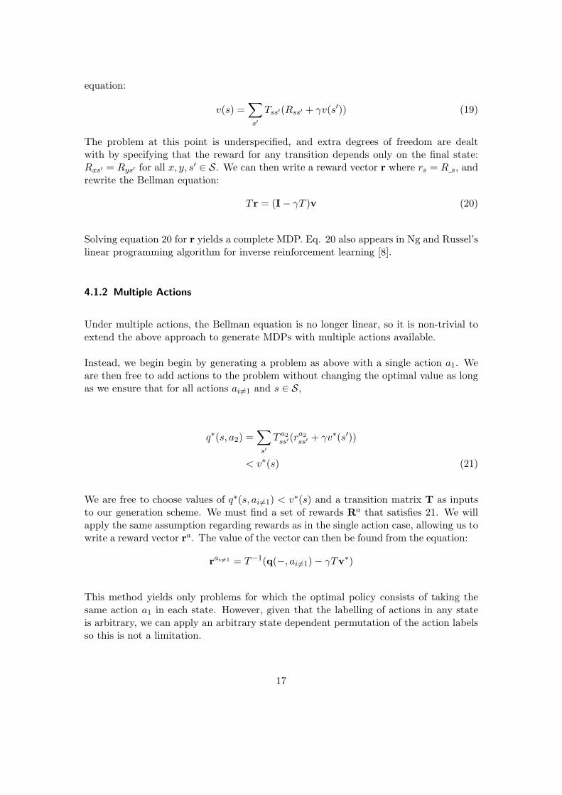
Tss′(Rss′ + γv(s′)) (19)

The problem at this point is underspecified, and extra degrees of freedom are dealtwith by specifying that the reward for any transition depends only on the final state:Rxs′ = Rys′ for all x, y, s

′ ∈ S. We can then write a reward vector r where rs = R s, andrewrite the Bellman equation:

Tr = (I− γT )v (20)

Solving equation 20 for r yields a complete MDP. Eq. 20 also appears in Ng and Russel’slinear programming algorithm for inverse reinforcement learning [8].

4.1.2 Multiple Actions

Under multiple actions, the Bellman equation is no longer linear, so it is non-trivial toextend the above approach to generate MDPs with multiple actions available.

Instead, we begin begin by generating a problem as above with a single action a1. Weare then free to add actions to the problem without changing the optimal value as longas we ensure that for all actions ai 6=1 and s ∈ S,

q∗(s, a2) =∑

s′

T a2ss′(r

a2ss′ + γv∗(s′))

< v∗(s) (21)

We are free to choose values of q∗(s, ai 6=1) < v∗(s) and a transition matrix T as inputsto our generation scheme. We must find a set of rewards Ra that satisfies 21. We willapply the same assumption regarding rewards as in the single action case, allowing us towrite a reward vector ra. The value of the vector can then be found from the equation:

rai 6=1 = T−1(q(−, ai 6=1)− γTv∗)

This method yields only problems for which the optimal policy consists of taking thesame action a1 in each state. However, given that the labelling of actions in any stateis arbitrary, we can apply an arbitrary state dependent permutation of the action labelsso this is not a limitation.

17

4.2 Experimental Parameters

In all cases, the value function is learned using the standard Q-learning algorithm. Theagent begins in state s, takes action a and observes the next state s′ and the reward rass′ .It then updates its estimate of the value of the state-action pair (s, a) as

qi+1(s, a) = qi(s, a) +1

ns,a(rass′ + γmax

a′(qi(s

′, a′))− qi(s, a))

Here, ns,a is the number of times the agent has observed the state action pair (s, a). Thevalue estimate was initialised to q0(−,−) = 0 for all states and actions.

For each generated problem, the Q-learning algorithm was run on the raw MDP and theaggregated MDP for 1e6 steps.

Both Q∗ and V ∗ aggregation were investigated. While counterexamples exist for V ∗

aggregation, it is still of interest whether these are common limitations.

64 problems were generated which represented all possible combinations of the followingparameters when they were allowed to vary in powers of 2 between their minima andmaxima (note that not every available numerical combination yields a possible MDP):

|S| |φ(S)| b |A|min 4 2 2 1

max 64 32 32 8

Where b is the “branching factor” of the transition matrix - the number of transitions outof each state for each particular action. It was required that |Sφ| ≤ |S|/2 and b < |S|.

4.2.1 Q∗ aggregation

For exact Q∗ aggregation, a target value vector v was formed by sampling |Sφ| realnumbers v∗1, ..., v

∗Sφ

from the uniform distribution on (0, 10|Sφ|) and setting the first

|Sφ|/|S)| entries of v to v∗1, the next to v∗2 and so on. For each non-optimal actiona 6= a1 added to the problem, a further |Sφ| real numbers were sampled such thatvij ∼ U(v∗j − 40, v∗j − 1). The values q∗(h, a) were initialised so that the Q-value of eachstate in the same group was identical.

Approximate Q∗ aggregation proceeded in almost the same manner, except a noise ǫ ∼(0, ǫmax) was independently sampled for each state and added to the value function.

18

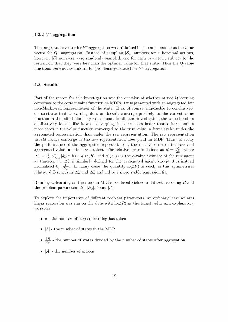
4.2.2 V ∗ aggregation

The target value vector for V ∗ aggregation was initialised in the same manner as the valuevector for Q∗ aggregation. Instead of sampling |Sφ| numbers for suboptimal actions,however, |S| numbers were randomly sampled, one for each raw state, subject to therestriction that they were less than the optimal value for that state. Thus the Q-valuefunctions were not φ-uniform for problems generated for V ∗ aggregation.

4.3 Results

Part of the reason for this investigation was the question of whether or not Q-learningconverges to the correct value function on MDPs if it is presented with an aggregated butnon-Markovian representation of the state. It is, of course, impossible to conclusivelydemonstrate that Q-learning does or doesn’t converge precisely to the correct valuefunction in the infinite limit by experiment. In all cases investigated, the value functionqualitatively looked like it was converging, in some cases faster than others, and inmost cases it the value function converged to the true value in fewer cycles under theaggregated representation than under the raw representation. The raw representationshould always converge as the raw representation does yield an MDP. Thus, to studythe performance of the aggregated representation, the relative error of the raw andaggregated value functions was taken. The relative error is defined as R = ∆r

n∆a

n, where

∆rn = 1

|S|∑

a,s |qn(a, h) − q∗(a, h)| and qrn(a, s) is the q-value estimate of the raw agentat timestep n. ∆a

n is similarly defined for the aggregated agent, except it is insteadnormalised by 1

|Sφ| . In many cases the quantity log(R) is used, as this symmetrises

relative differences in ∆rn and ∆a

n and led to a more stable regression fit.

Running Q-learning on the random MDPs produced yielded a dataset recording R andthe problem parameters |S|, |Sφ|, b and |A|.

To explore the importance of different problem parameters, an ordinary least squareslinear regression was run on the data with log(R) as the target value and explanatoryvariables

• n - the number of steps q-learning has taken

• |S| - the number of states in the MDP

• |S||Sφ| - the number of states divided by the number of states after aggregation

• |A| - the number of actions

19

Regression Coefficients

Parameter n |S| b |A| |S||Sφ| R2

V ∗−aggregation 0.03 -0.14 0.29 0.32 3.00 0.12Q∗−aggregation 0.06 -0.24 0.81 0.17 1.93 0.26

Table 4: Ordinary Least Squares regression on the improvement in performance afforded

0 20 40 60

−2

0

2

4

6

|S||Sφ|

log(R

)

Q∗ aggregation

0 20 40 60

−2

0

2

4

6

|S||Sφ|

V ∗ aggregation

Figure 3: log(R) against |S||Sφ| for V

∗ and Q∗ aggregation. log(R) > 0 implies the aggre-

gated agent outperformed the raw agent.

• b - the number of possible transitions for every (state, action) pair (identical forall problems studied)

All parameters were normalised to take values between 0 and 1 before the regression wasperformed, and a few extreme outliers were filtered out.

The data was randomly partitioned into a training and a test set. The fit was performedon the training set and the variance score R2 calculated on the test set.

From Table 4, it is clear that the most significant effect of the difference in learningrate between the raw and aggregated problems is the “degree of aggregation” (ratio

of |S||Sφ|), with a significantly better fit for Q∗ aggregation. In fact, a model with |S|

|Sφ|as the sole explanatory variable minimised the Bayesian information criterion for bothaggregation types. For Q∗ aggregation, the simple model achieved a BIC of 6 while thebest two-variable model scored 12.5, while analogous models for V ∗ aggregation scored0.5 higher in each case.

20

log(R) is plotted agains |S||Sφ| in Fig. 3. It is apparent from this plot that while the

vast majority of the time the aggregated agent learned the value function faster, therewere some tests for which the aggregated agent performed worse than the raw agent,particularly for low values of |S|

|Sφ| . This could be due either to trial-to-trial variation,

or because some problems were found for which no aggregation consistently performedbetter. To test this, ten problems were selected from those that contributed points belowthe line, and ten repeated trials were run with each. The mean of all trials was 〈R〉 = 2.5with standard deviation σ = 3.0. Only a single problem had a mean R below 1, with〈R〉 = 0.82 and individually σ = 0.74. There is a probability of approximately 0.85 ofgetting at least one result this low if the true means were all above 1. This evidencesuggests that the instances in which the raw agent performed better were due to randomvariation.

4.4 Dependence on ǫ

Problems were separately generated to investigate the change in convergence when noisesampled independently for each state from Uniform(0, ǫmax) was added to the valuefunction. For the problems described above, dependence was usually not visible even forrelatively large values of ǫmax, which may have been because the absolute convergenceof the randomly generated problems was often poor. To get a clearer picture of thedependence on ǫmax, MDPs with |S| = 4, |Sφ| = 2, b = 4 and a = 1 were generated.After 1e4 iterations, these had typically converged to an average deviation from the truevalue function of ∆ ≈ 0.01 − 1, where the state values themselves were between 0 and40.

Under these conditions, some dependence on ǫmax is visible, as can be seen in Fig. 4.The lack of dependence for problems that exhibited slower convergence suggests thatnoise chiefly affects the ultimate precision achieved and not the rate of convergence.

4.5 Estimating the deviation from a Markovian process

The aggregated problems generated here are not necessarily Markovian, but it is in-teresting to investigate how much they deviate from Markov processes in practice. Toestimate this quantity, the degree to which the process conditioned on the two mostrecent states differed from the process conditioned on the most recent state was used.Define a process P with N raw states (“histories”) and an aggregation φ with n aggre-gated states s1, ...sn ∈ Sφ. St indicates the state of the process at time t. The inducedprocess Pφ yields n probability distributions Pφ(St = s|St−1 = s′), and n2 distributionsPφ(St = s|St−1 = s′, St−2 = s′′) where s, s′, s′′ ∈ Sφ. If the process were Markovian, thenPφ(St|St−1 = s′, St−1 = s′′) = Pφ(St|St−1 = s′) for all s, s′, s′′ ∈ Sφ.

21

0 1 2 3 4 5 6 7

1

2

3

ǫmax

R

Dependence of R on ǫmax

Figure 4: When large amounts of noise ǫ have been added to the value function, the rawagent clearly represents the value function with more precision.

Define Dss′ as the Kullback-Liebler divergence between the process conditioned on oneand two timesteps:

Dss′ = DKL(Pφ(St|St−1 = s, St−2 = s′)‖Pφ(St|St−1 = s))

=∑

s′′∈Sφ

Pφ(s′′|s, s′) log Pφ(s

′′|s, s′)Pφ(s′′|s)

Where we use the shorthand Pφ(s|s′) := Pφ(St = s|St−1 = s′).

To calculate the KL divergence, we need to calculate transition probabilities for theaggregated problem. To do this, we will exploit the fact that all aggregated problems weare studying have a stationary distribution ρ(h) under the optimal policy in which every(raw) state has a nonzero occupation. For an agent following the optimal policy, then,

each aggregated state has a well defined stochastic inverse B(h|φ(h)) = ρ(h)∑h′∈φ(s) ρ(h

′)

which is nonzero for all s ∈ φ(s). Define the conditional distribution

ρ(st|φ(st−1)) :=∑

s′∈φ(st−1)

P (st|s′)B(s′|φ(st−1))

We can then find the transition probabilities of the aggregated process by summing over

22

s ∈ φ(st):

Pφ(φ(st)|φ(st−1)) =∑

s′∈φ(st)ρ(s′|φ(st−1))

Defining the second-order stochastic inverse B(st|φ(st), φ(st−1)) =ρ(st|φ(st−1)∑

s′∈φ(st)ρ(s′|φ(st−1))

,

we can follow similar steps to calculate the second-order transition probabilities of theaggregated process:

Pφ(φ(st)|φ(st−1), φ(st−2)) =∑

s′∈φ(st)

∑

s′′∈φ(st−1)

P (s′′|s′)B(s′|φ(st−1), φ(st−1))

If we were analysing problems in which we might find ρ(s) = 0 for all s in some aggre-gated state φ(s), we would need an alternative treatment for aggregated states with 0probability. However, this is not necessary here as ρ(s) > 0 for all s ∈ S for the problemswe will analyse.

The KL divergence is only defined if the first argument is 0 wherever the second argumentis 0. We note above that if Pφ(φ(st)|φ(st−1)) = 0, then ρ(s|φ(st−1)) = 0 for all s ∈ φ(s)and so Pφ(φ(st)|φ(st−1), φ(st−2)) = 0 also. This is not necessarily true in the otherdirection.

Using distributions Pφ calculated from P and φ as described above, we calculate the n2

divergences Dij . To estimate the “non-Markovianity” of the process, we then averagethese D := 1

n2

∑

i = 0n∑n

j=0Dij .

We will finally note that D > 0 implies that an aggregated problem is non-Markovian,but the converse is not true. We are checking the difference between the first and secondorder transitions as a matter of convenience, but a lack of distinguishability based onsecond order transitions doesn’t imply that this is true of higher order transitions.

4.6 non-Markovianity of Randomly Aggregated MDPs

To begin with, I investigated the behaviour of randomly aggregated MDPs with respectto the measure D. A number of MDPs were generated with varying parameters N :=|S|, nagg := Sφ and b the “branching factor” which measures the average number oftransitions from each state. The results are plotted in Fig. 5. There is clearly a strongand highly predictable dependence of D on all three paremeters.

Two general trends which can be seen in the results are that D seems to be maximal fornagg ≈ N/2 and for low b. As expected, D = 0 where N = nagg, because the aggregatedproblem is exactly the same as the raw problem in that case.

23

20 40 60 80 100 1200

1

2

3

·10−2

nagg

D

N = 128, b = 8, nagg varies

20 40 60 80 100 1200

1

2

3

·10−2

N

b = 8, nagg = 8, N varies

10 20 30 40 50 60

1

2

3

·10−2

b

D

N = 128, nagg = 8, b varies

2325

2724

26

28

0

5

·10−2

naggN

D

b = 8, N and nagg vary

Figure 5: Variation of “non-Markovianity” D with parameters N , nagg and b. Pointshave been coloured by value of D in the last plot.

24

An informal reason for why D might peak at nagg ≈ N/2 comes to mind: Knowingφ(st−2) narrows down the number of possible raw states to |φ(st−2)|. Obviously, thisis usually more informative if |φ(st−2)| is small than if it is large. This does not neces-sarily imply that knowing φ(s0)...φ(st−2 is more informative where the average |φ(s)| issmall, though; it could be the case that denser aggregations tend to benefit from longerhistories.

The fact that D increases with decreasing b has a ready explanation. Informally again,a small b means that P (st|st−1) is zero for many choices of st. Given that the remainingprobailities are randomly sampled, this suggests that P (st|st−1) will usually be moresharply peaked where b is small; that is, it will have lower entropy. Holding a fixedB(s|φ(s)), we would then expect a small b to usually give a ρ(st|φ(st−1)) with lowerentropy. In other words, a small b will usually mean that knowing φ(st−1) will give usmore information about st than a similar problem with a large b.

The arguments presented are informal, as the questions addressed are not central to theanalysis in this report. We are concerned with the performance of reinforcement learningagents on aggregated problems, and the degree to which these problems are Markoviandoes not have a strong theoretical bearing on this question.

The key question is whether D has any predictive power regarding the performance ofa Q-learning agent on an aggregated problem. To evaluate this, 70 random aggregatedproblems were generated with N = 32, nagg = 16 and b that varied from 4 to 32 insteps of 4. The choice of fixing N and nagg was made because we know that R dependsstrongly on N/nagg, and we have theoretical reasons unrelated to D to believe it should.R may depend weakly on b, but fixing b also leads to a very restricted range of D, so itwas allowed to vary.

The results of the experiment are plotted in Fig. 6. There does not appear to be anyrelationship between R and D in the data. This test has many caveats and certainlydoes not exclude the possibility that certain types of non-Markovian behaviour pose aproblem to a Q-learning agent. However, it does suggests that if a value function can berepresented by a Q∗-aggregation, whether or not the resulting problem is approximatelyMarkovian does not appear to affect the performace of a Q-learning agent.

Several caveats of using D have already been mentioned. A final significant caveat is thedefinition of Markovian used. Here, the Markovian property of the process is investigatedin terms of the history of aggregated states, while in practice the Markovian property ofinterest is in terms of the history of raw observations. Thus perhaps the more relevantmeasure for the aggregated Markovian processes investigated here is how much better anoutcome (rewards and observations) can be predicted if the agent is given access to theraw state instead of the aggregated state. This should not be too difficult to implement,but due to time constraints it hasn’t been done here.

25

h

1 2 3 4 5 6·10−2

0

1

2

D

log(R

)

Variation of R with D

Figure 6: log(R) against D for a random selection of problems.

26

4.7 State Aggregation with the Mountain Car Problem

The MDPs generated specifically for the task of exploring value aggregation may not bevery similar to any “real” problems in reinforcement learning. For a more natural testof state aggregation, aggregation was applied to the mountain car problem described bySutton and Singh [14].

4.8 Experimental Setup

Figure 7: Diagram of the mountain car task

The mountain car problem, illustrated in Fig. 7, places a stationary car at x ≈ −0.4between two hills, and its goal is to climb the right-hand hill to reach the goal state atx = 0.5. The car may either accelerate forwards, accelerate backwards or coast, but thecar’s engine is weaker than the force from gravity on the steepest slopes of each hill, soit must first travel backwards to build the momentum to escape. For each step that thecar has not reached the exit state, it receives a reward of −1, and for the goal state itreceives a reward of 0. Further details of the problem are described at [16].

To create aggregated states, a close approximation to the true value function of the taskwas required. The state space is continuous, so some sort of function approximationwas required. A tile coding as described in [18][17] with 16 tilings was used as theapproximator. For each episode the car started randomly positioned in the interval(−1.2, 0.5) with random velocity in the interval (−0.07, 0.07). A Q-learning agent reachedthe minimum average episode length after approximately 5000 episodes, and the agentwas executed for a further 25 000 to learn a high fidelity representation of the valuefunction. The value function learned can be seen in Fig. 8.

27

-1.2 -0.8 -0.4 0 0.4

-5

0

5

·10−2

x

x

-1.2 -0.8 -0.4 0 0.4x

−100

−50

Figure 8: Left: Value function learned by the tile-coded Q-learning agent. Right: Visu-alisation of 16 aggregated classes. The classes are delineated by contour lines,and some classes have multiple separated regions. The classes visibly trace thevalue function learned by the tile-coded agent.

This function was then used to generate an aggregation φ(s). First, the state space wasdiscretised into 100×100 equally sized position and velocity states, and a value functionderived from the tile coding estimate was mapped to these cells.

The q-values of each cell form points in R3. To produce an aggregation, K-means

clustering was applied to the cells on the basis of their q-values with a custom metricdesigned for the purpose. The metric ρq : R

3×R3 → R∪{∞} was defined as follows for

two states c1, c2 ∈ R3:

ρq(c1, c2) =

{

∞ π∗(c1) 6= π∗(c2)

maxa |q(c1, a)− q(c2, a)| otherwise

A visualisation of the classes derived using k = 16 classes is presented in Fig. 8.

V ∗ aggregation was also trialled. For V ∗ aggregation, a slightly different metric ρv wasused:

ρv(c1, c2) =

{

∞ π∗(c1) 6= π∗(c2)

|c(c1)− c(c2)| otherwise

4.9 Results

The performance of the aggregated agent with state representation φa(s) was comparedto a discretised agent using a square grid state representation φd(s) with the same total

28

number of states. The relative performance is plotted in Fig. 10 and some key numbersare summarised in the table 9.

|φa(S)| = 16 |φd(S)| = 16

episode length, c = 32 555 5757



ǫ 21 -

|φa(S)| = 64 |φd(S)| = 64




ǫ 10 -

|φa(S)| = 256 |φd(S)| = 256




ǫ 7 -

|φa(S)| = 1024 |φd(S)| = 1024




ǫ 4 -

Figure 9: Average episode lengths for a Q∗ aggregated agent on the mountain car task.|φa(S)| refers to the number of states of the aggregated agent, |φd(S)| refers tothe number of states of the discretised agent and c is the number of completedepisodes. The original tile coded agent had an average episode length of 121once the value function converged.

The performance of Q∗ and V ∗ aggregation was nearly identical given the same numberof target states. Both were able to approximate the value function significantly betterthan a discretised agent with the same number of states, and in many cases betterthan said agent with significantly more states. The coarser aggregations |φa(S)| =16 and |φa(S)| = 64 also exhibited somewhat faster initial convergence than the fineraggregations, though they were ultimately unable to approximate the value function asprecisely.

29

100 101 102 103 104102

103

104

105

episodelength

N = 16

AggregatedDiscretised

100 101 102 103 104102

103

104

105N = 64


100 101 102 103 104102

103

104

105

episodes

episodelength

N = 256


100 101 102 103 104102

103

104

105

episodes

N = 1024


Figure 10: Comparison of gridded and aggregated state representations.

30

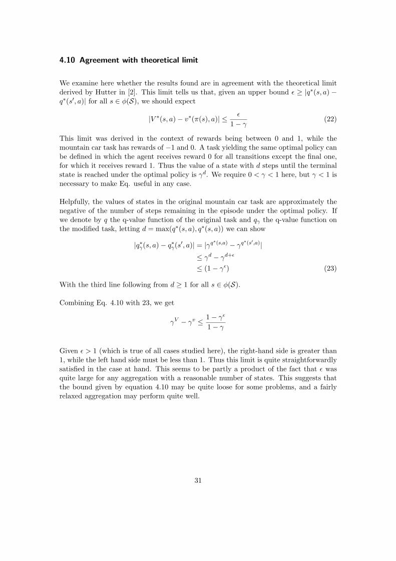
4.10 Agreement with theoretical limit

We examine here whether the results found are in agreement with the theoretical limitderived by Hutter in [2]. This limit tells us that, given an upper bound ǫ ≥ |q∗(s, a) −q∗(s′, a)| for all s ∈ φ(S), we should expect

|V ∗(s, a)− v∗(π(s), a)| ≤ ǫ

1− γ(22)

This limit was derived in the context of rewards being between 0 and 1, while themountain car task has rewards of −1 and 0. A task yielding the same optimal policy canbe defined in which the agent receives reward 0 for all transitions except the final one,for which it receives reward 1. Thus the value of a state with d steps until the terminalstate is reached under the optimal policy is γd. We require 0 < γ < 1 here, but γ < 1 isnecessary to make Eq. useful in any case.

Helpfully, the values of states in the original mountain car task are approximately thenegative of the number of steps remaining in the episode under the optimal policy. Ifwe denote by q the q-value function of the original task and qγ the q-value function onthe modified task, letting d = max(q∗(s, a), q∗(s, a)) we can show

|q∗γ(s, a)− q∗γ(s′, a)| = |γq∗(s,a) − γq

∗(s′,a)|≤ γd − γd+ǫ

≤ (1− γǫ) (23)

With the third line following from d ≥ 1 for all s ∈ φ(S).

Combining Eq. 4.10 with 23, we get

γV − γv ≤ 1− γǫ

1− γ

Given ǫ > 1 (which is true of all cases studied here), the right-hand side is greater than1, while the left hand side must be less than 1. Thus this limit is quite straightforwardlysatisfied in the case at hand. This seems to be partly a product of the fact that ǫ wasquite large for any aggregation with a reasonable number of states. This suggests thatthe bound given by equation 4.10 may be quite loose for some problems, and a fairlyrelaxed aggregation may perform quite well.

31

5 Learning the Aggregation

The work so far discusses the performance of agents on aggregated problems with ag-gregations derived from a precise knowledge of the fundamental problem’s true valuefunction. This is, of course, an unrealistic requirement for any useful agent. If thedesigners already know the value function, they would have little need for an agent tolearn it. It is important to ask how Q∗-aggregation can be used to improve the per-formance of agents when we do not know the value function we wish them to learn.There are two main avenues through which aggregation could help an agent to learn apolicy: first, an aggregation reduces the number of states in a problem, and so the sameamount of exploration will provide more samples per state (this is especially significantif we are comparing an aggregation to a problem working with the entire history, aseach history can have at most one sample). This much has been demonstrated by theexperiments conducted so far, but to take advantage of this we require agents that canlearn an aggregation. Secondly, if an agent performs some sort of search through a spaceof possible environment representations, if we require that the search space contains aQ∗-aggregation of the true environment rather than an exact representation, we may beable to define a smaller space to be searched.

5.1 Existing work

Extensive work exists on agents which learn an adaptive representation of a state space.

Munos and Moore [7] have examined approaches to refining a discretisation of a contin-uous state space. Their approach represents the state space in a structure known as akd-trie that divides the state space into hierarchically organised rectangles and definesa value at the corner of each “leaf” rectangle. The value of a particular point is linearlyinterpolated from the corners that surround it. The state space can be refined by split-ting these rectangles, and the authors test a number of local heuristics for deciding whento do this:

• The average difference in value between the corners of a rectangle

• The variance in the value of the corners of a rectangle

• Policy disagreements between the corners of a rectangle

These local heuristics were found to offer reasonable performance for a 2D car on a hilltask similar but not identical to the mountain car task discussed here, but these heuristicsstruggled in higher dimensions. They also proposed two non-local criteria involvingmeasures they termed influence, that measures the degree to which one state influences

32

other states in the problem, and variance which is the expected squared deviation ofactual returns from the value function of that state. These global measures were found toperform better on higher dimensional tasks. Reynolds [12] employs a method for refiningcontinuous state space discretisations similar to the policy disagreement heuristic trialledby Munos and Moore.

McCallum [6] has developed the U-Tree algorithm for discrete state spaces, which main-tains a tree representation of the state space and uses a statistical test on the transitionsobserved each time a state has been visited to determine if dividing the state couldbetter represent the value function. Uther and Veloso [19] extend U-Tree to continuousstate spaces. A similar approach is taken by Pyeatt and and Howe [11], who instead ofrecording the full history of actions and observations, record the history of value updatesfor each leaf node to decide when to split states.

5.2 U-Tree

McCallum’s U-Tree algorithm represents a model of its environment in a tree, in whichthe leaves represent the states and each internal node is associated with a distinction.An internal node’s distinction maps a partial history hk = o1a1r2...ak−1rkok to exactlyone of that node’s children on the basis of a particular component of observation ok−d

or action ak−d−1 where the time index d is a parameter of the distinction. Thus everypartial history of the agent up to ht is associated with one of the agent’s leaf nodes.

At regular intervals, the agent computes candidate distinctions for each of its leaf nodes.That node is expanded into a number of “fringe nodes”, and partial histories are asso-ciated with the fringe nodes of the candidate distinction. The q-values of each historyare calculated by qp(hk) = rk+1 + γv(φ(hk+1)). If a Kolmogorov-Smirnoff test indicatesthat the values of the histories of different fringe nodes shows sufficient evidence of beingdrawn from different distributions, the candidate distinction is accepted and the fringenodes are converted to leaf nodes.

This heuristic for splitting states attempts to distinguish states that have different q-values, and this aligns it in principle with Q∗-aggregation. In practice the algorithmcannot detect every possible q-value distinction. Distinctions are drawn on the basis ofan observation or action and a time index - for example, a distinction might be drawnon the basis of a component of the ot−3 observation for a given partial history to time t.If there is a relevant distinction to be drawn on the basis of two observation componentsfrom, say ot−3 and ot−2, then U-Tree can learn the distinction iff a relevant distinctioncan be drawn of ot−3 or ot−2 individually. It is possible to modify U-Tree to expand twolayers of fringe nodes, which would permit it to learn all distinctions that require twoobservation components, but increasing the fringe depth comes with an exponential costin computation time and in the number of samples needed to make meaningful tests.

33

Nonetheless, U-Tree is an algorithm that learns value distinctions and, as far as possible,learns only value distinctions, which is what is wanted for a Q∗-aggregation.

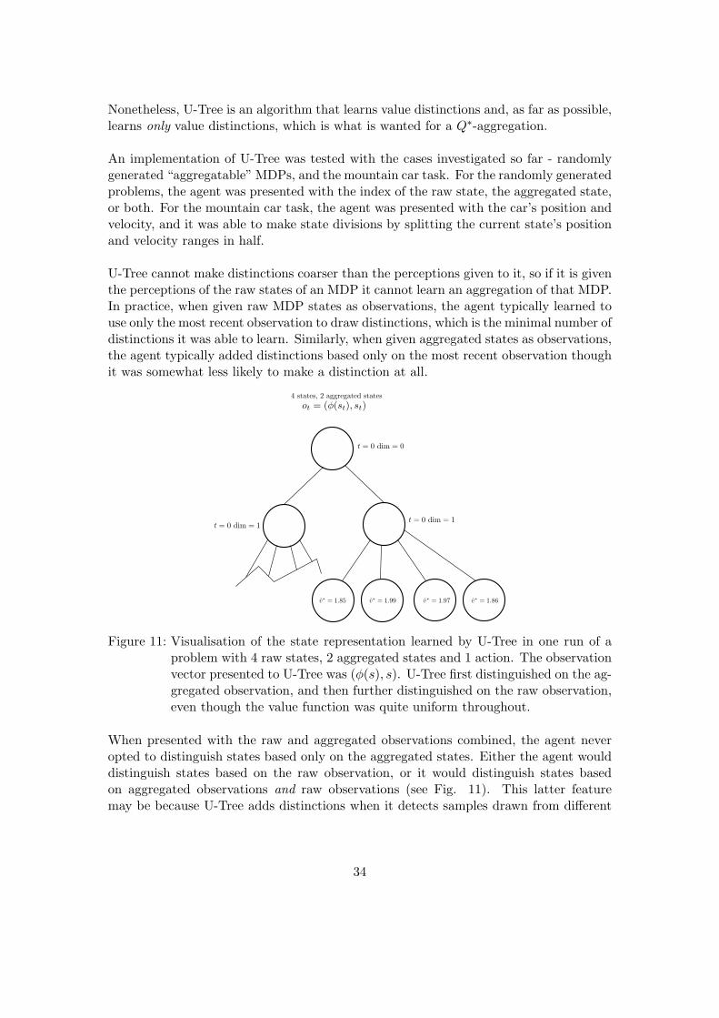
An implementation of U-Tree was tested with the cases investigated so far - randomlygenerated “aggregatable” MDPs, and the mountain car task. For the randomly generatedproblems, the agent was presented with the index of the raw state, the aggregated state,or both. For the mountain car task, the agent was presented with the car’s position andvelocity, and it was able to make state divisions by splitting the current state’s positionand velocity ranges in half.

U-Tree cannot make distinctions coarser than the perceptions given to it, so if it is giventhe perceptions of the raw states of an MDP it cannot learn an aggregation of that MDP.In practice, when given raw MDP states as observations, the agent typically learned touse only the most recent observation to draw distinctions, which is the minimal number ofdistinctions it was able to learn. Similarly, when given aggregated states as observations,the agent typically added distinctions based only on the most recent observation thoughit was somewhat less likely to make a distinction at all.

Figure 11: Visualisation of the state representation learned by U-Tree in one run of aproblem with 4 raw states, 2 aggregated states and 1 action. The observationvector presented to U-Tree was (φ(s), s). U-Tree first distinguished on the ag-gregated observation, and then further distinguished on the raw observation,even though the value function was quite uniform throughout.

When presented with the raw and aggregated observations combined, the agent neveropted to distinguish states based only on the aggregated states. Either the agent woulddistinguish states based on the raw observation, or it would distinguish states basedon aggregated observations and raw observations (see Fig. 11). This latter featuremay be because U-Tree adds distinctions when it detects samples drawn from different

34

0 5 10 15 20 25 300

20

40

number of states

frequen

cyRaw Representation

0 2 4 6 8 10 12 14 160

10

20

30

40

number of states

Aggregated Representation

0 20 40 60 80 100 120 1400

10

20

30

number of states

frequen

cy

Combined Representation

Figure 12: The number of states in the representation learned by U-Tree. The combinedrepresentation was in principle able to settle on an 8-state representation, butit never did.

distributions, even if those distributions have the same mean. The number of statesU-Tree learned is recorded in Fig. 12.

Ideally, we would want an agent that learns that the Q∗-aggregated representation issufficient, but the straightforward implementation of U-Tree did not do this. In all casesstudied U-Tree made the most helpful distinctions first.

The implementation of U-Tree tested was not able to find a useful state representationfor the mountain car task. The culprit appeared to be the Kolmogorov-Smirnov test.The Kolmogorov-Smirnov test gives a likelihood that two sets of samples are drawnfrom different distributions by looking at the maximum deviation of the cumulativedistributions of the samples. If both sample sets contain a large number of identical

35

samples and just a few that differ greatly, the Kolmogorov-Smirnov test will not assigna high likelihood of different distributions for each. In the random exploration phase ofthe mountain car task, the agent will typically take around 20000 steps of explorationwith the same reward of −1 before a single step terminates the episode with a rewardof 0, so this presents a extremely adversarial case for the Kolmogorov-Smirnov test.

Three issues were found with the U-Tree algorithm:

1. The minimal representation the agent can learn is limited by the perceptions givento the agent

2. A node is split if the values of its partial histories appear to be drawn from differentdistributions, but if these distributions have the same mean then that should besufficient for Q∗-aggregation

3. The Kolmogorov-Smirnov does not assign any weight to how far samples deviatebetween sample sets as long as it is only a few samples that do deviate

Points 2 and 3 suggest that it is worth exploring different splitting criteria. One criterionwhich appears to address both concerns is used by Uther and Veloso [19], in which thesum-squared error of the partial histories’ q-values and the state’s q-value is considered.

If a problem is structured so that there is some a priori reason to believe some statesmay be aggregated together, it is possible to add a preprocessing step to U-Tree andadd preprocessed features as extra dimensions to the percept vector. For appropriateproblems, this may allow a U-Tree agent to learn coarser distinctions than its raw perceptsequence permits. If U-Tree also retains access to raw percepts, it may be possible tolearn a mixed state representation, drawing distinctions on preprocessed features whereappropriate and on raw percepts where necessary. More investigation is required todetermine the viability of this approach, however.

5.3 Exploration Algorithms

Exploration algorithms aim to learn the optimal policy for an environment while ex-ploring in a manner that is in some sense optimal. Measures of optimality often includeregret, the amount of reward the agent missed in comparison to an agent that acts opti-mally from the start, or sample complexity which is the number of timesteps for whichthe agent’s value function is more than ǫ from the optimal value function. Explorationalgorithms often operate by maintaining a classM of plausible environments and grad-ually reducing this class as more information is learned. Q∗-aggregation may benefitexploration algorithms by weakening assumptions they must make of models inM, suchas that the true environment µ ∈M or that models inM must be MDPs.

36

The UCRL(γ) algorithm [3] is an exploration algorithm for finite state discounted MDPswith a known state count |S| based on a modification of the UCRL2 algorithm. TheBLB algorithm [5] works with a set Φ of state representations, at least one of which isa Markov representation of the true environment φµ. BLB uses the UCRL2 algorithmto learn the transition structure of the models φ ∈ Φ, and optimistically explores thisset of models, eliminating models that predict returns too different from those actuallyobtained by “exploiting” that model. MERL [4] is an algorithm for general reinforcementlearning with discounted rewards that learns an approximately optimal value functiongiven a finite set of modelsM that contain the true environment µ.

This work extends the MERL algorithm to the case where an exact Q∗-aggregationφµ ∈M, but the true environment µ is not known to be inM.

5.4 The MERL Algorithm

Given a finite set of modelsM that contains the true environment model µ with |M| =N , a precision ǫ and a confidence δ a sample complexity bound for MERL has beenderived by [4]. With probability 1 − δ, the number of timesteps MERL runs for untilit’s policy π is ǫ−optimal is less than

O

(

N

ǫ2(1− γ)3log2

N

δǫ(1− γ)

)

We are interested here in whether a similar bound holds if we relax the assumptionthat the true environment µ ∈ M, requiring only an exact aggregation of the trueenvironment φ(µ) ∈ M. I show that if φ(µ) yields a Markov decision process, thenMERL yields the same sample complexity bound. On the other hand, in the generalcase of exact value aggregation a slightly modified version of MERL named MERL-Ayields the a bound with differences of lower order logarithmic factors.

The full proof for the sample complexity bound is given in [4]. Here I will focus on ele-ments of the algorithm and proof that must be altered under these different assumptions,including parts of the original as they are needed to explain the argument.

5.4.1 Notation

Sample complexity: A policy π is ǫ-optimal in environment µ for history h if V ∗µ (h)−

V πµ (h) < ǫ. The sample complexity of a policy π is the lowest Λ such that with high

37

probability, π is ǫ-optimal for all but Λ timesteps. Define Lǫµ,π : H∞ → N ∪ {∞} to be

the number of times π is not ǫ-optimal:

Lǫµ,π(h) =

∞∑

t=1

[V ∗µ (ht)− V π

µ (ht) > ǫ]

The sample complexity of π is Λ with respect to accuracy ǫ and confidence δ if P (Lǫµ,π(h) >

Λ) < δ for ∀µ ∈M.

D-step return: the expected d-step return is defined as

V πµ (ht; d) = E[

t+d∑

k=t

γk−trk|ht]

The value function is the expected return in the infinite limit: V πµ (ht) = limd→∞ V π

µ (ht; d).

In addition, define the empirical d-step return Rt :=∑t+d

j=t γj−trj .

Aggregation: given an aggregation φ : H → S, we define the induced process

Pφ(st+1|ht) :=∑

ht+1:φ(ht+1)=st+1

P (ht+1|ht)

.

An aggregated environment representation φ is a Markov aggregation iff the process Pφ

is Markov with respect to states s ∈ S.

Pφ(st+1rt+1|htat) = P (st+1rt+1|stat) ∀φ(ht) = st

5.4.2 Algorithm

At each time step t, MERL computes the policy π and the environments ν, ν ∈ Mmaximising

∆ := V πν (ht; d)− V π

ν (ht; d)

If ∆ > ǫ4 , then MERL enters an exploration phase, following policy π for d time steps.

Otherwise, MERL will follow the optimal policy with respect to the first model in Mfor one time step.

An exploration phase is a κ-exploration phase if ∆ ∈ [ǫ2κ−2, ǫ2κ−1), where

κ ∈ K = {0, 1, 2, ..., log2(

1

ǫ(1− γ)

)

+ 2}

38

For each environment ν and κ, MERL keeps a count E(ν, κ) of the number of κ-explorationphases associated with that environment. With each phase, it notes the empirical returnRt received during that phase and records the values ofX(ν, κ) = (1−γ)(V π

ν (ht; d)−Rt)and X(ν, κ) = (1 − γ)(Rt − V π

ν (ht; d)), where ht is the history at the beginning of thephase.

MERL will eliminate environment ν if the cumulative sum of X(ν, κ) is sufficientlylarge, but it only tests this when E(ν, κ) has increased sufficiently since the last test.In particular, it tests the sum of X(ν, κ) whenever E(ν, κ) = ⌈αj⌉ for some j ∈ N and

α := 4√N

4√N−1

∈ (1, 2). If the sum of X(ν, κ)s is greater than λ(αj) :=√

2αj logαj

δ1, then

environment ν is eliminated. Here, δ1 :=δ

32|K|N3/2 .

For later analysis of the algorithm, we define a failure phase as a period of d timestepsbeginning at time t if

• t is not part of an earlier exploration phase or failure phase

• V ∗µ (ht)− V π

µ (ht) > ǫ

An exploration or failure phase is proper if µ ∈M at time t for MERL. For MERL-A aphase is proper if φ(µ) ∈M at time t.

A pseudocode description of MERL is given in [4]. Here I’ll detail the closely relatedMERL-A, which differs only in the parameter d and the criterion for eliminating models.

5.4.3 D-step returns for Markov aggregation

If the aggregated problem is Markovian, then the same sample complexity bound holdsas in [4].

Lemma 1: The d-step return of any state s of an exact Markov aggregation φµ isidentical to the d-step return of every history ht for which φµ(ht) = s.

Proof: The value of state st and history ht can be written in terms of its d-step return:

vπφµ(st) = vπφµ

(st; d) + γd∑

st+d∈φµ

P (st+d|stπ(st))vπφµ(st+d) (24)

V πµ (ht) = V π

µ (ht; d) + γd∑

ht+d

P (ht+d|htπ(ht))V πµ (ht+d) (25)

39

Inputs : ǫ, δ andM = {ν1, ν2, ..., νN}t = 1 and h is the empty history

d := 11−γ

log(

ǫ(1−γ)

27√N

)

, δ1 =δ

32|KN3/2

α := 4√N

4√N−1

, αj := ⌈αj⌉E(ν, κ) := 0 for all ν ∈M, κ ∈ N

loop

repeatΠ := {π∗

ν : ν ∈M}ν, ν, π := argmaxν,ν∈M,π∈Π(V π

ν (h; d)− V πν (h; d))

if ∆ := V πν (h; d)− V π

ν > ǫ/4 then

h = h and R = 0for j = 0→ d do

R = R+ γjrt(h)ACT(π)

end

κ := min{κ ∈ N : ∆ > ǫ2κ−2}E(ν, κ) = E(ν, κ) + 1 and E(ν, κ) = E(ν, κ) + 1X(ν, κ)E(ν,κ) = (1− γ)(V π

ν (h; d)−R)X(ν, κ)E(ν,κ) = (1− γ)(V π

ν (h; d)−R)

elsei := min{i : νi ∈M} and ACT(π∗

νi)

end

end

until ∃ν ∈M, κ, j ∈ N such that E(ν, κ) = αj and

E(ν,κ)∑

i=1

X(ν, κ)i ≥√

2E(ν, κ) logE(ν, κ)

δ1+

E(ν, κ)ǫ

27√N

;M =M\{ν}

end

Fn ACT(π):Take action at = π(h) and receive reward and observation rt, ot fromenvironmentt← t+ 1 and h← hatotrt

end

Algorithm 1: MERL-A algorithm

40

It has been shown by [2] that the (infinite horizon) value function of a state st vπφµ(st)

agrees with the values of all histories mapped to that state

vπφµ(st) = V π

µ (ht) ∀φ(ht) = st

Combining this with the definition of Pφ, we can rewrite (25):

V πµ (ht) = V π

µ (ht; d) + γd∑

st+d

P (st+d|htπ(ht))V πµ (st+d)

= V πφµ(st)

We now note that the Markov property gives us P (st+d|htφ(ht)) = P (st+d|stφ(st)). Thusthe sums in (24) and (25) are equal, and so the remaining terms must be equal:

vπφµ(st; d) = V π

µ (ht; d)

�

5.4.4 Sample complexity bound for exact Markov aggregation

The assumption that the true environment µ ∈ M only enters the proof of a samplecomplexity bound via it’s value function and d-step return. Both of these quantities arepreserved identically in a Markov aggregation, so the same proof holds.

5.4.5 D-step returns for exact q-value aggregation

When we drop the assumption that the aggregated problem φ(µ) forms an MDP, we canno longer claim that the d-step returns of the aggregated problem are the same as thoseof the true environment. Fig. 13 shows an example of an aggregated problem wherethe expected d-step returns for states A and B differ by γ

1−γdespite them having the

same value. The d-step return for φ(A) isn’t uniquely defined, but it must be somewherebetween V π

µ (A; d) and V πµ (B; d), and must disagree with at least one of them. Fig. 13

does give us an upper limit on how much the d-step returns may disagree; given some γ

and d, the returns may differ by no more than γd

1−γ.

A sample complexity bound still holds in this situation, but it requires significant mod-ification of the algorithm.

41

A C

B D

φ(A)

r = γr = 0

r = 1r = 0

Figure 13

5.4.6 A sample complexity bound for exact q-value aggregation

Define Emax := 218Nǫ2(1−γ)2

log2 29Nǫ2(1−γ)2δ1

and Gmax := 219N |K|15ǫ2(1−γ)2

log2 29Nǫ2(1−γ2)δ1

. Emax and

Gmax represent high probability upper bounds on the number of exploration phases andthe number of failure phases respectively.

The proof for a sample complexity bound for MERL-A rests on three lemmas:

lemma 2: The true environment aggregation φ(µ) remains inMt for all t with proba-bility 1− δ/4.

lemma 3: The number of proper failure phases is bounded by Gmax with probability1− δ/2.

lemma 4: The number of proper exploration phases is bounded by Emax with probability1− δ/4.

Theorem 1 Let µ be the true environment and φ(µ) ∈M be an exact q-aggregation ofµ. Let π be the policy of Algorithm 1. Then

P{Lǫµ,π(h) ≥ d · (Gmax + Emax)} ≤ δ

If lower order logarithmic factors are dropped, this is the same as the sample complexity

bound for MERL-A: O(

Nǫ2(1−γ)3

log2 Nδǫ(1−γ)

)

Proof of Theorem 1: By lemma 2, all exploration and failure phases are proper withprobability 1 − δ/4. If the bounds of lemma 2, 3 and 4 hold, then the number of steps

42

for which MERL-A is more than ǫ from the correct value function is d(Emax +Gmax).

By the union bound, the bounds for lemma 2, 3 and 4 will all hold together withprobability 1− δ. �

Lemma 2 I will begin by giving a modified proof of lemma 2. Here, I will show thatwith a modification to the algorithm, the aggregated environment φ(µ) remains inMt

for all t with probability 1− δ/4.

Recall that MERL will eliminate an environment from its set of possible environmentsif

αj∑

i=1

X(ν, κ)i ≥√

2αj logαj

δ1

In the original proof, if the true environment µ ∈M then defining Bµαj =

∑αj

i=1X(µ, κ)i

it can be shown that P (Bµαj ≥

√

2αj logδ1αj) ≤ δ1

αj, which is ultimately sufficient to show

that µ will remain inMt with probability 1− δ4 [4]. This hinges on the fact that Bµ

αj is aMartingale with expectation 0, which follows from the fact ta ht Eµ[X(µ, κ)] = 0. Thisis not necessarily true if φ(µ) ∈M but µ /∈M.

Defining Yαj =∑αj

i=1(X(φ(µ), κ)i − E[X(φ(µ), κ)i]), it is easy to see that Yαj is a Mar-tingale with expectation 0. Using an argument identical to [4], can then conclude that

P (Yαj ≥√

2αj logδ1αj) ≤ δ1

αj. Furthermore, using the upper bound Eµ[X(φ(µ), κ)] ≤ γd,

we can show that Yαj ≤ Bφ(µ)αj − αjγ

d and so P (Bφ(µ)αj ≤

√

2αj logδ1αj

+ αjγd) ≤ δ1

αj,

which again will imply that φ(µ) will remain inMt with probability 1− δ4 .

Thus, by altering the elimination criterion for MERL to

αj∑

i=1

X(ν, κ)i ≥√

2αj logαj

δ1+ γdαj

We can have high confidence that our target environment will not be eliminated. Fora sample complexity bound to hold, however, we need to also show that environmentswill be eliminated quickly enough given our relaxed condition for elimination.

Lemma 4 The proof here follows the first part of the argument in [4] closely. Recallthat Et(ν, κ) counts the number of exploration phases involving environment ν of lengthκ at time t. Et,κ =

∑

ν Et(ν, κ) is twice the total number of exploration phases at time

43

t and E∞,κ := limtEt,κ is twice the number of exploration phases in total. Emax,κ is aconstant to be defined later.

A (ν, κ) exploration phase is ν-effective if

E[X(ν, κ)|Ft] = (1− γ)(V πµ (ht; d)− V π

ν (ht; d))

> (1− γ)ǫκ2

and ν-effective if an analogous condition holds for ν. Supposing φ(µ) ∈Mt, we know

V πν (ht; d) + ǫ/8 ≥ V π

µ (ht; d) ≥ V πν (ht; d)− ǫ/8

V πν (ht; d)− V π

ν (ht; d) > ǫκ

The first follows from our limit on the variation of d-step returns, and the second isby definition in the algorithm. Thus every exploration phase must be ν-effective orν-effective or both. We will denote by Ft(ν, κ) the number of ν-effective (ν, κ) explorationphases up to time t.

We are interested in the chance that E∞,κ > Emax,κ. From [4], if there is a t′ and ν suchthat Et′,κ > Emax,κ then

√

Emax,κEt′(ν, κ)

4N≥

√

Emax,κEt′(ν, κ)

4N≥ Et′(ν, κ)√

4N(26)

For a fixed ν ∈ M, let X1, X2, ...., XE∞(ν,κ) be a sequence with Xi := X(ν, κ)i and tithe time step at the start of the ith (ν, κ)-exploration phase. Define

Yi :=

{

Xi − E[Xi|Fti ] if i ≤ E∞(ν, κ)

0 otherwise

If a t′ exists as above, then there is a largest t ≤ t′ such that Et(ν, t) = αj for somej ∈ N. Again from [4], we have t satisfying

1. Et(ν, κ) = αj for some j

2. E∞(ν, κ) > Et(ν, κ)

3. Ft(ν, κ) ≥√

Etν,κEmax,κ

16N

4. Et(ν, κ) ≥ Emax,κ

16N

44

Define λ1(E) =√

2E log Eδ1

and λ2(E) = λ1(E) + E ǫ(1−γ)

27√N. Here, λ1(·) corresponds

to the original environment rejection threshold, and λ2(·) corresponds to the updatedversion for aggregated environments. By assumption E∞(ν, κ) > Et(ν, κ), so at the endof the exploration phase beginning at time step t, ν must remain inM. Thus

λ2(E) ≥αj∑

i=1

Xi (27)

(a)

≥αj∑

i=1

Yi +ǫκ(1− γ)Ft(ν, κ)

2

(b)

≥αj∑

i=1

Yi +ǫκ(1− γ)

8

√

αjEmax,κ

N

Where (a) follows from the fact that E[Xi] ≥ 0 for all i and E[Xi] ≥ ǫκ(1 − γ)/2 if Xi

corresponds to a ν-effective exploration phase. Item (3) above gives us (b).

Define Eraw,κ := 211Nǫ2κ(1−γ)2

log2 29Nǫ2(1−γ)2δ1

. Following [4], we have the following inequality

for Eraw,κ:

ǫκ(1− γ)

8

√

αjEraw,κ

N≥ 2λ1(αj)

The main addition the argument of Lattimore et. al. follows. Define Emax,κ := 4Eraw,κ,and we have

ǫκ(1− γ)

8

√

αjEmax,κ

N≥ 2λ1(αj) +

ǫκ(1− γ)

16

√

αjEmax,κ

N(a)

≥ 2λ1(αj) +ǫκ(1− γ)

16√N

αj

(b)

≥ 2λ1(αj) +ǫ(1− γ)

26√N

αj

= 2λ2(αj)

Inequality (a) follows because Emax,κ ≥ αj and b follows from the fact that ǫκ ≥ ǫ22.

Combining this with (??), if E∞,κ > Emax,κ then there exists an αj such that∑αj

i=1 Yi ≤−λ2(αj). As with the proof of lemma 2, Bn =

∑ni=1 Yi is a martingale with expectation

0, and so Azuma’s inequality implies

P (

αj∑

i=1

Yi ≤ −λ(αj)) ≤δ1αj

45

Following [4], this is sufficient to show that the number of proper exploration phases isless than or equal to Emax ≡ Emax,0 with probability 1− δ

4 .

Lemma 3 To prove lemma 3, we will begin with a sub-lemma:

Lemma 5: Let t be a time step and ht the corresponding history. If µ ∈Mt and MERLis exploiting, then V ∗

µ (ht)− V πtµ (ht) ≤ 5ǫ

8 + ǫ

26√N.

Proof: MERL is not exploring, so V πν1− V π

ν2< ǫ

4 for any π and ν1, ν2 ∈M.

V ∗µ (ht)− V πt

µ (ht)(a)

≤ V ∗µ (ht; d)− V πt

µ (ht; d) +ǫ

8(b)

≤ V ∗φ(µ)(ht; d)− V πt

φ(µ)(ht; d) +ǫ

8+

ǫ

26√N

(c)

≤ Vπ∗µ

νt (ht; d)− V πtνt (ht; d) +

5ǫ

8+

ǫ

26√N

(d)

≤ 5ǫ

8+

ǫ

26√N

(e)

≥ ǫ(5

8+

1

64)

Truncation of the value function gives us (a), (b) is from the d-step return discrepancy.For (c), we use the fact that MERL is not exploring, and (d) follows from the fact that

Vπ∗µ

νt (ht; d) ≤ V πtνt (ht; d). Finally, N ≥ 1 implies (e).

Proof of lemma 3: Let t be the start of a proper failure phase with correspondinghistory, h. Thus V ∗

µ (h)− V πµ (h) > ǫ. From lemma 5:

V πtµ (h)− V π

µ (h) ≥ ǫ(3ǫ

8− 1

64)

Define Hκ ⊂ H as the set of all extensions of h that trigger κ-exploration phases, anddefine Hκ,d := {h′ : h′ ∈ Hκ ∨ ℓ(h′) ≤ t+ d}, the set of extensions of h that are at mostd long and trigger κ-exploration phases. With these definitions

46

ǫ(3

8− 1

64) ≤ V πt

µ (h)− V πµ (h)

(a)

≤∑

κ∈K

∑

h′∈Hκ

P (h′|h)γℓ(h′)−t(V πtµ (h′)− V π

µ (h′))

(b)

≤∑

κ∈K

∑

h′∈Hκ,d

P (h′|h)γℓ(h′)−t(V πtµ (h′)− V π

µ (h′)) +ǫ

64

(c)

≤∑

κ∈K

∑

h′∈Hκ

P (h′|h)γℓ(h′)−t(V πtµ (h′; d)− V π

µ (h′; d)) + (ǫ

8+

ǫ

64)

(d)

≤∑

κ∈K

∑

h′∈Hκ

P (h′|h)γℓ(h′)−t(V πt

φ(µ)(h′; d)− V π

φ(µ)(h′; d)) +

ǫ

8

(e)

≤∑

κ∈K

∑

h′∈Hκ

P (h′|h)4ǫκ + (ǫ

8)

(a) follows from noting that π = πt unless an exploration phase is triggered and (b) fromnoting that if h′ ∈ Hκ\Hκ,d then γℓ(h

′)−t ≤ (1− γ) ǫ64 . (c) substitutes V ∗

µ (h′) ≥ V πt

µ (h′)and truncates the value function, while (d) substitutes for V π

φ(µ) and applies the d-step

mismatch, which allows us to the definition of ǫκ to get (e).

Together, this gives us

∑

κ∈K

∑

h′∈Hκ

P (h′|h)2κ+3 ≥ 15

8

Since the maximum of a set is greater than the average, there exists a κ ∈ K such that∑

h′∈Hκ,dP (h′|h) ≥ 15·2−κ

|K| , which is the probability MERL will trigger a κ-explorationphase in the next d steps.

Fix a κ, and let t1, t2, ..., tGκ be the sequence of all timesteps such that ti is the start of a

failure phase and the probability of triggering a κ-exploration phase is at least 15·2−κ−6

|K| .Gκ, then, is the number of failure phases with at least the aforementioned chance oftriggering a κ-exploration phase. Let Yi ∈ {0, 1} be the event that a κ-exploration phasedoes occur within d timesteps of ti, and let Yi = Yi if i ≤ Gκ and 1 otherwise. Let Eκ

be the total number of κ-exploration phases and Gmax,κ a constant to be chosen later.

Suppose Gk > Gmax,κ. Then∑Gmax,κ

i=1 Yi =∑Gmax,κ

i=1 Yi. Since Yi counts the number

of κ-exploration phases that have occurred, in this case either∑Gmax,κ

i=1 Yi ≤ Emax,κ or

47

Eκ > Emax,κ or both. Thus

P{Gκ > Gmax,κ}

≤ P

Gmax,κ∑

i=1

Yi < Emax,κ

+ P{Eκ > Emax,κ}

≤ P

Gmax,κ∑

i=1

Yi < Emax,κ

+δ

4|K|

Gmax,κ must be sufficiently large to bound the first term above by δ/4|K|. Recall that

we chose Yi such that if i ≤ Gκ, E[Yi|Ft] = E[Yi|Ft] =15·2−κ−6

|K| , and if i > Gk, Yi = 1.Setting

Gmax,κ =1

15· 2κ+7|K|Emax,κ

Guarantees E[∑Gmax,κ

i=1 Yi] > 2Emax,κ. At this point we are again in agreement with [4],which gives an argument by way of Azuma’s inequality and the union bound showingthat P (Gκ > Gmax,κ) <

δ2|K| and P (G > Gmax) <

δ2 .

48

6 Conclusion

Q∗ aggregation raises the possibility that many familiar reinforcement learning algo-rithms that are known to work on Markov problems may be appropriate under signifi-cantly weaker conditions. The weaker conditions may allow coarser state representationsfor some reinforcement learning problems, which will allow agents to learn values andpolicies faster. In situations that call for a class of models that contain the true environ-ment, it may also be possible to find smaller classes of models that are known to containan aggregation of the true environment which will serve equally well.

This work experimentally demonstrates Q-learning converging to the true value functionfor non-Markovian Q∗ aggregated processes. A proof that Q-learning converges in suchconditions is still forthcoming, but these results suggest that Q∗ aggregation works forat least some classes of process.

Finding an appropriate aggregated state representation remains a significant problem.The U-Tree algorithm for learning the state representation was investigated, but the re-sults are somewhat inconclusive pending a more thorough investigation of state splittingcriteria.

The sample complexity bound of MERL-A suggests that some exploration algorithmsmay be applicable to the case of aggregated state representations with minimal modifi-cation, and it would be interesting if UCRL(γ) could be extended in the same manner.

References

[1] Marcus Hutter. Universal artificial intelligence. texts in theoretical computer sci-ence. an eatcs series, 2005.

[2] Marcus Hutter. Extreme state aggregation beyond mdps. In Algorithmic LearningTheory, pages 185–199. Springer, 2014.

[3] Tor Lattimore and Marcus Hutter. Pac bounds for discounted mdps. In Algorithmiclearning theory, pages 320–334. Springer, 2012.

[4] Tor Lattimore, Marcus Hutter, and Peter Sunehag. The sample-complexity of gen-eral reinforcement learning. CoRR, abs/1308.4828, 2013.

[5] Odalric-ambrym Maillard, Daniil Ryabko, and Rmi Munos. Selecting the state-representation in reinforcement learning. In J. Shawe-Taylor, R. S. Zemel, P. L.

49

Bartlett, F. Pereira, and K. Q. Weinberger, editors, Advances in Neural Informa-tion Processing Systems 24, pages 2627–2635. Curran Associates, Inc., 2011.

[6] Andrew Kachites McCallum. Reinforcement learning with selective perception andhidden state. PhD thesis, University of Rochester, 1996.

[7] Remi Munos and Andrew Moore. Variable resolution discretization in optimalcontrol. Machine learning, 49(2-3):291–323, 2002.

[8] Andrew Y Ng, Stuart J Russell, et al. Algorithms for inverse reinforcement learning.In Icml, pages 663–670, 2000.

[9] Laurent Orseau. Optimality issues of universal greedy agents with static priors. InAlgorithmic Learning Theory, pages 345–359. Springer, 2010.

[10] Martin L Puterman. Markov decision processes: discrete stochastic dynamic pro-gramming. John Wiley & Sons, 2014.

[11] Larry D Pyeatt, Adele E Howe, et al. Decision tree function approximation in re-inforcement learning. In Proceedings of the third international symposium on adap-tive systems: evolutionary computation and probabilistic graphical models, volume 1,page 2, 2001.

[12] Stuart I Reynolds. Decision boundary partitioning: Variable resolution model-free reinforcement learning. COGNITIVE SCIENCE RESEARCH PAPERS-UNIVERSITY OF BIRMINGHAM CSRP, 1999.

[13] S.J. Russell and P. Norvig. Artificial Intelligence: A Modern Approach. PrenticeHall series in artificial intelligence. Prentice Hall, 2010.

[14] Satinder P Singh and Richard S Sutton. Reinforcement learning with replacingeligibility traces. Machine learning, 22(1-3):123–158, 1996.

[15] Ray J Solomonoff. A formal theory of inductive inference. part i. Information andcontrol, 7(1):1–22, 1964.

[16] Richard S. Sutton. Mountain car software.

[17] Richard S Sutton. Generalization in reinforcement learning: Successful examplesusing sparse coarse coding. Advances in neural information processing systems,pages 1038–1044, 1996.

[18] Sutton, Richard and Barto, Andrew. Reinforcement Learning: An Introduction.MIT Press, 1998.

50

[19] William TB Uther and Manuela M Veloso. Tree based discretization for continuousstate space reinforcement learning. In Aaai/iaai, pages 769–774, 1998.

[20] Christopher JCH Watkins and Peter Dayan. Q-learning. Machine learning,8(3-4):279–292, 1992.

51

INDEPENDENT STUDY CONTRACT Note: Enrolment is subject to approval by the projects co-ordinator

SECTION A (Students and Supervisors)

UniID: _u4533535________

SURNAME: _Johnston________ FIRST NAMES: _David Orion__________________

PROJECT SUPERVISOR (may be external): __Prof. Marcus Hutter_________________________

COURSE SUPERVISOR (a RSCS academic): _Prof. Marcus Hutter____________________________

COURSE CODE, TITLE AND UNIT: __COMP6470 Special Topics in Computing________________

SEMESTER S1 S2 YEAR: ___2015___________

PROJECT TITLE:

Developing a Feature Reinforcement Learning Agent

LEARNING OBJECTIVES: • Reasoning mathematically within the framework of reinforcement learning • Experience implementing and adapting state-of-the-art reinforcement learning algorithms • Clearly communicating research aims, processes and results

PROJECT DESCRIPTION: Feature reinforcement learning aims to extend reinforcement learning beyond Markov Decision Processes (MDPs) by learning maps from agent histories to a set of states which can be modelled as an MDP. If a problem can be modelled as an MDP, a number of existing algorithms are known to converge to the correct value function. Recent work [1] has shown that if a map φ is able to approximately represent the value function of a reinforcement learning problem, then the reduced problem can be modelled as an MDP. This is significantly weaker than the Markov condition. This project will look at building and analysing the performance of a reinforcement learning agent that learns a map φ respecting the conditions outlined in [1]. It will investigate adapting existing algorithms such as UCRL(λ) and MERL [2,3] for this purpose, and applying this agent to reinforcement learning problems. [1] Hutter, M. "Extreme state aggregation beyond MDPs." Algorithmic Learning Theory. Springer International Publishing, 2014 [2] Lattimore, Tor, and Marcus Hutter. "PAC bounds for discounted MDPs." Algorithmic learning theory. Springer Berlin Heidelberg, 2012 [3] Lattimore, Tor, Marcus Hutter, and Peter Sunehag. "The sample-complexity of general reinforcement learning." Journal of Machine Learning Research, W&CP: ICML, 2013

ASSESSMENT (as per course’s project rules web page, with the differences noted below):

Research School of Computer Science Form updated Jun-12

Assessed project components: % of mark Due date Evaluated by:

Report: name style: __research report____________ (e.g. research report, software description...)

60

23 Oct

Marcus Hutter

Artefact: name kind: _software___________________ (e.g. software, user interface, robot...)

30

26 Oct

Mayank

Dasawani

Presentation: talk

10

30 Oct

Marcus Hutter

MEETING DATES (IF KNOWN): STUDENT DECLARATION: I agree to fulfil the above defined contract:

………………………………………………….. ……………………….. Signature Date SECTION B (Supervisor): I am willing to supervise and support this project. I have checked the student's academic record and believe this student can complete the project. ………………………………………………….. ……………………….. Signature Date REQUIRED DEPARTMENT RESOURCES: SECTION C (Course coordinator approval) ………………………………………………….. ……………………….. Signature Date SECTION D (Projects coordinator approval) ………………………………………………….. ……………………….. Signature Date

Research School of Computer Science Form updated Jun-12

Marcus Hutter

2015.08.07 13:28:51 +10'00'

non-markovianstateaggregationfor reinforcementlearning · 3 featurereinforcementlearning 3.1...

Documents