non-local image dehazing image dehazing dana berman tel aviv university [email protected] tali...
TRANSCRIPT
Non-Local Image Dehazing
Dana Berman
Tel Aviv University
Tali Treibitz
University of Haifa
Shai Avidan
Tel Aviv University
Abstract
Haze limits visibility and reduces image contrast in out-
door images. The degradation is different for every pixel
and depends on the distance of the scene point from the
camera. This dependency is expressed in the transmission
coefficients, that control the scene attenuation and amount
of haze in every pixel. Previous methods solve the single
image dehazing problem using various patch-based priors.
We, on the other hand, propose an algorithm based on a
new, non-local prior. The algorithm relies on the assump-
tion that colors of a haze-free image are well approximated
by a few hundred distinct colors, that form tight clusters in
RGB space. Our key observation is that pixels in a given
cluster are often non-local, i.e., they are spread over the en-
tire image plane and are located at different distances from
the camera. In the presence of haze these varying distances
translate to different transmission coefficients. Therefore,
each color cluster in the clear image becomes a line in RGB
space, that we term a haze-line. Using these haze-lines, our
algorithm recovers both the distance map and the haze-free
image. The algorithm is linear in the size of the image, de-
terministic and requires no training. It performs well on a
wide variety of images and is competitive with other state-
of-the-art methods.
1. Introduction
Outdoor images often suffer from low contrast and lim-
ited visibility due to haze, small particles in the air that scat-
ter the light in the atmosphere. Haze is independent of scene
radiance and has two effects on the acquired image: it at-
tenuates the signal of the viewed scene, and it introduces an
additive component to the image, termed the ambient light,
or airlight (the color of a scene point at infinity). The im-
age degradation caused by haze increases with the distance
from the camera, since the scene radiance decreases and
the airlight magnitude increases. Thus, hazy images can be
modeled as a per-pixel convex combination of a haze-free
image and the global airlight.
Our goal is to recover the RGB values of the haze-free
image and the transmission (the coefficient of the convex
combination) for each pixel. This is an ill-posed problem
that has an under-determined system of three equations and
00
100
200
B
200
G
100
R
100200 0
(a) Haze-free image (b) Corresponding clusters
00
100
200
B
200
G
100
R
100200 0
(c) Synthetic hazy image. (d) Corresponding haze-lines
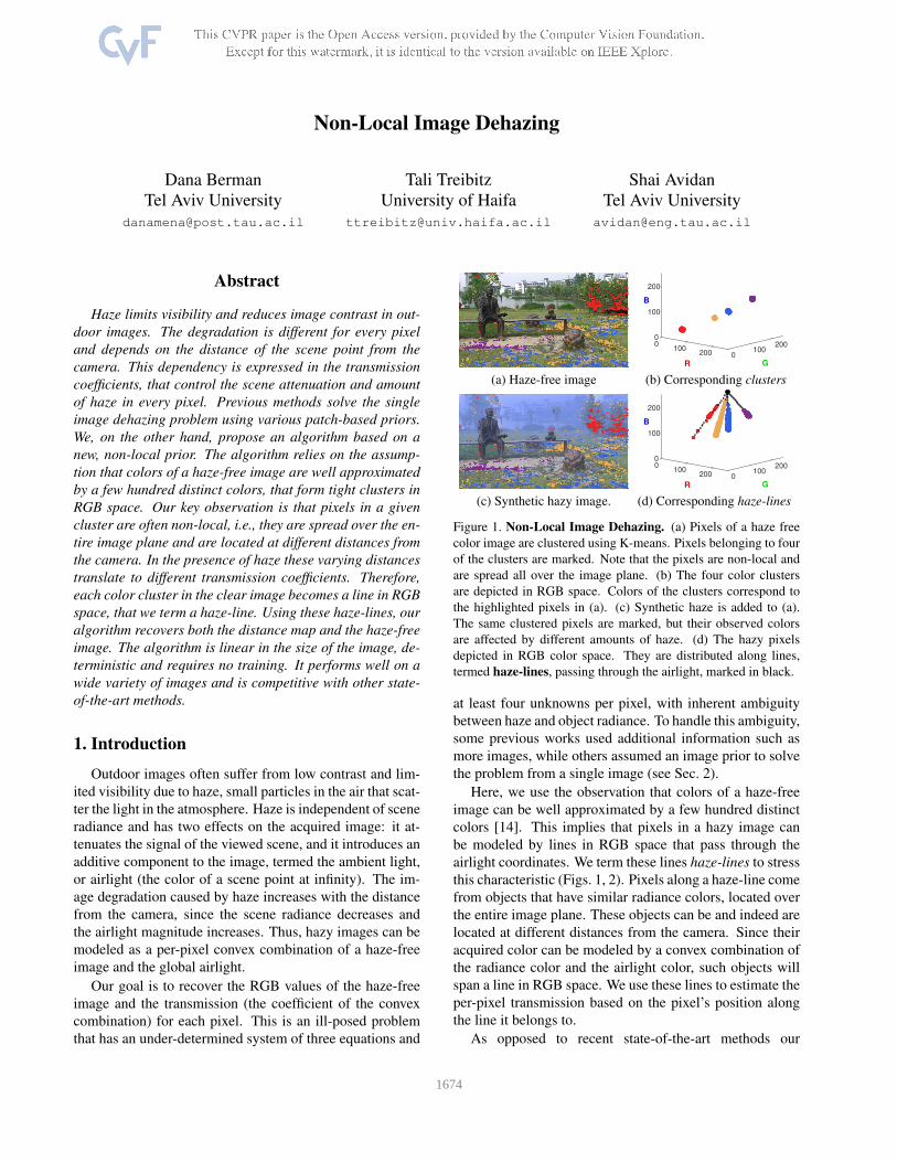
Figure 1. Non-Local Image Dehazing. (a) Pixels of a haze free
color image are clustered using K-means. Pixels belonging to four
of the clusters are marked. Note that the pixels are non-local and
are spread all over the image plane. (b) The four color clusters
are depicted in RGB space. Colors of the clusters correspond to
the highlighted pixels in (a). (c) Synthetic haze is added to (a).
The same clustered pixels are marked, but their observed colors
are affected by different amounts of haze. (d) The hazy pixels
depicted in RGB color space. They are distributed along lines,
termed haze-lines, passing through the airlight, marked in black.
at least four unknowns per pixel, with inherent ambiguity
between haze and object radiance. To handle this ambiguity,
some previous works used additional information such as
more images, while others assumed an image prior to solve
the problem from a single image (see Sec. 2).
Here, we use the observation that colors of a haze-free
image can be well approximated by a few hundred distinct
colors [14]. This implies that pixels in a hazy image can
be modeled by lines in RGB space that pass through the
airlight coordinates. We term these lines haze-lines to stress
this characteristic (Figs. 1, 2). Pixels along a haze-line come
from objects that have similar radiance colors, located over
the entire image plane. These objects can be and indeed are
located at different distances from the camera. Since their
acquired color can be modeled by a convex combination of
the radiance color and the airlight color, such objects will
span a line in RGB space. We use these lines to estimate the
per-pixel transmission based on the pixel’s position along
the line it belongs to.
As opposed to recent state-of-the-art methods our
11674

0
100
200
A
B
200
G
100 200
R
1000
0
100
200
A
B
200
G
100
(1-t)A
200
R
1000
(a) Input hazy image: Forest. (b) The circled pixels form a (c) The pixels in the orange square
Note pixels marked in circles haze-line in RGB color space form a color-line in RGB color space
Figure 2. Haze-lines (ours) vs. Color lines [3]. (a) An input hazy image. Six pixels belonging to similar objects in different distances are
marked by round color markers, and a local patch is marked by an orange frame. (b) The color coordinates of the pixels depicted in (a)
with round markers are shown in RGB color space, with a corresponding color coding. They are distributed over a haze-line, as identified
by our method. The line passes through the airlight, marked in black. The other end of the line is the haze-free color of these pixels, not
the origin. (c) As opposed to our method, the pixels in the local patch marked by an orange square are distributed along a color line [3]
that intersects the vector from the origin to the airlight.
method is global and does not divide the image to patches.
Patch-based methods take great care to avoid artifacts by
either using multiple patch sizes [19] or taking into consid-
eration patch overlap and regularization using connections
between distant pixels [3]. In our case, the pixels that form
the haze-lines are spread across the entire image and there-
fore capture a global phenomena that is not limited to small
image patches. Thus, our prior is more robust and signifi-
cantly more efficient in run-time.
We propose an efficient algorithm that is linear in the
size of the image. We automatically detect haze-lines and
use them to dehaze the image. We also conduct extensive
experiments to validate our assumptions and report quanti-
tative and qualitative results on many outdoor images.
2. Previous Work
A variety of approaches have been proposed to solve im-
age dehazing. Several methods require additional informa-
tion to dehaze images, such as multiple images taken under
different weather conditions [11], or two images with dif-
ferent polarization states [16]. Alternatively, the scene ge-
ometry is used [6]. Single image dehazing methods assume
only the input image is available and rely on image priors.
Haze reduces the contrast in the image, and various
methods rely on this observation for restoration. Tan [18]
maximizes the contrast per patch, while maintaining a
global coherent image. In [15] the amount of haze is es-
timated from the difference between the RGB channels,
which decreases as haze increases. This assumption is prob-
lematic in gray areas. In [21] the haze is estimated based on
the observation that hazy regions are characterized by high
brightness and low saturation.
Some methods use a prior on the depth of the image.
A smoothness prior on the airlight is used in [20], assum-
ing it is smooth except for depth discontinuities. Nishino
et al. [12] assume the scene albedo and depth are statisti-
cally independent and jointly estimate them using priors on
both. The prior on the albedo assumes the distribution of
gradients in images of natural scenes exhibits a heavy-tail
distribution, and it is approximated as a generalized normal
distribution. The depth prior is scene-dependent, and is cho-
sen manually, either as piece-wise constant for urban scenes
or smoothly varying for non-urban landscapes.
Several methods assume that transmission and radiance
are piece-wise constant, and employ a prior on a patch basis
[3, 4, 5]. The dark channel prior [5] assumes that within
small image patches there will be at least one pixel with a
dark color channel and use this minimal value as an estimate
of the present haze. This prior works very well, except in
bright areas of the scene where the prior does not hold.
In [4], color ellipsoids are fitted in RGB space per-patch.
These ellipsoids are used to provide a unified approach for
previous single image dehazing methods, and a new method
is proposed to estimate the transmission in each ellipsoid.
In [3, 17], color lines are fitted in RGB space per-patch,
looking for small patches with a constant transmission. This
prior is based on the observation [13] that pixels in a haze-
free image form color lines in RGB space. These lines pass
through the origin and stem from shading variations within
objects. As shown in [3], the color lines in hazy images
do not pass through the origin anymore, due to the additive
haze component. In small patches that contain pixels in a
uniform distance from the camera, these lines are shifted
from the origin by the airlight at that distance. By fitting
a line to each such patch, the transmission in the patch is
estimated using the line’s shift from the origin.
The variety of priors has led to the work of [19], that
examines different patch features in a learning framework.
Instead of small patches, in [7] the image is segmented to
regions with similar distances, and the contrast is stretched
within each segment. This may create artifacts at the bound-
aries between segments.
1675
While our haze-lines might seem similar to [3, 4], they
are inherently different. The differences are shown in Fig. 2.
In [3], lines are defined by the pixels of small patches in
the image plane assuming constant transmission, with inten-
sity differences caused by shading, and therefore relatively
small (Fig. 2c). This is a local phenomena that does not
always hold and indeed, in [3] care is taken to ensure only
patches where the assumption holds are considered. We, on
the other hand, look at lines that are formed by individual
pixels that are scattered over the entire image. These pix-
els usually have large intensity differences that are caused
by changes in transmission and not local shading effects, as
demonstrated in Fig. 2b.
3. Non-Local Colors in Hazy Images
We first present the haze model and then describe how
we use non-local haze-lines for image dehazing.
3.1. Haze Model
The common hazy image formation model is [9]:
I(x) = t(x) · J(x) + [1− t(x)] ·A , (1)
where x is the pixel coordinates, I is the observed hazy im-
age, and J is the true radiance of the scene point imaged at
x. The airlight A is a single color representing the airlight
in image areas where t = 0.
The scene transmission t(x) is distance-dependent:
t(x) = e−βd(x) , (2)
where β is the attenuation coefficient of the atmosphere and
d(x) is the distance of the scene at pixel x. Generally, β is
wavelength dependent and therefore t is different per color
channel [11, 16]. This dependency has been assumed negli-
gible in previous single image dehazing methods to reduce
the number of unknowns and we follow this assumption.
The transmission t(x) acts as a matting coefficient between
the scene J and the airlight A. Thus, per-pixel x, Eq. (1)
has three observations I(x) and four unknowns: J(x) and
t(x), resulting in an under-determined estimation problem.
3.2. The Prior
Our method is based on the observation that the number
of distinct colors in an image is orders of magnitude smaller
than the number of pixels [14]. This assumption has been
used extensively in the past and is used for saving color
images using indexed colormaps. We validate and quan-
tify it on the Berkeley Segmentation Dataset (BSDS300).
This is a diverse dataset of clear outdoor natural images and
thus represents the type of scenes that might be degraded
by haze. We clustered the RGB pixel values of each image
using K-means to a maximum of 500 clusters, and replaced
every pixel in the image with its respective cluster center.
The result is an image with 500 different RGB values at
PSNR [dB]
36 38 40 42 44 46 48 50 52 54
Pro
babili
ty
0
0.05
0.1
0.15
0.2
(a) quantization PSNR histogram (b) Before color quantization
(c) Absolute difference image (d) After color quantization
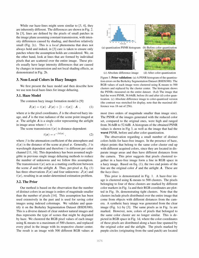
Figure 3. Prior validation: (a) A PSNR histogram of the quantiza-
tion errors on the Berkeley Segmentation Dataset (BSDS300): The
RGB values of each image were clustered using K-means to 500
clusters and replaced by the cluster center. The histogram shows
the PSNRs measured on the entire dataset. (b,d) The image that
had the worst PSNR, 36.64dB, before (b) and after (d) color quan-
tization. (c) Absolute difference image to color-quantized version
(the contrast was stretched for display, note that the maximal dif-
ference was 18 out of 256).
most (two orders of magnitude smaller than image size).
The PSNR of the images generated with the reduced color
set, compared to the original ones, were high and ranged
from 36.6dB to 52.6dB. A histogram of the obtained PSNR
values is shown in Fig 3, as well as the image that had the
worst PSNR, before and after color quantization.
The observation regarding a small number of distinct
colors holds for haze-free images. In the presence of haze,
object points that belong to the same color cluster end up
with different acquired colors, since they are located in dis-
parate image areas and thus have different distances from
the camera. This prior suggests that pixels clustered to-
gether in a haze-free image form a line in RGB space in
a hazy image. Based on Eq. (1), the two end points of the
line are the original color J and the airlight A. These are
the haze-lines.
This prior is demonstrated in Fig. 1. A haze-free im-
age is clustered using K-means to 500 clusters. The pixels
belonging to four of these clusters are marked by different
color markers in Fig. 1a and their RGB coordinates are plot-
ted in Fig. 1b, demonstrating tight clusters. Note that the
clusters include pixels distributed over the entire image that
come from objects with different distances from the cam-
era. A synthetic hazy image was generated from the clear
image (Fig. 1c) by [3]. The same pixels as in Fig. 1a are
marked. However, now, colors of pixels that belonged to
the same color cluster are no longer similar. This is de-
picted in RGB space in Fig. 1d, where the color coordinates
of these pixels are distributed along a haze-line spanned by
the original color and the airlight. The pixels marked by
purple circles (originating from the sand patch) are located
1676
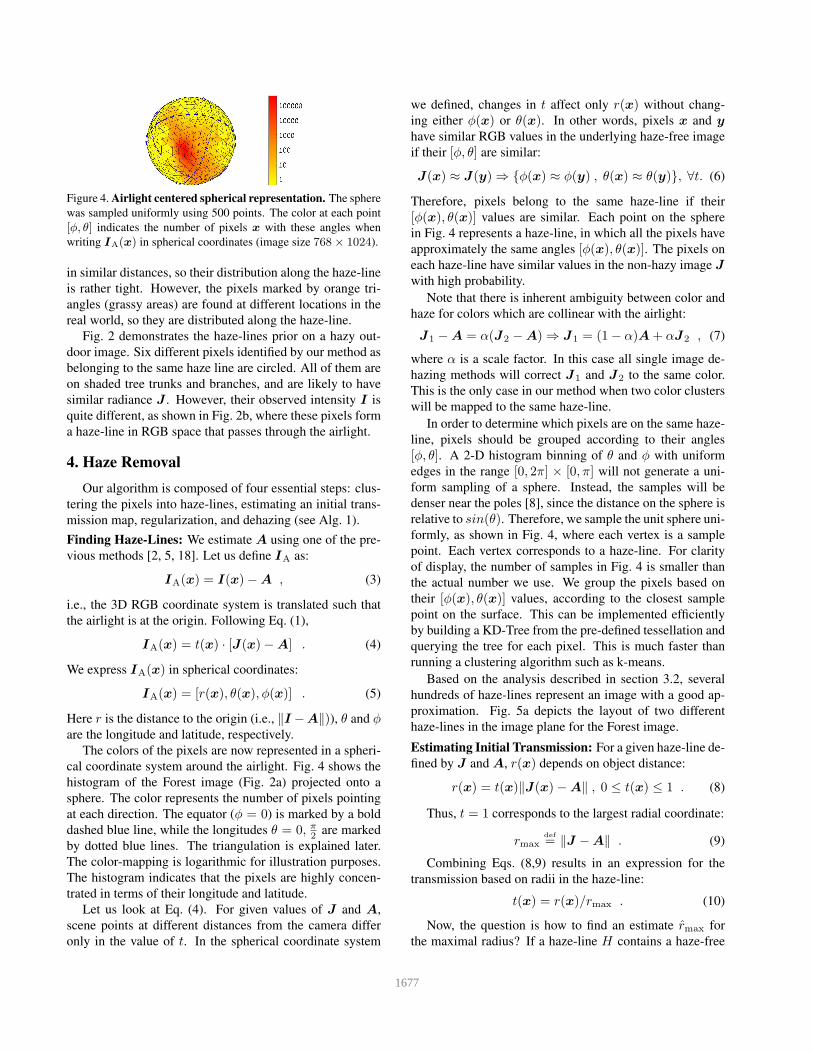
Figure 4. Airlight centered spherical representation. The sphere
was sampled uniformly using 500 points. The color at each point
[φ, θ] indicates the number of pixels x with these angles when
writing IA(x) in spherical coordinates (image size 768× 1024).
in similar distances, so their distribution along the haze-line
is rather tight. However, the pixels marked by orange tri-
angles (grassy areas) are found at different locations in the
real world, so they are distributed along the haze-line.
Fig. 2 demonstrates the haze-lines prior on a hazy out-
door image. Six different pixels identified by our method as
belonging to the same haze line are circled. All of them are
on shaded tree trunks and branches, and are likely to have
similar radiance J . However, their observed intensity I is
quite different, as shown in Fig. 2b, where these pixels form
a haze-line in RGB space that passes through the airlight.
4. Haze Removal
Our algorithm is composed of four essential steps: clus-
tering the pixels into haze-lines, estimating an initial trans-
mission map, regularization, and dehazing (see Alg. 1).
Finding Haze-Lines: We estimate A using one of the pre-
vious methods [2, 5, 18]. Let us define IA as:
IA(x) = I(x)−A , (3)
i.e., the 3D RGB coordinate system is translated such that
the airlight is at the origin. Following Eq. (1),
IA(x) = t(x) · [J(x)−A] . (4)
We express IA(x) in spherical coordinates:
IA(x) = [r(x), θ(x), φ(x)] . (5)
Here r is the distance to the origin (i.e., ‖I −A‖)), θ and φare the longitude and latitude, respectively.
The colors of the pixels are now represented in a spheri-
cal coordinate system around the airlight. Fig. 4 shows the
histogram of the Forest image (Fig. 2a) projected onto a
sphere. The color represents the number of pixels pointing
at each direction. The equator (φ = 0) is marked by a bold
dashed blue line, while the longitudes θ = 0, π2 are marked
by dotted blue lines. The triangulation is explained later.
The color-mapping is logarithmic for illustration purposes.
The histogram indicates that the pixels are highly concen-
trated in terms of their longitude and latitude.
Let us look at Eq. (4). For given values of J and A,
scene points at different distances from the camera differ
only in the value of t. In the spherical coordinate system
we defined, changes in t affect only r(x) without chang-
ing either φ(x) or θ(x). In other words, pixels x and y
have similar RGB values in the underlying haze-free image
if their [φ, θ] are similar:
J(x) ≈ J(y) ⇒ {φ(x) ≈ φ(y) , θ(x) ≈ θ(y)}, ∀t. (6)
Therefore, pixels belong to the same haze-line if their
[φ(x), θ(x)] values are similar. Each point on the sphere
in Fig. 4 represents a haze-line, in which all the pixels have
approximately the same angles [φ(x), θ(x)]. The pixels on
each haze-line have similar values in the non-hazy image J
with high probability.
Note that there is inherent ambiguity between color and
haze for colors which are collinear with the airlight:
J1 −A = α(J2 −A) ⇒ J1 = (1− α)A+ αJ2 , (7)
where α is a scale factor. In this case all single image de-
hazing methods will correct J1 and J2 to the same color.
This is the only case in our method when two color clusters
will be mapped to the same haze-line.
In order to determine which pixels are on the same haze-
line, pixels should be grouped according to their angles
[φ, θ]. A 2-D histogram binning of θ and φ with uniform
edges in the range [0, 2π] × [0, π] will not generate a uni-
form sampling of a sphere. Instead, the samples will be
denser near the poles [8], since the distance on the sphere is
relative to sin(θ). Therefore, we sample the unit sphere uni-
formly, as shown in Fig. 4, where each vertex is a sample
point. Each vertex corresponds to a haze-line. For clarity
of display, the number of samples in Fig. 4 is smaller than
the actual number we use. We group the pixels based on
their [φ(x), θ(x)] values, according to the closest sample
point on the surface. This can be implemented efficiently
by building a KD-Tree from the pre-defined tessellation and
querying the tree for each pixel. This is much faster than
running a clustering algorithm such as k-means.
Based on the analysis described in section 3.2, several
hundreds of haze-lines represent an image with a good ap-
proximation. Fig. 5a depicts the layout of two different
haze-lines in the image plane for the Forest image.
Estimating Initial Transmission: For a given haze-line de-
fined by J and A, r(x) depends on object distance:
r(x) = t(x)‖J(x)−A‖ , 0 ≤ t(x) ≤ 1 . (8)
Thus, t = 1 corresponds to the largest radial coordinate:
rmaxdef
= ‖J −A‖ . (9)
Combining Eqs. (8,9) results in an expression for the
transmission based on radii in the haze-line:
t(x) = r(x)/rmax . (10)
Now, the question is how to find an estimate rmax for
the maximal radius? If a haze-line H contains a haze-free
1677

Figure 5. Distance distribution per haze-line: (a) Pixels belong-
ing to two different haze-lines are depicted in green and blue, re-
spectively. (b) A histogram of r(x) within each cluster. The hori-
zontal axis is limited to the range [0, ‖A‖], as no pixel can have a
radius outside that range in this particular image.
pixel, then rmax is the maximal radius of that haze-line:
rmax(x) = maxx∈H
{r(x)} , (11)
where the estimation is done per haze-line H . Fig. 5b
displays the radii histograms of the two clusters shown in
Fig. 5a. We assume that the farthest pixel from the airlight
is haze free, and that such a pixel exists for every haze-line.
This assumption does not hold for all of the haze-lines in an
image, however the regularization step partially compen-
sates for it. Combining Eqs. (10,11) results in a per-pixel
estimation of the transmission:
t(x) = r(x)/rmax(x) . (12)
Regularization: Since the radiance J is positive (i.e.,
J ≥ 0 ), Eq. (1) gives a lower bound on the transmission:
tLB(x) = 1− minc∈{R,G,B}
{Ic(x)/Ac} . (13)
In [5], the transmission estimate is based on an eroded
version of tLB . We impose this bound on the estimated
transmission, per-pixel:
tLB(x) = max{t(x), tLB(x)} . (14)
The estimation in Eq. (12) is performed per-pixel, with-
out imposing spatial coherency. This estimation can be
inaccurate if a small amount of pixels were mapped to a
particular haze-line, or in very hazy areas, where r(x) is
very small and noise can affect the angles significantly. The
transmission map should be smooth, except for depth dis-
continuities [3, 12, 18, 20]. We seek a transmission map
t(x) that is similar to tLB(x) and is smooth when the input
image is smooth. Mathematically, we minimize the follow-
ing function w.r.t. t(x):
∑
x
[
t(x)− tLB(x)]2
σ2(x)+ λ
∑
x
∑
y∈Nx
[
t(x)− t(y)]2
‖I(x)− I(y)‖2,
(15)
where λ is a parameter that controls trade-off between the
data and the smoothness terms, Nx denotes the four nearest
neighbors of x in the image plane and σ(x) is the standard
deviation of tLB , which is calculated per haze-line.
Algorithm 1 Haze Removal
Input: I(x),AOutput: J(x), t(x)
1: IA(x) = I(x)−A
2: Convert IA to spherical coordinates to obtain
[r(x), φ(x), θ(x)]3: Cluster the pixels according to [φ(x), θ(x)].
Each cluster H is a haze-line.
4: for each cluster H do
5: Estimate maximum radius:
rmax(x) = maxx∈H{r(x)}
6: for each pixel x do
7: Estimate transmission: t(x) = r(x)rmax
8: Perform regularization by calculating t(x) that
minimizes Eq. 15
9: Calculate the dehazed image using Eq. (16)
σ(x) plays a significant role since it allows us to ap-
ply our estimate only to pixels where the assumptions hold.
When the variance is high, the initial estimation is less reli-
able. σ(x) increases as the number of pixels in a haze line
decreases. When the radii distribution in a given haze-line
is small, our haze-line assumption does not hold since we
do not observe pixels with different amounts of haze. In
such cases, σ(x) increases as well.
Dehazing: Once t(x) is calculated as the minimum of
Eq. (15), the dehazed image is calculated using Eq. (1):
J(x) ={
I(x)−[
1− t(x)]
A}/
t(x) . (16)
The method is summarized in Alg. 1 and demonstrated
in Fig. 6. Fig. 6a shows the input hazy image. The final,
dehazed image is shown in Fig. 6b. Fig. 6c shows the dis-
tance in RGB space of every pixel in the hazy image to the
airlight. Note that this distance decreases as haze increases.
Fig. 6d shows the maximum radii rmax(x) per haze-line.
Observe that Fig. 6d is much brighter than Fig. 6c. Since
larger values are represented by brighter colors, this indi-
cates that the distance to the airlight is increased. The pixels
with the maximum radius in their haze-line are marked on
the hazy image in Fig. 6e. Note that these pixels are mostly
at the foreground, where indeed there is a minimal amount
of haze. We filtered out pixels that had a maximum radius in
the haze line, yet had a σ > 2, since the model assumptions
do not hold for these haze lines. The aforementioned pixels
are found in the sky, since the distance to the airlight in RGB
space is very short. Therefore, clustering them according to
their angles is not reliable due to noise. In the regularization
step this fact is taken into consideration through the data-
term weight 1σ2(x) , which is shown in Fig. 6f (warm colors
depict high values). The ratio of Figs. 6c and 6d yields the
initial transmission t(x) that is shown in Fig. 6g. The trans-
1678

(a) Hazy image I(x) (b) Dehazed image J(x)
(c) r(x) (d) rmax(x)
(e) pixels {x|r(x) = rmax(x)} (f) 1σ2(x)
, colomapped
(g) Initial trans. t(x) (h) Regularized trans. t(x)
Figure 6. Intermediate and final results of our method: (a) An
input hazy image; (b) The output image; (c) The distance r(x) of
every pixel of the hazy image to the airlight; (d) the estimated radii
rmax(x) calculated according to Eq. (11); (e) The input image is
shown, with the pixels x for which r(x) = rmax(x) marked by
cyan circles; (f) The data term confidence in Eq. (15) colormapped
(warm colors show the larger values); (g) The estimated transmis-
sion map t(x) before the regularization; (h) The final transmission
map t(x) after regularization. (g) and (h) are colormapped.
mission map after regularization is shown in Fig. 6h. While
t(x) contains fine details even in grass areas that are at the
same distance from the camera, t(x) does not exhibit this
behavior. This indicates the regularization is necessary.
5. Results
We evaluate our method on a large dataset containing
both natural and synthetic images and compare our perfor-
mance to state-of-the-art algorithms. We assume A is given,
by using the airlight vector A calculated by [17]. We use
the same parameters for all of the images: in Eq. (15) we
set λ = 0.1 and we scale 1/σ2(x) to be in the range [0, 1]in order to avoid numeric issues. In order to find the haze
lines, we sample uniformly 1000 points on the unit sphere
(Fig. 4 shows only 500 for clarity).
5.1. Quantitative results
A synthetic dataset of hazy images of natural scenes
was introduced by [3], and is available online. The dataset
contains eleven haze free images, synthetic distance maps
Table 1. Comparison of L1 errors over synthetic hazy images with
various amount of noise. The noise standard deviation is given and
the images are scaled to the range [0, 1]. The table compares the
L1 errors of the estimated transmission maps (left value) and the
dehazed images (right value).σ [5] [3] ours
Road1
0 0.097/ 0.051 0.069/ 0.033 0.058/ 0.040
0.01 0.100/ 0.058 0.068/ 0.038 0.061/ 0.045
0.025 0.106/ 0.074 0.084/ 0.065 0.072/ 0.064
0.05 0.136/ 0.107 0.120/ 0.114 0.091/ 0.100
Lawn1
0 0.118/ 0.063 0.077/ 0.035 0.032/ 0.026
0.01 0.116/ 0.067 0.056/ 0.038 0.032/ 0.032
0.025 0.109/ 0.077 0.056/ 0.065 0.052/ 0.056
0.05 0.115/ 0.102 0.114/ 0.121 0.099/ 0.107
Mansion
0 0.074/ 0.043 0.042/ 0.022 0.080/ 0.049
0.01 0.067/ 0.040 0.048/ 0.030 0.088/ 0.056
0.025 0.057/ 0.044 0.065/ 0.051 0.104/ 0.072
0.05 0.083/ 0.075 0.081/ 0.080 0.116/ 0.095
Church
0 0.07/ 0.048 0.039/ 0.025 0.047/ 0.032
0.01 0.067/ 0.050 0.053/ 0.043 0.049/ 0.041
0.025 0.058/ 0.059 0.089/ 0.081 0.047/ 0.057
0.05 0.087/ 0.121 0.121/ 0.136 0.043/ 0.092
Raindeer
0 0.127/ 0.068 0.066/ 0.034 0.089/ 0.045
0.01 0.119/ 0.066 0.077/ 0.042 0.093/ 0.049
0.025 0.109/ 0.067 0.084/ 0.054 0.104/ 0.063
0.05 0.117/ 0.085 0.106/ 0.083 0.131/ 0.092
and corresponding simulated haze images. An identically-
distributed zero-mean Gaussian noise with three different
noise level: σn = 0.01, 0.025, 0.05 was added to these im-
ages (with image intensity scaled to [0, 1]). Table 1 sum-
marizes the L1 errors on non-sky pixels (same metric used
in [3]) of the transmission maps and the dehazed images.
Our method is compared to the method of [3] and an imple-
mentation of [5] by [3]. For five images out of this dataset,
results of both clear and noisy images are provided by [3]1.
Our method outperforms previous methods in most
cases, and handles the noise well. As expected, our perfor-
mance degrades when the noise variance increases. How-
ever, our method maintains its ranking, with respect to other
methods, regardless of the amount of noise. This shows that
our algorithm is quite robust to noise, despite being pixel-
based.
5.2. Qualitative results
Figs. 7 and 8 compare our results to state-of-the-art sin-
gle image dehazing methods [1, 3, 4, 5, 12, 19]. As previ-
ously noted by [5], the image after haze removal might look
dim, since the scene radiance is usually not as bright as the
airlight. For display, we perform a global linear contrast
stretch on the output, clipping 0.5% of the pixel values both
in the shadows and in the highlights. Pixels whose radius is
maximal in their haze-line are marked in pink on the hazy
input. We marked only pixels x for which σ(x) < 2 and
for clarity, only ones that belong to large clusters.
1A complete summary of results and more is available on the project’s
website.
1679

hazy image: House He et al. [5] Gibson and Nguyen [4] Nishino et al. [12] Fattal [3] Ours
hazy image: Train He et al. [5] Luzon-Gonzalez et al. [7] Ancuti and Ancuti [1] Fattal [3] Ours
hazy image: Cityscape He et al. [5] Gibson and Nguyen [4] Tang et al. [19] Fattal [3] Ours
Figure 7. Comparison on natural images: [Left] Input with pixels that set the maximum radius in their haze-line circled in pink.
[Right] Our result. Middle columns display results by several methods, since each paper reports results on a different set of images.
Top to bottom:
hazy image: Forest
He et al. [5] results
Fattal [3] results
our results
Figure 8. Comparison of transmission maps and dehazed images.
The method of [1] leaves haze in the results, as seen in
the areas circled in yellow in Fig. 7. In the result of [7] there
are artifacts in the boundary between segments (pointed by
arrows). The method of [12] tends to oversaturate (e.g.,
House). The methods of [5, 19] produce excellent results in
general but lack some micro-contrast when compared to [3]
and to ours. This is evident in the zoomed-in buildings
shown in Cityscape results, where in our result and in [3]
the windows are sharper than in [5, 19] (best viewed on a
monitor). The result of [4] was not enlarged as it has a low
resolution. Results of [3] are sometimes clipped, e.g., the
leaves in House and in the sky in Forest.
Our assumption regarding having a haze-free pixel in
each haze-line does not hold in Cityscape, as evident by
several hazy pixels that set a maximum radius, e.g. the red
buildings. Despite that, the transmission in those areas is
estimated correctly due to the regularization that propagates
the depth information spatially from the other haze-lines.
Fig. 8 compares both the transmission maps and the de-
hazed images. It shows our method is comparable to other
methods, and in certain cases works better. For example,
The two rows of trees are well separated in our result when
compared to [5].
The main advantage of the global approach is the ability
to cope well with fast variations in depth, when the details
are smaller than the patch size. Fig. 9 shows an enlarged
1680
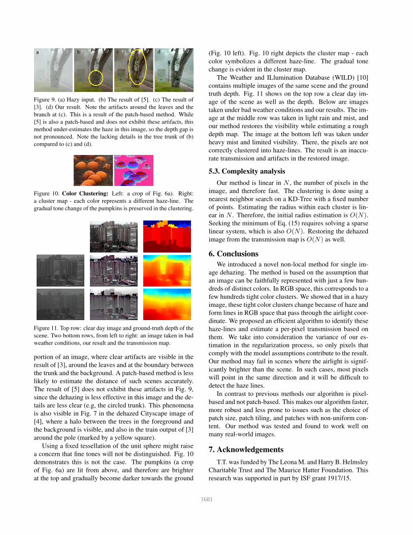
Figure 9. (a) Hazy input. (b) The result of [5]. (c) The result of
[3]. (d) Our result. Note the artifacts around the leaves and the
branch at (c). This is a result of the patch-based method. While
[5] is also a patch-based and does not exhibit these artifacts, this
method under-estimates the haze in this image, so the depth gap is
not pronounced. Note the lacking details in the tree trunk of (b)
compared to (c) and (d).
Figure 10. Color Clustering: Left: a crop of Fig. 6a). Right:
a cluster map - each color represents a different haze-line. The
gradual tone change of the pumpkins is preserved in the clustering.
Figure 11. Top row: clear day image and ground-truth depth of the
scene. Two bottom rows, from left to right: an image taken in bad
weather conditions, our result and the transmission map.
portion of an image, where clear artifacts are visible in the
result of [3], around the leaves and at the boundary between
the trunk and the background. A patch-based method is less
likely to estimate the distance of such scenes accurately.
The result of [5] does not exhibit these artifacts in Fig. 9,
since the dehazing is less effective in this image and the de-
tails are less clear (e.g, the circled trunk). This phenomena
is also visible in Fig. 7 in the dehazed Cityscape image of
[4], where a halo between the trees in the foreground and
the background is visible, and also in the train output of [3]
around the pole (marked by a yellow square).
Using a fixed tessellation of the unit sphere might raise
a concern that fine tones will not be distinguished. Fig. 10
demonstrates this is not the case. The pumpkins (a crop
of Fig. 6a) are lit from above, and therefore are brighter
at the top and gradually become darker towards the ground
(Fig. 10 left). Fig. 10 right depicts the cluster map - each
color symbolizes a different haze-line. The gradual tone
change is evident in the cluster map.
The Weather and ILlumination Database (WILD) [10]
contains multiple images of the same scene and the ground
truth depth. Fig. 11 shows on the top row a clear day im-
age of the scene as well as the depth. Below are images
taken under bad weather conditions and our results. The im-
age at the middle row was taken in light rain and mist, and
our method restores the visibility while estimating a rough
depth map. The image at the bottom left was taken under
heavy mist and limited visibility. There, the pixels are not
correctly clustered into haze-lines. The result is an inaccu-
rate transmission and artifacts in the restored image.
5.3. Complexity analysis
Our method is linear in N , the number of pixels in the
image, and therefore fast. The clustering is done using a
nearest neighbor search on a KD-Tree with a fixed number
of points. Estimating the radius within each cluster is lin-
ear in N . Therefore, the initial radius estimation is O(N).Seeking the minimum of Eq. (15) requires solving a sparse
linear system, which is also O(N). Restoring the dehazed
image from the transmission map is O(N) as well.
6. Conclusions
We introduced a novel non-local method for single im-
age dehazing. The method is based on the assumption that
an image can be faithfully represented with just a few hun-
dreds of distinct colors. In RGB space, this corresponds to a
few hundreds tight color clusters. We showed that in a hazy
image, these tight color clusters change because of haze and
form lines in RGB space that pass through the airlight coor-
dinate. We proposed an efficient algorithm to identify these
haze-lines and estimate a per-pixel transmission based on
them. We take into consideration the variance of our es-
timation in the regularization process, so only pixels that
comply with the model assumptions contribute to the result.
Our method may fail in scenes where the airlight is signif-
icantly brighter than the scene. In such cases, most pixels
will point in the same direction and it will be difficult to
detect the haze lines.
In contrast to previous methods our algorithm is pixel-
based and not patch-based. This makes our algorithm faster,
more robust and less prone to issues such as the choice of
patch size, patch tiling, and patches with non-uniform con-
tent. Our method was tested and found to work well on
many real-world images.
7. Acknowledgements
T.T. was funded by The Leona M. and Harry B. Helmsley
Charitable Trust and The Maurice Hatter Foundation. This
research was supported in part by ISF grant 1917/15.
1681
References
[1] C. O. Ancuti and C. Ancuti. Single image dehazing by multi-
scale fusion. IEEE Trans. on Image Processing, 22(8):3271–
3282, 2013.
[2] R. Fattal. Single image dehazing. ACM Trans. Graph.,
27(3):72, 2008.
[3] R. Fattal. Dehazing using color-lines. ACM Trans. Graph.,
34(1):13, 2014.
[4] K. B. Gibson and T. Q. Nguyen. An analysis of single im-
age defogging methods using a color ellipsoid framework.
EURASIP Journal on Image and Video Processing, 2013(1),
2013.
[5] K. He, J. Sun, and X. Tang. Single image haze removal using
dark channel prior. In Proc. IEEE CVPR, 2009.
[6] J. Kopf, B. Neubert, B. Chen, M. Cohen, D. Cohen-Or,
O. Deussen, M. Uyttendaele, and D. Lischinski. Deep photo:
Model-based photograph enhancement and viewing. ACM
Trans. Graph., 27(5):116, 2008.
[7] R. Luzon-Gonzalez, J. L. Nieves, and J. Romero. Recovering
of weather degraded images based on RGB response ratio
constancy. Appl. Opt., 2014.
[8] G. Marsaglia. Choosing a point from the surface of a sphere.
Ann. Math. Statist., 43(2):645–646, 04 1972.
[9] W. E. K. Middleton. Vision through the atmosphere. Toronto:
University of Toronto Press, 1952.
[10] S. Narasimhan, C. Wang, and S. Nayar. All the Images of
an Outdoor Scene. In European Conference on Computer
Vision (ECCV), volume III, pages 148–162, May 2002.
[11] S. G. Narasimhan and S. K. Nayar. Chromatic framework
for vision in bad weather. In Proc. IEEE CVPR, 2000.
[12] K. Nishino, L. Kratz, and S. Lombardi. Bayesian defog-
ging. Int. Journal of Computer Vision (IJCV), 98(3):263–
278, 2012.
[13] I. Omer and M. Werman. Color lines: Image specific color
representation. In Proc. IEEE CVPR, 2004.
[14] M. T. Orchard and C. A. Bouman. Color quantization
of images. Signal Processing, IEEE Transactions on,
39(12):2677–2690, 1991.
[15] D. Park, D. K. Han, C. Jeon, and H. Ko. Fast single image de-
hazing using characteristics of RGB channel of foggy image.
IEICE Trans. on Information and Systems, 96(8):1793–1799,
2013.
[16] Y. Y. Schechner, S. G. Narasimhan, and S. K. Nayar. Instant
dehazing of images using polarization. In Proc. IEEE CVPR,
2001.
[17] M. Sulami, I. Geltzer, R. Fattal, and M. Werman. Automatic
recovery of the atmospheric light in hazy images. In Proc.
IEEE ICCP, 2014.
[18] R. Tan. Visibility in bad weather from a single image. In
Proc. IEEE CVPR, 2008.
[19] K. Tang, J. Yang, and J. Wang. Investigating haze-relevant
features in a learning framework for image dehazing. In
Proc. IEEE CVPR, 2014.
[20] J.-P. Tarel and N. Hautiere. Fast visibility restoration from a
single color or gray level image. In Computer Vision, 2009
IEEE 12th International Conference on, pages 2201–2208,
Sept 2009.
[21] Q. Zhu, J. Mai, and L. Shao. Single image dehazing using
color attenuation prior. In Proc. British Machine Vision Con-
ference (BMVC), 2014.
1682