Non-Cartesian Reconstruction

John Pauly

October 17, 2005

1 Introduction

There are many alternatives to spin-warp, or2DFT, acquisition methods. These include spi-ral scans, radial scans, variations of echo-planar,and many other less common acquisitions (rosette,Lissajou, ...). All of these are relatively easyto program on modern commercial imaging sys-tems. Many of these have specific advantages overspin-warp, such as speed, flow performance, andSNR efficiency. The main disadvantage with thesemethods is the difficulty of reconstructing the re-sulting data sets. This chapter concerns methodsfor reconstructing these data sets that do not fallon a regular Cartesian grid in spatial-frequencyspace. This is a very important topic. Once thereconstruction limitations are removed, there aremany more options for collecting MRI data.

One of the most important advantages of spin-warp, is that the reconstruction can be performedwith a simple 2D DFT. This is easily implemented,and very efficient. For non-Cartesian data setsthere are many options. The first approach is tocollect the non-Cartesian data in a way that a pre-viously known reconstruction method, like projec-tion reconstruction, can be applied. While thissolves the reconstruction problem, it usually re-quires compromises in data acquisition. Second,the non-Cartesian data can be demodulated point-by-point with the conjugate phase reconstruction.This works, but is slow. Better approaches in-volve first resampling the data to a Cartesian grid,and then using a 2DFT for the reconstruction.

kx

ky

t

GyGxa) b)

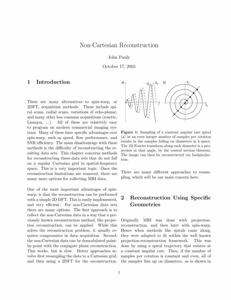
Figure 1: Sampling of a constant angular rate spiral(a) at an even integer number of samples per rotationresults in the samples falling on diameters in k-space.The 1D Fourier transform along each diameter is a pro-jection at that angle, by the central section theorem.The image can then be reconstructed via backprojec-tion.

There are many different approaches to resam-pling, which will be our main concern here.

2 Reconstruction Using SpecificGeometries

Originally MRI was done with projection-reconstruction, and then later with spin-warp.Hence when methods like spirals came along,they were adapted to fit within the well knownprojection-reconstruction framework. This wasdone by using a spiral trajectory that rotates ata constant angular rate. Then, if the number ofsamples per rotation is constant and even, all ofthe samples line up on diameters, as is shown in

1

Fig. 1. The data along a diameter is the transformof a projection, by the central section theorem.Hence, a full set of projections can be computed,and the image reconstructed using backprojection,as in X-ray CT. The drawback of this approach isthat a constant angular rate spiral does not makeefficient use of the gradient system performance,and typically results in acquisitions that are

√2

longer than would be required for a constant slewrate spiral.

Another example where an acquisition is fit into aspecific geometry for reconstruction is echo-planarimaging. In conventional EPI, the slow phaseencode axis is applied continuously as the fastaxis oscillates. The result is a sinusoidal trajec-tory through k-space. For reconstruction conve-nience it is assumed the trajectory actually fol-lows a raster scan, which results in ghosting arti-facts from objects with high spatial frequencies inx. To improve this, blipped EPI uses a blippedphase-encode gradient, so that the kx–ky trajec-tory is in fact a raster scan. However, this stillleaves problems with off-resonance, which has tofollow the conventional EPI trajectory, since off-resonance precession happens continuously. A po-tentially better alternative is to use a conventionalEPI trajectory, where y and the off-resonance fre-quency ω are indistinguishable, and reconstructusing the true non-Cartesian reconstruction trajec-tory. Then off-resonance produces only geometricdistortion, without ghosting.

3 Sensitive Point and ConjugatePhase Reconstruction

Some of the early imaging methods could not eas-ily be fit into the framework of known reconstruc-tion methods. One of the earliest methods for MRIimaging was called “sensitive point.”The basic ideawas to continuously vary the gradients in three di-mensions. The point at the isocenter of the gra-

kx

ky

Figure 2: Lissajou k-space trajectory.

dients sees no change, and continues to producea constant signal thoughout the experiment. Allother points see some time-varying field. If thegradient waveforms are properly chosen, the sig-nal from these other points will integrate to zero,while the signal at the origin will integrate coher-ently to a value proportional to the magnetizationthere. In the original implementation, the subjectwas translated in the magnet to move a new voxelto isocenter, and the process repeated.

For sensitive point imaging, the sinusoidal gradi-ents are applied. In multiple dimensions the fre-quencies of the sinusoids are chosen to be relativelyprime. Otherwise the trajectory can retrace itself,and not all of k-space will be covered with the de-sired density. A sample Lissajou pattern k-spacetrajectory is shown in Fig. 2

The k-space trajectory is

kx(t) = kmax sin(2πΩxt/T ) (1)ky(t) = kmax sin(2πΩyt/T ) (2)

where Ωx is 19, and Ωy is 20 in this case. Thegradient waveforms that produce this trajectoryare

Gx(t) =kmaxT

(2π)2γΩxcos(2πΩxt/T ) (3)

2

Slice Selection

Data Encoding andAcquisition

R F

G z

G y

G x

Figure 3: Pulse sequence that generates a Lissijou k-space trajectory.

Gy(t) =kmaxT

(2π)2γΩycos(2πΩyt/T ) (4)

These waveforms are plotted in the pulse sequenceshown in Fig. 3.

The interesting thing about sensitive point is thatit was one of the first imaging methods that didn’tfall under one of the previously known reconstruc-tion methods. The samples don’t fall on a recti-linear grid, so a simple 2DFT is inadequate for re-construction. The samples also don’t fall on radiallines, so projection-reconstruction can’t be used.This required a new perspective on reconstruction.

The new idea was to demodulate the signal foreach individual output voxel. Effectively the re-ceiver is made to track the phase of a particularvoxel so that its signal coherently adds over theduration of the acquisition. Ideally, the signal fromother voxels do not add coherently, and integrateto zero. By selectively tuning to one voxel afteranother, an image can be built up. And, since thedemodulation can be performed in software afterthe data is acquired, a single acquisition can beused to resolve all of the voxels in an image bypostprocessing.

3.1 Conjugate Phase Reconstruction

The method developed to reconstruct sensitivepoint data was called a conjugate phase reconstruc-tion. From Chapter 1, the signal from an acquisi-tion is

s(t) =∫X

Mxy(x)e−i2πk(t)·xdx. (5)

For a conjugate phase reconstruction of the signalat some point x0 we take this acquired signal andmultiply it by the conjugate of the phase at thepoint throughout the acquisition, and then inte-grate over the duration of the acquisition,

m(x0) =∫ T

0s(t)ei2πk(t)·x0dt. (6)

If we substitute for s(t) and change the order ofintegration,

m(x0) =∫X

Mxy(x)

(∫ T

0e−i2πk(t)·(x−x0)dt

)dx.

(7)This is the spatial convolution of Mxy(x) with theintegral in parentheses. At x = x0 this clearly doesthe right thing. The inner integral becomes theintegration time T , and the image value m(x0) issimply TMxy(x0). At other values of x the resultsare less clear, and depend on the characteristicsof the particular k-space trajectory. In fact, theinner integral is the impulse response of an imagingsystem using that particular k-space trajectory,

A(x) =∫ T

0e−i2πk(t)·xdt. (8)

The goal is that the impulse perform as a deltafunction, sifting out only the value of the imageat x0. Interestingly, this does not work well forLissajou trajectories, which leads to the next de-velopment in image reconstruction.

3.2 Density Correction

The problem with a Lissajou pattern can be im-mediately appreciated by examining Fig. 2. That

3

-kmax kmax0

a) Density

b) Impulse Response

x

kx

Figure 4: Sampling density of a Lissajou trajectory(a), and the impulse response that results from thisdensity (b).

is, the pattern is not at all uniform. The sam-pling density is much higher at the edges than inthe middle. The result is an impulse response that“rings” significantly, and does not do a very goodjob of localization. This is illustrated in Fig. 4.This led to the realization that conjugate phasereconstruction by itself was inadequate, and thatsome weighting must be included to account forthe sampling density.

For convenience we will just concern ourselves withthe x axis for the time being. The impulse responseis

A(x) =∫ T

0e−i2πkx(t)xdt (9)

wherekx(t) = kx,max sin(2πΩxt/T ) (10)

If the time T is an integer number of cycles at Ωx,

A(x) =∫ T

0e−i2πxkx,max sin(2πΩt/T )dt (11)

is the one dimensional projection of a two dimen-sional delta ring. The impulse response is then

A(x) = J0(πx

∆x) (12)

which is not a particularly good localization func-tion.

The reason can be seen by rewriting the expressionfor the impulse response as an integral in kx. If welook at one half cycle of the sinusoid, say from 3π/2to 5π/2, and change variables so that

dkx =∣∣∣∣dkx

dt

∣∣∣∣ dt = |γGx(t)| dt, (13)

A(x) =∫ 5π/2

3π/2e−i2πkx(t)xdt (14)

=∫ kmax

−kmax

e−i2πkxx

|γGx(t(kx))|dkx. (15)

The problem is that Gx(t) goes to zero at kx =±kmax, resulting in impulses in the k-space weight-ing. In order to make the impulse response behave,it is necessary to add an additional weighting fac-tor

W (t) = |Gx(t)| (16)

so that

A(x) =∫ T

0W (t)e−i2πk(t)·xdt. (17)

This produces the desired impulse for an impulseresponse.

The conjugate phase reconstruction is then

m(x0) =∫ T

0s(t)W (t)ei2πk(t)·x0dt. (18)

This is a solution to the problem. Unfortunately itis very slow to compute. If the image size is N×Npixels, there are on the order of N2 data samples inthe acquisition. The reconstruction of each pointrequires an N2 element inner product, and thismust be repeated for each of the N2 pixels, requir-ing on the order of N4 operations for a reconstruc-tion. The next step is to look for approaches thatperform the same functions, but more efficiently.

4

4 k-Space Resampling Methods:Overview

A much faster approach is to resample the k-spacedata onto a 2D Cartesian grid first, and then usea 2D DFT to reconstruct the image. There aremany options for resampling algorithms. Thesewill be grouped into three broad areas. The first is“ grid driven” interpolation. Here the value at eachgrid point is interpolated from the neighboring k-space data. The second is “data driven” interpola-tion, where the contribution from each data pointis added to the adjacent grid points. This includesthe gridding algorithm that we will be examiningin detail. Finally, there are a number of approachesthat try to compute local approximations to opti-mum interpolators for the specific locations of thesample points and grid points.

4.1 Grid-Driven Interpolation

The idea of grid-driven interpolation is to estimatethe value at each grid point based on the immedi-ately surrounding data. An example is illustratedin Fig. 5

One advantage of this approach is that it is easy toimplement if the location of the neighboring datapoints can be determined analytically. One exam-ple is projection-reconstruction. For other trajec-tories the locations of the neighboring data pointscan be found in a initialization stage.

It does have the disadvantage that it won’t in gen-eral use all of the input data, and hence won’t beas SNR efficient as some of the other approacheswe will consider. This isn’t as much of a drawbackas it might appear, though, because the unused ex-cess data is usually at low spatial frequencies wherethe SNR is already high, and the eye is relativelyinsensitive to errors in low spatial frequencies. Be-cause it doesn’t use all the data, this approach

kx

ky

Figure 5: Grid-driven interpolation for a projectiondata set. Data samples lie on diameters in k-space. Inthis example the surrounding four data samples (o’s)are located for each grid point (+’s), and a value at thegrid point determined by bilinear interpolation.

doesn’t require a density estimate, which can be asignificant advantage.

The fidelity of image reconstructions using this ap-proach are a tradeoff between interpolator com-plexity and k-space oversampling. If a simple bi-linear interpolator is used, image quality is poor ifthe k-space grid is the same as sampling densityrequired to support the desired image FOV. Thisis called a “1X” grid. However, if the k-space gridis twice as finely sampled, a “2X” grid, the recon-structions are quite acceptable. Sampling artifactsare below the noise floor for typical MRI images.Alternately, the use of a higher-fidelity interpola-tor could be used with a 1X grid, at the cost ofsome complexity.

In practice, this approach is seldom if ever used.Mostly this is due to the general convergence ofthe MRI community on the data-driven interpola-tion method called gridding, which we will discussnext. However, grid-driven interpolation is a rea-sonable alternative that can produce high-fidelity

5

kx

ky

Figure 6: Data-driven interpolation for a projectiondata set. Again, data samples lie on diameters in k-space. Each data point is conceptually considered tobe convolved with a small kernel, and the value of thatconvolution added to the adjacent k-space grid points.

reconstructions. This is particularly true when thesampling density is varying, such as undersampledPR, difficult to compute, or continually changing.

4.2 Data-Driven Interpolation

The idea of data-driven interpolation is to takeeach data point, and add its contribution to thesurrounding grid points. There are a number ofways this can be done. We consider here the casewhere each data point is handled uniformly. Thenext section on optimum interpolators concernsthe case where each data point is considered specif-ically as a special case.

Each input sample is conceptually considered to beconvolved with a small kernel, which is chosen tobe wide enough to extend to the neighboring gridpoints. In this way, each data point is “resampled”at the adjacent grid points. This approach hasthe advantage that all of the data is used, so it is

more SNR efficient than the grid-driven approachdescribed above. However, as a result, it needs adensity estimate to correct for the fact that thesamples may be concentrated in particular areasof k-space.

As for the grid-driven approach, reconstruction fi-delity is a tradeoff between interpolator complex-ity and k-space oversampling. Using a large kernel(e.g. 4 sample radius) on a 1X grid produces ahigh-fidelity reconstruction. Usually a good trade-off is a simpler kernel on a 2X grid, where thek-space oversampling allows for a faster interpola-tion. We will examine this in more detail below.

4.3 “Optimum” Interpolators

The data-driven interpolators use the same convo-lution kernel for each k-space sample. Better per-formance can be achieved if each data sample isconsidered independently, and has its own uniqueinterpolation function. This is typically computedover a local neighborhood to keep the computationwithin reason, so it is only an approximation to theoptimum interpolators. The computation of thesefunctions for each data sample requires a signifi-cant amount of setup time. However, once thesehave been computed they can be used repeatedly.The main advantage of this approach is the abil-ity to produce high fidelity reconstructions on a1X grid. There are two examples we will examine.One is called BURS, and the other is the nuFFTalgorithm that has been increasingly of interest.

5 Gridding Reconstruction

The reconstruction method that we will considerin the greatest detail is called gridding. After in-troducing the basic idea, we will examine the threemain design concerns in implementing a griddingreconstruction. These are the choice of a convolu-

6

Cartesian Grid

k-Space Trajectory

Convolution Kernel

Figure 7: Basic gridding idea. The data samples lineon some trajectory through k-space (dashed line). Eachdata point is conceptually convolved with a griddingkernel, and that convolution evaluated at the adjacentgrid points.

tion kernel, the density of the reconstruction grid,and the estimation of the sample density. Then wewill consider the problem of inverting the griddingoperation, and going from Cartesian image spacedata to non-Cartesian k-space data.

The basic idea of gridding is illustrated in Fig. 7.Data points lie along some trajectory through k-space. Each data point is convolved with a grid-ding kernel, and the result sampled and accumu-lated on the Cartesian grid. After all the data sam-ples have been processed, a 2D DFT−1 producesthe reconstructed image.

This simple version of gridding can be describedmathematically. The non-Cartesian samplingfunction S(kx, ky) is

S(kx, ky) =∑

i

2δ(kx − kx,i, ky − ky,i). (19)

The sampled data is then M(kx, ky)S(kx, ky). Thisis convolved with the gridding kernel C(kx, ky),and then sampled on the Cartesian grid,

M(kx, ky) = [(M(kx, ky)S(kx, ky)) ∗ C(kx, ky)]

×III

((

kx

∆kx,

ky

∆ky

)(20)

After the Fourier transform, this becomes

m(x, y) = [(m(x, y) ∗ s(x, y)) c(x, y)]

m(x,y)

x

m(x,y)*s(x,y)

x

(m(x,y)*s(x,y))c(x,y)

x[(m(x,y)*s(x,y))c(x,y)] *III(x/FOV,y/FOV)

x

Figure 8: Effects of the various terms in the imagedomain gridding expression given in Eq. 21.

∗III(

x

FOVx,

y

FOVy

). (21)

The effects of the various elements of this equationare illustrated in Fig. 8. The ideal image m(x, y) isfirst blurred by convolution with the transform ofthe sampling function. In addition, sidelobes areusually created due to the pattern of the samplesin k-space. For example, for spirals there is a spiralring sidelobe. Next, the image is apodized by thetransform of the gridding kernel. While this hasthe undesireable effect of producing shading in theimage, it also has the very desireable effect of sup-pressing the sidelobes that were generated by theconvolution with the sampling function. Finally,the rectilinear sampling in k-space causes replica-tion in image space. Sidelobes from the first repli-cas interfere with the desired image.

7

There are many design issues with the implemen-tation of a gridding reconstruction, that are illus-trated in Fig. 8. One is the density of the Cartesiangrid ∆kx and ∆ky. Since we are impressing thisgrid, we are free to choose its density to be what-ever we like. This has an effect on the amount ofaliasing from the adjacent replica lobes, and in-directly on the apodization that the kernel pro-duces. Other important parameters are the shapeand size of the gridding kernel C(kx, ky), whichalso effects both the apodization and aliasing. Fi-nally, the sampling pattern S(kx, ky) determinesthe impulse response of the system. This must becorrected for the k-space sampling density, whichmust be estimated.

5.1 Apodization and C(kx, ky)

The ideal apodization function would berect( x

FOV )rect( yFOV ). In this case the ideal

gridding kernel function would be

C(kx, ky) = sinc(

kx

∆kx

)sinc

(ky

∆ky

). (22)

The x component of the ideal apodization and ker-nel are illustrated in Fig. 9. Unfortunately theideal kernel is infinite in extent. We need to trun-cate the kernel at some point. The tradeoffs in de-ciding this point are how much of the FOV is lostto apodization, and how much aliasing folds backinto the image from the first replica side lobes.

Windowed Sinc Kernels The first approachis to take the infinite sinc and truncate it with asmooth window function, such as a Hamming win-dow. Examples of apodization function, and thewindowed sinc kernel are shown in Fig. 10. Formost of the image the apodization is constant, anddoesn’t need to be corrected. At the edges of theimage there are transition bands where there is in-creasing apodization, as well as aliasing from thefirst replicas. The exact width of this region xtw

x

kx

Ideal Apodization rect(x/fov)

Ideal Kernel sinc(kx/Dkx)

-FOV/2 FOV/2

Figure 9: Ideal apodization function rect(

xFOV

)and

the corresponding ideal kernel function sinc(

kx

∆kx

).

x

kx

Windowed Sinc Apodization rect(x/FOV)*w(x)

Windowed Sinc Kernel W(kx)sinc(kx/Dkx)

-FOV/2 FOV/2

kw

Figure 10: Apodization function and kernel for a win-dowed sinc kernel.

depends on the particular window, but is approx-imately

xtw ≈ 1kw

=1

n∆kx=

1n

FOV (23)

where kw is the half-amplitude width of the win-dow. The overall window width will be about twicethis. Hence, a kw of 4 as illustrated in Fig. 10 re-sults in a loss of 25% of the FOV due to apodiza-tion and aliasing. Larger windows require morecomputation, however, so we must trade off com-putation for usable FOV. The computation perdata point is ∼ (2n)2 operations, and there are

8

x

kx

Single Lobe GriddingKernel

-FOV/2 FOV/2

-Dkx Dkx

Figure 11: Apodization function and kernel for a sin-gle lobed gridding kernel.

∼ N2 data points for an N × N image. As a re-sult, we want to keep n small as we can.

Small Kernels (Gridding) When gridding wasfirst applied to CT and MRI in the early to mid1980’s, computing power was limited, so it was im-portant to keep gridding kernels as small as pos-sible. The emphasis at that time was on singlelobe kernels, and that has continued. In generalthe width of the single lobe kernel is wider thanthat of the main lobe of the windowed sinc. Thismakes the apodization function narrower in space,which reduces aliasing at the cost of FOV. Theapodization in this case is significant, and must becorrected almost everywhere in the FOV.

Deapodization The apodization function is thetransform of the gridding kernel, which can eitherbe calculated analytically for most popular win-dows, or can be computed numerically. Once it hasbeen computed, the apodization can be correctedcompletely by dividing by the image by the idealapodization function. In practice, is often a bet-ter idea to divide out only part of the apodization.There are several reasons for this. There are typ-ically significant artifacts at the edge of the FOV,and these get accentuated by the deapodization.

x-FOV/2 FOV/2

x-FOV/2 FOV/2

Apodization

Partial Deapodization

Figure 12: Partial deapodization limits artifacts fromaliasing at the edges of the FOV.

Also, if a feature is of interest, it is most likelyin the middle of the FOV anyway. This is par-ticularly true with real-time interactive imaging.Finally, the eye is not particularly sensitive to lowfrequency variations, so some residual apodizationis not objectionable. An example illustrating par-tial deapodization is shown in Fig. 12. One way tolimit the deapodization is to divide by c(x, y) + ainstead of c(x, y),

m(x, y) =1

c(x, y) + a[(m(x, y) ∗ s(x, y)) c(x, y)]

∗III( x

FOVx,

y

FOVy). (24)

Note that the deapodization occurs after the con-volution of the III(·) function.

5.2 Oversampling

For the examples we have considered so far, wehave a serious problem in that the adjacent replicasidelobes have the same amplitude as the desiredimage at the edge of the FOV. The problem isthat we have no space for a transition band be-tween the image and the replica sidelobes. This isa consequence of reconstructing the image using agrid that is the same as the underlying samplingof the k-space data, which is called a “1X” grid.Fortunately, there is nothing fundamental aboutthe grid density that we use to perform the recon-struction. We impose the grid, and we can choose

9

x-FOV/2 FOV/2

x-FOV/2 FOV/2

-FOV FOV

-aFOV aFOV

1X Grid

Oversampled Grid

Figure 13: Reconstruction on a denser grid (oversam-pling) moves the replica sidelobes out, reducing alias-ing, and allowing less apodization.

the grid density to be anything we would like. Bychoosing the grid to be denser than the samplingof the underlying k-space data, we can allow for atransition band, and reduce both the apodizationand aliasing significantly. If α > 1, we reconstructon a grid (

∆kx

α,∆ky

α

)(25)

The reconstructed image is then

m(x, y) = [(m(x, y) ∗ s(x, y)) c(x, y)]

∗III( x

αFOVx,

y

αFOVy). (26)

where we have neglected the deapodization termfor simplicity.

The effect of oversampling is illustrated in Fig. 13.Increasing the spacing between replica sidelobesreduces aliasing dramatically. Because of this, nar-rower gridding kernels can be used, which produceless apodization.

2X Grid In practice, a 2X grid is commonlyused. This is very forgiving. Almost any reason-able window works well. Optimized parametersfor a number of variations are given in [2]. Thealiased signal from the adjacent replica sidelobesis typically beneath the noise floor for most MRIimages. In addition, the apodization is relativelyminor, and can often be ignored. The only disad-vantage is the increased computation time for the

2D FFT Size Time, ms128 1.96160 3.23192 5.37224 8.28256 15.63288 15.50

Table 1: 2D FFT times using the FFTW pack-age. Note that smaller non-power-of-two transformsare much faster than the next larger power of two,256 × 256. In fact, even the 288 × 288 FFT is fasterthan the 256× 256 FFT.

DFT, and the fact that it becomes expensive in 3Din terms of memory requirements.

Other Oversampling Factors One of the rea-sons for the 2X grid is the desire to use thenext larger power-of-two FFT. However, recentlyvery fast implementations of the FFT have be-come available for a whole range of FFT lengths.This is due to the FFTW package available fromfftw.org. Previously, it was usually faster touse the next larger power-of-two FFT, ratherthan a small non-power-of-two FFT. That has allchanged. Table 1 show the times for N ×N FFTson a 700 MHz AMD Athlon. Note that smallernon-power-of-two transforms are much faster thanthe next larger power of two, 256 × 256. In fact,even the 288×288 FFT is faster than the 256×256FFT.

The availablity of fast FFT implementations al-lows great flexibility in choosing the oversamplingfactor. This must be chosen as a tradeoff with thesize and shape of the gridding kernel, the amountof aliasing that can be tolerated, and reconstruc-tion speed. Recently the design of optimum ker-nels for non-integer oversampling ratios has beenstudied, and simple expressions for the Kaiser-Bessel kernel parameters presented [5]. These re-sults show that even for small oversampling ra-tions, such as 1.25, the artifacts from the gridding

10

operation can be driven well below the image SNR,using a kernel of width 6 on the oversampled grid.The tradeoff is plotted in Fig. 3 of [5], and the op-timum kernel parameters are approximated quiteaccurately by Eq. 5 of [5].

Oversampling Verses Zero Filling In generalwhen a non-Cartesian acquisition is designed, theacquisition parameters are the overriding concern.These include duration of the A/D window, howmany acquisitions are required, and the perfor-mance of the gradient system. As a result, the res-olution and FOV of the acquisition seldom worksout to convenient numbers. For example, the ac-quisition might support a 102× 102 image at 2.24ms resolution, for an FOV of 22.85 cm. This isusually reconstructed using a 128 × 128 FFT (1Xgrid) or 256× 256 FFT (2X grid). However, thereare several alternatives as to how this is done.

The two extremes are illustrated in Fig. 14. Thefirst, which is more common, is to grid the data tothe central part of the larger reconstruction ma-trix. The data is effectively zero padded, and theimage interpolated. The reconstructed image hasthe same FOV as supported by the original data.The disadvantage of this approach is that the alias-ing is that of the 1X grid reconstruction, unless weoversample by a factor of 2.

The other alternative is to grid the data so thatit fills the larger reconstruction matrix. The datais oversampled by the ratio of the acquisition ma-trix size to the reconstruction matrix size. Theoversampling increases the FOV, so that the de-sired FOV is central portion of the reconstructedimage. This is seldom done, because the unusualimage sizes are not handled well by the scannerdata base and display programs.

The advent of fast non-power-of-two FFT’s allowsthese two concerns to be addressed together. Wecan design both oversampling and zero paddinginto the reconstruction, so as to produce an image

Zero Filling

Oversampling

k-space

k-space

image

image

Figure 14: Reconstruction on a denser grid (oversam-pling) moves the replica sidelobes out, reducing alias-ing, and allowing less apodization.

that is a conventional power of two in size. If westart with the N × N acquisition, want an over-sampling factor of α, and a zero filling factor z ofM/N (i.e. we want an M ×M image), we need toreconstruct on a grid that is

Nαz = Nα(M/N) = Mα (27)

in size. We do this by gridding the data into thecentral Nα×Nα part of the reconstruction matrix,and filling the rest of the matrix with zeros. Afterthe 2D FFT, the central M ×M is extracted fromthe reconstruction matrix.

Returning to the 102 × 102 example, if we wanta 1.5 oversampling factor, and a zero filling fac-tor of 128/102, we construct on a matrix that is(128)(1.5) = 192. The data extends over the cen-tral 153 × 153 matrix, and the rest is zero filled.After the reconstruction the central 128× 128 ma-trix is extracted. This has the acquisition FOV,has reduced aliasing due to the 1.5X grid, and hasbeen interpolated up to a convenient size for stor-age and display.

11

kx

kyRegion of Support

Figure 15: Region of support for a spiral trajectory.Ideally, it we grid unity along the trajectory we shouldhave uniform amplitude over the region of support.This wil result in a jinc(·) impulse response, which isthe best we could hope for with this acquisition.

5.3 Impulse Response

The last major issue with gridding is the effect ofthe sampling pattern S(kx, ky). The transform ofthe sampling pattern S(kx, ky) is the impulse re-sponse of the system s(x, y). Ideally this shouldbe an impulse, but is not in practice. The reasoncan be identified by considering the case where thedata is uniformly unity in amplitude. If we gridunity, we should get a uniform amplitude in k-space everywhere that data has been acquired. Inthis case, the impulse response is just the trans-form of the region of support, and this is the bestwe could hope for given that particular acquisition.The region of support for a spiral acquisition is il-lustrated in Fig. 15. Since this a circular disc, theimpulse response would be a jinc(·) function.

The problem is that if we grid unity, we don’t endup with a k-space weighting that is uniform. Thiscan be due to several factors. One is the rate atwhich the k-space trajectory is traversed can benon-uniform. This is true at the beginning of a

spiral acquisition. Another is that the sample pat-tern itself can bunch up at particular locations.The most important example is the origin in pro-jection data sets. Another is the edges of k-spacein Lissajou acquisitions.

The solution is to correct for the sample density inthe gridding operation. There are two options forhow this can be done. Ideally the density compen-sation should be done for each data point beforethe gridding operation. This is precompensation,which may be written

M(kx, ky) =

[(M(kx, ky)

S(kx, ky)ρ(kx, ky)

)∗ C(kx, ky)

]

×III

(kx

∆kx,

ky

∆ky

). (28)

The other alternative is to do the density compen-sation after the gridding operation. This is post-compensation, and occurs on an grid point by gridpoint basis.

M(kx, ky) =1

ρ(kx, ky)× [(M(kx, ky)S(kx, ky)) ∗ C(kx, ky)]

×III

(kx

∆kx,

ky

∆ky

). (29)

Postcompensation works well if the rate of changeof the density pattern is not too rapid. The grid-ding kernel convolution blurs the effect of rapiddensity changes. If these changes happen in dis-tances that are comparable to or smaller than thekernel, they can’t be resolved in the postcompen-sation density correction. One place where this isa problem is at the origin of projection data sets.

In practice, both precompenstation and postcom-pensation can be employed. For example, prec-ompensation can be performed based on the as-sumption of an ideal acquisition. The postcom-pensation can be estimated at reconstruction timebased on imperfections in the acquisition, such asoff-resonance effects, eddy currents, and gradient

12

system errors. As long as the major variations indensity have been precompensated, the postcom-pensation should work well.

Estimating ρ(kx, ky) For precompensation thedensity ρ(kx, ky) must be precomputed, since itis required prior to the gridding operation. Forpostcompensation, the density can be estimatedas part of the gridding process. There are severaldifferent methods that can be used to estimate thedensity. For simple cases, like spirals, projection,and Lissajou, the density can be computed usingsimple geometry. For more complex cases, thereare several approaches. One uses gridding itself,either in a single operation, or iteratively. Anotheris a numerical approach based on assigning an areain k-space for each sample.

Geometry For simple k-space trajectories, thearea associated with each sample can be computedgeometrically. One example is for projection datasets, as is illustrated in Fig. 16. Samples are lo-cated along radii at multiples of ∆kx = ∆ky =∆kr.The weighting we will apply during the grid-ding operation is the inverse of the sample densityw(kx, ky) = 1/ρ(kx, ky). If there are N projections,then the central sample is acquired N times. Forthese the weighting 1

N multiplied by the area ofthe central disk that is closest to the origin.

w0 =1N

π

(∆kr

2

)2

. (30)

=2π

N(∆kr)2

18. (31)

The weighting for the first samples is given by thearea in the next annular ring outside the centraldisk divided by the number of samples,

w1 =1N

π

[(3∆kr

2

)2

−(

∆kr

2

)2]

(32)

=2π

N(∆kr)2. (33)

kx

ky

Dkx 2Dkx

Dky

2Dky

Figure 16: Calculation of the density for a projectiondata set.

For n greater than 1,

wn =2π

N(∆kr)2n. (34)

This is the well known rho filter from projection-reconstruction. Note that the weighting is linearas expected, but does not go to zero at the ori-gin. This is important in order to get the DCvalue right for projection reconstruction. Similargeometrical arguments can be used to derive theweighting function for other trajectories, such asspirals [6,3].

Gridding Density If the density cannot be eas-ily computed based on geometry, or it is changing,another alternative is to compute the density usinggridding itself. Essentially, this consists of grid-ding a unity data vector. This can easily be per-formed in parallel with gridding the actual data bygridding ones into a density matrix along with thegridding of the k-space data matrix. The estimateof the density is then

ρ(kx, ky) = [S(kx, ky) ∗ C(kx, ky)] III

(kx

∆kx,

ky

∆ky

).

(35)

13

Note that this is on the grid points, so is directlysuitable for postcompenstation only. If the densitygridding is being performed in parallel with thedata gridding, the compenstation is performed bydividing the two matrices, with some provision toavoid dividing by zero outside the area where datahas been collected. This can be done by defininga mask where the density is above some thresh-old and only compensating over that region, or byadding a small constant to the density matrix.

If the sampling function S(kx, ky) is slowly vary-ing, the estimate ρ(kx, ky) will be good, and post-compensation will work well. However, if S(kx, ky)varies rapidly, the gridded density estimate willbe inaccurate because it has been blurred by thegridding kernel. One important place where thisis a problem is at the origin of projection datasets. In the Jackson paper [2] the density is as-sumed to be computed by gridding, and is writtenas S(kx, ky) ∗ C(kx, ky).

Inverse Gridding Ideally, we would like toknow the density on the data points, so that wecan precompensate for the density. The problemis how to go from a function that is defined onthe grid points, back to a function defined on thedata sample points. This is known as inverse grid-ding [7]. This is useful for many applications be-yond density estimation. Some uses are the simu-lation of MRI data, iterative partial k-space algo-rithms for non-Cartesian data, time-series recon-structions, and non-Cartesian SENSE (undersam-pled multicoil) acquisitions.

The basic idea in inverse gridding is to reverse thesteps in gridding. We assume we start with imagedata, and we want to estimate the correspondingdata samples on a non-Cartesian sampling pattern.The first step is pre-emphasis,

mp(x, y) =m(x, y)c(x, y)

. (36)

This compensates for the apodization from the

convolution with a gridding kernel in k-space thatwill follow. In k-space, the pre-emphasis can bewritten

Mp(kx, ky) = M(kx, ky) ∗ C−1(kx, ky) (37)

where C−1(kx, ky) = F

1c(x,y)

. This is a de-

convolution in k-space by c(x, y). At this pointMp(kx, ky) is on a Cartesian grid. To estimate thevalues at the non-Cartesian sampling points, theCartesian data is convolved with the gridding ker-nel, and sampled at the desired sample locations,

M(kx, ky) = [Mp(kx, ky) ∗ C(kx, ky)]S(kx, ky).(38)

This is exactly the same operation as in grid-ding, except that at each data point we accumulatethe contributions from all of the neighboring gridpoints to estimate the value at that sample. Thisdiffers from gridding where the value at that sam-ple is distributed over the neighboring grid points.One important point is that there is no need ofdensity compensation for inverse gridding, sincethe density of the Cartesian grid is uniform. Thisis an important distinction.

For density estimation we can take our griddeddensity estimate on the grid points, and computewhat the density estimate is on the data samples.The first step is to computed a pre-emphasizedestimate of the density. This is ρ(kx, ky) thathas been compensated once for the apodization ofthe gridding operation, and a second time for theapodization in the inverse gridding operation,

ρp(kx, ky) = FF−1ρ(kx, ky)

c2(x, y)

(39)

The pre-emphasized gridded density is then con-volved with the gridding kernel and resampled togive the density on the data samples

ρd(kx,i, ky,i) = [ρp(kx, ky) ∗ C(kx, ky)]S(kx, ky).(40)

In practice this will still be an imperfect estimate,and iteration may be required. There are severaldifferent approaches to iteration that have beenproposed to improve numerical stability [8].

14

Numerical Computation Another alternativeis to numerically compute the area associated witheach data sample, and use that as the density es-timate. The area is approximated by the spacingof samples along the trajectory multiplied by thespacing between adjacent trajectories. This is easyto compute for simple trajectories, but is in generala hard problem.

The paper by Rasche et al. [7] describes a numer-ical algorithm for this problem called the Voronoidiagram. This starts by a triangular tiling of theplane by associating each sample with it’s closestneighbors, which is called a Delaunay triangula-tion. Bisecting the connections between nearestneighbors divides the plane into regions that areclosest to each data point, which is the Voronoidiagram. The remarkable thing about the Voronoidiagram is that there are very efficient algorithmsfor its computation, which make it very attractivefor density estimation.

In matlab6, the voronoin routine returns a list ofcells, with each cell defined by its vertices in theVoronoi diagram. A density estimate would be thearea of each of the cells. A matlab routine thatreturns the area associated with each sample is

function area = voronoidens(kx,ky);

% function area = voronoidens(kx,ky);% input: kx, ky are k-space trajectories% output: area of cells for each point

[row,column] = size(kx);kxy = [kx(:),ky(:)];

% returns vertices and cells of% voronoi diagram[V,C] = voronoin(kxy);

% unpack cell array, compute% area of each ploygonarea = [];

-0.5 -0.4 -0.3 -0.2 -0.1 0 0.1 0.2 0.3 0.4 0.5-0.5

-0.4

-0.3

-0.2

-0.1

0

0.1

0.2

0.3

0.4

0.5

-0.5 -0.4 -0.3 -0.2 -0.1 0 0.1 0.2 0.3 0.4 0.5-0.5

-0.4

-0.3

-0.2

-0.1

0

0.1

0.2

0.3

0.4

0.5

kx

ky

Figure 17: Voronoi diagram divides the plane intoregions that are closest to any individual data point.On the top is the central portion of a nin-interleavespiral k-space trajectory. On the bottom the Voronoiplot shows k-space region associated with each sample.The density is the inverse of the area of these regions.

15

for j = 1:length(kxy)x = V(Cj,1);y = V(Cj,2);lxy = length(x);A = abs(sum(0.5*(x([2:lxy 1])-x(:)).* ...

(y([2:lxy 1])+y(:))));area = [area A];

end

area = reshape(area,row,column);

This routine is that it takes much longer to unpackthe cell array and compute the areas of the poly-gons, than it does to compute the Voronoi diagramin the first place! In general, though, it is prettyfast, typically requiring a few 10’s of seconds.

Pre/Post Compenstation Although ideallywe would always like to perform only precompen-sation, in practice this can be difficult. The calcu-lation of the density can require significant com-putation. Changes in acquistion parameters cancause changes the k-space trajectory, and make itdesirable to recompute the density. Some factorsthat can effect the density include off-resonance,eddy currents, gradient delays, and gradient sys-tem fidelity. One altenative is to use an esti-mated ideal density correction for the precompen-station, but also grid the density along with thedata gridding, and then perform postcompensa-tion also. This has some significant benefits. Theprecompensation should take care of the areas withrapidly changing densities, where postcompensa-tion can fail. As long as the precompensationis reasonably close, the postcompenstation shouldperform well.

References

1. J. OSulllivan, “A fast sinc function griddingalgorithm for Fourier inversion in computed

tomography,” IEEE Trans. Med. Imag., vol.MI-4, no. 4, pp. 200207, 1985.

2. J. Jackson, C.H. Meyer, D.G. Nishimura, andA. Macovski. “Selection of a ConvolutionFunction for Fourier Inversion Using Grid-ding,” EEE Trans. Med. Imag., vol. 10, no.1, pp. 473–478, 1991.

3. C. H. Meyer, B. S. Hu, D. G. Nishimura,and A. Macovski, “Fast spiral coronary arteryimaging,” Magn. Reson. Med., vol. 28, pp.202-213, 1992.

4. H. Schomberg and J. Timmer, “The griddingmethod for image reconstruction by Fouriertransformation,” IEEE Trans. Med. Imag.,vol. 14, no. 3, pp. 596–607, 1995.

5. P.J. Beatty, D.G. Nishimura, and J.M. Pauly.”Rapid Gridding Reconsttruction With aMinimal Oversampling Ratio,” IEEE Trans.Med. Imag. vol. 24, no. 6, pp 799-808, 2005.

6. R. D. Hoge, R. K. S. Kwan, and G. B. Pike,“Density compensation functions for spiralMRI,” Magn. Reson. Med., vol. 38, pp. 117-128, 1997.

7. V. Rasche, R. Proska, R. Sinkus, P. Boernert,and H. Eggers. “Resampling of Data BetweenArbitrary Grids Using Convolution Interpola-tion,” IEEE Trans. Med. Imag., vol. 18, no.5, pp 385–392, 1999.

8. J.G. Pipe and P. Menon. “Sampling densitycompensation in MRI: rationale and an iter-ative numerical solution.” Magn Reson Med.vol. 41, no. 1 pp. 179–186, 1999.

16