HAL Id: hal-00338881https://hal.archives-ouvertes.fr/hal-00338881v2

Submitted on 24 Jan 2014

HAL is a multi-disciplinary open accessarchive for the deposit and dissemination of sci-entific research documents, whether they are pub-lished or not. The documents may come fromteaching and research institutions in France orabroad, or from public or private research centers.

L’archive ouverte pluridisciplinaire HAL, estdestinée au dépôt et à la diffusion de documentsscientifiques de niveau recherche, publiés ou non,émanant des établissements d’enseignement et derecherche français ou étrangers, des laboratoirespublics ou privés.

Reconstruction from non-uniform samples: A direct,variational approach in shift-invariant spaces

Laurent Condat

To cite this version:Laurent Condat. Reconstruction from non-uniform samples: A direct, variational approachin shift-invariant spaces. Digital Signal Processing, Elsevier, 2013, 23 (4), pp.1277-1287.�10.1016/j.dsp.2013.01.015�. �hal-00338881v2�

Reconstruction from non-uniform samples:

A direct, variational approach

in shift-invariant spaces

Laurent Condat∗

Final author’s version. Cite as: L. Condat, “Reconstruction from non-uniformsamples: A direct, variational approach in shift-invariant spaces,” Digital

Signal Processing, vol. 23, no. 4, pp. 1277–1287, 2013.

Abstract

We propose a new approach for signal reconstruction from non-uniform

samples, without any constraint on their locations. We look for a function

that minimizes a classical regularized least-squares criterion, but with the

additional constraint that the solution lies in a chosen linear shift-invariant

space—typically, a spline space. In comparison with a pure variational

treatment involving radial basis functions, our approach is resolution de-

pendent; an important feature for many applications. Moreover, the so-

lution can be computed exactly by a fast non-iterative algorithm, that

exploits at best the particular structure of the problem.

Keywords: Non-uniform sampling, variational reconstruction, interpolation,shift-invariant spaces, splines

1 Introduction

In modern digital data processing and communication systems, signals and nu-merical data are usually available as a sequence of discrete—eventually non-uniform and/or noisy—samples. For the purpose of deriving numerical algo-rithms, it is sometimes desirable to represent the data by a continuously-definedparametric function. This is particularly relevant for resampling tasks: a func-tion is fitted to the data and resampled at new locations. Non-integer samplingrate conversion, arbitrary time delay, or edge detection in images are exampleswhere such a treatment may be required.

Numerous methods have been proposed in the literature for reconstructinga signal from non-uniform samples. Since the pioneering work of Shannon [1],it is known that any π/T -bandlimited function s(t) ∈ L2(R) can be perfectlyreconstructed from its uniform samples s(Tn), n ∈ Z. This is still true when

∗Laurent Condat is with GIPSA-lab, CNRS–University of Grenoble, France. Contact: see

http://www.gipsa-lab.grenoble-inp.fr/∼laurent.condat/

1

considering non-uniform samples, assuming strong limitations on the sampleslocations [2]. Perfect reconstruction from non-uniform samples is also possibleunder the weaker assumption that s(t) belongs to a linear shift-invariant (LSI)space [3], with similar constraints on the sampling set [4]. Practical iterativealgorithms have been proposed for reconstruction in the bandlimited case [5, 6]and in LSI spaces [7, 8]. Strong conditions have to be met for these algorithmsto converge [9].

In this article, we propose a novel approach for one-dimensional signal recon-struction from non-uniform samples, without any constraint on their locations.We aim at reconstructing a continuous-time function fT (t) that best fits thedata, while being resolution dependent, i.e. completely determined by its val-ues fT (Tk), k ∈ Z, where the parameter T can be chosen arbitrarily. In otherwords, we seek a reconstructed function that is constrained to lie in a linearshift-invariant space. This ensures that the solution is parameterized by coeffi-cients attached to the uniform reconstruction grid having the desired resolution,and not to the data locations. In this reconstruction space, we formulate recon-struction as a regularized least-squares problem; that is, the solution minimizesa cost depending on two terms: the sum of the squared errors at the samplinglocations on one side, and a quadratic variational functional that enforces the so-lution to be smooth on the other side. This formulation circumvents the stronglimitations—typically, a restriction on the maximal gap between samples—offormulations where only the fit to the data is considered. The main advantageof our formulation is that the coefficients, that parameterize the reconstructedfunction, can be computed using a simple, fast, and non-iterative algorithm. Inessence, it performs a two-pass time-varying recursive filtering of the data.

The paper is organized as follows. We first give the necessary mathematicalbackground and formulate the problem in Section 2. In Section 3, we derive itssolution and discuss the novelty of our approach in comparison with previousrelated works. We then propose a practical algorithm for computing the solutionin Section 4. In Section 5, we discuss the properties of the reconstructed functionand illustrate our method with experimental results. In the last section, someapplications are discussed.

2 Mathematical preliminaries

2.1 Definitions and notations

Throughout the paper, parentheses are used for continuous-time signals, e.g.,f(t), and brackets for the samples of a discrete time signal like u = (u[n])n∈Z.Continuous and discrete convolutions are denoted by ∗. We define the z−transformof a discrete signal u by U(z) =

∑n∈Z

u[n]z−n, and the convolution inverse u−1

of u as the sequence whose z−transform is 1/U(z). We also introduce the au-tocorrelation function aϕ of a function ϕ: aϕ(t) = (ϕ ∗ ϕ) (t), using the flipoperator ϕ(t) = ϕ(−t).

2

2.2 Linear shift-invariant spaces

In this work, we make use of functions that belong to linear shift-invariant (LSI)spaces. Let the real number T > 0 denote our choice of sampling step. TheLSI space VT (ϕ) is the functional space spanned by the T -shifts of a generatingfunction ϕ( t

T ):

VT (ϕ) ={∑

k∈Z

cT [k]ϕ(t

T− k) : cT [k] ∈ R ∀k ∈ Z

}. (1)

The potential of LSI spaces has been recognized for quite some time. Theyhave been used in finite elements and approximation theory [10, 11] and for theconstruction of multiresolution approximations and wavelets [12]. In samplingtheory, they are used extensively [13, 8]. We assume in this work that ϕ isbounded with compact support, and that the functions {ϕ( t

T − k)} form aRiesz basis of VT (ϕ)∩L2(R), which ensures that each function fT ∈ VT (ϕ) has aunique expansion of the form fT (t) =

∑k∈Z

cT [k]ϕ(tT − k). This last condition

is equivalent to the requirement that there exist two constants 0 < C1 andC2 < +∞ (the lower and upper Riesz bounds) such thatC1 <

∑k∈Z

aϕ(k)e−jωk < C2 a.e.

A classical example of LSI space is the set of π/T -bandlimited functions, ob-tained with ϕ(t) = sinc(t) [1]. Particularly useful LSI spaces are the polynomialspline spaces [14, 15]. They are obtained by choosing ϕ = βd, the centeredB-spline of degree d, that is symmetric and has compact support of width d+1.The B-splines are constructed by successive convolution: βd = β0 ∗ βd−1, fromthe indicator function β0 defined by β0(t) =

{1 if t ∈ [− 1

2 ,12 ), 0 otherwise

}.

3 Variational reconstruction

3.1 Problem statement

We assume that we are given a finite number N of measurements (v[n])n∈[0,N−1]

at locations (x[n])n∈[0,N−1] within an interval I = [0, S]; that is, v[n] = s(x[n])where s(t) is some unknown process defined on I. Let us choose a resolutionstep T > 0 (whose choice will be discussed in Sections 5, 6). Our goal is toreconstruct a continuous-time function fT (t) defined on I, that modelizes thedata and belongs to the reconstruction space VT (ϕ). That is, we look for afunction having the form

fT (t) =∑

k∈Z

cT [k]ϕ(t

T− k), (2)

where the discrete coefficients cT [k] are the unknowns to be determined. Weassume that the generator ϕ has compact support, included in the interval(−W,W ), with W ∈ N, and that S = KT , for some K ∈ N. Then, for everyt0 ∈ I the value fT (t0) is determined by only a few coefficients cT [k], for k

3

in the interval ( t0T − W, t0T + W ). Therefore, the function fT is completely

determined on the interval I by the cT [k], k ∈ [−W + 1,K + W − 1]. So, forconvenience, we only consider functions of VT (ϕ) such that cT [k] = 0 for everyk /∈ [−W + 1,K + W − 1] in (1) (except in Section 3.3). This allows to usesimple notations indexed by k ∈ Z, but we have to keep in mind that only afinite number of coefficients are not zero, e.g. in (2).

We define our reconstruction problem as a variational problem, whose fT isthe solution:

fT = argming∈VT (ϕ)

(N−1∑

n=0

∣∣g(x[n])− v[n]∣∣2 + λ

∫

I

|g(r)(t)|2 dt

). (3)

where g(r) is the rth derivative of g, for some integer r ≥ 1.This variational criterion is composed of two antagonist terms, one control-

ling the closeness to the data, the other one enforcing the solution to be smooth.Interestingly, these terms are similar to the so-called external forces (the func-tion is attracted by the data) and internal forces (the bending energy of thefunction tends to be minimized) in the theory of snakes and active contours

used in computer graphics [16]. The quantity λ > 0 is a Lagrangian parameterworking as a tradeoff factor between these two terms. The integer r controlsthe smoothness of the reconstruction. The values r = 1 and r = 2 are themost frequently used, and correspond to searching a function that has maxi-mum flatness, and minimum curvature, respectively. The resolution parameterT > 0 controls the coarseness of the representation. Finally, the generatorfunction ϕ(t) controls the space where the reconstructed function lives. Signalprocessing practitioners often rely on localized kernels such as B-splines [15]or MOMS [17]. Other compactly-supported kernels were recently introducedin [18]. The influence of this set of parameters is discussed and illustrated inSection 5.

Before determining the solution of (3) in the remainder of Sect. 3, we have tointroduce some mathematical safeguards for the problem to be well posed. First,we suppose that ϕ is such that

∫R|ϕ(r)(t)|2dt < ∞. For instance, if choosing a

B-spline ϕ = βd, then d ≥ r is necessary. Moreover, we require that the samplesare at r or more distinct locations. We will see that these conditions allow thesolution of our problem to exist and to be unique.

It is important to note that the Tikhonov-like formulation (3) is not limitedto the choice of the squared norm of the derivative for the regularization term.The approach could be extended without difficulty to any other quadratic shift-invariant penalty with impulse response of compact support. We exemplify theapproach with the energy of the r-th derivative because it is a classical penaltyfor functions living in Sobolev spaces, but another regularizer may be moreappropriate, for a given application. The reader may wonder if a non-quadraticcriterion like the total variation [19] could be considered; that is, replacing theintegral in (3) by

∫I|g(r)(t)|dt (without the square). In that case, an iterative

algorithm for convex non-smooth optimization would be necessary to solve (3),whereas the efficiency of the proposed non-iterative algorithm is due to the

4

linear structure of the problem. Therefore, the extension of the approach tonon-quadratic regularization is beyond the scope of the paper and is left forfuture work.

3.2 Solution to (3)

Finding the reconstructed function fT (t) amounts to determining the sequencecT in (2), so that the cost function

Ψ(cT ) =

N−1∑

n=0

∣∣fT (x[n])− v[n]∣∣2 + λ

∫

I

|f(r)T (t)|2 dt (4)

is minimized. First, we rewrite the data fidelity term as a function of cT :

N−1∑

n=0

∣∣fT (x[n]) − v[n]∣∣2 =

N−1∑

n=0

(v[n]−

∑

k∈Z

cT [k]ϕ(x[n]

T− k)

)2

. (5)

Second, we rewrite the variational term as a function of cT , with the inte-gral over R and not I in a first time. Let us introduce the discrete sequence

qϕ,r defined by qϕ,r[k] = (−1)r

T a(2r)ϕ (k). Since ϕ(r)(−t) = (−1)rϕ(r)(t), and

differentiations commute with convolutions, we have:

∫

R

∣∣f (r)T (t)

∣∣2 dt = 1

T 2

∫

R

(∑

k∈Z

cT [k]ϕ(r)(

t

T− k)

)2

dt

=1

T

∑

k,l∈Z

cT [k]cT [l]

∫

R

ϕ(r)(x− (k − l))ϕ(r)(x) dx

=(−1)r

T

∑

k,l∈Z

cT [k]cT [l] (ϕ(r) ∗ ϕ(r)) (k − l)

=(−1)r

T

∑

k,l∈Z

cT [k]cT [l] a(2r)ϕ (k − l)

=∑

k∈Z

cT [k] (cT ∗ qϕ,r)[k]. (6)

In the case of spline reconstruction (ϕ = βd), we can give the general formof the filter qϕ,r. First, B-splines verify the simple relation aβd(t) = β2d+1(t).Moreover, the derivative of a spline is also a spline of lower degree, since

βd(1)(t) = βd−1(t + 12 ) − βd−1(t − 1

2 ). We define bd as the discrete centeredB-spline of degree d: bd[k] = βd(k) for every k ∈ Z and d ∈ N. We recallthe expression of the first few discrete B-splines in the z−domain: B0(z) = 1,B1(z) = 1, B2(z) = 1

8z+34 +

18z

−1, B3(z) = 16z+

23 +

16z

−1. Then the filter qϕ,r

has the following form:

Qβd,r(z) =1

T(−z + 2− z−1)r B2d+1−2r(z). (7)

5

For example, if ϕ = β1 and r = 1, then Qϕ,r(z) = (−z + 2− z−1)/T . If ϕ = β3

and r = 2, then Qϕ,r(z) = (z3 − 9z + 16− 9z−1 + z−3)/6T .

In order to express the cost Ψ(cT ) in terms of matrices and vectors, weintroduce the following quantities (·T is the transpose operator):

c =[cT [−W + 1] · · · cT [K +W − 1]

]T,

v =[v[0] v[1] · · · v[N − 1]

]T,

M = [(M [n, k])n,k] with M [n, k] = ϕ(x[n]

T− k), (8)

for n ∈ [0, N − 1], k ∈ [−W + 1,K +W − 1],

Q = [(Q[k, l])k,l] for k, l ∈ [−W + 1,K +W − 1]. (9)

Note that performing a matrix-vector product like Mc is equivalent to ap-plying a time-varying filter to the signal cT . Using these matrices, the costΨ(cT ) can be rewritten as:

Ψ(c) = ‖Mc− v‖2 + λcTQc, (10)

where the values of the matrix Q are given by (6):

Q[k, l] = qϕ,r[k − l] =(−1)r

Ta(2r)ϕ (k − l), (11)

except for the first and last rows of Q that contain particular values becauseΨ(cT ) is defined with the integral over I, and not R as in (6). These specialvalues are in squares of size (2W − 1)2 in the lower-left and upper-right cornersof the matrix. To compute them for the left boundary (this would be the samefor the other boundary), we have to develop the left-hand side of the followingequality, and identify the coefficients with its right-hand side:

∫ 2W−1

0

∣∣∣W−1∑

k=−W+1

cT [k]ϕ(r)(

t

T− k)

∣∣∣2

dt =W−1∑

k,l=−W+1

Q[k, l]cT [k]cT [l]. (12)

For instance, if ϕ = β1, r = 1 and ϕ = β3, r = 2, Q takes the respective forms:

Q =1

T× Q =

1

6T×

1 −1 0 0 0 · · ·

−1 2 −1 0 0. . .

0 −1 2 −1 0. . .

0 0 −1 2 −1. . .

0 0 0 −1 2. . .

.

.

.. . .

. . .. . .

. . .. . .

,

2 −3 0 1 0 · · ·

−3 8 −6 0 1. . .

0 −6 14 −9 0. . .

1 0 −9 16 −9. . .

0 1 0 −9 16. . .

.

.

.. . .

. . .. . .

. . .. . .

.

6

Now, let us define Adef= MTM + λQ and y

def= MTv. Minimizing the cost

Ψ(c) amounts to solving the linear system

Ac = y. (13)

When considering the rows of this system, we obtain a set of equations that canbe found directly from (5) and (6) by setting the partial derivatives ∂Ψ/∂cT [k]to zero, for each k ∈ [−W + 1,K +W − 1]:

∑

l∈Z

[N−1∑

n=0

ϕ(x[n]

T− k)ϕ(

x[n]

T− l) + λQ[k, l]

]cT [l]

=

N−1∑

n=0

ϕ(x[n]

T− k)v[n]. (14)

We have to check that the solution to the linear system (13) is well defined.In fact, MTM and Q are positive semi-definite matrices, and A is symmetricand positive definite, as proved in Section 8. As a consequence, the linear systemhas a unique solution. Moreover, thanks to the hypothesis of compact supportof ϕ, A is band-diagonal with only 4W−1 diagonals containing non-zero entries;more precisely, A[k, l] = 0 if |k − l| ≥ 2W . This will be the key for efficientlysolving this linear system, as detailed in Section 4.

3.3 Reconstruction with mirror boundary conditions

There is a second possibility to deal with reconstruction on a finite interval:considering mirror boundary conditions that allow to extend a finite signal toan infinite one by symmetry and periodicity [20]. The main advantage is thatthere is no overhead of coefficients as with the previous method; that is, weonly have to compute cT [k] for k ∈ [0,K]: the decomposition is said to be non-

expansive. In this subsection, we assume that ϕ is symmetric (ϕ(t) = ϕ(−t)).The proposed method consists in solving the following problem:

fT = argming∈VT (ϕ)∩S

(N−1∑

n=0

∣∣g(x[n])− v[n]∣∣2 + λ

∫

I

|g(r)(t)|2 dt

). (15)

where S is the set of functions that are symmetric around t = 0 and t = TK.With these boundary conditions, the coefficients cT of fT verify the followingsymmetry and periodicity conditions: cT [−k] = cT [k] and cT [k + 2pK] = cT [k]for every k, p ∈ Z. In other words, fT is completely determined by the coeffi-cients cT [k], k ∈ [0,K]. An interpretation of (15) is to consider that we want tofit a function on an infinite data set that is symmetric and periodic, as illustratedin Fig. 1.

The coefficients (cT [k])k∈[0,K] are solution of a linear system Ac = y to bedetermined (the tildes are for distinguishing the matrices from the ones previ-ously defined). Let us study the structure of this system on the left boundary

7

Figure 1: A finite data set of N = 3 samples extended to an infinite one usingmirror boundary conditions

only (the treatment on the right boundary is similar). As in the previous sub-section, our problem is equivalent to minimizing the criterion Ψ(c) in (10). The

vector c has the form c =[cT [W − 1] · · · cT [1] cT [0] cT [1] · · ·

]Tbecause of the

boundary conditions cT [−k] = cT [k]. Each row of Mc can be expanded as· · ·+M [k,−1]cT [−1] +M [k, 0]cT [0] +M [k, 1]cT [1] + · · · , that can be rewritten

M [k, 0]cT [0] + (M [k,−1]+M [k, 1])cT [1] + · · · . Therefore, Mc = Mc, where Mis derived from M by removing its first W − 1 columns and adding their valuesto the ones of the mirror columns with respect to the W th column (with thesimilar manipulation at the right boundary). This is equivalent to “folding” thematrix M, as in the following example with W = 2, where the first column isadded to the third one and removed:

M =

a b c d · · ·

e f g h · · ·

.

.

....

.

.

....

. . .

−→ M =

b c+ a d . . .

f g + e h . . .

.

.

....

.

.

.. . .

. (16)

This folding operation has to be performed on the first and last rows andcolumns of the matrix Q and A in order to get Q and A, respectively. Similarly,the first and last values of y have to be folded. For instance, if ϕ = β3 andr = 2 (thus W = 2), this yields:

Q =1

6T× Q =

1

6T×

2 −3 0 1 0 · · ·

−3 8 −6 0 1. . .

0 −6 14 −9 0. . .

1 0 −9 16 −9. . .

0 1 0 −9 16. . .

.

.

.. . .

. . .. . .

. . .. . .

−→

8 −9 0 1. . .

−9 16 −8 0. . .

0 −8 16 −9. . .

1 0 −9 16. . .

. . .. . .

. . .. . .

. . .

.

(17)

8

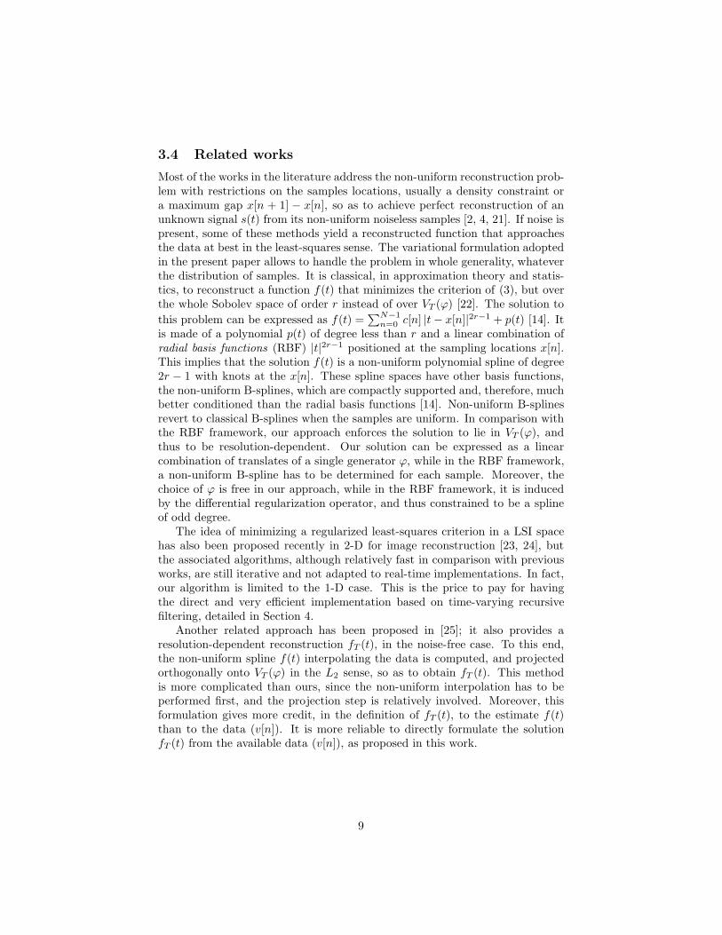
3.4 Related works

Most of the works in the literature address the non-uniform reconstruction prob-lem with restrictions on the samples locations, usually a density constraint ora maximum gap x[n + 1] − x[n], so as to achieve perfect reconstruction of anunknown signal s(t) from its non-uniform noiseless samples [2, 4, 21]. If noise ispresent, some of these methods yield a reconstructed function that approachesthe data at best in the least-squares sense. The variational formulation adoptedin the present paper allows to handle the problem in whole generality, whateverthe distribution of samples. It is classical, in approximation theory and statis-tics, to reconstruct a function f(t) that minimizes the criterion of (3), but overthe whole Sobolev space of order r instead of over VT (ϕ) [22]. The solution to

this problem can be expressed as f(t) =∑N−1

n=0 c[n] |t− x[n]|2r−1 + p(t) [14]. Itis made of a polynomial p(t) of degree less than r and a linear combination ofradial basis functions (RBF) |t|2r−1 positioned at the sampling locations x[n].This implies that the solution f(t) is a non-uniform polynomial spline of degree2r − 1 with knots at the x[n]. These spline spaces have other basis functions,the non-uniform B-splines, which are compactly supported and, therefore, muchbetter conditioned than the radial basis functions [14]. Non-uniform B-splinesrevert to classical B-splines when the samples are uniform. In comparison withthe RBF framework, our approach enforces the solution to lie in VT (ϕ), andthus to be resolution-dependent. Our solution can be expressed as a linearcombination of translates of a single generator ϕ, while in the RBF framework,a non-uniform B-spline has to be determined for each sample. Moreover, thechoice of ϕ is free in our approach, while in the RBF framework, it is inducedby the differential regularization operator, and thus constrained to be a splineof odd degree.

The idea of minimizing a regularized least-squares criterion in a LSI spacehas also been proposed recently in 2-D for image reconstruction [23, 24], butthe associated algorithms, although relatively fast in comparison with previousworks, are still iterative and not adapted to real-time implementations. In fact,our algorithm is limited to the 1-D case. This is the price to pay for havingthe direct and very efficient implementation based on time-varying recursivefiltering, detailed in Section 4.

Another related approach has been proposed in [25]; it also provides aresolution-dependent reconstruction fT (t), in the noise-free case. To this end,the non-uniform spline f(t) interpolating the data is computed, and projectedorthogonally onto VT (ϕ) in the L2 sense, so as to obtain fT (t). This methodis more complicated than ours, since the non-uniform interpolation has to beperformed first, and the projection step is relatively involved. Moreover, thisformulation gives more credit, in the definition of fT (t), to the estimate f(t)than to the data (v[n]). It is more reliable to directly formulate the solutionfT (t) from the available data (v[n]), as proposed in this work.

9

4 A fast reconstruction algorithm

4.1 Strategy

We have seen that our problem boils down to solving a linear system. It ispossible to perform this operation using standard linear algebra libraries (suchas LAPACK), that implement routines to factorize matrices in various ways andto solve linear systems. Such libraries are highly optimized, but they are generic.The practitioner interested by our approach may want to have a dedicatedalgorithm, that exploits at best the particular structure of the problem. So, wedetail in this section the best strategy for solving the linear system Ac = y.This system is symmetric, positive definite, and band-diagonal. Thus, the bestway to solve it relies on the Cholesky factorization of A and consists in thefollowing three steps:

1. The Cholesky decomposition of A is performed; that is, we compute theunique lower triangular matrix L such that A = LLT [26, 27]. L is alsoband-diagonal, with 2W diagonals containing non-zero entries: L[k, l] 6= 0only if −2W < k − l ≤ 0. The Cholesky decomposition can be performedrow by row by a fast version of Crout’s algorithm [26] that takes advantageof the band-diagonal structure of A.

2. The lower triangular system L◦c = y is solved by forward substitution: for

k from kmin to kmax,

◦cT [k] =

1

L[k, k]

(y[k]−

−1∑

i=−2W+1

L[k, k + i]◦cT [k + i]

), (18)

3. The upper triangular system LTc =◦c is finally solved by backward sub-

stitution: for k from kmax down to kmin,

cT [k] =1

L[k, k]

(◦cT [k]−

2W−1∑

i=1

L[k + i, k]cT [k + i]), (19)

4.2 Practical algorithm

The practical algorithm that computes the coefficients cT [k], k ∈ [−W +1,K +W −1], consists in two passes: the first pass implements the Cholesky decompo-sition and solves the first system (18), while the second pass solves the secondlinear system (19). We define the auxiliary variables a[i] = A[k, k + i] andu[k, i] = L[k + i, k]. Then our algorithm can be written in pseudo-code as:

10

• First pass:

for k from −W + 1 to K +W − 1 {

imin := max(−2W + 1,−W + 1− k);

imax := min(2W − 1,K +W − 1− k);

for i from 0 to imax,

a[i] :=N−1∑

n=0

ϕ(x[n]

T− k)ϕ(

x[n]

T− k − i) + λQ[k, k + i];

u[k, 0] :=(a[0]−

−1∑

i=imin

u[k + i,−i]2)1/2

;

◦cT [k] :=

1

u[k, 0]

(N−1∑

n=0

ϕ(x[n]

T− k)v[n]−

−1∑

i=imin

u[k + i,−i]◦cT [k + i]

);

for i from 1 to imax,

u[k, i] :=1

u[k, 0]

(a[i]−

−1∑

j=max(i−2W+1,−W+1−k)

u[k + j,−j]u[k + j, i− j]);

}

• Second pass:

for k from K +W − 1 down to −W + 1 {

imax := min(2W − 1,K +W − 1− k);

cT [k] :=1

u[k, 0]

(◦cT [k]−

imax∑

i=1

u[k, i]cT [k + i]);

}

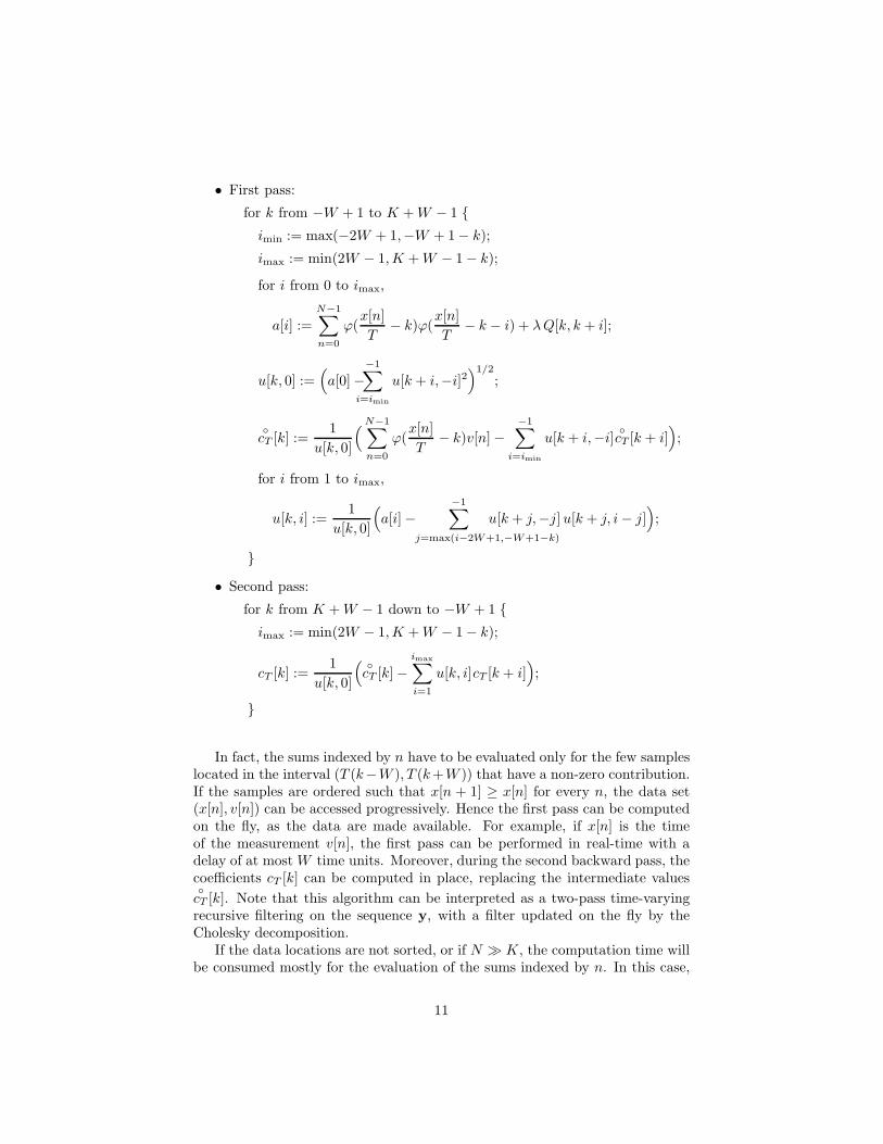
In fact, the sums indexed by n have to be evaluated only for the few sampleslocated in the interval (T (k−W ), T (k+W )) that have a non-zero contribution.If the samples are ordered such that x[n + 1] ≥ x[n] for every n, the data set(x[n], v[n]) can be accessed progressively. Hence the first pass can be computedon the fly, as the data are made available. For example, if x[n] is the timeof the measurement v[n], the first pass can be performed in real-time with adelay of at most W time units. Moreover, during the second backward pass, thecoefficients cT [k] can be computed in place, replacing the intermediate values◦cT [k]. Note that this algorithm can be interpreted as a two-pass time-varyingrecursive filtering on the sequence y, with a filter updated on the fly by theCholesky decomposition.

If the data locations are not sorted, or if N ≫ K, the computation time willbe consumed mostly for the evaluation of the sums indexed by n. In this case,

11

(a) (b)

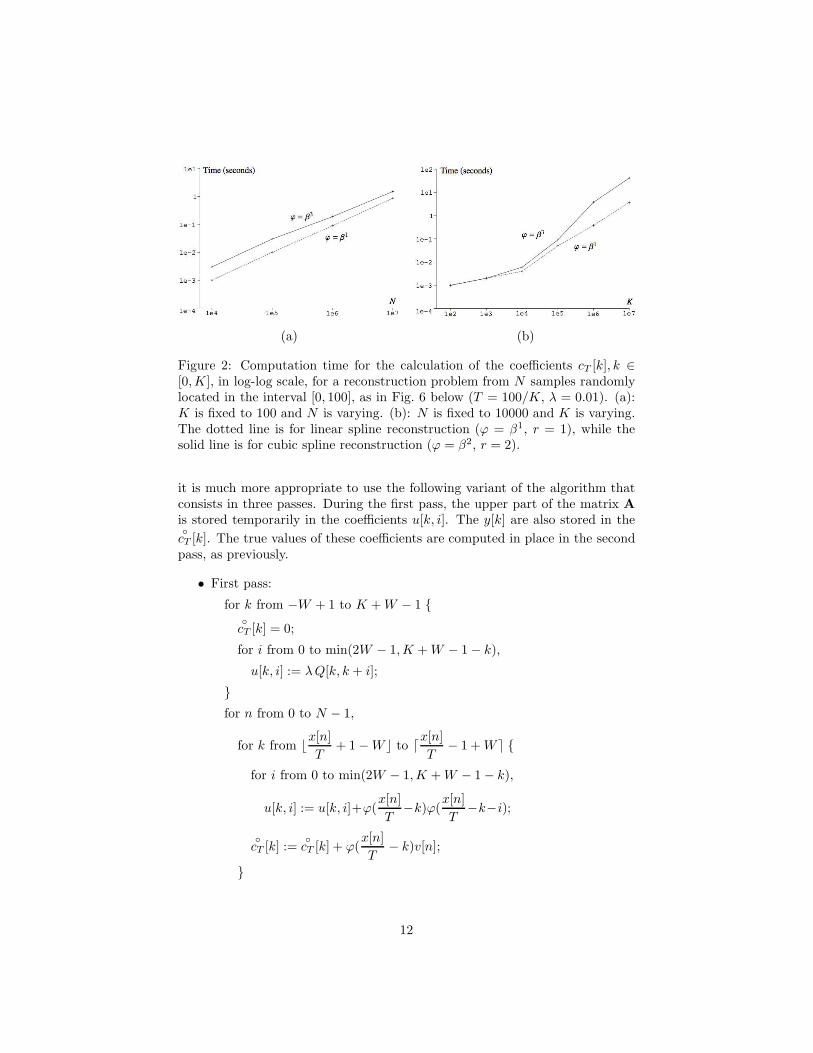
Figure 2: Computation time for the calculation of the coefficients cT [k], k ∈[0,K], in log-log scale, for a reconstruction problem from N samples randomlylocated in the interval [0, 100], as in Fig. 6 below (T = 100/K, λ = 0.01). (a):K is fixed to 100 and N is varying. (b): N is fixed to 10000 and K is varying.The dotted line is for linear spline reconstruction (ϕ = β1, r = 1), while thesolid line is for cubic spline reconstruction (ϕ = β2, r = 2).

it is much more appropriate to use the following variant of the algorithm thatconsists in three passes. During the first pass, the upper part of the matrix A

is stored temporarily in the coefficients u[k, i]. The y[k] are also stored in the◦cT [k]. The true values of these coefficients are computed in place in the secondpass, as previously.

• First pass:

for k from −W + 1 to K +W − 1 {◦cT [k] = 0;

for i from 0 to min(2W − 1,K +W − 1− k),

u[k, i] := λQ[k, k + i];

}

for n from 0 to N − 1,

for k from ⌊x[n]

T+ 1−W ⌋ to ⌈

x[n]

T− 1 +W ⌉ {

for i from 0 to min(2W − 1,K +W − 1− k),

u[k, i] := u[k, i]+ϕ(x[n]

T−k)ϕ(

x[n]

T−k−i);

◦cT [k] :=

◦cT [k] + ϕ(

x[n]

T− k)v[n];

}

12

• Second pass:

for k from −W + 1 to K +W − 1 {

imin := max(−2W + 1,−W + 1− k);

imax := min(2W − 1,K +W − 1− k);

u[k, 0] :=(u[k, 0]−

−1∑

i=imin

u[k + i,−i]2)1/2

;

◦cT [k] :=

1

u[k, 0]

(◦cT [k]−

−1∑

i=imin

u[k + i,−i]◦cT [k+i]

);

for i from 1 to imax,

u[k, i] :=1

u[k, 0]

(u[k, i]−

−1∑

j=max(i−2W+1,−W+1−k)

u[k + j,−j]u[k + j, i− j]);

}

• Third pass:

for k from K +W − 1 down to −W + 1 {

imax := min(2W − 1,K +W − 1− k);

cT [k] :=1

u[k, 0]

(◦cT [k]−

imax∑

i=1

u[k, i]cT [k + i]);

}

These algorithms are for the strategy without boundary conditions, proposedin Section 4.2. The implementation for the method with mirror boundary con-ditions is very similar. In that case, the “folding” operation on the matrices

is implemented by assigning each contribution ϕ(x[n]T − k)ϕ(x[n]T − k − i) to itsfolded place directly, for example to u[−k,−i] instead of u[k, i] if k < 0.

4.3 Computation time and storage requirements

The computation time of the proposed algorithm can be modeled as O(W 2N),O(W 2K), O(WN) for the calculation of the elements inA, L and y respectively,and O(KW ) for the forward and backward substitutions. So, the total timereduces to O(W 2(N +K)); it is linear in N and K, which is the best one couldhave hoped for. If the reconstruction is to be performed on an interval I offixed size S = KT , the total time may be rewritten O(W 2(N + S/T )), so asto let appear the linear dependence in 1/T . Experimental computation timesare reported in Fig. 2 for an implementation in C language of the algorithmproposed in Section 4.2 (second variant), running on a 1.6 GHz laptop PC. Thecomputation time is asymptotically linear in K and N , as predicted.

13

Apart of the memory required to store the coefficients cT [k], auxiliary mem-ory of size 2W (K + 2W − 1) units (or 2W (K + 1) if using mirror boundaryconditions) is needed to store the values u[k, i], which are generated during theforward pass of our algorithm and used in the backward pass.

Instead of the Cholesky decomposition, it is possible to use a LU-factorizationthat does not exploit the symmetry of the matrix. Although this decompositionrequires two times more computation, the square-root operator is not needed,and one diagonal is saved in the storage of L; that is, (2W − 1)(K + 2W − 1)instead of 2W (K + 2W − 1) memory units are used. Another variant is theLDLT factorization, that requires one more pass on the data, but also avoidsthe square-root operator.

Note that our algorithm uses a Cholesky decomposition that is “extremelystable numerically” [26]. However, even if our linear system is positive definite,its condition number clearly depends on the sampling locations. In fact, ourmethod amounts to performing the deconvolution of a time-varying filter. Inlarge gaps without samples, this filter reduces to qϕ,r, which has roots on thecomplex unit circle. An inverse filter with poles on the unit circle is said tobe marginally stable, because the impulse response corresponding to these polesdoes not decay, but does not grow either. So, if a round-off error occurs on acoefficient cT [k] during the computation, it can propagate to its neighbors insidea region without samples, but its amplitude, limited to the machine accuracy,will not grow. Therefore, this is not a problematic issue.

5 Choice of the parameters

In this section, we discuss the influence of the parameters ϕ, r, T , λ.Since the reconstruction is performed in a LSI space, this space has to be cho-

sen before hand. The “best” space depends on the characteristics of the signalto be modeled. If prior knowledge on the process that gave the samples is avail-able, it can be used to choose a particular generator ϕ [28]. For instance, if thereconstructed function is required to be continuous and continuously differen-tiable, these properties will be enforced on ϕ. In concrete problems, spline spaceshave shown to be particularly adequate for representing signals [15]. Their op-timal approximation properties have been demonstrated theoretically [29, 17]and confirmed by practical experiments [30, 31, 32]. Part of their interest liesin the fact that a B-spline has the maximal possible approximation order, giventhe size of its support. The ability to reproduce high order polynomials is ofprimary concern for approximating arbitrary signals. Besides, for a given pa-rameter r, choosing ϕ = β2r−1 ensures that our solution fT coincides with theRBF solution if the samples are uniform, at locations x[n] = Tn. This meansthat spline functions are the natural choice when minimizing a criterion basedon a derivative.

The parameter r controls the kind of smoothness that is enforced on thesolution. Three configurations are illustrated with a simple synthetic examplein Fig. 3. In (a), the choice ϕ = β1, r = 1 results in a piecewise linear recon-

14

0.4

0.6

0.8

1

1.2

1.4

0 1 2 3 4 5 6 7 8 9 100.4

0.6

0.8

1

1.2

1.4

0 1 2 3 4 5 6 7 8 9 10

(a) (b)

0.4

0.6

0.8

1

1.2

1.4

0 1 2 3 4 5 6 7 8 9 100.4

0.6

0.8

1

1.2

1.4

0 1 2 3 4 5 6 7 8 9 10

(c) (d)

Figure 3: Uniform splines with knots at the integers (T = 1, λ = 0.01) fittedon 7 point samples in the interval [0, 10], with different polynomial degrees andvalues of the regularization parameter r. (a): ϕ = β1, r = 1. (b): ϕ = β3,r = 1. (c), (d): ϕ = β3, r = 2. Mirror boundary conditions are used for (a),(b), (c), not for (d).

struction, with knots at the Tk, k ∈ Z, which means that fT (t) is linear on eachinterval [Tk, T (k+1)]. Note that with ϕ = β1, there is no other possible choicethan r = 1. Moreover, the two strategies for handling the reconstruction ona finite interval (no boundary conditions as in Section 4.2 or mirror boundaryconditions as in Section 3.3) are equivalent in this case. In (b), (c), (d), ϕ = β3

yields a smoother reconstruction, that is twice continuously differentiable. Ifr = 1, the variation

∫|∇fT |

2 is minimized, and the solution tends to behavelike a straight line in large gaps, as in (b). If r = 2, the second derivativemodelizes a curvature energy, and in large gaps, the solution fT behaves likea polynomial of degree three, as in (c); in this case, fT can go beyond the dy-namics of the initial samples, which may be a disadvantage. Note that, in largegaps, we do not have information about the signal to reconstruct. So, fitting apolynomial using the data at the boundaries of the gap is, in essence, the bestwe can do.

15

0.4

0.6

0.8

1

1.2

1.4

0 1 2 3 4 5 6 7 8 9 100.4

0.6

0.8

1

1.2

1.4

0 1 2 3 4 5 6 7 8 9 10

(a) (b)

0.4

0.6

0.8

1

1.2

1.4

0 1 2 3 4 5 6 7 8 9 100.4

0.6

0.8

1

1.2

1.4

0 1 2 3 4 5 6 7 8 9 10

(c) (d)

Figure 4: Uniform linear splines with different resolutions (ϕ = β1, r = 1,λ = 0.01) fitted on 7 point samples in the interval [0, 10]. (a): T = 0.1. (b):T = 1. (c): T = 2. (d): T = 5. The splines have their knots at the Tk,k ∈ [0, 10/T ].

The choice of the boundary conditions is illustrated in Fig. 3 (c) and (d):mirror boundary conditions yield a reconstruction whose first derivative is con-strained to be zero at the boundaries of the reconstruction interval. In this case,fT is parameterized by 11 coefficients cT [k], k ∈ [0, 10]. In (d), no boundary con-ditions are enforced, but the solution is now parameterized by 13 coefficientscT [k], k ∈ [−1, 11].

The parameter T controls the coarseness of the representation. When recon-structing a signal over an interval [0, S], we obtain a parametric solution withK + 1 = S/T + 1 degrees of freedom. If the parsimony of the representationmodeling the data is an important criterion, for instance in coding applicationsor if the computation time is limited, then T will be chosen relatively large.Conversely, when T → 0, the solution fT becomes closer and closer to the non-uniform solution in the RBF framework, since the space VT (ϕ) becomes densein the whole Sobolev space of order r. The influence of T is illustrated in Fig. 4,

16

0.4

0.6

0.8

1

1.2

1.4

0 1 2 3 4 5 6 7 8 9 100.4

0.6

0.8

1

1.2

1.4

0 1 2 3 4 5 6 7 8 9 10

(a) (b)

0.4

0.6

0.8

1

1.2

1.4

0 1 2 3 4 5 6 7 8 9 100.4

0.6

0.8

1

1.2

1.4

0 1 2 3 4 5 6 7 8 9 10

(c) (d)

Figure 5: Uniform cubic splines with knots at the integers (ϕ = β3, r = 2,T = 1, mirror boundary conditions) fitted on 7 point samples in the interval[0, 10], for different values of the smoothing parameter λ. (a): λ = 1.0. (b):λ = 0.001. (c): λ = 0.0001. (d): limit case when λ → 0.

with ϕ = β1, r = 1. The function fT is parameterized by 10/T + 1 coefficientscT [k], k ∈ [0, 10/T ]. When T → 0, fT approaches the non-uniform smoothingspline of degree 1, which has its knots at the non-uniform sampling locations.

In practical applications, the parameter T will be matched to the cut-offfrequency of the reconstruction lattice, as discussed in the next section. In fact,for each function fT ∈ VT (ϕ), there is a one-to-one correspondence between itscoefficients cT [k] and its point values wT [k] = fT (Tk) at locations Tk. That iswhy fT ∈ VT (ϕ) is said to have resolution 1/T .

The regularization factor λ is a key parameter: an excessive value will over-smooth the solution, while a small value will provide a solution that is close tothe data, but may have large disturbing variations. Let us consider the behaviorof the reconstructed function fT in the limit case when λ → 0. The solutionc = (MTM + λQ)−1MTs has a well-defined limit. This limit corresponds tosetting exactly λ = 0 in the equations only if the matrix MTM is invertible.

17

(a) (b)

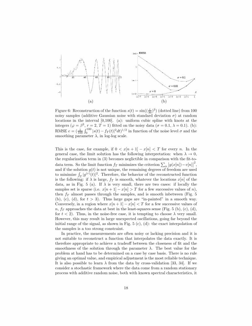
Figure 6: Reconstruction of the function s(t) = sin(( t30 )

3) (dotted line) from 100noisy samples (additive Gaussian noise with standard deviation σ) at randomlocations in the interval [0,100]. (a): uniform cubic spline with knots at theintegers (ϕ = β3, r = 2, T = 1) fitted on the noisy data (σ = 0.1, λ = 0.1). (b):

RMSE e = ( 1100

∫ 100

0 |s(t)− fT (t)|2dt)1/2 in function of the noise level σ and the

smoothing parameter λ, in log-log scale.

This is the case, for example, if 0 < x[n + 1] − x[n] < T for every n. In thegeneral case, the limit solution has the following interpretation: when λ → 0,the regularization term in (3) becomes neglictible in comparison with the fit-to-

data term. So the limit function fT minimizes the criterion∑

n

∣∣g(x[n])−v[n]∣∣2,

and if the solution g(t) is not unique, the remaining degrees of freedom are usedto minimize

∫I|g(r)(t)|2. Therefore, the behavior of the reconstructed function

is the following: if λ is large, fT is smooth, whatever the locations x[n] of thedata, as in Fig. 5 (a). If λ is very small, there are two cases: if locally thesamples set is sparse (i.e. x[n+ 1]− x[n] > T for a few successive values of n),then fT almost passes through the samples, and is smooth inbetween (Fig. 5(b), (c), (d), for t > 3). Thus large gaps are “in-painted” in a smooth way.Conversely, in a region where x[n+ 1]− x[n] < T for a few successive values ofn, fT approaches the data at best in the least-squares sense (Fig. 5 (b), (c), (d),for t < 2). Thus, in the noise-free case, it is tempting to choose λ very small.However, this may result in large unexpected oscillations, going far beyond theinitial range of the signal, as shown in Fig. 5 (c), (d): the exact interpolation ofthe samples is a too strong constraint.

In practice, the measurements are often noisy or lacking precision and it isnot suitable to reconstruct a function that interpolates the data exactly. It istherefore appropriate to achieve a tradeoff between the closeness of fit and thesmoothness of the solution through the parameter λ. The best value for theproblem at hand has to be determined on a case by case basis. There is no rulegiving an optimal value, and empirical adjustment is the most reliable technique.It is also possible to learn λ from the data by cross-validation [33, 34]. If weconsider a stochastic framework where the data come from a random stationaryprocess with additive random noise, both with known spectral characteristics, it

18

is suggested in [35] to choose λ inversely proportional to the signal-to-noise ratio.This may serve as a heuristic in the deterministic case. This is confirmed in theexample shown in Fig. 6, where λ = σ yields the minimum root-mean-squareerror, when approximating an unknown signal from its samples contaminatedby additive noise with standard deviation σ.

6 Applications

There are plenty of problems where it is useful to fit a parametric curve ondiscrete data. Numerous methods have been proposed, generally issued fromstatistical estimation theory [36]. Our approach allows to reconstruct a func-tion fT that is resolution dependent, a feature that offers many advantages inpractical applications. For example, if a non-uniform signal is to be rendered ona display device with point-spread-function Γ(t), it is straightforward to applythe proposed approach: we choose ϕ = Γ and match T to the resolution of thedevice, so that VT (ϕ) is the set of all continuously-defined signals that can berendered by the device. Therefore, by minimizing the criterion in (3), we ensurethat our solution is optimal, given the available data.

Another potential field of applications is image analysis using multiscale“pyramidal” representations. The proposed work can be used for this task, ifnot only a single function but a whole collection of functions {fT }, with differentvalues of T , is computed. For instance, the performances of procedures such asedge detection or image registration can be improved by processing from coarserto finer levels [37]. To this purpose, our approach is more general than classicaldyadic representations, that only apply to uniform signals and discrete dyadicresolutions (T = 2n, n ∈ N).

Our approach is also particularly adapted to resampling problems involvingrate conversions, such as image resizing. Let us present some generic problemsthat could benefit from our approach.

6.1 Non-uniform to uniform resampling

Given the non-uniform samples v[n] at locations x[n], suppose we want to obtainresampled values wT [k] located on the uniform reconstruction lattice (Tk)k∈Z.We can simply compute the function fT (t) and resample it on the uniformlattice: this yields wT [k] = fT (Tk) for every k. In fact, once the cT [k] havebeen computed, the signal wT is directly obtained by digital filtering [15]: wT =cT ∗ b−1, where b[k] = ϕ(k) for every k ∈ Z.

With this method, the representation capabilities of the target lattice, wherethe resampled signal lives, are exploited optimally: fT (t) retains at best theinformation contained in the non-uniform samples and representable on thislattice. Conversely, the information that is not representable is canceled out,and no irrelevant structure is introduced. As a consequence, the aliasing issueis automatically handled because, qualitatively, the frequencies higher than theNyquist rate of the target lattice are not representable in VT (ϕ). That is why

19

(a) (b) (c)

(d) (e) (f)

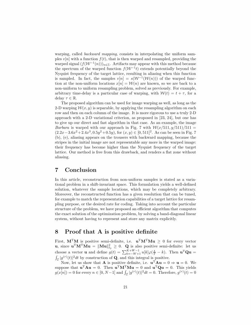
Figure 7: Image Barbara (a) warped using: backward mapping (b), and pro-posed approach with λ = 10−4 (c) (see text). (d), (e), (f): zoom-ins on (a), (b),(c) respectively.

T is chosen so that fT has a resolution matched to the cut-off frequency of thereconstruction lattice. Note that we assume that ϕ is lowpass, and that λ iscorrectly chosen so as not to distort the frequency content of the data.

This approach is also useful for resampling a uniform (x[n] = n) signal v. Ifv is to be resampled at coarser resolution or magnified with a non-integer fac-tor, interpolation followed by resampling can introduce severe distortions [38].Instead, we look for a function having the resolution of the target resampled sig-nal, and not of the source signal. This formulation has been proposed previouslyin [39], in the more restrictive case where T is an integer.

Interestingly, our approach amounts to formulate resampling as an inverseproblem: we seek the uniform signal wT that, when interpolated by the functionfT (t) and resampled back on the source lattice (x[n]), is the closest to the initialsignal (v[n]). This is the opposite of the forward approach that fits a function onthe source signal, typically by interpolation, and then resample it, independentlyof the target lattice.

6.2 Warping

Another application is signal or image warping. Suppose we have the uni-form samples v[n] = s(n) of an unknown function s(t) at our disposal, and wewant to compute the uniform samples (s(W−1(n)))n∈Z of the warped functions(W−1(t)) for some reversible transform W(t). The classical method used for

20

warping, called backward mapping, consists in interpolating the uniform sam-ples v[n] with a function f(t), that is then warped and resampled, providing thewarped signal (f(W−1(n)))n∈Z. Artifacts may appear with this method becausethe spectrum of the warped function f(W−1t) extends potentially beyond theNyquist frequency of the target lattice, resulting in aliasing when this functionis sampled. In fact, the samples v[n] = s(W−1(W(n))) of the warped func-tion at the non-uniform locations x[n] = W(n) are known, so we are back to anon-uniform to uniform resampling problem, solved as previously. For example,arbitrary time-delay is a particular case of warping, with W(t) = t + τ , for adelay τ ∈ R.

The proposed algorithm can be used for image warping as well, as long as the2-D warpingW(x, y) is separable, by applying the resampling algorithm on eachrow and then on each column of the image. It is more rigorous to use a truly 2-Dapproach with a 2-D variational criterion, as proposed in [23, 24], but one hasto give up our direct and fast algorithm in that case. As an example, the imageBarbara is warped with our approach in Fig. 7 with W(x/511, y/511)/511 =(2.2x−3.6x2+2.4x3, 0.5y2+0.5y), for (x, y) ∈ [0, 511]2. As can be seen in Fig. 7(b), (e), aliasing appears on the trousers with backward mapping, because thestripes in the initial image are not representable any more in the warped image:their frequency has become higher than the Nyquist frequency of the targetlattice. Our method is free from this drawback, and renders a flat zone withoutaliasing.

7 Conclusion

In this article, reconstruction from non-uniform samples is stated as a varia-tional problem in a shift-invariant space. This formulation yields a well-definedsolution, whatever the sample locations, which may be completely arbitrary.Moreover, the reconstructed function has a given resolution that can be tuned,for example to match the representation capabilities of a target lattice for resam-pling purpose, or the desired rate for coding. Taking into account the particularstructure of the problem, we have proposed an efficient algorithm that computesthe exact solution of the optimization problem, by solving a band-diagonal linearsystem, without having to represent and store any matrix explicitly.

8 Proof that A is positive definite

First, MTM is positive semi-definite, i.e. uTMTMu ≥ 0 for every vectoru, since uTMTMu = ‖Mu‖2ℓ2 ≥ 0. Q is also positive semi-definite: let us

choose a vector u and define g(t) =∑K+W−1

k=−W+1 u[k]ϕ(tT − k). Then uTQu =∫

I|g(r)(t)|2dt by construction of Q, and this integral is positive.Now, let us show that A is positive definite, i.e. uTAu = 0 ⇒ u = 0. We

suppose that uTAu = 0. Then uTMTMu = 0 and uTQu = 0. This yieldsg(x[n]) = 0 for every n ∈ [0, N−1] and

∫I|g(r)(t)|2dt = 0. Therefore, g(r)(t) = 0

21

within I, and g(t) is a polynomial of degree less than r in this interval. Thispolynomial has N roots at the x[n] (with at least r distinct roots by hypothesison the samples locations). Then g = 0 and u[k] = 0 for every k. �

References

[1] C. E. Shannon, “Communication in the presence of noise,” Proc. of the

Inst. of Radio Eng., vol. 37, no. 1, pp. 10–21, 1949.

[2] K. Grochenig and H. Razafinjatovo, “On Landau’s necessary density con-ditions for sampling and interpolation of band-limited functions,” J. Lond.

Math. Soc., vol. 54, no. 3, pp. 557–567, 1996.

[3] W. Chen and S. Itoh, “A sampling theorem for shift-invariant subspaces,”IEEE Trans. Signal Processing, vol. 46, no. 10, pp. 2822–2824, Oct. 1998.

[4] A. Aldroubi and K. Grochenig, “Beurling-Landau-type theorems for non-uniform sampling in shift invariant spline spaces,” J. Fourier Anal. Appl.,vol. 6, no. 1, pp. 93–103, 2000.

[5] H. G. Feichtinger, K. Grochenig, and T. Strohmer, “Efficient numericalmethods in non-uniform sampling theory,” Numer. Math., no. 4, pp. 423–440, 1995.

[6] T. Strohmer, “Numerical analysis of the non-uniform sampling problem,”J. Comp. Appl. Math., vol. 112, no. 1-2, pp. 297–316, 2000.

[7] Y. Liu, “Irregular sampling for spline wavelet subspaces,” IEEE Trans.

Inform. Theory, vol. 42, no. 2, pp. 623–627, 1996.

[8] A. Aldroubi and K. Grochenig, “Nonuniform sampling and reconstructionin shift-invariant spaces,” SIAM Rev., vol. 43, no. 4, pp. 585–620, 2001.

[9] W. Chen, B. Han, and R.-Q. Jia, “Maximal gap of a sampling set for theexact iterative reconstruction algorithm in shift-invariant spaces,” IEEE

Signal Processing Lett., vol. 11, no. 8, pp. 655–658, Aug. 2004.

[10] C. D. Boor, R. DeVore, and A. Ron, “The structure of finitely generatedshift-invariant spaces in L2(R

d),” J. Funct. Anal. 119, pp. 37–78, 1994.

[11] R.-Q. Jia, “Shift-invariant spaces and linear operator equations,” Israel J.

Math., vol. 41, pp. 259–288, 1998.

[12] I. Daubechies, Ten lectures on wavelets. Philadelphia, PA, USA: Societyfor Industrial and Applied Mathematics, 1992.

[13] M. Unser, “Sampling—50 Years after Shannon,” Proc. IEEE, vol. 88, no. 4,pp. 569–587, Apr. 2000.

22

[14] C. de Boor, A Practical Guide to Splines. New York: Springer-Verlag,1978.

[15] M. Unser, “Splines: A perfect fit for signal and image processing,” IEEE

Signal Processing Mag., vol. 16, no. 6, pp. 22–38, Nov. 1999.

[16] M. Jacob, T. Blu, and M. Unser, “Efficient energies and algorithms forparametric snakes,” IEEE Trans. Image Processing, vol. 13, no. 9, pp.1231–1244, Sep. 2004.

[17] T. Blu, P. Thevenaz, and M. Unser, “Moms: Maximal-order interpolationof minimal support,” IEEE Trans. Image Processing, vol. 10, no. 7, pp.1069–1080, Jul. 2001.

[18] R. Madani, A. Ayremlou, A. Amini, and F. Marvasti, “Optimized compact-support interpolation kernels,” IEEE Trans. Signal Processing, vol. 60,no. 2, pp. 626–633, Feb. 2012.

[19] L. Rudin, S. Osher, and E. Fatemi, “Nonlinear total variation based noiseremoval algorithms,” Physica D, vol. 60, no. 1–4, pp. 259–268, 1992.

[20] C. M. Brislawn, “Classification of nonexpansive symmetric extension trans-forms for multirate filter banks,” Applied and Comp. Harmonic Anal.,vol. 3, pp. 337–357, 1996.

[21] K. Grochenig and H. Schwab, “Fast local reconstruction methods fornonuniform sampling in shift invariant spaces,” SIAM J. Matrix Anal. and

Appl., vol. 24, no. 4, pp. 899–913, 2003.

[22] R. L. Eubank, Nonparametric regression and spline smoothing. New York,NY, USA: Marcel Dekker, 1999.

[23] M. Arigovindan, M. Suhling, P. Hunziker, and M. Unser, “Variational im-age reconstruction from arbitrarily spaced samples: A fast multiresolutionspline solution,” IEEE Trans. Image Processing, vol. 14, no. 4, pp. 450–460,Apr. 2005.

[24] C. Vazquez, E. Dubois, and J. Konrad, “Reconstruction of nonuniformlysampled images in spline spaces,” IEEE Trans. Image Processing, vol. 14,no. 6, pp. 713–725, Jun. 2005.

[25] A. Munoz Barrutia, T. Blu, and M. Unser, “Non-uniform to uniform gridconversion using least-squares splines,” in Proc. of EUSIPCO, vol. 4, Tam-pere, Finland, Sep. 2000, pp. 1997–2000.

[26] W. H. Press, S. A. Teukolsky, W. T. Vetterling, and B. P. Flannery, Nu-merical Recipes in C: The Art of Scientific Computing. New York, NY,USA: Cambridge University Press, 1992.

[27] G. H. Golub and C. F. V. Loan, Matrix computations, 2nd ed. Baltimore:Johns Hopkins Univ. Press, 1989.

23

[28] S. Ramani, D. Van De Ville, and M. Unser, “Sampling in practice: Is thebest reconstruction space bandlimited?” in Proc. of IEEE ICIP, vol. 2,Sep. 2005, pp. 153–156.

[29] T. Blu and M. Unser, “Quantitative Fourier analysis of approximationtechniques: Part I–interpolators and projectors—and part II–wavelets,”IEEE Trans. Signal Processing, vol. 47, no. 10, pp. 2783–2806, Oct. 1999.

[30] T. M. Lehmann, C. Gonner, and K. Spitzer, “Survey: Interpolation meth-ods in medical image processing,” IEEE Trans. Med. Imag., vol. 18, no. 11,pp. 1049–1075, Nov. 1999.

[31] P. Thevenaz, T. Blu, and M. Unser, “Interpolation revisited,” IEEE Trans.

Med. Imag., vol. 19, no. 7, pp. 739–758, Jul. 2000.

[32] E. Meijering, W. Niessen, and M. Viergever, “Quantitative evaluation ofconvolution-based methods for medical image interpolation,” Medical Im-

age analysis, vol. 5, no. 2, pp. 111–126, Jun. 2001.

[33] P. Craven and G. Wahba, “Smoothing noisy data with spline functions:Estimating the correct degree of smoothing by the method of generalizedcross-validation,” Numerical Mathematics, vol. 31, pp. 377–403, 1979.

[34] M. F. Hutchinson and F. R. De Hoog, “Smoothing noisy data with splinefunctions,” Numer. Math., vol. 4, no. 7, pp. 99–106, 1985.

[35] Y. C. Eldar and M. Unser, “Non-ideal sampling and interpolation fromnoisy observations in shift-invariant spaces,” IEEE Trans. Signal Process-

ing, vol. 54, no. 7, pp. 2636–2651, Jul. 2006.

[36] G. Wahba, Spline models for observational data. Philadelphia, PA: Societyfor industrial and applied mathematics (SIAM), 1990.

[37] P. Thevenaz, U. E. Ruttimann, and M. Unser, “A pyramid approach tosubpixel registration based on intensity,” IEEE Trans. Image Processing,vol. 7, no. 1, pp. 27–41, Jan. 1998.

[38] M. Unser, A. Aldroubi, and M. Eden, “Enlargement or reduction of digitalimages with minimum loss of information,” IEEE Trans. Image Processing,vol. 4, no. 3, pp. 247–258, Mar. 1995.

[39] A. Aldroubi, M. Eden, andM. Unser, “Discrete spline filters for multiresolu-tion and wavelets of l2,” SIAM J. Math. Anal., vol. 25, no. 5, pp. 1412–1432,Sep. 1994.

24