FEDERAL RESERVE BANK OF ST. LOUIS Research Division

P.O. Box 442 St. Louis, MO 63166

______________________________________________________________________________________

The views expressed are those of the individual authors and do not necessarily reflect official positions of the Federal Reserve Bank of St. Louis, the Federal Reserve System, or the Board of Governors.

Federal Reserve Bank of St. Louis Working Papers are preliminary materials circulated to stimulate discussion and critical comment. References in publications to Federal Reserve Bank of St. Louis Working Papers (other than an acknowledgment that the writer has had access to unpublished material) should be cleared with the author or authors.

RESEARCH DIVISIONWorking Paper Series

Nominal GDP Targeting With Heterogeneous Labor Supply

James Bullard and

Aarti Singh

Working Paper 2017-016Ahttps://doi.org/10.20955/wp.2017.016

February 2017

Nominal GDP Targeting withHeterogeneous Labor Supply

James Bullard∗ Aarti Singh†

This version: 17 February 2017‡

Abstract

We study nominal GDP targeting as optimal monetary policy in amodel with a credit market friction following Azariadis, Bullard, Singhand Suda (2016), henceforth ABSS. As in ABSS, the macroeconomy westudy has considerable income inequality which gives rise to a large pri-vate sector credit market. Households participating in this market usenon-state contingent nominal contracts (NSCNC). We extend the ABSSframework to allow for endogenous and heterogeneous household laborsupply among credit market participant households. We show that nom-inal GDP targeting continues to characterize optimal monetary policy inthis setting. Optimal monetary policy repairs the distortion caused by thecredit market friction and so leaves heterogeneous households supplyingtheir desired amount of labor, a type of “divine coincidence” result. Wealso analyze the case when there is an aging population. We interpretthese findings in light of the recent debate in monetary policy concerninglabor force participation.

Keywords : Non-state contingent nominal contracting, optimal mone-tary policy, nominal GDP targeting, life cycle economies, heterogeneoushouseholds, credit market participation, labor supply. JEL codes : E4, E5.

∗Federal Reserve Bank of St. Louis; james.b.bullard@stls.frb.org. Any views expressed arethose of the authors and do not necessarily reflect the views of others on the Federal OpenMarket Committee.†Corresponding author. University of Sydney; aarti.singh@sydney.edu.au.‡We thank Thomas Sargent, David Andolfatto, Chung-Shu Wu, Been-Lon Chen and sem-

inar participants at Bank of Korea’s 2016 Policy Conference, Academia Sinica, Society forComputational Economics and Finance 2016 and London School of Economics for their con-structive input.

1 Nominal GDP targeting

1.1 Overview

Recent papers by Sheedy (2014), Koenig (2013), and Azariadis, Bullard, Singh

and Suda (2016), hereafter ABSS, provide analyses of optimal monetary pol-

icy in economies where the key friction is in the credit market in the form of

non-state contingent nominal contracting (NSCNC). They all show that optimal

policy can be characterized as a version of nominal GDP targeting in that en-

vironment. The monetary policy provides a form of insurance to private sector

credit-using households.

The ABSS model is based on credit-using households with inelastic labor

supply. An open question is whether the optimal monetary policy they isolate

could continue to be characterized as nominal GDP targeting if credit-using

households were allowed to adjust labor supply in response to shocks. In prin-

ciple, these (heterogeneous) households may be able to partially self-insure in

this circumstance, thus altering the nature of the nominal GDP targeting policy

or even rendering it unnecessary. Our goal is to study this issue in this paper.

We construct an extension of the life cycle framework of ABSS (2016) to a

case of endogenous (and heterogeneous) labor supply.1 Credit-using households

have homothetic preferences defined over consumption and leisure choices. We

also include population growth in the model, in order to be able to comment on

whether the changing nature of the workforce would have any implications for

our findings. We compare our findings to some labor market data for the U.S.

economy, but we do not consider this version of the model to be sophisticated

enough to compare to data in a more comprehensive way.2

Our main finding is that nominal GDP targeting continues to characterize

the optimal monetary policy in the situation with endogenous and heteroge-

neous labor supply and constant population growth. The policy completely

repairs the distortion caused by the NSCNC friction and allows all credit-using

1Sheedy (2014) and Koenig (2013) also consider labor supply in their models. In our modelwe have more than two types of agents and that it is not clear how endogenous labor supplywould impinge on the NGDP targeting result in that case.

2We hope to take up the challenge of matching data more comprehensively in future versionsof the model.

1

households to consume equal amounts at each date. This is the hallmark of

the NGDP targeting policy in this model– under this policy credit markets are

characterized by “equity share”contracting, which is optimal when preferences

are homothetic.

Our main result is a version of the “divine coincidence”result familiar from

the New Keynesian monetary policy literature.3 In our model, there is a single

friction, which is non-state contingent nominal contracting in the credit sector.

Monetary policy can alter the price level to eliminate the distortion arising from

this friction and restore the first-best allocation of resources. Our main result

shows that, in this situation, households are able to choose their optimal level

of labor supply as well, and in fact these heterogeneous labor supply choices

are independent of the aggregate shock in the model. The divine coincidence is

that, by completely mitigating the credit market friction, the monetary policy

also allows for optimal labor supply choices.

Our main result suggests that optimal monetary policy can be conducted

in this environment without reference to labor market outcomes. Labor supply

growth would in this situation be closely related to labor force growth, as it is

in the U.S. data. An economy in this class could have an aging workforce if the

labor force growth rate is slowing over time. In this situation the comparative

statics of the model predict that as the workforce ages, younger cohorts will

work less and older cohorts will work more. This is indeed what has happened

in the U.S. data over the last 20 years, as we show near the end of the paper.

We take this as one indication that the forces influencing labor supply in this

model may also be influencing labor supply in the U.S. economy.

1.2 Additional motivation

Aside from the issue of whether the NGDP targeting policy remains optimal

in the face of endogenous labor supply in this setting, we additionally motivate

the paper with a contemporary issue in monetary policy. Since the 2007-2009

financial crisis, the labor force participation rate in the U.S. has been low and

3See Blanchard and Gali (2010) and Woodford (2003).

2

falling.4 A key question for monetary policymakers has been whether the falling

labor force participation rate is driven by business cycle factors, in which case

monetary policymakers may want to attempt to increase the participation rate

through monetary policy choices. But an alternative, and we think more tradi-

tional, view is that the labor force participation rate is driven by demographic

factors, in which case policymakers will be unable to meaningfully change the

participation rate via monetary policy. The results in this paper provide some

support for the traditional view.

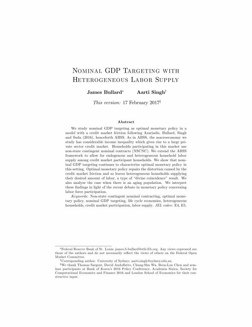
Figure 1 is the first figure from Erceg and Levin (2014). They suggest, based

on this evidence from 2004-2013, that labor force participation fell much more

than expected by some government agencies in the aftermath of the financial

crisis and recession of 2007-2009 in the U.S. They construct a New Keynesian

model of monetary policy in which the labor force participation rate would not

be an important cyclical variable in normal times, but which may remain sig-

nificantly depressed following a particularly large macroeconomic shock. They

find that monetary policy may be able to help mitigate an ineffi ciently low level

of labor force participation.

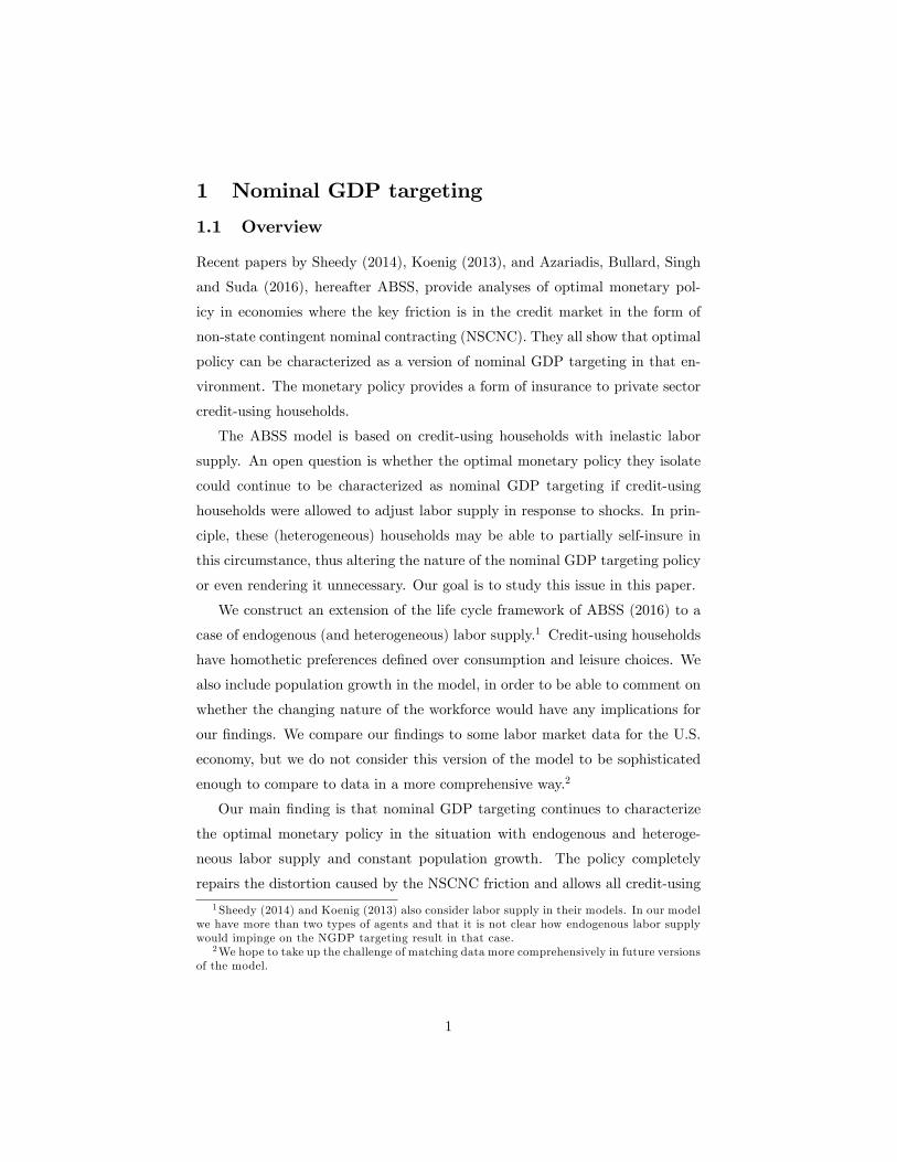
Figure 2 offers a different take on the same data. This Figure again shows

the U.S. labor force participation rate, the solid line, this time from 1991-2015.

The figure also shows a forecast labor force participation rate due to Aaronson,

Fallick, Figura, Pingle, and Wascher (2006), represented by the dotted line

in the figure. The Aaronson, et al., (2006) model is based importantly on

demographic effects. Their 2006 model successfully predicted the decline in

labor force participation as of the 2013 to 2015 time frame, about 7 to 9 years

in the future.5 We think of the Aaronson, et al., (2006) findings as consistent

with what we see as a “traditional view”in macroeconomics, whereby labor force

participation is an essentially acyclical variable, movements in which would not

be indicative of business cycle developments but would rather reflect longer-run

4The literature documenting the fall in the labor force participation rate is growing. See forexample, Aaronson, Cajner, Fallick, Galbis-Reig, Smith and Wascher (2016), Van Zandweghe(2012), Daly, Elias, Hobijn and Jordà (2012), Hotchkiss and Rios-Avila (2013) among others.

5Hall and Petrosky-Nadeau (2016), Daly et. al. (2012) among others also attribute declin-ing labor force participation rates to ongoing secular change in trend. In a recent paper,Krueger (2016) plots a forecast of the labor force participation rate from 2007 to 2016. Thatplot exhibits a declining pattern similar to the one shown in Figure 2.

3

Figure 1: The first figure, left panel, from Erceg and Levin (2014). After thefinancial crisis and recession of 2007-2009, labor force participation in the U.S.fell more than its forecast by leading government agencies.

changes in desired labor supply by the workforce in the economy. These longer-

run movements would then be viewed as largely independent of monetary policy

choices.

In the current paper, we will present a model which is consistent with what

we call the traditional view of labor force participation. In the model, monetary

policy will have an important role to play in ensuring good credit market perfor-

mance. If this monetary policy is carried out in the optimal manner (which will

turn out to be our version of nominal GDP targeting), then labor supply choices,

while heterogeneous, will indeed be independent of monetary policy and of the

shocks buffeting the economy.6 Furthermore, we will have population growth in

the model, and we will use this feature to show how changing demographics may

cause changing labor supply phenomena in the economy while not interfering

with the central bank’s ability to deliver a first-best policy.7

6Here the phrase “independent of monetary policy”is meant to convey the idea that, whilethe policymaker is changing the price level in response to aggregate productivity shocks, thehouseholds do not wish to change their labor supply in response to the price level movements.

7For an extensive discussion of demographic trends and their associated effects on laborforce participation, see Krueger (2016). For a review of some of the recent literature andconnections to current monetary policy issues, see Bullard (2014).

4

Figure 2: Labor force participation in the U.S., 1991-2015. The dotted linerepresents the forecast made by Aaronson et al (2006) using a model basedlargely on demographic factors. The forecast is essentially correct even 7 to 9years in the future.

2 Environment

2.1 The private sector

2.1.1 Background on symmetry

ABSS (2016) work with a stylized general equilibrium life cycle economy with

an aggregate shock to productivity growth. This means that the economy has

heterogeneous households along with an aggregate shock, and therefore that

the equilibrium includes tracking the asset-holding distribution in the economy.

However, to keep the heterogeneity manageable and the equilibrium calculable

based on closed-form solutions, ABSS (2016) made certain “stylized symmetry

assumptions.” In the life cycle model, much depends on the productive capac-

ity of older cohorts, the suppliers of credit, versus the productive capacity of

younger cohorts, the demanders of credit. The goal is to keep this aspect of the

model in balance via simplifying assumptions. Accordingly, the productivity

endowments of credit-using households are assumed to be perfectly symmetric,

peaking in the middle period of life. In addition, there is no discounting of the

future in the preferences (that is, the discount factor β = 1), which would other-

5

wise tend to favor consumption today over consumption tomorrow.8 Combined

with time-separable log preferences, these assumptions help make the key quan-

tities in the model– including the net asset positions of all households– linear

in the real wage. This means that the asset-holding distribution can be tracked

easily. The equilibrium real interest rate on loans is then exactly equal to the

real output growth rate each period, even in the stochastic case. Altogether,

this creates a particularly tractable framework in which the intuition behind the

nominal GDP targeting policy is brought into clearer relief.

We will maintain these same stylized symmetry assumptions in this paper

as well. However, by adding population growth in this paper, the symmetry

underlying the ABSS (2016) model will be slightly disturbed. In particular,

with constant population growth there will be “too much”productive capacity

in the younger cohorts (that is, too much population mass in those cohorts given

the productivity endowments), and not enough in the older cohorts. To restore

symmetry, we will therefore allow publicly-issued debt as an asset in this paper

in order to again create an equilibrium where the real interest rate on loans is

equal to the real output growth rate each period, as in ABSS (2016). The fiscal

authority will issue just enough debt each period to pay principal and interest

on previously-issued debt, and this assumption will have no other role to play

in this version of the model.

2.1.2 Cohorts and segmented markets

We now turn to describing the model in more detail. Following ABSS (2016),

we use a life cycle model with segmented markets. Cohorts are collections

of identical, atomistic households entering and later exiting the economy at

the same date. Cohorts are divided into two types, a large group of “credit

market participants”and a small group of “credit market non-participants.”We

also refer to these two groups as “credit users”and “cash users,” respectively.

Households live in discrete time for T +1 periods. Our results will hold for any

integer T ≥ 2, but for most presentation purposes we will use the value T +1 =241 so that we can interpret results as corresponding to a quarterly model in

8We could add discounting back in, at the cost of minor complications. It is unnecessaryin this type of model and so we omit it for simplicity.

6

which households begin and end economic life with zero assets, starting, let’s say,

around age 20, and continuing until death. Choosing T+1 to be an odd number

allows for a convenient and specific peak period for participant productivity

endowment profiles. The economy itself continues into the infinite past and into

the infinite future, with discrete time denoted by t where −∞ < t < ∞. Theassets in the economy are privately-issued nominal debt, publicly-issued nominal

debt, and currency. Credit market participant households can hold any of these

assets, but in the equilibria we study, they will only hold the two types of debt,

which will each pay an identical real rate of return always higher than the real

rate of return on holding currency.9 Cash-using households are excluded from

credit markets altogether and only hold currency. All loan contracts are for one

period, are not state-contingent, and are expressed in nominal terms– we call

this the non-state contingent nominal contracting (NSCNC) friction.

The extension in this paper relative to ABSS (2016) is to add endogenous

labor supply and population growth.

2.1.3 Population growth

We think of the participant portion of the cohort entering the economy at date

t as having measure nt, for any date t.10 These cohort sizes are related by a

constant gross growth rate ψ ≥ 1, as

nt = ψnt−1 (1)

with n0 > 0. The participant population at date t can then be measured as

N (t) = nt + nt−1 + · · ·+ nt−T (2)

= nt

[1 + ψ−1 + ψ−2 + · · ·+ ψ−T

]. (3)

Similarly the participant population at t− 1 would be

N (t− 1) = nt−1

[1 + ψ−1 + ψ−2 + · · ·+ ψ−T

]. (4)

9That is, nominal interest rates will always be positive.10We generally follow the notational convention that subscript t indicates the cohort (the

“birth date”) and that t in parentheses denotes real time. The exception to this is theproductivity endowment notation as described below.

7

The gross participant population growth rate is therefore equal toN (t) //N (t− 1) =ψ.

We think of the relatively small non-participant portion of the cohort enter-

ing the economy at date t symmetrically. They have measure mt at date t, a

constant gross growth rate of ψ, and a gross non-participant population growth

rate of ψ. Since mt+nt = 1, the overall population growth rate is also ψ. Since

all households work at least some of the time in this model, the population

growth rate is also the labor force growth rate.

2.1.4 Participant productivity endowments

Credit market participant households enter the economy endowed with a known

sequence of productivity units given by e = {es}Ts=0 . This notation means thateach household entering the economy has productivity endowment e0 in the first

period of activity, e1 in the second, and so on up to eT . In order to keep the model

simple and stylized, we assume that this productivity endowment sequence is

hump-shaped and symmetric (that is, e0 = eT , e1 = eT−1, e2 = eT−2...) and

that it peaks exactly at the middle period of life. We use the following profile:

es = f (s) = µ0 + µ1s+ µ2s2 + µ3s

3 + µ4s4 (5)

such that f (0) = 0.5, f (60) = 0.8, f (120) = 1, f (180) = 0.8, and f (240) = 0.5.

This is a stylized endowment profile which emphasizes that near the beginning

and end of the life cycle productivity is low, while in the middle of the life

cycle it is high. This endowment profile is displayed in Figure 1. Participant

households can sell the productivity units they are endowed with each period

on a labor market at a economy-wide competitive wage per effi ciency unit.

This particular profile is useful for illustrating the points we wish to empha-

size in this paper. The profile suggests that productivity is relatively low at the

beginning and end of economic life, but not so low that households might be

tempted to supply zero labor in those circumstances. This means that we can

restrict attention to interior solutions for the equilibria we study.

8

50 100 150 200Coh ort

0 .5

0 .6

0 .7

0 .8

0 .9

1 .0

Productiv ityEndowment

Figure 3: A schematic productivity endowment profile for credit market partic-ipant households. The profile is symmetric and peaks in the middle period ofthe life cycle. The income distribution at each date is this profile multiplied bythe real wage. There is considerable income inequality.

2.1.5 Participant household preferences

We denote all variables in real terms except for nominal asset holding a, which

is in nominal terms to allow analysis of the NSCNC friction. Accordingly, we let

ct (t+ s) > 0 denote the date t+s real consumption of the household entering the

economy at date t (that is, the date of entry into the economy– the cohort– is

indicated by the subscript in this notation), and where `t (t+ s) ∈ (0, 1) denotesthe date t+s leisure of the household entering the economy at date t, where the

household has one unit of time each period of life. The discount factor β = 1

and η ∈ (0, 1] controls the intratemporal consumption-leisure trade-off. Creditmarket participant households entering the economy at date t with no asset

holdings have preferences given by

Ut =

T∑s=0

η ln ct (t+ s) + (1− η) ln `t (t+ s) . (6)

There are also credit market participant households that entered the economy

at date t− 1. These households have preferences given by

Ut−1 =

T−1∑s=0

η ln ct−1 (t+ s) + (1− η) ln `t−1 (t+ s) . (7)

9

These households will also have a net asset position which we denote by at−1 (t− 1) ,which indicates the net asset holdings carried into the current period from date

t − 1 by the cohort that entered the economy at date t − 1. Other house-

hold preferences for participant households that entered the economy at dates

t − 2, ..., t − T are defined analogously, with net asset positions at−2 (t− 1) ,..., at−T (t− 1) .

2.1.6 Non-participant productivity endowments and preferences

The non-participant households are precluded from using the credit market.

They provide a demand for currency in this economy. These households live for

T + 1 periods like their credit market participant cousins, and we will discuss

them in terms of their stage of life 0, 1, 2, ..., T. Their productivity endowment

pattern is very different from credit market participant households. In the

first period of life they are inactive. Thereafter, in odd-dated stages of life,

these households have a productivity endowment γ ∈ (0, 1) . We think of thisas being a low value, and there is no life cycle aspect to it. The cash-using

households entering the economy at date t then supply labor inelastically and

earn income γw (t+ s) for s = 1, 3, 5, ..., T − 1. In even-dated stages of life,the non-participant households consume. Their period utility is ln ct (t+ s) ,

s = 2, 4, 6, ..., T. These agents work intermittently, carrying the value of their

labor income via currency holdings into the period when they wish to consume.

The non-participant household problem generates a conventional currency

demand. For brevity, we omit further description of this problem here and refer

readers to ABSS (2016). The cash-using households are motivated by an appeal

to the unbanked sector of the U.S. economy, which has been estimated to be on

the order of 10 to 15 percent of U.S. households.

2.1.7 Technology

The technology is simple extension of the endowment economy idea that “one

unit of labor produces one unit of the good,”but with appropriate adjustments

for productivity endowments e and labor supply 1− `t (t) . We denote the levelof TFP as Q (t) . The gross growth rate of Q follows a stochastic process such

10

that

Q (t) = λ (t− 1, t)Q (t− 1) , (8)

where λ (t− 1, t) is the growth rate of productivity between date t− 1 and datet. The stochastic process driving the growth rate of productivity is AR (1) with

mean λ,

λ (t, t+ 1) = (1− ρ)λ+ ρλ (t− 1, t) + σε (t+ 1) (9)

where the unadorned λ > 1 is the mean growth rate, serial correlation ρ ∈ (0, 1) ,σ > 0 is a scale factor, and ε (t) ∼ N (0, 1) .11 Aggregate output is given by

Y (t) = Q (t)L (t) . (10)

where L (t) is the total supply of labor in this economy.

If we denote 1− `t (t) ∈ (0, 1) as the fraction of participant household timespent working per period, the labor input at date t is given by

Lp (t) = e0nt (1− `t (t)) + e1nt−1 (1− `t−1 (t)) + · · ·+ eTnt−T (1− `t−T (t))(11)

and the supply of labor by non-participants is simply

Lnp (t) = [mt−1 +mt−3 + · · ·+mt−T+1] γ (12)

The marginal product of labor is

w (t) = Q (t) (13)

and we conclude that

w (t) = λ (t− 1, t)w (t− 1) (14)

as in ABSS (2016). The aggregate output growth rate is then

Y (t)

Y (t− 1) =Q (t)L (t)

Q (t− 1)L (t− 1) = λ (t− 1, t) L (t)

L (t− 1) . (15)

11This stochastic process will imply that the zero lower bound on the nominal interest ratecan be encountered in this economy, because the shock can always be suffi ciently negative.However, a version of the nominal GDP targeting monetary policy can address this situationwhen η = 1 (inelastic labor supply) and ψ = 1 (no population growth) as discussed in ABSS(2016). We will not address ZLB issues in this paper.

11

What is L (t) /L (t− 1)? We can write

L (t)

L (t− 1) =∑Ts=0 esnt−s (1− `t−s (t))∑T

s=0 esnt−s−1 (1− `t−s−1 (t− 1))

+mt−1

[1 + ψ−2 + · · ·+ ψ−T+2

]γ

mt−2

[1 + ψ−2 + · · ·+ ψ−T+2

]γ

L (t)

L (t− 1) =ntnt−1

∑Ts=0 esψ

−s (1− `t−s (t))∑Ts=0 esψ

−s (1− `t−s−1 (t− 1))+mt−1mt−2

(16)

= ψ

[ ∑Ts=0 esψ

−s (1− `t−s (t)) + 1∑Ts=0 esψ

−s (1− `t−s−1 (t− 1)) + 1

]. (17)

Our baseline result is that the leisure choices ` are independent of the λ shocks

and hence of the wage, so they are constants in this formula, meaning in partic-

ular that various cohorts will make the same leisure choice at the same stage of

the life cycle, represented by `t (t) = `t−1 (t− 1), `t−1 (t) = `t−2 (t− 1) , and soon. This implies that the second term on the right hand side of this expression

is equal to unity, leaving the growth in the aggregate labor input equal to the

population growth rate alone, that is, L (t) /L (t− 1) = ψ.We conclude that we

can writeY (t)

Y (t− 1) = λ (t− 1, t)ψ (18)

for the equilibria we wish to study. Along the nonstochastic balanced growth

path the gross output growth rate would be λψ. We will show below that the

real interest rate equals the real output growth rate period-by-period in the

stochastic equilibria we study.

2.1.8 Timing protocol

A timing protocol determines the role of information in the credit sector. We

assume that nature moves first and chooses a value for ε (t) which implies a value

for the productivity growth rate λ (t− 1, t) and hence a value for today’s realwage w (t) . The monetary policymaker moves next and chooses a value for its

monetary policy instrument which then implies a value for the price level P (t) ,

as described below. The fiscal policymaker, also described below, moves next

12

and chooses a value nominally-denominated debt B (t) . Credit-using households

then take w (t) and P (t) as known and make decisions to consume and save via

non-state contingent nominal contracts for the following period, carrying a gross

nominal interest rate of Rn (t, t+ 1) .

We now turn to describing the public sector portion of this economy.

2.2 The public sector

2.2.1 The fiscal authority

The fiscal authority issues nominally-denominated debt B (t) each period. This

publicly-issued nominal debt must compete with the privately-issued debt in the

model (issued by relatively young credit market participant households), and so

pays the same nominal and real rate of return. We denote the perfectly credible

debt-issuance rule of the fiscal authority as

B (t) = Rn (t− 1, t)B (t− 1) (19)

where Rn (t− 1, t) is the gross nominal rate of return on loans in the creditsector of the economy. The fiscal authority is issuing just enough new debt to

repay previously-issued debt plus interest. The real value of this debt will be

positive when the rate of population growth is positive, ψ > 1, and zero if there

is no population growth. The public debt here is playing a background role to

monetary policy and is modeled after Diamond (1965).

2.2.2 Nominal interest rate contracts

Participant households contract by fixing the nominal interest rate on consump-

tion loans one period in advance. From the participant household (cohort t)

Euler equation, the non-state contingent nominal interest rate, Rn (t, t+ 1) , is

given by12

Rn (t, t+ 1)−1= Et

[ct (t)

ct (t+ 1)

P (t)

P (t+ 1)

]. (20)

We call this the contracted nominal interest rate, or simply the “contract rate.”

The Et operator indicates that households must use information available as of

the end of period t before the realization of ε (t+ 1) . In the equilibria we study,

12See Chari and Kehoe (1999) for more details.

13

the equity share feature means that all cohorts have the same expectation of

their personal consumption growth rates, so that (20) suffi ces to determine

the contract rate. Another way to say this is that there are heterogeneous

households in this economy, and in particular some were born at, for instance,

date t−1. These cohort t−1 households would want to contract at the nominalrate given by

Rn (t, t+ 1)−1= Et

[ct−1 (t)

ct−1 (t+ 1)

P (t)

P (t+ 1)

]. (21)

This would similarly be true for all other households entering the economy at

earlier dates up to date t − T + 1. However, in the equilibria we study, it willturn out that

ct (t)

ct (t+ 1)=

ct−1 (t)

ct−1 (t+ 1)= · · · = ct−T+1 (t)

ct−T+1 (t+ 1), (22)

so that these expectations will all be the same and hence (20) suffi ces to deter-

mine the contract rate.13

2.2.3 The monetary authority

Equilibrium in the cash market We denote the nominal currency stock is-

sued by the monetary authority as H (t) . Consideration of the household prob-

lem indicates that there will be T/2 of the cohorts demanding currency and that

these cohorts will each have income γw (t) . The real demand for currency will

be given by

hd (t) = [mt−1 +mt−3 + · · ·+mt−T+1] γw (t) (23)

= mt−1

[1 + ψ−2 + · · ·+ ψ−T+2

]γw (t) . (24)

Equality of supply and demand in the currency market means

H (t)

P (t)= mt−1

[1 + ψ−2 + · · ·+ ψ−T+2

]γw (t) . (25)

The central bank chooses the rate of currency creation between any two dates

t− 1 and t, θ (t− 1, t) , as

H (t) = θ (t− 1, t)H (t− 1) . (26)13As an alternative to the standard channels of monetary policy transmission based on

nominal rigidities, recent studies have explored this monetary policy transmission via otherchannels such as segmented financial markets and heterogeneous asset holdings of households.See for example Alvarez and Lippi (2012), Sterk and Tenreyro (2016) among others.

14

This implies

mt−1

[1 + ψ−2 + · · ·+ ψ−T+2

]γw (t)P (t)

= θ (t− 1, t)mt−2

[1 + ψ−2 + · · ·+ ψ−T+2

]γw (t− 1)P (t− 1) (27)

or

θ (t− 1, t) = ψP (t)

P (t− 1)w (t)

w (t− 1) . (28)

The timing protocol implies that P (t− 1) , w (t− 1) , and, because nature movesfirst, w (t), are all known to the policy authority at the moment when θ is chosen.

The choice of θ will therefore determine P (t) .We conclude that the central bank

can in effect choose the date t price level directly under the assumptions we have

outlined.

We also assume that the revenue from seigniorage is rebated lump-sum to

even-dated cash-using households. This means that there will be no distortion

in the cash sector.

This is suffi cient to characterize the equilibrium for the cash sector of the

economy.

The complete markets policy rule We now assume that the monetary

policymaker uses the ability to set the price level at each date t to establish a

fully credible policy rule ∀t. This policy rule is a version of the one discussed inABSS (2016) and is given by

P (t+ 1) =Rn (t, t+ 1)

ψλr (t, t+ 1)P (t) . (29)

The term Rn (t, t+ 1) is the contract nominal interest rate effective between

date t and date t + 1, which is an expectation as described above. The term

λr (t, t+ 1) is the ex post realized rate of productivity growth between date t

and date t + 1, that is, the realization of the growth rate for λ observed at

date t + 1. This rule delivers an inflation rate of zero on average. Because

ε (t+ 1) , the realized value of the shock, appears in the denominator, this rule

calls for countercyclical price level movements. This is a hallmark of nominal

GDP targeting as discussed in Sheedy (2014) and Koenig (2013).

15

3 Equilibrium

3.1 Overview

The equilibrium in this economy that we wish to focus on can be described as

follows. We ignore the zero lower bound and we will assume interior solutions

for labor supply throughout the paper. The central bank will control the price

level according to the perfectly credible policy rule given by (29), creating a

doubly-infinite sequence of price levels {P (t)}∞t=−∞ . Given this P (t) sequence,

the cash-using segment of the economy will clear as described above. The credit-

using segment of the economy, which faces a NSCNC friction, will then clear at

a gross real interest rate R (t− 1, t) at every date. We will conjecture and verifythat R (t− 1, t) = ψλr (t− 1, t) is both consistent with the optimal solution ofeach of the participant household problems under the NSCNC friction, and also

clears the market for consumption loans. This sequence of real interest rates is

also doubly infinite.

We now turn to describing the friction that the credit-using households face,

followed by a discussion of the participant household problem, followed by a

discussion of market-clearing in the consumption loan market.

3.2 The participant household problem

Here we discuss the solution to the participant household problem.

The participant household maximization for the household entering the econ-

omy at date t is given by

max{ct(t+s),lt(t+s)}Ts=0

EtUt = Et

T∑s=0

η ln ct (t+ s) + (1− η) ln `t (t+ s) . (30)

The credit market participant households will not hold currency in equilibrium

because it will be dominated in rate of return. Note however, in equilibrium the

publicly-issued debt and privately-issued debt will pay the same rate of return.

We have placed the derivation of key results in the Appendix. Here we will

briefly describe how we proceed. Let’s begin with the problem of a participant

household entering the economy at date t. This household faces a stochastic op-

timization problem with a finite sequence of budget constraints. This sequence

16

of budget constraints can be combined into a single lifetime budget constraint. If

we substitute the monetary policy rule (29) into this lifetime budget constraint,

the household’s problem is rendered deterministic. The monetary policymaker

is credibly promising to offset the productivity shock each period of the partici-

pant household’s life in such way that, from the individual household’s point of

view, there is no uncertainty. This problem can then be solved analytically, as

is shown in the Appendix.

The solution to the household problem gives a state-contingent plan for

consumption and leisure choices. For consumption, the plan is described by

ct (t+ s) =

ψs s−1∏j=0

λr (t+ j, t+ j + 1)

ct (t) . (31)

Here λr (t, t+ j) is the ex post realized valued of the productivity growth rate.

The state-contingent plan is that the individual’s consumption growth rate will

equal the realized real output growth rate of the economy. The level of con-

sumption of date t cohort of participant household will be

ct (t) = w (t)η

T + 1

T∑j=0

ψ−jej . (32)

This, like all key quantities in this model, is linear in the real wage w (t) . In

the special case when η = 1 (inelastic labor supply) and ψ = 1 (no population

growth) this expression indicates that initial consumption should be the cohort

share (1/ (T + 1)) of total real income in the credit sector of the economy at

date t, which is w (t)∑Ts=0 es. Other values for η and ψ make adjustments for

the desirability of leisure and the relative size of different cohorts.

There are other households that entered the economy at earlier dates. These

households will solve a similar problem to the one faced by a household in the

date t cohort, except that they will carry net assets into the period and they

will solve a problem with a shorter horizon. The solution to this problem is

similar as shown in the Appendix.

A key question is whether consumption is equalized across households given

these household-optimal solutions. If each credit-using household alive at date t

is consuming the same amount, then we can say each household has an “equity

17

share”in the real output of the credit sector at date t. Equity share contracting

is optimal given homothetic preferences. The Appendix shows that household

consumption is in fact equalized in the credit sector and therefore each household

has an equity share in the output produced. The proposed monetary policy has

completely mitigated the NSCNC friction and restored optimal contracting in

the credit sector.

A final step is to ask whether the conjectured sequence of real rates of return

(equal to the realized output growth rate in the economy) clears the loan market

in each period. In the Appendix we show that this condition is also met, and

so we conclude that the conjectured equilibrium is verified.

3.3 The nature of the equilibrium

The stochastic equilibrium verified can be easily characterized in terms of asset-

holding, consumption, income, and labor supply. Let’s first discuss asset-

holding, consumption and income. We will then turn to labor supply in the

next subsection.

These figures are generated using the productivity endowment profile (5)

described above. In addition, we have set w(t) = 1 for all time periods, η = 0.5

and ψ = 1. We will discuss population growth shortly.

A schematic of net asset holding in equilibrium is given in Figure 4. This

figure can be viewed as a cross section of net asset holding in the economy at date

t. Cohorts are arrayed along the horizontal axis from youngest to oldest, that

is, those entering the economy in the current period versus those entering the

economy 240 periods in the past. The net asset position is on the vertical axis.

Cohorts before the peak earning date at the middle of life are net borrowers and

so have negative net positions in the figure, while those after the middle period

of life are net lenders. The positive and negative areas of the S-shaped curve sum

to zero. Net asset holding is exactly zero in the middle period of life due to the

symmetry assumptions underlying the model. The peak borrowers are those at

period 60 in the life cycle, which corresponds approximately to age 35; we think

of this as schematically representing households wishing to take on mortgages to

move housing services consumption forward in the life cycle. The peak lenders

18

50 100 150 200Cohort

5

5

Net Assets

Figure 4: Net asset holding by cohort.

are those at period 180 in the life cycle, which corresponds approximately to age

65. We think of this as schematically representing households on the verge of

retirement. Net asset-holding positions are linear in the real wage w (t), which

is itself stochastic. As the real wage rises, the negative and positive net asset

positions increase in proportion to the change in the real wage, in such a way

as to keep the positive and negative areas summing to zero each period. As

discussed in section 2.2.1, since there is no population growth in this example,

government debt equals zero.

There is considerable financial wealth inequality in this economy. If the figure

were perfectly triangular, meaning that the two areas were triangles, then 25

percent of the households would hold 75 percent of the assets. The actual figure

is close to this.

We have already concluded that consumption by household is exactly equal

in the credit sector of the economy, and therefore that each participant house-

hold has an equity share in the real output of the credit sector, and furthermore

that this represents optimal contracting in the credit sector. This is the basis

for our argument that the policy rule (29) provides for optimal monetary policy

in this economy.14 This is illustrated in Figure 5, which shows real income in

the economy and real consumption in the economy by cohort.

14This is combined with the lump-sum transfers to the cash sector of the economy to avoiddistortions there. See ABSS (2016) for more details.

19

50 100 150 200Cohort

0.2

0.3

0.4

0.5

0.6

Consumption and Income

Figure 5: Consumption and income by cohort.

In the figure, best interpreted as a cross section, cohorts are again arrayed

from youngest to oldest on the horizontal axis. Real income by cohort, the

hump-shaped line in the figure, is simply the productivity endowment profile

multiplied by the real wage at date t. Consumption by cohort, in contrast,

is a flat line. This indicates that the credit arrangements in the economy, in

conjunction with the monetary policy characterized by the policy rule (29), are

allowing the households in the credit sector to completely mitigate the NSCNC

friction. Consumption and income are both linear in the real wage, which is

itself stochastic. As the real wage increases stochastically over time, the curve

representing income in the economy would increase proportionately, and the flat

line representing consumption would increase but remain flat each period. This

is consistent with the idea that households in the credit sector would split the

income produced in that sector equally at each date, but that, as the technology

improves, there would be more output at each date.

3.4 Labor supply in the first best allocation

A key result in this paper is that under the proposed monetary policy rule (29),

the labor supply choices, 1 − `t (t+ s) , of participant households depend on

demographics alone and are independent of the productivity shock and the real

wage. These households supply labor based on their stage in the life cycle, and

so the various cohorts do offer differing amounts of labor, but those differing

20

50 100 150 200Cohort

0.3

0.4

0.5

0.6

0.7

Fraction of Time

Figure 6: Time devoted to leisure, the u-shaped curve, and work, the hump-shaped curve, by cohort. These curves depend on demographic factors alone.

amounts are not dependent on the realization of the shock in any particular

period.

The Appendix shows that the leisure choices of a household in cohort t can

be characterized as

`t (t+ s) =1− ηη

ct (t)

w (t)ψ−ses, (33)

for s = 0, 1, ..., T. If we substitute in the expression (32) for ct (t), the real

wage cancels and the choices depend on the parameters η, ψ, and e alone. This

expression is given by

`t (t+ s) =

(1− ηT + 1

)(1

ψ−ses

) T∑j=0

ψ−jej (34)

Figure 6 illustrates the leisure choices and labor supply by cohort for the

productivity profile (5) with η = 0.5 and ψ = 1. The figure is best viewed

as a cross section. Cohorts are arranged from youngest to oldest along the

horizontal axis as in previous figures. The vertical axis is the fraction of the one

unit time endowment allowed to each household each period which is devoted

to leisure. The hump-shaped line in the figure represents the time each cohort

devotes to market work, while the inverted u-shaped line represents the fraction

of time each cohort spends on leisure. The two lines sum to one for each cohort.

The households that are working the most are the ones at the exact middle

21

period (=120) of the life cycle, the peak earners, approximately age 50. The

households near the beginning and end of the life cycle devote relatively little

time to market work, only about 20 percent versus the 60 percent devoted by

the peak income earners. We interpret this as representative of the idea that

labor force participation is known to be relatively low near the beginning and

end of the life cycle and relatively high during peak earning years. The leisure

curve reaches relatively high levels in this figure, but not all time is devoted to

leisure even at the beginning and end of the life cycle. This is because we have

restricted attention to interior solutions for the purposes of this paper.

The key element of Figure 6, the labor supply figure, from those representing

consumption, income, and asset holding, is that labor supply does not depend

on the real wage. We interpret this as being consistent with a traditional in-

terpretation of labor supply as discussed at the outset of this paper, in which

the labor force participation of households depends most importantly on de-

mographic factors which are unlikely to be influenced by monetary policy. In

effect, this makes variables like labor force participation acyclical. In fact, in

the economy of this paper, monetary policy is conducted optimally via the pol-

icy rule (29), which, in turn, enables households to make optimal labor supply

choices independently of productivity shocks hitting the economy. One could

view the optimal monetary policy here as allowing households to make labor

supply decisions optimally without having to self-insure by adjusting labor sup-

ply in response to shocks.

3.5 Comparative statics for an aging population

We have included population growth in this economy. Because we have also

maintained an assumption of interior solutions for labor supply (that is, no

retirement), population growth is the same as labor force growth. Constant

labor force growth ψ enters directly in the expression for the equilibrium real

interest rate for this economy. This makes sense because in the life cycle model, a

critical feature is the extent of productive capacity of older cohorts, the lenders,

versus younger cohorts, the borrowers. Empirically, the changing age profile of

an economy is known to be related to changes in key macroeconomic quantities,

22

including real interest rates and real output growth rates.

We can also ask a key question that has been raised in the current monetary

policy debate– namely, what is the effect of a slowing rate of population and

labor supply growth on the labor supply patterns in the economy? In addition,

what, if anything, should monetary policy do about these effects?

We have assumed a constant population growth rate ψ.We can compare the

equilibrium of an economy in this class with a relatively high population growth

rate to another one with a relatively low population growth rate. The economy

with the slower population growth rate will have a lower real rate of interest

on average, according to the findings so far.15 But how will labor supply be

affected?

Consider a simple case where T = 2, meaning that there are just T + 1 = 3

cohorts in the economy. Since we have closed form solution for labor supply, we

find that the derivative of the labor supply of the youngest cohort with respect

to population growth is positive. That is, when comparing an economy with

a relatively high population growth rate to an economy with a relatively low

population growth rate, all else equal, the youngest generation would supply

less labor in the economy with the lower population growth rate. Similarly, if

we analyze the labor supply of the oldest cohort, the sign on the derivative with

respect to population growth is negative. That is, older cohorts can be expected

to supply more labor in an economy with slower population growth. We omit

the calculation here for brevity

The U.S. labor force growth rate has generally been declining during the last

two decades. The comparative statics described suggest that we should expect

younger cohorts to decrease their labor supply and older cohorts to increase

their labor supply in response to the change in the labor force growth rate.

Figure 7 displays labor force participation for the U.S. economy by age group

over the last two decades. In the model, the midpoint of the life cycle would

be about at age 50. The data from the FRED database contains the BLS labor

force participation rates, seasonally adjusted, for persons aged 25-54 years and

15Aksoy, Basso, Smith, and Grasi (2015) report the empirical evidence for 21 OECD coun-tries. Using a life-cycle model with demographic transitions and medium-term dynamics,Aksoy et. al. (2015) also find that declining population growth rates and fertility rates reduceoutput growth and real interest rates across OECD countries.

23

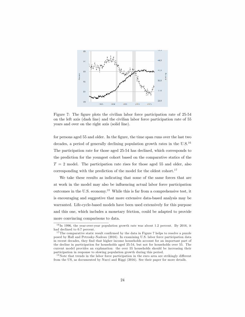
Figure 7: The figure plots the civilian labor force participation rate of 25-54on the left axis (dash line) and the civilian labor force participation rate of 55years and over on the right axis (solid line).

for persons aged 55 and older. In the figure, the time span runs over the last two

decades, a period of generally declining population growth rates in the U.S.16

The participation rate for those aged 25-54 has declined, which corresponds to

the prediction for the youngest cohort based on the comparative statics of the

T = 2 model. The participation rate rises for those aged 55 and older, also

corresponding with the prediction of the model for the oldest cohort.17

We take these results as indicating that some of the same forces that are

at work in the model may also be influencing actual labor force participation

outcomes in the U.S. economy.18 While this is far from a comprehensive test, it

is encouraging and suggestive that more extensive data-based analysis may be

warranted. Life-cycle-based models have been used extensively for this purpose

and this one, which includes a monetary friction, could be adapted to provide

more convincing comparisons to data.

16 In 1996, the year-over-year population growth rate was about 1.2 percent. By 2016, ithad declined to 0.7 percent.17The comparative static result confirmed by the data in Figure 7 helps to resolve a puzzle

posed by Hall and Petrosky-Nadeau (2016). In examining U.S. labor force participation datain recent decades, they find that higher income households account for an important part ofthe decline in participation for households aged 25-54, but not for households over 55. Thecurrent model provides an explanation: the over 55 households should be increasing theirparticipation in response to slowing population growth during this period.18Note that trends in the labor force participation in the euro area are strikingly different

from the US, as documented by Nucci and Riggi (2016). See their paper for more details.

24

4 Conclusion

We have provided an analysis of a version of nominal GDP targeting as optimal

monetary policy in a model with a credit market friction (NSCNC) following

ABSS (2016). The extension here has been to add elastic labor supply as well

as population growth. We wanted to study the case of elastic labor supply

because, by giving households another margin on which to adjust to shocks, it

is possible that nominal GDP targeting would no longer characterize optimal

monetary policy as it does in ABSS (2016).

Our main result is that optimal monetary policy is still characterized by a

version of nominal GDP targeting even in the expanded setting of this paper.

This result could be characterized as a “divine coincidence”result– by provid-

ing the optimal monetary policy through countercyclical price level movements,

the monetary authority also allows the heterogeneous households to make op-

timal labor supply decisions. Those decisions do not depend on the aggregate

productivity shock in the model and are instead demographically based. We

have related these findings to some current issues in U.S. monetary policy.

The life cycle framework used here is quite flexible and has been widely used

in the literature to study income and wealth inequality, labor supply issues,

as well as consumption and saving. The highly stylized version proposed here

and in ABSS (2016) has an important role for monetary policy via a credit

market friction as the centerpiece of the theory, similar to Sheedy (2014) and

Koenig (2013). While the stylized version provides a lot of clarity as to what

is going on in the model and the role for monetary policy, we also think the

model is flexible enough to be taken to the data in a more comprehensive way

in future versions. In addition, we think that the results here could be expanded

to include additional assets, like capital, and also to include idiosyncratic labor

income risk, as suggested in Werning (2014).

References

[1] Aaronson, S., B. Fallick, A. Figura, J. Pingle, and W. Wascher. 2006.

“The Recent Decline in Labor Force Participation and Its Implications for

25

Potential Labor Supply.”Brookings Papers on Economic Activity, Spring,

69-154.

[2] Aaronson, S., T. Cajner, B. Fallick, F. Galbis-Reig, C. Smith, and W.

Wascher. 2014. “Labor Force Participation: Recent Developments and Fu-

ture Prospects.”Brookings Papers on Economic Activity, Fall, 197-255.

[3] Aksoy, Y., R. P. Smith, T. Grasl, and H. Basso. 2015. “Demographic Struc-

ture and Macroeconomic Trends.”Working paper, Banco de España.

[4] Alvarez, F., and F. Lippi. 2014. “Persistent Liquidity Effect and Long run

money demand.” American Economic Journal: Macroeconomics, 6, 71—

107.

[5] Azariadis, C., J. Bullard, A. Singh, and J. Suda. 2016. “Incomplete Credit

Markets and Monetary Policy.”Working paper, Federal Reserve Bank of

St. Louis.

[6] Blanchard, O., and J. Gali. 2010. “Labor Markets and Monetary Policy: A

New-Keynesian Model with Unemployment.”American Economic Journal:

Macroeconomics, 2, 1—30.

[7] Bullard, J. 2014. “The Rise and Fall of Labor Force Participation in the

U.S." Federal Reserve Bank of St. Louis Review, 96, 1-12

[8] Bullard, J. 2014. “Discussion of ‘Debt and Incomplete Financial Markets’

by Kevin Sheedy.”Brookings Papers on Economic Activity, Spring, 362-

368.

[9] Chari, V., and P. Kehoe. 1999. “Optimal Fiscal and Monetary Policy.”In J.

Taylor and M. Woodford, eds., Handbook of Monetary Economics, Volume

1C, 26: 1671-1745. Elsevier.

[10] Daly, M., E. Elias, B. Hobijn, and Ò. Jordà. 2012. “Will the Jobless Rate

Drop Take a Break?” Federal Reserve Bank of San Francisco Economic

Letter .

26

[11] Diamond, P. 1965. “National Debt in a Neoclassical Growth Model.”Amer-

ican Economic Review, 55, 1126-1150.

[12] Erceg, C., and A. Levin. 2014. “Labor Force Participation and Monetary

Policy in the Wake of the Great Recession.”Journal of Money, Credit, and

Banking, Supplement, 46, 3-49.

[13] Eggertsson, G. B., and N. R. Mehrotra. 2015. “A Model of Secular Stag-

nation.”Working paper # 20574, National Bureau of Economic Research,

Inc.

[14] Fair, R., and K. Dominguez. 1991. “Effects of the Changing US Age Dis-

tribution on Macroeconomic Equations.”American Economic Review, 81,

1276—1294.

[15] Feng, Z., and M. Hoelle. 2017. “Indeterminacy in Stochastic Overlapping

Generations Models: Real Effects in the Long Run.”Economic Theory, 63,

559-85.

[16] Hall, R., and N. Petrosky-Nadeau. 2016. “Changes in Labor Participation

and Household Income.”Federal Reserve Bank of San Francisco Economic

Letter.

[17] Hotchkiss, J., and F. Rios-Avila. 2013. “Identifying Factors behind the

Decline in the Labor Force Participation Rate.”Business and Economic

Research, 3, 257—75.

[18] Koenig, E. 2013. “Like a Good Neighbor: Monetary Policy, Financial Sta-

bility, and the Distribution of Risk.”International Journal of Central Bank-

ing 9, 57—82.

[19] Krueger, A. 2016. “Where Have all the Workers Gone?”Working paper,

Princeton.

[20] Miles, D. 1999. “Modelling the Impact of Demographic Change upon the

Economy.”Economic Journal, 109, 1—36.

27

[21] Nucci, F., and M. Riggi. 2016. "Labor Force Participation, Wage Rigidities,

and Inflation." Working paper, Banca D’Italia.

[22] Sheedy, K. 2014. “Debt and Incomplete Financial Markets: A Case for

Nominal GDP Targeting.”Brookings Papers on Economic Activity, Spring,

301-361.

[23] Sterk, V., and S. Tenreyro. 2016. ”The Transmission of Monetary Policy

through Redistributions and Durable Purchases.”Working Paper # 1601,

Council on Economic Policies.

[24] Van Zandweghe, W. 2012. “Interpreting the Recent Decline in Labor Force

Participation.” Economic Review, Federal Reserve Bank of Kansas City,

5—34.

[25] Werning, I. 2014. “Discussion of ‘Debt and Incomplete Financial Markets’

by Kevin Sheedy.”Brookings Papers on Economic Activity, Spring, 368-

373.

[26] Woodford, M. 2003. Interest and Prices. Princeton University Press.

5 Appendix

5.1 Details of model solution

The model features heterogeneous households and an aggregate shock, so that

the evolution of the asset-holding distribution in the economy is part of the

description of the equilibrium. This would normally require numerical compu-

tation. However, symmetry, log preferences, and other simplifying assumptions

allow solution by “pencil and paper”methods. In this appendix we outline this

solution in some detail. A key feature of the solution is that the asset-holding

distribution will be linear in the current real wage w (t) , and so will simply shift

up and down with changes in w (t) . Another key feature of the solution will be

that the stochastic real rate of return on asset-holding will be equal to the sto-

chastic real output growth rate period-by-period. We do not claim uniqueness

28

of this equilibrium, but we regard the equilibrium we isolate as a natural focal

point for this analysis.19

We guess-and-verify a solution given a particular price rule for P employed

by the monetary authority.

(1) We first propose the state-contingent policy rule for the price level P.

(2a) We then solve the household problem under the proposed policy and

determine their state-contingent plan for consumption and non-state contingent

plan for leisure.

(2b) Step 2a also applies for all other households entering the economy at

earlier dates with shorter horizons and asset holdings from the previous period.

We show how these households will adjust their asset holdings as the real wage

evolves.

(3) We then establish that per capita consumption is equal, the optimal

“equity share”contract.

(4) Finally we verify that under the proposed policy rule and the derived

household behavior, the loan market clearing condition is satisfied. This estab-

lishes the equilibrium in the credit sector of the economy.

We will assume interior solutions and verify later.

Step 1. The household entering the economy at date t faces uncertainty

about income over their life cycle because it does not know what the real wage

level is going to be in the future. The proposed state-contingent policy rule

eliminates this uncertainty and is given by

P (t+ 1) =Rn (t, t+ 1)

ψλr (t, t+ 1)P (t) (35)

for all t, with P (0) > 0.

Step 2a.

First consider households entering the economy at date t. We use

max{ct(t+s),lt(t+s)}Ts=0

Et[

T∑s=0

[η ln ct (t+ s) + (1− η) ln `t (t+ s)] (36)

subject to life-time budget constraint

19See Feng and Hoelle (2017) for a recent discussion and analysis. Typical quantitative-theoretic applications in the area of stochastic OLG would be unable to address the issuesbrought out by the Feng and Hoelle (2017) analysis.

29

T∑s=0

P (t+ s)

P (t)

ct (t+ s)s−1∏j=0

Rn (t+ j, t+ j + 1)

≤T∑s=0

P (t+ s)

P (t)

esw (t+ s) (1− `t (t+ s))s−1∏j=0

Rn (t+ j, t+ j + 1)

.

(37)

Substitution of the policy rule into the budget constraint for these households

yields

T∑s=0

ct (t+ s)

ψss−1∏j=0

λr (t+ j, t+ j + 1)

≤ w(t)T∑s=0

ψ−ses (1− `t (t+ s)) . (38)

Because w (t) is known by the household at the time when this problem is solved,

the uncertainty about future income has been eliminated by the state-contingent

policy. The household then solves this problem where µ is the multiplier on the

life-time budget constraint. The following sequence of first order conditions for

s = 0, 1, ..., T with respect to consumption are

η

ct (t+ s)=

µ

ψss−1∏j=0

λr (t+ j, t+ j + 1)

(39)

which implies

ct (t+ s) =

ψs s−1∏j=0

λr (t+ j, t+ j + 1)

ct (t) (40)

The following sequence of first order conditions for s = 0, 1, ..., T with respect

to ` are1− η

`t (t+ s)= µw (t)ψ−ses (41)

Using the FOC for first period consumption to substitute out µ gives the fol-

lowing choices for leisure for s = 0, 1, ..., T

`t (t+ s) =1− ηη

ct (t)

w (t)ψ−ses(42)

30

We can then substitute back into the budget constraint, which is

(T + 1)ct (t) ≤ w(t)T∑s=0

ψ−ses (1− `t (t+ s)) . (43)

Substituting for leisure gives

(T + 1)ct (t) ≤ w (t)T∑s=0

ψ−ses

(1− η

1− ηct (t)

w (t)ψ−ses

)(44)

This is

(T + 1)η

ηct (t) +

1− ηη

ct (t) = w (t)

T∑s=0

ψ−ses (45)

or

ct (t) = w (t)η

T + 1

T∑j=0

ψ−jej (46)

We conclude that the choice for ct (t) , first period consumption depends on

today’s wage w (t) alone. The household has a state-contingent consumption

plan for the future. It is to consume

ct (t+ s) =

ψs s−1∏j=0

λr (t+ j, t+ j + 1)

ct (t) . (47)

depending on the realizations of future shocks to the TFP growth rate λ.

The amount of leisure chosen at date t and in the future depends on where

they are in the life cycle. They are given by

`t (t+ s) =

(1− ηT + 1

)(1

ψ−ses

) T∑j=0

ψ−jej . (48)

If η = 1 the household will choose no leisure. If η → 0 and e0 = eT are

small enough, then `t (t) and `t (t+ T ) could be larger than one, meaning the

households would supply no labor on those dates. This would violate our inte-

rior solution assumption. We assume e0 = eT � 0 and η suffi ciently large to

maintain interior leisure choices.

This household will carry some nominal asset position into the next period.

31

The date t real value of this position is given by

at (t)

P (t)= e0 [1− `t (t)]w (t)− ct (t) (49)

= e0

1−1− ηT + 1

T∑j=0

ψ−jej

e0

w (t)−η

T + 1w (t)

T∑j=0

ψ−jej

(50)

= w (t)

e0 + η − 1T + 1

T∑j=0

ψ−jej

− η

T + 1

T∑j=0

ψ−jej

(51)

= w (t)

e0 − 1

T + 1

T∑j=0

ψ−jej

. (52)

Step 2b.

There are also households that entered the economy at date t−1, t−2, · · · , t−T that would solve a similar problem. These households would have brought

nominal asset holdings at−1 (t− 1) , at−2 (t− 1) , · · · , at−T (t) , respectively, intothe current period, and have a shorter remaining horizon in their life cycle. Here

we will show the solution to a household problem for a household that entered

the economy at date t−1. In particular, we will show that asset holdings at−1 (t)continues to be linear in the current real wage w (t) .We will then infer solutions

for all of the other household problems for households entering the economy at

dates t− 2, · · · , t− T .The household entering the economy at date t−1 solve this problem at date

t :

max{ct−1(t+s−1),lt−1(t+s−1)}Ts=1

Et[

T∑s=1

[η ln ct−1 (t+ s− 1) + (1− η) ln `t−1 (t+ s− 1)]

subject to life-time budget constraint

32

T∑s=1

P (t+ s− 1)

P (t)

ct−1 (t+ s− 1)s−1∏j=0

Rn (t+ j, t+ j + 1)

≤T∑s=1

P (t+ s− 1)

P (t)

esw (t+ s) (1− `t (t+ s))s−1∏j=0

Rn (t+ j, t+ j + 1)

+Rn (t− 1, t) at−1 (t− 1)

P (t)..

(53)

In this “remaining lifetime”budget constraint, we can see from section 2a

above what the (nominal) value of at−1 (t− 1) must have been from last period,namely

at−1 (t− 1) = P (t− 1)w (t− 1)

e0 − 1

T + 1

T∑j=0

ψ−jej

. (54)

We can therefore find the value of Rn (t− 1, t) at−1 (t− 1) as

Rn (t− 1, t) at−1 (t− 1) = Rn (t− 1, t)P (t− 1)w (t− 1)

e0 − 1

T + 1

T∑j=0

ψ−jej

.(55)

We can use the policy rule P (t) = Rn(t−1,t)ψλr(t−1,t)P (t− 1) and the law of motion for

w (t) to simplify the RHS as

= Rn (t− 1, t) P (t)ψλr (t− 1, t)

Rn (t− 1, t)w (t)

λr (t− 1, t)

e0 − 1

T + 1

T∑j=0

ψ−jej

(56)= ψP (t)w (t)

e0 − 1

T + 1

T∑j=0

ψ−jej

. (57)

Therefore the entire real-valued term is given by

Rn (t− 1, t) at−1 (t− 1)P (t)

= ψw (t)

e0 − 1

T + 1

T∑j=0

ψ−jej

(58)

= w (t)

T

T + 1ψe0 −

1

T + 1

T∑j=1

ψ−(j−1)ej

.(59)33

Since w (t) and P (t) are known at date t when the consumption-saving decision

is made, this is a nonstochastic object. It is linear in w (t) . It enters in lump-sum

fashion in the budget constraint and so does not affect the first order conditions.

We now substitute the policy rule into the rest of the budget constraint to

obtain

T∑s=1

ct−1 (t+ s− 1)

ψs−1s−1∏j=0

λr (t+ j, t+ j + 1)

≤ w(t)

T∑s=1

ψ−(s−1)es (1− `t−1 (t+ s− 1)) +T

T + 1ψe0 −

1

T + 1

T∑j=1

ψ−(j−1)ej

.

(60)

As previously there is no income uncertainty for this household.

Let’s now turn to the FOC for this problem. We have for s = 1, 1, ..., T with

respect to consumption are

η

ct−1 (t+ s− 1)=

µ

ψs−1s−1∏j=0

λr (t+ j, t+ j + 1)

(61)

which implies

ct−1 (t+ s) =

ψs s∏j=0

λr (t+ j, t+ j + 1)

ct−1 (t) (62)

The following sequence of first order conditions for s = 1, ..., T with respect to

` are1− η

`t−1 (t+ s− 1)= µw (t)ψ−(s−1)es (63)

We combine each of these with the corresponding FOC for consumption to give

the following choices for leisure for s = 1, ..., T

`t−1 (t+ s− 1) =1− ηη

ct−1 (t)

w (t)ψ−(s−1)es(64)

We can now substitute back into the "remaining life" budget constraint.

This yields

34

Tct−1 (t) ≤ w(t)

T∑s=1

ψ−(s−1)es

(1− 1− η

η

ct−1 (t)

w (t)ψ−(s−1)es

)+

T

T + 1ψe0 −

1

T + 1

T∑j=1

ψ−(j−1)ej

(65)

Tη

ηct−1 (t)+T

1− ηη

ct−1 (t) = w (t)

T∑s=1

ψ−(s−1)es+w (t)

T

T + 1ψe0 −

1

T + 1

T∑j=1

ψ−(j−1)ej

(66)

ct−1 (t) = w (t)η

T + 1

ψe0 + T∑j=1

ψ−(j−1)ej

. (67)

This is linear in w (t) . This household would then have a desired asset position:

at−1 (t)

P (t)= e1w (t) (1− `t−1 (t))− ct−1 (t) +

Rn (t− 1, t) at−1 (t− 1)P (t)

(68)

= e1w (t)

[1 +

η − 1η

ct−1 (t)

e1w (t)

]− η

ηct−1 (t) + w (t)

T

T + 1ψe0 −

1

T + 1

T∑j=1

ψ−(j−1)ej

,= e1w (t)−

1

ηct−1 (t) + w (t)

T

T + 1ψe0 −

1

T + 1

T∑j=1

ψ−(j−1)ej

,= e1w (t)−

1

ηw (t)

η

T + 1

[ψe0 +

T∑s=1

ψ−(s−1)es

]+ w (t)

T

T + 1ψe0 −

1

T + 1

T∑j=1

ψ−(j−1)ej

,= w (t)

e1 − 1

T + 1

[ψe0 +

T∑s=1

ψ−(s−1)es

]+

T

T + 1ψe0 −

1

T + 1

T∑j=1

ψ−(j−1)ej

= w (t)

1

T + 1

ψe0 + e1 − T T∑j=2

ψ−(j−1)ej

.For all other households at date t who entered the economy at date t − 2, t −3, ..t− T, consumption and assets at date t will also be linear in w(t).Step 3.

35

We now wish to show that per capita consumption is equalized among house-

holds. The consumption amounts are

ct (t) = w (t)η

T + 1

T∑j=0

ψ−jej, (69)

ct−1 (t) = w (t)η

T + 1

ψe0 + T∑j=1

ψ−(j−1)ej

, (70)

ct−2 (t) = w (t)η

T + 1

ψ2e0 + ψe1 + T∑j=2

ψ−(j−2)ej

..... (71)

The cohort entering the economy at date t − 2 is smaller than the cohort thatentered the economy at date t by a factor of ψ−2, and the cohort entering the

economy at date t−1 is smaller by a factor of ψ−1.Multiplying through by thesefactors indicates that per capita consumption is equalized under the proposed

policy rule for P.

Step 4.

Let’s denote the government-issued nominal debt byB (t) . It is issued promis-

ing a non-state contingent nominal rate of return. The difference between

the privately-issued nominal debt and the aggregate nominal asset positions

of households must be the government-issued nominal debt. The equilibrium

condition is therefore

B (t) =

T−1∑s=0

nt−sat−s (t) (72)

B (t) = Rn (t− 1, t)B (t− 1) . (73)

The second part of this can be viewed as a bond issuance rule. Today’s bond

issuance must be just enough to pay principle and interest on previous bond

issuance.

36

The equilibrium conditions can be combined to yield

T−1∑s=0

nt−sat−s (t) = Rn (t− 1, t)[T∑s=1

nt−sat−s (t− 1)]

(74)

nt

[T−1∑s=0

ψ−sat−s

]= Rn (t− 1, t)

[nt−1

[T∑s=1

ψ−(s−1)at−s (t− 1)]]

(75)

T−1∑s=0

ψ−sat−s = Rn (t− 1, t)[T∑s=1

ψ−sat−s (t− 1)]

(76)

Substituting out the (nominal) asset positions and noting that

w (t)P (t)

w (t− 1)P (t− 1) = λr (t− 1, t) Rn (t− 1, t)

λr (t− 1, t)ψ =Rn (t− 1, t)

ψ, (77)

the bond issuance rule is satisfied in an equilibrium in which the real rate of

interest is equal to the real rate of output growth.

37