nomen_oseghale thesis (e.o)

Ehinomhen (Nomen) Oseghale: E-bus: HVAC optimisation of an urban transport vehicle: a CFD model for the evaluation of internal energy loss

1 | P a g e

E-bus: HVAC optimisation of an urban transport vehicle: a CFD model for the evaluation of internal energy loss Author: Ehinomhen (Nomen) Oseghale

School of Aerospace, Mechanical and Manufacturing Engineering, RMIT University PO Box 71, Bundoora, Victoria

3083, Australia

Email address:

[email protected] {Ehinomhen (Nomen) Oseghale}

To cite this article:

Ehinomhen (Nomen) Oseghale, E-bus: HVAC optimisation of an urban transport vehicle: a CFD model for the

evaluation of internal energy loss.

Abstract: The main aim of this work is to minimize the indoor energy gain/loss in an urban transit electric bus.

In summer the battery powered electric bus uses 13kW of total load to run the HVAC system. Therefore reducing the

total energy loss will result in reduction of the total energy used to run the ventilation and air-condition system, also

reduce the bus battery size and save money. This article reports the results of CFD simulation of the bus at steady

state, when the doors are open (transient) and proposed solution to reduce the volume of hot air going into the bus.

CATIA 3D CAD software was used to develop an accurate three-dimensional bus model. Air flow analysis was carried

out using ANSYS CFD-CFX ©. The three main components within the bus structure are ventilation (outlet), diffuser

(inlet), door (opening) and Outside world. The steady state temperature is been simulated and the result is justified,

it takes 4 minutes to get the bus to a steady state temperature (30C to 20C). To validate the transient simulation, an

outside world is created. The outside world is attached to the bus on ANSY CFX and has a constant temperature of

40C and constant 5m/s wind. It was found that more energy goes into the bus when the wind direction is from the

front of the bus. Ventilation and diffusers work together as this provides equilibrium of pressure inside the bus, to

achieve an equilibrium state the inlet mass flow rate was set as 1.11kg/s and outlet vent pressure is 0Pa. Two

solutions were tested, the solutions were applying blower on top of door and turning off the RHS diffuser while

doubling the pressure for the LHS diffusers. This solution is was successful to an extent. The new proposed solution is

to add ‘Mechanical curved pads to outside the doors’; this solution is potentially going to produce more beneficial

results. The plan is to create curved pads across the door (Y direction); these curved pads will open when the door is

open. So when the air blows, the air curves over the curved pads across the door and potentially deflects the air

from going into the bus through the doors. This new proposed solution is been designed and tested.

Keywords: Diffuser, CFD, ANSYS, CFX, CATIA, CAD, Bus, Energy, Door, HVAC, Airflow, Analysis

1. Introduction In the world today auto companies are

pushing to electrify public buses. A major

challenge is minimizing the total energy

consumption of the HVAC systems in these buses.

In large cities such as Queensland there is a high

demand for lithium ion battery powered electric

busses due to its incredible low energy density

compared to diesel busses. Battery powered

electric bus is an evolutional technology and is still

being improved to suit this day and age. E-bus is a

mailto:[email protected]


2 | P a g e

bus that is driven by an electric motor and two

tonne battery and its’ energy is obtained as does

by an electric car. Electric busses are of vital

importance socially and economically, its

importance affects public transport uses globally.

The idea of energy loss in public transport arises

from the somewhat frequent door opening of

these busses. The internal temperature humidity

conditions are an important factor for the

comfort, health and safety of passengers and

drivers. To recreate this pattern it is a must that

the physical aspects are accurate. Air flows from

a region at high pressure to a region at low

pressure. As long as there is a pressure difference,

there is an air flow and in this case, the bus

interior is at a low pressure and the exterior is at a

high pressure (initially). Air flows in through the

diffusers. As air molecules accumulate inside the

bus, the pressure inside increases at a certain

rate. At one instant, equilibrium is reached and

the air stops flowing. Now, the air molecules can

only flow out of the bus if the pressure outside

drops to a low value such that, there is a pressure

difference. In this case, the interior is at a high

pressure when compared to the exterior. It's only

in this case that the air molecules flow out of the

bus. For this reasons the automotive industry has

developed ways to model the internal of the bus

and door structure to keep the loss of internal

energy to a minimum. If this goal is achieved, then

the energy loss actual value will be valid.

In this experiment, in order make adequate

progression, with the aid of CFD several

computational simulation scenarios will be carried

out to determine the airflow changes in the bus

internal.

3. CFD model Simulations are performed with the commercial

CFD software CFX-PRE [3]. Although this software

is used because it provides state of the art grid

generation and flow modelling capabilities,

comparable results could be obtained with any of

the many similar numerical commercial models

available. Three different representations of the

fluid flow in the room are used: laminar flow,

turbulent flow using the standard k–ε turbulence

model, and turbulent flow using the RNG k–ε

turbulence model. In a relatively recent study,

Chen [4] compared the performance of five

different models for simulating simple indoor air

flows and found that the standard and RNG k–ε

predicted actual flow patterns best. The RNG

model was found to perform slightly better than

the standard model in some situations [5] and [7].

The validity of the RNG k–ε model is not yet

assured, however, due to its entirely theoretical

development and lack of widespread application

[8] and [11], but there is particular interest in its

performance with complex indoor air flows.

2. Numerical Analysis The mathematical model, implemented for the

optimization of the air distribution system, inside

the compartment of a bus, was built using CFD

numerical analysis software (CFX-PRE ©).

The CFD, Computational Fluid Dynamics,

software identifies the method which, through

numerical algorithms, leads to the solution of the

equations which could be the laminar, or a fluid’s

turbulent motion and of the related thermo-

dynamic processes within a specified geometry.

The 3 contributors to the bus internal heat gain

are;

Radiation (1kW/m^2 @ 12 noon in

summer)

Convection

Conduction

3. Existing situation Analysis To make adequate progress towards achieving the

aims and objectives, certain adequate

experiments have to be taken and resulting data

must be analysed to full potential. Below is the 2

main simulations done to make adequate

progress towards the aim and objectives.


3 | P a g e

Scenario 1: Internal temperature at

steady state

Scenario 2: Air mixing when door is open

The implementation of a CFD code provides

project validation, with low economic and time

requirements. The comfort can thus be foreseen,

building guidelines which are mostly useful in the

early stages of the system designation, enhancing

the reduction in energy consumption and

improving people‘s wellbeing. The numerical

model of the thermo-fluid dynamic phenomenon

has been carried out on a continuous model.

The governing equations for the indoor air

system are the mass conservation equation and

the Reynolds-averaged Navier–Stokes equations

for three-dimensional fluid flow. In the

simulations, three mathematical representations

are used to describe the air flow in the room.

During experimentation It was assumed that the

indoor flow is turbulent, this resulted in using a

standard k–ε turbulence model. [1,2]

2.1 Boundary conditions and flow

properties

Boundary conditions are necessary; it is used to

specify the value that a certain solution needs to

take along the boundary of the geometry domain.

In the case of the geometry used for the

experiment, below are the appropriate boundary

conditions used.

Inlet (Diffuser)

Outlet (Vent)

Door (Front & Rear)

Walls

Windows

2.1.1 CFX setup

Before running the simulation, several important

steps have to be taken. In order for the simulation

solution to produce accurate results the below

conditions has to be set to suit the problem

outcome.

Gravity

Energy (ON)

Viscous

Material air (ideal gas)

Air buoyancy density

Diffuser mass flow rate

Ventilation pressure

Initial bus pressure

Bodywork (Fibre glass)

Windows (Glass windows)

General geometry operation condition

Boundary conditions

Solution initialization (Initial conditions at

time=0)

Output request

2.2 Test Environment

There are 2 different geometries, one represents

the bus the other represents the outside world.

To replicate the best results we need to develop

an appropriate geometry/s. In this case our

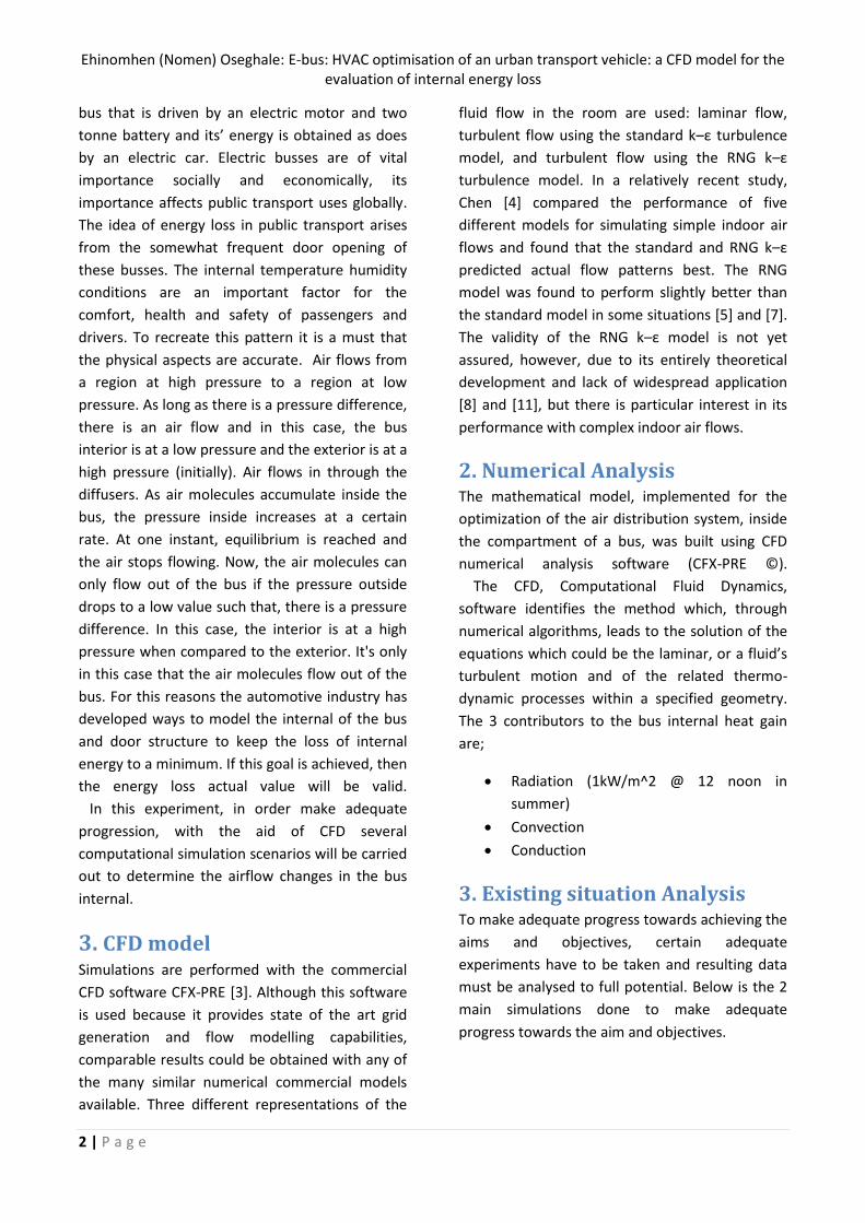
geometry is a 12.5 meter long bus. Its dimensions

are listed below;

Height – 2.61 m

Width (Extrusion) – 2.8 m

Length – 12.50 m

Fig 1: Model bus top view

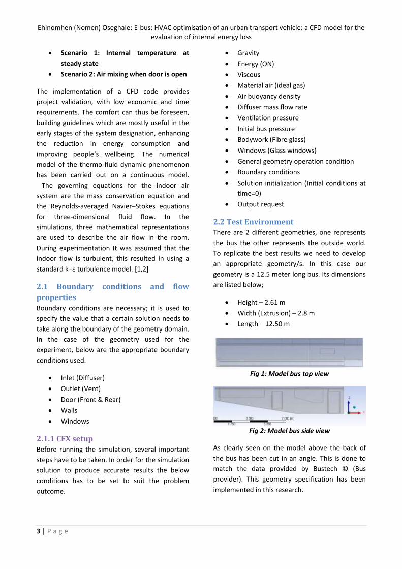
Fig 2: Model bus side view

As clearly seen on the model above the back of

the bus has been cut in an angle. This is done to

match the data provided by Bustech © (Bus

provider). This geometry specification has been

implemented in this research.


4 | P a g e

Fig 3: Model bus door view

Fig 4: Model bus isometric view

Fig 5: Model bus isometric view

A new addition is introduced to the geometries. In

order to have an accurate result we need to

attach an outside geometry to the bus, with

appropriate spacing between both geometries.

We need to do this in order for the software to

specify what conditions are outside. This will

result in an accurate solution when the bus doors

are open. The outside world has a constant

temperature of 40C and 5m/s wind in X and Y

directions in two separate scenarios.

Outside geometry dimensions shown below;

Height – 20.0 m

Width (Extrusion) – 22.0 m

Length – 40.0 m

Fig 6: Bus and Outside geometries

Fig 6.1: Bus and Outside geometries

In fluid mechanics investigations, sub-scale

models are often used to reduce the cost and

time associated with full-scale systems. In this

experiment full scale model is used to generate

the most accurate result possible matching the

actual situation inside the real life bus. Air flow

data is taken in a full-scale model bus passenger

compartment, which are relatively the exact same

dimensions, curves, edges and placements of

partitions etc. of a typical full-size bus indoor

space. The full scale model is needed so that an

actual solution can be provided to clients

(BUSTECH) after thorough investigation has been

carried out.

In this study, although there is no heating

cooling by the ventilation air, there are several

heating sources inside and outside the bus. Due to

the complications of external heat sources the

most important dimensionless parameter to be

aware of it Reynold number and buoyancy. In

most situations, buoyancy effects from heating

loads influence the structure of the air flow and


5 | P a g e

must be included, such effects are in this study

when dealing with outside air temperature, for

the purpose of accuracy and simplicity during the

simulation buoyancy was set to 1.2kg/m3 and

radiation heating source was turned off.

The sub-scale model room, as shown in Fig. 1,2,3

is made from fibre glass and has three plane glass

windows which provide adequate optical access;

the bus is 12.5m long, 2.4 m wide, and 2.8 m tall.

Four times 9 width 1.0 m long single inlet, 2.3 m

by 0.46 m outlet vent, both on the bus ceiling,

supply and remove ventilation air, windows on

both sides of the bus and a double door passenger

front door sitting at 1.2 m in width, height at 2.12

m and 3.5 m spacing from the front edge.

2.3 Meshing Before ANSYS CFX can calculate for a solution, we

need to mesh the geometry so the boundary

condition can act as expected. The boundary

conditions needs less mesh element size in order

for the results to be much more accurate. In other

words the finer the mesh the more accurate the

results. In this case a fine quality mesh was used.

Fig 7: Mesh door view

Fig 8: Mesh side view

Fig 9: Mesh top view

Fig 9.1: Mesh top view (Bus and Outside)

Fig 9.2: Outside inlet 5m/s wind

As seen on fig 6, 7, 8 the diffusers, Doors, inside

bus partitions, Vent and body have been sized

appropriately. Re-sizing these portions result in a

much more accurate simulation results and

airflow.

2.4 Numerical solution procedure

For the model bus, using the ventilation

component constant flow rate of 4800L/s, and the

air buoyancy of 1.2kg/m3 therefore it requires an

inlet mass-flow rate of 1.1 kg/s, the inlet contains

a disturbed turbulent flow. The inlet section is

long enough for the boundary layers to converge,

so the majority of the inlet air velocity profile is

that of turbulent plug flow. The high mass-flow

rate makes the system essentially less sensitive to

small disturbances and thermal gradients that are

assumed to be negligible in the numerical

simulation. The fluctuations of temperature and

pressure in the inlet section are very small; the

inlet is built to behave like a jet like airflow.

The vent pressure was set as 0 Pa, initial

pressure is set to 101325 Pa this will make sure

there is equilibrium pressure in the bus at all

times. Windows are set as fiberglass with a heat

transfer coefficient of 0.96Wm^-2K^-1.

The door settings is a grey area that will be

fixed, the proposed solution for this is to create an

external geometry.

The high sensitivity to upstream disturbances

requires that the pressure regulation and

upstream conditioning of the inlet be closely

monitored. A bypass flow meter helps maintain a


6 | P a g e

constant velocity and minimize pressure

perturbations. This bypass flow meter hasn’t been

created yet in this experiment, this could be the

cause of the inaccuracies. For the purpose of this

experiment the initial temperature is set to 30C

while the outside temperature is 40C

3. Results for Existing situation

Analysis In this work, we set out several goals/objectives.

The passenger comfort and energy change is

analysed when the door is closed and when its

open. The thermo-hygrometric changes are also

investigated, as transient temperature and air

speed gradients, related to the bus stop with open

doors. The opening and closing doors phase

usually lasts for 20-30 seconds and substantially

change the internal thermo-fluid dynamic

conditions by creating strong air speed and

temperature gradients [1]. The passenger comfort

is lost especially in some areas of the vehicle

compartment [1]. Referring to the main aim which

is optimizing the HVAC system, 3 different

solutions have been presented and is still ongoing

testing. Firstly we accomplished a steady state

temperature, from initial temperature of 30C to a

steady state temperature of 20C in a total of 3.5

minutes.

Secondly, we analyse the change in

internal energy when the bus door is open. To do

this the outside boundary conditions and

temperature were set. The constant temperature

is 40C; the temperature was used to represent the

test area in summer (Queensland Australia).

3.1 Scenario 1: Internal temperature at

steady state (Door closed)

Firstly an internal steady state temperature was

calculated and analysed (temperature of bus

internal at steady state (To)). In this case the aim

is to monitor the change in temperature inside

the geometry after X-number of seconds and

when the temperature reached a steady state the

simulation is stopped. In this set-up it is important

to replicate a real life air conditioning system, as p

[the specified total pressure of the air dispensing

from the diffusers should equal the total pressure

of air been extracted by the ventilation system

{Pin = Pout}.

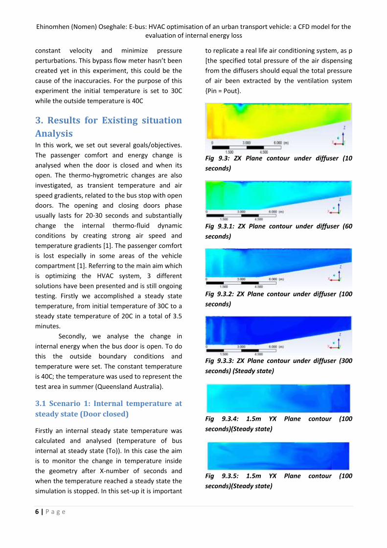
Fig 9.3: ZX Plane contour under diffuser (10

seconds)

Fig 9.3.1: ZX Plane contour under diffuser (60

seconds)


seconds)


seconds) (Steady state)

Fig 9.3.4: 1.5m YX Plane contour (100

seconds)(Steady state)

Fig 9.3.5: 1.5m YX Plane contour (100

seconds)(Steady state)


7 | P a g e

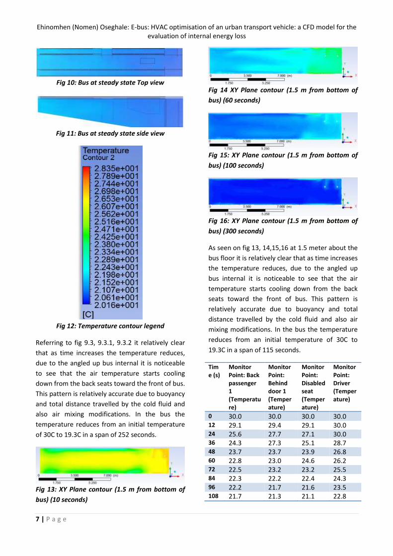
Fig 10: Bus at steady state Top view

Fig 11: Bus at steady state side view

Fig 12: Temperature contour legend

Referring to fig 9.3, 9.3.1, 9.3.2 it relatively clear

that as time increases the temperature reduces,

due to the angled up bus internal it is noticeable

to see that the air temperature starts cooling

down from the back seats toward the front of bus.

This pattern is relatively accurate due to buoyancy

and total distance travelled by the cold fluid and

also air mixing modifications. In the bus the

temperature reduces from an initial temperature

of 30C to 19.3C in a span of 252 seconds.

Fig 13: XY Plane contour (1.5 m from bottom of

bus) (10 seconds)

Fig 14 XY Plane contour (1.5 m from bottom of

bus) (60 seconds)


bus) (100 seconds)


bus) (300 seconds)

As seen on fig 13, 14,15,16 at 1.5 meter about the

bus floor it is relatively clear that as time increases

the temperature reduces, due to the angled up

bus internal it is noticeable to see that the air

temperature starts cooling down from the back

seats toward the front of bus. This pattern is

relatively accurate due to buoyancy and total

distance travelled by the cold fluid and also air

mixing modifications. In the bus the temperature

reduces from an initial temperature of 30C to

19.3C in a span of 115 seconds.

Time (s)

Monitor Point: Back passenger 1 (Temperature)

Monitor Point: Behind door 1 (Temperature)

Monitor Point: Disabled seat (Temperature)

Monitor Point: Driver (Temperature)

0 30.0 30.0 30.0 30.0 12 29.1 29.4 29.1 30.0 24 25.6 27.7 27.1 30.0 36 24.3 27.3 25.1 28.7 48 23.7 23.7 23.9 26.8 60 22.8 23.0 24.6 26.2 72 22.5 23.2 23.2 25.5 84 22.3 22.2 22.4 24.3 96 22.2 21.7 21.6 23.5 108 21.7 21.3 21.1 22.8


8 | P a g e

120 21.3 21.4 20.9 22.5 132 21.4 21.0 20.7 22.0 144 21.3 20.5 20.5 21.6 156 21.0 20.4 20.4 21.2 168 20.9 20.4 20.3 20.9 180 20.7 20.5 20.1 20.8 192 20.7 20.4 20.1 20.8

204 20.7 20.2 20.2 20.6 216 20.6 20.2 20.2 20.5 228 20.6 20.3 20.1 20.5 240 20.5 20.2 20.1 20.4 252 20.4 20.2 20.1 20.4

Avg 22.4 22.4 22.3 23.6 Table 1: Test points temperature over time.

Graph 1: Test points temperature (C) over time (s).

The graph above shows a realistic trend in

temperature changes when the diffusers are

turned on. It can be seen that the max

temperature is 30C (initial), after 4 minutes the

bus reaches a minimum steady state temperature

of 20C.

Fig 17: Airflow streamline of inlet and outlet (AC

on) (1 second)


on)


on)

As seen on fig 17, 18, 19 the internal airflow

streamline shows the airflow movement and

change in temperature as it moves through the

bus towards the vent. This pattern is relatively

accurate as the diffuser cools the bus the vent

19.00

21.00

23.00

25.00

27.00

29.00

31.00

0 30 60 90 120 150 180 210 240

Tem

pe

ratu

re (

C)

STEADY STATE

Monitor Point:Back passenger 1(Temperature)

Monitor Point:Behind door 1(Temperature)

Monitor Point:Disabled seat(Temperature)

Monitor Point:Driver(Temperature)


9 | P a g e

sucks out air from the bus and keeps and

equilibrium pressure in the bus passenger cabinet

After thoroughly analysing all data it can be said

that the results and not fully accurate due to

reasons such as; To achieve a more improved

accurate result we, a series of two pressure

regulators should be set incrementally to ensure

that pressure perturbations do not propagate into

the experiment. The flow rate is controlled by a

needle valve, and the flow rate is adjusted until

1.11 kg/s is measured with the LDA system at the

centre of the inlet jet [3].

3.2 Scenario 2: Door Open (Transient

solution) In this case we introduce a new addition to the

geometry. In order to have an accurate result we

need to attach an outside geometry to the bus

geometry, with appropriate spacing between both

geometries. The door dimensions are standard

and its dimensions are shown below;

Fig 20: Bus door view

Front door:

h = 2122 mm

L = 1256 mm

Rear door:

h = 2122 mm

L = 870 mm

The aim here is to simulate the airflow inside the

bus when the door is open. To do this we need to

introduce an outside domain, this domain will act

as an outside. This means the door will act as a

real boundary condition, the bus door and the

outside geometry are attached using CGI

interface. The outside domain has a constant 40C.

The outside domain shown below;

Fig 21: Outside domain

3.2.1 Scenario 2: Air mixing when door is

open (Door open)

When the door is open several variables could

determine if the result will be accurate, such

variables includes;

Initial Internal pressure

Diffuser pressure

Outlet vent pressure

Door setting

Outside environment pressure

Taking all of the above into consideration, the

following results were simulated on ANSYS CFX ©

3.3 Door Open

Several variables needs to be considered when

the bus doors are open, and various boundary

conditions and initial conditions need to be set.

These variables include;

Test 1: Door Open wind in X-direction

Initial temperature inside bus – 20C

Initial temperature outside bus – 40C

Constant wind velocity and direction –

5m/s towards bus (X direction)

Bus inlet temperature – 20C (Constant)

Door open at– 5s

Door open total time – 75s (1.15 mins)


10 | P a g e

Fig 22: Door open top view(X direction)

Fig 23: Door open door view (after 3s) (X

direction)


direction)


direction)

Fig 26: Door open door view (after75s) (X

direction)

Fig 27: Door open top view (after75s) (X

direction)

Figure 22 clearly illustrates the top view of both

the bus and outside domains. It shows that the

outside has a constant 40C degree temperature.

Fig 23 After 3 seconds, it proves that the doors

and outside domains are in perfect sync; this can

be confirmed by looking at the hot air rise above

the colder air, therefore the hot air blows into the

bus through the top of the door and the cold air

escapes through the bottom, this validates the

laws of physics. The hot air has lower buoyancy

(1.12kgm3) while the cold air-conditioned air has

a buoyancy of 1.2kgm3. These buoyancy values

are not constant, the buoyancy value changes

with temperature. Figure 24 shows the

temperature contour the door after 9 seconds.

Figures 25, 26, & 27 shows that after 45 seconds

and 75 seconds respectively, the hot air goes into

the bus through the front door and the keep an

equilibrium pressure the air-conditioned air goes

out through the back door. Figures 28 & 29

displays streamlines at the bus doors, showing air

going in and out of the bus.

Fig 28: 1.5m XY Plane Door open top view (after

0s) (Wind X direction)







Figure 28 shows the bus at a height of 1.5 meters

from the top of bus at time 0 seconds (Door just

opens). Figure 29 clearly shows the results when

the bus doors are open, it can clearly be seen that

the air goes in through the front door at a higher


11 | P a g e

rate and velocity that the back door. Reason for

this is due to the fact that the vent is located close

to the front door. Therefore the air that goes into

the bus is relatively sucked through the vent to

keep an equilibrium pressure and stable

temperature inside the bus. Figure 30 & 31 shows

the progression of the airflow in respect to time

45 seconds and 75 seconds respectively.







Figure 32, 33 & 34 shows the bus at a height of

2.1 meters from the top of bus at time 9, 45 and

75 seconds respectively.

Time (s)

Back passenger (C)

Behind rear door (C)

Behind front door (C)

Disabled seat (C)

Driver (C)

Outside (C)

0 20.0 20.0 20.0 20.0 20.0 40.0 3 20.0 20.0 20.0 20.0 20.0 40.0 6 20.0 20.0 20.3 20.1 20.7 40.0 9 20.0 20.0 20.3 20.9 20.7 40.0

12 20.0 20.0 20.3 22.3 24.2 40.0 15 20.1 20.0 20.2 23.5 27.1 40.0 18 20.4 20.0 21.2 22.8 24.5 40.0 21 20.9 20.1 21.8 22.1 24.5 40.0 24 21.7 20.1 22.3 22.7 27.6 40.0 27 22.2 20.1 23.2 23.8 27.5 40.0 30 22.1 20.3 23.5 24.0 27.1 40.0 33 22.5 20.4 23.2 24.9 26.5 40.0 36 23.4 20.4 23.5 25.3 26.2 40.0 39 24.0 20.5 23.7 24.6 26.6 40.0 42 24.5 20.5 23.6 24.5 26.6 40.0 45 24.6 20.6 23.5 24.4 26.5 40.0 48 24.2 20.7 24.2 24.4 27.6 40.0 51 23.6 20.8 24.8 24.2 27.1 40.0 54 23.3 21.0 26.4 24.0 26.4 40.0 57 23.2 21.1 25.8 24.3 26.4 40.0 60 23.3 21.2 23.5 24.4 27.4 40.0 63 23.3 21.3 22.7 24.2 28.4 40.0 66 23.4 21.3 23.1 24.9 27.5 40.0 69 23.4 21.3 23.7 26.0 27.0 40.0 72 23.4 21.3 24.1 26.2 27.0 40.0 75 23.9 21.4 24.0 25.5 29.2 40.0

Avg 22.4 20.6 22.8 23.6 25.8 40.0 Table 2: Test points temperature over time when

door is open for 75 seconds (Wind in X-direction).


12 | P a g e


Table 2 shows that the driver hits a maximum

temperature of 29.9C at time 75 seconds. The

passenger behind the rear door has a record low

average temperature of 20.6C followed by the

back passenger 22.4C. The driver records the

highest temperature of 25.8C. This temperature

change inside the bus proves the fact that energy

is been lost and gained when the doors are open.

It also solidifies the outside domain working as

intended.

Test 2: Door Open wind in Y-direction

Initial temperature inside bus – 20C

Initial temperature outside bus – 40C

Constant wind velocity and direction –

5m/s towards bus (Y direction)

Bus inlet temperature – 20C (Constant)

Door open at– 5s

Door open total time – 75s (1.15 mins)

Fig 35: Door open door view (after 9s) (Y

direction)

Fig 36: Door open door view (after75s) (Y

direction)

Fig 37: Door open top view (after75s) (X

direction)

As seen on figures 35, 36 & 37 it can be seen

that the result’s looks as expected. At 9

seconds the hot 5m/s air will blow in through

the rear door that and the makes it way to

the front door where the vent is located.


0s) (Wind Y direction)

15.00

20.00

25.00

30.00

35.00

40.00

1 2 3 4 5 6 7 8 9 10 11 12 13 14 15 16 17 18 19 20 21 22 23 24 25 26

Tem

pe

ratu

re (C

)

AC ON Door Open (Wind from back) Monitor Point: Backpassenger 1 (Temperature)

Monitor Point: Backpassenger (Temperature)

Monitor Point: Behinddoor 2 (Temperature)

Monitor Point: Behindfront door (Temperature)

Monitor Point: Disabledseat (Temperature)

Monitor Point: Driver(Temperature)

Monitor Point: Outside(Temperature)


13 | P a g e







Overall looking at the temperature contour, and

tables it can be seen that the internal

temperature is slightly higher when the wind

comes from the Y-direction (Back of bus).










Time (s)

Back passenger (C)



Disabled seat (C)

Driver (C)

Outside (C)

0 20.0 20.0 20.0 20.0 20.0 40.0 3 20.0 20.0 20.0 20.0 20.0 40.0 6 20.0 20.0 20.0 20.2 20.0 40.0 9 20.3 20.0 20.0 23.0 20.0 40.0 12 20.1 20.0 22.0 24.3 21.2 40.0 15 20.3 20.9 27.0 23.1 25.9 40.0 18 21.9 22.5 29.7 22.4 28.6 40.0 21 25.3 22.7 29.4 23.8 30.4 40.0 24 26.8 22.4 29.2 25.3 31.9 40.0 27 26.9 21.2 29.8 25.4 32.3 40.0 30 26.4 20.5 28.9 24.7 32.2 40.0 33 25.6 20.5 27.6 25.1 32.5 40.0 36 25.2 20.7 27.2 25.5 32.1 40.0 39 25.3 20.8 27.0 25.7 31.4 40.0 42 25.5 20.8 26.8 25.6 31.2 40.0 45 25.4 20.8 26.4 25.5 31.5 40.0 48 25.4 20.9 25.9 25.7 31.7 40.0 51 25.6 21.1 25.4 26.2 31.2 40.0 54 25.7 21.3 24.9 26.2 29.7 40.0 57 25.7 22.1 24.7 25.7 28.6 40.0 60 25.7 22.1 24.4 26.1 28.9 40.0 63 25.6 21.8 23.9 26.3 29.6 40.0 66 25.4 21.9 23.8 25.7 29.8 40.0 69 25.2 22.0 25.5 25.5 30.1 40.0 72 25.4 22.1 27.1 26.1 30.0 40.0 75 25.7 22.2 26.9 26.0 29.8 40.0 Avg 24.2 21.2 25.5 24.6 28.5 40.0

Table 3: Test points temperature over time when

door is open for 75 seconds (Wind in Y-direction).


14 | P a g e



temperature of 28.5C, (10.5% more that wind in

X- direction) at time 75 seconds. The passenger

behind the rear door has a record low of an

average temperature of 21.2C, (3.9% more than

wind in X-direction), Followed by the back

passenger 24.2C, (8.5% more than wind in X-

direction). The driver records the highest

temperature of 28.5C. This temperature change

inside the bus proves the fact that energy is been

lost and gained when the doors are open. It also

solidifies the outside domain working as intended.

Comparing wind in both X and Y directions shows

a common trend, the hottest passenger in both

scenarios is the driver followed by the passenger

behind the front door, then disabled seat, back

passenger & behind front door passenger.

3.4 Wind from back vs Wind from

front (Original setup) Below is the average change in temperature when

the door is open with wind in both X and Y

directions respectively.

Test Point X-direction

(C)

Y-direction

(C)

% Difference

(C) Back passenger

22.4 24.2 7.72

Behind rear door

20.6 21.2 2.87

Behind front door

22.8 25.5 11.18

Disabled seat

23.6 24.6 4.15

Driver 25.8 28.5 9.94

Table 4: Test points average temperature

percentage difference over time when door is

open for 75 seconds (Wind in X&Y-direction).

Table 4 shows that the back passengers achieved

the lowest temperature in both scenarios and

they also record the lowest temperature

difference. Although the drivers have the highest

average temperature for both test scenarios, they

have a 9.9% difference in average temperature

(second highest % difference). The highest

temperature difference is recorded at the

passenger behind the front door. This figure

15.00

20.00

25.00

30.00

35.00

40.00

0 12 24 36 48 60 72

Tem

pe

ratu

re (

C)

AC ON Door Open (Wind from Front) Monitor Point: Backpassenger 1(Temperature)

Monitor Point: Backpassenger(Temperature)

Monitor Point: Behinddoor 2 (Temperature)

Monitor Point: Behindfront door(Temperature)

Monitor Point:Disabled seat(Temperature)


Monitor Point:Outside (Temperature)


15 | P a g e

proves that the model works as expected.

Now with these concrete results of the change

in temperature inside the bus when the door is

open, innovative and realistic solutions are

simulated. Several ideas failed and 2 proposed

solutions produced positive results.

4. Solution 1 (Change diffuser

mount position) The aim here is to reduce the average

temperature change inside the bus when the door

is open for a total time of 75 seconds. The tested

solution is to turn off the RHS diffusers and extend

the LHS diffusers forward coinciding with the front

door, essentially the diffusers runs across the

front door. Only the LHS diffuser is turned on and

its mass flow rate increases from 0.555kg/m^2 to

1.11kg/m^2. This idea of turning off the RHS

diffusers is to see if there is a noticeable

difference when the LHS diffusers mass flow rate

is increased, (RHS diffusers = 0kg/m^2, LHS

diffusers = 1.11kg/m^2). Applying more air-

conditioned air and pressure to the door area

should reduce the total energy going into the bus

Test 3: Diffuser extension Door Open wind in

X-direction (Solution)











opens). Figure 46 clearly shows what happens

when the bus doors are open, it can be seen that

the air goes in through the front door at a higher

rate and velocity than the back door. Reason for

this is due to the fact that the vent is located close

to the front door. Therefore the air that goes into

the bus is relatively sucked through the vent to

keep an equilibrium pressure and stable

temperature inside the bus. Figure 47 & 48 shows

the progression of the airflow in respect to time

45 seconds and 75 seconds respectively.











16 | P a g e

Time (s)

Back passenger (C)



Disabled seat (C)

Driver (C)

Outside (C)

0 20.0 20.0 20.0 20.0 20.0 40.0 3 20.0 20.0 20.0 20.0 20.0 40.0 6 20.0 20.0 20.0 20.0 20.6 40.0 9 20.0 20.0 20.3 20.5 23.2 40.0 12 20.0 20.2 21.7 21.6 25.6 40.0 15 20.0 21.1 23.0 21.9 25.5 40.0 18 20.0 22.4 22.7 22.9 27.4 40.0 21 20.0 23.1 22.5 23.3 27.6 40.0 24 20.0 23.0 22.8 23.9 26.8 40.0 27 20.1 22.7 23.3 26.4 26.8 40.0 30 20.1 23.0 23.7 26.1 27.0 40.0 33 20.2 23.6 23.5 24.1 27.1 40.0 36 20.3 23.8 22.9 23.4 26.8 40.0

39 20.9 23.4 22.6 24.0 26.4 40.0 42 21.6 23.4 22.7 24.9 26.1 40.0 45 21.3 24.1 23.1 25.4 26.0 40.0 48 21.1 24.7 23.3 25.7 25.9 40.0 51 21.1 24.8 23.3 25.8 25.9 40.0 54 21.2 25.1 23.3 25.8 25.9 40.0 57 21.5 26.0 23.6 25.8 26.0 40.0 60 22.0 26.1 23.9 25.9 26.3 40.0 63 22.2 25.7 24.1 26.3 26.6 40.0 66 22.3 25.8 24.0 27.3 26.7 40.0 69 22.4 25.8 23.6 28.3 26.9 40.0 72 22.3 26.1 23.6 28.5 26.9 40.0 75 22.1 26.7 24.1 27.2 26.9 40.0 Avg

20.9 23.5 22.7 24.4 25.6 40.0


door is open for 75 seconds (Wind in X-direction).


Table 4 shows that the disabled seat passenger

hits a maximum temperature of 25.6C at time 72

seconds. The passenger behind the rear door has

a record low of an average temperature of 20.9C

followed by the back passenger 22.7C. The

disabled seat passenger records the highest

temperature of 25.6C. This temperature change

inside the bus proves the fact that energy is been

lost and gained when the doors are open. It also

solidifies the outside domain working as intended.

15.0

20.0

25.0

30.0

35.0

40.0

0 12 24 36 48 60 72

Tem

pe

ratu

re (

C)

LHS Diffuser only. Wind from back

Monitor Point: Back passenger(Temperature)

Monitor Point: Behind door 1(Temperature)

Monitor Point: Behind frontdoor (Temperature)

Monitor Point: Disabled seat(Temperature)




17 | P a g e

Test 4: Diffuser extension Door Open wind in

Y-direction











opens). Figure 46 clearly shows what happens

when the bus doors are open, it can be seen that

the air goes in through the back door at a higher

rate and velocity than the front door. Reason for

this could be due to the fact that the wind is

coming from the back of the bus. Figure 47 & 48

shows the progression of the airflow in respect to

time 45 seconds and 75 seconds respectively.










Time (s)

Back passenger (C)



Disabled seat (C)

Driver (C)

Outside (C)

0 20.0 20.0 20.0 20.0 20.0 40.0 3 20.0 20.0 20.0 20.0 20.0 40.0 6 20.0 20.0 20.0 20.7 20.0 40.0 9 20.0 20.0 20.0 25.6 20.2 40.0

12 20.0 20.0 22.3 28.6 21.1 40.0 15 20.9 22.1 24.0 26.1 22.4 40.0 18 21.8 25.0 24.5 24.3 25.6 40.0 21 22.2 25.0 24.0 24.4 30.5 40.0 24 22.1 25.0 24.4 25.6 29.4 40.0 27 22.8 26.0 25.3 25.7 27.1 40.0 30 23.8 25.4 24.9 25.9 27.1 40.0 33 22.9 24.5 24.4 26.4 26.3 40.0 36 21.6 24.1 24.3 26.7 25.3 40.0 39 22.1 24.3 24.0 26.7 25.3 40.0 42 23.0 24.6 24.2 25.4 25.6 40.0 45 23.0 24.7 24.5 24.9 26.2 40.0 48 23.0 24.8 25.0 25.8 28.7 40.0 51 23.3 24.9 25.2 26.4 28.6 40.0 54 23.5 24.6 24.7 26.4 27.5 40.0 57 23.4 24.7 24.0 26.1 26.4 40.0 60 23.3 24.8 23.7 25.7 25.4 40.0 63 23.4 24.8 23.5 25.2 25.3 40.0 66 23.8 25.0 23.7 25.0 26.0 40.0 69 24.2 25.3 24.0 25.0 26.0 40.0 72 24.5 25.5 23.6 25.2 26.1 40.0 75 25.0 25.3 23.5 25.5 26.4 40.0

Avg 22.4 23.9 23.5 25.1 25.3 40.0


door is open for 75 seconds (Wind in Y-direction).


18 | P a g e

Graph 5: Test points temperature (C) over time(s)

.


temperature of 30.5C after 21 seconds. The back

passenger has a record low of an average

temperature of 22.4C followed by the passenger

behind front door 23.5C. The driver records the

highest temperature of 30.5C. This temperature

change inside the bus proves the fact that energy

is been lost and gained when the doors are open.

It also solidifies the outside domain working as

intended.

3.4 Diffuser extension solution vs

Current data Below is the average change in temperature when

the door is open with wind in both X and Y

directions respectively for the current accurate

simulation results and the solution (diffuser

extension).

Wind from Front (X-direction):

Test Point X-direction

(C) (Current)

X-direction

(C) (Solution)

% Difference

(C)

Back passenger

22.4 20.1 10.82

Behind rear door

20.6 23.5 13.15

Behind front door

22.8 22.7 0.44

Disabled seat

23.6 24.4 3.33

Driver 25.8 25.6 0.78



open for 75 seconds (Wind in X-direction).

Table 6 shows the passenger behind the front

door recorded the lowest temperature change of

0.44%. The highest temperature difference is

recorded at the passenger behind the rear door

13.15%. This figure proves that the model works

as expected.

Now with these concrete results of the change

in temperature inside the bus when the door is

open, innovative and realistic solutions are

15.0

20.0

25.0

30.0

35.0

40.0

1 5 9 13 17 21 25

Tem

pe

ratu

re (

C)

LHS Diffuser only. Wind from back

Monitor Point: Backpassenger (Temperature)

Monitor Point: Behind door1 (Temperature)

Monitor Point: Behind door2 (Temperature)

Monitor Point: Behind frontdoor (Temperature)

Monitor Point: Disabledseat (Temperature)




19 | P a g e

simulated. Several ideas failed and 2 proposed

solutions produced positive results.

Wind from Front (Y-direction):

Test Point Y-direction

(C) (Current)

Y-direction

(C) (Solution)

% Difference

(C)

Back passenger

24.2 22.4 7.72

Behind rear door

21.2 23.9 11.97

Behind front door

25.5 23.5 8.16

Disabled seat

24.6 25.1 2.01

Driver 28.5 25.3 11.89



open for 75 seconds (Wind in Y-direction).

Table 7 shows the disabled seat passenger

recorded the lowest temperature change of

2.01%. The highest temperature difference is

recorded at the passenger behind the rear door

11.97%. This figure proves that the model works

as expected. Now with these concrete results of

the change in temperature inside the bus when

the door is

5. Solution 2 (Mechanical

addition to outside of doors

when open) This solution is potentially going to produce more

accurate results. The plan is to create a curve pad

across the door (Y direction); this curved pad will

open when the door is open. So when the wind

blows the air curves across the door and

potentially less air goes into the bus through the

doors.

6. Conclusion The main aim is to use modern simulation

techniques and sound engineering principles to

minimise energy wastage through the HVAC

system of an electric bus. Due to the energy

density difference, this work is applicable for

lithium ion electric bus rather than diesel buses.

The geometry used for this study has all necessary

components (Front and Rear doors, Ventilation

unit and diffusers). This geometry equals modern

day busses.

The research undertaken so far suggests that

the results are accurate. This article showcases

the results from this study. With the main aim in

mind, three objectives were required to be

completed. Firstly a successfully simulation was

carried out to investigate the airflow inside the

bus when the doors were closed (steady state).

This result established the current steady state

temperature and air quality inside the bus in real

life scenario. We assumed the initial temperature

is 30C while the outside temperature is 40C

constant. Turning on the air diffusers released

cold air-conditioned air into the bus; this air

refrigerates the bus to a steady state of 20C in a

total of 3.5mins. Also noted is the ventilation unit

as it works as expected; it constantly sucks out

excess contaminated air from inside the bus and

returns the air as cool air-conditioned air. This is

known as the refrigeration cycle. To simulate and

achieve the best results, a second geometry

needed to be designed; this geometry acts as an

outside world. It has a constant temperature of

40C and wind in both X (Front of bus) and –X

(Back of bus) directions, replicating different

weather conditions. This outside domain enabled

simulating the airflow with the bus doors open

possible and an accurate result was achieved.

Analysing the resultant data from the airflow

simulation of the change in energy inside the bus

when the door is open proves that there is a

possible solution to be implemented. Several

solutions were tested to reduce the volume of hot

air going into the bus. Such solution include

turning off the RHS diffusers and doubling the


20 | P a g e

mass flowrate of the LHS diffusers, so the cold air

mixes the hot air before it travels far into the bus.

As shown in this article that solution didn’t

produce significant result. To achieve the aim,

geometry modifications needed to be applied to

the bus. The proposed solution is to create curve

pads across the doors (Y direction); these curved

pads will open when the door is open. So when

the air blows it curves over the curved pads across

the door and potentially deflects the air from

going into the bus through the doors. This new

proposed solution is been designed and tested. At

this point in time a definite conclusion cannot be

made due to the errors already encountered.

However based on these results, the internal

steady temperature proves to be accurate; also

the second scenario (door open) proves to be

accurate. The new solution involves Mechanical

addition to outside of doors when open, this

solution is potentially going to produce more

accurate results.

Furthermore, looking back at all the time and

expertise applied in the simulations it can be

noted that three out of four objectives have been

successfully achieved and a realistic idea of the

next proposed solution has been design and

undergoing simulation/testing. The ultimate goal

of reducing the energy wastage inside the electric

bus is relatively within reach.

Nomenclature

𝐾𝑃 = [𝑃𝐶]𝐶 × [𝑃𝐷]𝑑

[𝑃𝐴]𝑎 × [𝑃𝐵]𝑏

𝑚′ = 𝜌 × 𝑉′

𝑚′ = 𝜌 × 𝑣 × 𝐴

𝜌 =𝑃

𝑅 × 𝑇

References [1] Roberto de Lieto Vollaro. Indoor Climate

Analysis for Urban Mobility Buses: a CFD

Model for the Evaluation of thermal

Comfort. International Journal of

Environmental Protection and Policy . Vol.

1, No. 1, 2013, pp. 1-8. doi:

10.11648/j.ijepp.20130101.11

[2] Posner J.D., Buchanan C.R., Dunn-Rankin

D. 2003. Measurement and prediction of

indoor air flow in a model room. Energy

and Buildings, Vol.35, Issue 5, pp.515–

526.

[3] J.D. Posner, C.R. Buchanan, D. Dunn-

Rankin, Department of Mechanical and

Aerospace Engineering, University of

California, 4200 Engineering Gateway,

Irvine, CA 92697-3975, USA Received 2

January 2002, Accepted 6 September

2002, Available online 23 October 2002

[4] Ltd, B.P. (2015) XDi 12.5 metre. Available

at: http://bustech.net.au/products/xdi-

12-5 metre/ (Accessed: 10 April 2016).

[5] E. Karden, S. Ploumen, B. Fricke, T. Miller,

K. Snyder Energy storage devices for

future hybrid electric vehicles Journal of

Power Sources, 168 (2007), pp. 2–11

[6] Energy density - Energy Education. 2016.

Energy density - Energy Education.

[ONLINE] Available at:

http://energyeducation.ca/encyclopedia/

Energy_density. [Accessed 23 May 2016].

[7] C. Dillon. (2009, October). How Far Will

Energy Go? - An Energy Density

Comparison [Online]. Available:

http://www.cleanenergyinsight.org/intere

sting/how-far-will-your-energy-go-an-

energy-density-comparison/

[8] A. Golnik and G. Elert. (2003). Energy

Density of Gasoline [Online]. Available:

http://hypertextbook.com/facts/2003/Art

hurGolnik.shtml.

[9] Uni. South Carolina. (2003, October).

Description of Energy and Power [Online].

Available:


21 | P a g e

http://www.che.sc.edu/centers/RCS/desc

_e_and_p.htm

[10] Absolute, Dynamic and Kinematic

Viscosity . 2016. Absolute, Dynamic and

Kinematic Viscosity . [ONLINE] Available

at:

http://www.engineeringtoolbox.com/dyn

amic-absolute-kinematic-viscosity-

d_412.html. [Accessed 26 May 2016].

[11] WhatIs.com. 2016. What is computational

fluid dynamics (CFD)? - Definition from

WhatIs.com. [ONLINE] Available at:

http://whatis.techtarget.com/definition/c

omputational-fluid-dynamics-CFD.

[Accessed 27 May 2016].

[12] Shyu, C.-W. (2014). "Ensuring access to

electricity and minimum basic electricity

needs as a goal for the post-MDG

development agenda after 2015." Energy

for Sustainable Development 19(0): 29-38.

nomen_oseghale thesis (e.o)

Documents