noaa technical memorandum nos ngs- 47 · pdf filenoaa technical memorandum nos ngs- 47 adjust:...
TRANSCRIPT

NOAA Technical Memorandum NOS NGS- 47
ADJU ST: THE HORIZONTAL OB SERVATION ADJU STMENT PROGRAM
Dennis G. Milbert William G. Kass
Rockville, MD
September 1987
Reprinted January 1990
October 1993
u.s. DEPARTMENT OF / COMMERCE
National Oceanic and Atmospheric Administration / National Ocean /
Service Office of Charting and Geodetic Services

NOAA Technical Memorandum NOS NGS-47
. ADJUST: THE HORIZONTAL OB SERVATION ADJU STMENT
PROGRAM
Dennis G. Milbert William G. Kass
National Geodetic Survey Rockville, MD
September 1987
Reprinted January 1990
October 1993
UNITED STATES I National Oceanic and I National Ocean Service I Charting and Geodetic Services DEPARTMENT OF COMMERCE Atmospheric Administration Paul M. Wolff, Asst. Administrator R. Adm. Wesley V. Hull, Director Clarence J. Brown, Anthony J. Calio; Acting Secretary Under Secretary
CONTENTS
Abstract • . . • . • . . • . • . . . • . . . • • . . • . . • . . . . . . . • • . . • • • • • • . • . • • • . . • • . . . . • . . . • • . . . • . 1 . Introduct ion • • • • • • • • • • • • • • • • • • • • • • • • • • • • • • • • • • • • • • • • • • • • • • • • • • • • • • • • • • • • 2 . User instruct ions • • • • • • • • • • • • • • • • • • • • • • • • • • • • • • • • • • • • • • • • • • • • • • • • • • • • • • • 3 . Mathemati cal models • • • • • • • • • • • • • • • • • • • • • • • • • • • • • • • • • • • • • • • • • • • • • • • • • • • • • 4 . Program implementat ion • • • • • • • • • • • • • • • • • • • • • • • • • • • • • • • • • • • • • • • • • • • • • • • • • • Acknowledgments • • • • • • • • • • • • • • • • • • • • • • • • • • • • • • • • • • • • • • • • • • • • • • • • • • • • • • • • • • • • • References . • . . . . . • . . . . . . • . • . • • . • . . . • . . . • • . . • . • . • . • . • • • . . • . . • . . . . . . • • . . . . . . . •
2 . 1 2 . 2 2 . 3 2 . 4 2 . 5 3 . 1 3 . 2 3 . 3 3 . 4 3 . 5 3 . 6 3 .1 3 . 8 4 . 1
2 . 1 2 . 2 2 . 3
3 . 1 3 . 2 3 . 3 3 . 4 3 . 5 4 . 1 4 . 2 4 . 3 4 . 4 4 . 5
Tables
81 ue Book records . . • . . . . . . . • . . . . . . . . • . . . . . . . . • . . . . . . . • . . . . . . . . . . . . . . . . ADJUST adj ustment file formats • • • • • • • • • • • • • • • • • • • • • • • • • • • • • • • • • • • • • • • • Anti c ipated error messages • • • • • • • • • . • • • • . • • • • • • . • • • • • • • • • • • • • • • • . • • • • • DIagnos is of data messages • • • • • • • • • • • • • • • • • • • • • • • • • • • • • • • • • • • • • • • • • • • • Prograrnrner messages • • • • • • • • • • • • • • • • • • • • • • • . • • • • • • . • • • • • • • • . • • • • • • • • • • • Symbols and def ini t ions • • • • • • • • • • • • • • • • • • • • • • • • • • • • • • • • • • • • • • • • • • • • • • • General equat ions . . . . . . . . . . . . . . . . . . . . . . . . . . . . . • . . . . . . . . . . . . . . . . . . . . . . . Mathematical models (mark-to·-mark ) • • • • • • • • • • • • • • • • • • • • • • • • • • • • • • • • • • • • Observation equations (mark-to�mark ) • • • • • • • • • • • • • • • • • • • • • • • • • • • • • • • • • • Coeffic ients of obs ervat ion equat ions • • • • • • • • • • • • • • • • • • • • • • • • • • • • • • • • • Modified observation models • • . . • • • • • • • • • • . • • • • . • • • • • • • • • . . • • • • • • • • • . • . Auxi11ary parame ter coefficients • • • • • • • • • • • • • • • • • • • • • • • • • • • • • • • • • • • • • • General error analysis equat ions • • • • • • • • • • • • • • • • • • • • • • • • • • • • • • • • • • • • • • Arrays stored in A ( ) array • . • • • • . • • • • • • • • • • • • • • • • • • • • • • • • • • • • • • • • •
Examples
IBM JCL • • • • • • • • • • • • • • • • • • • • • • • • • • • • • • • • • • • • • • • • • • • • • • • • • • • • • • • • • • • • HP 9000 UNIX • • • • • • • • • • • • • • • • • • • • • • • • • • • • • • • • . • • • • • • • • • • • • • • • • • . • • • • • • • ADJUST output sect ions • • • • • • • . • • • • • • • • • • • • • • • • • • • • • • • • • • • • • • • • • • • • • • • •
Fi gures
Local geodetic hor i zon system • • • • • • • • • • • • • • • • • • • • . . • • • • • • • . • • • • . • . . . . . . Local astronomic hor izon system • • • • • • • • • • • • • • • • • • • • • • • • • • • • • • • • • • • • • • • • .Top v iew . • • • • • • • . • • • • • • • • • • . • • • • • • • • • • • • • • • • • • • • • • • • • • • • • • • • • • • • • • • • • • . Side v iew . • • • • • • • • • • • • . • • • • • . • • • • • . . • • • • • • • • • • • . . . . • • • . • • • . . • • • • • • • • • . . Perspect1ve view • • • • • • • • • • • • • • • • • • • • • • • • • � • • • • • • • • • • • • • • • • • • • • • • • • • • • • • Ma in memory map . . • • . • • • • . • • • . • . • • • • • • . • . . • • • • • • • . . . • . • • . • . • • • . • . • • • • • • . Data storage block map • • • • • • • • • • • • • • • • • • • • • • • • • • • • • • • • • • • • • • • • • • • • • • • • • Googe number map • • • • • • • • • • • • . • • • • • . • • . • • • • • • • • • • • • • • • • • • • • • • • • • • • • • • • • • Pos i t ion shift memory map • • • • . . . • . . . . . . . . . • . • • . • • . • • • • • . . . • • . . . . • • . . • • • GPS work area map • • . • • • • • • . • • • . • • • • • • • • • • • • • . • • • • • • • • • • • • • • • • • • • . • • • • • •
iii
1 1 2
28 46 5 2 5 2
3 1 2 23 24 26 35 36 36 31 38 4 1 42 45 5 1
4 5 9
29 29 35 35 35 41 48 48 49 49

J
ADJUST : THE HORIZONTAL OBSERVATION ADJUSTMENT PROGRAM
Dennis G. Milbert William G. Kass
National Geodetic Survey Chart ing and Geodetic Serv ices
National Ocean Service . NOAA RO,ckville . Maryland 20852
ABSTRACT: ADJUST is a highly transportable computer code wr i tten in ANSI standard FORTRAN 77 for adj ust ing numerous kinds of geodetic observat ions in one . two . or three dimensions . This document descr i bes the input . output , and processing performed by ADJUST .
1 . INTRODUCTION
The ADJUST program is a major tool for the least squares adj ustment of hor izontal . vertical angle . and Global Posit ioning System ( GPS ) survey networks submi tted to the National Geodetic Survey ( NGS ) . The authors have taken great care in using a structured , top down approach in wri t ing the code using ANSI standard FORTRAN 77 (ANSI X3 . 9- 1 978 ) . The benefi ts from thi s approach are reliability . transportabili ty . and maintainabili ty .
Prev iously the Hor izontal Network Branch (HNB ) employed several adj ustment programs . These included the one-d imens ional vertical adj ustment program VERT02 . the two-dimensional hor izontal adj ustment program TRAV 1 0 ( Schwarz 1 978 ) . and the three�dimens ional adj ustment program HAVAGO ( Vincenty 1 979 ) . One �dvantage of ADJUST compared to the above programs is its mult idimens ional capabili ty . Users need only to become familiar wi th ADJUST instead of three rad ically different programs .
ADJUST uses up to three external input files . Two of these . BBOOK and GFILE . adhere to formats defined in the Federal Geodetic Control Commi ttee ( FGCC ) publicat ion Input Formats and Spec ificat ions of the Nat ional Geodetic Survey Data Bas e . volume 1 . Hor i zontal Control Data (Pfei fer 1 980 ) . which is informally referred to as the " Blue Book . " BBOOK includes hor i zontal directions and angle s . zeni th distances . di stances , azimuths , Global Pos i t ioning System ( GPS ) records and survey point data. i . e . , geodetic pos i t ions , geoid heights . and deflect ions . Another input file . named GFILE . conta ins GPS vectors and the ir standard dev iations and correlations . This file need not be present if no GPS dat a are in the adj ustment . The third input file . AFILE . is the adj ustment file . The AFILE will give the user a large var iety of opt ions and will be di scussed in detail in the following sect ion .
Pr ior to us ing the ADJUST program , NGS will always run , two separate programs . CHKOBS and MODBB . Br iefly , CHKOBS ver i fies the format of the Blue Book hor izontal observat ion data accordi ng to the FGCC format spec i f icat ions . MODBB will mod ify certain Blue Book hori zontal observation data record fields'into a mark-to-mark form while still mainta in i ng valid FGCC format specificat ions . MODBB also converts Blue Book *8 1 * Control Point Records . State Plane

Coordinates (SPC) and Universal Transverse Mercat6r (UTH) , into Blue Book *80* Control Point Records (geodeti c coordinates) .
The remainder of this publication is divided into ·three sections . Section 2 covers the user instruct ions . This includes preliminary inStructions , file name convention , sample executions , d iscussions of results , construction of the Adj ustment File (AFILE) , input/output file formats , and error messages . The aim is to provide a basi c step-by-step explanation ot ADJUST .
Sect ion 3 details mathematical models and covers the least squares adj ustment model , observat ion models , and variance models . Unli ke the previous section , this mater ial provides a reference for the geodes ist or geodetic engineer • . Section 4 discusses program implementation. This f inal section also features extens ions and speci al compi ler options geared for a programmer or a software engineer . Sufficient detail is provided to enable the user to modify ADJUST for ind ividual needs .
2. USER INSTRUCTIONS
This s ect ion contains instructions for running ADJUST . The input is br iefly discussed . We then show two examples of execution. A descr iption of some typical output of ADJUST i s given as well as detailed instructions for the construction of the opt ion f i le AFILE . The end of the section covers error messages .
Input
Program ADJUST uses three external input fi les : (1 ) AFILE, (2) BBOOK, and ( 3 ) GFILE . The AFILE i s the Adj ustment File that combines a full range of parameter selections and error analys is features ; the BBOOK is the horizontal , vert i cal angle , and GPS survey data ; and the GFILE is the GPS data transfer format . The format specif ications of the Adj ustment File (AFILE ) wil l be determined in the latter part of this chapter . A discussion of the BBOOK and GFILE input files follows .
The format specificat ions of the BBOOK records and the GPS G-Format (GFILE ) records are both defined in Input Formats and Speci f icat ions of the Nat ional Geodetic Survey Data Base, volume 1, Hor izontal Control Dat a . The user will always have an AFILE because i t is used to indicate which pOints should be constrained in the adj ustment . The BBOOK is mandatory . When no GPS data are present in the adj ustment , the GFILE need not be present .
BBOOK is the file containing hor izontal direct ions and angles , zeni th distances , distances , azimuths , GPS records , and survey pOint data (i . e . , geodetic posi t ions , geo id he ights and deflect ions ) . BBOOK is the only input f i le that must go through check ing programs : (1) CHKOBS and (2) MODBB . Table 2 . 1 contains a list of poss ible BBOOK records .
CHKOBS verifies the input format according to the FGCC format specificat ions . MODBB will modi fy certain FGCC hor izontal and vertical observat ional data record fields into a mark-to-mark for� while st ill maintaining valid FGCC format specif icat ions . MODBB will
·compute the one-s igma estimate (standard error ) for
each observation li sted in the prescri bed format . MODBB will also convert *8 1 * Control Point Records (SPC/UTM ) into *80* Control Point Records (geodetic
2

coordinates). Failure to run these two programs could lead to excessive error messages or invalid results.
T�ble 2.1.--Blue Book Records
*aa* � Data Set Identification Record *10* - Project Title Record *11* � Project Title Continuation Record *12* - Project Intormation Record *13* r Geodetic Datum and Ellipsoid Record *20* - Horizontal Direction Set Record *21* r Horizontal Direction Comment Record *22* - Horizontal Direction Record *25* � GPS Occupation Header Record *26* - GPS Occupation Comment Record *27* ., GPS Occupation Measurement Record *28* - GPS Clock Synchronization Record *29* � GPS Clock Synchronization Comment Record *30* - Horizontal Angle Set Record *31* - Horizontal Angle Comment Record *32* - Horizontal Angle Record *40* - Vert i cal Angle Set Record *41*' - Verti caL Angle Comment Record *42* � Vertical Angle Record *50* - Taped Distance Record *51* - Unreduced Distance Record *52* - Reduced Di ,stance Record *53* � Unreduced Long Line Record *54* - Reduced Long Line Record *55* - Distance Comment Record *60* � Laplace Azimuth Record *61* - Geodetic Azimuth Record *70* - Instrument Record *80* - Control Point Record *81* - Control Point Record (UTM/SPC ) *82* - Reference or Azimuth Mark Record *83* � Bench Mark Record *84* � Geoi d Hei ght Record *85* - Deflection Record *90* - F ixed Control Record *aa* - Data Set Termination Record
The GFILE contains GPS data in G-Format . The G�Format has four di fferent record types : (1) the Proj ect Record , (2) the Group Header Recor d , ( 3 ) the Member Record , and (4) the Correlat ion Recor d . The GFILE records are derived from the FGCC input formats for GPS data records along with the carri er phase measurements ( recorded on magnetic tape ) . Each j ob contains one Proj ect Record which cons ists of one or more Group Header Records . A Group Header Record is required for each group of simultaneous phase measurements at the survey points . With each Group Header Record is associated one or more Member and Correlat ion Records . The Member Record reflects the computed vector informat ion between the
3

survey points , and the Correlation Record reflects the correlation of various vector components .
Departures from the Blue Book Format
The Blue Book format was desi gned as a specif ication for data submission . However , departures from the format are necessary tor data processing . S ince a s pecification with numerous modif i cat ions is no s pecification at all , the departures are kept very small .
Columns 1 through 6 are no longer assumed to contain a sequential number .
An observation may be flagged for rej ection by placing "R" i n column 6 of an observat ion record ( *20* , *22* , * 30* , *32* , *40*, * 42*, *52*, *54*, *60*) .
The external cons istency field ( 7 7�80 ) is used to hold the aggregate observat ion standard deviat ion . Units are seconds of arc for angular measurements , mill imeters for *52* records , and meters for *54* records .
Warning : To encode a 5 cm standard deviation on a *52* record , for example , use "
6500" or "650 . " in columns 71-80 . DO NOT use " .050" .
To encode a 5 em standard deviation on a *54* record , use e i ther "665" or
" . 05" .
Sample Execution
The following examples will demonstrate sample execut ions of program ADJUST . Example 2 . 1 uses IBM Job Control Language (JCL ) while example 2 . 2 uti l i zes the HP-9000 us ing UNIX. Both of these examples include the optional input files , GFILE , and AFILE .
Example 2 . 1 . --IBM JCL
IINGSXXX JOB ( BIN# , A035" " " " EXECUTE ) , ' NAME ' 11* 11*** TRANSLATE A WYLBUR FILE TO CARD FORMAT 11* IID ECODE EXEC EDUTIL , COMMAND -'COPY DDNAME-IN TO DDNAME-OUT ' IIIN DD DSN-DS . NGSXXX . BBOOK , UN IT-3330- 1 , II VOL-SER-DI SKNAME , DISP-SHR IIOUT DD DSN-&&TEMP 1 , DISP- ( NEW , PASS ) , UNIT-SYSDA , II DCB- ( RECFM-FB , LR ECL-80 , BLKSIZE-3 1 20 ) , SPACE- ( TRK , ( 1 0 , 5 ) , RLSE ) 11* 11*** TRANSLATE A WILBUR FI LE TO CARD FORMAT 11* IIDECODE2 EXEC EDUTIL , COMMAND- ' COPY DDNAME-IN TO DDNAME-OUT ' IIIN DO DSN-DS .NGSXXX .AFILE , UNIT- 3330-1 , II VOL-SERaDISKNAME , DISP-SHR IIOUT DO DSN-&&TEMP2 , DISP- ( NEW , PASS ) , UNIT-SYSDA II DCB- ( RECFM-FB , LR ECL-80 , BLKSIZE-3 1 20 ) , SPACE- ( TRK , ( 1 0 , 5 ) , RLSE ) 11* 11*** TRANSLATE A WYLBUR FILE TO CARD FORMAT
4

11* IIDECODE3 EXEC EDUTIL , COMMAND-'COPY DDNAME-IN TO DDNAME-OUT' IIIN DD DSN-DS . NGSXXX . GFILE , UNIT-3330�l, II VOL-SER-DISKNAME , DISP-SHR IIOUT DD DSN-&&TEMP 3 , DISP-(NEW , PASS ) , UNIT-SYSDA II DCB- (RECFM-FB , LRECL-80 , BLKSIZE-31 20 ) , SPACE- (TRK , ( 1 0 , 5 ) , RLSE ) 11* 11*** LOAD LI BRARY ( FORTRAN 77) 11* IIGPSRUN EXEC PGM-ADJUST , REGION-4000K IISTEPLIB DO DSN-DS . NGSXXX . LIBS , UNIT-3330�1 , VOL-SER-DISKNAME , DISP-SHR II DD DSN-SYS2 . VSFORT .R3MO . VRENTLIB�DISP-SHR IIBBOOK DO DSN-&&TEMP'.DISP- ( OLD , DELETE ) IIAFILE DO DSN-&&TEMP2 , DISP- ( OLD DELETE ) IIGFILE DD DSN-&&TEMP3 , DISP-(OLD , DELETE ) IIFT06FOOl DD SYSOUT-A IIFT08FOOl DD UNIT-SYSDA , SPACE- (TRK , ( 1 0 , 5» , II DCB- (RECFM-VBS , LRECL-1 40 , BLKSIZE-400 ) IIFT09FOOl DD UNIT-SYSDA , SPACE- (TRK , ( 1 0 , 5» , II DCB- (RECFM-VBS , LRECL- 1 40 , BLKSIZE-400 II
Example 2 . 2 . �-HP 9000 UNIX
( fIle names : ) adj ust . f AFILE BBOOK GFILE
( command to compile and link source code : ) (Note : The executable will be defaulted to the name a . out )
fc -s adj ust . f ( command to execute program : )
a . out > list ( output will be found in the file "list" )
Typical Output
The following discussion will explairi what the user sees when requesting the most elaborate output from ADJUST (mode t hree ) . You may wish to refer to outline 2 . 3 as you read this mater ial . On the first page of the ADJUST list ing , the user will find the AFILE contents . This s imply echoes the AFILE to ass ist in error chec king .
Next , ADJUST lists the options the user has selected through the AFILE . Here , the user can v.er i fy opt ions such as the selected ell i pso i d , t he default mean sea level and geoi d he i ght , whether or not to adj ust orthometr i c elevat ions , scale si gmas by the a posterior i sigma or to update the geodet ic posi t ions ( *80* records in the Blue Book ) . In add ition , the user can confirm the dimens ional i ty of the adj ustment , set a maximum number of iterat ions , abort i f a mi sclosure exceeds a certain sigma and converge if the root mean square (rms ) sum of the shi fts in meters falls below an arb itrary number . Other opt ions control the output of ADJUST . It is possi ble to bypass the display of all or parts of BBOOK or GFILE , and bypass types of res i duals and post-processing stat istics .
5

The next section displays the constraints requested in the AFILE� To the left of each constraint is di splayed the observation number (OBSI) . If any constraint has a large misclosure ( defined as the observed value minus the computed value divided by the standard deviation) , the misclosure and the observation number will be flagged as excessive prior to the list ing of the constraint i tself.
The next two sections display the Blue Book (BBOOK ) and the GPS observations (GFILE ) , respectively . The AFILE gives the user the choice of viewing the ent ire input file , only the observations , or only the large misclosures of ei ther f ile. ADJUST displays the observation number on the left and any large misclosure on the right of each vali d observat ion record . The GPS observations display the observation number on the left . Large misclosures are flagged after the observat ion records . An "R" in column"six on a Blue Book observation s i gnif i es that observat ion is rej ected. In this case, no observation number will appear on the left . An "R" in column 58 on a GFILE C�record ( member record ) rej ects that GPS vector .
The " Observational Summary" appears after the BBOOK and GFILE s ections . From left to r i ght are displayed the Station Ser ial Number ( SSN ) , the station name and the quant i t i es of the "from" and " to" directions ( D IR ) , angles ( ANG ) , azimuths ( AZI ) , distances ( DIS ) , zeni th distances ( ZD ) and GPS observations . Every stat ion in the *80* records of the BBOOK will appear in the Observat ional Summary . Code letters will appear after the SSN' s in this section . A "C" denotes that the stat ion is constrained in latitud e , longi tude and height , an "N" means the stat ion is a no-check station , a "un signifies that the station is undetermined, and a blank indicat es that the station has enough observat ional strength . A "un will ult imately result in a singular solution. If U' s are present then ADJUST is immediately terminated.
The next section is t i tled "Commencing Adj ustment . " The first line after the title reveals the i teration number , the root mean square ( rms ) of the coordinate corrections , the sum of the weighted squares of residuals ( VTPV ) , the degrees of freedom (OF ) and the var ianc e . The adj ustment starts at the zero iterat i on and cycles to convergence or to the maximum number of i terat ions . The number of i terat ions may be changed us ing the AFILE . The rms correct ion is the sum of all the corrections to the lati tudes , the longitudes , and the orthometric hei ghts divided by the number of stations times the number of adj usted dimens ions ( dimensional i ty ) . The rms correction is used to determine convergenc e . The degrees o f freedom are computed by addi ng the number of obs ervations plus the number of constraints minus the number of unknowns . Final l y , the a posteriori var iance of uni t weight is computed by dividing the VTPV by the degrees of freedom . The expected value of the vari ance of unit we ight is one . Outl iers , . systemat ic errors , incorrect weights , and random errors will cause devi at ions in the expected value .
After the above stat istics are displayed , the next l ine shows the maximum shift . It displays the stat ion name and the latitude , longitude , or vertical shi ft in meters . Several large misclosures with their observation number may also be listed. The above stat istics wi ll appear during each i teration cycle until the adj ustment converges or encounters problems . A problem with convergence could be a diverging solution or a slowing converging solution . Mis identif ication or extremely weak geometry can cause convergence problems .
6

If variance factors are also being computed . they are displayed in the i terati on cycles . The sequence number. the variance factor, the degree of freedom and the vari ance factor rati o ( computed divided by the initial) are displayed from left to right. The i teration number. the RHS correct ion. the VTPV . the degree of freedom and the variance are once again displayed . If a var iance factor i s constrained. then the effect is equivalent to scali ng the we ight of those observat ions .
The following section, "Job Statistics." inventories the Blue Book and the number of constraints. accuracies. and rej ected observations . The Blue Book stat ist ics are further broken down i nto the number of *80* Control Point Records , *84* Geoid Hei ght Records , *85* Deflection Records and the number of directions. angles. GPS vectors. zenith distances. and azimuths .
The headi ng of the next section var ies dependi ng on the mode of computation . The mode three heading is "Normali zed Residuals . " It displays the observational sequence number. the observational type . the computed and the observed observation. the residual ( adj usted minus observed value) in seconds and/or meters. the standard devi ation of the residual (SDV). the normal ized residual (V/SDV) , the marginal detectable error ( MOE ) using three s i gma. the redundancy number ( RN ) and finally the station name or names . The var ious types of observations i nclude the latitude ( LA ) . longitude (LO). and ellipsoid height ( EH ) constraint s . auxiliary parameter ( AP) constraints . azimuths ( AZ ) . zenith distances ( ZD). hor izontal angles ( HA) . hori zontal directions ( HD ) , distances ( DIST) and the three GPS vector s ( DX. DY , DZ ) . Constrained azimuths ( CA) . distances ( CD) . zenith distances ( CZ ) . geoid he ight d ifferences ( DN) . orthome tr i c hei ght differences ( DO ) . and ell ipsoidal he i ght di f ferences (DE ) are add itional observation types .
The MOE is i n units of meters or seconds and indicates the internal rel iab i lit y of a network . The us er can examine the MDE for each obs ervat ion and ascertain how large a misclosure can become before the standardized residual reaches a cr itical value of three . The redundancy numbers are unitless and indicate the rel iability of the adj ustment of individual observat ions ( EI-Hak im 1 98 1 ) . A redundancy number of one is totally redundant. and will not influence the coordinate . A zero redundancy number wi ll not detect any blunders ( nocheck). U s i ng the above statistics ( error analys is) . the user can make a sound decision whether or not to rej ect an observat ion . Note that the redundancy numbers are summed for GPS observations . The numbers will range from a through 3*n . where n is the number of vectors in a group .
After the res i duals themselves . "Res i dual Statistics" shows addi t ional resi dual informat ion . This section gives 20 observation numbers of the largest standardized res iduals (V/SDV ) . The total number of observat ions . the total number of no�checks (res iduals equaling zero ) , the maximum. minimum, and mean r es idual and normalized res iduals are di splayed . This is followed by a table which var i es depending on the mode of computat ion . Us ing the third mode . the rows are labeled delta X . Y. and Z , direction . angle . zeni th di stance. distance , azimuth , other. and total . The row labeled "other" includes all of the constraint s . The columns adcumulate the number of Observat ions ( N ) , the VTPV , the RMS VTPV , the redundancy numbers ( RN ) , the VTPV divi ded by the redundancy number. and the mean absolute res iduals in me ters 'or seconds . These numbers are summed and then totaled in the last row . The last part of this section simply
7
yields the degrees of freedom, variance sum, the�standard deviation of unit weight, and the variance of unit weight.
The next section of the output, "Adjusted Auxiliary Parameters," only ex1sts if auxiliary parameters were requested in the AFILE. The output displays the sequence number, the values of the auxiliary parameter, the scaled (or unscaled) sigma, the Googe number (Schwarz 1978: 29�32), and the value of the auxiliary parameter divided by the standard-deviation. Googe numbers are the resuit of normalization of the diagonal elements in the normal equations. They range from zero to one and they aid in the detection of singularities. A-singularity is caused by a weakness in the strength of the network and results in a Googe number being very close to zero.
-
The section "Adjusted Auxiliary GPS Rotation Parameters" will only appear if GPS rotation parameters were requested in the AFILE. The output shows value of the rotation, scaled (or unscaled) sigma, the ratio-of the rotation to i ts standard deviation, and the Googe number.
"Normali zed Residuals Grouped Around I ntersecti on Stat ions" then follow . ADJUST loops through the observat ions , station by station, to di splay the observat ional s equence number , the observational type , the computed and observed observation, the misclosure, the normalized residual, the redundancy number, and the "From" station and "To" station which would be the intersection station. Aga i n , the mode of computation could alter the title and output of this section .
The next section i s ti tled "Adj usted Pos i t ions . " Reading from left to right are the sequence number , the station serial number found on the *80* record in the Blue BOOk , the adj usted latitude , longi tude , mean sea level ( MSL ) , the geo i d height , and the adj usted elli psoid hei ght . Under each adj usted pos i tion , the shifts in meters , and the Googe numbers for the lat i tude , longi tude , and ell ipsoid hei ght for each station are also displayed . The azimuth of the pos i t ional shift , the hori zontal shift , and the total shift of ea� station appears on the far r i ght side of the page .
The final section exists only if QQ records appear within AFILE . QQ records compute " Length Relative Accuracies . " For every QQ�record in the AFILE , four lines of output are displayed . The first l ine gives the "From" and "To" station names and stat ion ser ial numbers . The second l ine outputs the distance between the two stations , the standard deviation of the distance , and the relative accuracy . Also shown -is the hor i zontal shift and the relat ive accuracy of the hor i zontal shi ft . The f irst accuracy is computed by dividing the distance between the two stat ions by the standard deviat ion of the computed observat ion , whi le the second accuracy is obtained by dividing the distance by the hor izontal shift . Accuracies play an important role in determining the order and class of the survey ( FGCC 1 984 ) . The other two l ines of output di splay the azimuth and vertical angle between the stat ions along wi th the standard devi at ion of the computed value .
After the end of the accuracy processing the user wi ll see , "End of ADJUST Process , Have a N ice Day . " We hope that wi th the preceding di scuss ion and with the following sections , this;will be an appropri ate closing remark .
8

Outline 2 . 3 . --ADJUST output sections ( mode three )
1. AFILE CONTENTS
2 . AFILE OPTIONS
3 . CONSTRAINTS ( optional , default will display all constra i nts ) a ) Observation Sequence Number ( OSN ) b ) Constrai ned Records c ) Large Misclosures
4 . BLUE BOOK ( optional , default will pr int )
5 .
6 .
a ) OSN b ) Blue Book Records c ) Large Misclosures
GPS OBSERVATIONS a ) b ) c )
( optional , default will pr int ) OSN
OBSERVATIONAL
GPS Data Record Large Misclosures
SUMMARY ( opt ional , default wi ll a ) Stat ion Ser i al Number ( SSN ) b ) Station Information
(1) "c" - constraint ( 2 ) " N" � no,-check ( 3 ) "U" - undetermined
c ) Stat ion Name d ) Direction
( 1) From ( 2 ) To
e ) Hor i zontal Angle (1) From ( 2 ) To
f ) Azimuth ( 1 ) From ( 2 ) To
g) Distances ( 1 ) From ( 2 ) To
h) Zenith Distances (1) From ( 2 ) To
i ) GPS (1) From ( 2 ) To
print )
7. COMMENCING ADJUSTMENT a) Iterat ion Number b) rms Correction c ) VTPV ( sum o f we i ghted squares o f res i duals ) d ) Degree
's of Freedom ( D F )
e ) Variance o f Unit Wei ght f ) Maximum Stat ion Shift g ) Large Mis closures
9

B. JOB STATISTICS
h) Vari ance Factors (V�F�) (l) Number (2) Value ( 3 ) OF ( 4 ) V . F . Rat io
i ) Googe Numbers of Singular ( or nearly singular ) Unknowns
(l) SSN (2) Station Name ( 3 ) Unknown ( 4 ) Googe Number
a ) Blue Book Statistics (l) No. *BO* Control Cards (2) No . *B4* Geoid Height R ecords t3 ) No . *B5* Deflection Records ( 4 ) No� Directions ( 5 ) No . Angles ( 6 ) No . CPS Vectors (1) No . Zenith Distances (B ) No . Distances (9) No . Azimuths
b ) No . Constraints c ) No . Accuraci es d ) No� Rej ected Observations
9 . NORMALIZED RESI DUALS a ) DIRECTIONS ( optional , default will print )
(1) OSN (2) Observational Type ( 3 ) Computed Observat ion ( C ) ( 4 ) Observed Observat ion CO ) ( 5 ) Res idual (VaC�O ) ( 6 ) Standard Deviation of the Res i dual (SDV ) (1) Normalized Res idual ( V/SDV ) ( B ) Marginal Detectable Error (MOE ) using 3-sigma (9) Redundancy Number ( RN )
Cl 0) Stat ion Names b ) ANGLES ( optional , default wil l print )
(1-10) Same as above c ) ZENITH DISTANCES ( opt ional , default wi ll pr int )
( 1-10) Same as above d) DI STANCES ( optional , default wi ll print )
(1-10) Same as Above e ) ASTRONOMIC AZIMUTHS ( opt ional , default will print )
( 1�10) Same as above f ) GPS ( optional , default will print )
- ( 1- 10) Same as above g) CONSTRAINTS ( optional , default wi ll print )
U -10) Same as above
10. RESI DUAL STATISTICS a ) OSN of the 20 greatest standardized resi duals (V/SDV )
10

1 1 • ADJUSTED
b ) Some statist i cs based on normali zed resi duals ( except no�check)
( 1 ) Total number of observat i ons ( 2 ) Number of no-checks ( 3 ) Minimum V and V/SDV ( 4 ) Maximum V and V/SDV ( 5 ) Mean V and V/SDV
c ) Some statistics based on res i duals ( 1 ) Number of observat ions ( N ) ( 2 ) VTPV ( 3 ) RMS VTPV ( 4 ) Redundancy Number ( RN ) ( 5 ) VTPV/RN ( 6 ) Mean absolute residual
d ) DF , VTPV , STD . DEV . and Var iance of Unit We ight
parameters exist ) AUXILIARY PARAMETERS ( exist only if aux i l i ary --------------�����---
a ) Auxiliary Parameter Number b ) Auxiliary Parameter Value c ) Scaled or Unsealed Sigma d ) Googe Number e ) Value/Sigma
1 2 . ADJUSTED AUXILIARY GPS ROTATION PARAMETERS ( only if GPS bias parameters exist )
a ) Rotation Parameter Number b ) Rotation Parameter Values c ) Scaled or Unsealed Sigmas d ) Value/Sigma e ) Googe Numbers
1 3 . NORMALIZED RESIDUALS GROUPED AROUND INTERSECTION STATIONS ( opt ional ) a ) OSN b ) Observat ional Type c ) Computed Observation d ) Observed Observat ion e ) Res idual (V-C�O ) f ) V/ (SDV ) g ) Redundancy Number h ) Stat ion Names
14. LI ST OF ADJUSTED POSITIONS ( optional , default will pr int ) a ) SSN b ) Station Name c ) Lat itude (shifts , sigmas , Googe N o . ) d ) Longi tude ( shi fts , s i gmas , Googe No. ) e ) Mean Sea Level ( MSL) f ) Geoid He ight ( G . HT . ) g ) Elli psoid He ight ( E . HT . - shifts , sigmas , Googe No . ) h ) Azimuth ( shift ) i ) Horizontal ( shift ) j ) Total (shift )
1 5 . LENGTH RELATIVE ACCURACIES ( using a-pr ior i we i ghts )
11

a) Station Names and SSN b) Distance (sigma, accuracy , hori zontal shi ft ,
accuracy) c) Azimuth ( sigma) d ) Vertical Angle ( sigma) e ) Vert ical Angle ( s igma )
Construction of the Adj ustment File
The Adj ustment File ( AFILE ) provides control of the many options avai lable in program ADJUST . Every option that can be selected has a default value or default state . These defaults have been selected to provide the usual result a user would desi re . Most fi elds on a record have a default valUe , so every field on a record does not have to be encoded . In most instances , the AFILE will be short , and the records that are present will be almost completely empty.
E i ghteen di f ferent record t ypes ar e avai lable to construct an AFILE ; each record has a two character code , which appears in the first two columns . Table 2 . 2 displays the format for each record. The contents of each f i eld are typi cally right j ustified integers or alphanumer i c codes .
Type
AA BB CC CA CO CH CZ DO EE GG HD HC I I MM PP QQ RR SS VV
0 1 -02 03- 1 2 1 3-30
3 1 -80
AA
Table 2 . 2 . --ADJUST adj ustment file formats
Descr i pt ion
Elli psoid Parameter Record Bypass Record Constrained Coordinate Record Constrained Azimuth Record Constrained Distance Record Constrained Height D i fference Record Constrained Zenith Distance Record Dimens ionality Record Default Mean Sea Level Elevat ion Record Default Geoid Hei ght Record Default Height Adj ustment Record Control Point He i ght Adj ustment Record Iteration Record Adj ustment Mode Record Print Out put Record Accuracy Computation Record GPS Rotat ion Parameter Record Auxiliary Parameter Indicator & Constraint Record Vari ance Factor Indicator & Constraint Record
Ellipsoid Parameter Record
Semi -Major Axis , opt ional , default 63781 37 . 000 ( real , 3 dec imals) Square First Eccentr ici t y , opt ional , default 0 . 006694 3800229034 1 5 67
(real , 1 8 implied decimals) Res erved
12

Bypass Record 01-02 BB 03-03 Do not bypass directions (*20*, *22*) ( nonblank to defeat option) 04:-:04 05-05 0 6r-06 07-07 08,...08 09-80
0 1 ,...02 03- 1 0 1 1 ...,1 3 1 4.-1 4 1 5-20 2 1 :-26 27- 32 33r-:44 45-46 47�48 49-55 56r.56
57-59 60-61 62;:68 69-69
70:-:76 77;-80
Do not bypass hor . angles (*30*, *32*) Do not bypass zen. dist . (*40* , *42*) Do not bypass distances (*52* , *54*) Do not bypass azimuths ( *60*) Do not bypass GPS ( G;Format) Reserved NOTE : SS records MUST precede all DO, SS,
Constrai ned Coordinate Record CC Reserved Stat ion Seri al Number Reservf!d
( " " 11
( 11 11 "
( " " 11
( " " "
( " " "
and VV records
Lat i tl.t ,) Standard Deviation , un i ts of mm., default 0 . 1 mm. Longi tude Standard Deviation, units of mm . , default 0 . 1 mm . Height Standard Deviat ion , units o f mm., default 0 . 1 Mm. Reserved Degrees Lat itude Minutes Lati tude Seconds Lat itude , units of 0 . 00001 arc seconds Lati tude Code N -- positive North ( default )
S -- pos i t i ve South Degrees Longitude Mi nutes Longi tude Seconds Longi tude , units of 0 . 00001 arc seconds Longitude Code E -- posit ive East
W -- pos i t i ve West ( default ) Height , uni ts of millimeters Reserved
"
"
"
"
"
( integer )
( integer ) ( integer ) ( integer )
( integer ) ( integer ) ( integer )
( integer ) ( integer ) ( int eger )
( integer )
) ) ) ) )
Constrained Astronomic Azimuth Record ( bypass if 1 -0 adj ustment) 0 1 .-02 03-05 06�08 09- 1 1 1 2- 1 4 1 5- 1 6 1 7-20 21 ""25
CA Standpoint Stat ion Ser ial Number For epoint Stat ion Ser ial Number Reser ved Degrees Az imuth Minutes Azimuth Seconds Azimuth , un its of 0 . 0 1 ar c second Azimuth Standard Devi ation , uni t s of 0 . 0 1 arc second ,
default of 0 . 0 1 arc second 26"'180 Reserved
0 1 ·-·02 03-05 06-08 09,...20 2 1 '"25
Constrained Distance Record CD Standpoint Stat ion Ser ial Number For epoint Stat ion Ser ial Number Mar k.to-Mark Distance , un its of 0 . 1 mm Di stance Standard Deviat ion , units of 0 . 1 mm,
default of 0 . 1 mm 26:-:80 Reserved
13
( integer) ( integer)
( integer) ( integer) ( integer)
( integer)
( integer) ( integer) ( integer)
( integer)
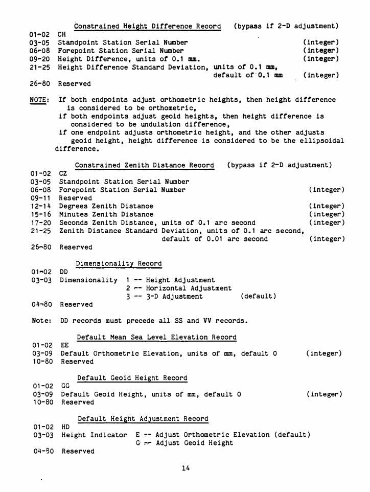
Constrained Height Difference Record 01�02 CH 03-05 StandpOint Stat ion Serial Number
Forepoint Station Serial Number Height Difference , units of 0.1 mm . Hei ght Difference Standard Deviation,
06 ... 08 09-20 21-25
(bypass if 2-D adj ustment)
(integer) (integer)
26-80 Reserved
units of 0.1 mm, default of-O. l mm
(integer)
(integer)
NOTE: If both endpoints adjust orthometric heights , then height difference is consi dered to be orthometric ,
i f both endpOints adj ust geoid height s , then height difference is consi dered to be undulation difference ,
if one endpOint adj usts orthometric height , and the other adj usts geoid hei ght , height difference i s considered to be the elli psoidal
di fference .
Constrained Zenith Distance Record (bypass if 2-D adj ustment ) CZ Standpoint Stat ion Serial Number Forepoint Stat ion Serial Number R es erved Degrees Zenith Distance Minutes Zeni th Distance
01-02 03-05 06-08 09-11 12-14 15-16 1 1-20 2 1 -25
Seconds Zenith Distance , units of 0.1 arc second Zeni th Distance St andard Deviation , uni t s of 0.1 arc second ,
default of 0.01 arc second 26 ... 80 R eserved
Dimens ionali ty Record 0 1 ""02 DD 03-03 D imensionalit y
04 .. 80 R eserved
1 Height Adj ustment 2 ,..- Hor izontal Adj ustment 3 3-D Adj ustment ( default )
Not e : DD records must precede all SS and VV records .
Deraul t Mean Sea Level Elevat ion Record 0 1 -02 EE 03-09 Default Orthometr i c Elevat ion , uni ts of Mm, default 0 10-80 Reserved
Default Geoid Height Record 0 1 -02 GG 03-09 Default Geoi d Height , units of Mm, default 0 1 0-80 R eserved
Default Height Adjustment Record 0 1 -02 HD
( integer )
( integer ) ( integer ) ( integer )
( integer )
( integer )
( integer )
03-03 Height Indi cator E �- Adjust Orthometr i c Elevat ion ( default ) G� ... Adj ust Geoi d Height
04-130 Reserved
14

0 1 "'02 HC Control POint Height Adjustment Record
03-03 Height Indicator E -- Adj ust Orthometric Elevat ions ( default ) G -- Adj ust Geoid Heights
0�-06 Station Serial Number 01-80 Reserved
Iterat ion Record II 0 1 .-02
03-04 05.-08 09- 1 1 1 2- 1 1 1 8- 1 8
Maximum number of iterations , default 5 Maximum allowable misclosure , units of sigma , default 300 Minimum printed misclosure , un its of sigma , default 30 Coordinate convergence tolerance, units of mm, default 3 Display stat isti cs when solution slowly converges
( integer ) ( integer ) ( integer ) ( integer )
y � ... Display stat istics N -- Do not display statistics ( default )
1 9,.,80 Reserved
Adjustment Mode Record 01 "02 MM 03�03 Mode indi cator 0 -- Simulation , bypass cc04�1 2 of this record
1 �- Compute quasi�normal res iduals ( default ) 2 Compute q . n . res iduals and inverse 3 . . Compute normal res iduals and inverse
04-04 Post-adj ustment indicator N Do NOT scale s i gmas by a posteriori var iance factors ( default )
Y Scale weights 05�05 Update *80* Control Point Records with adjusted pos itions
N -- Do NOT update *80* records ( default ) Y -- Update *80* records
06- 1 2 New Blue Book filename ( alphanumer i c ; default for the new Blue Book filename -- ' NEWEB ' )
0 1 -02 03-03
04,,04
05-05 06...,08
09"'09 1 0�1 0 1 1 -1 1 1 2- 1 2 1 3- 1 3 1 4- 1 4 1 5..- 1 5 1 6- 1 6
Pr int OutEut Record PP Echo Blue Book F ile. 0 Echo
1 Echo 2 Echo
Echo G'-Format Fi le 0 Echo 1 Echo 2 Echo
Display Constraints Cri ter i a for Resi dual Output ( XX . x ) 0 . 0 Display All Res iduals ( default ) 1 . 0 Di splay Only Normal ized Residuals 99. 9 Display No Residuals ( 1 00 , 000 , 000 Display D irect ion Res i duals Display Angle Residuals Display Zeni th Distance Resi duals Display Distance Res i duals Display Asto�Azimu�h Resi duals Display GPS Res iduals Display Constrained Res i duals Display Res i duals Grouped Around
15
all ( default ) observat ions only large misclosures only all ( defaul t ) observations only large misclosures only
(nonblank to defeat option )
Greater or Equal to 1 . 0 sigma )
( nonblank to defeat opt ion ) " " n " n n n " n " " " " " n " " " " " " " " "

Intersection Stations 17-17 Display Position Shirts 18-18 Display Googe Numbers 19-19 Display the Observational Summary 20,..20 Display the Adj usted Positions 21�0 Reserved
Accuracy Computation Record 01",02 QQ 03-10 Reserved 11-13 Station Serial Number , required 14-:50 Reserved 51-53 Station Serial Number , required 54�80 Reserved
"
"
"
tI
tI
CPS Rot at i on Parameter Record
01-02 RR 03-04 05.-08 09:-10 11"'12 13-14 15..,16 17.-17 18-21 22-23 24-25 26-27 28-29 30�30 31-80
Res erved Start Year , default 1801 Start Month, default 01 Start Day , default 01 Start Hour, default 00 Start Minute , default 00 Time Code , Start Time , default Z End Year , default 2100 End Month, default 12 End Day , default 31' End Hour , default 23 End Minute , default 59 Time Code , End Time, default Z Reserved
•
"
"
n
"
Auxi l iary Parameter Indi cator and Constraint Record 01-02 03-04
SS Observation Type 25
40 52 54
Start Year� default 1801 Start Month, default. 01 Start Day, default 01 Start Hour , default 00 Start Minute , default 00
CPS ( scale ) Vertical Angle ( refraction ) Reduced Distance ( scale ) Reduced Long Line ( scale)
Time Code , Start T ime , default Z End Year , default 2100 End Month , default 12 End Day , default 31 End Hour , default 23 End Mi nute, default 59 Time Code , End Time , default Z
" tI
fI
•
•
"
"
"
. "
"
(integer )
(integer)
(integer ) (integer) (integer ) (integer) (integer )
(integer ) (integer) (integer ) (int eger ) (integer )
(integer ) (integer ) ( integer!) (int eger ) (integer )
(integer ) ( integer ) (integer ) (integer ) (integer )
05,..08 09,..10 11-12 13-111 15-16 17..,17 18..,21 22-23 24,..25 26�27 28"'29 30"'30 31:-35 Scale value or refraction , uni ts of 0.00000001 (0.01 ppm ) , ( integer )
36-40 default 0
'
Std . Dev. of Scale , units of 0.01 ppm , default 100
16
( integer ) ,

41..,80 Reserved
01-02 03-04
Variance Factor Indicator & Constraint Record vv Observation Type 20 � - Horizontal Direction
25 .-- GPS 30 40 52 54 60
Start Yea r , default 1 80 1 Start Month, default 0 1 Start Day , default 01 Start Hour , default 00 Start Minute , default 00
Horizontal Angle Vertical Angle Reduced Dis tance Reduced Long Line Laplace Azimuth
Time Code , Star t Time , default Z End Year , default 2 1 00 End Month , default 1 2 End Day , default 3 1 End Hour , default 2 3 End Minute , default 59 Time Code , End Time , default Z
( integer ) ( integer ) ( integer ) ( integer ) ( integer )
( integer ) ( integer ) ( integer ) ( integer ) ( integer )
05-08 09.-1 0 1 1 - 1 2 1 3'-1 4 1 5-1 6 1 7- 1 7 1 8-.21 22-23 24r25 26-27 28-29 30- 30 3 1 -35 Ini tial Estimate of Variance Factor , units of 0 . 0 1 , default 1 00
36�36 Absolute Constraint Y N
37.-80 Reserved
( integer ) Impose Constraint Do NOT Constrain ( default )
Records may appear in any order in an AFILE , with two exceptions . If 88 records exist , they must precede any occurrence of DD , SS , RR , or VV records . If DD records exist , they must precede any occurrepce of SS , RR , or VV records . There are no restr i ctions on the order of SS , RR , or VV records , except that they must come after BB and DD records .
The Ell ipso id Parameter Record ( AA ) is used to select an ell i psoid. If this record is not present , then the adj ustment wi ll refer to the Geodet ic Reference System of 1980 ( GRS 80 ) ell ipsoi d. This is the reference ell i psoi d used by the NAD 83 datum. If the user needs to compute an adj ustment using the NAD 27 datum , the parameters for the Clarke 1866 ell ipsoid are:
semimaj or axis a 6378206 . 400 square of first eccentr icity • 0 . 006768657997291
The 8ypass Record (B8) is used to bypass different types of observat ions . I f the record is not present , then the adj ustment will not bypass types o f obs ervat ions .
Notable except ion : ,If a two-dimens ional or a one�dimens ional adj ustment is selected ( see the DD record ) , then certain types of observat ions are automatically bypasse d , e ven if a 8ypass Record ( 88 ) is not included .
17

The Constrained Coordinate Record (CC) is used to constrain (or fLx) any combination of a station ' s geodeti c latitude , geodetic longitude and height . I f this record is not present , then no coordinates will b e constrained . This vill result in a s ingular adj ustment and premature termination. Therefore , at �east one CC record should exist in any AFILE . (In fact , an AFILE may well contain only one record : a CC record) .
The station serial number and the coordinate values do not possess default values ; these fields must be completed to receive that const raint . I f a·two� dimensional adj ustment is computed (see DO record) , then the height field is ignored . I f a oner.dimensional adj ustment is computed, then the geodetic lati tude and geodeti c longitude fields are .ignored. In addition , the user can constrain only latitudes , longitudes , or heights in any combination (subj ect to the constraints proposed by the d imens ionali ty of the adj ustment) . For example , one can constrain the lati tude, but not the longitude or height , at a station by completing only the geodetiC lat i t ude fi eld.
P lease not e , when a field (latitude , longi tude or height) is to be constrained , that particular fi eld must not be blank. For exampl e , if the user needed to constrain a landmark to a hei ght of zero , then the height field must contain zeros and not be blank .
The standard deviations of a constraint are optional , and possess default values of 0 .1 mm. A standard deviation is i gnored unl ess its associated constraint value is present .
The CC records are formatted such that the fields of the constraint values correspond to the f i elds of the Blue Book *80* records . This enables the user to retrieve coordinates from a data base or compute coordinates from other adj ustments , quickly edit these coordinate records , and then use the new records as constraints.
The height constraint is consi dered to be an orthometric hei ght constraint if the or thometric height of the st at ion is being adj usted. (See HC record . ) The height constraint is considered to be a geo i d height constraint i f the geoid hei ght of the station is being adj uste d . Therefore , if a one�dimens ional or a three-dimens ional adj ustment is being computed, be sure to check that the values in the he ight constraint fields actually represent the type of hei ght you wish constrained.
The Constrained Astronomic Az imuth Record ( CA ) is used to constrain a mark-to� mar k azimuth relat ion . I f this record is not present , then this constraint is not included . This record is ignored on a one�dimensional adj ustment . ( See DD recor d . ) The stat ion ser i al numbers are not opti onal . I f the value of the azimuth constraint is not prov ide d , the adj ustment will use the ini t i al values of the stat ions ( from the *80* records ) to compute the constraint value . If the user wi shes to provi de a constant value , do not apply the Laplace correction . The standard deviation of the constraint is opt ional .
The Constrained D i s tance Record ( CD ) is used to constrain a mark�to�mark distance relat ion . I f this record is not present , then this constraint is not included . The st ation seriai numbers are not optional . I f the value of the distance constraint is not provided , the adj ustment wi ll use the initial values
18

of the stations ( from the *80* records) to compute the constraint value. The standard deviat ion of the constraint is opt1onal .
The Constrained Zenith D1stance Record ( CZ) is used to constrain a mark-tomark zenith distance relat ion . If this rec�rd is not present then this constraint is not included . This record is ignored on a tw��dimens ional adjustment . ( See DD record . ) The stat ion ser ial numbers are not optional . If the value of the zeni th distance constraint is not provided, the adjustment will use the initial values of the stations ( from the *80* and *84* records) to compute the constraint value . The standard deviation of the constraint is opt i onal . I f the user wi shes to provi de a particular value for a zenith distance constraint , then that value sho ul d not be contaminated by any poss ible refract ion error .
The Constrained Height D i fference Recor d ( CH) constrains a hei ght difference relat ion . If this record is not present , then this constraint is not included. This record is i gnored on a two�dimens ional adj ustment . ( See DD record . ) The constraint is consi dered to be an orthomet r i c hei ght difference i f both endpoints adjust their orthometric heights . ( See HC recor d . ) The constraint is cons i dered to be a geoid he i ght difference·i f both endpoints adj ust their geoid height s . The constraint is considered to be an ellipsoidal hei ght d i fference if one endpoint adjusts its orthometric he ight whi le the other endpoint adjusts its geo i d he i ght . The station ser ial numbers are not optional. If the value of the height d ifference constraint is not provi de d , the adjustment will use init ial values of the stations ( from the *80* and *84* records ) to compute the constraint value . The standard deviation of the constraint is optional .
The D imens ionality Record (DD ) is used to select the dimens ionali ty of the adjustment . If this record is not included , a three�dimens ional adjustment is computed . If a two�dimens ional adjustment is selected, then zeni th distances and zenith distance constraints are automati cally bypassed , and the he i ght coord inate for each stat ion is automat ically held f ixed at its initial value . If a one-dimensional adjustment is selected , then the direct ions , angles , astronomic azimuths , and azimuth constraints are automati cally bypassed, and the geOdetic lat i tude and geodetic longitude for each stat ion are held f i xed at the ir init ial value . The user can. always request addi tional types of observations to be bypassed by use of a SS record . A DD record should not be placed ahead of a SS record. SS , RR , and VV records should not be placed ahead of a DD record . The Default·Mean Sea Level Record (EE ) is used to spec ify a default value for the orthometr ic he i ght of each stat ion . If this record is not present , zero is used for the default value of the orthometr i c he i ght . In pract ice , the user will always have an or thometr ic height present in the *80* records , so thes e values will overri de the default orthometri c hei ght .
The De fault Geo i d He ight Record ( GG ) is us ed to speci fy a default value for the geoid hei ght of each stat ion . If this record is not pres ent , zero is used for the default value of the geoid he ight . Values of the geoi d hei ght in the *84* records will overr i de the default geo i d he i ght . If the user does not have an *84* record for some stat ions , then this record can eas i ly be used to indicate an approx imate geoid he ight for the project .
The Default Height Adjustment Record ( HD ) is used to select whe ther the orthometr i c he i ghts or the geo id he ights of the stat ions are adjusted. If this record is not present , the orthometric hei ghts will be adjusted . This record is
19

ignored i f a two�dimensional adj ustment is being performed . The Control Point Height Adj ustment Record ( HC ) is used to select whether the orthometric height or the geoid height of a particular stat ion is adj usted. I f this record is not present , the adj ustment will use the default command selected in the HD record. The HC record is i gnored if a two-dimensional adjustment is being performed .
I n a typical si tuation the user wants t o adj ust orthometri c hei ghts , but certain stat ions may be bench marks . A decision may be made to include HC records for the bench marks , us ing the " G" indicator to refine estimates of the geo id he ight in the region . These improved geoid he ights could then be included in a later adj ustment us ing the " GG" or *84* records .
The Iterat ion Record ( II ) i s used t o control the iterat ion and misclosure display of the adj ustment . If this record is not present , the default actions specifi ed in table 2 . 2 are taken. I f the adj ustment cycles past the maximum number of i terat ions , or if a misclosure exceeds the spec ified limi t , a terminat ion flag is raised. However , the user can still request that statistics be displayed when the terminat ion condition has occurred. The misclosure limits are defined i n units of standard deviation. Not e , for example , if a particular distance has a standard deviat ion of 1 . 5 cm and the computed minus the observed distance is 25 s i gma , the actual misclosure for that particular distance is 31 . 5 cm. ( Misclosure equals sigma un i ts multiplied by the standard deviation . )
If the user does not have good preliminary coordinates , the s ize of the maximum allowed misclosure and of the minimum printed misclosure may be increased . This will prevent a premature terminat ion due t o bad starting coordinates . The large misclosures wi ll decrease as the coordinates are improved . I f blunders are present in the data, they could cause the adjustment to di verge , and thereby exceed the maximum number of iterat ions . Misclosures would " di sappear " around the poor preliminary coordinates and " appear" around the blunders . Even i f the iteration limit were exceeded , the user would probably wish to see the statistics displayed to help locate those problems .
The Adj ustment Mode Record ( MM ) is used to select the mode of operation . I f this record is not present , the. default act.ions spec ified in table 2 . 2 are taken . The modes are arranged in order of increasing computational time . Mode one displays resi duals scaled relat i ve to the standard deviat ion of the . observat ion ( quas i�normalized resi duals ) . These quasi�normal i zed r es iduals somet imes give an erroneous indicat ion of which observation contains a blunder . Mode two also displays quasi�normalized res iduals and computes a part ial , sparse inverse to allow the display of coordinate standard deviations and accuracy computat ions . Mode t hree computes r es i duals scaled relati ve to the standard dev iat ion of the residual ( normali zed residual ) . Normali zed residuals can be used much more successfully in locating outl iers. I f any VV records are used , then mode three is automat ically invoked .
Mode zero is a special simulation mode. In this mode , observations and their standard dev iations are used to compute network statistics using linear error propagation . The observat ion values themselves are ignored, and need not be coded . This mode is provided to evaluate network deS i gns before field operat ions commence .
The postadj ustment indicator can be used to scale all of the error propagat ion statistics by the a posteriori var i ance of uni t wei ght . This indicator should
2 0

not be used unless the observational data are of one type , and there i s poor knowledge of the observation wei ghts . It is not recommended that this indi cator be used unless one is sure that, blunders have been eliminated , that no systemati c errors are presen t , that one does not have good initial estimates of the observat ion standard deviations , and that a chi-square stat ist i cal test indicates the a posterior i estimate is s i gni f icantly different than 1 . 0 . This option is automati cally disabled when comput i ng a simulation ( mode - 0 ) .
I t i s also possible to request that a new copy of the input Blue Book file be create d where the *80* and *84 * records are updated with new adj usted values . This f i le will be named "HEWBB" unless a different file name is s pecified. The creat ion of a new Blue Book i s disabled when computing a simulation ( mode � 0 ) .
The Pr int Output Record ( PP ) is used to control the amount of pr inted output . I f this record is not present , then the maximum amount of print ing is generated. The spec i f ications in table 2 . 2 detail exactly what output is controlled by this recor d . Typically , an output sect ion is generated unless a nonblank character appears i n an appropriate column . The cr i teria for res i dual output are based on the magni tude of the normal i zed ( or quasi�normalized ) res idual . The default value , 0 , displays all res i duals . A number such as 300 displays only those normali zed residuals greater than 30 . 0 . If a s imulat ion is bei ng computed (mode - a i n the MM record) , then coordinate shifts will not be computed or displayed .
The Accuracy Computation Record ( QQ ) is used to compute relat i ve accuracy stat i s t i cs between selected stations . If this record is not present , then these computat ions will not be performed . The stat ion ser ial numbers ar e not optional . These computat ions can help to locate weaknesses in the network and to determine the, provis ional accuracy classi fi cat ion of the survey .
The GPS Rotat ion Parameter Record ( RR ) is used to allocate extra parameters ( unknowns ) to the adjustment . If this record is not present , then no extra rotat ion parameters wi ll be allocated. An RR record should not be placed ahead of a BB or DO record.
Thes e parameters are defined according to time span . The default t ime span ranges from the years 1 80 1 through 21 00 . The time codes are identi cal to those found in the Blue Book � While it is possible to wholly contain one or mor e time spans wi thin a longer time span ( i . e . , "nes ted" time spans ) , a user will probably seldom need to allocate parameters i n this way.
The Auxiliary Parameter Indi cator and Constraint Record ( SS ) is used to compensate for systemat i c errors , due to refract ion or scale error by aSS igning extra parameters ( unknowns ) to the adj ustment . If this record is not present , then no extra parameters will be included. An SS record should not be placed ahead of a BB or DO record.
The parameters are defined according to observation type and time span . The observat ion type is not opt ional . A refraction parameter is created for zenith distances , and a scale parameter is created for other observation t ypes . The default t ime span ranges from the years 1 80 1 through 2 1 00 . The t i me codes are ident i cal to those found iri the Blue Book . Time spans are not allowed to overlap for a gi ven observation type . It is poss ible to wholly contain one or more shorter time spans within a longer time span ( that is , "nested" time
2 1
spans ) . However , the user would probably seldom have a need to assign parameters in this fashion.
With prior knowledge of the scale error or refracti on , perhaps due to an earlier adj ustment or a base l ine cal ibration, the user can apply this informat ion as a constraint . The constraint is created if the parameter value and/or standard deviation is coded. No constraint is created if both fields are left blank .
Indiscr iminate ass i gnment of auxiliary parameters will weaken a survey proj ect , perhaps to the point of givi ng a s i ngular solution . Survey redundancy and mult i ple connections to the control network are encouraged if auxiliary parameters need to be part of the adj ustment solution .
The Var i ance Factor Indi cator and Constraint Record ( VV ) is used to readj ust observat ion we ights along wi th the coordinates . If this record is not present , then no wei ght r escaling wi ll take place . The VV record should not be placed ahead of a BB or DO record. The var iance factor is a term whi ch multiplies the square of the standard deviation of an observation. Therefor e , i f the standard deviation is 3 cm and the var iance factor is 4 , then the rescaled standard deviat ion woul d become 6 cm . Use of this record will automat i cally invoke a mode 3 adj ustment ( see MM record) and require s i gnificant computat ion time .
The var i ance factors are defined according to observation type and time span . The observat ion type is not optional . The default t ime s pan ranges from the years 1 80 1 through 2 1 00 . The time codes are ident i cal to those found in the Blue Book . Time spans are not allowed to overlap for a given observation type . It is possi ble to wholly contain one or more shorter time spans wi thin a longer time span ( that i s , " nested" time spans) . However , var iance factors would seldom need to be ass i gned in this fashion .
If the user has pr ior knowledge of a variance factor � perhaps due to an earlier adj ustment , then this knowledge can be applied as a constraint . This is done by coding the absolute constraint field, using i t as a mechanism to rescale standard de viat ions without edi t ing every observat ion record in the Blue Book . Do not attempt to est imate var iance factors wi thout redundant measurements of the appropriate observat ion type . For example , it is impossi ble to compute the var iance factor for the s ingle distance measurement in a s pur traverse .
To compute a var iance factor rat io ( FGCC 1 98 4 ) for a par t i cular observation type , f irst obtain a variance factor estimate from knowledge of standard deviation or from a minimally constrained , mode 3 adj ustment of the surve y. Then combine the survey data with the surrounding network data, and compute a much larger , minimally constrained adj ustment . However , in this combined adj ustment , the us er would es t imate var iance factors for the survey obs ervat ion types . The output would display the fi nal est imates of the survey variances , the init ial es timates , and the var i ance factor rat i o . When this ratio exceeds 1 . 5 , systemat i c error between the s urve y and the network is usually the cause . Both the s ur vey data and the network data should be i nspected . The es timate of the variance factor rat io becomes more reliable as the number of survey connect ions to the network is increased.
2 2

Error Messages
Error messages generated by ADJUST fall into two categories . anticipated error messages and programmer error messages . Anticipated error message are those which describe the various error condi t ions that occur due to incorrect formats . s ingular solutions . insufficient memory . etc . These messages and the ir diagnoses are descr i bed in table 2 . 3 and 2 . 4 . res pect i vely .
Programmer error messages locate errors in the program logic and operat ion. These messages should never be encountered and i nvari ably result in an immediate terminat ion . If any programmer error message occurs in table 2 . 5 . please contact the National Geodetic Survey . NOS . NOAA.
Table 2 . 3 . --Anticipated error messages
1 . No AFILE��All defaults active 2� *********Note : Semimaj or axis - nnn 3 . *********Note : Eccentr icity - nnn 4 . ***Warning : Negat ive VTPV 5 . Slowly converging solut ion 6. Slowly converging var iance factor solut ion 7 . nnn ***Lar ge misclosure 8 . nnn Double prec ision words is too small for nnn parameters 9 . nnn D . P . wor ds less than nnn needed for rank-nnn insuffic ient
storage--fatal ! 1 0 . Insuffic ient storage for constrained astro . azimuth 1 1 . Insuffic ient storage for constra ined zen i th distances 1 2 . Insufficient storage for constrained distances 1 3 . Insuffici ent storage for constrained height distances 1 4 ; Insuffici'ent storage for accuracy computat ions 1 5 . Insuffic ient storage for hor . d irections 1 6 . Insufficient storage for hor � angles 1 7 . I nsuffic ient storage for zeni th distances 1 8 . Insuffic i ent storage for reduced d istances 1 9 . Insuffic ient storage for Laplace az imuths 20 . Insuffi c i ent memory for GPS vectors nnn 2 1 . *** Illegal adj ustment file format type-- ( AFILE recor d ) 22 . The BB record must precede the SS and VV records 23 . Illegal dimens ion�- ( AFILE record ) 2 4 . Auxiliary parameter table over flowed--record ignored 25 . Duplicates the nnn�th aux . parameter record 26 . Illegal observat ional type 27 . Var iance factor table overflowed�-record ignored 28 . Duplicates the nnn-th var iance factor record 29 . No *80* control point records encountered�-fatal 30 � No Blue Book found--fatal error 3 1 . nnn is i llegal SSN�- fatal 32 . nnn dupl icates the nnn-th entry--fatal 33 . Over 700 landmarks 34 . No *80 * records :for-- ( Blue Book record ) 3 5 . ( Blue Book record ) nnn i s illegal SSN-- fatal 36 . ( Blue Book record ) nnn dupli cates the nnn entry--fatal 37 . Illegal time code�- ( time code )
2 3
38 . I llegal azimuth degrees a nnn 3 9 . ( G�Format record) NVEC-nnn exceeds MAXVEC-nnn 40 � Too many C records , bad G-file structure , ( G-Format record ) 4 1 . Bad �file str ucture-� ( card merge ) 42 . I llegal correlat ion--nnn , nnn 4 3 . Bad correlation index nnn 44 . *** warning--diagonal correlat i on nnn , nnn 4 5 . Correlation matrix s ingular i ty-�nnn 46 . Terminated due to misclosures ( C-O ) /SD exceeding 4 7 . nnn FDF-nnn **** is s ingular ******** 48 � Terminated due to var i ance factor singular i t ies 49 . The following nnn unknowns fall below tolerance of nnn 50 � nnn ( stat ion name ) North/ south shift googe number i s nnn 5 1 . nnn ( station name ) East/west shift Googe number i s nnn 52 � nnn ( stat ion name ) Up/ down shift Googe number i s nnn 5 3 . nnn the nnn � t h aux . parm. Googe number is nnn 54 . nnn the nnn -th rot . parm� Googe number is nnn for l i s t U nnn , at nnn
( stat ion name ) 5 5 . The adj ustment is si ngular ! ! 5 6 . ***** fatal-�undetermined ( U ) stat ions ***** 57 . U pdated control point records in fi le-- ( file name ) 58 . No old Blue Book found. 59 . Not able to open new Blue Book f ile 60; Fatal error flag due to previous errors 6 1 . The number of vectors in a group - nnn has exceeded the maximum
62 . 63 . 64 . 65 . 6 6 . 67 .
allocated - nnn The BB record must precede the DD , SS , RR , and VV records GPS rotat ion parameter table overflowed�-record i gnored Dupli cate the nnn-th GPS rotat ion parameter record The x component of the nnn�th aux . GPS rot . par am o Googe The y component of the nnn- th aux. GPS rot . param� Googe The z component of the nnn- th aux . GPS rot . par am o Googe
Table 2 . �--Diagnosis of data messages
1 . Check filename and j o b control used to execute ADJUST 2. Confirm this is the des i red semimaj or axis 3 . Confi rm this is the des ired eccentr icity squared
number number number
is is is
� . Check for large mis closures or blunders in the obser vat ional data
nnn nnn nnn
5 . Chec k for large misclos ures . May need to incr ease maximum number of iterat ions .
6 . Variance factor solut ions are not always rap i dly conver gent . Incr eas e maximum number of i terat ions .
7 . Check record book , pos s i bly rej ect the obser vat ion by placing an "R" in column 6 of the Blue Book or an "R" in column 58 on the C record in the GPS data Transfer G- Format .
8 . I ncr ease the internal program st orage of ADJUST . ( See "Mod ifying the Memory Allocat ion" in sec . 4 . )
9 . Same as N o . 8 10. Same as No. 8 11 . Same as No . 8 12 . Same as No . 8
24
Same as Same as Same as Same as Same as Same as
2 5

i dent i f i cation . 50 . May need to constrain the lat i tude using the CC record in the AFILE 51 . May need to constrain the longi tude using the CC record in the AFILE 52 � May need to constrain the hei ght using the CC record in AFILE 53 . Check the network geometry . Increased redundancy is necessary when
allocating auxiliary parameters . 54 . Loose tr iangle. Check all the list of direct ions of the
standpo int stat ion for the connect ivity of each list . May need to combine two l ists .
55 . Companion message to No . 4 9 56 . Ver i fy network geometry . Check dimensionali ty or possibly constrain
stat ions us i ng the CC record in AFILE . 57 . Verif y file 58 . Same as No . 30 59 . Check i f newly selected Blue Book filename confli cts wi th existing
f ilename 6 0 . Refer to previous error messages 6 1 . Increase the parameter NVEC i n all o f the parameter st atements . 62 . Place BB record ahead of DO , SS , RR , and VV records 63 . Ei ther request fewer GPS rotat ion parameters or increase internal arrays .
See "Mod ifying the Memory Allocat ion" in sec . 4� ) 64 . Check dupl icat ion . GPS rot at ion parameter time spans may not overlap . 65 . Same as 5 3 . 66 . Same as 53 . 67 . Same as 53 .
Table 2 . 5�-Yrogrammer messages
1 . ( AFILE recor d ) *** Record not in parameter table 2 . Il legal IVFannn for Nannn for OBSH 3 . Illegal IVFannn for Nannn in BIGL 4. Fatal error in Googe computat ion in FINAL nnn 5 . State error in invers ion of VFCVRG 6 . State error in VFCVRG 7. Profile error in VFCVRG 8 . State error in prop of VFGPS 9 . Profi le error in prop of VFGPS
1 0 . Error in GETGIC--nnn 1 1 . GPS index overflow in PUTICM 1 2 . Illegal values in FORMICannn 1 3 . Illegal k ind in FORMCannn 1 4 . ********* Illegal IVFannn for Nannn in FIXVF 1 5 . Premature file end in FORMG�-NVECannn 1 6 . Illegal k ind in COMPOBannn 1 7 . Il legal values in IUNSTA nnn 1 8 . Ille gal values in IUNAUX nnn 1 9 . Illegal values in IUNROT : IZannn NZannn 20 . Illegal value in INVIUN nnn 21 . Illegal values in IUNSHf
'nnn
22 . Profile error in NORMAL 23 . Accum error in NORMAL
2 6
24 . Fatal Googe error in NORMAL nnn 25 . HOG state error in NORMAL 26 . Premature file end in NORMAL--NVEC-nnn 27 . I llegal type code nnn 28 . Illegal icode in SINGUL nnn 29 . Programmer error in CONVRG 39 . Illegal parameter code in CONVRG--nnn 3 1 . Basement window error�-nnn 32 . Fatal error in Googe computat ion in FINAL nnn 33 . State error in FINAL 34 . SSN table error in OBSSUM--nnn 3 5 . Illegal IVFannn for N-nnn in ROBS 36 . System not inverted in ROBS 37 . All convariance elements not within profile�-ROBS 38 . I llegal k ind in ROBS�-nnn 39 . Premature file end in RGPS-�NVEC-nnn 40 . State error in first prop of GPSSDV 4 1 . Profile error in f irst prop of GPSSDV 42 . Illegal IVF-nnn for N-nnn in GPSSDV 43 . State error in PROPCV of GPSSDV 44 . Profile error in PROPCV of GPSSDV 4 5 . State error in second prop of GPSSDV 46 . Profile error in second prop of GPSSDV 47 . Get sigma error in ADJAUX��nnn 48 . I llegal IVF-nnn for N-nnn in RESID2 49 . System not inverted in RESID2 50 . All convariance elements not within profi le--nnn 5 1 . I llegal kind in RESID2 .... ,..nnn 52 . Premature file end in RESID2--NVEC-nnn 5 3 . Premature file end in DUMRD �,.. NVEC-nnn 54 . SSN table error in ADJPOS--nnn 5 5 . Get s igma error in ADJ POS�nnn 56 . I llegal ISN in UP80--nnn 57 . Illegal ISN in UP84--nnn 58 � State error in RELACC 59 . Prof ile error in RELACC 60 . ****illegal ISN nnn for NSTA-nnn in PUTALA 6 1 . ****i llegal ISN nnn for NSTA-nnn 1n PUTALO 6 2 . ****illegal ISN nnn for NSTA-nnn i n PUTGLA 63 . ****illegal ISN nnn for NSTA-nnn 1n PUTGLO 64 . ****illegal ISN nnn for NSTA-nnn in PUTECX 65 . ****illegal ISN nnn for NSTA-nnn in PUTECY 66 . ****illegal ISN nnn for NSTAannn in PUTECZ 67 . ****illegal ISN nnn for NSTA-nnn in PUTMSL 68 � ****i llegal ISN nnn for NSTAannn in PUTGH 69 . *** *illegal IAUX nnn for NAUX-nnn 1n PUTAUX 7 0 . ****illegal I Z nnn for NZ-nnn in PUTROT 7 1 . ****illegal ISN nnn for NSTA-nnn in GET ALA 7 2 . ****illegal ISN nnn for NSTA-nnn 1 n GETALO 73 . ****illegal ISN nnn for NSTA-nnn in GETGLA 74 . ****illegal ISN nnn for NSTA-nnn in GETGLO 75 . ****i llegal ISN nn� ' for NSTA-nnn in GETECX 76 . ****i llegal ISN nnn for NSTA-nnn in GETECY 77 . ****illegal ISN nnn for NSTA-nnn in GETECZ
2 7

78 . ****illegal ISN nnn for NSTAannn in GETMSL 79 . ****illegal ISN nnn for NSTA-nnn in GETGH 80 . " ****illegal IAUX nnn for NAUXannn in GETAUX 8 1 . ****illegal IZ nnn for NZannn in GETROT 82 . Get s i gma error in ADJGRT 83 . I llegal IGRT - nnn for NGRT - nnn in PUTGRT 84 . Illegal IGRT a nnn for NGRT a nnn in GETGRT
3 . MATHEMATICAL MODELS
This section covers var ious coordinate systems and the mathemat i cal models ( observat ion equations ) used by program ADJUST . These mathematical models include the least squares adj ustment models , observat ion models , correlations , and var iance models .
Coordinate Systems
The default ell ipsoi d used by ADJUST is the Geodetic Reference Sys tem , GRS 1 980. However , in pr inci ple , an ell i pso i d is not needed for performing an adj ustment in three dimens ions . ADJUST is a computer program used for adj ust ing po ints ( stat ions ) in space using a local geodetic hori zon system . ( See fig. 3 . 1 . ) ADJUST uti l izes a local astronomi c hor i zon system ( LAHS ) to set up the observat ion equat ions . The observat ion equat ion coefficients are then transformed into those appropr iate for local geodetic hor izon systems ( LGHS ) . The di fferential shifts of coordinates are in li near units ( meters ) in a geode tic hor i zon sys tem centered on the points in ques t ion ; thus , ther e are as many loca} coordinate syst ems as there are stat ions .
When the surveyor observes hor izontal or vert i cal theodoli te observat ions in the field , the geodetic observat ion is not meas�ed . Rather , the astronomi cal observat ion is measured ( e . g . , an astronomic az imuth is observed, not a geodet i c azimuth ) . Therefore , an important relat ionshi p between coordinate systems i s the one between the LAHS and the LGHS . ( See f i g . 3 . 2 . ) Instruments are ali gned tangent to the plumb l ine ( or the grav ity vector ) , not to the ellipsoid normal . ( See f i gs . 3 . 1 and 3 . 2 . ) Theory requires that the d irect ion of grav i ty be known at all stat ions from wh ich theodol i te observat ions are measured . Because this is seldom achieved , some approximat e values must be used for astronomi c coordinates . Thes e preliminary astronomic lat i tudes and longi tudes are computed us i ng the prel iminary geodetic lati tudes and longi tudes and the deflect ions of the ver t i cal . If the deflections are not present , ADJUST will set the deflect ions equal to zero ; henc e , the prelim inary astronomic coord inates are set res pecti vely to the most recent geodetic values . As a step in process ing , ADJUST trans forms the observation equat ions from the local astronomi c hor izon system to the local geodetiC hori zon system us ing rotation matr i ces ( Steeves 1 98 4 ; V incenty 1 979 ) .
The LGHS and the LAHS do have simi larit ies . Both reference systems are three�dimens ional Cart es ian systems wi th their or igins at the point ( station ) i n quest ion . However , their axes are di fferent whenever the deflect ion of the ver ti cal i s known to be nonzero . For the LGHS and the LAHS , we will refer to the ir axes as ( x , y , z ) and ( u , v , w ) , respecti vely. The LGHS has a z-axis that is co incident wi th t he ell ipso id normal at the stat ion and is pos i t i ve upwards .
28

The LGHS x-axis points to the geodetic north and the y-axis points to the geode t i c east . The w-axi s of the LAHS i s coincident wi th the gravity vector at
x
z • I
_ , "',..oido/ ""'0/ /.----- of P
,
k.,.-+---;---+--- Y
Fi gure 3 . 1 . --Local geodetic hori zon system ( Steeves 1 98 4 )
z
, \ .
I
xj t r----"",
A ,
x
ton9, nt to p 'umb . in, / ___ ---- ot P
� ____ Itotion morller
\ ---- . o ltronomlC I I
\ I , I
"
Y
..,ridian p'on,
F i gure 3 . 2 . -- Local astronomic hor izon system ( Steeves 1 984 )
2 9

the station and is posi tive upwards . The u-axis points to the astronomic north while the v�axis points to the astronomic east.
The relationship between the LGHS and LAHS is defined by :
t t ( x , y , z) "" R ( u , v , w ) ( 3 . 1 )
where R is a rotat i on matr i x which performs the transformation from the LAHS to the LGHS . V incent y ( 1 980 : eq. 6 ) der ives that
sin� · ( A- A ) ( � � )
R "" T
RG
RA
.. -sin� ' ( A- A ) cOS� ' ( A- A )
- ( � -� ) - coM ' ( A- A )
where
-sin</> COSA -s in</> s inA cos</>
R "" G
-5inA COSA 0
cos</> COSA cos</> s inA 5in� -
and
- 5 i n� cosA -s in� s inA cos�
R .. A
-sinA cos A 0
cos� cosA coM s inA sin�
where ( <1> , A ) are the geod e t i c lat i tude and long i t ude and ( � , A ) are the ast ronomi c lat i tude and long i tude .
E quat ion ( 3 . 1 ) can also be wr i t ten as
where
x .. u + m ' v + l · w y "" v - m · u + n · w z .. w - l · u - n · v
m .. s �n� • ( A - A ) n .. cos� • ( A - A ) 1 .. ill - Ij>
3 0
( 3 . 2 )
C 3 . 4)

The Least Squares Problem
The least squares problem is minimize
Q ( X ) 3 V ( X )t �l V ( X ) ( 3 . 6 )
b
where V ( X ) is a resi dual funct ion ( Dennis and Schnabel 1983 ) . Consider the method of observation equat ions ( Mi khail 1976 or Uot i l a 1967 )
L 3 F ( X ) ( 3 . 7 ) a a
where L is a vector of computed observation values of length n , X is a vector a of model parameters of length u , and F is a vector of funct ions that is a theoret i cal model which descr ibes the observat ions in terms of the parameter s .
I n this method
where Lb
is the vector of actual observations .
Assume model F ( X ) is not strongly nonlinear and the problem is a small a
( 3 . 8 )
res i dual one . These simpli fying assumptions allow se lection of the Gauss-Newton method of solut ion.
The des ign matr i x , A , is defined as
aF I A .. ax X .. X a a 0
where A i s a matrix of di fferential changes in the observation model with respect to the parameters , X , evaluated at a part icular set of parameter
a values , Xo ' A vector of observation misclosures is
L .. L - L b a
where Lb and L
a are descr ibed above .
( 3 . 9 )
( 3 . 1 0 )
Associated wi th the observation vector Lb
is a symmetr ic variance-covar iance
matri x EL
' wh ich contains informat ion on observat ion precis ion and correlation . b
The observat ion equation may be wr i tten as
AX .. L + V ( 3 . 1 1 )
3 1

where V is a vector of resi dual errors and X is a vector of corrections to the parameter vector X
a. The least squares estimate of X is
Thi s is a solution of the normal equations
NX .. U
where the matrix of normal equat ion coeffic ients is
and the right hand vector is
One techni que for solut ion is to compute a Choles ky decomposi t ion of the normal matr i x , N ,
NX .. Rt RX .. U .
( 3 . 1 2 )
( 3 . 1 3 )
( 3 . 14 )
( 3 . 1 5 )
( 3 . 1 6 )
The est imate of X provides a new set of values for our parameters by replacing
X + X + X • a a
( 3 . 1 7 )
If the observat ion model F ( X ) is nonli near ( that is , A is not constant for any a
set of X ) , then the ent ire process starting with eq . ( 3 . 6 ) , must be iterated a
unt i l the vector X reaches a stat ionary pOint . a
Est imates of parameter prec is ion and correlat ions are given by the adj usted parameter var i ance-covar i ance matr i x , L This matr i x is computed by
x a
( 3 . 1 8 )
Of course , this matr i x can always be scaled by an est imated var iance of uni t we ight , i f such an es t imate i s felt val i d . The user may also compute the
32

precis i on of any other quantity which can be deri ved from the parameters . Suppose one wishes to compute a vector of quant i t i es , S ,
S .. S ( X ) a
from the adj usted parameter s , X . A geometry matri x , G , i s def ined as a
• X o
( 3 . 1 9 )
( 3 . 20 )
where G is a matrix of different ial changes in the functions , S , with respect to the parameter s , X , evaluated at a part icular set of parameter values , X • a 0
By the pr inciple of l inear error propagation,
or
where r is the var iance-covar iance matr i x of the computed quant i t i es . s
( 3 . 2 1 )
( 3 . 22 )
This last equat ion is useful since i ts terms are quanti ti es der i vable from the parameters . I t could be used , for example , to compute r
v or L
L •
a
Another useful quantity is the correlation coeffi c i ent p , where
( 3 . 2 3 )
and 0 . . is the value in the i-th row and j -th column of the adj usted parameter lJ var i ance-covar i ance matr i x , r
xa
Thes e correlat ions can be thought of as a
normalized covar ianc e , s ince
-1 � p � 1 • ( 3 . 2 4 )
Correlations between para�eters that approach + 1 indicate ill�condi t ioning of the system .
Several sparse matr ix pac kages have been introduced by various author s , George and Liu ( 1 98 1 ) , Dillinger ( 1 98 1 ) and Mi lbert ( 1 984 ) . Each of these packages
3 3
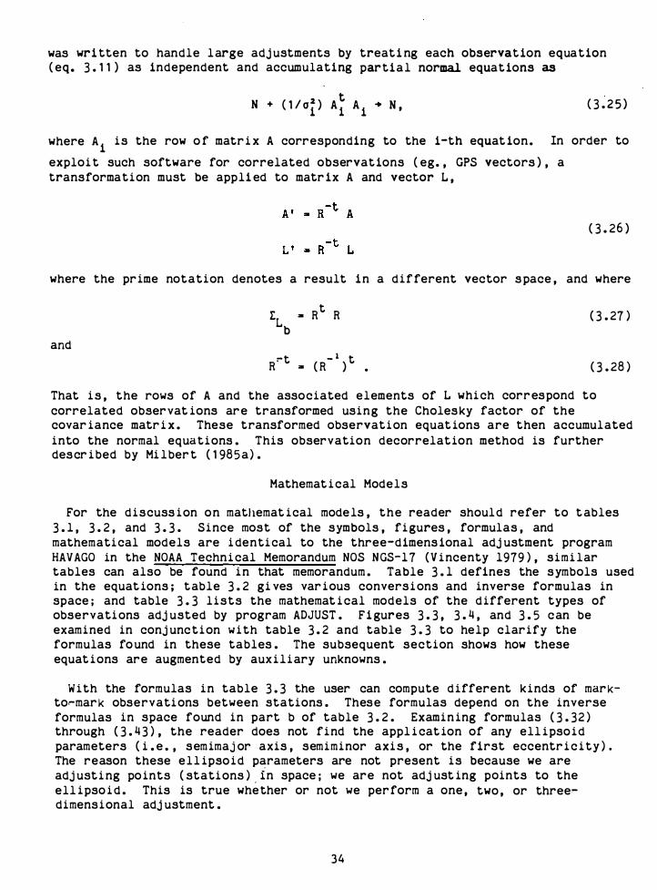
was wri tten to handle large adj ustments by treati ng each observation equation ( eq. 3 . 1 1 ) as independent and accumulating partial normal equat ions as
N + ( 1 / °1 ) A� Ai
+ N , ( 3 . 2 5 )
where Ai
is the row o f matr i x A corresponding to the i-th equat ion. In order to
exploi t such software for correlated observat ions ( eg. , GPS vectors ) , a transformation must be appli ed to matr ix A and vector L ,
( 3 . 26 )
where the prime notation denotes a result in a different vector s pace , and where
LL 3 Rt
R b
( 3 . 27 )
and
R�t _ 1
)t 3 ( R . ( 3 . 28 )
That i s , the rows of A and the associated elements of L whi ch correspond to correlated observat ions are transformed using the Cholesky factor of the covar iance matr i x . These transformed observation equat ions are then accumulated into the normal equations . This observation decorrelation method is further descr ibed by Mi lber t ( 1 98 5 a ) .
Mathemat i cal Models
For the discuss ion on mathemat ical models , the reader should refer to t ables 3 . 1 , 3 . 2 , and 3 . 3 . Since most of the symbols , fi gures , formulas , and mathemati cal models are i denti cal to the three-dimens ional adj ustment program HAVAGO in the NOAA Techni cal Memorandum NOS NGS-1 7 (V incenty 1979 ) , simi lar tables can also be found in that memorandum . Table 3 . 1 defines the symbols used in the equat ions ; table 3 . 2 gi ves var ious convers i ons and inverse formulas in space ; and table 3 . 3 lists the mathemat i cal models of the different types of observations adj usted by program ADJUST . Fi gures 3 . 3 , 3 . 4 , and 3 . 5 can be examined in conj unc tion w i th table 3 . 2 and table 3 . 3 to help clarify the formulas fo und in these tables . The subsequent section shows how these equat ions are augmented by aux iliary unknowns .
With the formulas in table 3 . 3 the user can compute different kinds of mar kto�mar k observations between stations . These formulas depend on the inverse formulas in space found in part b of table 3 . 2 . Examin ing formulas ( 3 . 32 ) through ( 3 . 4 3 ) , the reader does not find the appl i cat ion of any ell ipsoid parameters ( i . e . , semimaj or axis , semiminor axi s , or the first eccentr i c i ty ) . The reason these ell ipso id parameters are not present is because we are adj ust i ng po ints ( stations ) , in space ; we are not adj ust ing pOints to the ell ipso i d . This is true whether or not we perform a one , two , or three� dimens ional adj ustment .
34

Table 3 . 1 . --Symbols and definitions
a Semimajor axis of t he ellipsoi d b Semiminor axis of the elli psoid e First eccentricity of t he ellipsoid e ' Second eccentr icity M Radius of curvature in the mer idian N Radi us of curvature in the prime vertical � geodetic latitude , pos i tive north A Geodet ic longitude , pos i tive east h Geodetic height ( he i ght above ellipsoid ) � Astronomic lati tude A Astronomic longi tude H Height above the geo i d A Astronomic azimuth , clockwi ze from the north V Vertical angle, pos i ti ve upward from the astronomic hori zon S Spat ial distance XYZ Ri ght-handed , three-dimens ional ( Earth-centered fi xed ) Cartesian
coordinate system whose Z-axis is defined by the Conventional International Origin ( CIO ) , and the XZ plane is parallel to the Mean Greenwich Zero Meri d ian.
xyz Right-handed , three-dimensional ( local geodeti c hori zon system ) Cartes i an coordinate system whose z�axis is coinc idental with the elli psoid normal at station in question ; x-axis points to geodeti c north, and y-:ax is points to geodetic east.
uvw Right-handed , three-dimens ional ( local astronomic hori zon system ) Cartes ian coordinate system whose w�axis is co incident wi th the gravity vector at station in question ; u�axis points to astronomic north and the vO- axis points to astronomic east .
F'orcpO i n l
p 'I' p
S tandpo in t S tandpoint R
S tandpoint
F'o repo i n t
'I'
Fi gure 3 . 3 . --Top view. Fi gure 3 . 5 . ·--Perspecti ve view .
( excerpted from Vincenty 1 979 )
35

Table 3 . 2 . --General equat ions
a. Conversion of ( � , A , h ) to ( X , Y, Z )
X 3 (N+h) cos� COSA
Y 3 (N+h) cos� sinA
Z - [N ( l-e�) + h] s in�
b . Components in the local astronomic hor i zon system . (See figs . 3 . 3 . 3 . 4 , and 3 . 5 . )
6Z 3 Z 2 - Z l
P l 3 -sin� 1 ( 6X COSA l + 6Y sinA l ) + 6Z COS� l
Q l 3 -6X s i nA l + 6Y cosA l
R l 3 ( P 1 2 + Q 12 )
1 /2
T l 3 cos� 1 ( 6X cOSA l + 6Y sinA l ) + 6Z s in� l
Similarly , we have at pOint #2
Table 3 . 3 . --Mathemat ical models ( mark-to�mar k )
a . For GPS vectors :
3 6
( 3 . 29 )
( 3 . 30 )
( 3 . 3 1 )
( 3 . 32 )
( 3 . 3 3 )
( 3 . 3 4 )
( 3 . 35 )
( 3 . 3 6 )
( 3 . 3 9 )
( 3 . 4 0 )
( 3 . 4 1 )
( 3 . 4 2 )
( 3 . 4 3 )

flY ,. Y 2 - Y 1 < 3 . 4 4 )
b. For astronomic azimuths :
< 3 . 4 5 )
c. For astronomic d irections :
< 3 . 4 6 )
where n i s an ori entation unknown for each independently measured set of directions.
d. For astronomic zenith distances :
e . For mark�to-mark distances :
f . For astronomic hor i zontal angles :
Table 3 . 4 . --0bservat ion equat ions ( mark-to-mar k )
a . GPS vectors :
Vt:.x ,. a 1
V ,. !:J.y
b 1
V ,. c 1 !:J.z
b . Az imuths :
dX 1
dX 1
dX 1
c . Directions :
+ a2
+ b2
+ c 2
d . Zeni th distances :
dY l + a3
dY l + b 3
dY l + c 3
dZ 1 + a .. dX 2 + as
dZ 1 + b .. dX 2 + b s
dZ 1 + c .. dX 2 + C s
3 7
dY2 + a, dZ 2 + K
t:.x
dY2 +
dY2 +
b , dZ 2 + K !:J.y
c , dz 2 + K t:.z
+ d, dw 2 + K a
0 . 4 1 )
< 3 . 4 8 )
< 3 . 4 9 )
< 3 . 50 )
< 3 . 5 1 )
< 3 . 52 )
< 3 . 53 )
VZD
'"' f l dU l + f 2 dV l + f , dW l + f_ dU2 + f5 dV 2 + fa dW2 + KZD ( 3 . 55 )
e . Distances :
Vs '"' g l dX l + g2 dY l + g 3 dZ l + g_ dX 2 + g5 dY2 + ga dZ 2 + Ks ( 3 . 56 )
f . Hor izontal angles :
Vh
.. h l dU l + h2 dV l + h 3 dU2 + h_ dV 2 + h5 du , + ha dv , + Kh ( 3 . 57 )
Table 3 . 5 . --Coeffi c i ents of observat ion equat ions
a l '"' R G( l , l ) l .. s i n� l COSA l
a 2 '"' RG
( 2 , 1 ) 1 '"' s i nA l
a 3 .. RG (
3 , 1 ) 1 .. -COSq, l COS A l ( 3 . 58 )
a .. .. RG
( l , 1 ) 2 .. -s i n � 2 COS A 2
a s .. RG
( 2 , 1 ) 2 .. - s i n A 2
a , .. RG
( 3 , 1 ) 2 '"' COS � 2 COS A 2
b l R G( 1 , 2 ) 1 .. s i nq, l s i n A l
b 2 .. RG
( 2 , 2 ) 1 .. - COSA 1
b 3 '"' R G ( 3 , 2 ) 1 .. - COSq, l s in A l
b .. .. RG
( l , 2 ) 2 .. - s i nc h s i nA 2 < 3 . 59 )
b s .. RG( 2 , 2 ) 2 .. COS A 2
b , .. RG( 3 , 2 ) 2 .. COS q, 2 s i nA 2
c 1 .. R G( 1 , 3 ) 1 .. - COSq, l
C 2 '"' R G( 2 , 3 ) 1 .. 0
3 8
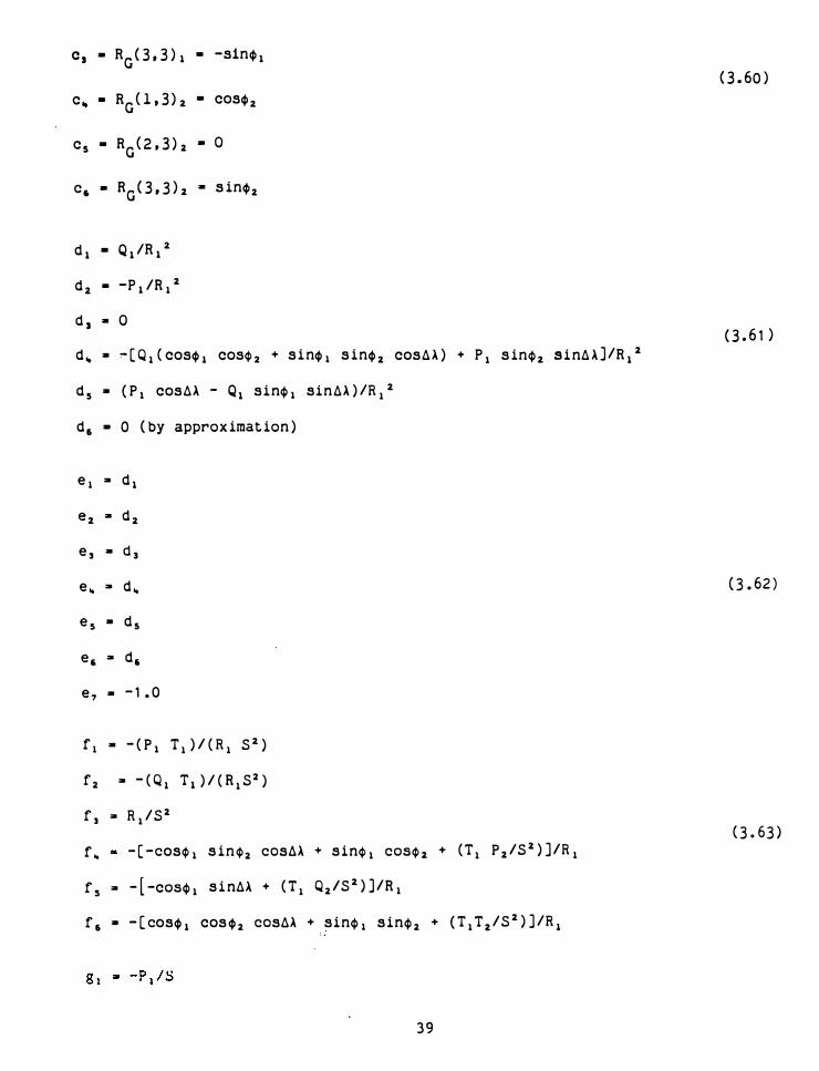
C , .. RG < 3 , 3 ) 1
Cit • RG( 1 , 3 ) 2
C s • RG
( 2 , 3 ) 2
c. .. RG < 3 , 3 ) 2
d 1 • Q 1 /R 1 2
d 2 .. -P 1 /R 1 2
d , .. 0
- -S1n� 1
• COS� 2
.. 0
.. S in�2
d .. .. � [ Q l ( COS� l COs� Z + S i n� 1 S in� 2 COS6 A ) + P I S in$ 2 s i n6 A ] /R 1 2
d S .. ( P I COS6A - Q 1 Sin$ 1 sin6A ) /R 1 2
d . .. 0 ( by approx imat ion )
e 1 .. d 1
e 2 .. d 2
e , .. d 3
e .. .. d ..
e s .. d s
e • .. d,
e 7 .. - 1 . 0
f l .. - ( P I T 1 ) / ( R 1 S 2 )
f2 .. - ( Q l T 1 ) / ( R 1 S Z )
f 3 .. R 1 /S 2
f .. - [ -COS� 1 s in�2 COS6A + s in� 1 C05� 2 + ( T 1 P 2 /S 2 ) ] /R 1
f 5 .. - [ -C05$ 1 s i n6A + ( T 1 Q2 /S 2 ) ] /R 1
f . .. - [ COS� l COS � 2 COS6A + Sin$ 1 S in$ 2 + ( T 1 T z /S 2 ) ] /R l
3 9
< 3 . 60 )
< 3 . 6 1 )
C 3 . 62 )
< 3 . 63 )

g2 a �Q 1 /S
g , a -T 1 /S ( 3 . 64 )
g � a -P 2 / S
g s 2 -Q 2/ S
g 6 a -T2 /S
h l a d 1 ( r i ght ) - d 1 ( le f t )
h 2 a d2 ( r i ght ) - d 2 ( left )
h , 2 - d � ( left )
h � a - d s ( left )
h s a d � ( r i ght )
h 6 a d s ( r i ght )
Looking at eqs . ( 3 . 53 ) , ( 3 . 54 ) , ( 3 . 55 ) , and ( 3 . 57 ) , the reader not i ces that the d i ffer ent ial shi fts are in a local geode t i c hor i zon ( coor d i nate sys t em ) . R espec t i vely , K
AX' K
AY and K
AZ are the d i f ferences between the computed and
observed GPS vectors ( AX , Ay and �z ) . The observat ion equat ions for azimuths , d irect i ons , zeni th d is t ances , and hor i zontal angles are formed us ing local astronom i c hor i zon d i fferent ial s h i ft s . A f t er the coeff i c ients for these observat ion equa t i ons ( eqs . 3 . 5 3 , 3 . 54 , 3 . 55 , and 3 . 57 ) are compute d , ADJUST uses a rot at i on mat r i x ( eq . 3 . 2 ) to · transform the observat i on equat ions from an LAHS to the LGHS . S i nce the observat ion equat ion for mark- to-mar k d i st anc es ( eq . 3 . 5 6 ) cont ains the d ifferent i al shifts i n an LGHS , no trans forma t i on i s required . Aga i n , t h e l a s t term ( K
a, K
d, K
Z D' K
s' and K
h) o n t hese observa t i on
eqs . ( 3 . 5 3 through 3 . 57 ) are the d i f ferences between the computed and the observed observa t i ons .
There is a s l i ght dependence of the astronom i c az imuths and d ir e c t i ons on the ver t i cal d i fferent ial shi ft of the forepo int ( target ) . However , follow i ng V i ncenty ( 1 97 9 ) we take the coeff i c ients o f the observa t i on equat ions , d 6 and e 6 to be zero . Note that the observat i on models , ( 3 . 5 3 ) and ( 3 . 54 ) , ar e s t i l l computed r i gorous l y . I n keeping wi th t h i s approx imation , the ver t i cal d i fferent ial shifts for the hor i zont a l ang l e observat ion eq . ( 3 . 57 ) are suppressed .
All of the obser vat ion equations in table 3 . 4 are set for a thr ee-dimens i onal adj ustment . But ADJUST also has the capab i l i ty for one� and two- d i me ns i onal adj ustments . S i nce a one-d imens ional adj ustment w i l l mod ify onl y the . ver t i cal component , only two coeff i c i ents are needed for the appropr i a t e observat i on equat ions . Thes e two coef f i c i�nts ar e the ver t i cal components o f the s t andpoint and the forepo in t . They are equal to the th ird and s i x th coeff i c ients o f the ir
4 0

respect ive coeffi c i ents found in table 3 . 5 . Likewis e , when performing a twodimens ional adj ustment , only the hor i zontal components will reflect shi fts and the vert i cal components are held fixed. Hence , for a two-dimensional adj ustment , only four coeffi c i ents are required . These four are for the hor i zontal components of the standpoint and the forepoint . Again , these four will equal the first , second , fourth, and f i fth coeff icients of their respective coeff i c i ents found in table 3 . 5 . The unneeded coeffi c i ents are never formed nor accumulated into the normal equat ions .
Or ient at ion Unknowns and Aux i l i ary P arameters
As ment ioned previously, an or i entat ion unknown ( 0 ) exists for each independ� ently measured set of directions . These or ientation unknowns are pr esent only if ADJUST is performing a two- or three-dimensional adj ustment containing direct ion observations .
In addition to ori entat ion unknowns for hori zontal directions , ADJUST can comput e var ious types of auxi l i ary parameters ( AP ) . These AP ' s can cons ist of GPS rotati on unknowns , refract ion unknowns for zenith distances , or scale unknowns for spatial distances and GPS vectors . Table 3 . 6 shows the modi f ied observat ion models . Table 3 . 1 contains these additional coeffi c i ents whi ch would be attached to the respective observat ion equation ( table 3 . 4 ) when needed .
a .
b .
Table 3 . 6 . --Modified observat ion models
GPS vectors ( scale parameter � k )
llX � llX - k ' llX
llY � llX - k e llY
llZ � llX - k - llZ
GPS vectors ( rotat ion parameters � ( wx' wy '
( by Rapp 1 9 83 : pp . 6 1 -6 4 , 1 38 )
- - -llX
llY
llZ
� RG
t R RG o w 0
llX
llY
llZ
wz) )
where RG
is ( 3 . 3 ) evaluated at a mean point ( � o , A o ) , o
and where
4 1
< 3 . 6 6 )
< 3 . 6 7 )

Thus ,
where
1 1 -
£ 2 -
R -w
6X • I:J.X +
-I:J.Y • I:J.Y -
I:J.Z • I:J.Z -
1 1 1 1 1 2
-w X
I:J.Y + 1 2 I:J.Z
I:J.X + 1 , I:J.Z
I:J.X - 1 , I:J.Y
COS � o (jJ + sin <P o (jJ x Z
s i n CP o sin ). 0 (jJx - cos ). 0 (jJ - cos CP o Y
c . Zen i th d is tances ( refract ion parameter - k ) ( by Rapp 1 983 : p . 1 � 9 , eq. 56 )
d . Spat ial distances ( scale parameter • n )
s . S - k ' S
sin ). 0
Table 3 . 7 . --Aux i l i ary parameter coefficients
a. For GPS vectors ( scal e ) :
b . For GPS vectors ( rotat ions about ( x , y , z ) axes at ( � o , A o »
4 2
(jJ z
( 3 . 6 8 )
( 3 . 69 )
( 3 . 7 0 )
( 3 . 7 1 )
( 3 . 7 2 )
( 3 . 7 3 )
( 3 . 7 L, )
< 3 . 7 5 )

c , - -cos A O ( X2
c . For zeni th distances ( refraction ) :
11 a f l + k • P i IR l 12 a f2 + k · Q 1 IR l
f , a f , ( 3 . 7 6 )
1� a f� - k · P i IR l 15 a f 5 - k · Q 1 IR l
1, a f,
17 a -R 1 d . For spat ial distances ( scale ) :
( 3 . 77 )
Variance Models
In the publication Standards and Specificat ions for Geodet i c Control Networks ( FGCC 1 984 ) , a four-step process is descr ibed wh ich leads to the accuracy class i ficat ion for a proj ect submi tted to the NGS ( Mi lbert 1 985b ) . The first step details examining all aspects pertaining to the incoming surve ys ( e . g . measurements , field records , sketches , etc . ) for compl iance wi th the measurement system spec i f i cations . Next , a least squares adj ustment performed on the survey a i ds in the detection of blunders and verif ies correct we i ghting of each observat ion . The third step is also part of the least squares adj ustment . This step computes the length relat i ve accuracies by error propagat ion in order to ' determine the prov is ional accuracy. The final step is comput ing a var iance factor by the Iterated Almost Unbiased Estimator ( lAUE ) method (Lucas 1 985 ) . Var iance factors serve to detect some systemat ic errors .
4 3

Once the vari ance factor is computed , a vari ance factor rat io test is performed . The var iance factor ratio is the var iance factor o f the new survey combined with the network data , divided by the var i ance factor of the survey alone . This test helps detect systematic error s , poss ibly in the control network , possibly in the incoming survey , or possibly in bot h. This final step helps determine that a survey i s accurate and not merely precise ( Mi lbert 1 98 3 ) . However , the use of var iance factors to detect systemat ic error is not foolproo f . For example , a global scale error is not detectable in a minimally constrained survey adj ustment ( FGCC 1984 ) . A survey wh ich was connected to the network at only one or no exis ting control pOints would not be able to detect systematic error between the survey and the networ k .
The vari ance factor for the new survey i s computed b y the lAUE method . In this me thod , the observations are grouped into k groups , to each of which is assoc iated a vari ance factor , f . 1
where �L is a symmetric var i ance-covar iance matrix which contains informat ion
b on observation precis ion and correlat ion. From the above equat ion we can now est imate k different local var iance factors,
f l � 1 0 0 0
0 f 2 � 2 ° 0 � '" L
b 0 0 f
k �ko
The initial es timate of the k-th vari ance factor in the above model can be wr i t ten as
f .. k
where Mi 1 bert ( 1985 ) computes Q ( the central redundancy matr i x ) as
Q .. I .• W .. I - R -t A N _ l A
t R - 1
Table 3 . 8 shows the equations for the var ious error analys is quantit ies wh ich can be computed in ADJUST . The software allows the opt ion of comput ing ei ther a pr iori or a posteriori stat i s t i cs . The a poster iori var i ances are scaled by the sample var iance of unit we i ght�
44

o
where n is number of observat ions u is number of unknowns .
n - u
If more detai l is required , Mi lbert ( 1 985a) and Baarda ( 1 96 8 ) may be consulted.
Table 3 . 8 . --General error analysis equations
a. Quas i-normalized residuals ( v ' )
V I • vi oL b
where v is the res idual and 0L standard deviation of b
the measured observat ion.
b. Standardized ( normal ized) res iduals (v)
v . v/ o v
where a is the st andard de viation of the res i dual . v
c . Redundancy number ( q )
where 0L is the stanaard deviation of the computed observat ion . a
d . Marginally Detectable Errors ( MDE )
MDE • ( ). 2 I ) 1/2 °L q b
where ). was pres elected as 9 .
4 5

4 . PROGRAM IMPLEMENTATION
The f irst phase of process ing ins i de ADJUST is to determine the options required in the run . This is done by process ing the adj ustment file in subrout ine AFI L . This process ing also determines the number o f auxi li ary parameters to be allocated in memor y.
Memory Maps
In program ADJUST , a large array , A , is assi gned . ADJUST then manages th is space to fit the parti cular adj ustment problem.
Figur e 4 . 1 d isplays the memory map for ADJUST . The user may wish to refer to SUBROUTINE ALOCAT while reading the map . Once the number of stat ions , NSTA , and the number of parameters , NUNK , have been determined , the storage can be allocated. Each of the regions on the main map are further subdivi ded according to figures 4 . 2 through 4 . 5 .
Fi gure 4 . 2 shows the arrangement in the Data Storage Block. The function GETPRM is us ed to compute an index into the auxiliary parameter sub�block . Function GETZ computes an index into the direction or ientat ion parameter sub�block . The funct ion GETSSN can be us ed to compute an index ' into the remainder of the Data Storage Block.
Fi gure 4 . 3 gi ves the arrangement of the Googe numbers ( Schwarz 1 918 : 29- 32 ) . This arrangement is also the mapping of the order of the parameters . As with the Data Storage block , funct i ons GETPRM, GETZ and GETSSN can be used to compute indi ces . Since this arrangement is also the parameter order , function INVIUN can be used to determine parameter types when gi ven an index to a Googe numbers .
Fi gure 4 . 4 displays the memory map for the posi t ion shifts . The shifts are in the respec t i ve local geodetic hor izon sys tems ( x , y, z ) . This region can be indexed by con verting a Blue Book Station Ser ial Number ( SSN ) into an internal stat ion number ( ISN ) us ing GETSSN . The ISN is then used as input for IUNSHF .
Fi gure 4 . 5 displays the map for the work area used for decorrelation of the GPS vector s . This area is allocated for a maximum of f i ve correlated GPS vectors ( MAXVEC � 5 in subrout ine ALOCAT ) . The work area is then re-par t i t ioned for each vector set ( NVEC � 1 or NVEC � 2 ) . The upper triangular covar iance matr ix is stored in columns 1 through Nl . The Cholesky factor is computed in place . The var iances are stored in column 1 , rows 2 through N R . Column N2 is a scratchpad col umn for decorrelat ion by subrout ine COMRHS . The routi nes GETRHS and PUTRHS load and unload this scratchpad column , respect i vely .
The or iginal and the decorrelated coeffic ients o� the observation equat ions are stored in columns N2+ l through N3 . Misclosures are stored in column N4 , and the measured observations are stored in column N5.
When mode 3 processing is selected SUBROUTINE GPSSDV uses a sli ghtly different map of the work area . The normali zed res i duals are stored in column N2 . The standard deviation of the resi duals are stored in column N4 . Redundancy numbers are stored in column N 3 . destroying the observat ion equation coeffic ients .
4 6
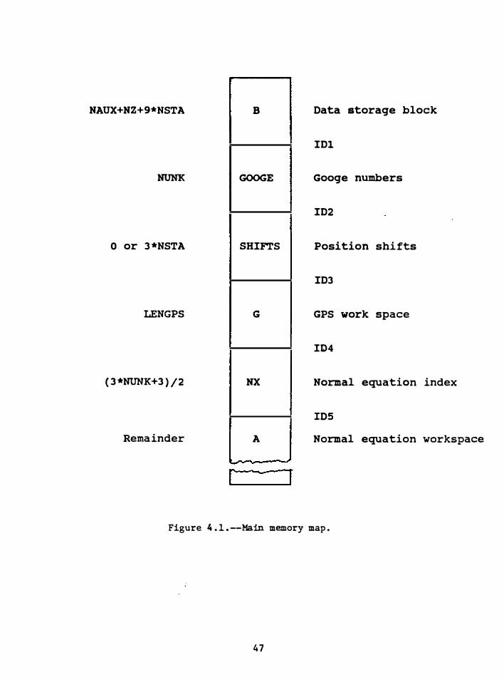
NAUX+NZ+9*NSTA B Data storage block
101
HUNK GOOGE Googe numbers
102
o or 3 *NSTA SHIFTS Position shi fts
103
LENGPS G GPS work space
ID4
( 3 *NUNK+3 ) / 2 NX Normal equation index
IDS
Rema inder A Normal equation workspace
- -
Figure 4 . 1 . --Main memory map .
4 7
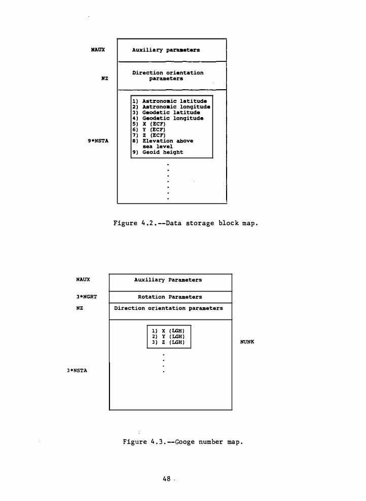
KAUX Auxiliary parameters
Direction orientation NZ parameters
1) Astronomic latitude 2 ) Astronomic lonqitude 3 ) Geodetic latitude 4 ) Geodetic lonqitude 5 ) X ( ECF) 6 ) Y (ECF) 7 ) z (ECF)
9*NSTA 8 ) Elevation above sea level
9 ) Geoid heiqht
· · · · · · ·
Figure 4 . 2 . --Data storage bloc k map .
NAUX Auxiliary Parameters
3 *NGRT Rotation Parameters
NZ Direction orientation parameters
1 ) X ( IJ;H ) 2 ) Y ( IJ;H ) 3 ) Z ( IJ;H ) HUNK
· · ·
3 *NSTA
Figure 4 . 3 . --Googe number map .
4 8

NR
( 3 *NVEC)
1) X (LGH) 2) Y (LGH) 3) Z (LGH)
Figure 4 . 4 . --Po s it ion shift memory map .
NR 1 LENG - (NVEe + 1 ) * 3
W Observation equation
o coefficients
R
K
N1 N2
F igure 4 . S . --GPS wo r k area memory map .
4 9
N3
1 1
M 0 I B S S C E L R 0 V S A U T R I E 0 S N
s
N4 NS

In mode 0 , which completes a simulat ion , marginally detectable errors (MOE) are stored in column N2 .
The remainder of main memory is allocated to an index array, NX , and the normal equat ion array, A . Detai ls on these arrays may be found in Mi lbert ( 1984 ) .
Data Structures
The most heavily used special data str ucture in ADJUST is an array used to convert Blue Book Stat ion Ser ial Numbers ( SSN ) into internal st ation numbers ( I SN and JSN ) . This array is held in the common block named SSNTBL . The routi nes NEWSSN , GETSSN , PUTSSN , and LOCSSN insulate the user from direct ( and potent ially erroneous ) manipulat ion of the index array.
Aux i l iary parameters and vari ance factors are keyed by a time span and an observat ion type code . Separate named COMMON blocks hold the work arrays . As with the SSN table , thes e routi nes convert the keying informat ion into an index . The direct ion or ientations are k eyed us ing a SSN and a l ist number . Other than the fact that a different key is used , the ori entation uti l i ty rout i nes funct ion in the same fashion as the other s .
Mod ifying the Memory Allocation
If i t is necessary to increase or decrease the s ize of main memory , this is easily done in the main program . Mod ify the parameter named LENA . Th is will automat ically cause LNWORK and LAWORK to be set to appropri ate values .
If it is necessary to decrease the s i ze of the SSN indexing down from 999 , modify rout ines NEWSSN , GETSSN , PUTSSN , and LOCSSN . Note that the use of large legal SSN ' s wi ll result in error messages if this modi f i cat ion is performed . Addi tional al located space can b e reduced by modi fying the stat ion indexing down from 999 in routines OBSSUM , NEWI , and CONTR .
If more than five sets of rotation parameters are needed , modi fy the COMMON block named /GRTTB2/ in routines PUTRTG and GETRTG.
If more than 30 auxi l iary parameters are needed , modify rout ines NEWPRN , GETPRM , and PUTPRM .
If more than 30 variance factors are needed , modify routines NEWIUF GETIU F , PUTIUF , and FIXIUF .
If more than 700 intersection stat ions are observed , modify routi nes NEWFOT and RESID2 .
If more than 3000 or ientat ion unknowns ( lists ) are needed , modify routines NEWZ , GETZ , PUTZ , LOCZ , and INVZ .
If more than five GPS vectors ( C records ) are observed per sess ion (B recor d ) , modify all instances of the parameter named NVEC . Use of a global sear ch and replace ed it funct ion is recommended .
5 0
Implementat ion Restri ctions
Since Fortran 77 requires predeclaration of the s i ze of an array, certai n lengths have been encoded into ADJUST . Note that the following numbers may vary based upon the par t icular computer version of ADJUST .
Main memory ( LNWORK ) : Maximum SSN : Rotat ion parameters Auxi liary parameters : Var iance factor s : D irection or i entation unknowns : ,Landmarks : GPS vectors per session :
200 , 000 integer words 999 5 30 30 3000 li sts 700 5
These restrictions wi ll gi ve rise to the ant i c i pated error messages numbers : 8 through 20 , 24 , 27 , 33 , 39 , and 63 in table 2 . 3 . One may be able to c ircumvent these problems by increas i ng the storage allocation in ADJUST .
Machine Dependent Features
It is assumed that the INTEGER type declarat ion provides at least 32 bits to store an integer , and that the DOUBLE PRECISION declarat ion prov ides at least 60 bits to store a floati ng point number to suff icient accuracy . It is also assumed that the number of bits in two INTEGER words is equivalent to the b i ts in one DOUBLE PRECISION word.
Operat ing System Dependent Features
An " implici t " assumption of ADJUST is that a lar ge amount of memory is ava ilable to store the A ( ) array . If a virtual memory operat ing system is used , no problems should aris e . Some operating systems requi re explicit declaration of the virtual arrays . Table 4 . 1 indi cates the var ious " alias" names of the A ( ) array .
Table 4 . 1 . --Arrays stored in A ( ) array
A NX B GOOGE SHIFTS G
If a virtual memor y operat ing system is not avai lable , the user may wish to decrease the s i ze of the A ( ) matr i x , as di scussed ear l i er . I f large systems need to be solved without virtual memory , ADJUST will need to be modified to use an "out of core" normal equat ion sol ver such as LASSO ( or BIBB ) ( D illinger 1982Y�
Language Extens ions
No language extens ions from the Amer ican Nat ional Standards I nsti tute (ANSI ) standard ANSI X 3 . 9-l978 ( FORTRAN 77 ) have been used .
51

Special Compi ler Options
No spec i al compi ler options have been used in the development of ADJUST .
ACKNOWLEDGMENTS
The authors wish to ac knowledge the programming and debugging support of Al ice Drew . They are greatly indebted to Eleanor Andree , whose ass istance went far beyond the call of duty .
REFERENCES
Baarda , W . , 1 9 6 8 : A tes t i ng procedure for use i n geodetic networks . Publi cat ions on Geodesy , New Series , 2 ( 5 ) , Netherlands Geodet i c Commiss ion ,
Delft .
Dennis , J . E . and Schnabel , Robert B . , 1 983 : Numer ical Methods for Unconstra ined Opt i m i zation and Nonl inear Equat ions . Prentice-Hal l , Inc . , Englewood C l i ffs , NJ , 324 pp .
Dilli nger , Will iam H . , . 1 98 1 : Subrout ine package for large , sparse , least squares problems . NOAA Techn ical Memorandum NOS NGS-29 . Nat ional Geodetic Information Center , NOAA , Rockv i l le , MD 1 8 pp .
EI-Hak im , S . F . , 1 98 1 : A pract i cal study of gross-error detection in bundle adj ustment . The Canadian Surveyor , 35 ( 4 ) , 37 3-38 6 .
Federal Geodetic Control Comm i t tee , 1 9 8 4 : Standards and Spec i f icat ions for Geodetic Control Networks . - Nat ional Geodet i c Informat ion Center , NOAA , Rockv i l le , MD , 29 pp .
r George , Alan and Liu , Joseph W . , 1 9 8 1 : Computer Solution of Large Sparse
Pos i t i ve Defini t i ve Systems . Prenti ce-Hall , Inc . , Englewood C l iffs , NJ , 324 pp.
Lucas , James R . , 1 985 : A var iance component es t imat ion method for sparse matrix appl i c at ions . NOAA Techn i cal Report NOS 1 1 1 NGS 33 . Nat ional Geode t i c Informat ion Center , NOAA , Rockv i lle , MD , 1 2 pp .
Mikha i l , Edward M. , 1 9 76 : Observat ion and Least Squares . IEP Dun-Donnelley , New Yor k , NY , 285-288 .
Milbert . Dennis G . , 1 985a : A note on observat ion decorrelat ion , var iances of res i duals , and redundancy number s . Bulletin Geodes ique , 59 , 7 1 - 80 .
Mi lbert , Dennis G . , 1 9 85b : Appli cat ion of the var i ance factor test to a Gl obal Pos i t ion ing System surve y . Proceed ings of the 4 5 th Annual Mee t i ng of the Amer ican Congress on Survey ing and Mapping , Washington , DC , March 1 0- 1 5 , 1 9 85 .
Mi lbert , Dennis G . , 1 98 4 : Heart of Gold : Rout ines for large , sparse least squares computat ions . NOAA Techn ical Memorandum NOS NGS�39 . Nat ional Geodet i c Informat ion Center , NOAA , Rockville , MD , 28 pp .
Milbert , Dennis G . , 1 9 8 3 : A spec i f i cat ion is not a class i f i cat ion standard . Proc eed ings of the 4 3rd Annual Mee t i ng of the Amer ican Congress on Survey ing and Mapp ing, Wash ington , DC , Mar ch 1 3- 1 8 , 1 9 8 3 , 1 20- 1 27 .
52
Rapp , Richard H . , 1 98 3 : Geometric geodesy , Part II ( lecture notes ) . Department of Geodet ic Sc ience and Surveying , Oh io State Universi tyu, Columbus , OH .
Schwarz , Charles R . , 1 978 : TRAV 1 0 horizontal network adj ustment program. NOAA Technical Memorandum NOS NGS- 1 2 . National Geodetic Informat ion Center , NOAA , Rockville , MD , 5 2 pp .
Steeves , Robin R . , 1 98 4 : Mathemati cal models for use in the readj ustment of the North Amer ican geodet ic networks . Techn ical Report No . 1 . Geodet ic Survey of Canada , Department of Energy , Mines , and Resources , Ottawa.
Uotila, Urho A . , 1 967 : Introduction to adj ustment computat ions wi th matrices ( lec ture notes ) . Department of Geodet i c Sc ience , Ohio State Univers i t y , Columbus , OH .
Vincenty , T • • 1 98 0 : Rev is ions of the HOACOS he ight-controlled network adj us tment program . NOAA Techn ical Memorandum NOS NGS-25 . Nat ional Geodet ic Informat ion Center , NOAA . Rockvi lle , MD , 5 pp.
Vincenty . T . , 1 97 9 : The HAVAGO three-dimensional adj ustment program . NOAA Techn ical Memorandum NOS NGS- 1 7 . Nat ional Geodet ic Information Center:-NOAA , Rockv i lle . MD , 1 8 pp .
5 3
